Louisiana State UniversityLSU Digital Commons

LSU Historical Dissertations and Theses Graduate School

1970

Measurement of Boundary Shear in OscillatingFlow in Presence of Roughness.Paul Geza TelekiLouisiana State University and Agricultural & Mechanical College

Follow this and additional works at: https://digitalcommons.lsu.edu/gradschool_disstheses

This Dissertation is brought to you for free and open access by the Graduate School at LSU Digital Commons. It has been accepted for inclusion inLSU Historical Dissertations and Theses by an authorized administrator of LSU Digital Commons. For more information, please contactgradetd@lsu.edu.

Recommended CitationTeleki, Paul Geza, "Measurement of Boundary Shear in Oscillating Flow in Presence of Roughness." (1970). LSU HistoricalDissertations and Theses. 1891.https://digitalcommons.lsu.edu/gradschool_disstheses/1891

71-6611TELEKI, Paul Geza, 1937~

MEASUREMENT OF BOUNDARY SHEAR IN OSCILLATING FLOW IN PRESENCE OF ROUGHNESS.

The Louisiana State University and Agriculturaland Mechanical College, Ph.D., 1970Geology

University Microfilms, Inc., Ann Arbor, Michigan

ntRSERTATTDN HAS BEEN MICROFILMED EXACTLY AS RECEIVED

MEASUREMENT OF BOUNDARY SHEAR IN OSCILLATING FLOW IN PRESENCE OF ROUGHNESS

A DissertationSubmitted to the Graduate Faculty of the

Louisiana State University and Agricultural and Mechanical College

in partial fulfillment of the requirements for the degree of

Doctor of Philosophy• in

The Department of Geology.

by .Paul Geza Teleki

B.S., University of Florida, 1961 M.S., University of Florida, 1966

August, 19 70

ACKNOWLEDGEMENTS

The author wishes to express his appreciation to his major professor Dr. Melvin W. Anderson for his participation in this research and for his continuous encouragement in times of adversity; to Mr. Humphries' Turner for securing instrumentation and many occasions of timely advice and to Dr. Robert G. Dean for helping to formulate the problem.

Financial support was provided by the School of Geoscience and its director Dr. C.O. Durham, the Depart­ment of Civil Engineering and its chairman Dr. Frank Germano and the Division of Engineering Research and its director Dr. E.J. Dan tin, to each of whom gratitude • is expressed.

Thanks are also due to Mr. Nat Terry and his staff at the Engineering Sh.ops for aiding in design and construction of the facility, to Messrs. Charles Collins and Phillip Thomas for .assistance in the experiments and data reduction, to Mrs. Judy Ardoin and Mrs. Norma Duffy for drafting the’ figures, to Miss Judy Fiehler for computer programming help and to Mrs. Jane Baty and Mrs. E. Spooner for typing the manuscript.

Not least, the author wishes to thank members of his committee for critical evaluation of this study.

TABLE OF CONTENTS

Chapter PageLIST OF TABLES . . iLIST OF FIGURES .... 11LIST OF SYMBOLS . ..............................ABSTRACT ........ ix

' 1. INTRODUCTION ................ ................... 12. FUNDAMENTALS OF SHALLOW WATER 'WAVE THEORY .... 10

1. Airy or progressive waves ................. 102. Stokes waves ........ .'.................... 153. Solitary waves .......................... 17

3. THE NATURE OF THE BOUNDARY LAYER .......... 191. The’ laminar case *......... ............... 232.. The turbulent case ................... • • • 373. The effect of the pressure gradients ..... 35

4. EVALUATION OF SHEAR STRESS FROM PRESSUREMEASUREMENTS . . ................ 39

5. EXPERIMENTAL APPARATUS ................. 471. The wave tank ............................. 472. The wave generator ........................ 513. Wave gauges ................................' 524. Orbital path measurements .............. . 545. The Preston probe ...................... 56

6. EXPERIMENTAL PROCEDURES ................ 611. Data procurements ..... 622. Data reduction ............... 65

TABLE OF CONTENTS (continued)

Chapter Page7. ANALYSIS OF EXPERIMENTAL D A T A ....... 67

1. Limitations of experimental equipment .... 672. Waves ............ 693. Differential pressure measurements ....... 704. The velocity distribution near bottom .... 705. Phase lag .................................. 756. The boundary layer ......................... 777.. Evaluation of the maximum boundary /

shear stress ...... 81• 8. The friction factor of boundary layers ... 84

8. DISCUSSION AND CONCLUSIONS ..... 86REFERENCES ......................... 92Appendix A.' Figures ............................ 99Appendix B. Tables.................................... 145

LIST OP TABLES

Table Page

1. Example of calculated wave parametersfor increments of z ............ 145

2. Experimental values of velocity, pressureand phase lag for increments of z ....... 146

3. Averaged experimental wave- and computed and experimental boundary layer characteristics .............'.............. 185

4. Boundary layer parameters calculatedfrom theory and experiment'.................191/

LIST OP FIGURES

1.' Definition diagram for wave parameters2. Limits of validity for various wave theories3. Velocity profile in a turbulent boundary layer

(after Clauser, 1956)4. Structure of the turbulent boundary layer5. Relationship between dynamic pressure and bottom

shear stress. Preston probe calibration chart.6. Louisiana State University. Engineering drawing of

the wave tank. '

7. Overall view of the facility8. Free.ion distribution in presence of the aluminum

plate on the beach9.- The wave generator

10. Sanborn oscillograph11. Schematic of Wheatstone bridge used with wave gauges12. Wave gauge calibration curve13. Mass transport in 1.0 second wave for d=1.83 feet14. Mass transport in shallow water wave for T=110

seconds and d=1.03 feet.15. Mass transport in shallow water wave for T=1.25

seconds and d=1.03 feet.16. Preston probe resting on rough boundary/ definition

sketch.18. Experimental alignment of the Preston probe with a

roughened beach slope.

10.

Preston probe and wave gauge in test position. Schematic of the Pace pressure transducer.Calibration mechanism for the Preston probe.Velocity calibration curve from pressure deflection. Linearsyn differential transformer used in checking the lag in response to pressure measuring system. Schematic of linear differential transformer circuit. Time lag calibration curve for pressure measuring system.Pressure distribution in wave boundary layers on the "beach". /

. Near bottom experimental velocity profiles'on sloping beach. Test' series 5, T=1.0, at=0,ir

29-30. Near bottom experimental velocity profiles on sloping beach. Test series 5, T=l. 5:yat=0/Tr

31-32. Near bottom experimental velocity profiles on sloping beach. Test series 5, T=2.0, crt=0, ir

33-34. Near bottom experimental velocity profiles on sloping beach. Test series 6, T=1.0, at=0,Tr

35-36. Near bottom experimental velocity profiles on.sloping beach. Test series 6, 1=1.5, at=0,7r

37-38.' Near bottom experimental velocity profiles on sloping beach. Test series 6, T=2.0, at=0,Tr

39-40. ' Near bottom experimental velocity profiles on sloping beach. Test series 7, T=1.0, . at=0,ir

41-42. Near bottom experimental velocity profiles on sloping beach. Test series 7, T=1.5, at=0,7r

19. 20 .

21. 2 2 .

23.

24.25.

26.

43-44. Near bottom experimental velocity profiles on sloping beach. Test series 7, T=2.0, at=0,7r

45-46. Near bottom experimental velocity profiles on sloping beach. Test series 8, T=1.0, at=0,ir

47-48. Near, bottom experimental velocity profiles on sloping beach. Test series 8, T=1.5, at=0,ir

49-50. Near bottom experimental velocity profiles on sloping beach. Test series 8, T=2.0, at=0,7r

A A

51-52. Phase distribution of uQ/U with smooth bottom(test series 6) and rough' bottom (test series 8) for small amplitude waves.

53. Velocity profile for turbulent flow. Experimental values plotted are from boundary layer measurements bf present study.

54. • Shear stress distribution up beach for smooth andrough boundaries and crt=0

55. Shear stress distribution up beach for smooth and rough boundaries and a t=ir

56:. Relation between the amplitude of maximum boundaryshear stress and relative wave height for at=0

57. Relation between the amplitude of', the maximum bound­ary shear stress and relative wave height for dt=ir

• A

58. Relation between friction factor and the Reynoldsnumber IRL- for smooth surfaces.

A

59. Relation between friction factor and the Reynoldsnumber 3RR for rough surfaces.

iv \

LIST OF SYMBOLSSymbol Definition Dimensions

a Amplitude of wave measured from meansurface elevation L

a Inner diameter of Preston probe ■ L<3 Outer diameter of Preston probe Ld Upper limit of the overlap layer . Ld Water depth on "beach" LdQ Water depth in horizontal floor portion L

of tank.e Exponential 'f Functional notationg Gravitational acceleration L T“^j Elevation above bottom at which maximum L

velocity in the boundary layer occursk Wave number

1. Length m Constantn Coefficient of shoalingo .Subscript denoting boundary or deep water

conditions

P

-1

Pressure ML“1t “2pQ Pressure in fluid, hydrostatic ML“^T“^p Pressure at surface ML“^T“^sr ' Radius of orbital motion of water particle L t Diameter ratio of Preston probe l

t Time T

v

u Velocity within boundary layer L T"1u Wave orbital velocity horizontal component L T“luQ Velocity at solid boundary L T-1u* • Shear Velocity L T-^v Wave orbital velocity, vertical component L T"1x Horizontal distance or coordinate Ly Vertical distance or coordinate measured

from free surface LyR Upper limit of the inner layer L

z Vertical distance or coordinate measured. from bottom upward L

zQ Characteristic.roughness length • L

A,B,C Constants .C Wave phase velocity L T“lCf ' Local friction coefficient

D Nikuradse's equivalent roughness LPL Thickness of the laminar sublayer LDR Thickness of the inn§r layer L

H Wave height LI FunctionK Universal constantKz Vertical eddy viscosity L2!”1

L Wave length LL Subscript denoting smooth bottomN Constant

— 1 — 2P Total pressure ML T

vi

Mass transport L2Subscript denoting rough bottomReynolds number for smooth bottomReynolds number for rough bottomBoundary layer Reynolds numberWave period TFree stream velocity/ or velocity outside boundary layer LT“1Effective velocity recorded by Preston LT“^probeUrsell's parameter

Dimensionless parameter

Boundary layer thickness LWave displacement thickness LDisplacement thickness, steady flow LDynamic pressureDisplacement of Preston probe effective LOenterVertical displacement of water surface from mean surface elevation LMomentum-thickness L'Phase or time lagKarman's universal constantLength ratio, Froudian similitude 'Viscosity ML^TKinematic viscosity L2T•3.1412

vii

pa

T

To*¥maxA

+

_ oDensity of fluid MLWave angular frequency T"1Horizontal shear stress Boundary shear stressVelocity potential T“ -Lagrangian stream function T”^Maximum valueAmplitude t-Average valueCorresponding to wave crest Corresponding to wave trough

viii

ABSTRACT

Preston's (1954) indirect method of obtaining skin friction from pressure measurements was adapted to unsteady state flow conditions of finite amplitude waves transforming on a model beach. The parameters: .249 <d/T <1.565, .017 <H/T^ <.432 and 1.3< Ur <18.5 indicate the limits of valid- ity of wave theories for the test conditions (Stokes II,III and cnoidal theories). Near bottom velocity profiles were obtained for T = 1.0, 1.5, 2.0 and .917 <d <1.565 on both smooth and roughened bottom surfaces. Evaluation of / the behavior of the boundary layer upbeach, its experimental thickness, the near bottom velocity distribution, the maxi­mum shear stresses corresponding to wave crests and wave troughs, the flow regime in terms of the Reynolds number and the amplitude- of local friction factors were carried out with respect to variations.in wave amplitude, wave fre­quency and bottom roughness on a fixed, impermeable slope and analyzed in terms of Kajiura's (1968) boundary layer theory for oscillating flows

Experimental flow conditions ranged from laminar to developing turbulent using the critical Reynolds numbers of 3Rl = 250 for the -smooth bottom and IRR = 500 for the rough case. Test results indicate that for the near bottom velocity distributions the "law of the wall" and the "defect

law" are applicable, and the maximum mass transport veloc-!

ity in the boundary layer increases exponentially underboth wave crests and troughs toward the breaker zone. Therate of increase is greater under the crests. The thick-

*ness of the experimental boundary layer s, was found to be greater on the slope than predicted by Kajiura for a horizon­tal surface, and it increases shoreward to some critical value of water depth in the offshore area. The position ofA is a function of wave period and it decreases shore-ITlclX *- tward from this point. The amplitude of the maximum shear / stress increases shoreward, its gradient is largerO IuclXfor low amplitude waves. The influence of roughness on the distribution of tq max is negligible for high valuesof H/d, i.e. near the breaker zone. Low amplitude wavesare associated with larger magnitude friction factors for both rough and smooth boundaries. For the latter case the friction factors agree well with Kajiura's theory. For the rough case the amplitude of the friction factor increases with decreasing wave period.

x

CHAPTER 1

INTRODUCTION

Builders of aqueducts in the Roman Empire considered moving sediment in watercourses a nuisance. One thousand- years later this attitude has not radically changed. The explanation is perhaps that we have not succeeded in disect- ing and understanding the mechanics of sediment transport. The phenomenon is complex. Although there is sufficient awareness what the important variables of the process are,

/the net result in sediment transport, whether alluvial or coastal, is more of a product of the interaction between parameters than due to the effect of a single variable.

The geologic interpretation of either sedimentary • environments on the megascale or sedimentary structures on the minute rely upon the analysis and interpretation of their transporting process. Systematic comparative analyses between present and paleo-environments are invariably de­pendent upon the associated flow regimes for explanation.The recent interest in this topic is well demonstrated by treatises of Middleton (1965) and Allen (19 68).

The accepted approach to investigations of the vari­ables of transport and their interrelations is through controlled experimental studies. Repetitive and laborious field work at best can provide only empirical answers, because one cannot alter the natural process in a systematic

manner in order to observe how it changes with the chang­ing of a single contributing parameter (see Ingle, 1966). . On the contrary, the laboratory can impart this needed control - this is partially due to our ability to experi­ment in only one or two dimensions - although some doubt always remains as to how close one has approximated the natural behavior of the process.

The experimental approach to sediment transport mechanics began with a geologist, G. K. Gilbert. His classic paper "The transportation of debris by . running water" (1914) still contains perfectly up-to-date infor- / mation; many comparative studies use Gilbert's figures. Interest in this approach subsequently waned in the earth- science community and has only recently enjoyed a revival (McKee, 1961; Jopling, 1965).

Most of our present knowledge on this subject is attributable to hydraulic engineers. Among these the theoretical contribution of H. A. Einstein (19 50) is par­ticularly outstanding, because he has taken the stochastic properties of the problem into consideration. Compendia assembled by Bogardi (1955) and Raudkivi (1967) attempt to describe the state of art from both theory and practical results. Nevertheless, most answers must still be provided through controlled experimental research. This is a building-block proposition with no estimate of when complete understanding, will be gained.

Most of the past studies were concerned with fluvial- alluvial processes, because under steady-state uniform flow conditions the separation and evaluation of controlling parameters for both .flow and sediment can be more readily accomplished than when the flow is unsteady. The .latter is characteristic of the time-periodic motion associated with water waves. The complexity of the mathematical treatment, specifically the scarcity of solutions for the non-linear partial differential equations pertinent to the flow have had a damping effect on the enthusiasm to study coastal processes-from the physical viewpoint. Contribut­ing factors must also be the scarcity of preserved’ beach deposits in the.geologic record, the difficulty of access to study the processes operating near the shore, and not least the complexity of the variables involved in the processes.

The greater part of material in transport moves in the vicinity of the channel bed or the beach bottom. The nature .of the .motion is influenced here by the boundary layer, a thin layer of fluid adjacent to the solid boundary and the associated flow regime. On the other hand, the intensity of the moving bed load is directly related to the net vectorial resultant of the various forces present in the system. In overcoming its inertia, a displaced sand grain experiences the effects of the forces due to pressure virtual mass, drag, gravity and resistance.

The dependency between these forces in analytical models of sediment moti.on can be summarized as

F _ = F + F + F , - F - F I p vm d g r

where

Fd = Fdf + Fds

and

Subscripts denote:I = inertiap = pressure •vm = virtual mass d = dragg = gravitational component r = resistance df = form drag ds = surface drag v = viscous component 1 = lift

Considerably more information exists on all other forces, than on Fr in terms of the viscous component, i.e. the shear force acting in the boundary layer. Only frag­mentary data are available on the viscous shear force, which

is a resultant of the fluid and surface drag forces. pri­marily responsible for sediment traction. By the use of momentum and'energy considerations several approximations of its magnitude can be found in the literature. These expressions relate to steady flow, and because of the periodic nature of gravity waves and the effect of mass transport of fluid on inclined surfaces, they are hot applicable to the study of nearshore sediment transport.' Theoretical derivations also tend to underestimate the true magnitude of shear stresses. Consequently it is not possible to develop a sediment transport equation which / would stand up to rigorous use.

As a result of the foregoing argument this paper is concerned with the aspect of resistance on a sloping beach and its manifestation in the velocity and shear stress distributions near the solid boundary. Particular attention is paid to the nature of the boundary layer and its be­havior under various wave (flow) and bottom conditions.Study of these parameters in the presence of movable sedi­ment load is not yet possible, because proper instrumenta­tion is lacking. Investigations in the presence of fixed roughness simplify the problem of force analysis, however, since both gravitational (rolling friction) and lift com­ponents could be set to zero. Therefore the resisting force can be evaluated as a function of viscosity.

In model experiments with wave action there is a certain degree of predictability of the behavior of the

fluid in motion. As waves approach, a beach and progress over it, transformation in the character of the wave pro­file and in the internal flow conditions will take place.As an example, the height of waves will attenuate shore­ward before breaking. Decreasing water depth deforms water particle orbits, giving rise to a shoreward mass transport of the fluid under each wave crest. The magnitude of this phenomenon is largest near the bottom, its import-' ance with respect to boundary layer structure and the .quantitative estimation of sediment transport is consider- able.

Various linear and nonlinear water wave theories have been summarized by Shuleykin (1956), Stoker (1957), Wiegel (1964), Ippen (1966) and LeMdhautd (1969). In the case of a sloping beach no single theory applies, although Friedrichs (19 48a,b) attempted a solution of the problem in terms of perturbation of a small parameter. Consequent- . ly, various expressions from the second approximation of Stokes solution for small amplitude waves to cnoidal and solitary wave theories must be applied,. depending on local conditions governed by water depth, wave height and wave period. These can collectively be termed finite amplitude wave theories. Numerical treatments (Dean, 1965) have not yet gained wide acceptance. A summary of wave theories is presented in Chapter 2.

In Chapter 3 the basic assumptions about the boundary layer are noted and the structure of the layer is discussed.

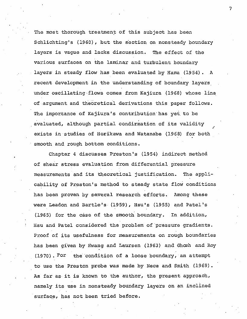
The most thorough treatment of this subject has been Schlichting's (1960), but the section on nonsteady boundary layers is vague and lacks discussion. The effect of the various surfaces on the laminar and turbulent boundary layers in steady flow has been evaluated by Hama (19 54) . A recent development in the understanding of boundary layers under oscillating flows comes from Kajiura (1968) whose line of argument and theoretical derivations this paper follows. The importance of Kajiura's contribution'has yet. to be evaluated, although partial condirmation of its validity exists in studies of Horikawa and Watanabe (1968) for both smooth and rough bottom conditions.

Chapter 4 discusses Preston's (19 54) indirect method of shear stress evaluation from differential pressure measurements and its theoretical justification. The appli­cability of Preston's method to steady state flow conditions has been proven by several research efforts. Among these were Leadon and Bartle's (1959), Hsu's (1955) and Patel's (1965) for the case of the smooth boundary. In addition,Hsu and Patel considered the problem of pressure gradients. Proof of its usefulness for measurements on rough boundaries has been given by Hwang and Laursen (1963) and Ghosh and Roy (1970). For the condition of a loose boundary, an attempt to use the Preston probe was made by Nece and Smith (1969) . As far as it is known to the author, the present approach, namely its use in nonsteady boundary layers on an inclined surface, has not been tried before.

The argument, whether indirect methods of evaluation of the shear stress from pressure measurements, velocity profiles (Jonsson, 1963), or heat loss (Bradshaw, 1963) and aenomometry are essentially less correct than direct methods using shear plates (Eagleson, 1962; Iwagaki et. al., 1965, 1967; Yokosi and Kadoya, 1965; Petryk and Shen, 1969) has not been decided in favor of either side. Both contain inherent instrument-bred experimental problems. The resolu­tion of this question will probably have to be made by standardising procedures and objectives for both techniques.

The experimental, setup including instrumentation and / . techniques is described in Chapter 5. This study was carried out in a 3 x. 3 x 65-foot wave tank illustrated in Figure 6. Uniform wave forms and wave trains were generated with a paddle type wave machine, and allowed to run up on a fixed slope "beach" situated at the downstream end of the tank.Wave and velocity data were collected using resistance wave gauges and differential pressure probes, respectively, and their interrelation evaluated in presence of smooth and rough bottom boundary conditions. These instruments as well as the wave tank, were built by the author in 1967-68. Mass trans­port for various wave periods and amplitudes" was evaluated with the aid of high speed photography of neutrally buoyant particles.

Problems encountered in the design and operation of the facility are. described and recommendations in regard to future research are made in this chapter.

9

Experimental conditions and step-by-step experimental procedures are.described in Chapter 6.

In Chapter 7, collected experimental data are evaluated in terms of pertinent theory and previous knowledge on this subject.

Discussion of the results and conclusions derived from this study are presented in Chapter 8.

/

CHAPTER 2FUNDAMENTALS OF SHALLOW WATER WAVE THEORY

The theory of oscillatory waves and their mathe­matical derivation can be credited to Stokes (1845) and Lamb (193 2). For water waves in shallow water no single theory applies. Basic considerations rise from the classical solution of Stokes/ the first approximation of which is known as the Airy theory/ and its higher approxi­mations to the third order by Skjelbreia (1959) and to the fifth order by Skjelbreia and Hendrickson (1961) and De / (19 55). With d as the water depth and L the wavelength, for very shallow water the relative depth d/L < 1/25, and the surface configuration and internal velocity field be­comes so distorted that the use of sinusoidal theory be­comes totally impracticable. In this region the theory of solitary waves is applied (Keulegan and Patterson, 19 40) and its limit the cnoidal theory (Masch and Wiegel, 1959,. Wiegel, 19 60). A definition of wave parameters is presented in Figure 1, and a.summary of the theories in terms of limiting ratios in Figure 2.

1. Airy or progressive waves

When wave amplitude is small we can ignore the second order terms in the Navier-Stokes equation for two-

dimensional steady flow (Equation 3.1 which is discussed

in Chapter 3) for the effect of viscosity will be negligi­ble and obtain the following periodic solution, known as the velocity potential

, ag cosh k (y + d)* “ a """"cosh kd cos (kx " at) (2*1)

where u = -‘3<J>/dx and v = -3<|>/'<)y, a = amplitude of the wave measured from mean surface elevation, i.e. 1/2 H, y is the vertical coordinate, g the gravitational constant and H is waveheight, and •

a = (gk tanh kd) .(2.2)

2iris the wave angular frequency, so that a = ip— , where Tis .the wave period. This is related to the wave numberk = 2tt/L, and L is the wavelength.

When'.the depth is greater than 0.25 La 2 = gk = <3 (2.3)

and when the 'depth is very small in comparison to wave length'

£ = (gd) = C , (2.4)

where C is the wave phase velocity. Expanding we get

a qT . 2t t& ,gL , , 2iTd-4 ' C = k = 27 tanh ~ = (27 tanh (2’5)

In deep water d/L > 0.5, and the value of the hyperbolic

tangent approaches unity/ therefore for periodic wavesgL J*

C = ( -2.) (2.6)O 2ir

L0 = C.T (2.7)

CQ = gT/2n (2.8)

where the subscript refers to deep water conditions.In shallow water the value of (tanh 27rd/L) -»• 2Trd/L,

consequently the wave celerity becomes

C = (gd)h (2.9)Some useful functions are expressed by the ratiosL = (gT2/2it) tanh 2i,a/L = tanfa 2*d (2-10)L0 gTz/2ir L

which is the ratio of wave length in water of any depth to the length in deep water, allowing prognostication of wave celerity and energy conditions at a beach. Also

C (gT/2u) tanh 2ird/L , /T ii\c = g T / 2 -Tr--------- = t a n h 2,Ta/L t 2 -1:L)

which is. the effective decrease in wave velocity shoreward. Also

H ^ \ (2 12)iro <25c > 1 '

the wave steepness, where n is the coefficient of shoaling, Hq and H are the deep and shallow water wave heights

13

respectively; and finally

d d 2irdLq = l tanh - f - (2.13)

allows the calculation of relative, depth normal to the shore from information obtained on deep water waves.

Orbital motion of water particles can be described in the x-direction as a function of the velocity potential

u = M = agfc 9S£* <£*> o o s O c x - a t ) ( 2 .1 4 )

= ° g | s h 2 2 ^ ) / L « » • 2 * <E - I ' » . 1 5 )

where u is the horizontal component of orbital velocity distribution. Similarly, in the y-direction

. . ’ - g - Sc > inh <kx - <2 -“ >

H sinh 2rr(y+d)/L .x t.“ T sinh 2ird/L sin 2ir (2.17)

and v is the vertical component of orbital velocity.

Now in deep water d / L >1/2, and the radius of orbital particle motion is

r = e2”y/L° (2.IS)

and the terms cosl? 2lI.ft+d,>/L % slnk Sb e2’Iy/Le .sinh 2ird/L sinh 2ird/L

/

We can use this in

= umax = - I T e2y/Lo (2.19)itHq

Vmax

which shows that there is an exponential attenuation of waves with depth and steeper waves have a faster rate of attenuation as f(e) lies closer to the vertical axis.

In shallow water as the sinusoidal wave profile undergoes modification, the expressions for the wave characteristics are also modified.' The wave celerity in shallow water becomes

C = (2ii tanh 2-na/L)% (2.20)2 tt

'the length

L = 22. tanh 2ird/L . (2.21)Z IT

In shallow water the shape of water particle orbits becomes flattened as the bottom increasingly interferes with the wave, resulting in the increasingly longitudinal distortion of particle motion. The expression for the' orbital radius in the horizontal plane

H cosh 2tt (y+d) /L ,nrx = . 2 ' sinh 2ttd/H ~ (2*22)

and correspondingly

H sinh 2tt (y+d) /L .ry “ 2 sinh 2ud/L \z.Z3)

allows the calculation of the horizontal and vertical water particle velocities, which are

In summary it can be said that calculation of most primary parameters of periodic waves are relatively straightforward even in shallow water. For practical purposes these linear equations- are not only useful/ but widely employed.

2. Stokes wavesStokes (18 80) has shown, by application of con­

secutively higher order approximations of. sinusoidal wave theory, that there is mass transport in the direction of wave propagation. This means, that as water particles are moved back and forth in waves of finite amplitude, each particle moves further forward than it moves back, thus an increment of translation takes place with each passing wave. Stokes waves have small finite amplitude and wave steepness. The riiethod of approximation is to expand the velocity potential, <)>, about the still water level until a non-linear surface condition is reached, consisting of

- 13. cosh 2 ir (y+d)/L u “ T sinh 27rd/L (2.24)

and

_ ttH_ sinh 2ir(y+d)/L T sinh 2TTd/L (2.25)

an infinite series containing partial derivatives of the potential. To obtain solutions one must make successive approximations. Stokes waves lend themselves well to wave profile determinations in deep water but as De (1955) has shown, using fifth order theory, Stokes waves should not be used for d/L '< 0.125.

The deep water wave celerity for Stokes waves is

C = tanh 2Trd/L) ** . (2.26)

which is the same as in linear theory. To give a sampling / of consecutively higher approximations of various functions, the wave potential with respect to velocity is

* ■ § - t/T) +

The horizontal water particle velocity is given by

9 (j> ttH cosh 2it (y+d)/L ,x t.u - 9x “ T sinh 2Trd/L cos 27r(L_ T) +

I IS. iH cosh 4ff(y+d)/L 4u(x _ t . .4 T L sinh4 2Trd/L cos 4 1 l t'-.

The theory overestimates the vertical component while underestimating the horizontal velocity. The second term shows that there is a nonperiodic drift in the •

direction of wave advance which we call mass transport. Stokes calculated its velocity to be

— __ 1 jrH 7tH_ cosh 4Tr(y+d)/L U = o m t • • o ^2 T L sinh2 2ird/L (2.29)

The third approximation of wave celerity is of the form

C 2 = g tanh 2 ud [i+ (|H) (8 + cosh 87rd/L 8 sinh4 2frd/L

Further approximations ultimately converge in the form of a power series. The use of Stokes wave theory is most advantageous where waves are relatively steep as in'the case of wind effect superposition.

3. Solitary waves

Establishing and defining solitary wave properties is. attributable largely to Munk (1949) from the theory of unsteady flows of Boussinesq (1872). Munk found con­vergence to be slow for Stokes waves if d/L <<1/10, called these waves solitary and their limit as cnoidal waves. In a solitary wave the mass, transport occurs under the crest, but not under the trough. The wave velocity is

and the associated horizontal and vertical water particle

C = (gd)h [1 + §£] (2.31)

velocities are found to be, respectively

18

u = (gd) h sech2 [(3/4 H/d3)5 (x - Ct) ] (2.32)h y h

v = C3gd(d) 3)^ “ sech2 [ (3/4;j) (x - Ct)] •

tanh [(3/4|)^ (x - Ct)] (2.33)

Wave deformation is strong caused by the differential transport of water under the crest, being faster near the surface. Because 90 percent of the mass of water translated forward above the still water level is confined within limits of four times the depth we can calculate the volume of trans­lation or mass transport Q as /

Q = 4d2(§5)!s

Solitary wave theory is most closely descriptive of wave run-up even though it tends to overestimate it. It is applicable to waves in shoaling water just prior to breaking, the limiting case of which are treated as cnoidal waves.These limiting conditions were deduced by Laitone (1962) .

With the use of certain conventional limiting factors one can obtain an indication of which theory is applicable to a set of experimental conditions. The use of relative

, j

depth d/L, has been mentioned in this connection. Other parameters are H/T2 and d/T2. A more recent development is the so-called Ursell parameter H/L(^-)3 (Ursell, 1956), which Le Mehaute (1969) used to sort out the various linear and nonlinear theories. These relationships can be found in Figure 2.

CHAPTER 3 THE NATURE OF THE BOUNDARY LAYER

On of the characteristics of flow of any real fluid is that it has to work against resistance which has its origin in fluid viscosity. The mechanism, of resistance is the shear stress by which the slower moving layer of a fluid exerts a retarding force on the adjacent faster moving layer. The other characteristics of flow is that there can be no discontinuity between particles of fluid in motion, therefore no discontinuity of velocity. It has been observed that fluid actually in contact with a solid surface has no motion along that surface for molecules of fluid adhere to it. Consequently fluid velocity at the solid boundary is zero. Because successive layers move at increasing velocities in the direction away from the boundary, a transverse velocity gradient is created which approaches zero as the velocity reaches the free stream velocity at some elevation in the fluid. This gradient enables the solid surface to exert a drag force on the outer layers of flow. This region of the drag, explicit in the force of resistance, is known as the boundary layer - a limited thickness of fluid - adjacent to the surface. The force of resistance is tangential, i.e. par­allel with the solid wall. Because the shearing forces at the boundary are generated by viscous retardation, their resultant is called the viscous shear stress. It follows then, that the distribution of the shear stress normal to

20

the surface is a function of velocity. The descriptive parameters associated with it. and with the boundary layers hre the Reynolds number IR, the thickness of the boundary layers 6, and the local friction coefficient C f .

Prandtl's contribution (1904) to the theory of classi­cal hydrodynamics has been through observation of the dis­crepancy between his experimental results and that predicted by Euler's equation of motion. The theory had neglected fluid friction. Prandtl suggested that the flow about a solid object could be divided into two regions, a) a very / thin layer in the immediate vicinity of the body, where friction plays an essential part - the boundary layer -, and b) the remaining fluid region outside this layer where friction and thus the effect of viscosity, can be neglected. The mathematical treatment of this condition, i.e. incom­pressible flow with friction, is;carried out by using the Navier-Stokes equations of motion for a viscous fluid. For the case of unsteady flow under waves, two-dimensional case:

+ u|H+-v£i = -i ; vil* • (3.1) •31 3x 3y p 3x Y

where the condition of continuity of flow is met by

iE + = 0 (3.2)3x ' 3y

and where the x-axis is positiveoin the direction of wave propagation, y is the vertical coordinate, positive upward;

21

is the kinematic viscosity, the density of fluid, u and v the local velocity terms in the horizontal and vertical directions respectively and p is pressure.

The boundary conditions at the bottom and the surface, respectively, are

y = 0, u = 0, v = 0 and y = 00, u = U (x, t)

where U(x,t)' is the free stream velocity. Neglecting con­vective terms Eq. 3.1 becomes the nonsteady Bernoulli equation

_1 i£ = au + 0 9U’ (3 3)'p 3x at 3x

The free stream velocity has an oscillatory component, which can be written

U (x, t) = U(x) + Ui (x, t)U x (x,t)= U 1ei0t (3.4)

and the average of the second term vanishes, so that

U x(x,t) = 0 (3.5)Substituting Eq. 3.5 into Eq. 3.3 and averaging gives

r dU dU. 1 3p , .u - s + a i $ 1 = - j r a ? < 3 - 6 >

Following Schlichting'-s (1960) procedure, Eq. 3.1 then will yield

1 Hi= iEi+ v iiSi (3 7 )31 31 3y2

22

after the non-linear convection terms have been omitted, on the condition that they are negligible if 5 « L, whereis the boundary layer thickness and L is the wave length. Dropping the subscript 1 , as we deal only with the periodic component, Eq. 3.7 can be rearranged into

and Eq. 3.6 into

iLLI = 2 E (3 q\3t p 3x

where (3.8) is the equation for oscillatory motion in the / boundary layer as used by Kajiura (1968), and otherwise known as the defect velocity relationship. In this notation z is the vertical coordinate taken from the bottom upward, t is the horizontal shear stress and U is the horizontal velocity just outside the boundary layer, derived from potential wave theory, so that

(3.8)

U = aC sin(kx - 3t) (3.10)

awhere a = ^ a dimensionless parameter, a is the wave amplitude2 7Td is the water depth, C is the wave celerity and k= — is the

wave number. Recalling that 6 « L we can assume

— = 0 for 0 < z < 6 3z

(3.11)

with boundary conditions of u = 0 for z = 0t 0 as z -»■ 6

According to Schlichting (1960) the validity of Eq. 3.7 can be established if the oscillating boundary layer thickness

,2v u5 = •(— >* (3.12)

where 6=2rc/T is the wave frequency number, is small compared to the steady-state boundary.layer thickness. Thickness, a length term, is the effect of the boundary layer on the flow outside.

1. The laminar case.When the frequency of oscillation is high a thin fric- /

,tional'layer will exist adjacent to the boundary, whose behavior is governed by viscous effects. Outside this layer the magnitude or nature of flow will be independent of vis­cosity. Stewartson (1960) has summarized theories pertaining • to unsteady laminar boundary layers. The special case of a fluctuating layer has been treated by Grosch (1962), who ascertained that an exact solution of the unsteady laminar boundary layer equations exists in the form of a power series in the phase kx-crt. If a « 1, or in any case for a in a sufficiently small region near kx-at=0, the linear theory provides an adequate description of the flow. The solution for the wave flow is analogous to the Blasius series for steady flows.

What is open to question, however, is whether the use of linear approximations for the boundary flow can be justi­fied for the case of a sloping bottom when the main part of

24

the flow behaves according to non-linear finite amplitude wave theory. The general equation for the horizontal velocity component, u, in the boundary layer, given by Iwagaki et al. (1965) in terms of the free stream velocity

u = U (x) [sin at - e“^z sin(at - 0zj ] (3.13)

is known-as the classical "shear wave" equation, where

0 = y/7/2v = s"1 (3.14)

/which is analogous to the solution derived by Grosch (1962) for the so-called linearized theory. Expressing Eq. 3.13 in cosine terms, we obtain the solution of Longuet-Higgins1 (1958) after application of Airy's small amplitude wave theory of Equation 3.7.

uQ = U [cos (at-kx) -e Z//(SL Cos (at-kx-z/SL) ] (3.15)

where the subscript "o" pertains to boundary conditions, and

U = sinh 1 kd (3.16)k •and 6l = (2v/a)'2 is the boundary layer thickness as shown m

Eq. 3.12. Subsequently, Eq. 3.15 will become simplified forat-kx=0, which stipulates conditions examined only under thewave crest and wave trough, so that

ug— = 1 - e " z/ 5L c o s (-z/<!>l ) (3.17)

For laminar flows, the bottom shear stress is a func­tion of the velocity gradient, and is usually expressed in the form

To “ z=0 (3.18)where u is the dynamic viscosity.

Denoting amplitude by M t can be expressed in terms of the boundary friction velocity u*

A

(U*) 2 • (3.19)/

Introducing Kajiura's (1968) modified friction velocity u*, Eq. 3.19 then becomes:

A

To— = u* u* (3.20)p o

Based on a solution given by Grosch (1962) for the shear stress term from linear theory, the approximate equation given by Iwagaki et al. (1967) is

= IR- '2 s in(kx-crt~j) (3 .21)puz 4

withIR = ------------------ (S£) (H) - 1 T&L. (3 .22)2sinh2kd v L 2ir v

In this expression IRis the wave Reynolds number. The con­vective terms, being negligible, have been omitted. It is interesting to note here, that the expression in the brackets contains tt/ 4 which is'the'maximum phase lag for the ratio

26

uQ/U and the shear stress in laminar boundary layers, theoretically also derived by Kajiura (1968) and experi- mentally confirmed by Horikawa and Watanabe (1968).

Iwagaki ejt al. (1965) obtained the equation for the maximum shear stress by use of Eq. 3.12 as

Tomax = /2v ,tn j npgh ' g sinh kd V

Now entering Eq. 3.16, we get,2vtt ^

Tomax ~ T (3.24)/

which expresses the fact that the maximum boundary shear 'stress is a function of the outside velocity and the bound­ary layer thickness only.

Rearranging terms in Eq. 3.22 and substituting Eq. 3.16, we get

IR_i£ = ^ ' (3.25)

IR% = (3.26)vI i < -/■where 6L = (v/a) =6^//2 for smooth bottom. This expression

is similar to that of Kajiura (1968) and Horikawa- and Watanabe (1968).

Eagleson's (1962) definition of the average bottom friction coefficient, defined by

cf = (3*27)

has been modified by Iwagaki et al^ (1967) and for linear­ized theory expressed as

C, = 8 (-£---) % = 6.39 3R (3.28)X IT ]R

2. The Turbulent CaseThe general expression for the velocity distribution

in a turbulent boundary layer in its simplest form was suggested by Prandtl:

£ = (f)n (3.29)/

where n is approximately 1/7 for moderate Reynolds numbers.Consequently the shear stress distribution does not followthe form of :3'.u/3z anymore, and while Eq. 3.29 satisfactorilydescribes the velocity distribution in most of the layer, at

_JL _ 6 .the boundary itself 3u/3z = 1/7 U3 7 y 7 = « for z=0, which which expression is nonsensical. However, sandwiched between the turbulent boundary layer and the solid surface is the laminar sublayer, whose velocity profile is taken to be linear, corresponding to the laminar boundary layer structure.

Particular solutions for the velocity distribution in a turbulent boundary layer have been attempted in terms of a single parameter, (Dryden 1948), such as the momentum thick- ness

/oo u uQ (1 - u) (u) <*z (3.30)

and the displacement thickness

28

(3.31)

The distribution is nevertheless governed by the shear stress at the wall and the pressure gradient. The most commonly

which is related to the shape of the flow field. The valid­ity of the hypothesis is often questioned, because the shear stress apparently is more closely related to turbulent pressure than to the local mean velocity gradient in a great number o f 'cases.

Nevertheless, in view of the lack of a workable alter-/ native, the mixing length hypothesis, and thus the related "law of the wall" principle, has been employed in this thesis. Justification for its use is made in Chapter.4 as well as in the following paragraphs.

For the laminar sublayer of a turbulent boundary layer, across its width, the shearing stress is constant. The generalized velocity equation of the sublayer for a smooth

is linear in form. The correlation between the terms u/u* and zu*/v can be extended far into the turbulent field (Clauser, 1956), which is also corelatable by the defect

eimployed theory applies Prandtl's mixing length hypothesis,

flooru u* (3.32)u* z—V

velocity term (u - U)/u* and z/S. Figure 3 exemplifies the overlapping of the two methods of correlation..

29

The general form of the equation of turbulent flow

u = A log'(zu*/v) + C ■ (3.33)or

u-U = A log(z/v) + B (3.34)

must be appraised experimentally for any one case in terms of the constants A, B and C.

Eq. 3.34 in presence of a rough boundary must take into account the roughness elements. This expression modifies to

- = A log — + C - — •* (3.35)u* v u*where Au/u* represents the vertical shift of the logarithmic profile caused by roughness. This shift is a function of the local Reynolds number,, and can only be determined experi­mentally. For large values of 3R the laminar sublayer dis­appears, and the influence of viscosity declines drastically. The general expression, for the outer, turbulent portion must take into account then the presence or absence of the laminar sublayer, so that

= A log + B - C - (3.3.6)u* • v u*

The universal shear distribution for turbulent boundary layers is given by Clauser (1956) as

=. “f\ (f>- (3-37)

30

where £' is the derivative of the Lagrangian stream function V .It follows then that

T = Kz (f|) (3.38)

because the scale of turbulence and the thickness of the boundary layer are governed by the scale of the eddies as a function of distance from the wall. Kz is the Boussinesq effective viscosity or Kajiura's (1968) vertical eddy viscosity. The difficulty remains, however, in defining <S, the boundary layer thickness, which is a function of time. Unless velocity profiles in the boundary layer can be experi­mentally established, none of the theoretical approximations, such as that of Eagleson (1959), who used the Karman-Pohlhausen method, will satisfy the.equation of motion. Consequently the distribution of turbulent shear stress cannot be related to any definite scientific principle (Yalin and Russell, 19 66).

Turning now to unsteady boundary layers under waves, the difficulty outlined previously, i.e. finding exact solutions, becomes amplified for time-periodic equations which are non­linear in character. This problem can be eased by dealing with only instantaneous values, rather than involving the entire "history" of the flow, related to the stochastic nature of turbulence. Specifically, maxima of such param­eters as velocity, boundary layer thickness and shear velocity can be investigated. The use of steady state analogy can be justified for oscillatory flows when such

postulates are met. As in the case of drag coefficient, under oscillatory flow it is time-variant, but when the shear stress is near its maximum value, the drag coefficient is found very nearly the same as in steady open channel flow of the same boundary conditions (Jonsson, 1965).

The existence of a universal velocity distribution in an oscillatory turbulent boundary layer was confirmed by Jonsson (1966) in terms of the "law of the wall" and the "defect law". The breakdown of velocity distributions in the inner and outer layers of flow is similar to that /

studied by Clauser (1960) and Mellor and Gibson (1966). and theoretically analyzed in presence of pressure gradients by Mellor (1966).

■ The structure of the turbulent boundary layer is shown in Figure '4 which demonstrates that conditions in the overlap layer can be described by both the logarithmic and the defect layer equations. Clauser's (1954) discovery, that the defect portion is an equilibrium boundary layer is exclusively de­termined by the pressure gradient parameter 6 * (dp/dx)/ t q ,

has been further refined by Mellor and Gibson (1966) who stated that the defect profiles can be matched with the logarithmic portion of .the law of the wall for small values of z and small values of Clauser's parameter. This allows the determination of the skin friction coefficient.

The general equation for all subdivisions of the boundary layer is given by Kajiura'(1968) as:

.32u*/9z2 “ (icr/K2)u* = 0 . (3.39)

Using the general equation for the vertical eddy vis­cosity (Eq. 3.38), Kajiura (1968) introduced conditional values of K_ based on the tripartite division of the tur- bulent boundary layer for the case of smooth bottom.

Kz =

v for 0 <_ z < Dl in the inner layerKu*z for DL < z < d in the overlap layer (3.40)Kj for d <. z < 6 in the outer layer

where DL = Nv/ft* is the thickness of the viscous sublayer, /and N = 12 is assumed, d is the upper limit of the overlaplayer, < = 0.4 is Karman's universal constant, and I<d =icu*d= KU J , where K is a universal constant with a value o Lof 0.2 and 5' is the wave displacement thickness. The re- Lliability of K is questionable and yet must be confirmed experimentally (Kajiura, 19 70,.personal communication).

The velocity profile for the case of the smooth bottom, has the general form

<S2u* • ,a— rr- - i (—) u* = 0 . for the inner layerV6 z‘

32U*' 3Z 2 ~ 'KU* Z- i (^-%r— )u* = 0 for the overlap layer (3.41)

32u * i (£_) u* = 0 for the outer layer3 z2 ' Kd '

Integration of the above quantities gives

33

u*— = A sinh. 3L CDL*-z)+cosh. 3,L (PL-z) for the inner UL layer

U u* (sinh 3rDr+ A cosh 3tDt ) for the overlap (3.42)L L layer

U-uu* "o' '"cTd= u*/(K,3_) e"^d(z"d) for the outer layer

where u*, u* are the shear velocity at d and D respectively, d L L

„ ,o,^ iir/4 /3l ,= (-) e '■ (3.43).

andi

/ a. iTr/4 • , a. . ir , . . it. . ..3d = e “ Kd 4 lsin'4’ (3.44)

includes the phase lag in the boundary layer.

Writing the bottom shear stress, in terms of the frictioncoefficient, we obtain. i

C£JU = 1° (3.45)

C f '=T0/ p U 2 (3.46)

wh;ich for small values of IR and U/azQ reduces to C f = 1/IR .

For shallow water Kajiura gives

t0 = H Amp (dp/dx) (3.47)

Cf = £| (3.48)U

34

where the amplitude of Cf and its phase 0 can be expressed in terms of IR=U6^/v for the smooth bottom. Interestingly, the value of 0 increases up to ir/ 2 for shallow water.

For the case of the rough boundary, the difference from the smooth bottom is in the eddy viscosity assumption, where

yicu* Dr for 0 <. z < DR in the inner layer

ku£ z for Dr < z ± d in the overlap layer (3.49)K z =

k u* d for d < z in the outer layer/

with y = (lnlS) ” 1 =.369 and D = 15z specifying the heightR O. ■of the inner layer in which the eddy viscosity.is constant,zq is the characteristic roughness length. Experiments ofHorikawa and Watanabe (1968) indicate considerable timevariation in K for z < DT and z <. and some degree of z L Rattenuation as'well near z=0'. The period of this time variation is %T and also a function of z .

The friction coefficient for rough bottom given by Kajiura is

C f = ( ! £ l ! ° ) 2 (3.50)UyRK

where yR is the upper" limit of the inner layer, and the Reynolds number derived is

U , ’ ' '60' 4\ i5i)

35

indicating that the amplitude and phase of the friction coefficient increases with decreasing values of IR . For

A 'small values of IR and U/0 zo ,

Cf = 1.70(U/oz0) (3.52)

Employing Kajiura's classifications we can now define the hydraulic flow regimes in terms of the Reynolds numbers. The transitional region for smooth bottom., using Eq. 3.26 is expressed by

25 < IR < 650 (L = smooth bottom) (3.53)/Xj

and for rough bottom, using

m = UD ‘ (3.54)v

100 < IR_ < 1000 (R = rough bottom) (3.55)X\

where D = 30zQ is Nikuradse's equivalent roughness, and zQ is the roughness length, i.e. the representative grain size on the bed.

' In a*’report by Jonsson (1965) the transitional range 500<UD/v<1000 is further characterized by the boundary Reynolds number, IR 5= Umax6/v. Jonsson. states that smooth turbulence begins at IRg = 250 on a smooth floor. Collins (1963) reports this critical Reynolds number to have the value of 160, using the orbital velocity at the bed in the expression, which in terms of IRL is equivalent to a value of 113.

3. The effect of the pressure gradientsThe previous discussion on the use of the Navier-Stokes

equations for.the two-dimensional case assumed the knowledge of the local pressure distribution. The approximate solutions obtained by various investigators were for the condition of zero pressure gradient. The problem of correct mathematical descriptions becomes amplified in the presence of adverse (positive) or favorable (negative) pressure gradients as th’e position of separation is approached. Solutions, based on the "similarity" principle can be obtained if the velocity distribution in the free stream is proportional, e.g., to ex . The criterion of correction solution is in the observa­tion that uQ <• U. Clearly, this is not the case when the maximum mass transport takes place in the vicinity of the boundary.

Because the boundary layer fluctuates in thickness and the sign of u reverses periodically passing through zero, the interaction between u and v (the local hori­zontal and vertical velocity components respectively) becomes important. Experiments by Dryden (1948) show, that in the case of turbulent flow in the boundary layer, the decrease in shear stress is correlatable to the decrease . ' of interaction between u and v, although the magnitude of local fluctuation u 1, v', remains stable as separation is approached. Longuet-Higgins (1958) attributes boundary layer growth and dissipation in part to the effect of

vertical velocity components, and proves that the inter­action term is negative in sign, which in turn gives rise to the phenomenon of mass transport.

Mellor (1966) in discussing the effects of zero and positive pressure gradients established that the true • shear stress r, is a function of the local pressure gradi­ents , so that

(U*) 2 = (Ujj 2 + i (3*56)

T = T i:- i£ . (3. 5iyo dxi.e. in the viscous sublayer. Let us recall that for small values of Clauser's parameter

(6* 1E)/t0 (3.58)3x .

in equilibrium boundary layers the velocity profiles of the defect layer is logarithmic and can be matched'with the logarithmic profile of the wall layer. Mellor (19 6 6 ) con­cluded that in contrast to this case, if the value of this parameter is large, the main stream velocity distribution has the form

U . c X2 x Mn _Q.U “ -1' " 6* ) (3.59)owhere and &* are initial values of U and 6*. Now o o.m-Const.=-.230 and the flow is completely determined by

38

In other words, the flow is influenced by the pressure gradient if the value of is small. Then examining the boundary layer as separation is approached, one can note that the value of shear stress decreases before changing signs, as the pressure term plays an increasingly important role. Furthermore the flow is not in "equilibrium" and the wall layer and defect.layer profiles do• not match anymore.Mellor*s results were later extended to include the case of favorable pressure gradients by Herring and Norbury (1967)•

One'also does not know what the true value of the bottom shear stress is under these conditions. Mellor (1966) indi^ . cated that the actual value of t or t q lags the valu.e, which would have been obtained, had the flow been in equilibrium, i.e. X- constant. In examining Eq. 3.51, we will note that this can only be met if dp/dx is near zero. This condition exists only under the wave crest and the wave trough, however. Consequently, any evaluation of local shear stress conditions is limited to these intercepts'of the wave cycle by the re­quirement of boundary layer equilibrium, which is character­ized by a known continuous function of the velocity profile, a measure of true shear and a boundary layer whose growth has attained, or is approaching the maximum. Furthermore, the local value of v‘ is zero and t q is at maximum.

CHAPTER 4EVALUATION OF SHEAR STRESS FROM PRESSURE MEASUREMENTS

The various direct and indirect methods employed in the measurement of skin friction have been outlined in Chapter 1. The present chapter is primarily concerned with theoretical development behind the indirect measurement of shear stress by use of a surface Pitot tube.

In the original paper on this subject, Preston (1954) advanced the theory that because there exists a region close to a solid surface in which 'the conditions are only

✓. functions of skin friction, local fluid parameters and a "suitable length", there should be a universal non- dimensional relationship between the total pressure as recorded by the stagnation tube, in the flow and the static pressure at the wall. Furthermore, he advanced the idea that this relation is independent of the pressure gradientin the turbulent boundary lay- ir.

(

In re-examining Eq. 3.37, we find that the velocity distribution in the turbulent boundary layer, based on the "inner law" (or law of the wall) principle has the form

where y is the distance from the boundary, and u* = (t / p )^

is the shear velocity. This functional relationship reduces to U/u* = yu*/v in the laminar sublayer (Eq. 3.30), where flow conditions are predominantly governed by the kinetic

viscosity. In numerical terms, Eq. 4.1 can be expressed as

The 1/7 power law has been mentioned in Chapter 3, and will be made further use of in Preston's equations. .

Instead of measuring the velocity at a point close to the wall, from dimensional analysis we may consider the

Pitot tube" and the static pressure recorded either by a. static tube.:or tap. The pressure difference between the two probes can be expressed in functional form.

where f2/ £ 3 are unknown functions, d is the outside diam­eter of the Pitot tube, tq the boundary, shear stress, Ap=P-pQ is the dynamic pressure recorded by the surface Pitot tube (hereafter referred to as the Preston tube), pQ is the static pressure recorded by other means, and p^v are the density

, j

and kinematic viscosity of the fluid, respectively.

The above relationship was originally established by Preston (1954) and experimentally verified for turbulent boundary layers in pipe flow with zero pressure gradients.The numerical relationship obtained by Preston, for the

= 8.67 (Zlii) l/7Uw v (4.2)

difference between the total pressure recorded by a surface

(4.3)or

(4.4)

fully turbulent region of the flow assumed a logarithmic* ’ * *•

relationship of

lQ9lO = 2 ' « 04 + JlP«10 (4'5)for the range of 4.5 < log^Q (Apd2/4pv2) < 6.5/ and this is shown in Figure 4.

In plotting his calibration curve, Preston became rather concerned with what he termed the "displacement of the effec­tive center" e,‘ an incremental error in reading attributed tothe change in flow pattern restricted by a circular probe in •

/ •contact with the solid surface. Referring to the work of Young and Maas. (1936) he came to the conclusion that e/d varied between 0.12 and 0.18. Implementation of this param­eter was carried out by Patel (1965) who verified Preston's assumptions for the shear-pressure relationship in presence of adverse and favorable pressure gradients, and agreed with Preston on the existence of an effective center displacement. Using theoretical work of McMillan (1956), Patel noted that the effective velocity Up as recorded by the Preston tube, using the relation

is the true velocity at y = 1 / 2 Kd, where

K = K(H,*,—) only, is undefined. (4.7)v t

From these considerations Patel derived a Preston-tube

42

calibration curve in three parts, corresponding to the inner, overlap a.nd outer layers of flow. These equations contain corrective terms for e in forms of constants A,B, C prescribed by McMillan (1956), whose values are un­determined for oscillating flow. Consequently, we followed Preston's original development as well as refinements brought out by Hsu (1955). ,

Hsu's contribution consisted of making measurements in both zero and mild adverse pressure gradients. For the laminar sublayer (or inner layer) he modified Eq. 4.5 to

✓read .•

1Og10 j f £ ■ 1/2 ^ 1 0 (4 ^ > + 1/2 1O*10 ' (4-8>

which is nearly identical with Preston's expression for viscous flow

T0 d2 Apd2log10 4pv2 = 1//2 log10. 2 + loglQ 4pv2 (4.9)

assuming no displacement of the effective center.

The parameter t = a/d in Eq. 4.8 is the ratio of the inner to outer diameter of the probe. Preston utilized proves with a wide range of t, and found the value of 0 . 6

to give most consistent calibration results.For the turbulent portion of the boundary layer Hsu

gave the expression

tQd 2 71O910 = 1 °S1 0 k + 8

Apd2logio W (4.10)

where k = I (t) , and the function X(t) has been evaluated and tabulated by Hsu. The consideration given the propor­tions of the probe has little effect of the basic expression, Eg. 4.5, for values of t in the neighborhood of 0.6. This is evident from Figure 5,- showing that the two relationships plotted nearly overlap.

The velocity distribution in a laminar boundary layer is similar to that of the inner layer. The expressions for each are identical (Eq. 3.30). Therefore, it is justified to use Eg. 4.8 in measuring the dynamic pressure distribution' m a laminar boundary layer and obtaining values, of shear stress from it.

The effect of boundary roughness on the Preston tube and essentially the validity of the method has been examined by Hwang and Laursen (1963) and more recently by Ghosh and Roy (1970). By expansion of the expression

Ar = i f ;u >2 C4.il)t 0 '• 2 u b 2 -J5. d £

where £ = -jta&/2 and a is the inner diameter, Hwang andi

Laursen obtained a convergent series which takes the boundary roughness into consideration but is based on the Karman- Prandtl velocity distribution for open channels. Although Hwang and Laursen confirmed the applicability of the Preston method for rough surfaces, Granville (1963) took issue with their procedure of single point measurement and recommended a survey of the velocity distribution.

44

Ghosh, and Roy (197Q) refined Eq. 4.11; their experi­ments in part having been similar in scope to Hwang's and Laursen's. Confirmation given by them for Preston method is on the basis of least dispersion of experimental data.

Clearly neither of these semi-empirical formulae can be used here, even though the inclusion of the effect of size of roughness' makes them attractive, because of the dissimilarity of main flow conditions - steady-state vs. harmonic motion. Thus we are left with either Preston's expression (Eq. 4.5) or Hsu's (Eq. 4.10) for turbulent flow conditions. The use of neither can be fully justified until experiments can be carried out simultaneously in steady- and unsteady-state flow using identical test conditions.

For this paper Eq. 4.10 was chosen because it incor­porates the probe dimensions. It shall be shown in Chapter •5 that only a small portion of the experimental data could be fitted to this equation.

The effect of pressure gradients on the Preston tube. should also.be mentioned. Although Hsu (1955) confirmed the applicability of this technique for mild adverse pres­sure gradients, later results of Patel (1965) indicate that 'for severe favourable’ and adverse pressure gradients the Preston tube overestimates skin friction. Based on this fact, as on other considerations discussed in Chapter 3, the condition of zero pressure gradient, which exists under the wave crest and trough was chosen in the experiments.

There is considerable disagreement in the literature concerning the nature of the hydrostatic pressure distribu­tion under waves transforming on a slope. We know that in the Airy theory the hydrostatic pressure head is zero. Ursell

. (1953) noted that.this assumption also holds for the second- order Stokes theory. Investigations of Dorrestein (1961) indicate, however, that vertical accelerations in the moving fluid change the effective water density, the effect of which does not vanish in the average. Consequently, for linear shallow-water approximations on a sloping beach

/

p - ps « pg(rT - z) - pU2 .• (4.12)

where p is the pressure and u 2 the mean square velocity at some point in the fluid, pg = pressure at the surface, Yi = the vertical displacement of water surface from mean eleva­tion, and z = the vertical coordinate. The above equation differs from the standard hydrostatic expression by the term -PU2, which is related to the mean water level correctionU 2/g. That is to say: due to wave setup on beaches thehydrostatic pressure will have an x-wise component even though the instantaneous slope of the surface is zero. According to Ippen (1966) the hydrostatic pressure distri­bution is less than predicted by pg.An under the wave crest and greater under the trough. The gradient is neverthelessdepicted as having a linear trend. In a theoretical analysisof the limiting conditions for cnoidal and Stokes waves,

Laitone (1962) states that the pressure gradient becomes non-hydrostatic only near the wave crest.

In a summary on wave theories, LeMehaute (1969) states that in the case of linearized theories (small amplitude, first-order cnoidal) the pressure distribution may be assumed hydrostatic. For non-linear treatment of waves, the effect of.the convective terms in the Navier-Stokes and Bernoulli equations cannot be neglected and on approaching the solitary wave state the pressure is no longer hydrostatic.

In view of the above inconsistencies and because wave/ data has been analyzed by use of linearized theories in these experiments, the above problem was decided in favor of a hydrostatic pressure distribution for (kx--at) = 0 .

CHAPTER 5EXPERIMENTAL APPARATUS

1. The wave tankA fixed level open channel, with concrete-and plexiglas

walls and dimensions of 65 x 3 x 3 feet was constructed in 1968-69 in the Hydraulic Laboratory of the Department of Civil Engineering (Figures 6 , 7) . Part of the structure had existed in'the form of a 40-foot long open-end flume with concrete walls and floor, as well as two opposing glass window inserts, 8x3 feet x 1/2 inch in dimension. In de- signing the addition, the major consideration was to obtain the longest possible extent within the structural limita­tions of the indoor laboratory, in order to ensure that two- dimensional studies could be conducted in the facility. Consequently, the arbitrary length of 65 feet was obtained. Other considerations included access to the tank and visi­bility of the operating processes in the experimental portion. The latter was accomplished by adding two 20-foot long plexi­glas wall sections opposing one another in the downstream section of the channel. One-inch thick Lucite sheets in four sections were secured to aluminum frames built from angles and milled I-beams. The first time the tank was put into operation, the plexiglas section buckled outward due to the stress of the water in the tank, subsequently both walls had to be reinforced with eight inch wide channel steel along the length of each wall. The downstream end was closed with a

1 / 2 inch thick aluminum plate which remains removable forpurposes of trucking in sand or instruments. Both the endplate and the custom fitted, milled plexiglas panes weresealed with Dow-Corning No. 780 Silicone caulking compoundwhere in contact with porous cement surfaces. Adjacent tometal surfaces Dow-Corning No. 781 sealer was used. Allcontact surfaces were gasketed before application of thecaulk. In the preparation of the panes, sufficient clearancewas left for expansion between window sections. The thermalcoefficient of plexiglas is 5x10 in./in/°F., A mean tempera-

/ture of 72°F was assumed, with extremes on the order of ±15°F

Both channel-irons securing the wall-tops were leveled three dimensionally prior to installation of a track and instrument carriage to run the length of the facility. The track consists of two sections of elevated U-strut, 60 feet long on each side, supported by 28 machined, tapped aluminum angles shown in detail on Figure 6 . Four aluminum blocks with pins were attached in the open ends of the U-struts in order to hold two stretched roller chains in place.

A 36x15^ inch welded aluminum frame outfitted with ad­justable axles and wheels serves as ah instrument carriage. Power to it is supplied by a forward-reverse gear, variable speed, 1/8 HP electric motor, which drives a 1/2 inch shaft through, a chain type transmission. Traction is provided by sprockets in the chain at each end of the driveshaft. The open frame allows nearly unrestricted positioning of the

various instruments placed into the flow field.The water input and drainage system, while adequate for

this study, is not efficient and will have to be modified. ,The original structure contained an eight-inch input pipewith valve at the■upstrearn end of the tank, connected to asump. However, in practice the tank was filled with tapwater through an overhead three-inch pipe. Drainage isprovided by a four-inch valved pipe at the midsection of thechannel. Because the tank was subsequently partitioned inits downstream portion with a fixed slope "beach", only the

/water under the beach could be drained directly through this outlet, the remainder and larger quantity of fluid above the "beach" had to be siphoned out. It was necessary to fill the cavity under the partition with water to maintain equal pres­sure on the "beach".

Difficulties were encountered in prolonged use of the water contained.in the tank, as the plate tended to corrode rapidly. Tests showed the pH of water to change from 6.9 to 8 . 8 within 3 days after filling the tank, and in contra­diction to this basic condition, precipitates of oxides accumulated on the plate, roughening the surface and requir­ing frequent cleaning and scraping. Figure 8 illustrates the various free aluminum ions available in a similar system. It is surmised that the nature of the precipitate is A1(OH)4 . Since the chemical composition of the compound could not be ascertained, the solution to the problem was found in weekly draining, cleaning and refilling of the wave tank.

To study wave transformation, a fixed 1:12.5 slope "beach" was constructed of wood 2x4*s and marine plywood at the downstream end of the channel. Because a smooth J surface was desired for initial experiments, a 1/ 8 " thick aluminum plate in .two sections was secured to the plywood face along its 25-foot length. The entire "beach" in contact with walls and floor was gasketed and sealed with commercial air-conditioning duct tape which prevents circulation across the plate.

The use of a metal plate, while enhancing chances of/electrolysis, made it relatively easy to attach various

roughnesses to the slope, not only ensuring an even surface, but also enabling a least problematic removal of the sand. The use of the Preston probe, described in Section 5 of this chapter, is not feasible in presence of movable bedload. Therefore, sand with median grain diameter of 0.36. mm. was glued to the "beach" surface using Dow-Corning Sealer No. 780, in one-grain diameter thickness. Experiments conducted on this surface are referred to as rough boundary conditions as opposed to the smooth boundary of the aluminum plate. Ninety percent of the beach was visible through the ob­servation windows from both sides of the beach, facilitat­ing accurate placement of probes and gauges at desired elevations.

2. The wave generatorA belt-driven variable speed ratio wave machine,

attached to a paddle, was capable of generating waves of a wide range of frequencies and amplitudes (Figure 9).Driven by a 3/4 HP, 3-phase, 230V., 60C., 17-rpm full-rated- load electric motor, the Reeves-type mechanism could generate waves with 0.5<T<5.0 seconds depending on transmission gear ratio employed. Stroke variation of 2.62 inches to 13.5 inches was achieved by adjustment of the driving arm attached to a-flywheel, which produced wave amplitudes in the range of 0.05 to 0.205 feet. The paddle was hinged at the bottom of the tank and mQved at its top by a .fixed . arm and could be displaced from a minimum of 2 . 6 inches to a maximum of 9.5 inches in 2.0 feet of water depth. The slightly greater acceleration at the top of the paddle created whitecaps in.short period waves due to the asym-. metricity of the initial form. To remedy this, baffles were placed in frpnt and back of the paddle, as illustrated in Figures 6 and 9. Stiff wire cloth with %-inch opening .mesh was chosen for this purpose after some experimentation and consultation '(see Keulegan, 1969) and box-shaped baffles made from several layers of cloth. Further energy was absorbed by installing a sloping rubble mound, tied down with mesh, behind the wave maker and to some extent by the "beach" slope.

3. Wave gaugesIn model studies involving wave action, the procure­

ment of reliable results is predicated upon the development of an accurate wave-height measuring device. The governing factor in designing such an instrument is wave period. Considering that, Froude principles of dynamic (geometric) similitude show the relation tp = tm /A, where tp is the characteristic prototype time and t the same for the model,we define A as the scale ratio 1_/1_ (1^ and 1„ are repre-p m p m c .

sentative length scales in the prototype and model respec­tively) , and find that a wave period reduction on the order*^ of 1 0 -'1' for the model is common, somewhere in'the range of0.5-2.5 seconds. These short period waves require some electronic means of measurement, with high frequency response, especially in presence of higher order harmonics.

For this study the parallel-wire resistance-type wave gauge, similar to the one used by Dean and Ursell (1959), was adopted. Several other designs exist (Wiegel, 1956).The probe consists of two NiCr 1-mil diameter wires mounted side by side, stretched between two insulating plates. The wires are two inches' apart at the top place and 2 1 / 8 inches apart at the bottom to improve•linearity of response (Keuleganr 1969). The wires are charged from a 1200 cycle/ second oscillator of a Sanborn Model 150 carrier-preamplifier (Figure 10). When placed vertically into the tank and immersed to some depth, the wires of the wave meter act

53

as electrodes to complete an a.c. circuit. Any movement of the water surface causes a variation in resistance on one leg of a balanced Wheatstone-bridge circuit (Figure 11), which amplifies the output in the current proportionally to the change in water surface elevation.

Calibration of the instrument is carried out by sub­merging the gauge in still water at a desired elevation and balancing the open circuit. This is necessary because the two probes' of the instrument1 usually have slightly varying physical properties.. During incremental submergence, cor- responding'deflections are noted on the Sanborn oscillograph, the output' being in miliiamperes,. This type gauge is especially responsive to measuring small amplitude variations. The straight line relationship between submergence and current drain exists only about the balanced level of the electrodes owing in part to. the non-linear characteristics of the detecting, apparatus. Calibration curves, Figure 12, were drawn regularly for various combinations of the four wave gauges and four Wheatstone-bridges used, and it was found that for the same reference level the gauge output remained stable (within 3 percent). Several mechanical checks with point gauges as recommended by Wiegel (1956) confirmed the accuracy of these instruments when read in the linear portion of the.plotted calibration curve. The only problem encountered was with.short-period wave record­ing, during which the water could not completely drain off

the wires before the. arrival of the next wave. Although the described static calibration method was effective for this study, greater accuracy could have been achieved had the gauges been dynamically calibrated as recommended by Dean and Ursell ([1959) and Brocher and Retchkiman' (1967) , who imposed a known amplitude sinusoidal motion on their probes.

4 . Orbital path measurementsRecords of the time history of the water surface can

be plotted against various theoretically predicted surface configurations, depending on critical values of d/L, H/L.Once the best fit is obtained, the chosen theory will lend^ itself to calculations of the orbital displacements of water particles at a desired depth, and/or at a given position along the beach slope. In model studies, one cannot entirely be certain of the accuracy of this approach, because wave reflection from the walls and the "beach" generates harmonics for different wave periods, amplitudes, bottom slopes and water depth. This is difficult to'compensate for in the records of a dynamic system.

On the other hand, we know from experiments and theo­retical work of Longuet-Higgins (1953) that water particle orbits under transforming waves on a beach are not closed, giving rise to a phenomenon called mass transport in the • fluid. There is a discrepancy between calculated mass trans­port in the flow from theoretical considerations and actual measured values, .especially near the bottom boundary of the

slope and in short-period waves. It was deemed desirablethen to obtain a measure of mass transport of a wave regimein equilibrium, by use of some flow visualization technique.To obtain some degree of confirmation of the selected wavetheory, to enable calculations of orbital velocities andaccelerations, and to realize the presence (or absence), aswell as the magnitude of mass transport in waves, orbitalpaths of neutrally -buoyant particles were photographed fora number of high amplitude finite waves. Particles 3-6 mmin size, were molded from lead stereate and Histowax in the

3 ^ratio of 7 to 1 5 b y weight, with a density of 1.0 g/cm at 24°C. 'Several adjustments in this ratio had to be made in the course of the experiments as the actual temperature of the water varied between 20.5-24.7°C.

A Kodak Model HS high speed camera was set at a distance of 128 inches from the plexiglas windows, framing a 12x18 inch portion of a prepared lxl-inch grid on the pane. One particle was placed at a time in a given wave state 10 3/4 inches from the wall. The position of the particle placed in the flow could not be ascertained accurately at the time of the experiments, only on the films. For each wave condition, these experiments were repeated at one "deep water" station and two stations along the slope. One hundred foot rolls of 16mm Kodak Tri-X Reversal No. 7278 film were shot at the ap­proximate speed of 1000 frames per second. Due to inertia, the motor-driven camera commenced exposure of the film at

800 frames per second and did not gain full speed until 1/3 of the film had been expended. Consequently only the latter half of each roll could provide accurate information.

The orbital path of a given particle was reduced from each film by plotting every 2 0 th frame, using a. stop-motion' projector. On the average, 200 individual plots- were graphed. Because of existing turbulence and reflection near the breaker zone on the beach, several films turned out to contain spurious information and consequently were rejected for plotting. -Representative orbital paths are shown in

/Figures 13, 14 and 15 which must be viewed as qualitative and certainly insufficient for drawing conclusions.

5. The Preston probeTheoretical considerations and justifications for.the

use of the Preston probe in oscillating boundary layers have been enumerated in Chapter 4.

The Preston probe is a surface Pitot tube used in contact with and at incremental elevations above a solid boundary (Figure 16). In measuring the dynamic pressure at given points, the corresponding velocity distribution is obtained. Experiments of Preston (1954) and Patel (1965). indicate that the ratio t = d/a, where a is the inner, and :d is the outer diameter, should be in the vicinity of the value of 0.6. The absolute size of the probe thus is of no consequence, and some large probes Cd = 0.121 feet) have been built (Nece and Smith, 1969) ." Only the requirement, that/d of the probe be

small enough to be fully immersed in the boundary layer, is important.

Several probes were constructed in the course of this experiment, starting with hypodermic needles (d = 0.00232 foot) to the probe used in the experiments d = 0.00525 foot, a = 0.00281 foot, t = 0 .556)'. The smaller probes proved to be very difficult to use due to internal viscous damping.This resulted in not only large instrument lags between the time of measurement and its recording, but reduced the potential signal enormously. Aside from the frequency re- sponse problem, the unknown thickness of the boundary layer also became a governing factor.. Dye tests with potassium permanganate crystals showed very thin (a few tenths of inches) boundary layer heights (Figure 17), therefore, theprobe had to be small enough to be immersed in the layer.

1 <Choice of the probe with, d = 0.00525 foot was also based on its frequency response.

The brass stagnation tube of the Preston probe was accompanied by a brass static tube adjacent to it at a horizontal distance of one inch (Figure 18). The static probe •,(with dimensions of a = 0.00528 foot, d = 0.00782 foot) was sealed at its end and four static pressure holes

. drilled around its perimeter close to the front. Both probes were soldered to vertical brass tubes of larger dimensions, held by a staff, which in turn led to a differential pressure transducer through Tygon tubing. Several months of prelimi-

'-nary experimentation led to, development of a system capable

of delivering a pressure signal to the transducer without damping it.

The Preston probe alignment with the floor and the wave gauge alignment with the static probe are illustrated in Hgure 19. .

For converting the pressure signals from the probes to differential pressure readings/ a Pace Model 90B differential pressure transducer was used/ consisting of two stainless .steel chambers separated by a magnetic diaphragm with im­bedded inductance coils. It was capable of sensing dynamic

/pressures of very small magnitude (total excursion ± 1 inch H^O). The transducer reduced the signal into an electrical- analog, which in turn was amplified and recorded on the Sanborn'oscillpgraph. Excitation 'of the transducer was also' provided by the Sanborn at 1000 HZ. Its output was linear at 23.6 mv/v full scale. Schematic of the Pace transducer is shown in Figure 20.

Standard calibration of similar systems is usually carried out in a towtank, the instrument being dragged through a body'of fluid at rest, and the deflections in terms, of towing carriage velocity noted. This static method of calibration in terms of the pressure differential Ap, vs. the equivalent velocity Up

U = (2^2)^ (5.1)* P •

does not take into account the frequency characteristics of

the system when used in oscillatory flow. Therefore, in order to provide dynamic calibration for the probe and transducer, a calibrating apparatus was built over the wave tank, consisting of a 3/4 HP motor, a Variac voltage regu­lator for varying motor speed, and a mechanism adjustable for stroke which drove' the instrument carriage with probe attached (Figure 21). The pressure-velocity relationship for the system is shown in the calibration plot of Figure 22 for some small variations of temperature, hence viscosity (v .= 0.997x10“^ to 1.028x10"^ ft^/sec). For x < 4.0, curvilinear regression analysis gives 7

U = 0.2355 + 0.3462X -0.0958x2 + 0.0099x3 (5.2)Pand for x > 4.0

Up = 0.1288 + 0.0362X -0.0008X2 (5.3)

which is practically linear. ' Eq. 5.2 shows that the inter- . cept has a minus value, theoretically x = 0 for Up = 0 .It appears that from Figure 22, that initial signal record­ing does not commence until x > 0 . 8 due to inertial effects of the fluid in the probes.

During the recording of the output signal from the pressure transducer it was noted that some amount of in­strument time lag existed between the pressure signal at the stagnation probe and its recording by the Sanbornoscillograph. Surmising that this phenomenon could be re­lated to the frequency of maximum pressures sensed by the probe, a linear differential transformer (Figures .23 and 24)

60

was attached to the carriage and the instrument lag in radians noted on the recorder. The resulting calibration curve (Figure 25) shows that for increasing frequencies •(equivalent to shortening the wave period T) the lag in­creases in an exponential manner. In the measurement of velocity and shear stress, phase lag corrections based on Figure 25 and the equation

6 = 2.1132 - 0.9717T + 0.175T2 (5.4)

were subsequently made.

CHAPTER 6

EXPERIMENTAL PROCEDURES

The range of test conditions for the experiments •described below was partially dictated by the inherent . physical limitation of the facilities and measuring equipment. On the other hand, it was desired to obtain sufficient information on selected parameters for the recognition of trends in the system. The parameters to 'be' studied were:

a) the dynamic pressure variation up- the '"beach" at selected stations;

b) the dynamic pressure variation in the verti­cal direction at each station, from which velocity profiles could be interpreted.

c) the effect of depth on velocity distribution, computed shear stress distribution,'and bound­ary layer development;

d) the effect of varying wave period on the parameters described in a), b) and c);

e) the effect on the parameters described in a), b) and c) of changing wave amplitude by vary­ing the stroke of the generating mechanism.

f) .the effect of a smooth versus a rough boundary on the parameters described in a), b), and c) .

Data ProcurementFour individual series of tests were conducted numbered

5 through 8 . These were preceded by exploratory tests num­bered 1 through 4 for \arious alignments and probe dimensions of the Preston tube. Data from the first four tests are • not presented in this paper. Common to each of tests 5 through 8 were:

1.' Wave period, T (seconds): l.Oy 1.5, 2.0.2. Water depth in horizontal section of tank dQ :

2.0 feet. z3. Water depth on beach, d (feet): Station 37 =

1.565, Station 39 = 1.417, Station 41 = 1.250, Station 43 = 1.083, Station 45 =0.997.

4. Pressure measurements at incremental elevation of z (feet): .0026, 0076, .0126, .0176, .0226;additionally in a few cases: .0 426, .0526,.0726, .0826.

5. Forward and reverse alignments of the Preston probe, corresponding to measurements under the wave crest and trough.

Other conditions for the tests were as follows:

Series 5:1. Boundary: smooth2. Wave generator stroke: 1.125 feet ("large"

amplitude waves)..

3. Kinematic viscosity of water (ft^/sec):v = 1.016x10“5, 1.024xl0“5.

Series 6 :1. Boundary: smooth2. Stroke: 0.542 feet ("small" amplitude waves).3. v = i.028xl0”5 ft^/sec

, i

Series 7:1. Boundary: rough, ,'z0 = .00123 foot.2. Stroke: 1.125 feet ("large" amplitude waves).3. v = 0.997x10“ , 1.018x10"5 ft^/sec

.Series 8 : ,

1. Boundary: rough, zQ = .00123 feet.2. Stroke: • 0.542 feet ("small" amplitude waves).3. v = 1.024 x 1 0 ”5 , 1.018x10“5 ft^/sec

The standardized procedure of data collecting was as follows A. Prior to experiments:

1. Check water depth at’Station 24.2. Read temperature of water.3. Set primed Preston probe on instrument carri­

age and align tip parallel With.beach slope.4. Read initial value of depth on point gauge.5. Place wave gauge at Station 24 for measurement

of wave .surface history in' the portion of the wavetank with horizontal bottom.

6 . Place second wave gauge on instrument carriage aligning resistance wires with tip of Preston probe for identical water depths.

7. Turn on Sanborn oscillograph and hook up both wave gauges and the Preston probe. Allow for

• warm-up of system.8 . Balance all three circuits on the Sanborn and

through the Wheatstone bridges.9. Calibrate both wave gauges by static incremen­

tal immersion about the Stillwater level.10. Turn on wave generator for an initially ser

lected wave period, letting the flow system stabilize in the tank.

/During experiments:1. Record wave and differential pressure data

simultaneously on three channels of the Sanborn recorder.

2. Move instrument package vertically along z-axis and read same at predetermined elevations.

3. Change to next two wave periods and repeat procedure.'

4. Move instrument package up beach slope and follow previous procedure.

5. After traversing beach, reverse direction of Preston probe, align wave gauge again and using previous procedure, traverse beach in opposite direction.

6 . Change stroke of wave generator. Repeat steps * .1 through 5.

7. For series 7 and 8 , repeat previous tests on rough boundary.

Data collected from the experiments are summarized in Tables 1 and 2. Table 1 is an example of detailed calcula- tions carried out-for wave parameters for each row of Table2. Due to space limitation, the complete information per reading is not included in this paper. Averaged values for the four experiments are presented, however, in Table 3.

2. Data reductionGraphical .output from the Sanborn recorder was analyzed

with respect to wave amplitude and wave height, averaging 20 cycles for non-uniform data and 10 cycles for uniform waves. The wave period was confirmed for each and every reading, and found not to vary more than 1 percent. Maximum pressure deflection was read from the output and at random points' the area under the curve was integrated with the aid Of a planimeter to check the average value of the pressure reading. The apparent phase difference 0,.-between the maximum deflection of the pressure reading and the corre­sponding wave crest or trough was read from the chart paper and converted into values expressed in radians and degrees.

The data; were evaluated with the aid of two computer programs. The first analyzed the data in terms of water * depth d, pressure reading Ap, elevation z,.and wave period T, converting pressure deflection data into velocity and

shear stress. The second program was originally written by R. H. Cross (1969) for analyzing wave records in terms of water depths dQ , d, wave period T, and wave height H.Its output contains calculations of wave profile/- wave length, L, wave celerity C, vertical and .horizontal orbital- velocities v and u and their maxima, and acceleration terms 3u/3x, 3v/3y and their maxima. Computations are made in terms of small amplitude theory and Stokes theory of second and third order. This program was subsequently modified to calculate the ratios d/L, H/d and Ursell's parameter H/L(L/ d ) a s well as local horizontal and vertical maximum velocities for increments of’ z conforming to values of z as used in the experiments. For some values of d and H, Stokes theory does not apply, as the conditions are best described by cnoidal theory. It was not deemed feasible, however, to modify this computer program to include cnoidal theory, therefore, computed values of parameters for a few of the test conditions are only approximate.

• CHAPTER 7 ANALYSIS OF EXPERIMENTAL DATA

Input variables for this study, included: wave periods of T=1.0, 1.5/ 2.0 seconds/ two wave amplitudes referred to as "small" and "large" and five data collection stations on the "beach" specified by their distance in feet from the wave generator (Stations 37, 39, 41, 43, 45). The beach slope was fixed at 1:12.5 and deepwater depth of2.0 feet was retained for all experiments. ■ Two complete

/series of tests, using these variables, were conducted, the first on a smooth beach surface, the second on a rough boundary. The median size of the roughness elements (sand) was 0.36 mm.

Comparison of theoretical calculations to experimental output variables of deepwater wave height H0 , wave length L0, local wave height H, and length" L‘, lodal depth d, and pressure reading Ap, are shown in Tables 1-4 for pertinent dimensionless ratios and boundary layer parameters.

1. Limitations of experimental equipmentThe range of wave periods selected, 1.0 <T<2.0, was

based on preliminary tests in regard to reflection from the downstream end of the\.:wave; tank. Although numerical calculations of reflection coefficients have not been carried out, it was cpinfirijned by orbital path photography

that irregularities in the flow pattern become more evident near. T = 2.0 and for Ursell's parameter >10. Therefore, with respect to the wave period, values higher than T = 2.0 could not be used in this experimental setup. The resulting harmonics on the wave profile were also noted on records of wave height measurements especially for the so-called "small" amplitude waves. Considerable reduction in reflection was experienced after installation of the rough boundary, which was apparently capable of higher energy dissipation than the smooth bottom.

Certain arguments may be brought forth against the v choice of beach slope, one of which is that it did 'not approximate commonly encountered beach slopes in nature.

The location and slope at the structure was dictated by the length of the channel (see Figure 6 ) and the neces­sity of providing a sufficient distance along the horizontal portion of the tank for the wave train to become stabilized before arriving at the "beach". On the credit side, the rather steep slope of 1:12.5 helped reduce the problem of reflection and allowed wave transformation to be observed from inception to breaking within the visible portion of the tank.

in choosing'the* five stations at which vertical velocity profile traverses were made, the region of wave breaking for the six wave conditions (three wave periods and two wave amplitudes) was the upper limiting factor.

At the deepwater portion of the slope the choice was made on the basis of allowing the waves to attain true trans­formation characteristics as a function of the slope rather than its previous history.

Vertical limitation on the traverses were governed by the.boundary layer thickness. Where the change in the velocity gradient was not immediately in evidence during tests, additional points of measurement were added in the vertical direction.

✓ .

2. Waves.• The relationship between .wave theories has been out­

lined in Figure 2 with the aid of Ursell's parameter (Ur = H/L(L/d)3) and the ratios d/T2, H/T2. The maximum- minimum values of these ratios, pertinent to the experi­ments, are

.249 < d/T2 < 1.565

.017 < H/T2 < .4321.3 < Ur < 18.5 (7.1)

and the area delineated by these values is shown in Figure2. It is apparent from the diagram, that several theoriesare applicable to this study. As mentioned in the preceding chapter, computer programs were not available for the cnoidal-solitary waves, therefore, the data were analyzed using the second and third approximations of Stokes' theory.

3. Differential pressure measurementsThe differential (dynamic) pressure output was evalu­

ated in terms of the velocity, U , using Eg. 4.6. TheJrhorizontal pressure gradient, Ap/Ax was found to be positive in the streamwise direction, i.e. upbeach. For the case of "small" amplitude waves the gradient shown in Figure 26 • is approximately ten times larger than for "large" ampli­tude waves for T=1.0, 1.5. The'rate of increase does not always appear to be linear, and certainly not by the same constant factor. Close to the breaker zone, the trend is exponential with small amplitude waves. Numerical data on Ap is summarized in Table 2, with min. Ap~0.05 and max.Ap ~!0 .80. » .

'4. The velocity distribution near bottomVertical traverses with the Preston tube, the procedure

of which has been outlined in Chapter 6 , provided a set of velocity profiles for various wave, water depth and bottom conditions corresponding to the wave crests and troughs. . The maximum velocity values were obtained by use of the calibration equations (5.2, 5.3).. Temperature variations from teststo test seemed to have negligible effect on the calibration curve (Figure 22). Previous experience indi­cated though that this was not the case when viscous damping.was strong in the. probe.

In most cases, the profiles depict, a region hear the. boundary in which the flow field is deformed and in advance of the free stream velocity. Figures 27 through 50 show the velocity distribution in terms of the boundary condi­tions/ as well as water depth d, wave height H, wave period T and the vertical coordinate z along a line normal to the beach. Tabulated values of the velocities measured for successive values of z are listed in Table 2. Due to previously mentioned reflection problems in the channel/ some scatter of data is evident for the region above the designated boundary layer. Under ideal conditions the / velocity profiles should become asymptotic here, substan­tiated by other experiments as well as theory. Consequently a single linear approximation of the velocity was made in this area for each curve.

The maximum velocity corresponding to the boundary layer is shown on each curve in Figures 27-50 by.a hori- . zontal dashed line. According to Eagleson, Dean and Peralta (1958), the elevation j, of the dashed line is a function of wave period by the relationship .

j = 0.5T1,tt3 (7.2)

for a smooth, level boundary, where j i s measured in milli­meters. It is questionable whether Eq. 7'.2 is useful in view of the fact that the fact that the local instantaneous fluid velocity is a function of depth, wave period and

local wave height. A close correlation does seem to exist between boundary layer thickness and the value of j'.

As a matter of simplification in describing test conditions, let us designate the local horizontal orbital velocity component in the free stream responding to the passing' of a wave crest by fit- and that responding to the passing of a'wave trough by U“ . Similarly, the velocity in the boundary layer upbeach will be Uq and downslope ho*

Trends observed in regard to U+, u*, U", u q and j are as follows:

/In test series 5, Figures 27-32 (smooth boundary,

"large" amplitude waves). U+ , ut and U, u~ increase in the shoreward direction. Considering that the beach has a uniform slope and Ad between stations is nearly constant at 0.16, the rate of increase of U+ or U" is not linear,

• therefore, AU+ and.AU" are inversely related to Ad,- express ing increasing, mass transport on the slope. As an example, in Figure 27, values of AU+/Ad when at=0 and T=1.0, are: 1.125, 3.62, 2.62, 3.12. The rate of increase in U, is greater near the "shoreline" (the intercept of the sloping "beach" with the water surface) .1 The elevation j corresponds to the maximum amplitude of uj and 6 3 .

The initial value of j with respect to u+ at the foot of the beach increases to a maximum near d = 1 .0 , then decreases shoreward for T = 1.0, 2.0. In Figure 27 the

maximum value of j = .0150 is approached at Station 43(d=l.0 83, T=1.0, uj = .470). Subsequently, at Station 45j = .0026. For T=1.5 the tendency is less clear, .althougha, minimum is approached near the breaker,line. The nearbottom velocity u q is always in advance of the free stream.velocity U, except in "deep" water for T=1.0 seconds.

In test series 6 , Figures 33-38,; (smooth boundary,"small" amplitude waves) the rate of increase in U+ , u^and U“ , u” is least for T = 2.0 and greatest for T = 1.0.This increase is gradual for T = 1.5 and 2.0 from the deeper'

/water toward the shore, attaining a maximum in the vicinityof d =1.0, then declines toward the shore. Both AU+/Adand AU“/Ad clearly attenuate in the upstream direction. Asan-example/ reference is made to Figure 33, where AU+/Advalues, in the positive x^direction are: 2.81, 3.12, 2'.06,0.94. For T = 1.5 •the maximum amplitude in j is approachedat d = 1.0 (Figure 36, j = .0050), which declines shorewardsubsequently. Similar relationship exists for T = 1.0, 2.0,the trend, however, is not as clear. The boundary layer

*velocity uQ under crests or troughs shows, in contrast to large amplitude wave conditions, a considerably smaller, displacement in advance of U.

In test series 7, Figures 39-44, (rough boundary,"large" amplitude waves) the values of AUt/Ad and AU“/Acl are largest for T = 10, and positive in the shoreward direction. The.offshore return under the. wave troughs is

is smaller than the forward mass transport under the crests. Maximum values of the horizontal velocity gradi­ent can be found at midpoint of the experimental section for all values of T. Upbeach, j attains maxima near'd=1.0, then decreases for T=1.5, 2.0. The trend with respect toT=1.0 is difficult to ascertain. As an example, j = .0065

* Jmaxat Station 43 ifor T=1.5 (Figure 40) and j ’ = .0090 formax

A . A

T=2.0 (Figure 41). Both and u“ are well in advance ofo oU+ and U“ .

In test series 8 / Figures 45-50, (rough boundary, "small" amplitude waves) AU+/Ad is smaller than AU“/Ad for T=2.0, and in .general greater for T=1.0 and T=1.5 than for T=2.0. The elevation of the maximum bottom velocity, i.e. the absolute value of j is considerably larger than for previous experiments, and exhibits a rather continuous shoreward increase-. Comparisons of velocity profiles show that by increasing wave peripd, the amplitude of u+ in­creases, and U* and U” depend on the wave amplitude, a, both being smaller for "small" waves. The rough boundary

Aretards the advance of u Q in relation to U when compared to equivalent smooth boundary data.

A

In summary, the .exponential rate of increase of u under the wave crests (U+) and under wave troughs (U-) toward the shore is a function of wave period, being the largest for high frequency waves. For most velocity pro­files, on both smooth and rough bottom the vertical

elevation, to the maximum deflection, j, shows a trend of increasing values to approximately d = 1. 0 after which it declines* The exception occurs with small amplitudeV ' 'waves on rough bottom, where the increase seems to be continuous. Because j is related to the boundary layer thickness, this phenomenon should be evaluated in terms of flow regimes, i.e. in terms of laminar to turbulent transformation. Because of the limited data available from this study, its investigation could not be carried out. The amplitude of the boundary layer velocity, uQ ,

/is a function of wave amplitude, w[ave period and the boundary conditions.

5.• Phase lagIn the theoretical treatment of oscillatory boundary

layers, Kajiura (1968) has shown that a phase difference must exist between the velocity in the boundary layer uQ , and the velocity U, just outside the layer. The maximum amplitude of the phase difference 6-, meaning that u precedes U in time and space, is stated to be ir/4. Experiments of Horikawa and Watanabe (196 8 ) on smooth and rough bottoms indicate that the theoretical relations correctly predict 0, except near the boundary where 0 was nearer u/8 . In Jonsson's (1963) experiments in turbulent boundary layers 0 was also about u/8 . Carlsen's (1967) friction term having been about twice of Jonsson's gave 0 as nearer to rr/4. In

reference to Eq. 3.43/ Kajuira noted that the phase 0 will increase up to tt/2 in shallow water for increasing values of U/(ad). Dependable experimental information at present is rather scarce on this subject.

.The phenomenon of phase difference was noted betweenthe graphical output of the wave profile and the pressurereadings during data collection. Subsequent investigationsshowed that the observed difference also included instrumentresponse lag, which has been corrected using Eq. 5.4 shownin Figure 25. With respect to test conditions the time lag^for the pressure measuring system reads

• *

T(sec) , 1 . 0 1 . 5 2.00 (rad) 1.32. 1.05 0.87

Phase angle 6 was evaluated for all points of measure­ment. The values are tabulated in.Table 2 in terms of radians and degrees. These values have been corrected for the in­strument response lag.

Interpretation of 0 has posed some problems because of data scatter. There is also considerable variation in be- . tween and some within experiments, values ranging from 160° to -60°. Unquestionably part of it must be explained in terms of gauge response varying from test to test.

It is evident though that positive values of 0 are obtained when at = 0 and negative numbers when at = ir.This would indicate that the horizontal velocity U in the

positive direction lags behind the maximum wave amplitude. In the negative direction, however, it precedes the arrival of the wave trough. Furthermore, for all test conditions this phase lag is not constant. The general trend is in­creasing values of. 0 for decreasing z (toward the bottom). Figures 51 and 52 have been prepared to show typical dis­tributions of 0 with respect to non-dimensional depth z/d. The upper scale shows the phase difference between the surface expression and uQ , the lower scale denotes the amount of phase difference within the boundary layer. It appears that 6 decreases for decreasing values of d. This area of research needs further investigation. Its imports . ance for the understanding of sediment transport mechanics cannot b e ‘overestimated.

6 . The boundary layerKajiura's (1968) analysis of pertinent boundary layer

parameters was based on the tripartite division of the tur­bulent boundary layer. Expressions obtained are in termsof K , the vertical eddy viscosity, and certain length zparameters defining the dimensions of the inner, overlap and outer layers. Although he obtained linear expressions for K in each sublayer, investigations by Horikawa and Watanabe (1968) proved that the parameter attenuates with respect to y. Without measurements by minute increments or flow visualization, it is difficult to determine where

one sublayer gives way to the adjacent one. The choice of exact boundary layer thickness is, therefore, somewhat personal. The definition for "5" by Jonsson (1963) is restricted to a region below the maximum deflection of the velocity profile. • This is in contrast to the contention of Dean and Eagleson (1968) that the maximum velocity falls inside an oscillating boundary layer.

Calculations of the theoretical boundary layer thickness on the basis of the wave number a = 2tt/T, were derived for the flow in smooth bottom tests * The relationship used is

/

and- '<§*>* = s ' 1 • • (7.4)'

6L = i/ ^ 2 (7m5)

where 6 ' is the modified boundary layer thickness. The• U

theoretical values were three to ten times smaller than those' observable from velocity profiles. In examples taken from Table 3, for T = 1.0, d = 1.565 the theoretical bound­ary layer thickness 6^ , is .00127, regardless of the sign of U. From experiments (under the crest) = .0084foot and (under the trough) = .0049 foot on the roughbottom where * is the real’amplitude of the measured param­eter. On the smooth bottom the boundary layer is even larger6T , . = .0119 foot and 6-,... = .0069 foot.L (c) L(t)

The height of the boundary layer 6L was chosen as theelevation where the flow becomes asymptotic with respect

to z following Dean and Eagleson's (1968) definition. The . boundary layer does not include the recurved portions of the profiles. In such, cases 6^ is defined at the intercept of the asymto'tote with the curve (see, e.g. Figure 44 for d = 1.083)

For conditions of the smooth boundary, the boundary layer grows to some maximum value as depth decreases, then diminishes shoreward. The region of change is a function of wave period. For short period waves, such as T =1.0, the height of layer continues to grow, past d = .917. For T = 2.0 the growth attains the maximum near d = 1.2 and then decreases.in the upslope direction. Waves of T = 1.5 have intermediate values. For smaller wave amplitudes (as in series 6 ) the average boundary layer thickness is larger than for "large" amplitudes.(series 5) for the length of the.experimental portion of the "beach". The amplitude of 6L(c) (under wave crests) is smaller in comparison to ^(t) (under wave troughs) for the "deep" water portion of the beach. Near the breaker zone this condition is reversed.

Boundary layer thickness was noted to increase in the presence of roughness on the floor. This effect is probably due to the inception of turbulence at an earlier stage for equivalent wave state.than on the smooth bottom. There are some indications of increasing amplitudes of boundary layer toward the "beach", but this is less clearly developed than

in the laminar boundary regimes of the smooth bottom.Nearing the breaker zone 6 declines in a similar manner as on the smooth bottom.

The classification of boundary conditions in terms of the prevalent flow regime has been a difficult taisk.The problem lies in the determination of where the laminar state gives way to turbulent conditions. The critical Reynolds numbers of Kajiura (1968) have been used- in regard to the boundary layer;.

For the case of smooth bottom/ Kajiura gives 25<IRl <650/

and for the case of the rough bottom 10 < IR <10 . The definitions of the two Reynolds .numbers differ, although they are both based on the flow conditions immediately outside the boundary layer. For the smooth bottom IR^= f(U,6£,v), where the length parameter is a form of boundary layer thickness; for the case of rough bottom IRr= f(U,D ,v), where D=3pzQ . D is Nikuradse's equivalent roughness and zQ is the roughness length. It is evident from the above expression that boundary layer thickness does not take part in the definition of flow.regimes on rough boundaries.

Both Reynolds number ranges are rather wide and the limits are open to experimentation. The specific problem encountered in the present study was, that most of the data from both smooth and rough boundary conditions fell into the transition range specified above. Consequently, it was

difficult to decide where initial turbulence began, with the assumption made that it must precede full turbulence specified in IR^= 650 and 3RR = 1000.

In view of the former experiments, especially those of Jonsson (1965) 'and in view of Collins' (1963) critical Reynolds number of 160, it was decided to use the critical Reynolds numbers of

IRl = 250 for the smooth bottpm IRr = 500 for the rough bottom

in these experiments. .

7. Evaluation of the maximum boundary shear stressThe indirect method of obtaining local shear stress

quantities from the consideration of local velocity has been outlined in Chapter 4. The plot of x* = log(Apd2/4pv2) vs. y* = l9g(TQd 2/4pv2) is shown in Figure 5. The experi­mental values assaciated..with each line indicate that on the basis of this definition, the greater part of the experimental conditions was laminar. Some data in the neighborhood of x* = 4.0 should be considered to be equiva­lent of the transition region defined by the Reynolds numbers. To check whether this might be a correct assump­tion, Figure 53 was prepared for the velocity distribution in the turbulent boundary layer. The expression for the laminar sublayer is

u/u* = yu*/v (7.6)

and for the defect layerU/u* = 5.5 log'XH2L+ 5.45 (7.7)v

from the Karman-Prandtl velocity distribution. Experimental data are shown to be distributed near or within the transi­tion region in this diagram as well as in Figure 5. This region is equivalent to Kajiura1s overlap layer, where the flow condition can be evaluated with the aid of either the ' "wall law" or the "defect law" equations.

The amplitude of the local shear stress near the bottom (z = .0026) was obtained from the equations:

T0 = .476(4pv2/d2)(Ud/v) = l.?04yU/d, for U = uQ ’ (7.8)

when the flow was laminar, ortq = 1.748P V 2/ a 2 (.125 Ud/V)-7// 8 , for U = uQ (7.9)

for the turbulent condition.In Figures 54-55 it is shown that the amplitude of the

maximum shear stress at the bottom T6max/ increases nearly linearly with decreasing value of d. Again, as in the con­siderations of Ap, with more observations at each station the slope of this trend could have been better analyzed.For both cases of at = 0, tt, the values converge near the breaker zone. For the.rough boundary the amplitude oft is less initially at the shore line than equivalent omax .amplitudes on the smooth bottom. ' Under wave troughs, in the deep water part of the beach the value of ^omax is lowest for T = 2>0, largest for .T = 1.5. But in shallow

water it is greatest for T = 1.0, least for T = 2.0.With respect to wave crests, t is minimum for T = 2.0,

* omaxmaximum for T = 1.5 for both bottom conditions; and in the shallow water it is maximum for T = 1.0 and minimum for T = 2.0. This indicates a higher rate of increase in tq for short period waves than for long waves.

Evaluation of xomax:'in light of pertinent wave param­eters shows certain trends as well. In Figures 56 and 57 the dimensionless relative wave height parameter, H/d, is plotted against Tomax. The interest in H/d is due to its measure of wave height attenuation. Two observations can be made with respect to these graphs. The first is that irrespective of the scatter of data smaller amplitudes of r0max are associated with smaller values of H/d under both crests and troughs. The second regards the trend of the data showing convergence for higher H/d numbers and higher Tomax values. It'indicates that as wave amplitude grows or depth decreases the dependence of the shear stress on the • conditions of the solid boundary diminishes.

In some experiments higher amplitudes o f *omax have been obtained under wave troughs than wave crests. These were results of similar conditions in the pressure measure­ments by virtue of Equations 4£8 and 4.10. Part of the answer for this, anomaly can be given in terms of the probe alignment. When oriented upbeach a component of gravity force reduced the viscous damping, in the tube. However,

integration of several pressure response curves from graphical output for anomalous cases indicated that the net average shear stress tq was positive in the direction of wave advance. The interpretation is as follows: thehorizontal velocity in the positive x-direction is maintained at nearly constant amplitude for a longer increment of time than in the negative direction. Even though the maximum amplitudes were smaller forward than in reverse, the net effect of mass transport as a function of time will displace the fluid particles upbeach.

/

8 . The friction factor of boundary layersThe relation between the shear stress and the corres­

ponding velocity is dependent upon a quantity known as the friction factor, Cf. Its value depends on boundary condi­tions and the local flow regime, and to some extent on the temperature of water.

Friction factor diagrams with respect to IRL and IRR are shown in Figures 58, 59. For the smooth bottom the theoretical expression of Kajiura is

3RL = 1 / (Cf myL) (7.9)

where m=(k/N)h and is the distance between the bottom and the lower limit of the overlap layer. Because it was impossible to estimate the value of y^ from the experiments for scarcity of data points in that region, the general

equation for friction of Kajiura

•CfUU = t0/p ,(7.10)was used. The resulting graph (Figure 58) indicates thatEq. 7.10 overestimates Eq. 7.9 by a factor of 2, so that. *

6f “ .2*omaX/P°2 •agrees more closely with the identical expression uised by Eagleson (1962)-.

For smooth surfaces the friction factor was found to increase with decreasing wave amplitude corresponding to decreasing values of the Reynolds riumber.

/The approximate expression given by Kajiura for small

values of !3RR for the case of the rough bottom ish

Cf = 1.70 U/oz0 " 3 (7.12)

which' was computed from experimental data and plotted against (Figure 59) . ' The log-log plot shows some definite trends. For small amplitude waves the amplitude of the friction factor is approximately twice that for the large amplitude waves. The linear trends with respect to wave period show, that for the case of rough bottom the friction factor increases as wave frequency increases and. the Reynolds number decreases. Table 4 shows numerical values of C^, and corresponding Reynolds numbers, as well

Aas theoretically and experimentally derived values of U, u, (including uQ , V at* t

CHAPTER 8

DISCUSSION AND CONCLUSIONS

The mechanics of sediment transport under oscillating flow conditions is a complex and poorly understood phenome­non. Its geologic importance with respect to sedimentary environments/ the depositionary process and the types of material in transit has been recognized, although not well documented.

This study is but a small step toward unraveling the' physical factors responsible for wave-induced sediment motion in' terms of the velocity- and shear stress distri­butions on a sloping beach and the nature of the boundary layer at the sediment-fluid interface. For the present, the use of steady state analogy, i.e., the linearization of the Navier-Stokes equations of fluid motion, is a necessity be­cause nontrivial solutions do not exist yet for unsteady flow of short-period, finite amplitude waves.

The conclusions of this study are as follows:

1. Wave parameters obtained from Stokes second approxima­tion to cnoidal theory best describe the experimentalwave state on the model beach slope.

2. The velocity distribution near the solid boundaryshows that the elevation j, at which the maximum de­flection in the profile takes place, has a trend of

increasing magnitude toVard the shore to some critical value of depth, d. In the experimental conditions of this study the value of d “ 1.0 for most cases. Past this point j has a diminishing trend in the vicinity of the breaker zone. The absolute value of the near-bottom velocity increases shoreward at some exponential rate under both wave crests and wave troughs. The rate of

aincrease is greater for the positive velocities U+, and uj, and the latter is a measure of mass transport. The development of the boundary layer velocity profile and / the amplitude of uQ is inhibited by roughness. For the laminar case the law of the wall, and for the turbulent case both the law of the wall and the defect law are applicable for the velocity profiles between the solid surface and the maximum profile deflection.The flow regime for- these experiments has been found to be laminar to developing turbulent for conditions of both smooth and rough bottoms. Both the velocity- and the shear stress distributions in the boundary layer, as. functions of the local water depth are. dependent upon the local flow regime whether it is laminar, transitional or fully turbulent. When values of Tomax fall within the transitional range, their real magnitude is questionable, because there is no usable guideline for asserting where the critical Reynolds number, associated with the inception of turbulence, falls.

88

4, The definition of the boundary layer thickness , depends on knowing precisely the vertical velocity distribution above a point. Because of the scarcity of experimental data on Ap near the solid surface, the choice of 6 is arbitrary and in this gtudy exceeds theoretical values for all tests. The tripartite division of the turbulent boundary layer would un­questionably improve calculated results along with establishing the vertical variation in the eddy viscosity, Kz . /

The experimental boundary layer thickness 6 , grows with decreasing depth of a sloping beach. The rate of growth is higher for the case of the rough bottom. This is related to the inception of turbulence at an earlier stage in the presence of roughness. The variation in6 is,such, that it attains a maximum just slightly off­shore from the breaker zone. From this maximum 6 de- .clines asymptotically in the off- and onshore directions.

5'. The increasing shoreward trend of the horizontal shear stress distribution is explicit under'both wave crests and troughs as a function of depth. Its gradient islarger for smaller amplitude waves. Offshore, shearstress magnitude is larger initially for higher wave amplitudes, but merges near the breaker zone with shear stresses obtained from the "small" amplitude waves.

The implications of this result are, that the effective wave height near the zone of breaking waves does not influence the magnitude of the shear stress. Instead, the critical factors are water depth and wave period.The amplitude -of tq max has been found to be larger under wave troughs than under wave crests. This may be partially due to experimental conditions, but as Mellor (1966) pointed out, the conditions of equilibrium flow must also be satisfied. The net value of the average shear stress 7 , however, is positive in the direction

/of wave advance. The amplitude of the local maximum shear stress and its distribution on the "beach" face is markedly smaller in the presence of a roughened •boundary.

The applicability of a dynamically calibrated Preston probe, consequently the indirect method of shear stress evaluation has been established for oscillating flow and reaffirmed for rough boundary conditions. The one reservation concerns the effect of the gravitational force component on the fluid in the inclined tube and its damping characteristics obtained from its horizontal calibration. The error term is explicit in the dynamic pressure readings for upslope and downslope orientation of the probe.The phase difference between uQ , the velocity in the boundary layer and U, the outside velocity are predict­able but not measurable with a high degree of accuracy.

The difficulty lies in reflection from the beach/ fre­quency response of the Preston tube and instrumental response lag. The results agree with the theoretical predictions for shallow water , in the range O-ir/2. Anomalous value's, negative' in sign, cannot be evaluated at this time, as the theory pertains to horizontal bottom conditions when a t=0, 2ir. The ramifications are that the response of the sediment at the bottom to the forces generated in the free stream is not instantaneous,and that it is a function of the wave frequency.

* / 10. The friction factor Cf, incorporating the effects ofthe local velocity and shear stress conditions, showsvery good agreement with theoretical predictions ofKajiura (1968) for the pase of the smooth bottom, ifexpressed as the average friction factor Cf of Eagleson

A

(1959) . Cf increases linearly with decreasing Reynolds numbers on a log-log plot in the case of rough bottom. This implies that the bottom friction decreases as flow above' it .becomes tuirbulent. Bottom friction was found to be a function of the wave period, increasing for in­creasing wave frequency and amplitude of is greater for the rough case than for the smooth boundary case.

It is recommended that future research expand the re­sults of this study to include the variation in beach slopes, long period waves and various bottom roughnesses. Comparison of data obtained from methods of indirect measurement of

91

shear and velocity to data from direct methods should be made. More importantly, investigations in the presence of movable sediment load would enhance the understanding of the natural process. Extension of this research to the field, however, must await the development of applicable instrumentation.

/

REFERENCES

Allen/ J.R.L., 1968/ Current ripples: their relation to water and sediment motion; North Holland Publ.Co./ Amsterdam/ 447 p.

Bogdrdi, J., 1955, A hordaldkmozgds elmdlete (Thetheory of sediment transport; in Hungarian, Akadd- miai Kiad6, Budapest, 547 p.

Boussinesq, J., 1872, Thdorie des' ondes et de remous . qui se propagent le long d'un canal rectahgulaire horizontal, en communiquant au liquide contenu dans ce canal des vitesse sensiblement paralleles de-la surface au fond; Jour. Math. vol.17, p.55, Lion- villes, France.

Bradshaw, P., 1968, Thermal methods of flow measure­ment; Jour. Sci. Instrum., ser.2, vol.l, pp.504-509.

Brocher,' E.F. and Retchkiman, B.S., 1967, Dynamic test­ing of a parallel-wire resistance wave meter; Jour. Sci. InstrUm., vol.44, pp.803-804.

Carlsen, N.A., 1967, Measurements in the turbulent wave boundary.layer; Basic Res. Prog. Rept. No.14, Coastal Eng. Lab. Tech. Univ. Denmark, Copenhagen, pp.2-3.

Clauser, F., 1954, Turbulent boundary layers in adverse pressure gradients; Jour. Aero. Sci., vol.21, pp. 91-10 8.

Clauser, F., 1956, The turbulent boundary layer; In Advances in Applied Mechanics, ed. by H.L. Dryden and Th.v. Kdrmdn, vol.4, pp.1-51, Academic Press,New York. •

Collins, J.I., 1963, Inception of turbulence at the.bed under periodic gravity waves; Jour. Geophys. Res., vol.68, no.21, pp.6007r6014.

Cross, R.H., . 1968,. Water wave teaching aids; Mass. Inst. Tech., Hydrodyn. Lab., Tech. Note No.23, 91 p.

De, S.C., 1955, Contribution to the theory of Stokes waves; Proc. Cambridge Phil. Soc., vol.51, pp.713-736.

Dean, R.G., 1965, Stream function representation of nonlinear ocean waves; Jour. Geophys'. Res., vol.70, no.18, pp.4561-4572.

Dean, R.G. and Eagleson, P.S., .1966, Finite amplitude waves; in Estuary, and coastline hydrodynamics, ed. by A.T. Ippen, Ch.2, pp.93-132, McGraw-Hill, New York. .

Dean, R.G. and Ursell, F., 1959, Interaction of a fixed semi-immersed circular cylinder with a train of sur­face waves; Mass. Inst. Tech., Hydrodyn. Lab., Tech. Rept. No.37, 63 p.

Dorrestein, R., 1961, On the deviation of the average pressure at a fixed point in a moving fluid from its( "hydrostatic" value; Appl. Sci. Res., sec.A., vol.10, pp.384-392.

Eagleson, P.S., 1959, The damping of oscillatory waves by laminar boundary layers; Mass. Inst. Tech., Hydro­dyn. Lab., Tech. Rept. No.32, 37 p.

Eagleson, P.S., Dean, R.G.-and Peralta, L.A,, 1958, The mechanics of the motion of discrete spherical bottom sediment particles due to shoaling waves; U.S. Army Corps of Eng., Beach Ero. Board, Tech. Memo. No.194,41 p. ' :

Einstein, H.A., 1950, The bedload function for sediment transportation in open channel flows; U.S. Dept. Agric., Soil Conserv. Serv., Tech. Bull. No.1026,71 p.

Friedrichs, K.O.,. 1948a, On the derivation of the shallow water wave theory; Appendix to J.J. Stoker: The form­ation of breakers and bores,’ Commun. in Pure and Appl. Math., vol.l, no.l., pp.81-87.

Friedrichs, K.O., 1948b, Water waves on a shallow sloping beach; Commun. in Pure and Appl. Math.,vol.1., no.l, pp.109-134. '

Ghosh, S.N. and Roy, N., 19 70, Boundary shear in open channel flow; Jour, of the Hydraulics Div., ASCE, vol.96, no.HY4, Proc. Paper 7241, pp.967-994.

Gilbert, G.K.,1914, The transportation of debris by running water; U.S. Geol. Surv. Prof. Paper No.86.

Granville, P.S., 1963, Discussion of paper by Hwang and Laursen, 1963; Jour, of the Hydraulics Div., ASCE, vol.89, no.HY5, pp.157-159.

Grosch, C.E.,1962, Laminar boundary layer under a wave; Phys. of Fluids, vol.5, pp.1163-1167.

Hama, F.R., 19 54, Boundary layer characteristics for- smooth and rough surfaces; Trans. Soc. Naval Arch, and Marine Eng., vol.62, pp.333-358.

Head, M.R. and Rechenberg, I., 1962, The Preston tube as a means of measuring skin friction; Jour, of Fluid Mech., vol.14, pt.l, pp.1-17.

Herring, H.J. and Norbury, J.F., 1967, Some experi­ments on equilibrium turbulent boundary layers in favourable pressure gradients; Jour, of Fluid Mech. vol.27, pt.3, pp.541-549.

Hor.ikawa, K. and Watanabe, A., 19 68, Laboratory study on oscillatory boundary layer flow; Coastal Eng. in Japan, vol.11, pp.13-38.

Hsu, E.Y., 1955, The'measurement of local-turbulent skin friction by means of surface Pitot tubes;David Taylor Model Basin, Rept. No.957, Washington, D.C., 15 p.

Hwang, L.S. and Laursen, E.M., 1963, Shear measurement technique for rough surfaces; Jour, of the Hydrau­lics Div., ASCE, v o l . 89, no.HY2, Proc.-Paper 3451, pp.19-37.

Ingle, J.C., 1966, The movement of beach sand; Devel.' in Sedimentology, vol.5, Elsevier Publ.Co., Amster­dam, 221 p.

?Ippen, A.T.., &d., 19-66 ,: Estuary and coastline hydro­

dynamics; McGraw-Hill, New York, 744 p.

Iwagaki, Y., Tsuchiya, Y. and Chen, H., 1967, On the mechanism of laminar damping of oscillatory waves due to bottom friction; Bull. Disaster Prev. Inst., Kyoto Univ., Japan, vol.16, pt.3, no.116, pp.49-75.

Iwagaki, Y . , Tsuchiya, Y. and Sakai, M., 1965, Basic studies on the wave damping due to bottom friction; Coastal Eng. in Japan, vol.8, pp.37-49.

Jonsson, I.G., 1963, Measurements in the turbulent wave boundary layer; Internat. Assoc, for Hydr.Res Proc. London Conf. XXX, Paper 1.12, pp.85-92.

Jonsson, I.G., 1965, Friction factor diagrams foroscillatory boundary layers;. Coastal Eng. Lab, Tech Univ. of Denmark, Copenhagen, Basic Res. Prog. Rept no.10, pp.l0r21.

Jonsson, I.G., 1966, On the existence of universal velocity distributions in an oscillatory turbulent boundary layer; Coastal Eng. Lab., Tech. Univ. of Denmark, Copenhagen, Basic Res. Prog. Rept. no.12, pp.2-9.

Jopling, A.V., 1964, Laboratory study of sorting pro- cessesrelated to flow separation; Jour. Geophys.

' Res., vol.69, pp.3403-3418.Kajiura, K., 1968, A model of the bottom boundary

layer in water waves; Bull. Earthquake Res. Inst.,Tokyo Univ., vol.46, pp.75-123.*. * *

Keulegan, G.H.,' 1968, Wave damping effects of screens; U.S. Army Corps of Eng., Waterways Exp. Sta., Res. Rept. no.2-12, Vicksburg, Miss., 62 p.

Keulegan, G.H. and Patterson, G.W., 1940, Mathematical theory of irrotat'ional translation waves; Jour, of Res., Nat. Bur. of Standards, vol.24, Rept.no.1272.

Laitone, E.V., 1962, Limiting conditions for cnoidal and Stokes waves; Jour. Geophys.'Res., vol.67, no.' 4, pp.1555-1564.

Lamb, H., 1932, Hydrodynamics; 6th.ed., Dover Publ., New York, 738 p. . '

Leadon, B.M. and Bartle, E.R., .1959, Qn the measurement of local skin friction by means of a surface probe in the case of low speed turbulent flow over a porous flat plate; Proc. Midwest Conf. on Fluid Mech./ Univ. of Texas, Austin, pp.350-361.

LeMdhautd, B., 1969, An introduction to hydrodynamics and water waves; U.S. Dept. Comm. , Env. Sci. Serv.. Admin., Rept. no.ERL-118-POL-3, vol.2, pp.507-725.

Longuet-Higgins, M.S., 1953, Mass transport in water waves; Phil. Trans., Roy. Soc. London, ser.A, vol. 245, pp.535-581.

Longuet-Higgins, M.S., 1958, The mechanics of the boun-• dary layer near the bottom in a progressive wave; Appendix to R.C.H. Russell and J.D.C. Osorio: An experimental investigation of drift profiles in a closed channel, Proc. 6th Conf; on Coastal Eng.,. Gainesville, Fla., Ch. 10, pp. 184-193..

Masch, F.D. and Wiegel, R.L., 1961, Cnoidal waves, tables of functions; Council on Wave Research, The Eng. Found., Univ. of Calif., 129 p.

McKee, E.D. and Sterrett, T.S., 1961, Laboratory exper­iments on form and structure of longshore bars and beaches; J.A. Peterson and J.C. Osmond eds.: Geo­metry of sandstone bodies, Am. Assoc. Petrol. Geol.,,Tulsa, Okla., pp.13-28.

McMillan, F.A., 1956, Experiments on Pitot tubes inshear flow; Aero.. Res. Coun., R and M no.3028, 12 p.

Mellor, G.L., 1966, The effects of pressure gradients on turbulent flow near a smooth wall; Jour.of Fluid. Mech., vol.24, pt.2, pp.255-274.

Mellor, G.L. and Gibson, D.M., 1966, Equilibrium tur­bulent' boundary layers; Jour, of Fluid Mech.,. vol.24, pt.l, pp.225-253.

Middleton, G.V., ed., 1965, Primary sedimentary struc­tures and their hydrodynamic interpretation; Soc.

• Econ. Paleont. and Miner., Spec. Publ. no.12, Tulsa, Okla., 264 p.

Munk, W.H., 19 49, The solitary wave,and its application to surf problems; Ann. New York Acad.,Sci., vol.51, pp.376-424.

Nece, R.E. and Smith, J.D., 1969, Measurement of boundary shear stress and near bottom velocity profiles in rivers and estuaries; Proc. ASCE Water'Resour. Eng. Conf, New Orleans, La., Preprint no.809, 35 p.\

Patel, V.C., 1965, Calibration of the Preston tube and limitations on its pressure gradients; Jour* of Fluid Mech., vol.23, pt.l, pp.185-208.

Petryk, S, and Shen, H.W., 1968,-Direct measurement of • shear stress oh a water flume floor; Colo. St. Univ.'

- Publ. CER 68-69SP-HWS29, 19 p.Preston, J.H., 1954, The determination of turbulent skin

friction by means of Pitot tubes; Jour. Roy. Aeronaut. Soc., vol.58, pp.109-121.

Raudkivi, A.J., 1967, Loose boundary hydraulics; Perga- mon Press, Oxford, 331 p.

Schlichting, H., 1960, Boundary layer theory; McGraw- Hill, New York, 647 p.

Shuleykin, V.V., 1956, Theory of ocean waves; Trudy Morsk- ogo Gidrofiz. Inst., vol.9, transl. by U.S. Naval Oceanog. Office, 207 p.

Skjelbreia, L., 1959,' Gravity waves, Stokes third order approximation, tables of functions; Council on Wave

Research, The Eng. Found., Univ. of Calif., 337 p.Skjelbreia, L. and Hendrickson, J., 1961, Fifth order

gravity wave theory; Proc. 7th Conf. on Coastal Eng., The Hague, pp.184-196.

Stewartson, K., 1960, The theory of unsteady laminarboundary layers; in Advances in Applied Mechanics, ed. by H.L. Dryden and Th.v. Kdrmdn, • vol.6, pp.1-37.

Stoker, J.J., 1957, Water waves; Interscience Publ. Co., New York, 567 p.

Stokes, G.G., 1845, On the theory of oscillatory waves; Trans. Cambr. Phil. Soc., vol.8.

Stokes, G.G., 1880, On the theory of oscillatory waves; Math, and Phys. Papers, vol.l, Cambridge Univ. Press.

Ursell, F., 1953, The long wave paradox in the theory of gravity waves; Proc. Cambr. Phil. Soc., vol.49, pt.4, pp.685-694.

Ursell, F., 19 53, Mass transport in gravity waves; Proc. Cambr. Phil. Soc., vol.49, pt.l, pp.145-150.

Wiegel, R.L., 1950, Experimental study of surface waves in shoaling water; Trans. Am. Geophys. Union, vol.31, no.3, pp.377-385.

Wiegel, R.L.,’ 1956, Parallel wire'resistance wave meter; Proc. First Conf. on Coastal Eng. Instrum., Council on Wave Research, The Eng. Found., Univ. of Calif., pp.39-43.

Wiegel, R.L., I960,' A presentation of cnoidal wavetheory for practical application; Jour, of Fluid Mech. vol.7, pt.2, pp.273-286.

Wiegel, R.L., 1964, Oceanographic engineering; Prentice- Hall, New Jersey, 532 p. ,

Yalin, M.S. and Russell, R.C.H., 1966, Shear stresses due to long waves; Jour, of Hydr. Res., vol.4, no.2, pp.55-98.

Yokosi, S. and Kadoya, M., 1965, Direct measurement of bottom shear stresses in open channel flows; Bull. Disaster Prev. Inst., Kyoto Univ., vol. 15, pt. 3', pp. 41-51.

Young, A.D. and Maas, J.N., 1936, The behaviour of a Pitot tube in a transverse total pressure gradient; Aero.Res. Coun., R and M no.1770, pp.1252-1267.

99

x = Q

SWL

Figure 1. Definition diagram for wave parameters

100

STOKES (4 thL IM IT DEEP WATER WAVE

order)

STOKES (3rdM ICHE — FORMULA

order)in

STOKES(2ndorder)

;INTRMD WATER; D E P TH I

DEEP«— gs> water

WAVE

SHALLOW WATER WAVE

LIM ITSOLITARYWAVE

4=0.78,

0.01

=20AIRYTHEORY(L IN E A R )

•o J

0.0010.01 0.1

Figure 2. Limits of validity for various wave theories;stippled area indicates limits for this study.

40

30

5 .6 log + 4.920u_U.

LAMINAR SUBLAYER

1000V

Figure 3. Velocity profile in a turbulent boundary layer ’(after Clauser, 1956)

101

J i a

Defect O uter

J ■ •

1 overlap layeriw all

’ x inner layer 1 7 7 7 7////H> rnri nni/j / 7 /7 7 7 7 '/11

r layer

Figure 4. Structure of the turbulent boundary layer

4.0

3.0-

EAperiment O series 5 A series 6 □ series 7 O series 8

y‘ * i°gio (^Mpv)xM ogio fA pd^pv2)

4ps>'for t *0.675

2.0

1.0

,09t o - & 3Y lo9K)[-4Tt7l + 2 ]lo°to V ?for t a 0.675

■l°9iOTr T *2 -6 0 4 + 7 lOg10

60

Figure 5. Relationship between dynamic pressureand bottom shear stress. Preston probe calibration chart.

PIVOT•'FLYWHEEL

WAVE GENERATOR (SEE DETAIL A)

RETAINING SCREEN

ENERGYABSORBER(RUBBLE) PADDLE

•BAFFLE BAFFLE

2*0' A'O'6*2'

I HP, 230 VAC. 3.S A., 3 PH.60 C., 1700 RPM

FLYWHEELELECTRIC

MOTOR BELT

VARI-DRIVESPEED

CONTROL

W \ <2>

42

DETAIL A SCHEMATIC OF WAVE GENERATOR

L _ J h

LOUISI0

0

U-STRUT TRACK (SEE OETAIL C| •TRACK SUPPORT

GLASS WALLCONCRETE WALL

U-STRUTTRACK

,8 WIDE CHANNEL

•3'0‘

1 PLEXIGLAS WALL ^ALUMINUM

WALL SUPPORT

CHANNEL 8 GASKET "REINFORCED CONCRETE FLOOR

FLYWHEEL

PILLOW-BOX

)RDETAIL B

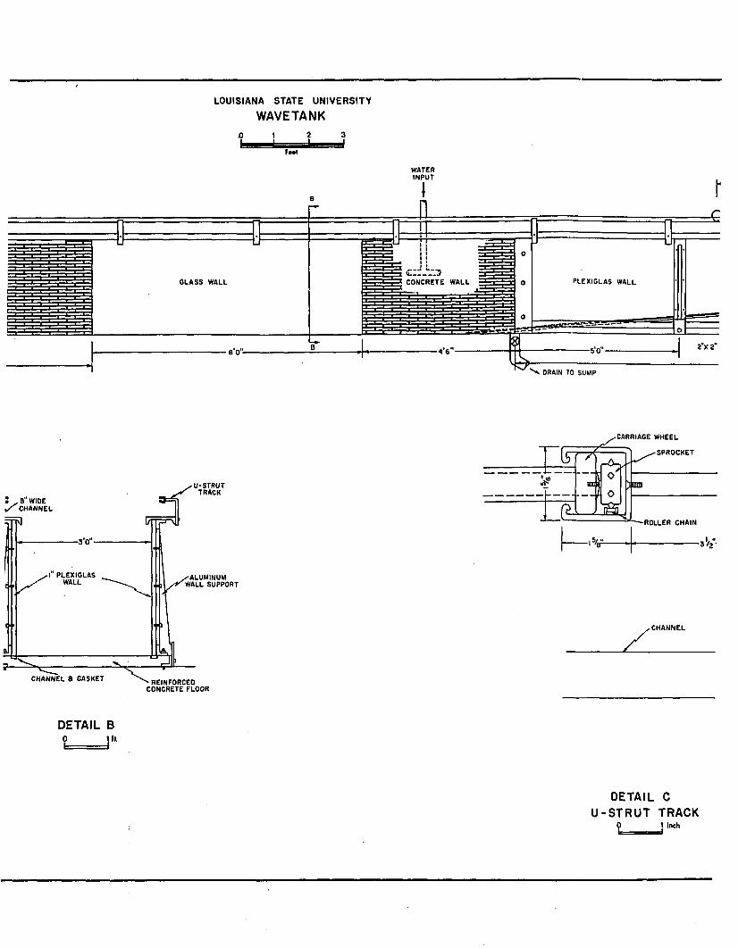
LOUISIANA STATE UNIVERSITY WAVETANK

WATERINPUT

PLEXIGLAS WALLGLASS WALL CONCRETE WALL

^ DRAIN TO SUMP

U-STRUTTRACK

5 . B1' WIDE CHANNEL

Trfa•3*0'

I PLEXIGLAS WALL

^ALUMINUM WALL SUPPORT

CHANNEL 8 GASKET v REINFORCED CONCRETE FLOOR

DETAIL B0 t = = J o.

CARRIAGE WHEEL

SPROCKET

} HOD

ROLLER CHAIN

V

..CHANNEL

z _ _____

DETAIL C U -S T R U T TRACK

0 1 inch

WATERINPUT

TOWINO CARRIAGEW' ALUMINUM

, PLATE

*/.“ ALUMINUM PLATE 'BEACH (SUBSTRUCTURE NOT SHOWN)

PO —PO PG CONCRETE WALL

MARINEPLYWOOD

2 "ANGLE (STEEL) 2aX2"ANGLE (ALUMINUM)4*6

20'0 '

NOTE: 69*0" TOTAL LENGTH98*10 WORKING SECTION

'TRACK SUPPORT

FIGURE 6

Figure 7. Overall view of the facility

8-

9 -

10-

1

Figure 8

At N /\\%

//

\y%

i

\ ni \ i \_ __i__\.

\ \

11 i10 11 12 13

pH

Free ion distribution in presence of the aluminum plate on the beach. (C = log molar concentration of ions in solution)

107

Figure 9. The wave generator. Baffles placed in frontand back of paddle serve as energy dissipators.

Figure 10. Sanborn Model 150 oscillograph

109%

input (6 VAC,1200c)

■V*”!300

brass rod probes Sanborn

Model 150

oscillator - recorder

- shield

12001000

output

N iC r wire probes

Figure 11. Schematic of Wheatstone bridge used with wave gauges.

imm

orsi

on

(fee

t)

OS'

03-

N o .l02-

No. 20.1-

0- -SWfc-

No.2-01-

WAVE METER N o.l-02-

-03-

-04--30 -25 -10 30-15

deflection (mm)

Figure 12. Wave gauge calibration curve

110

Y (d

epth

in

inch

es)

111

No. 2-1-S26 T ■ 1.0 soc. d0= 1.83 ft.

-0

-20-

- 3

- 4

- 5 -

-8

-86-

X, Horizontal Displacement (inches)t

Pig. 13. Mass transport in 1.0 second wave in thehorizontal floor section of tank (d=1.83 feet). Upper curves' represent water surface elevations corresponding to points on orbital path of particle (lower trace). Displacement of . particle is..toward beach.

Y (depth

in ii

112

No. 3 - 3 - S 4 2 T 1 1.0 ioc. d • 1.03 ft.

•o

12-

Boach Slope

X, Horizontal Displacement (inches)

Figure 14. Mass transport in shallow water wave for T=1.0 seconds and d=1.03 feet. Upper curves represent water surface elevation corresponding to points on orbital path of particle (lower trace) Displacement of particle is downbeach.

Y (depth

in inches)

113

No. 3 - 2 - S 4 2 T 1 1.25 j o c .

d • 1.03 fl.

0-

12-

Beach Stops

X, H orizontal Diiplacomonf (inchot)

Figure 15. Mass transport in shallow water wave for T=1.25 seconds and d=1.03 feet. Upper curves represent water surface elevation corresponding to points on orbital path of particle (lower trace). Displacement is downbeach.

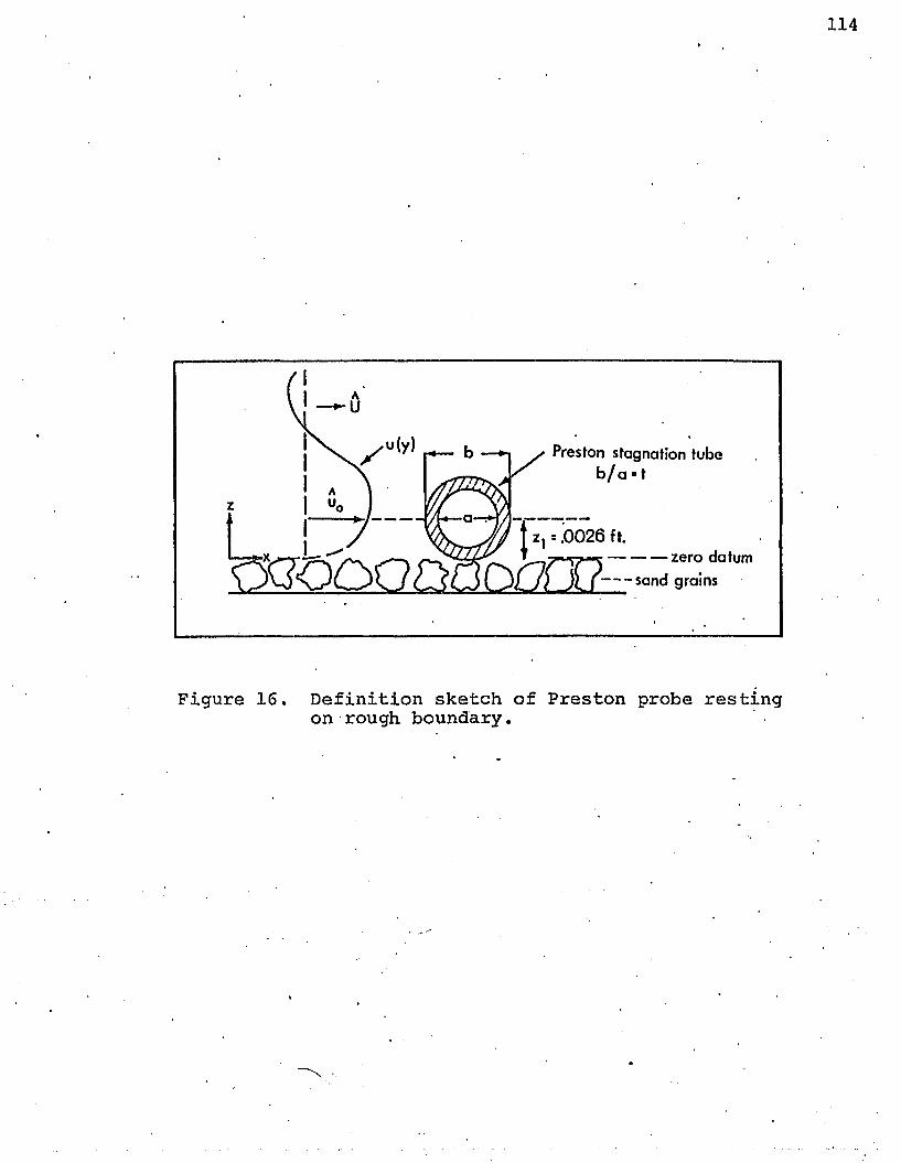
114

Preston stagnation tube b /a * t

Zj = .00 2 6 ft.~ zero datumO l 7 ) J l r — sqnd grains

Figure 16. Definition sketch of Preston probe resting on rough boundary.

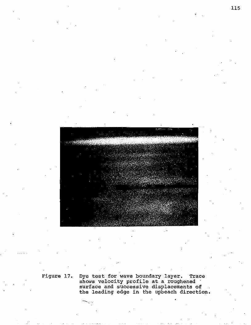
Figure 17. Dye test for wave boundary layer. Trace shows velocity profile at a roughened ' surface and successive displacements of the leading edge in the upbeach direction.

Figure 18. Experimental alignment of the Preston probe with a roughened beach slope. . The static probe is in front, the stagnation probe is . in the rear.

117

■ - n-coi>-v»

“i VmfllfffifttM--. ri

02*4*

W-Vy,

S f ^ K S f

Figure 19. Preston probe and wave gauge in test position

Pace

P9

0D

tran

sduc

er

r

Sanborn Model 150

oscillator - recorder

500£ 10KUioKn><-vw-

— shield

L

Figure 20. Schematic of the Pace pressure transducer.

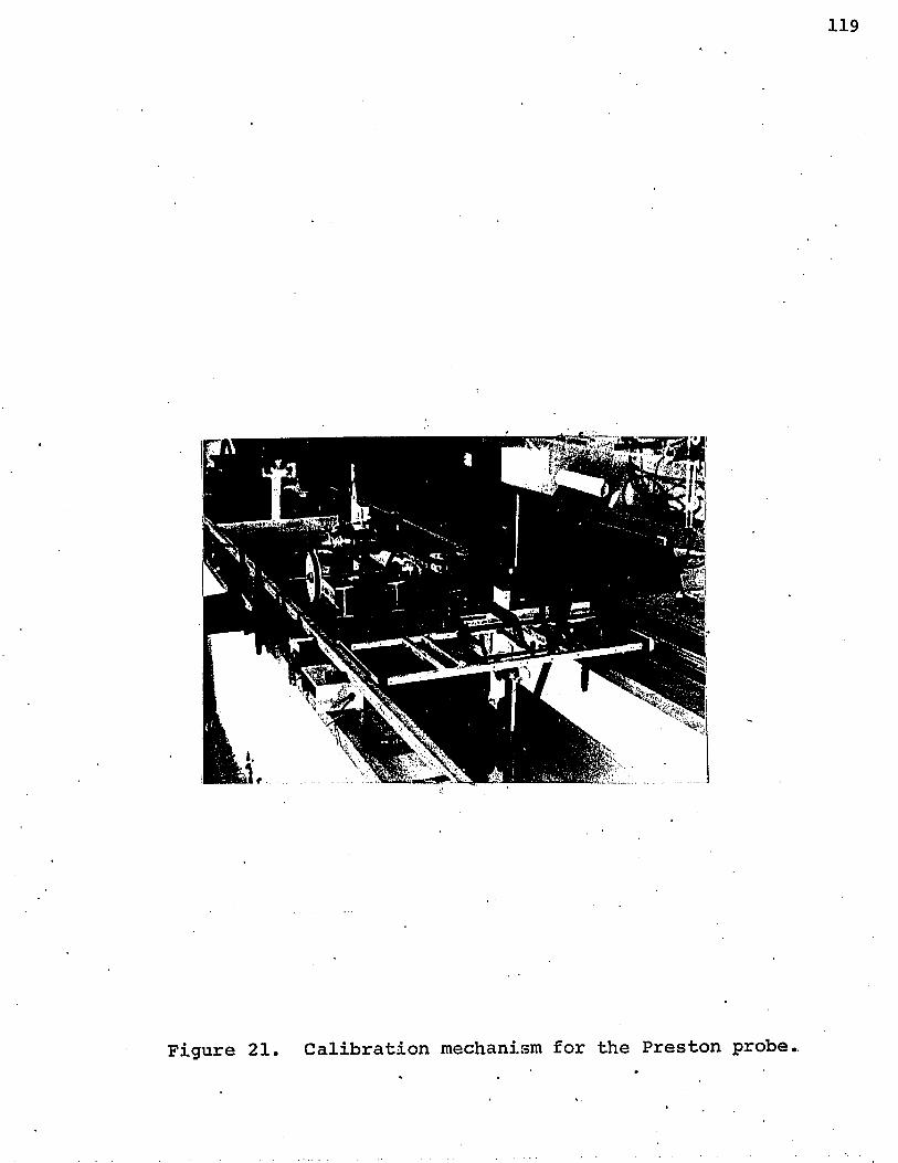
119

Figure 21. Calibration mechanism for the Preston probe

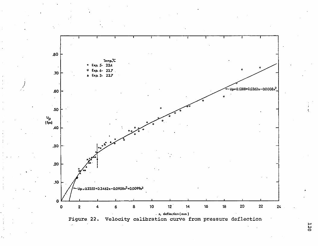
.80Temp^C

♦ Exp. 5 - 2 2 4

e Exp. 6 - 2 2 7

4 Exp. 3 - 23.7.70

Up* 0.1288+0.0362x- 0.0008x2_.60

.50

AO♦ O,

.30

.20

.10U p=0.2355+0.3462x-0 .0958x2+0.0099x?

20 2210 16 18124 8 14 240 2 6. x, deflection ( mm )

Figure 22. Velocity calibration curve from pressure deflection 120

Figure 23. Linearsyn differential transformer used in checking time lag in response of pressure measuring system. •

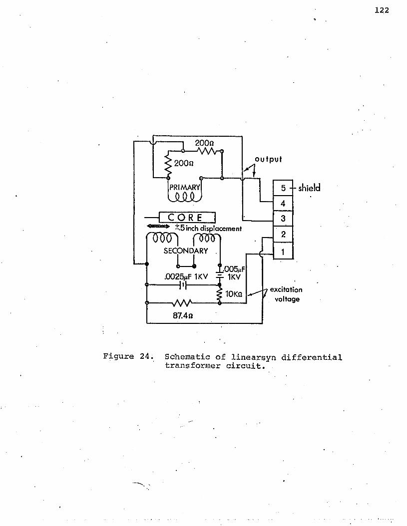
output

PRIMARYU L Q J U

— I C O R E Ii.5 inch displacementfTRRTl (W|

SECONDARY .

^ J1.005„F.0025juF 1KV 1KV

-W 10K1Ji >- VW-

87.4n

shield

excitationvoltage

Figure 24. Schematic of linearsyn differential transformer circuit.

0 R

AD

IAN

S

1.4

1.3

12

1.1

10 o&

.9

.8

225 2.5 2.751.75 201.0 1.25 1.5 aoT (SEC)

Figure 25. Time lag calibration curve for pressure measuring system.

Ap(

fps

x 10

'2)

100

1.2501.565 1.417 0.9171.0839 0

'Small" amplitude waves T (see.)

80

Largo" amplitudo waves

7 0

6 0

4 0

30

wave generation

4439 40 42 4536 37• x, distance up beach (ft.)

Figure 26, Pressure distribution in wave boundary ' layers on the "beach".

z(ft

-)

z (ft.)

1.0 sec.Smooth Boundary

» 5-39

'3 0 32 34 36 38 40 42 44 46

0* (fps x 10*)0225i-- 1 1 1 "i

T-1.0 sec.Smooth Boundary

Exp d (ft.) H(fU0 5*37 1.565 0.432• 5-39 1.417 0.4306 5-41 1250 0 .420a 543 1.083 0.417□ 545 0.917 0.423

49 47 37 35 33 3145 43 41 39

O' (fps x

Figures 27-28. Near bottom experimental velocity profileson sloping1 beach, corresponding to wave crests (at=0, upper diagram) and wave troughs (at=ir, lower diagram). Test series 5, T=1.0.

z (ftJ

z (ft.)

.0225

.0200

.0175

.0150

.0125

.0100

.0075

.0050

0025

0

.0225

.0200

.0175

.0150

.0125

.0100

.0075

.0050

0025

0

T> 1.5 sec.Smooth Boundary

Exp d(ft.) H(fOo5-37 1.565 0.258o 5-39 1.417 0.267

. a 5-41 1.250 0.265a 5-43 1.083 0268□ 5-45 0.917 0.265

_— □— j—*.-- r

30 32 34 36 38 40 42 44 46 48 50 52 54

U* (fps x IQ'2)

T» 1.5 sec.Smooth Boundary.

Exp d(ft.). H(ftJ

o5-37 1.565 0.275• 5-39 1.417 0.275a 5-41 L250 0.278a 543 1.083 0.283o545 0.917 0.268

55 53 51 49 47 45 43 41 39 37 35 33 - 310" (fps x

Figures 29-30. Near bottom experimental velocity profileson sloping beach. Test series 5, T=1.5, •a t=0 f' If m

2 Wt

J Z

(ft.)

127

38 40 42 44

0*(fpS X 10-2)-A-

T*2.0sec.Smooth Boundary

Exp d(ft.) H(fUo5-37 1.565 0.169o5-39 1.417 0.181a 5-41 L250 0.203a 543 1.083 0.185o 5-45 0.917 0.196

.

T* 2.0 sec.Smooth Boundary

Exp- dlft.)0.4690.181

o5-37 1.565o5-39 1.417a 5-41 1.250 0.203a 5-43 1.083 0.185o 545 0.917 0.196

46 48 50

A •

— t--------52 54

55 53 51 49 47~ 45 43. . 41 39 37 35 8 3 “ W

0”(fps x 10-2)

Figures 31-32. Near bottom experimental velocity-profileson sloping beach. Test series 5, T=2.0,at=0,n.

Z (ft.)

Z (ft.)

.0225

.0200

.0175

.0150

.0125

.0100

.0075

.0050

0025

0

Ttl.O sec.Smooth Boundary

Exp d(ft.) H(ft.)o6-37 1.565 0.228o&-39 1.417 0.216a 641 1.250 0.205a 643 1.083 0.202o645 0.917 0.225

/

10 12 14 16 18 20 22 24 26

O'lfps x 10*)

28 30 32 34

.0225

T«1.0sec Smooth Boundary

Exp d(ft.) H(ft)o6-37 1.565 0.228o6-39 1.417 0.216a 6*41 L250 0.205a 643 1.083 0.2020 6-45 0.917 0.225

.0200

.0175

.0150

.0125

.0100

.0075

0050

0025

Figures 33-34. Near bottom experimental velocity profileson sloping beach. Test series 6, T=1.0,crt=0, ir.

z (f

t)

z (f

t.)

129

“■1.5sec.Smooth Boundary

.0225

.0200

.0175

.0150

.0125

.0100

.0075

.0050

0025

010 12

29 27 25 23 21O' (fps x 10-*)-t. r

15 13

1 --------r-T*1.5sec.Smooth Boundary

Exp d(fU H(ftl

o6-37 1.565 0.135• 6-39 1417 0.128*6-41 1.250 0.146*6-43 1.083 0.137o6-45 0.917 0.128

20 22 24

0*(fps x 10*)

26 28 30 32

Figures 35-36. Near bottom experimental velocity profiles on sloping beach. Test series 6, T = 1.5, a t=0, ttN

Z (ft.)

2 (ft

.)

.0_v5

.0200

.0175

.0150

.0125

.0100

.0075

.0050

0025

0 ,

qzr

.0225

.0200

.0175

.0150

.0125

.0100

.0075

.0050

0025

0

AA»

- r ' f t *

T* 20 sec.Smooth Boundary

— Exp d(ft.) H(ft.)o6-37 1.565 0.075o6-39 1.417 0.073a 6 41 1.250 0.070a 6-43 1.083 0.077°6 4 5 0.917 0.082

_l________ I________ I________ I________ L.10 12 14

U'(fps x 10-J)

16 18 20 22 24

T>2.0sec.Smooth Boundary

Exp d(ft.) H(ft.)

o6-37 1.565 0.075o6-39 1.417 0.073a 6-41 1.250 0.070a 6-43 1.083 0.077o6-45 0.917 0.082

35 33 31 29 27

Q #

1125 23 21 19

ih fp s x H W

Figures 37-38. Near bottom experimental velocity profileson sloping beach. Test series 6, T=2.0,at=0, tr.

z (ft

.) z

(ft.)

131

T* 1.0 sec.Rough Boundary

Expi d(ft.)o7-37 1.565 0.429°7-39 1.417a 7-41 1.250 0.410a 7-43 1.083 0.413o 7-45 0.917

'30 32 34 36 38 40 42 44

0*(fps x 10*)

48 50 52 54

.0225T- l.Osec.Rough Boundary

Exp dftU H(ft)o7-37 1.565 0.429o7-39 1.417 0.416a 7-41 L250 0.410a 7-43 1.083 0.413o 7-45 0.917 0.412

.0200

.0175 Ok

.0150

.0125

.0100

.0075

.0050

0025

Figures 39-40. Near bottom experimental velocity-profileson sloping beach. Test series 7, T=1.0at=0, it.

Z (ft

.) 2

(ft.

)

132

.0225

.0200

.0175

.0150

.0125

.0100

.0075

.0050

0025

0

T* 1.5 sec.Rough Boundary

Exp d (ft.) H(ft)o7-37 1.565 0.265o7-39 1.417 0.269a 7-41 1.250 0.242*7-43 1.083 0.278a 745 0.917 0.264

30 32

.0225

.0200

.0175

.0150

.0125

.0100

.0075

£050

0025

0

34 40 42 44 46

0* (fps x 10-*)

48 50 52 54

A A O

T'1.5 sec.Rough Boundary

Exp' d(ft.) H(ftJ

o7-37 1.565 0.265o7-39 1.417 0.269*7-41 1.250 0.242*7-43 1.083 0.278□ 745 0.917 0.264

*>5 53 51 49 47 45 43 41 39 37 35 33 31

O'(fps x i o * )

Figures 41-42. Near bottom experimental velocity profileson sloping beach. Test series 7, T = 1.5,at=0, it.

z (ft.)

Z (ft.)

133*

.0225

.0200

.0175

.0150

.0125

.0100

.0075

.0050

0025

°2 0 2 2 24 26 28 30 32 34 3 6 38 40 42 440* (fps x 10-a)

.0225 " ‘ ------------------------------ ------------------------ ------------ -----------------—

.0200

.0175

.0150

.0125

.0100

.0075

.0050

0025

0 51 49 47 45 43 41 39 37 35 33 31 29 27

0" (fps x 10*)

Figures 43-44. Near bottom experimental velocity profileson sloping beach. Test series 7, T = 2.0, o t=0, t t .

T» 2.0 sec.Rough Boundary

Exp d(ft.) H(ftJo7-37 1.565 0.169o7-39 1.417 0.183a 7-41 L250 0.182a 7-43 1.083 0.180□ 745 0.917 0.177

T

AO

I Il

T-2.0 sec.- Rough Boundary

Exp d(ft.) H(ft.)* o7-37 1.565 0.169

o7-39 1.417 0.183a 7-41 1.250 0.182

- a 7-43 1.083 0.180□ 7-45 0.917 0.177

z (ft

.) z

(ft.

)

.0225T> 1.0 sec.Rough Boundary.0200Exp d(ft.) H(ft.)

o8-37 1.565 0.207•8-39 1.417 0.199a 8-41 1.250 Q200a 8 43 1.083 0.217o8-45 0.917 Q200

.0175

.0150

.0125

.0100

.0075

.0050

0025 —V-

U‘ (fps x 10*)

.0175

.0150

.0125

.0100

.0075

.0050

0025

• 0 41 39 37 35 33 31 29 27 25 23 21 19IT (fps x 10*)

-

T» 1.0 sec.Rough Boundary

Exp d (ft.) H(ft)o8-37 1.565 0.207•8-39 1.417 0.199a 8-41 1.250 0.200*8-43 1.083 0.217q 8-45 0.917 0.200

i 1 fn---------- r< -Y — r

\

Figures 45—46. Near bottom experimental velocity profiles on sloping beach. Test series 8, T = 1.0, o t=0 , it .

z (ft

.) Z

(ft.

)

.0225

T> 1.5 sec.Rough Boundary

.0200Exp dlft.) H(ft.)

o8-37 1.565 0.131•8-39 1.417 0.115*8-41 1.250 0.125a 843 1.083 0.139□ 8-45 0.917 0.124

.0175

.0150

.0125

.0100

.0075

.0050

0025

.0225

.0200

.0175

.0150

.0125

.0100

.0075

.0050

0025

0

T> 1.5 sec.Rough Boundary

Exp d(ft.) H(ft)o8-37 1.565 0.131•8-39 1.417 0.115a 8*41 L250 0.125A 8-43 1.083 0.139o8-45 0.917 0.124

43 41 39 37 35 33 31 29 27 25 23 21 19

U"(fps X 10-2)

Figures 47-48. Near bottom experimental velocity profileson sloping beach. Test series 8, T = 1.5,ot=0, ir.

z (ft

.) z

(ft.

)

.0225

.0200

.0175

.0150

.0125

.0100

.0075

.0050

0025

0 0 2 4 6 8 10 12 14 16 18 20 22 24O' (fps x M H

.0225

.0200

.0175

.0150

.0125

.0100

.0075

.0050

0025

°3 4 32 30 28 26 24 22 20 18 16 14 12 10

(W fpsxlO-*)

Figures 49-50. Near bottom experimental velocity profileson sloping beach. Test series 8, T = 2.0, ot=0, ir.

T« 2.0 sec.Rough Boundary

Exp d(ft.) H(fUo8-37 1.565 0.071o8-39 1.417 0.072a 8-41 1.250 0.070A 8*43 1.083 0.0720 8-45 0.917 0.079

— i—

V v .

T12.0 sec.Rough Boundary

Exp dlft.) H(ft.)

o8-37 1.565 0.071o8-39 1.417 0.072a 8-41 1.250 0.070a 8 43 1.083 0.072o8-45 0.917 0.079

137

45

-20

550 degrees

65 75 85 05 70 800 degree!

90 100 110 120

.060

r 1 1 ... 11 = 2.0 d0> 2.000 (ft) .060

I ... 1 1T = 2.0 <fc?000{fO

Experiment d H Experiment d HO 8-37 1.562(ft) 0.07l(ft) o 6-37 1.562 (ft) OQ75(ft)a 0-39 1.417 0.072 a 6-39 1.417 0.073

055 a 8-41 1.250 0070 _ .055 _ o 6-41 1.250 Q070 -a 8-43 1083 0072 a 6-43 1.083 0.077n 8*45 0917 0079 o 6-45 0.917 0082

.050 - - .050 - -

3045 — .045

"

.040 - .040 - -

.035 - - .035 -

vd.030 - - .030 — A -

A

.025 - 3 “ .025 - 3

A.020 - — .020 — -

3 □•

A - * A.015 - - .015 ~ (►

3 • • OA A

o 4 A O.010 — • .010 — •

A A□ o O O

A A• •

.005 — A O “ .005 - A -O

•□0o A 0A • O

n 1 1 1 n 1 1 1-10 ' 0 10

0 degrees

20 30 -20 -10 0 10 0 degree!

20 30

Figures 51-52. Phase distribution of Uq /u with depth on smooth bottom (test serxes 6).and rough bottom (test series 8) for small amplitude waves. Upper scale shows deviation from surface history, lower scale refers to boundary layer.

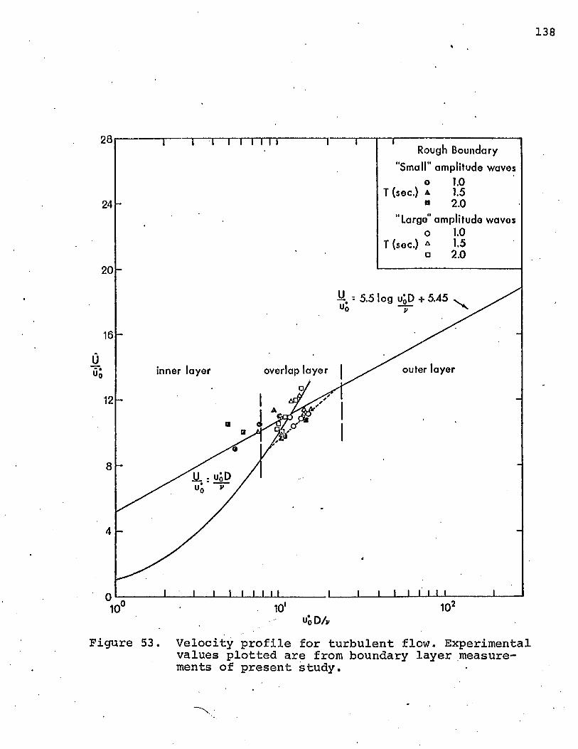
138

28Rough Boundary

"Small" amplitude waveso 1.0

T (sec.) a 1.5" 2.0

“Large" amplitude wavos o 1.0

T (sec.) a 1.5□ 2.0

24

20

AA : 5.5 log UqD + 5.45

16

outer layeroverlap layerinner layero12

8

4

0 ,0 10'10UqD/v

Figure 53. Velocity profile for turbulent flow. Experimental values plotted are from boundary layer measure­ments of present study.

X

10'

M .

xoE

10'

10'

i 1 r 1----1---- 1— :— i--- 1 r

d (ft.)> i.5 6 5 . 1.417 1.250 1.003 0.917

Smooth Boundary T (soc.) o - 1.0

a - 1.5 d - 2 .0

Rough Boundary o - 1.0

* - 1 . 5 a - 2 .0

op

o>So"Oa6a

oE<n

©>o©"O3

. / /

/

iiiqI i

q| «o!cnI ^:l JLl ill

/

w avo generation

It tH 1 L _L X X X36 3 7 38 39 4 0 41 42 43 44

(distance up beach, ft.)45

I I I JI 1 1

1 1I iizo ne of breaking wavesi i i

1 ! 1i i ii i i

—\—i— — i--- !— L_48 4 9 5 0 51

Figure 54. Shear stress distribution up beach' for smooth and rough boundaries and at=0.

1 0 J

xDE

10'

10'

d ( f l . ) ‘ 1.565 1.417 1.250 1.083 0.917

a.

<

to

Smooth Boundary T (sec.) o - 1.0 a - 1.5 a - 2.0

Rough Boundary o - 1.0

a - 1.5

a - 2.0

III P

w ave generation

1 L X X X36 37 38 39 4 0 41 42 43 44

(distance up beach, f».)

45

I Ipj mjcn I I

A 1 I I JI Ii 1 1I I I

zone of breaking w avesi i iI I II I JI I II !

- V _L48 49 50 51

Figure 55. Shear stress distribution up beach for smooth and rough boundaries and. ot=ir

omax

(ib

./ft?

x

10-3)

141*

10'1Smooth Boundary

T (sec.). o 1.0

a 1.5

o 20 Rough Boundary

o 1.0 a 1.5 a 2.0

10“

"i— I— i i r r r t 1--- 1— i— i— i i r

"Lorgo” amplitude waves

/w.o.□

'Small" amplitude waves

■▲■

* i i i i i i i I i I__I— I I 1.1-2 10- '

H10°

XIFigure 56. Relation between the amplitude of the

maximum boundary shear stress and relative wave height for dt=0

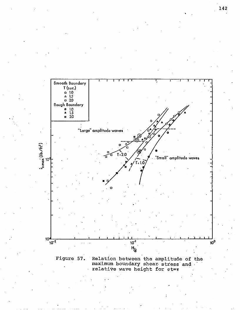
142

Smooth Boundary T (soc.) o 1.0 a 1.5 a 2.0

Rough Boundary

Largo" amplitude waves

7/0

—

• "Small" amplitudo waves/-"■ - ./ T = 1.0

H.

Figure 57. Relation between the amplitude of the maximum boundary shear- stress and - relative wave height for ot=ir

Smooth Boundary Experiments (see.) H0(fj.)

'larQ«* amplitude wavot o IX) .480* 15 .2840 _ 2X5 .200

'Small* amplitude waves -o • TX) - 2 2 H _

* 1.5 J3S* ' 2X5 X>75

So

a'

^i^ure 58. Relation between friction factor Cf and the R e y n o l d s

number for smooth, surfaces. . Solid line is Kajiura's (1968) expression.

144

10'

■ M-•u

----------- 1 .......1 "1----- 11 I 1 | - T ,Rouah Boundary

- ExporimonM- T (soc.) H0 (ft.)

- "Largo” amplitude wavos

o 1.0 ,441A 1.5 .2610 2.0 .179

"Small" amplitude wavoje 1.0 .207a 1.5 .133

\ \ « u 2.0 065Zo-.00123 ft.

10

J 1 I l ■ I I I I I i l i t l____I___I__I__I I — I— 1— L-103 • 10^R = UP

¥

104

Figure 59. Relation between friction factor and Reynolds number IRj for roUgh surfaces.

145

Table 1. Example of calculated wave parameters for increments of z.

Exp=5, Station=45, do=2.000 ft., d=0.917 ft., Temp«73.22‘7P, Stroke=0.5 42 ft.

Smooth boundaryT=1.0 sec., Ho=0.570 ft., L=4.93 ft., L =5.44 ft., d/L=0.186

L/Lq=0.906No. z (ft) H (ft) H/H0 H/d H/T210 . 0026 0. 400 0.702 0. 436 0. 40020 .0076 0. 449 0.788 0. 489 0.44930 .0126 , 0.412 0. 72 3 0. 449 0. 41240 .0176 0.439 0.770 0.479 0. 43950 .0226 0. 439 0.770 0.479 0. 43960 .0426 0.445 0.646 ■ 0. 485 0.44570 .0626 0. 368 0. 781 0. 401 0. 368sec, Ho=0.2 80 ft, Lq== 9,.36 ft. •

00IIl-q 91 ft.,L/Lo=0.952.10 .0026 0.267 0.953 0729T 0.11920 .0076 0.297 1.061 0. 324 0.132 .30 .0126 0.252 0.900 0.275 0.11240 .0176 0.256 0.914 0 ‘. 2 79 0.11450 .0226 0.240 0. 857 0.262 0.10860 .0426 0.284 1.014 0. 309 0.12670 .0626 0.283 1.011 0. 309 0.126

T=2.0 sec, •oII0w 205 ft. , Lq=13.4 8 ft. , L= 12.67 ftd/L= 0.072, L/Lo=0.9 3910 .0026 0.191 0.932 0.208 0.04820 .0076 0.191 0.9 32 , 0.208 0.04830 .0126 0.222 1.082 0.242 0.05540 .0176 0.192 0.9 36 0.209 0.04850 .0226 0.190 0.927 0.207 0.04860 .0426 0.126 0.907 0.203 0.04770 .0626 0.186 0.907 0.203 0.047

146

Table 2. Experimental values of velocity, pressure and phase lag for increments of z.

Ixp-Sta-No. U)25

(ft.)(2)

de f 1. (mm)

(3) (4)U AP -9 (fpsxlO ■‘)(fpsxl0 *)

' (5)0(rad)

(6)0

(deg)’=1.0 sec.5-37-■10 .0026 8.0 36.719 13.045 2.38 136.36

20 .0076 7.50 35.529 12.213 - —30 .0126 7.35 35.165 11.964 1.40 80.2140 .0176 7.55 35.651 12.297 1. 44 82.5050 .0226 6.56 33.184 10.654 2.79 159.8560 .0426 6.6 33.287 10.720 ' 1.42 81.3670 .0526 6.7 33.543 10.885 . 1.48 84.79

’=1.5 sec. .5-37-•10 .0026 9. 32 39.669 15.225 1.81 103.70

20 .0076 10.6 42.263 17.2 81 2.01 115.1630 .0126 . 8.82 38.585 14.404 0.50 2 8.6440 .0176 8.5 37.869 13.875 1.55 88.8150 .0226 11.2 43.389 18.214 2.25 128.9160 .0426 8.1 36.953 13.211 1. 88 107.7170 .0526 7.2 34.796 • “11.715 1.21 69.32

’=2.0 sec.5-37-■10 .0026 6.18 32.19 6 10.029 1.77 101.41

20 .0076 9.5 , 40.049 15.519 2.27 130.0630 .0126 6.55 33.159 10.638 .32 18.-3340 .0176 7.0 34.299 11.382 - -50 .0226 7.8 36.248 12.713 1.64 93.9660 .0426 6.1 • 31.985 9.898 1.12 64.1770 .0526 ' 5.9 31.453 9.571 1.64 9 3.46

147

Table 2. Experimental values of velocitypressure and phase lag for increments of z.

(continued)

(1) (2) (3) (4) (5) (6)Exp-Sta-No. z defl. U Ap 0 0

(ft.) (mm) (fpsxlO ) (fpsxlO ) (rad) (deg)T=1.0 sec •

5-39-10 .0026 8.67 ’ 38.252 14.156 1.37 78.4920 .0076 9.04 39.067 14.766 2.14 122.6130 .0126 8.9 38.761 14.536 1.57 89.9540 .0176 7.8 36.249 12.713 1.07 61. 31-50 .0226 8.0 36.719 13.045 1.52 87.0960 .0426 7.65 35.891 12.463 1.22 69.9070 .0526 8.0 36.719 13.045 1.24 71.05

T=1.5 sec •

5-39-10 .0026 11.1 43.205 18;060 1.99 114.0120 .0076 10. 85 42.739 17.673 1. 88 107.7230 .0126 10.4 41.875 16.965 2.09 119.7540 .0176 9.6 •20.259 15.681 1.67 95.6850 .0226 10. 87 42.777 17.704 2.09 119.7560 .0426 8.75 38.429 14.289 1.04 59.5870 .0526 8.55 37.983 - -13.95.8 1.88 107.72

T=2. 0 sec •

5-39-10 .0026 11.1 43.205 18.060 1.70 97. 4020 .0076 9.45 39.995 15.437 2.59 148.3930 .0126 10.55 42.167 17.202 2.59 148.3940 .0176 6.4 32.771 10.390 1.22 69.950 .0226 6.77 33.721 11.001 1.96 112.2960 .0426 ,5.5 30.369 8.923 1.11 . 113.44

. 70 .0526 5.8 31.185 9. 409 1.61 92.25

148

Table 2. Experimental values of velocity,pressure and phase lag for increments of z.

(continued)

(1) (2) (3) (4) (5) (6)Exp-Sta-No. z defl. U Ap „ 6 e

(ft.) (mm) (fpsxlO-'2) (fpsxlO ) (rad) (deg)T=1.0 sec.5-41-10 . 0026 12.6 45.791 20.287 1.28 73. 3420 .0076 12.05 44.885 19.492 1.29 73.91

30 .0126 10. 3 ' 41.679 16.807 1.22 69.9040 .0176 10.6 42.263 17.281 1. 30 74. 4850 . 0226 11. 4 43.751 18.519 1. 82 104.2860 .0426 10.2 41.481 16.647 1.29 73.9170 .0526 9.82 40.714 ■ 16.037 1.19 68.18

T=1.5 sec.5-41-10 .0026 13. 3 46.875 21.258 0.25 14. 32

20 .0076 11. 8 44.457 19.122 1; 47 84.2230 .0126 11.8 44.457 19.122 1.59 91.1040 .0176 11.13 43.260 18.106 1.09 62.4550 .0226 14.4 48.419 22.682 1.54 88.2360 .0426 11.9 44.629 19.270 0. 41 23. 4970 .0526 11.0 43.019 . -17.906 0.78 •44.69

T=2.0 sec.5-41-10 .0026 8.1 36.953 13.211 2.15 123.18

20 .0076 8.0 36.719 13.045 2. 71 155.2730 .0126 7.9 36.485 12.879 2.53 144.9640 .0176 6.7 33.542 10.885 2.65 151.8350 .0226 9.7 40.467 15.843 2.65 151.8360 .0426 7.8 36.488 12.713 1. 39 • 79.6 470 .0526 6.8 33.797 11.051 1. 49 85. 37

149

Table 2. Experimental values of velocity,pressure and phase lag for increments of z.

(continued)

(1) (2) (3) (4) (5) (6)Exp-Sta-No, z def 1. U Ap 0 0

(ft.) (mm) (fpsxlO- )(fpsxlO ) (rad) (deg)T=1.0 sec.5-43-10 .0026 9. 85 40.775 16.086 1.093 62.62

20 .00 76 12. 35 45.385 ' 19.929 1.013 58.0430 .0126 12.95 46.343 20.778 1.113 6 3.7740 • .0176 13.2 46.725 21.122 1.063 60.9050 .0226 13. 42 47.053 21.420 1.193 68. 3560 .0426 12.55 •45.711 20.216 1.32 75.6370 .0526 13. 3 46.875 21.258 1. 32 . 75.63

T=1.5 sec.5-43'-10 .0026 13. 7 '47. 459 21.791 0.54 30.94

20 .0076 14.45 48.485 22.744 -0.0496 - 2.8430 .0126 14. 3 48.287 22.558 0. 37 21.1940 .0176 13. 8 47.601 21.922 0. 33 18.9150 .0226 18.6 52.535 26.702 0.1304 7.4760 .0426 14. 3 48.287 22.558 0.21 12.0 370 .0526 13.6 47.315 • •21.659 0.21 12.0 3

’=2.0 sec.5-43--10 .0026 9. 85 40.775 16.086 0.41 23.49

20 .0076 9.95 40.979 16.247 0.449 25. 7230 .0126 9.95 40.979 16.247 0. 449 25. 7240 .0176 9.9 40.877 16.166 0. 319 18.2850 .0226 ID. 1 41.281 . 16;487 0. 819 46.9260 .0426 9. 85 40.775 16.086 0.51 29.2270 .0526 8.8 38.541 14.371 0. 70 40.11

150

Table 2< Experimental values of velocitypressure and phase lag for increments of z.

(continued)

Ejp- Sta-No (1)z

(ft.)(2)

def 1. (mm)

(3)U _ 2(fpsxlO )

(4)AP -o (fpsxlO ')

(5)9

(rad)(6)6

(deg)T=1.0 sec.5-45 -10 .0026 19.4 52.999 27.176 0.903 51.74

20 .0076 17.8 51.969 26.129 0.633 36.2730 .0126 18.0 52.120 26.282 0. 834 47. 7840 .0176 18.0 52.120 26.282 0. 873 50.0850 .0226 17.6 51.811 25.971 0.653 37. 4160 .0426 18.5 52.465 26.636 0. 848 48.5970 .0526 16.5 50.830 24.997 0. 823 47.15

T=1.5 sec.5-45'-10 .0026 17.5 51.730 25.890 -0.0596 - 3. 41

20 .0076 15.7 49.995 24.182 0.6204 35.5530 ' .0126 18.15 52.229 26.392 -0.1096 -6.2840 .0176 15. 8 50.105 24.289 0.7204 41.2 850 .0226 16.7 51.023 25.187 0.37 21.1960 .0426 20.0 53.280 27.465 0.2054 11. 7770 .0526 18.2 52.265 • -26.42 8 0.1904 10.91

T=2.0 sec.5-45--10 .0026 11.65 44.195 18.897 0.259 14. 84

20 .0076 9.8 40.643 16.005 0.259 14.8430 .0126 11.5 43.929 18.671 0.239 13.6940 .0176 10.8 42.645 17.595 0.0098" .5650 .0226 10.3 41.678 16.807 0.229 13.1260 .0426 11.4 43.751 18.519 0.369 21.1470 .0526 9.62 40.301 15.714 -0.255 --14.61

151

Table 2. Experimental values of velocitypressure and phase lag for increments of z.

(continued)

Exp-Sta-No (1)z

(ft.)(2)

defl.(mm)

(3) (4)U _2 Ap

(fpsxlO ) (fpsxlO-'*)(5)

. . 0 (rad)

(6)0

(deg)T=1.0 sec. •

5-37-11 .0026 9.0 38.979. 14;700 -0.63 -36;0921 .0076 9.26. 39.541 15.127 -0.692 -39.6531 .0126 9.2 39.413 15.029 • — ~

41 ' .0176 9.15 39.305 14.947 -0.628 -35.9851 .0226 10.9 42.833 17.750 -0.666 -38.16

T=1.5 sec.5-37 -11

21314151

. 0026

.0076

.0126

.0176

.0226

10.49.0

10.010.29.4

41.875 38.979 41.079 41.481 39.839

16.965 14.700 16.327

• 16.647 15.356

-0.422 -24.18 -0.799 -45.78-0.422 -24.18 -0.841 -48.18

T=2.0 sec.5-37 -11 .0026 7.2 34.797 11.715 -0.336 -19.25

21 .0076 7.4 35.287 ■ -12.047 -0.631 -36.1531 .0126 7.45 35.409 12.130 - -

41 .0176 7. 45 35.409 12.130 -0.502 -28.7651 .0226 7.46 35.433 12.147 -0.499 -28.59

152

Table 2. Experimental values of velocitypressure and phase lag for increments of z.

(continued)

Exp-Sta-No(1)z

(ft.)(2)

def 1. (mm)

(3) (4)U -2 Ap -2 (fpsxlO z ) (fpsxlO )

(5)0

(rad)(6)0

(deg)T=1.0 sec.5-39-11 .0026 11.2 43.389 18.214 -0.19 -10.89

21 .0076 9.9 • 40.877 16.166 -0.692 -39.6531 .0126 11.02 43.057 17.937 -0.21 -12.0341 ■ .0176 12.2 45;137 19.711 -0.475 -27.2151 .0226 12.5 45.629 20.144

T=1.5 sec.5-39-11 .0026 10.0 41.079 16.327 -0.71 -40.68

21 .0076 10.62 42.302 17.313 -0.885 -50.7131 .0126 10.0 41.079 16.327 -0.925 -52 .9941 . 0176 10.62 42.302 17.313 -0.841 -48.1851 .0226 10.4 41.875 16.965 -0. 84 -48.13

T=2.0 sec.5-39-11 .0026 7.42 35.335 12.080 -0.65 -37.24

21 .0076 9.17 39.348 “14.979 -0.399 -22.8631 .0126 8.06 36.860 13.145 -0.415 -23.7841 .0176 8.28 37.369 13.510 -0.556 -31.8651 .0226 8.0 36.719 13.045 -0.556 -31.86

153

Table 2. Experimental values of velocitypressure and phase lag for increments of z.

(continued)

(1) (2) (3) (4) (5) (6)Exp-Sta-No z defl. U o ' Ap - 0 0

(ft.) (mm) (fpsxlO ) (fpsxlO ) (rad) (deg)T=1.0 sec.5-41-1.1 .0026 16.72, 51.042. • 25.206 -0.44 -25.21

21 . 0076 .15'. 7 ' 49.995 24.182 -0.09 r 5.1*5. 31 .0126 17.6 51.811 25.971 -0.504 -28.8941 .0176 16.1 50.425 24.601 -0.-482 -27,6251 .0226 18. 86 52.697 26.867 -0.384 -22.00

T=1.5 sec.5-t41-ll .0026 11.9 44.629 . 19.270 -0.747 -42.79

21 .0076 10.9 42.833 17.750 -0.422 -24.1831 .0126 11.4 43.751 18.519 -0.632 -36.2141 .0176 11.48 43.894 18.641 -0.422 -24.1851 .0226 11.6 44.107 18.822 -0.557 -31.91

T=2.0 sec.5-41-11 .0026 9.6 40.259. 15.6 81 -0.711 -40.74. . 21 .0076 9.4 39.839 . .15. 356 -0.711 -40.74

31 .0126 8.4 37.643 13.709 -0.615 -35.2441 .0176 8.74 38.408 14.274 -0.493 -28.2551 .0226 7.8 36.2 49 12.713 -0.451 -25.84

154

Table 2. Experimental values of velocitypressure and phase lag for increments of z .

(continued)

(1) (2) (3) (4) (5) (6)Exp-Sta-No z defl. U .9 Ap 0 6

(ft.) (mm) (fpsxlO ) (fpsxlO ) (rad) (deg)

■-3 II H* • o sec •

5-43--11 .0026 20. 7 53.535 2 7.72 8 -0.4 -22.9221 .0076 2.16 53.747 27.949 -0.335 -19.1931 .0126 25.1 53.341 27.528 -0.565 -32.3741 .0176 18.4 52.403 26.568 -0.749 -42.9151 .0226 25.0 . — mm -0.692 -39.65

T=1.5 sec •

5-43--11 .0026 16.9 51.209 25.371 -0.516 -29.5621 .0076 15.6 49.883 24.075 -0.32 -18,3331 .0126 14.4 48.419 22.682 -0. 306, -17.5341 .0176 15.2 49.421 23.630 -0.446 -25.5551 .0226 14.4 48.419 22.682 -0.13 - 7.45

T=2 . 0 sec •

5-43-■11 .0026 13. 3 46.875 21.258 -0.58 -33.2321 .0076 11. 8 44.457 . -19.122 -0.404 -23.1531 .0126 12.25 45.219 19.784 -0.452 -25.8941 .0176 11.63 44.160 18.867 -0.242 -13.8651 .0226 11.8 44.457 19.122 -0.43 “24.63

155

Table 2. Experimental values of velocitypressure and phase lag for increments of z.

(continued)

(1) (2) (3) (4) (5) (6)Exp-Sta-No Z ' def 1. U AP -2 0 0

(ft.) (mm) (fpsxlO ) (fpsxlO ) (rad) (deg)T=1.0 sec.5-45-11 .0026 27.1 52.229 • 26.392 -0.709 40.'62

21 .0076 23.9 53.701 27.901 -1.006 -57.64-31 .0126 23.6 53.755 27.957 -0.58 -33.2341 .0176 22. 3 5 3.82 3 28.027 -0.335 -19.1951 .0226 22.6 53.831 28.036 -0.50 -28.6561 .0426 24.6 53.519 27.712 +0.45 25-. 7871 .0526 29. 4 50.159' 24.342 -0.25 -14.3281 .0626 25.5 53.170 27.352 -0.13 - 7.45..

T=1.5 sec.5-45-11 ■ .0026 12. 3 45.303 19.856 -0.23' -13.18

21 ..0076 19. 4 52.999 27.176 -0.547 -31.3431 .0126 18.65 52.567 26.735 -0,495 -28.3641 .0176 18. 85 52.691 26.861 -0.442 -25.3251 .0226 16.0 50.319 . 24.498 -0.129 - 7.3961 .0426 18.6 52.535 -26.702 -0.229 -13.1271 . .0526 19. 4 52.999 27.176 -0.152 - 8.7181 .0626 19.5 53.050 27.228 -0.305 -17.47

T=2..0 sec.5-45-11 .0026 15.61 48.894 24.085 -0.399 -22:86

21 .0076 13.0 46.419 20.847 -0.242 -13.8631 .0126 12.9 46.265 20.709 -0.305 -17.4741 .0176 15.2 49.421 23.630 -0.399 -22.8651 . 0226 13. 4 47.023 21.393 -0.242 -13.8661 .0426 13.9 47.741 22.051 -0.26 -14.8971 .0526 13.4 47.023 21.393 -0.20 -11.4681 .0626 13. 4 47.023 21.393 -0.274 -15.69

156

Table 2. Experimental values of velocitypressure and phase lag for increments of z.

(continued)

(1) (2) (3) (4) (5) (6)Exp-Sta-No z def 1. u . Ap 0 0

(ft.) (mm) (fpsxl0“~)(fpsxlO ) (rad) (deg)T=1.0 sec. “

6-37-10 0.0026 2.0 15.290 22.619 1.73 99.1220 0.0076 2.07 15.845 24.291 1.73 99.1230 0.0126 2.095 15.200 1.48 84.7940 0.0176 1.96 14.957 21.644 1. 84 105.4250 0.0226 2.03 15.532 23.341 1.67 95.68

T=1.5 sec.'6-37-10 0.0026 2. 41 18.100 31.697 1. 84 105.42

20 0.0076 2. 48 18.487 33.067 1. 88 107.7230 0.0126 2. 48 18.487 33.067 1.96 112.2940 0.0176 2.44 18.269 32.290 2.21 126.6250 0.0226 2. 36 17.809 30.686 1.92 110.01

T= 2.0 sec.6-37-10 0.0026 1. 36 8. 304 6.6 72 2.05 117.46

20 0.0076 1. 34 8.021 - 6.224 1.95 111.7330 0.0126 1. 36 8. 304 6.672 1.89 108.2940 0.0176 1.34 8.021 6.624 1.73 99.1250 0.0226 1. 38 8.583 7.128 1.57 89.9560 0.0426 1. 32 7. 733 5. 785 2.02 115.73

Table 2. Experimental values of velocitypressure and phase lag for increments of z.

(continued)

Exp-Sta-No (1)z(ft.)

(2) def 1. (mm)

(3) (4)U -2 AP -2(fpsxlO ) (fpsxlO )

(5)0

(rad)(6)0

(deg)T=1.0 sec.6-39 -10 .0026 2.735 ‘ 19.729 37.658 1.70 97.40

20 .0076 2.8 20.011 38.744 1.82 104.2830 .0126 2.8 20.011 38.744 1.76 100.8440 .0176 2.72 19.662 37.403 1.76 100.8450 .0226 2.72 19.662 37.403 1.76 100.8460 .0426 2. 64 19.293 36.015 1. 88 107.7270 .0626 2.58 19.003 34.938 1.76 100.84

T=1.5 sec.6-39 -10 .0026 2.96 20.664 41.312 1.67 95.68

20 .0076 3.20 21.575 45.036 1.55 88.8130 .0126 3.24 21.724 45.659 1.75 100.2640 .0176 3.20 21.575 45.036 1.63 93.3950 .0226 3.16 21.426 44.415 1.67 95.6860 .0426 3.00 20.802 41.934 1.98 113.4470 .0626 2.76 19.662 • 37.403 1.98 113.44

T=2.0 sec.6-39 -10 .0026 1.64 11.827 13.533 1.67 95.6820 .0076 1.68 12.267 14.559 1.99 114.02

30 .0126 1. 72 12.692 15.586. 1.8 103.1340 .0176 1.72 12.692 15.586 1.74 99.6950 .0226 1. 76 13.103 16.612 1.74 99.6960 .0426 1.76 13.103 16.612 1.55 88.81

158

Table 2. Experimental values of velocitypressure and phase lag for increments of z.'

(continued)

(1) (2) (3) (4) (5) (6)Exp-Sta-No z defl. U Ap e 6(ft.) (mm) (fpsxl0“ ) (fpsxlO ) (rad) (deq)T=1.0 sec.6-41-10 .0026 4.0 ' 25.009 60.517 1.445 82.79

20 .0076 4.0 25.009 60.517 1.27 72.7630 .0126 4.06 26.258 66.709 1.24 71.0540 .0176 3.94 24.688 58.969 1.19 68.1850 .0226 3.68 23.453 53.217 1.22 69.90

T=1.5 sec.6-41-10 .0026 3.52 22.790 50.252 1.47 84.22

20 .0076 3.84 24.185 56.589 1.08 61. 8830 .0126 3.64 23.282 52.443 1.46 83.6540 .0176 3.65 23.324 52.633 1.25 71.6250 .0226 3.52 22.790 50.252 1.21 69.33

T=2.0 sec.6-41-10 .0026 1. 72 12.692 15.586 1.73 99.12

20 .0076 1.88 14.254 . -19.658 1. 89 108.2930 .0126 1. 88 14.254 19,658 1. 86 106.5740 .0176 1.72 12.692 15.586 1.64 93.9650 .0226 1.76 13.103 16.612 1.64 93.9660 .0426 1.68 12.267 14.559 1.735 99.41

159

Table 2. Experimental values of velocitypressure and phase lag for increments of z.

(continued)

Ejqp-Star-No(1)z

(ft.)(2)

defl.(mm)

(3)u _2(fpsxlO *)

(4)AP ,(fpsxlO )

(5)0

(rad)(6)e

(deg)T=l. 0 sec.6-43'-10 .0026 4.96 28.867 80.622 1.24 71.05

20 .0076 4.8 28.413 78.105 1.06 60.7330 .0126 4.86 28.584 79.047 .78 44.6940 .0176 4.6 27.839 74.983 1.04 59.5950 .0226 4.64 27.954 75.605 1.30 74.4860 .0426 4. 36 27.142 71.267 1.24 71.05

T=l. 5 sec.6-43--10 .0026 3.92 24.584 58.474 1.0 57.29

20 .0076 4.09 26.347 67.163 1.10 63.0230 .0126 4.09 26.347 67.163 1.16 66.4640 .0176 4.12 26.436 67.617 1.08 61.8850 .0226 3.92 24.584 58.474 1. 34 76.7860 .0426 3.92 24.584 58.474 1.12 64.17

T=2.0 sec.6-43--10 .0026 1.76 13.103 • -16.612 1.48 84.79

20 .0076 2.04 15.611 23.579 1. 38 79.0730 .0126 2.0 15.200 22.618 1.56 89.3840 .0176 1.68 12.267 14.559 1.655 9 4. 82

t 50 .0226 2.08 15.922 24.526 1.64 93.9660 .0426 2.28 17.317 29.012 1.62 92.82

160

Table 2. Experimental values of velocitypressure and phase lag for increments of z.

(continued)

Exp-Sta-No(1) z .

(ft.)(2)

defl. (mm)

(3)U .2(fpsxlO )

(4)Ap _ 2 (fpsxlO )

(5)0

(rad)(6)0

(deg)T=1.0 sec.6-45-10 .0026 5. 32 29.874 86.346 1.22 69.90

20 .0076 5.6 30.643 90.849 0.795 45.5530 .0126 5. 38 30.040 87.305 0.99 56.72.40 .0176 5.0 2 8.9 79 81.254 1.14 65.3250 .0226 4.68 28.069 76.228 1.42 81.3660 .0426 4.63 27.926 75.449 1.24 71.05

T=1.5 sec.6-45-10 .0026 4.74 . 28.241 77.165 0. 87 49.85

20 .0076 4.3 26.967 70.357 1.08 61. 8830 .0126 4. 32 27.025 70.663 0. 875 . 50.1340 .0176 4.28 26.908 70.051 1.0 57.2950 .0226 4.16 26.555 68.223 1.31 75.0660 .0426 4.0 25.009 60.517 1.125 64.4670 .0526 3.92 2 4.584 58.474 1.04 59.59

T=2.0 sec.6-45-10 .0026 2. 32 17.567 - 29. 858 1.59 91.10

20 .0076 2.12 16.221 25.457 1.635 93.6830 .0126 2 .04 15.611 23.579 1.765 101.1340 .0176 2.04 15.611 23.579 1.705 97.6950 .0226 2.08 15.922 24.526 1.58 90.5360 .0426 2.16 16.509 26.371 1.58 90.5370 .0526 2.08 15.922 24.526 1.55 88.8180 .0626 2.24 17.057 28.149 1.45 83.08

161

Table 2. Experimental values of velocitypressure and phase lag for increments of z.

(continued)

Exp-Sta-No(1)z

(ft.)(2)

defl. (mm)

(3)U

(4)Ap

(5)0

(fpsxlO**^) (fpsxlO ) (rad)(6)e

(deg)’=1.0 sec. .

6-37-■11 .0026 2. 48 18.487 33.067 -1.16 -66.4621 .0076 2.175 16.615 26.709 -1.19 -68.1831 .0126 2.16 16.509 26.371 -1.26 -72.1941 .0176 2.2 16.788 27.269 -1.27 -72.7651 .0226 2.16 16.509 26.317 -1.16 -66.4661 .0426 1.6 11.372 12.512 -1.1 -63.0271 .0526 1.92 14.612- 20.656 -1.196 -68.52

’=1.5 sec.6-37-•11 .0026 3.16 21.426 44.415 -0.212 -12.15

21 .0076 2.6 19.101 35.301 -0.883 -50.5931 .0126 2.7 19.572 37.061 -0.841 -48.18-41 .0176 2.64 19.294 36.015 -0.841 -48.1851 .0226 3.0 20.820 41.938 -1.05 -60.1661 .0426 2.5 18.594 33.449 -0.966 -55.3471 .0526 2.56 18.903 - - 34.571 -0.987 -56.55

'=3.0 sec.6-37-•11 .0026 2.0 15.290 22.619 -0.619 -35.47

21 .0076 1.8 13.500 17.634 -0.807 -46.2431 .0126 1. 76 13.103 16.612 -0.87 -49.8541 .0176 1. 8 13.500 17.634 -0.745 -42.6851 .0226 1.68 12.267 14.559 -0.776 -44.4661 .0426 1.76 13.103 16.612 -0.807 -46.2471 . .0526 1.64 11.827 13.534 -0.807 -46.24

162

Table 2. Experimental values of velocitypressure and phase lag for increments of z.

(continued)

(1) (2) (3) (4) (5) (6)Exp-Sta-No z defl. U AP _o 0 0

(ft.) (mm) (fpsxlO”^)(fosxlO ) (rad) (deg)T=1.0 sec.6-39-11 .0026 3.4 22.324 48.217 -1.044 -59.81

21 .0076 2.96 20.664 41.312 -1.044 -59.8131 .0126 2.675 19.457 36.629 -1.006 -57.6441 .0176 2.84 20.179 39.391 -0.95 -54.4351 .0226 2.8 20.011 38.744 -1.006 -57.64

T=1.5 sec.6-39-11 .0026, 3.46 22.555 49.218 -0.717 -41.08

21 .0076 3.2 8' 21.873 46.287 -0.925 -52.9931 .0126 3.2 .21.575 45.036 -0.883 -50.5941 .0176 3.29 21.910 46.445 -0.715--40.9751 .0226 3.28 21.873 46.287 -0.757 -43.37

T=2.0 sec.6-39-11 .0026 2.2 16.788 27.269 -0.745 -42.68

21 .0076 2.08 15.922 24.526 -0.682 -39.0731 .0126 1.6 11.372 12.512 -0.792 -45.3841 .0176 1.96 14.957 21.644 -0.744 -42.6351 .0226 2.04 15.611 23.579 -0.713 -40.85

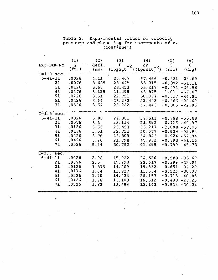
163

Table 2. Experimental values of velocitypressure and phase lag for increments of z.

(continued)

(1) (2) (3) (4) (5) (6)Exp-Sta-No z defl. U -2 Ap o 0 0

(ft.) (mm) (fpsxlO ) (fpsxlO ) (rad) (deg)T= 1.0 sec.6-41-11 .0026 4.11 26.407 67.466 -0.431 -24.6921 .0076 3. 685 23.475 53.315 -0.892 -51.11

31 .0126 3.68 23.453 53.217 -0.471 -26.9841' .0176 3.125 21.295 43.875 -1.01 -57.8751 .0226 3.51 22.751 50.077 -0.817 -46.8161 .0426 3.64 2 3.2 82 52.443 -0.466 -26.6971 .0526 3.64 23.282 52.443 -0.385 -22.06

T=1.5 sec.6-41-11 .0026 3. 88 24.381 57.513 -0.888 -50.88

21 .0076 3.6 23.114 51.692 -0.715 -40.9731 .0126 3.68 23.453 53.217 -1.008 -5 7.75

• 41 .0176 3.51 22.751 50.077 -0.924 -52.9451 .0226 3.76 23.809 54.843 -0.924 -52.9461 .0426 3.26 21.798 45.972 -0.893 -51.1671 .0526 5.64 30.752 • -91.495 -0.799 -45.78

T=2.0 sec.6-41-11 .0026 2.08 15.922 24.526 -0.588 -33.69

21 .0076 2.0 15.290 22.617 -0.399 -22.8631 .0126 1. 875 14.209 19.532 -0.651 -37.2941 .0176 1.64 11.827 13.534 -0.525 -30.0851 .0226 1.90 14.435 20.157 -0.713 -40.8561 .0426 1.76 13.103 16,612 -0.493 -28.2571 .0526 1. 82 13.694 18.143 -0.524 -30.02

164

Table 2. Experimental values of velocitypressure and phase lag for increments of z.

(continued)

(1) (2) (3) (4) (5) (6)Ejp-Sta-No 2 defl. U Ap 0 0____________ (ft.)_____ (mm) (fpsxlO" ) (fpsxlO ) (rad) (deg)T= 1.0 sec.6-43--11 .0026 5.08 29.205 82.521 -0.994 -56.95

21 .0076 5.04 29.093 81.887 -0.548 -31.3931 .0126 4.4 27.259 71.891 -0.893 -51.1641 .0176 4.8 28.413 78.105 -0.893 -51.1651 .0226 4.6 27.839 74.983 -0.768 -44.00

T=1.5 sec.6-43--11 .0026 4. 44 27.376 72.507 -0.548 -31.39

21 .0076 • 4 . 4 27.259 71.891 -0.674 -38.61. 31 .0126 4.11 .26.408 67.466 -0.589 -33.7541 .0176 4.08 26.318 67.012 -0.58.9 -33.7551 .0226 3.8 23.994 55.701 -0.548 -31.39

T=2.0 sec.6-43--11 .0026 3.0 20.820 41.938 -0.788 -45.15

21 .0076 2.92 20.505 . .. 40.6 81 -0.813 -46.5831 .0126 2.8 20.011 38.744 -0.813 -46.5841 .0176 2.72 19.662 . 37.403 -0.072 4,1251 .0226 2.62. . 19.19 8 35.659 -0.744- -42.63

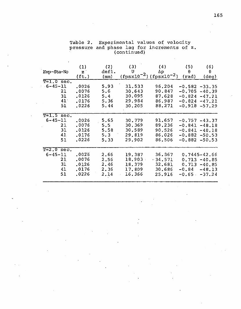
165

Table 2. Experimental values of velocitypressure and phase lag for increments of z.

(continued)'

(1) (2) (3) (4) (5) (6)Exp-Sta-No z defl U Ap 0 0

(ft.) (mm) (fpsxlO ) (fpsxlO- ) (rad) (deg)T=1.0 sec •

■6-45-11 .0026 5.93 31.533 96.204 -0.582 -33.3521 .0076 5.6 30.643 90.847 -0.705 -40.3931 .0126 5.4 30.095 87.628 -0.824 -47.2141 .0176 5. 36 29.984 86.987 -0.824 -47.2151 .0226 5.44 30.205 88.271 -0.918 -57.29

T=1.5 sec •

6-45-11 ,0026 5.65 30.779 91.657 -0.757 -43.3721 .0076 5.5 30.369 89.236 -0.841 -48.1831 .0126 5.58 30.589 90.526 -0.841 -48.1841 .0176 5.3 29.819 86.026 -0.882 -50.5351 .0226 5. 33 29.902 86.506 -0.882 -50.53

T=2.0 sec •

6-45-11 .0026 2.66 19.387 36.367 0.7445 -42.6621 .0076 2.56 18.903 - 34.571 0.713 -40.8531 .0126 2. 46 18.379 32.681 0. 713 -40.8541 .0176 2. 36 17.809 30.686 -0.84 -48.1351 .0226 2.14 16.366 25.916 -0.65 -37.24

166

Table 2. Experimental values of velocity pressure and phase lag for increments of z.

(1) (2) (3) (4) (5) (6)Exp-Sta-No z defl. U o AP _ o 0 0

(ft.) (mm) (fpsxlO )(fpsxlO ) (rad) (deg)T=1.0 sec.7-37-10 0.0026 7. 47 35.457 12.164 1.01 57.87

20 0.0076 8.0 36.719 13.045 • 0. 892 51.1130 0.0126 7.82 36.296 12.746 0.885 50.7140 0.0176 7.08 34.499 11.515 0.83 47.5550 0.0226 6.5 33.026 10.555 0.96 55.0060 0.0426 7.0 34.299 11.382 0.975 55.8670 0.0626 6.8 33.797 11.051 0.855 48.9880 0.0826 6.46 32.927 10.489 0.855 48.98

T=1.5 sec.7-37-10 0.0026 8. 88 38.717 14.503 0.5 38.65

20 0.0076 7.73 36.082 12.596 0.414 23.7230 0.0126 7.7 36.011 12.546 0.582 33.3540 0.0176 7.42 35.336 12.080 0.71 40.6850 0.0226 7.24 34.895 11.781 1.125 64.4660 0.0426 6.56 33.184 10.654 1.21 39.3370 0.0626 6. 35 32.641 10.308 1.29 73.9180 0.0826 6.8 33.797 11.051 0. 834 47.78

T=2.0 sec.7-37-10 '0.0026 5.6 30.643 9.085 0.45 25.78

20 0.0076 5.28 29.763 8.571 0.605 34.6630 0.0126 5.17 29.457 8.395 0.386 22.1240 0.0176 4.56 27.724 7.436 0.583 33.4050 0.0226 4.17 26.584 6. 837 0. 416 23.8360 0.0426 4.215 26.717 6.906 0.395 22.6370 0.0626 4.44 27.376 7.251 0.795 45.55

I

167

Table 2. Experimental values of velocitypressure and phase lag for increments of z.

(continued)

(1) (2) . (3) (4) (5) (6)Exp-Sta-No z defl. U Ap _ 0 0____________ (ft.) (mm) (fpsxlO" ) (fpsxlO" ) (rad) (deg)T=1.0 sec.7 - 39-10

20 30 40 50 60 70 80

0.00260.00760.01260.01760.02260.04260.06260.0826

8.757.547.667.57.47.98.17.32

38.429 35.627 35.915

- 35.529 35.2 87 36.485 36.953- 35.092

14.2.8912.28012.47912.21312.04712.87913.21111.914

0.595 0.665 0.99 0.68 0. 88 0.99 • 0.895 0.99

34.0938.1056.72 38.96 50.4256.72 51.2 856.72

T=1.S sec.7 -39-10 0.0026 10.2 41.481 16.647 .0.725 41.54

20 0.0076 9.68 40.425 15.811 0.932 53.3930 0.0126 9.1 39.197 14.865 0.91 52.1440 0.0176 8. 8 38.541- 14.371 0. 85 48.7050 0.0226 8.5 37.869 13.875 0. 81 46.4160 0.0426 8.7 38.319 • -14.206 0. 81 46.4170 0.0526 8.54 37.960 13.941 0.935 53.5780 0.0726 8.4 37.643 13.709 0.935 53.57

T=2.0 sec.7 -39-10 0.0026 6.1 31.985 9.898 0.855 48.98

20 0.0076 5.8 31.185 9.409 0. 855 48.9830 0.0126 5.6 30.643 9.085 0.795 45.5540 0.0176 5.6 30.643 9.085 0. 763 43.7250 0.0226 5.6 30.643 9.085 0.763 43. 7260 0.0426 5.3 29.819 8.603 . 0.763 43.7570 0.0526 5.6 30.643 9.085 0.855 48.9880 0.0726 5.6 30.643 9.085 1.11 63.59

168

Table 2. Experimental values of velocitypressure and phase lag for increments of z.

(continued)

Exp-Sta-No(1)z

(ft.)(2)

defl.(mm)

(3) (4)U -2 Ap -2 (fpsxlO ) (fpsxlO )

(5)0

(rad)(6)0

(deg)T=1.0 sec. 7 - 41-10 0.0026 12. 85 46.187 20.639 0.675 38.6 420 0.0076 10. 8 42.645 17.595 1.11 63.59

30 0.0126 10.8 42.645 17.595 0.905 51. 8540 0.0176 10. 7 42.455 17.438 1.73 99.1250 0.0226 10. 7 42.455 17.438 1.14 65. 3260 0.0426 9.5 40.049 15.519 1.19 68.18

T=1.5 sec.7 - 41-10 0.0026 14.1 48.017 22.307 0.182 10. 43

20 0.0076 13. 32 46.904 21.285 0.182 10. 4330 0.0126 ' 12.32 45.335 19.885 0.331 18.9640 0.0176 11.62 44.142 18.852 0.372 21. 3150 0.0226 12.0 44;800 19.418 0.456 26.1260 0.0426 10.5 42.069 17.12 4 0.456 26.12

T=2.0 sec.7 -41-10 0.0026 6. 86 33.948 ‘ 11.150 0.355 20.34

2.0 0.0076 6. 7 33.543 10.885 0.858 49.1630 0.0126 6.2 32.245 10.061 0. 858 49.1640 0.0176 6.4 32.771 10.390 0.64 36.6 750 0.0226 6.4 32.771 10.390 0.573 32. 8360 0.0426 5.5 30.369. 8.923 ,0.762 43.66

169

Table 2. Experimental values of velocitypressure and phase lag for increments of z .

(continued)

(1) (2) (3) (4) (5) (6)Exp-Sta-No z defl. u Ap o 0 0

(ft.) (mm) (fpsxlO ) (fpsxlO ) (rad) (deg)T=l.0 sec •

7 - 43-10 0.0026 17. 8 51.968 26.129' -0.035 - 2.0020 0.0076 15.1 49.301 23.516 -0.115 - 6.5930 0.0126 13.4 47.023 21.393 0.02 1.1440 0.0176 13.0 46.419 . 20.848 -0.19 -10.8950 0 .0226 13.25 46.799 21.190 0.065 3. 7260 0.0426 11.42 . 43.787 18.549 0. 37 21.19

T=1.5 sec •

7 - 43-10 0.0026 15. 8 50.105 24.289 0.04 2.2920 0.0076 18. 83 52.679 26.849 -0.146 - 8.36

' 30 0.0126 15.2 . 49.401 23.603 -0.255 -14.6140 0.0176 14.4 48.419 22.682 0.04 2.2950 0.022.6 14.65 48. 743' 22.987 -0.045 - 2.5860 0.0426 14.1 48.017 22.307 -0.045 - 2.58

T=2.0 sec - -

7 - 43-10 0.0026 8.4 37.643 13.709 0.198 11.3420 0.0076 9.25 39.519 15.111 . 0.. 511 29.2930 0.0126 9.2 39.413 15.029 0.511 29.2940 0.0176 9.0 38.979 14.700 0. 386 22.1150 0.0226' 9.0 38.9 79 14.700 0. 383 21.9460 0.0426 7.5 35.529 12.213 0.29 +16.6170 0.0626 7. 35 35.165 11.964 0.29 +16.61

170

Table 2. Experimental values of velocitypressure and phase lag for increments of z.

(continued)

(1) (2) (3) (4) (5) (6)Exp-Sta-No z defl. U 0 0

(ft.) (mm) (fpsxlO )(fpsxlO ) (rad) (deg)T— 1.0 sec.7 -45-10 0.0026 27.1 • 52.229 26.392 -0.396 -22.69

20 0.0076 22.4 53.827 28.032 -0.283 -16.2130 0.0126 21.6 53.747 27.949 -0.345 -19.7740 0.0176 21.9 53.789 27.992 -0.327 -18.7350 0.0226 20.0 53.280 27.465 -0.237 -13.5860 0.0426 20.0 .53.280 27.465 -0.15 - 8.59

T=1.5 sec.7 - 45-10 0.0026 22.4 53.827 28.032 -0.312 -17.88

20 0.0076. 20.4 53.435 27.625 -0.0 75 - 4.2930 0.0126 19.4 52.999 27.176 -0.015 - . 8640 0.0176 22.7 53.831 38.036 -0.075 - 4.2950 0.0226 18.72 52.611 26.779 -0.05 - 2.8660 0.0426 18. 70 • 52.598 26.767 0.115 + 6.59

T=2.0 sec.7 - 45-10 0.0026 10. 35 41.777 ' “16.886 -0.101 -5.79

20 0.0076 10. 38 41.836 16.934 -0.147 - 8.4230 0.0126 9.51 40.071 15.535 0.01 + .5740 0.0176 9.8 40.673 16.005 -0.065 - 3.7250 0.0226 9.2 39.413 15.02 8 -0.085 - 4.8760 0.0426 9.2 39.413 15.02 8 0.023 + 1.32

171

Table 2. Experimental values of velocitypressure and phase lag for increments of z .

(continued)

(1) (2) (3) (4) (5) (6)Exp-Sta-No z defl U Ap 0 0

(ft.)■ (mm) (fpsxlO ) (fpsxlO ) (rad) (deg)'T=1.0 sec • •7 - 37-11 0.0026 9.0 38.979 14.700 -0.62 -35152

' 21 0.0076 7.2 34.79 7 11.745 -1.024 -58.6731 0.0126 8.84 38.629 14.436 -7.27 -41.65'41 0.0176 8. 38 -37.59 0 13.676 -0.686 -39.3051 0.0226 8.2 37.185 13.378 -0.584 -33.4661 0.0426 7.72 • 36.058 12.579 -0.572 -32.77.

T=1.5 sec •

7 - 37-11 0.0026 9.8 40.673 16.005 -0.673 -38.5621 0.0076 8.8 38.541 14.371 -0.673 -38.5631 0.0126 9.8 40.673 16.005 -0.749 -42.9141 0.0176 10.42 41.914 16.997 -0.589 -33.7551 • 0.0226 9. 84 .. 40.755 .. 16.069 -0.673 -38.5661 0.0426 10.0 41.079 16.327 -0.631 -36.15

T=2.0 sec • -

7 -37-11 0.0026 7.64 35.86 7 12.446 -0.745 -42.6821 0.0076 6.56 33.184 10.645 -0.619 -35.4631 0.0126 6.7 33.543 10.885 .-0.87 -49.8441 0.0176 6.3 32.511 . 10.226 -0.713 -40-. 8551 0'i, 0226 6.48 32.9 78 10.522 -0.745 -42.6861 0.0426 6.5 33.029 10.555 -0.745 -42.68

172

Table 2. Experimental values of velocitypressure and phase lag for increments of z.

(continued)

(1) (2) (3) (4) (5) (6)ixp - Sta-No 2 defl u Ap ~ 0 0

(ft.) (mm) (fpsxlO ) (fpsxlO ) (rad) (deg)-1.0 sec • .

7 -39-11 0.0026 11.44 43.823 18.580 -0.344 -19.7121 0.0076 10.16 41.401 16.583 -0.344 -19.7131 0.0126 8.8 38.541 14.311 -0.475 -2 7.214i 0.0176 9.35 39.733 15.274 -0.535 -30.6551 0.0226 9.52 40.092 15.551 -0.234 -13.4161 0.0426 11. 47 43.876 18.626 0.13 7.45

T=.l. 5 sec.7 - 39-11 0.0026 11.1 43.205 18.060 -0.601 -34.43

21 0.0076 10.7 42.455 17.438 -0.807 -46.2331 0.0126 10.42 41.914 16.997 -0.842 -48.2441 0.0176 9. 88 40.836 16.134 -0.842 -48.2451 0.0226 10.22 41.'520 16.679 -0.842 -48.2461 0.0426 10.05 41.181 16.407 -0.722 -41.36

T=2.0 sec.7 - 39-11 0.0026 4.86 28.584 7.905 -0.467 -26.76

21 0.0076 5.4 30.095 8.76 3 -0.405 -23.2031 0.0126 5.6 30.643 9.085 -0.368 -21.08• 41 0.0176 5.6 30.643 9.085 -0.494 -28.3151 0.0226 5.68 30.860 9.214 -0.556 -31.8661 0.0426 5.6 30.643 9.085 -0.588 -33.6971 0.0626 5.7 30.915 9.2 4.7 -0.619 -35.46

173

Table 2. Experimental values, of velocitypressure and phase lag for increments of z.

(continued)

(1) (2) (3) (4) (5) (6)Exp-Sta-No z defl. U Ap 0 0____________ (ft.)_____ (mm) (fpsxlQ1" ) (fpsxlO ) (rad) (deg)T=1.0 sec.7 -41-11 0.0026 13.7 47.459 21.791 -0.65 -37.24

21 0.0076 12.5 45.629 20.144 -0.59 -33.8031 0.0126 15.9 ' 50.213 24.394 -0.344 -19.7141 0.0176 15.6 49.883 24.075 -0.588 -33.6951 0.0226 16. 3 50.631 ■ 24.802 -0.315 -18.0561 0.0426 16.2 50.529 24.702 -0.235 -13.4671 0.0626 15.4 49.655 23.855 -0.235 -13.46

T=1.5 sec.7 - 41-11 0.0026 10.7 42.455 17.438 -0.753 -43.14

21 0.0076 10. 4 41.875 16.965 -0.845 -48.1131 0.0126 10.6 42.263 17.282 -0.75 -42.9741 0.0176 11.0 43.019 17.906 -0.64 -36.6751 0.0226 10.3 41.679 16.807 -0.557 -31.9161 0.0426 10.5 42.069 17.124 -0.393 -22.52

■ 71 0.0626 9.8 40.673 • -16.005 -0.547 -31.34T=2.0 sec.7 - 41-11 0.0026 7. 3 35.043 11.881 -0.304 -17.42

21 0.0076 6.9 34.049 11.217 -0.305 -17.4731 0.0126 6.8 33.797 11.051 -0.37 -21.1941 0.0176 7.1 34.549 11.548 -0.18 -10.3151 0.0226 6.9 34.049 11.216 -0.305 -17.47561 0.0426 7.0 .34.999 11.382 -0.65 -37.24

174

Table 2. Experimental values of velocitypressure and phase lag for increments of z.

(continued)

(1) (2) (3) (4) (5) (6)Exp-Sta- No z defl. U Ap e 0

(ft.) (mm) (fpsxlO ) (fpsxlO^) (rad) (deg)T=1.0 sec.7 -43-11 0.0026 18. 3 52.335 26.499 -0.649 -37.1821 0.0076 17.9 52.045 26.207 -0.527 -30.19

31 0.0126 16.9 51.209 25.371 -0.466 -26.6941 0.0176 20. 8 53.565 27.759 -0.405 -23.2051 0.0226 18. 4 52.403 26.568 -0.345 -19.7761 0.0426 18.2 52.265 26.428 -0.405 -23.2071 0.0576 19.00 52.780 26.952 -0.172 -9.8581 0.0726 21.6 53.747 27.949 -0.466 -26.69

T--1.5 sec.7 -43-11 0.0026 12. 8 46.109 20.569 -0.673 -38.56

21 0.0076 11. 8 44.457 19.122 -0.613 -35.1231 0.0126 12.95 46.343 20.778 -0.757 -43.3741 0.0176 12.1 44.969 19.565 -0.631 -36.1551 0.0226 13.2 46.724 21.122. -0.547 -31.3461 0.0426 13.2 46.724 = -21.122 -0.506 -28.99

T=2.0 sec.7 - 43-11 0.0026 8.6 38.095 14.041 -0.524 -30.02

21 0.0076 10.95 42.927 17.82 8 -0.43 -24.6431 0.0126 10.6 42.263 17.282 -0.368 -21.0841 0.0176 10.53 42.128 17.171 -0.242 -13.8651 0.0226 11.05 43.123 17.983 -0.242 -13.8661 0.0426 12.4 45.461 20.000 -0.242 -13.86

175

Table 2. Experimental values of velocitypressure and phase lag for increments of z.

(continued)

(1) (2) (3) (4) (5) (6)Exp-Sta-No z defl. U AP 0 0

(ft.) (mm) (fpsxlO )(fpsxlO ) (rad) (deg)T=1.0 sec.7-45-11 0.0026 21.65 53.755 27.958 -0.10 - 5.73

21 0.0076 22.0 53.800 28.004 -0.344 -19.7131 0.0126 23.5 53.769 27.974 -0.344 -19.7141 0.0176 23.4 53.7 83 27.986 -0.344 -19.7151 0.0226 26.9 52.369 26.534 -0.405 -23.2061 0.0426 23.8 53.721 27..921 -0.588 -33.68

T=1.5 sec.7-45-11 0.0026 12.6 45.791 20.287 -0.464 -26.58

21 0.0076 13.1 46.573 20.985 -0.214 -12.2631 0.0126 13.65 47.387 21.726 -0.295 -16.9041 0.0176 13. 8 47.601 21.922 -0.214 -12.2651 0.0226 13.5 47.170 21.527 -0.254 -14.5561 0.0426 15.46 49.724 23.921 -0.124 - 7.10

T=2.0 sec. - ■

7-45-11 0.0026 . 9.95 40.979 16.247 -0.462 -26.4721 0.0076 10.5 42.069 17.127 -0.368 -21.0831 0.0126 12. 3 45.303 19.856 -0.556 -31.8641 0.0176 11.55 44.019 18.746 -0.524 -30.0251 0.0226 12.1 44.969 19.565 -0.368 -21.0861 0.0426 13.3 46.875 21.258 -0.405 -23.20

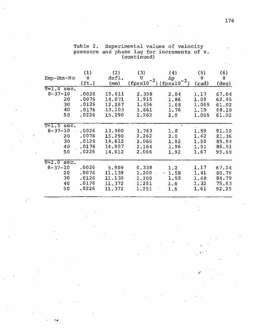
176

Table 2. Experimental values of velocitypressure and phase lag for increments of z.

(continued)

(1) (2) (3) (4) (5) (6)Exp-Sta-No z defl. U Ap o 0 0

(ft.) (mm) (fpsxlO ) (fpsxlO ) (rad) (deg)T=1.0 sec.8-37-10 .0026 15.611 2. 358 2.04 1.17 67.04

20 .0076 14.071 1.915 1.86 1.09 62. 4530 .0126 12.267 1.456 1.68 1.065 61.0240 .0176 13.103 1.661 1.76 1.19 68.1850 .0226 15.290 2.262 2.0 1.065 61. 02

T=1.5 sec. «8-37-10 .0026 13.500 1.763 1.8 1.59 91.10

20 .0076 15.290 2.262 2.0 1.42 81. 3630 .0126 14.612 2.066 1.92 1.50 85.9440 .0176 14.957 2.164 1.96 1.51 86.5150 .0226 14.612 2.066 1.92 1.67 95.68

T=2.0 sec.8-37-10 .0026 5.909 0. 338 1.2 1.17 67.04

20 .0076 11.139 1.200 -- 1.58 1.41 80.7930 .0126 11.139 1.200 1.58 1.48 84.7940 .0176 11.372 1V 2 51 1.6 1.32 75.6350 .0226 11.372 1.251 1.6 1.61 92.25

177

Table 2. Experimental values of velocitypressure and phase lag for increments of z.

(continued) ■

(1) (2) (3) (4) (5) (6):xp-Sta-No z defl u Ap 0 0

(ft.) (mm) (fpsxlO” ) (fpsxlO""^) (rad) (deg)'=1.0 sec •

8-39-10 .0026 2. 84 20.179 3.939 0.94 53. 8620 .0076 2.8 20.011 3. 874 1.065 61.0230 .0126 2.68 19.480 3.671 1.13 64. 7440 .0176 2.68 19.480 3.671 1.25 71.6250 .0226 2.71 19.617 3.723 1.28 73.3460 .0426 2.48 18.487 3. 307 1.07 61.3170 .0526 2.44 18.269. 3.229 1.255 71.91

'=1.5 sec »

8-39-10 .0026 3.2 21.575 4.503 0.96 55.0020 .0076 3.08 21.126 4. 318 1.21. 69.3330 .0126 3.04 20.974 4.256 1.21 69. 3340 .0176 3.0 20.820 4.194 1.21 69 . 3350 .0226 2. 32 17.567 2.986 1.19 68.1860 .0426 2.3 17.443 2.944 1.27 72. 7670 .0526 2.6 19.101 . _3.530 1.045 59. 87

8-39-10 .0026 1.62 11.602 1. 302 1. 36 77.9220 .0076 1.62 11.602 1. 302 1.32 75.6330 .0126 1.68 12.267 1. 455 1.51 86.5240 .0176 1. 66 12.049 1. 405 1.21 69.3350 .0226 1.76 13.103 1.661 1. 39 79.64

178

Table 2. Experimental values of velocitypressure and phase lag for increments of z.

(continued)

(1) (2) (3) (4) (5) (6)Ejp-Sta-No z defl. U 0 Ap 0 0____________(ft.)______(mm) (fpsxlO- ) (fpsxlO ) (rad) (deg)T= 1.0 sec. 8-41-10

20 30 40 50 60

.0026

.0076

.0126

.0176

.0226

.0426

3.4 3. 45 3.56 3. 323.243.24 :

22.324 22.516 22.951 22.02221.72421.724

4. 821 4.905 5.096 4.692 .4.5664.566

1.32 1. 321.191.251.251.19

75.6 3 75.63 68.1871.6271.62 68.18

T=1.5 sec.8-41-10 .0026 3.48 22.633' 4.956 1.335 76.49

20 .0076 • 3.6 2 3.11-4 5.169 0.96- 55.0030 .0126 3.52 22.790 5.025 1.21 69.3340 .0176 ' 3.4 ■ 22.324 4.821 1.255 71.9150 .0226 3.52 22.790 5.025 1.17 67.0460 .0426 3. 34 22.097 4.724 1.29 73.9170 .0526 3.08 21.126 4. 318 1.085 62.16

T=2.0 sec.8-41-10 .0026 1. 82 13.694 1.814 1.61 92.95

20 .0076 1.94' 14.786 2:115 ' 1.26 72.19.30 .0126 1.77 13.204 1.687 1.37 78.6940 .0176 1. 88 14.254 1.966 1.29 73.9150 .02-2 6 1.77 13.204 1.687 1.64 93.96

179

Table 2. Experimental values of velocitypressure and phase lag for increments of z.

(continued)

(1) (2) (3) (4) (5) (6)Ixp-Sta-No z def 1. U Ap 0 e 0

(ft.) (mm) (fpsxlO-^)(fpsxlO ) (rad) (deg)'=1.0 sec.8-43-10 .0026 4.92 28.754 7.999 0. 82 46.98

20 .0076 4. 84 28.527 7. 873 0.5 28.6430 .0126 4.48 27.492 7.312 0.44 25.2140 .0176 3.92 24.584 5. 847 1.0 57.2950 .0226 4.13 26.466 6.777 0. 815 46.6960 .0426 3.8 23.994 5.570 0.565 32 . 3770 .0526 4.16 26.555 6. 822 0.72 41.25

'=1.5 sec. 8-43-10

20 30 40

.0026

.0076

.0126

.0176

4.24.484.324.4

26.673 27.492 27.025 27.259

6. 8837. 312 7.066 7.189

0.71 0. 46 0.71 0.625

40.68 26.3640.68 35.81

'=2.0 sec.8-43-10 .0026 1.64 11.. 82 7 -1.353 1.54 88.23

20 . 0076 1.72 12.692 1.559 1.45 83.0830 .0126 1.76 13.103 1.661 1. 39 79.6440 .0176 1.64 11.827 1. 353 1.26 72.1950 .0226 1.76 13.103 1.661 1. 39 79.64

180

Table 2. Experimental values of velocitypressure

(1)Exp-Sta-No z(ft.)

and phase lag for (continued)

(2) (3) defl. U (mm) (fpsxlO )

increments

(4)Ap _2 (fpsxlO )

of z.

(5)6

(rad)(6)0

(deg)T=1.0 sec.8-45 -10 .0026 6.53 33.107 10.605 0. 315 18.05

20 .0076 5.7 30.915 9.247 0.69 39.5330 .0126 5.98 31.667 9.702 0.565 32.3740 .0176 5.66 30.806 . 9.182 0.63 36.09.50 .0226 5.52 30.424 8.956 0. 81 46.4160 .0426 4. 76 28;298 7.748 1.13 64. 7470 .0526 4. 82 28.469 7.842 0. 82 46. 98'

T=1.5 sec.8-45'-10 .0026 5.2 29.541 8.443 0.039 "2.23

20 .0076 5.12 29.317 8.316 0.08 4.5830 .0126 4.95 28.839 8.046 0.08 : 4.5840 .0176 4.75 28.269 7.732 0.29 16.6150' .0226 4.76 28.298 7.747 0.29 16.6160 .0426 4.71 28.155 7.669 0.42 24.06

• 70 .0526 . 4.5 27.549 . - 7.343 0.50 28.65T=2 .0 sec.8-45--10 .0026 1. 88 14.254 1.966 1.45 83.08

20 .0076 1.96 14.957 2.164 1.075 61.5930 .0126 1.98 15.125 2.213 1.14 65.3240 .0176 2.0 15.290 2.262 1.14 65. 3250 .0226 2.0 15.290 2.262 1.14 65.3260 .0426 2.02 15.452 2.310 1. 33 76.2070 .0526 2.02 15.452 2. 310 1.08 61. 88

181

Table 2. Experimental values of velocitypressure and phase lag for increments of z.

(continued)

Exp-Sta-No(1)z

(ft.)(2)

defl. (mm)

(3) (4)U -2 AP -(fpsxlO ) (fpsxlO

(5) (6)0 0

2) (rad) (deg)T-1.0 sec.8-37 -11 .0026 2.96 20.664 4.131 -1.131 -64.80

21 .0076 2.96 20.664 4.131 -1.163 -66.6331 .0126 2.96 20.664 4.131 -1.257 -72.0241 .0176 2.96 20.664 4.131 -1.32 -75.6351 .0226 2.96 20.664 4.131 -1.32 -75.6361 .0426 2. 84 20.179 3.939 -1.32 -75.63

T=l. 5 sec.8-37--11 .0026 3.4 22.324 4. 822 -0.966 -55.3521 .0076 3.24 21.724 4.566 -0.841 -48.18

31 .0126 3.16 21.426 4.441 -0.966 -55.3541 .0176 3.12 21.276 4.379 -0.841 -48.1851 .0226 3.12 21.276 4. 379 -0.966 -55.3561 .0426 3.08 21.126 4. 318 -1.008 -57.75

T=2.0 sec. -

8-37--11 .0026 2.32 17.567 2.986 -0.87 -49.8521 .0076 2.24 17.057 2. 815 -0,87 -49.8531 .0126 2.2 16.788 2. 72 7 -0.87 -49.8541 .0176 2.4 17.057 2. 815 -0.807 -46.2451 .0226 2.12 16 .221 2.545 -0.745 -42.6861 .0426 2.16 16.509 2. 637 -0.745 -42.6871 .0526 2. 36 17.809 3.067 -0.776 -44.46

182

Table 2. Experimental values of velocitypressure and phase lag for increments of z.

(continued)

(1) (2) (3) (4) (5) (6)Exp-Sta-No z defl. u Ap 0 0 0

(ft.) (mm) (fpsxlO" ) (fpsxlO- ) (rad) (deg)T= 1.0 sec.8-39-11 .0026 3.24 21.724 4.566 -1.132 -64.8621 .0076 2. 77 19.882 3. 825 -0.943 -5 4.0 3

31 .0126 2.695 19.549 3.697 -1.068 -61.1941 .0176 2.8 20.011 3. 874 -0.880 -50.4251 . 0226 2.8 20.011 3. 874 -0.944 -54.09

T=1.5 sec.8-39-11 .0026 3.48 22.633 4.956 -0.589 -33.75

21 .0076 3. 36 22.172 4.756 -0.799 -45.7831 .0126 3.24 21.724 4.566 -1.05 -60.1641 .0176 3.24 21.724 4.566 -1.05- -60.1651 .0226 3. 36 22.172 4. 756 -0.841 -48.1861 .0426 3. 39 22.286 4. 8Q5 -0.925 -52.99

T=2.0 sec.8-39-11 .0026 2.28 17.317 -2.901 -0. 87 -49.8521 .0076 2.28 17.317 2.901 -0.901 -51.62

31 .0126 2.08 15.922 2. 452 -0.839 -48.0741 .0176 2.2 16.788 2. 727 -1.027 -58.8451 .0226 2.12 16.221 2.546 -0.901 -51.6261 .0426 2.12 16.221 2.546 -0.901 -51.62

183

Table 2. Experimental values of velocitypressure and phase lag for increments of z.

(continued)

(1) (2) (3) (4) (5) (6)Exp-St a -No z defl. U Ap 0 0 _________ (ft.)___(mm) (fpsxlO" ) (fpsxlO ) (rad) (deg)T=1.0 sec. 8-41-11

21 31 41 51

.0026

.0076

.0126

.0176

.0226

4.024.194.123.963.68

26.139 26.643 26.436 24.793 23.453

6.611 6.868 6.762 5.947 5. 322

-1.226 -70.24 -1.163 -66.63 -1.132 -64.86 -1.006 -57.64 -0. 818 -4.6. 87

4

T=1.5 sec.8-41-11 .0026 3.6 23.114 5.169 -1.05 -60.16

21 .0076 3.64 23.282 5.244 -1.05 -60.1631 .0126 3.64 23.2 82 •5.244 -1.008 -57.7541 .0176 3.6 23.114 5.169 • -0.988 -56.6151 .0226 3. 42 22.400 4.855 -0.674 -38.62

T - 2 .0 sec.8-41-11 .0026 2.04 15.611 2.358 -0.651 -37.29

21 .0076 1.96 14.957 . -2.164 -0.901 -51.6231 .0126 1.96 14.957 2.164 -0.901 -51.6241 .0176 ' 2.0 15.290 2.262 -0-. 87 -•49.8 451 .0226 2.12 16.221 2.546 -0.776 -44.46

184

Table 2. Experimental values of velocitypressure and phase lag for increments of z.

(continued)

Exp-Sta-No (1) z • (ft.)

(2)defl.(mm)

(3) (4)u -2 AP -2 (fpsxlO ) (fpsxlO )

(5)0

(rad)(6)0

(deg)T=1.0 sec. 8-43-11 .0026 5.0 28.979 . 8.125 -1.10 -63.02

21 .0076 5.4 30.095 8.763 -1.069 -61.2531 .0126 4.95 28.839 8.046 -1.132 -64.8641 .0176 5.0 8 29.205 8.252 -1.006 -57.6451 .0226 4.8 28.413 7. 810 -0.818 -46.87

T=1.5 sec. 8-43-11 .0026 5. 01 29.008 8.141 -0.757 -43.37

21 .0076 5.04 29.093 8.189 -0.799 -45.7831 .0126 4.92 28.754 7.999 -0.841 -48.1841 .0176 4. 86 28.584 7.905 -0.799 -45.7851 . 0226 4.76 28.298 7.747 -0.799 -45.7861 .0426 4.77 28.327 7.763 -0.799 -45.78

T=2.0 sec. 8-43-11 .0026 2.8 20.011 : 3.874 -0. 87 49.84

21 .0076 2. 84 20.079 3.939 -0.839 -48.0731 .0126 2.8 20.011 3. 874 -0.839 -48.0741 .0176 2.64 19.294 3.601 -0.839 -48.0751 .0226 2.64 19.294 3.601 -0. 87 -49.8461 .0426 2.68 19.480 3.671 -0.744 -42.6 3

185

Table 2. Experimental values of velocitypressure and phase lag for increments of z.

(continued)

(1) (2) (3) (4) (5) (6)Exp-Sta-No z defl. U -2 Ap 2 6 0

(ft.) (mm) (fpsxlO ) (fpsxlO *) (rad) (deg)T= 1.0 sec •

8-45-11 .0026 36 .907 13.178 8.08 -0.992 -56.8421 .0076 37.299 13.461 8.25 -1.069 -61.2531 .0126 37.138 13.344 8.18 -1.132 -64.8641 .0176 36.058 12.579 7. 72 -1.006 -57.6451 .0226 35.602 12.263 7.53 -1.132 -64.8661 .0426 34.299 11.382 7.00 -1.19 -6 8.18

T= 1.5 sec • ■8-45-11 .0026 35.092 11.914 7.32 -0.883 -50.59

21 .0076 36.675 12.313 7.56 -0.841 -48.1831 .0126 34.475 11.498 7; 0 7 -0.5 47 -31.3441 .0176 34.598 11.582 7.12 -0.799 -45.7851 .0226 34.598 11.582 7.12 -0.589 -33.7561 .0426 33.398 11.117 6. 84 -0.631 -36.15

T=2.0 sec • -

8-45-11 .0026 23.809 ■5. 484 3. 76 -0.713 -40.8521 .0076 26.554 6.822 4.16 -0.493 -2 8.2531 .0126 25.009 6.052 4.0 -0.493 -28.2541 .0176 25.009 6.052 4.0 -0.65 -37.2451 .0226 25.009 6.052 4.0 -0.839 -48.0761 .0426 24.584 5.847 3.92 -0.87 -49.84

t

N

Table 3. Averaged experimental wave ;— and computed and experimental' boundary layercharacteristics. Smooth boundary. Large amplitude waves (stroke = 1.125 ft.)

(1) (2) (3) (4) (5) (6) (7) (8) (9> (lo) (XlT" fl2T (137 : (ITT (15)Test ^ Ho H d/L H/Hq 0 6l ?-RS. ^L(c) 5L(c) 5L(t) ^L(t)No. (sec) (ft) (ft) (f p sxl0~2) (ftxlO'"3) (ftxlO-s) (ftxlO's) (ftxlO-3) (ftxlO-1)(ftxlO"*)5-37 1.0 .480 .432 .276 ;432 .317 ;9oo 41.762 1.79 1.27 52 11.9 ‘ 8.4 6.9 4.91.5 .284 .258 .165 .114 .176 .908 40.150 2.18 1.54 61 14.5 * 10.2 7.5 5.32.0 .200 .169 .108 .042 .123 845 31.076 2.54 ' 1.79 55 14.5 10.2 • 12.5 8.85-39 1.0 .480 .430 .303 .430 .287 .896 45.676 1.79 12.7 57 16.7 11.8 7.3 5.21.5 .284 .267 .188 .119 .159 .94 47.532 2.18 1.54 72 12.6 . 8.9 8.2 5.82.0 .200 .181 .133 .045 .112 .905 37.229 2.54 1.79 66 • • - - 14.1 9.95-41 1.0 .480 .420 .336 .420 .253 .875 56.071 1.79 - il.27 70 15.8’ 11.2 8.0 5.6-1.5 .284 .265 .212 .118 .140 .933 55.468 2.18 1.54 84 8.7 • 6.1 8.7 6.12.0 .200 .203 .162 .051 .098 :1.015 48.473 2.54 1.79 . 86 12.6 8.9 14.1 9.95-43 1.0 .480 .417 .385 .417 .219 .869 70.548 1.79 1.27 • 88 22.6 15.9 ' '6.2 4.41.5 .284 .268 .247 .119 .121 .944 66.792 2.18 1.54 101 12.6 • 8.9 9.0 6.42.0 .200 .185 .171 .046 .085 .925 51.525 2.54 1.79 91 7.0 ' 4.9 . 8.9 6.35-45 1.0 .480 .423 .461 .423 .186 . 8S1 91.538 1.79 1.27 115 8.1 5.7 10.6 7.51.5 .284 .265 .289 .118 .103 - .933 79.622 2.18 1.54 121 ■ • 15.0 10.6 9.5 6.72.0 .200 .196 .213 .049 .072 .980 65.472 2.54 1.79' 116 8.7 6.1 5.9 4.2

186

\

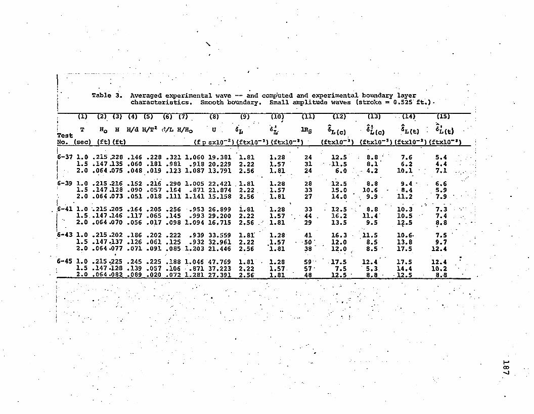
Table 3. Averaged experimental wave — and computed and experimental boundary layercharacteristics. Smooth boundary. Small amplitude waves (stroke = 0.525 ft.)-

r HI (2) (3) (4) (5) (6) (7) (8) (9) (To) (II) fl2) fl3) H T j (IITLest T H° “ H/d H/Ti d/L H/H° 0 K «L(C) «L(c) ?Mt) • 6L(t)No. (sec) (ft)(ft) (f p sxlO-2)(ftxlO-*)(ftxlO-’) (ftxlO-3) (ftxlO“J)(ftxlO-3)<ftxl0_3)i‘6-37 1.0 .215 .228 .146 .228 .321 1.060 19.381 1.81 1.28 24 12.5 8.8 • 7.6 5.4!I 1.5 .147 .135 .060 .181 .981 .918 20.229 2.22 1.57 31 11.5 8.1' 6.2 4.411I 2.0 .064 .075 .048 .019 .123 1.087 13.791 2.56 1.81 24 6.0 4.2 10.1 7.1 .6-39 1.0 .215 .216 .152 .216 .290 1.005 22.421 . 1.81 1.28 28 12.5 8.8 9.4 • 6.61.5 .147 .128 .090 .057 .164 .871 21.874 2.22 1.57 33 15.0 10.6 - 8.4 5.9:• 2.0 .064 .073 .051 .018 .111 1.141 15.158 2.56 1.81 27 14.0 ‘ 9.9 11.2 7.9

. 6-41 1.0 .215 .205 .164 .205 .256 .953 26.899 i.81 1.28 33 12.5 8.8 10.3 7.3 -j 1.5. .147 .146 .117 .065 .145 .993 29.200 2.22 1.57 44 16.2 11.4 10.5 7.4| 2.0 .064 .070 .056 .017 .098 1.094 16.715 2.56 . 1.81 29 13.5 9.5 12.5\ 8.86-43 1.0 .215 .202 .186 .202 .222 .939 33.559 1.81' 1.28 41 16.3 11.5 10.6- 7.51.5 .147.137 .126 .061 .125 .932 32.961 2.22 .1.57 50' 12.0 8.5 13.8 9.72.0 .064 .077 .071 .091 .085 1.203 21.446 2.56 1.81 38 ' 12.0 8.5 17.5 12.46-45 1.0 .215 .225 .245 .225 .188 1.046 47.769 1.81 1.28 59 - 17.5 12.4' 17.5 12.4 r1.5 .147.128 .139 .057 .106 ■ .871 37.223 2.22 1.57 57 7.5 5.3 14.4 10.22.0 .064 .082 .089 .020 .072 1.281 27.391 2.56 1.81 48 12.5 ' 8.8 12.5 8.8

187

Filmed as received

without page(s) 188

UNIVERSITY MICROFILMS.

Table 3. Averaged exp erim en ta l wave— and computed and exp er im en ta l boundary la y e r c h a r a c t e r i s t i c s .

Rough boundary. Large am plitude waves ( s t r o k e = l .125 f t . )

T est No. (1)T

( s e c . )

(2)Ho( f t )

(3)H

(f t )

(4)H/d

(5)H/T

(6)d/L

(7)h /Hq

(8)U -2' (fpsxlO )

(9)IRr

(10)E R(c )exp

(11)^ ( t )exp7-37 1.0 .441 .429 .274 .429 .317 .973 37.325 1369 1301 14301.5 .260 .265 .169 .118 .176 1.019 41.239 1513 1420 14912.0 .179 .169 .108 .042 .123 .944 31.076 1140 1124 1316

7-39 1.0 .441 .416 .29 3 .416 .287 .943 44.189 1621 1410 15741.5 .260 .269 .189 .119 .159 1.035 47.888 1757 1522 15522.0 .179 .183 .129 .046 .112 1.022 37.640 1381 1173 1027

7-41 1.0 .-441 .410 . 32 8 .410 .253 .929 54.736 2008. 1695 17051.5 .260 .242 .194 .107 .140 .931 50.654 1858 1762 15252.0 .179 .182 .146 .045 .098 1.017 -43.558 1598 12 45 1259

7-43 1.0 .441 .413 .381 .413 .219 .936 68.871 2527 1907 18801.5 .260 .278 .257 .123 ' .121 1.069 69.294 2542 1838 16572.0 .179 1180 .166 .045 .085 1.005 50.554 1855 1381 1369

7-45 1.0 . 441 .412 .449 .412 .186 1.070 89.158 3271 1916 19 311.5 .260 .264 .288 .117 .10 3 1.015 79.321 2910 19 75 16452.0' <Z. .179 .177 .193 .044 .072 .989 59.378 2178 1533 1472

189

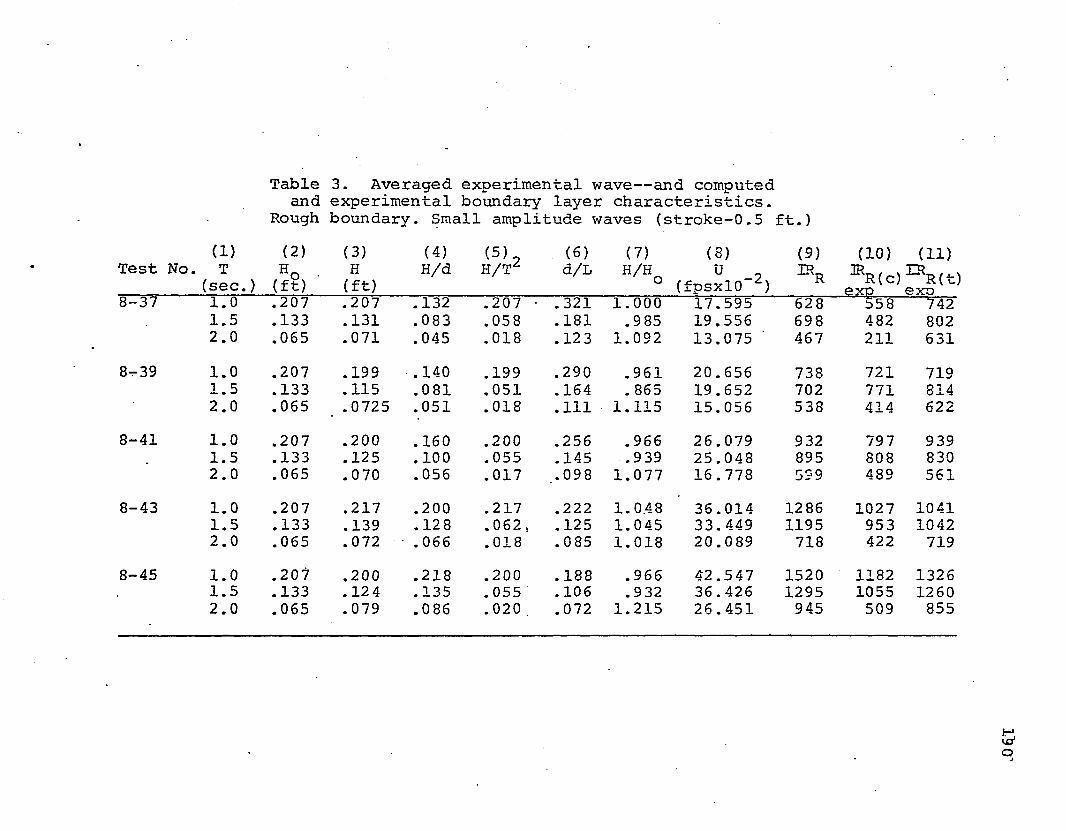
Table 3. Averaged experimental wave— and computed and experimental boundary layer characteristics.

Rough boundary. Small amplitude waves (stroke-0.5 ft.)(1) (2) (3) (4) (5) (6) (7) (8) (9) (10) (11)

Test No. T H^ H H/d H/T d/L H/H U „ 33L. 3R^,Test No. T (sec.) Ho • (ft)

H(ft)

H/d H/Tz d/L H/Ho U _2(fpsxlO z) ® R K R(c )exo ^ ( t )exo8-37 1.0 .207 .207 .132 .207 • .321 1.000 17.595 62 8 558 7421.5 .133 .131 .083 .058 .181 .9 85 19.556 698 482 8022.0 .065 .071 .045 .018 .123 1.092 13.075 ' 467 211 631

8-39 1.0 .207 .199 .140 .199 .290 .961 20.656 738 721 7191.5 .133 .115 .081 ,051 .164 . 865 19.652 702 771 8142.0 .065 .0725 .051 .018 .111 1.115 15.056 538 414 622

8-41 1.0 .207 .200 .160 .200 .256 .966 26.079 9 32 797 9391.5 .133 .125 .100 .055 .145 .939 25.048 895 808 8302.0 .065 .070 .056 .017 .098 1.077 16.778 599 489 561

8-43 1.0 .207 .217 .200 .217 .222 1.0.48 36.014 1286 1027 10411.5 .133 .139 .12 8 .062, .125 1.045 33.449 1195 953 10422.0 .065 .072 .066 .018 .085 1.018 20.089 718 422 719

8-45 1.0 .201 .200 .218 .200 .188 .966 42.547 1520 1182 13261.5 .133 .12 4 .135 .055 .106 .932 36.426 1295 1055 12602.0 .065 .079 .086 .020 .072 1.215 26.451 945 509 855

06i.T

Table 4. Boundary layer parameters calculated from theory and experiment.Test series 5; Smooth bottom, "large" amplitude waves. at=0, v=1.028xl0”5

d (1)T

(sec)

(2)

fps.

.(3) (4)(o) Tomax

" ‘ lVft2xl0"3

(5)u*ofas

(6) (7)J Tomax fps liy'ft2xl0“3

(8)u*ofas

(9)U

' fas

(10)C

(xlO-2)

(11)C

(xlO-2)

(12)A

*L

1.565 1.0 .322 299 1.953 .032 .417 6.445 .058 .352 .807 1.915 2911.5 .397 398 2.236 .034 .401 5.06 .051 .390 .759 1.630 3912.0 .367 323 1.552 .028 .311 3.399 .042 .343 .668 1.816 3441.417 1.0 .382 444 2.098 .033 . 455 7.05 .060 .370 .792 1.752 430.1.5 .432 378 2.597 .037 . 475 5.99 .056 .418 .768 1.372 3662.0 .432 - 2.597 .037 .372 4.055 .046 .332 1.217 1.518 —

1.250 1.0 .458 505 2.875 .038 .561 8.670 .067 .428 .811 1.423 4721.5 .469 277 2.995 .039 .555 7.004 .060 .444 .785 1.175 2662.0 .369 323 1.975 .032 .485 5.301 .052 .365 .766 1.165 3201.083 1.0-- .408 638 2.347 .035 .705 10.897 .075 .470 .549 1.113 7351.5 .474 416 3.061 .039 .668 8.430 .066 .480 .686 . .976 4202.0 .408 196 . 2.890 .039 .515 5.628 .054 .410 • .888 1.097 1980.917 1.0 .529 297 3.713 .044 .915 14.142 .086 .520 .709 .873 2921.5 .517 540 3.559 .043 . .796 ■ 10.045 .072 .501 .733 .819 523

at=ir,2.0 .442

V=1.024xl0-5•265 , 2.702 .037 .655 7.159 .061 .438 .728 .862 263

1.565 1.0 .389 186 2.787 .037 .417 6.471 .058 .394 .928 1.923 1881.5 .419 217 2.994 .039 .401 5.080 .051 .414 .903 1.532 2142.0 .348 299 1.782 .030 .311 3.412 .042 .354 .735 1.823 304

1.417 1.0 .434 220 3.103 .040 .456 7.076 .050 .453 .781 1.758 2301.5 .411 233 2.937 .039 .475 6.018 .056 .413 .869 1.378 2372.0 ‘.353 ■341 1.831 .031 .372 4.032 .046 .370 .691 1.524 3581.250 1.0 .510 279 3.484 .042 .561 8.705 .067 .513 .684 1.429 280

1.5 .446 266 2.754 .037 .555 7.032 ,060 .44G .735 1.179 2622.0 .402 389 2.300 .034 .485 5.321 .052 .375 .845 1.169 362 -1.083 1.0 .535 230 3.828 .044 ' .705 10,939 .075 .529 .707 1.137 227

1.5 .512 320 3.504 .042 .663 8.463 .066 .489 .757 .980 3062.0 .469 288 3.002 .039 .515 5.651 .054 .448 ,773 1.101 2750.917 1.0 .522 382 3.808 .044- .915 14.198 .086 .538 .680 ,876 394

1.5 .453 296 2.828 .038 .796 10.085 .072 .525 .530 ' .822 3432.0 .489 200 3.568 .042 .655 7.187 .061 .470 .834 .866 193

191

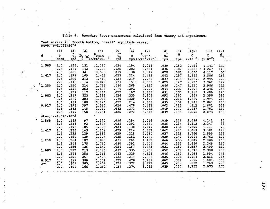
Table 4. Boundary layer parameters calculated from theory and experiment.Test series 6; Smooth bottom, "small" amplitude waves. ot=0, v=1.028xi0“3

d(1)T(sec)

(2)/\

* U °fps(3) (4)

~cmaxft2xl0-3(5)uofps

(6)Ufps

(7)Tomax

lVft2xlO“3(8)★Uofos

(9)Aufps

• (i0>C(xlO-2)

(11)C

(xlO-2)(12)A

1.565 1.0 .153 ,, 131 . 1.097 .024 .194 3.016 .039 .152 2.454 4.141 1301.5 .181 142 1.299 .026 .202 2.564 .035 .182 2.026 • 3.247 1432.0 .083 34 0.596 .017 .138 1.517 .028 .081 4.690 4.117 331.417 1.0 .197 169 1.416 .027 .224 3.482 .042 .197 1.885 3.586 1691.5 .206 213 1.483 .028 .219 2.780 .037 .215 '■ 1.657- 2.995 222’ 1.250

2.0 .118 • 114 0.849 .021 .151 1.660 .029 .127 2.720 3.762 1221.0 .250 214 1.795 .030 .269 4.182 .046 .247 1.520 2.986 2111.5 .228 253 1.636 .029 .292 3.707 .044 .230 1.598 2.246 2552.0 .127 117 0.911 .022 .167 1.835 .031 .130 2.786 3.400 120

1.083 1.0 .287 323 1.286 .026 .335 5.208 .052 .280 .847 2.398 313' 1.5 .246 203 1.765 .030 .329 4.176 .046 .261 1.339 1.994 2162.0 .131 108 0.941 .022 .214 2.353 .035 .158 1.948 2.861 130

0.917 1.0 .298 297 •1.367 .026 .478 7.432 .062 .295 .812 1.681 3561.5 .282 145 2.027 .032 .372 4.722 .049 .270 1.437 1.763 139

0t=ir,2.0 .176

V=*l. 028x10-5150 1.261

«.026 .274 ‘ 3.01-2 .039 .156 2.678 2.073 133

1.565 1.0 .185 97 1.327 .026 .1-94 3.016 .039 .166 2.489 4.141 871.5 .214 92 1.538 .028 .202 2.564 .036 .194 2.112 .3.247 832.0 .153 105 1.098 .024 .138 • 1.517 .028 .131 3.306 4.117 90

1.417 1.0 .223 143 1.602 .029 .224 3.482 .042 .200 2.069 3.586 1281.5 .225 129 1.619 .029 .219 2.780 .037 .218 1.760 2.995 1252.0 .168 129 1.205 .025 .151 1.660 .029 .142 3.088 3.762 109

1.250 1.0 .264 187 1.896 .031 .269 4.182 .046 .233 1.805 2.986 1651.5 .244 175 1.750 .030 .292 3.707 .044 .232 1.680 2.246 1672.0 .159 136 1.143 .024 .167 1.835 .031 .152 . 2.557 3.400 130

1.083 1.0 . .292 213 2.096 .032 .335 5.208 .052 .279 1.391 2.398 2031.5 .274 258 1.965 .032 .329 4.176 .046 .263 1.468 1.994 2482.0 .208 251 1.495 .028 .214 2.353 .035 .178 2.438 2.861 215

0.917 1.0 .315 380 1.501 .027 .478 7.432 .062 • .301 .856 1.681- 3631:5 ;308 305 1.439 .028 .• .• 372 4.722 ,049 ,299 .832 1.763 296• 2.0 .194 166 i. 392 .027 .274 3.012 .039 .205 1.712 2.073 175

192

Table 4. Boundary layer parameters calculated from theory and experiment.Test series 7; Hough bottom, "large" amplitude waves. ot=0, V=0.997xlO“*d T

(sec)s\Uofps

IR r Tomax (lb/ft2xlO"*) USfps Ufns

—omax(lb/ft2>:10“*) 38fps

Ufps

Ucz0 3Rr c ,(xlO 2)u*DV

1.565 1.0 .354 1301 1.829 .031 .373 • 5.711 .054 .337 43.6 1236 . 13.41 1131.5 .387 1420 2.134 .032 .412 5.151 .052 .357 69.3 1309 9.85 1142.0 .306 1124 1.417 .028 .311 3.367 .042 .277 71.7 1016 9.70 1031.417 1.0 .384 1410 2.106 .034 .442 6.767 .059 .356 46.1 1306 12.92 1221.5 .415 1522 2.407 .034 .479 5.988 .056 .386 74.9 1416 9.40 1222.0 .319 1173 1.527 . .028 .376 4.071 .046 .306 79.2 1123 9.00 100

1.250 1.0 .462 1695 2.906 .039 .547 8.375 '.066 .424 54.9 1555 11.56 1391.5 .480 1762 3.110 .040 .506 6.325 .057 .448 87.0 1644 8.50 143' 2.0 .339 1245 1.615 .029 .435 4.709 .049 .328 84.9 1203 8.70 1041.083 1.0 .519 1907 3.572 .042 .689 10.549 .074 .466- 60.3 1709 10.80 1541.5 .501 1838 3.350 .042 .693 8.663 .067 .488 94.8 1790 8.01 1542.0 .376 1381 2.031 .033 .505 5.467 .053 .389 100.0 1427 7.77 118 •0.917 1.0 .522 1916 3.636 .043 .891 13.642 .034 .538 69.6 1974 9.84 1541.5 .526 1975 3.798 .044 .793 9.914 .071 .530 102.9 1944 7.65 154 •2.0 .418

v-1.018x10"51533 2.443 .035 .594 6.431 .058 .404 104.6 1482 7.50 125

1.565 1.0 .389 1430 2.170 .033 .373 5.771 .054 .372 48.1 1336 12.65 1161.5 . .407 1491 2.338 .034 .412 5.204 .052 .411 79.8 1477 9.08 1151.417 2.0 .359 1316 1.876 .031 .311 3.402 .042 .330 85.4 1186 8.60 1091.0 .438 1574 2.664 .037 .442 6.838 .059 .400 51.8 1437 12.23 1291.5 .432 1552 2.599 .037 .479 6.051 .056 .415 80.6 1491 8.92 1292.0 .286 1027 1.261 .026 .376 4.113 .046 .306 79.2 109:9 8.40 911.250 1.0 .474 1705 3.063 .039 .547 8.463 .066 .503 65.1 1829 10.30 1361.5 .424 1525 2.520 .036 .506 6.392 .057 .426 82.7 1531 3.83 1262.0 .350 1259 1.801 .031 .435 4.759 .049 .341 83.3 1225 8.10 1091.083 1.0 .523 1880 3.635 .043 .689 10.659 .074 .530 68.6 1904 9.86 1511.5 .461 1657 2.912 .039 .693 8.754 .067 .460 89.3 1653 8.42 1362.0 .381 1369 2.085 .033 -.505 5.525 .053 .426 110.3 1531 7.28 1160.917 1.0 .537 1931 3.809 .044 .891 13.785 .084 .538 69.6 1933 9.80 154.. . 1.5 .458 1645 2.877 .038 .793 10.017 .072 .496 96.3 1782 7.90 1332.0 .409 1472 2.369 .034 .594 6.498 .058 .448 116.0 1610 7.05 119

193

Table 4. Boundary layer parameters calculated from theory and experiment.Test aeries 8: Rough bottom, "small" amplitude waves,ot - 0, V o 1.024x10“*d T(sec) Uofps IRR Tomax(lb/ft2xl0”*) **ofps Ufps Tomax (lb/ft2 xlO”*) -u sxps Ufps "

UZn

ERr C(xlO-2) ugpV

1.565 1.0 .156 558 1.438 .015 .176 2.736 .037 .136 17.6 486 24.60 531.417

1.52.0 .146.059 522211 0.3390.080 .013.006 .195.131 2.4701.437 .035.028 .147

.114 28.529.5 525

407 17.9217.7 4521631.0 .202 721 0.687 .018 .206 3.202 .040 .195 25.2 696 19.731.5 .216 771 0.772 .019 • .196 2.433 .036 .165 32.0 589 15.62 to O

1.250 2.0 . 116 • 414 0.083 .006 .150 1.646 .029 .118 30.5 421 17.35 2 11.0 .223 797 0.819 .021 .261 4.058 .046 .220 28.5 786 17.92 751.5 .226 808 0.839 .021 .250 3.167 .040 .226 43.9 807 13.25 731.0S3 2.0 .137 489 0.348 .013 .168 1.S43 .031 .136 35.2 486 15.61 731.0 .287 1027 1.276 .026 .360 5.597 .054 .255 33.0 911 16.3 901.5 .267 953 1.119 .024 .334 4.232 .047 .273 53.0 975 11.65 840.917 2.0 . 118 422 0.348 .013 .201 2.205 .033 .126 32.6 450 15.59 1031.0 .331 1182 1.633 .029 .425 6.603 .058 .309 40.0 1104 14.38 1011.5 .295 1055 1.132 .024 .362 . 4.586 .048 .283 54.9 1011 11.74 84«sfc “ IT,

2.0 v =

.142 509 1.018xl0“s

0.374«.

.014 .264 2.896 .039 .153 39.6 546 14.42 491.565 1.0 .207 742 . 0.715 .019 .176 2.723 .037 .200 25.9 718 19.68 661.5 .213 764 0.818 .021 .195 2.463 .035 .213 41.3 765 14.0 741.417 2.0 .176 631 0.538 .017 .131 1.433 .028 .171 44.3 614 13.10 611.0 .217 780 0.780 .019 .206 3.187 .040 .206 26.7 740 18.70 661.5 .226 814 0.838 .021 .196 2.476 .036 .227 44.1 815 13.00 741.250 2.0 .173 622 0.525 .017 .150 1.641 .029 .164 42.5 539 13.70 611.0 .261 939 1.079 .024 .261 4.038 .046 .248 32.1 891 15.60 841.5 .231 830 0.869 .021 .250 3.15S .040 .248 48.1 891 12.65 741.083 2.0 .156 561 0.438 .015 .168 1.838 .031 .157 40.6 564 14.25 521.0 .289 1041 1.291 .026 .360 5.569 .054 .289 37.4 1038 14.97 911*5 .290 1042 1.294 .026 ' .334 4.219 .047 .283 54.9 1016 11.74 910.917 2.0 .200 719 0.676 .013 .201 2.199 .033 .193 50.0 693 12.35 631.0 .369 1326 1.972 .032 .425 6.575 .058 .363 47.0 1304 12.77 1121.5 . 351 1260 1.806 .030 . .362 4.573 .048 .346 67.2 1243 9.91 1052.0 .238 855 0.916 .022 .264 2.888 .039 .250 64.7 898 10.38 77

VITA

Paul Geza Teleki was born in Budapest, Hungary in 19 37. His secondary education was completed at the Piarist Fathers' School in Budapest in 1956. In 1961 he obtained the degree of Bachelor of Science in • geology and in 1966 the Master of Science in geology at the University of Florida.

E X A M IN A T IO N A N D T H E S IS R E P O R T

Candidate: Paul Geza Teleki

Major Field: Geology

Title of Thesis: Measurement of boundary shear in oscillating flow in presence of roughness

Approved:

4lajor Professor and Chairman

Dean ofihe Graduate School

EXAMINING COMMITTEE:

Date of Examination:

b/z-ho