measurement error 1 in this sequence we will investigate the consequences of measurement errors in...
TRANSCRIPT

MEASUREMENT ERROR
1
In this sequence we will investigate the consequences of measurement errors in the variables in a regression model. To keep the analysis simple, we will confine it to the simple regression model.
vZY 21 wZX

2
We will start with measurement errors in the explanatory variable. Suppose that Y is determined by a variable Z, but Z is subject to measurement error, w. We will denote the measured explanatory variable X.
MEASUREMENT ERROR
vZY 21 wZX

uX
wvX
vwXY
21
221
21 )(
vZY 21 wZX
3
Substituting for Z from the second equation, we can rewrite the model as shown.
MEASUREMENT ERROR

uX
wvX
vwXY
21
221
21 )(
vZY 21 wZX
4
We are thus able to express Y as a linear function of the observable variable X, with the disturbance term being a compound of the disturbance term in the original model and the measurement error.
wvu 2
MEASUREMENT ERROR

uX
wvX
vwXY
21
221
21 )(
w w
vZY 21 wZX
5
However if we fit this model using OLS, Assumption B.7 will be violated. X has a random component, the measurement error w.
MEASUREMENT ERROR

6
And w is also one of the components of the compound disturbance term. Hence u is not distributed independently of X.
uX
wvX
vwXY
21
221
21 )(
w w
MEASUREMENT ERROR
vZY 21 wZX

7
We will demonstrate that the OLS estimator of the slope coefficient is inconsistent and that in large samples it is biased downwards if 2 is positive, and upwards if 2 is negative.
vZY 21 wZX
uXY 21 wvu 2
MEASUREMENT ERROR
2222
22121
22
XX
uuXX
XX
uuXXXX
XX
uXuXXX
XX
YYXXb
i
ii
i
iii
i
iii
i
ii

8
We begin by writing down the OLS estimator and substituting for Y from the true model. In this case there are alternative versions of the true model. The analysis is simpler if you use the equation relating Y to X.
MEASUREMENT ERROR
2222
22121
22
XX
uuXX
XX
uuXXXX
XX
uXuXXX
XX
YYXXb
i
ii
i
iii
i
iii
i
ii
vZY 21 wZX
uXY 21 wvu 2

9
Simplifying, we decompose the slope coefficient into the true value and an error term as usual.
2222
22121
22
XX
uuXX
XX
uuXXXX
XX
uXuXXX
XX
YYXXb
i
ii
i
iii
i
iii
i
ii
MEASUREMENT ERROR
vZY 21 wZX
uXY 21 wvu 2

10
We have reached this point many times before. We would like to investigate whether b2 is biased. This means taking the expectation of the error term.
MEASUREMENT ERROR
2222
XX
uuXX
XX
YYXXb
i
ii
i
ii
vZY 21 wZX
uXY 21 wvu 2

11
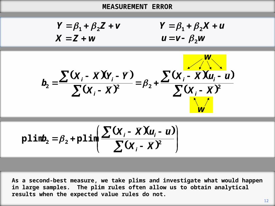
However, it is not possible to obtain a closed-form expression for the expectation of the error term. Both its numerator and its denominator are functions of w and there are no expected value rules that can allow us to simplify.
MEASUREMENT ERROR
w
w
2222
XX
uuXX
XX
YYXXb
i
ii
i
ii
vZY 21 wZX
uXY 21 wvu 2
12
As a second-best measure, we take plims and investigate what would happen in large samples. The plim rules often allow us to obtain analytical results when the expected value rules do not.
222 plim plimXX
uuXXb
i
ii
MEASUREMENT ERROR
w
w
2222
XX
uuXX
XX
YYXXb
i
ii
i
ii
vZY 21 wZX
uXY 21 wvu 2

13
We focus on the error term. We would like to use the plim quotient rule. The plim of a quotient is the plim of the numerator divided by the plim of the denominator, provided that both of these limits exist.
MEASUREMENT ERROR
22
222
1
1
plim
plim plim
XXn
uuXXn
XX
uuXXb
i
ii
i
ii
vZY 21 wZX
uXY 21 wvu 2
BA
BA
plim plim
plim
if A and B have probability limits
and plim B is not 0.

14
However, as the expression stands, the numerator and the denominator of the error term do not have limits. The denominator increases indefinitely as the sample size increases. The nominator has no particular limit.
MEASUREMENT ERROR
22
222
1
1
plim
plim plim
XXn
uuXXn
XX
uuXXb
i
ii
i
ii
vZY 21 wZX
uXY 21 wvu 2
BA
BA
plim plim
plim
if A and B have probability limits
and plim B is not 0.

15
To deal with this problem, we divide both the numerator and the denominator by n.
22
222
1
1
plim
plim plim
XXn
uuXXn
XX
uuXXb
i
ii
i
ii
MEASUREMENT ERROR
BA
BA
plim plim
plim
if A and B have probability limits
and plim B is not 0.
vZY 21 wZX
uXY 21 wvu 2

16
It can be shown that the limit of the numerator is the covariance of X and u and the limit of the denominator is the variance of X.
uXuuXXn ii ,cov1
plim
XXXn i var1
plim 2
XuX
XXn
uuXXnb
i
ii
var,cov
1
1
plim plim2
22
MEASUREMENT ERROR
vZY 21 wZX
uXY 21 wvu 2

17
Hence the numerator and the denominator of the error term have limits and we are entitled to implement the plim quotient rule. We need var(X) to be non-zero, but this will be the case assuming that there is some variation in X.
MEASUREMENT ERROR
uXuuXXn ii ,cov1
plim
XXXn i var1
plim 2
XuX
XXn
uuXXnb
i
ii
var,cov
1
1
plim plim2
22
vZY 21 wZX
uXY 21 wvu 2

22
2
2222 )var(,cov
plimwZ
w
XuX
b
22
22
2
000
,cov,cov,cov,cov
,cov,cov
w
wwwZvwvZ
wvwZuX
vZY 21 wZX
uXY 21 wvu 2
18
We can decompose both the numerator and the denominator of the error term. We will start by substituting for X and u in the numerator.
MEASUREMENT ERROR

22
2
2222 )var(,cov
plimwZ
w
XuX
b
22
22
2
000
,cov,cov,cov,cov
,cov,cov
w
wwwZvwvZ
wvwZuX
vZY 21 wZX
uXY 21 wvu 2
19
We expand the expression using the first covariance rule.
MEASUREMENT ERROR

20
If we assume that Z, v, and w are distributed indepndently of each other, the first 3 terms are 0. The last term gives us –2w
2.
MEASUREMENT ERROR
22
2
2222 )var(,cov
plimwZ
w
XuX
b
22
22
2
000
,cov,cov,cov,cov
,cov,cov
w
wwwZvwvZ
wvwZuX
vZY 21 wZX
uXY 21 wvu 2

22
2
2222 )var(,cov
plimwZ
w
XuX
b
22
22
2
000
,cov,cov,cov,cov
,cov,cov
w
wwwZvwvZ
wvwZuX
0
,cov2varvarvarvar22
wZ
wZwZwZX
vZY 21 wZX
uXY 21 wvu 2
21
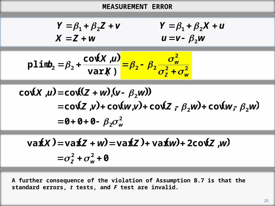
We next expand the denominator of the error term. The first two terms are variances. The covariance is 0 if we assume w is distributed independently of Z.
MEASUREMENT ERROR

22
Thus in large samples, b2 is biased towards 0 and the size of the bias depends on the relative sizes of the variances of w and Z.
MEASUREMENT ERROR
22
2
2222 )var(,cov
plimwZ
w
XuX
b
22
22
2
000
,cov,cov,cov,cov
,cov,cov
w
wwwZvwvZ
wvwZuX
0
,cov2varvarvarvar22
wZ
wZwZwZX
vZY 21 wZX
uXY 21 wvu 2

23
Since b2 is an inconsistent estimator, it is safe to assume that it is biased in finite samples as well.
MEASUREMENT ERROR
22
2
2222 )var(,cov
plimwZ
w
XuX
b
22
22
2
000
,cov,cov,cov,cov
,cov,cov
w
wwwZvwvZ
wvwZuX
0
,cov2varvarvarvar22
wZ
wZwZwZX
vZY 21 wZX
uXY 21 wvu 2

24
If our assumptions concerning Z, v, and w are incorrect, b2 would almost certainly still be an inconsistent estimator, but the expression for the large-sample bias would be more complicated.
MEASUREMENT ERROR
22
2
2222 )var(,cov
plimwZ
w
XuX
b
22
22
2
000
,cov,cov,cov,cov
,cov,cov
w
wwwZvwvZ
wvwZuX
0
,cov2varvarvarvar22
wZ
wZwZwZX
vZY 21 wZX
uXY 21 wvu 2
25
A further consequence of the violation of Assumption B.7 is that the standard errors, t tests, and F test are invalid.
MEASUREMENT ERROR
22
2
2222 )var(,cov
plimwZ
w
XuX
b
22
22
2
000
,cov,cov,cov,cov
,cov,cov
w
wwwZvwvZ
wvwZuX
0
,cov2varvarvarvar22
wZ
wZwZwZX
vZY 21 wZX
uXY 21 wvu 2

26
The analysis will be illustrated with a simulation. The true model is Y = 2.0 + 0.8Z + u,with the values of Z drawn randomly from a normal distribution with mean 10 and variance 4, and the values of u being drawn from a normal distribution with mean 0 and variance 4.
MEASUREMENT ERROR
Simulation
uZY 8.00.2 4,10~ NZ 4,0~ Nu
22
2
2222 )var(,cov
plimwZ
w
XuX
b
vZY 21 wZX
uXY 21 wvu 2

27
X = Z + w, where w is drawn from a normal distribution with mean 0 and variance 1. With this information, we are able to determine plim b2.
MEASUREMENT ERROR
Simulation
uZY 8.00.2 4,10~ NZ 4,0~ Nu
64.014
18.08.0 plim 22
2
222
wZ
wb
wZX 1,0~ Nw
22
2
2222 )var(,cov
plimwZ
w
XuX
b
vZY 21 wZX
uXY 21 wvu 2
28
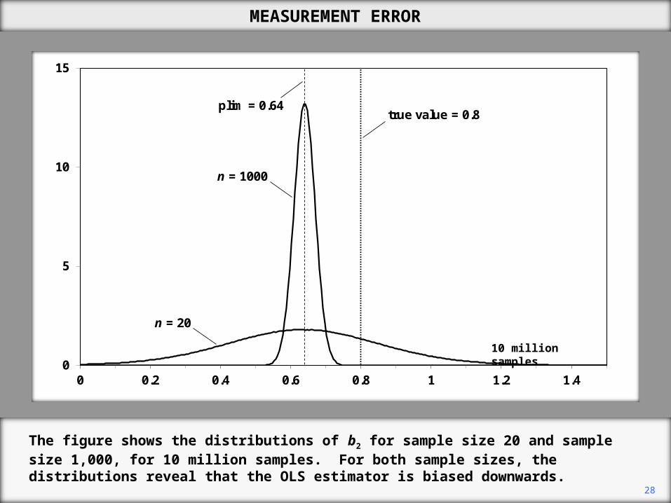
The figure shows the distributions of b2 for sample size 20 and sample size 1,000, for 10 million samples. For both sample sizes, the distributions reveal that the OLS estimator is biased downwards.
MEASUREMENT ERROR
0
5
10
15
0 0.2 0.4 0.6 0.8 1 1.2 1.4
true value = 0.8plim = 0.64
n = 1000
n = 20
10 million samples
29
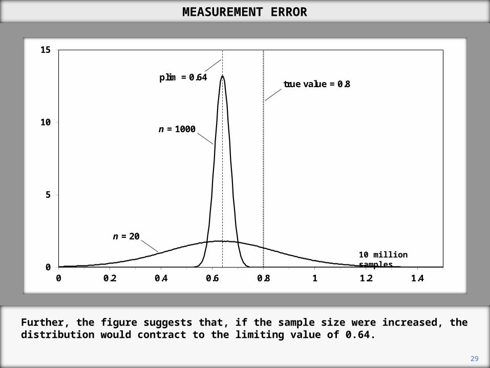
Further, the figure suggests that, if the sample size were increased, the distribution would contract to the limiting value of 0.64.
MEASUREMENT ERROR
0
5
10
15
0 0.2 0.4 0.6 0.8 1 1.2 1.4
true value = 0.8plim = 0.64
n = 1000
n = 20
10 million samples

30
There remains the question of whether the limiting value provides guidance to the mean of the distribution for a finite sample. In general, the mean will be different from the limiting value, but will approach it as the sample size increase.
MEASUREMENT ERROR
0
5
10
15
0 0.2 0.4 0.6 0.8 1 1.2 1.4
true value = 0.8plim = 0.64
n = 1000
n = 20
10 million samples

31
In the present case, however, the mean of the sample is almost exactly equal to 0.64, even for sample size 20.
MEASUREMENT ERROR
0
5
10
15
0 0.2 0.4 0.6 0.8 1 1.2 1.4
true value = 0.8plim = 0.64
n = 1000
n = 20
10 million samples

32
Measurement error in the dependent variable has less serious consequences. Suppose that the true dependent variable is Q, that the measured variable is Y, and that the measurement error is r.
MEASUREMENT ERROR
rQY vXQ 21

33
We can rewrite the model in terms of the observable variables by substituting for Q from the second equation.
MEASUREMENT ERROR
vXrY 21
rQY vXQ 21

34
In this case the presence of the measurement error does not lead to a violation of Assumption B.7. If v satisfies that assumption in the original model, u will satisfy it in the revised one, unless for some strange reason r is not distributed independently of X.
MEASUREMENT ERROR
uX
rvXY
21
21
vXrY 21
rvu
rQY vXQ 21

35
uX
rvXY
21
21
The standard errors and tests will remain valid. However the standard errors will tend to be larger than they would have been if there had been no measurement error, reflecting the fact that the variances of the coefficients are larger.
vXrY 21
2
22
2
22
2
X
rv
X
ub nn
rvu
MEASUREMENT ERROR
rQY vXQ 21

2012.11.12
Copyright Christopher Dougherty 2012.
These slideshows may be downloaded by anyone, anywhere for personal use.
Subject to respect for copyright and, where appropriate, attribution, they may be
used as a resource for teaching an econometrics course. There is no need to
refer to the author.
The content of this slideshow comes from Section 8.4 of C. Dougherty,
Introduction to Econometrics, fourth edition 2011, Oxford University Press.
Additional (free) resources for both students and instructors may be
downloaded from the OUP Online Resource Centre
http://www.oup.com/uk/orc/bin/9780199567089/.
Individuals studying econometrics on their own who feel that they might benefit
from participation in a formal course should consider the London School of
Economics summer school course
EC212 Introduction to Econometrics
http://www2.lse.ac.uk/study/summerSchools/summerSchool/Home.aspx
or the University of London International Programmes distance learning course
EC2020 Elements of Econometrics
www.londoninternational.ac.uk/lse.