DIPLOMARBEIT

Measurement Based Evaluation of

Interference Alignment on the Vienna

MIMO Testbed

Ausgeführt zum Zwecke der Erlangung des akademischen Grades eines Diplom-Ingenieursunter der Leitung von

Univ.Prof. Dipl.-Ing. Dr.techn. Markus Rupp

und

Dipl.-Ing. Martin Lerch

am

Institute of Telecommunications

eingereicht an der Technischen Universität WienFakultät für Elektrotechnik und Informationstechnik

von

Martin Mayer0725729

Blödleweg 56820 Frastanz

Wien, Oktober 2013

I hereby declare that this thesis is my original work and it has been written by me in its entirety.I have acknowledged all the sources of information which have been used in the thesis.

Martin MayerVienna, October 2013

Abstract

Most modern wireless multi-user networks suffer from undesired interference that impairs thedata transmission over the individual radio links. In order to maximize the data throughputin such systems, several interference mitigation schemes have been investigated recently. Inter-ference alignment stands out as one of the most promising ones, able to attain the maximumdata throughput over interference disturbed links in theory, given the right conditions. As thetheoretical research progresses, practical implementations have to be considered in order toconfirm the theory and discover limitations introduced by hardware.

Interference alignment utilizes linear filtering at each transmitter and receiver of the network.The transmit filters thereby partition the signal space at the receiver into two subspaces, adesired signal subspace containing the signal from the desired transmitter and an interferencesubspace accumulating all the interfering signals. The aligned interference is then forced tozero by the receive filter and only the desired signal is retained. For this to be accomplished,cooperation of all users in the network is required.

This work first deals with the theoretical foundations of interference alignment by introducingthe relevant system model and discussing feasibility and filter computation. It then advancesto the characterization of the Vienna MIMO testbed on which interference alignment wasimplemented throughout this work. The testbed employs two outdoor transmitters on rooftops,one indoor transmitter and one indoor receiver. The radio channels in the considered setupare quasi-static. Hardware, software and the used signals are described. Performance measuresfor evaluation are introduced. Finally, measurement results are presented. The feasibility ofinterference alignment is shown, and the performance measures are evaluated over variablesignal to noise ratio and variable signal to interference ratio. The results are discussed, andimpairments introduced by hardware are highlighted.

Kurzfassung

Moderne drahtlose Multiuser-Netzwerke werden oft durch unerwünschte Interferenz gestört,welche die Datenübertragung über die jeweiligen Funkverbindungen verschlechtert. EinigeMethoden zur Steigerung der Datenrate in solchen Systemen wurden kürzlich untersucht. “In-terference Alignment” sticht dabei als eines der vielversprechendsten Verfahren hervor, da es inder Theorie die maximale Datenrate erreicht, wenn die richtigen Umstände gegeben sind. Mitdem Fortschritt der theoretischen Forschung werden praktische Implementierungen relevant,damit die Theorie bestätigt und mögliche hardwarebedingte Limitationen entdeckt werden.

“Interference Alignment” verwendet lineare Sende- und Empfangsfilter. Der Signalraum amjeweiligen Empfänger wird dabei durch die Sendefilter in zwei Unterräume unterteilt, einenUnterraum für das erwünschte Signal und einen Unterraum, in dem alle Interferenz-Signaleüberlappen. Die gesammelte Interferenz wird dann mittels Empfangsfilter eliminiert und nurdas erwünschte Signal bleibt bestehen. Das Verfahren ist nur möglich, wenn alle Benutzer desNetzwerks kooperieren.

Diese Arbeit beginnt mit einer theoretischen Abhandlung von “Interference Alignment”. Dabeiwird zuerst das relevante System-Modell eingeführt, anschließend werden Voraussetzungenund Filterberechnung besprochen. Als nächstes wird das “Vienna MIMO testbed” charak-terisiert, auf welchem “Interference Alignment” im Zuge dieser Arbeit implementiert wurde.Es besteht aus zwei Outdoor-Sendeanlagen auf Häuserdächern, einer Indoor-Sendeanlage undeiner Indoor-Empfangsanlage. Die Funkkanäle sind dabei quasi-statisch. Hardware, Softwareund die benutzten Signale werden beschrieben. Performance-Maße werden eingeführt, die zurBewertung der “Interference Alignment” Qualität dienen. Anschließend werden Messergebnissepräsentiert. Die Machbarkeit von “Interference Alignment” wird gezeigt, und das Verhalten derPerformance-Maße wird untersucht, einmal für variables Signal-Rausch-Verhältnis und einmalfür variables Signal-Interferenz-Verhältnis. Beeinträchtigungen durch die verwendete Hardwarewerden aufgezeigt.

Contents

1 Introduction 11.1 The Virtues of Interference Alignment . . . . . . . . . . . . . . . . . . . . . . . 21.2 Testbed Aided Evaluation . . . . . . . . . . . . . . . . . . . . . . . . . . . . . . 41.3 Outline . . . . . . . . . . . . . . . . . . . . . . . . . . . . . . . . . . . . . . . . 5

2 System Model and Interference Alignment 62.1 K-User MIMO Interference Channel . . . . . . . . . . . . . . . . . . . . . . . . 62.2 Mutual Information and Degrees of Freedom . . . . . . . . . . . . . . . . . . . . 72.3 Interference Alignment . . . . . . . . . . . . . . . . . . . . . . . . . . . . . . . . 10

2.3.1 Feasibility . . . . . . . . . . . . . . . . . . . . . . . . . . . . . . . . . . . 112.3.2 Closed Form Solution . . . . . . . . . . . . . . . . . . . . . . . . . . . . 12

3 Vienna MIMO Testbed 133.1 Hardware and Deployment . . . . . . . . . . . . . . . . . . . . . . . . . . . . . . 13

3.1.1 Transmitter . . . . . . . . . . . . . . . . . . . . . . . . . . . . . . . . . . 153.1.2 Receiver . . . . . . . . . . . . . . . . . . . . . . . . . . . . . . . . . . . . 16

3.2 Measurement Methodology . . . . . . . . . . . . . . . . . . . . . . . . . . . . . 183.3 Signals and Channel Estimation . . . . . . . . . . . . . . . . . . . . . . . . . . . 18

3.3.1 Transmit Signals . . . . . . . . . . . . . . . . . . . . . . . . . . . . . . . 193.3.2 Receive Signals . . . . . . . . . . . . . . . . . . . . . . . . . . . . . . . . 213.3.3 Channel Estimation . . . . . . . . . . . . . . . . . . . . . . . . . . . . . 23

3.4 Software and Control . . . . . . . . . . . . . . . . . . . . . . . . . . . . . . . . . 243.4.1 Measurement . . . . . . . . . . . . . . . . . . . . . . . . . . . . . . . . . 243.4.2 Transmit Routine . . . . . . . . . . . . . . . . . . . . . . . . . . . . . . . 29

4 Evaluation and Quantities of Interest 314.1 Assumptions and Detailed Frame Structure . . . . . . . . . . . . . . . . . . . . 314.2 Measured Mutual Information . . . . . . . . . . . . . . . . . . . . . . . . . . . . 33

4.2.1 Mutual Information from Channel Estimates . . . . . . . . . . . . . . . 334.2.2 Mutual Information from Receive Data Covariance . . . . . . . . . . . . 35

4.3 Interference Suppression . . . . . . . . . . . . . . . . . . . . . . . . . . . . . . . 364.4 Power, SNR and SIR . . . . . . . . . . . . . . . . . . . . . . . . . . . . . . . . . 38

5 Measurements 405.1 Validation of Interference Alignment . . . . . . . . . . . . . . . . . . . . . . . . 405.2 Variable SNR at Fixed SIR . . . . . . . . . . . . . . . . . . . . . . . . . . . . . 47

5.2.1 Measured Powers, SNR and SIR . . . . . . . . . . . . . . . . . . . . . . 485.2.2 Interference Suppression . . . . . . . . . . . . . . . . . . . . . . . . . . . 515.2.3 Mutual Information . . . . . . . . . . . . . . . . . . . . . . . . . . . . . 53

5.3 Variable SIR at Fixed SNR . . . . . . . . . . . . . . . . . . . . . . . . . . . . . 555.3.1 Measured Powers, SNR and SIR . . . . . . . . . . . . . . . . . . . . . . 555.3.2 Interference Suppression . . . . . . . . . . . . . . . . . . . . . . . . . . . 59

i

5.3.3 Mutual Information . . . . . . . . . . . . . . . . . . . . . . . . . . . . . 62

6 Conclusion and Outlook 64

List of Figures 66

Bibliography 68

ii

Chapter 1

Introduction

Interference lowers the achievable data rates in wireless multi-user networks. Transmissionsthat naturally occupy a certain bandwidth are thereby disturbed by interferers that transmitin the same frequency band. As a result, the superposition of the signals at the receiver impairsthe desired signal, since its waveform and amplitude are altered by the interference.

Where in former times, we were able to divide applications into individual frequency bandsand thereby avoid interference, we soon reached a point where these bands were highly occupiedand the resource of frequency became scarce. The bandwidth and operational frequency of anapplication are also constrained by physical properties like antenna size. We had to come upwith new ideas to maximize the (spectral) efficiency of our wireless transmission schemes inorder to accommodate more channels in the same frequency band. Schemes that successfullymanage interference yield tremendous potential in that area.

With a steadily increasing number of users in wireless networks such as the cellular systemin mobile communications, the need of multiple access schemes emerged. Users can be distin-guished in frequency domain (designated frequency/channel), in time domain (designated timeslot), in code domain (designated signature) or in space domain (designated direction of radiobeam). The realizations of these ideas are called Frequency Division Multiple Access (FDMA),Time Division Multiple Access (TDMA), Code Division Multiple Access (CDMA) and SpaceDivision Multiple Access (SDMA), respectively. What all these multiple access schemes havein common is the effect of decreasing maximum data rate per user with increasing number ofusers. This is due to the fact that the frequency/time/code/spatial domain can not be fullyexploited for data transmission as in the single user case. The channel can be seen as a cake,and every user gets only a slice of it. A simple example illustrating this behaviour is the oneof K users that want to transmit data within one second - each user gets only the fraction 1

K

of a second to transmit its data or put differently, it takes each user K seconds to transmit thesame amount of data as in the single user case.

In cellular networks, interference will always be an issue. Despite frequency planning1,frequencies have to be reused, either in adjacent cells as in UMTS2 or in further separatedcells as in GSM3. The difference manifests itself in the strength of the interference and how itis handled. With increasing number of users, these networks ultimately become interferencelimited, meaning that an increase of transmit power does not result in better signal qualityand higher data throughput as in noise limited networks. This behaviour also applies to othermulti-user networks such as WLAN4.

1Frequency planning here refers to the downlink in a cellular system, namely the channel from serving basestation to user equipment. The so called inter-cell interference comes from neighbouring cells that operateon the same frequency as the serving cell.

2Universal System of Mobile Communications (in 3rd generation mobile networks)3Global System for Mobile Communications (in 2nd generation mobile networks)4Wireless Local Area Network, IEEE 802.11

1

Conversely to the somewhat old fashioned cake cutting analogon where every user gets only a“slice” of the channel, it has recently been shown in [1] that the maximum data rate per user isnot necessarily decreasing with increasing number of users. The refined statement claims that“every user is able to get half the cake”, the rate-penalty of having K users communicating onthe same resource would only be 1

2 instead of 1K

. Several interference management approacheshave been researched, but Interference Alignment (IA) stands out as one of the most promisingones. As a future technology, it might be employed as an interference mitigation technique inthe further progression of LTE5.

In Section 1.1, the advances in interference management are sketched, the basic idea behind IAis explained and finally, its requirements are listed. Section 1.2 then illuminates the benefitsof testbed driven evaluation in the context of IA and compares the approaches that have beentaken up to the point where this work was written. An outline of this work is subsumed inSection 1.3.

1.1 The Virtues of Interference Alignment

The choice of the proper interference management approach heavily depends on the aspects ofthe considered system, such as the Signal to Noise Ratio (SNR) and the interference strengthwhich is usually expressed by the Signal to Interference Ratio (SIR). Three classic approachesare now listed, loosely following the introduction in [1]:

• Treat as noise: In case of weak interference, the interfering signals can be treated asnoise. Single user encoding and decoding is performed. However, this approach is sub-optimal from an information theoretic point of view since the structure in the interferingsignals is not exploited.

• Orthogonalized access: In case of interference being about as strong as the desiredsignal, it can be avoided by orthogonalizing the channel access with multiple accessschemes. This is the “cake cutting” approach where every user accessing the medium getsonly a “slice”.

• Decode: In case of strong interference, the interfering signals might be decoded alongwith the desired signal. While improving the data rate of the desired user, the interferingusers experience lowered rates due to the necessary overhead for multi-user detection.

Interference Alignment (IA) addresses the case where interference and desired signal are aboutequally strong. It redeems the “cake cutting” approach and - given the right conditions - is ableto serve every user “half the cake”. This results in heavily increased data rates in multi-usersystems.

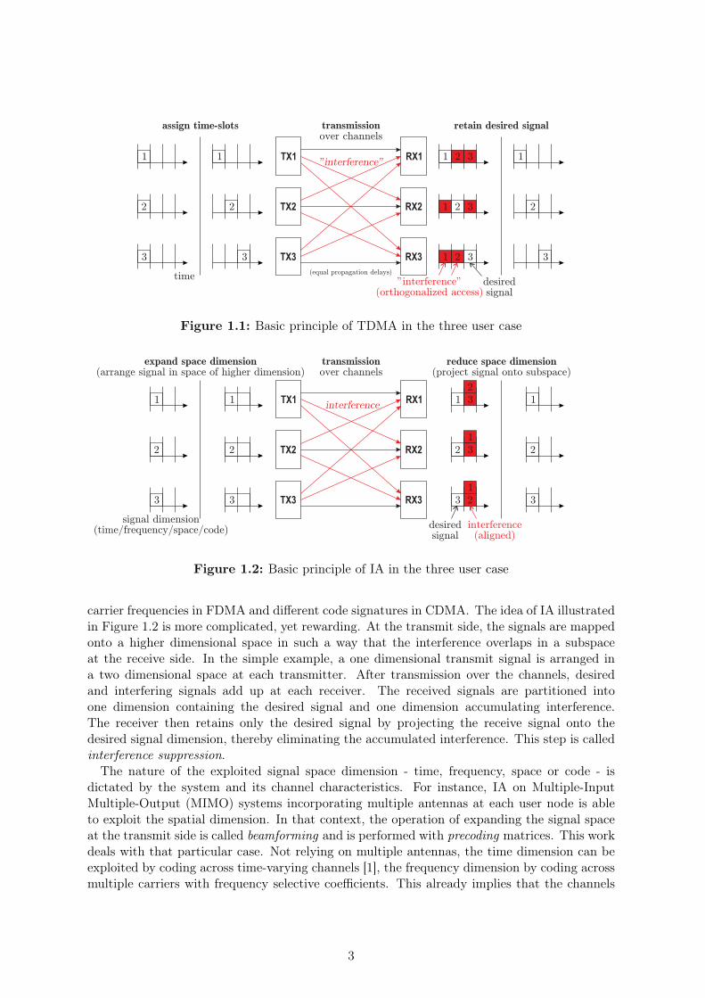
Consider such a multi-user system with three transmitter-receiver pairs (users) where eachtransmitter wants to communicate only with its corresponding (desired) receiver. Each userreceives two interfering signals on top of the desired signal. The approach using TDMA isdepicted in Figure 1.1. Each user is assigned to a designated time slot. In the example, allpropagation delays are equal and no inter-symbol interference occurs. At the receive side,the signals can be separated perfectly. However, the time until every user is served linearlyincreases with the number of users. Equivalently, the users could be separated on different

53GPP Long Term Evolution (in 4th generation mobile networks)

2

"interference"1 11 1

1

1

2 22

2

2

23 33

3

3

3

time

assign time-slots transmissionover channels

retain desired signal

TX1

TX2

TX3

RX1

RX2

RX3

(equal propagation delays)

"interference"(orthogonalized access)

desiredsignal

Figure 1.1: Basic principle of TDMA in the three user case

interference1 1 1 1

1

1

2 2 2 2

2

2

3 3 3 3

3

3

signal dimension(time/frequency/space/code)

expand space dimension(arrange signal in space of higher dimension)

transmissionover channels

reduce space dimension(project signal onto subspace)

TX1

TX2

TX3

RX1

RX2

RX3

interference(aligned)

desiredsignal

Figure 1.2: Basic principle of IA in the three user case

carrier frequencies in FDMA and different code signatures in CDMA. The idea of IA illustratedin Figure 1.2 is more complicated, yet rewarding. At the transmit side, the signals are mappedonto a higher dimensional space in such a way that the interference overlaps in a subspaceat the receive side. In the simple example, a one dimensional transmit signal is arranged ina two dimensional space at each transmitter. After transmission over the channels, desiredand interfering signals add up at each receiver. The received signals are partitioned intoone dimension containing the desired signal and one dimension accumulating interference.The receiver then retains only the desired signal by projecting the receive signal onto thedesired signal dimension, thereby eliminating the accumulated interference. This step is calledinterference suppression.

The nature of the exploited signal space dimension - time, frequency, space or code - isdictated by the system and its channel characteristics. For instance, IA on Multiple-InputMultiple-Output (MIMO) systems incorporating multiple antennas at each user node is ableto exploit the spatial dimension. In that context, the operation of expanding the signal spaceat the transmit side is called beamforming and is performed with precoding matrices. This workdeals with that particular case. Not relying on multiple antennas, the time dimension can beexploited by coding across time-varying channels [1], the frequency dimension by coding acrossmultiple carriers with frequency selective coefficients. This already implies that the channels

3

have to be uncorrelated (i.e. full rank channel matrices in MIMO transmissions) for optimalresults. To realize the separation of desired signal and interference at the receiver, overallchannel knowledge is required. Only then, the signals can be precoded at the transmit side sothat interference aligns at the receive side. The users therefore need the ability to communicatewith each other (i.e. feedback). By cooperation of all user nodes, a jointly optimal beamformingscheme called IA is possible. Furthermore, the 1

2 rate penalty (“every user gets half the cake”)is only attained in the high SNR regime.

1.2 Testbed Aided Evaluation

The foundation of scientific innovation is based on ideas that develop into theories followed bymathematical descriptions and models. As soon as we are able to imagine how something couldwork, we start to abstract the problem. Especially at the beginning, this might lead to veryconceptional drafts that are far from reality and can not directly be applied in the real world.Section 1.1 dealt with a similar case and explained the principles of IA in a very abstract way.

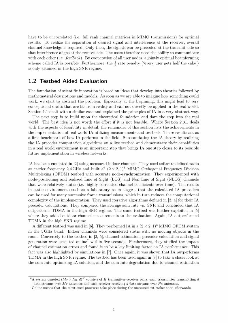
The next step is to build upon the theoretical foundation and dare the step into the realworld. The best idea is not worth the effort if it is not feasible. Where Section 2.3.1 dealswith the aspects of feasibility in detail, the remainder of this section lists the achievements inthe implementation of real world IA utilizing measurements and testbeds. These results act asa first benchmark of how IA performs in the field. Substantiating the IA theory by realizingthe IA precoder computation algorithms on a live testbed and demonstrate their capabilitiesin a real world environment is an important step that brings IA one step closer to its possiblefuture implementation in wireless networks.

IA has been emulated in [2] using measured indoor channels. They used software defined radioat carrier frequency 2.4GHz and built a6 (2× 2, 1)3 MIMO Orthogonal Frequency DivisionMultiplexing (OFDM) testbed with accurate node-synchronization. They experimented withnode-positioning and realized Line of Sight (LOS) and Non Line of Sight (NLOS) channelsthat were relatively static (i.e. highly correlated channel coefficients over time). The resultsin static environments such as a laboratory room suggest that the calculated IA precoderscan be used for many successive frame transmissions, which in turn reduces the computationalcomplexity of the implementation. They used iterative algorithms defined in [3, 4] for their IAprecoder calculations. They compared the average sum rate vs. SNR and concluded that IAoutperforms TDMA in the high SNR regime. The same testbed was further exploited in [5]where they added outdoor channel measurements to the evaluation. Again, IA outperformedTDMA in the high SNR regime.

A different testbed was used in [6]. They performed IA in a (2× 2, 1)3 MIMO OFDM systemin the 5GHz band. Indoor channels were considered static with no moving objects in theroom. Conversely to the testbed in [2, 5], channel estimation, precoder calculation and signalgeneration were executed online7 within five seconds. Furthermore, they studied the impactof channel estimation errors and found it to be a key limiting factor on IA performance. Thisfact was also highlighted by simulations in [7]. Once again, it was shown that IA outperformsTDMA in the high SNR regime. The testbed has been used again in [8] to take a closer look atthe sum rate optimizing IA solution, and the sum rate degradation due to channel estimation

6A system denoted (MT ×NR, d)K consists of K transmitter-receiver pairs, each transmitter transmitting d

data streams over MT antennas and each receiver receiving d data streams over NR antennas.7Online means that the mentioned processes take place during the measurement rather than afterwards.

4

error was demonstrated.Where it took the testbeds in [6, 8] roughly five seconds for computations between frame

transmissions, the testbed in [9] reduces this time to the tenth of a second. They built a movabletestbed operating at 2.49GHz that constitutes a (2× 2, 1)3 MIMO OFDM system. Variousindoor positions for the mobile stations were considered. IA was compared to coordinatedmultipoint with ideal and measured results. The gains over the reference schemes of thesingle user MIMO case achieved by measurements were much smaller than stated by theory,which was presumably caused by spurious Radio Frequency (RF) effects. Nevertheless, IA andcoordinated multipoint outperformed the reference schemes of the single user MIMO case, suchas TDMA.

1.3 Outline

In this work, the Vienna MIMO Testbed (VMTB) is used to demonstrate the feasibility of In-terference Alignment (IA) in a (4× 4, 2)3 MIMO OFDM system at carrier frequency 2.5GHz.A heterogeneous urban scenario consisting of two outdoor transmitters, one indoor transmitterand one indoor receiver is investigated. The channels are considered static, the receive antennasare mounted on a x-y-φ table to create different channel realizations. Precoder computationand signal generation are performed online within approximately 70ms. Aside from the feasi-bility demonstration, the impact of variable SNR and SIR on the data rate is observed. Thefirst IA results utilizing this testbed setup were published in [10].

This work is structured as follows. Chapter 2 introduces the underlying system model andexplains how the mutual information (representing the possible data rate) is obtained, withand without IA. It then discusses the role of the Degrees of Freedom (DoF) and advancesto the principles of IA. Chapter 3 deals with the VMTB in detail. Hardware, software, theprinciples of measurement and the used signals are explained. Chapter 4 introduces measuresfor the evaluation of measurements. Chapter 5 shows the measurement results and discussestheir implications. Chapter 6 subsumes the work and gives an outlook.

5

Chapter 2

System Model and Interference Alignment

The system model representing the basis of further characterizations is introduced in Sec-tion 2.1. Section 2.2 then compares how mutual information and the Degrees of Freedom (DoF)behave with and without Interference Alignment (IA). Based upon these fundamentals, Sec-tion 2.3 deals with the theory behind IA and how it is applied. Note that if not stated otherwise,the considered models are the ones used for IA.

2.1 K-User MIMO Interference Channel

The K-user MIMO interference channel comprises K transmitter-receiver pairs (also calledlinks), where each receiver suffers from K − 1 interferers. This work restricts itself to thesymmetric case, where every transmitter has MT antennas and every receiver has NR anten-nas. Furthermore, each link communicates on d data streams. Such a system is denoted as(MT ×NR, d)

K . An exemplary (4× 4, 2)3 system is depicted in Figure 2.1.

TX2

TX3

TX1 RX1

RX2

RX3

Figure 2.1: (4× 4, 2)3 MIMO interference channel

Each transmitter, indexed by j ∈ {1, ...,K}, transmits a data stream sj ∈ Cd that is beam-

formed by applying a truncated unitary precoding matrix Vj ∈ CMT×d according to

xj = Vjsj , (2.1)

where xj ∈ CMT constitutes the transmit signal vector. Let i ∈ {1, ...,K} denote the receiver

index. The transmit signal vector is transmitted over the respective channels whose coefficientsare stored in channel matrices Hij ∈ C

NR×MT . At the ith receiver, the noise vector ni ∈ CNR

6

is added, which is (for simplicity in the following) assumed to be circularly symmetric complexGaussian i.i.d.1 with zero mean and variance σ2

ni, ni ∼ CN (0, σ2

niINR

). The receive signalvector yi ∈ C

NR , obtained as

yi =K∑

j=1

Hij Vjsj︸ ︷︷ ︸xj

+ni, (2.2)

is then filtered by the truncated unitary interference suppression matrix Ui ∈ CNR×d according

to

ri = UHi yi =

K∑

j=1

UHi HijVjsj +UH

i ni = UHi HiiVisi︸ ︷︷ ︸

desired signal

+K∑

j=1j 6=i

UHi HijVjsj

︸ ︷︷ ︸interference

+UHi ni︸ ︷︷ ︸

noise

(2.3)

which yields the receive data stream ri ∈ Cd, an estimation of the corresponding transmit data

stream si of user i.The precoding matrices Vj and interference suppression matrices Ui are chosen to jointly

suppress the interference in Equation (2.3), their calculation is discussed in Section 2.3.2.

2.2 Mutual Information and Degrees of Freedom

Consider a MIMO link with MT transmit antennas and NR receive antennas. The receivesignal vector is obtained as y = Hx+ n, with fixed (deterministic) channel realization H andcircularly symmetric complex Gaussian i.i.d. noise vector n ∼ CN (0, σ2

nINR). The mutual

information2 between x and y is defined as [11]

I(x;y) = log2 det

(INR

+1

σ2n

HQHH

), (2.4)

where Q ∈ RMT×MT defines the power allocation at the transmit antennas and trace(Q) = P

yields the total transmit power constraint. Assuming equal transmit power PMT

at each antenna,

Q =P

MTIMT

(2.5)

and Equation (2.4) becomes

I(x;y) = log2 det(INR

+ γHHH)

(2.6)

with SNR γ = PMTσ2

n. A common approach to investigate MIMO systems is to perform a

Singular Value Decomposition (SVD)3 on the channel matrix H:

H = LΣRH. (2.7)

1The elements of an i.i.d. random vector are (statistically) independent and identically distributed.2The mutual information I(x;y) can be seen as the reduction in the uncertainty about x due to the knowledge

of y. In the information theoretic context, it corresponds to rate. Its unit is [bit/s/Hz].3A singular value decomposition A = LΣRH decomposes a matrix A ∈ C

NR×MT into a unitary matrixL ∈ C

NR×NR containing its left singular vectors, a rectangular diagonal matrix Σ ∈ RNR×MT containing

its singular values in the main diagonal and a unitary matrix RH ∈ CMT×MT containing its right singular

vectors.

7

The MIMO transmission is decomposed into NΣ parallel Single-Input Single-Output (SISO)transmissions, where NΣ is the number of nonzero singular values in Σ and NΣ = min(MT, NR)if H has full rank, which is assumed here. Decomposing H in Equation (2.6) leads to

I(x;y) = log2 det

INR

+ γLΣRHR︸ ︷︷ ︸=IMT

ΣTLH

= log2 det(INR

+ γLΣΣTLH)

= log2 det(LLH + γLΣΣTLH

)

= log2 det(L(INR

+ γΣΣT)LH)

= log2 det(INR

+ γΣΣT)

=

min(MT,NR)∑

s=1

log2 (1 + γλs) ,

(2.8)

where the squared singular values in ΣΣT = diag{λ1, ..., λmin(MT,NR)} are the eigenvalues of

HHH, denoted λs. The Degrees of Freedom (DoF) are now defined as

DoF = limγ→∞

I(x;y)log2 γ

=

min(MT,NR)∑

s=1

limγ→∞

log2 (1 + γλs)

log2 γ

=

min(MT,NR)∑

s=1

limγ→∞

γ

1 + γ︸ ︷︷ ︸=1

= min(MT, NR).

(2.9)

In a MIMO system, the DoF are also called multiplexing gain since the link capacity growslinearly with the number of antennas min(MT, NR).

The transition to the interference channel introduced in Section 2.1 is now discussed. Insteadof one single MIMO link, K links exist, and each user receives interference on top of the desiredsignal. Assuming perfect IA that nulls the interference terms in Equation (2.3), the receivestream ri will be interference free. The resulting transmission of information takes place overthe interference free channel UH

i HiiVi of reduced rank d < rank(Hii). This way, each linkis interference free and can be viewed as stand-alone MIMO link as in the beginning of thissection. The link index i is now dropped and the mutual information over an interferencealigned link becomes4

I(s; r) = log2 det

(Id +

1

σ2n

(UHHV)Q(UHHV)H). (2.10)

Taking the same assumptions and steps as in the interference free case, this develops into

I(s; r) =d∑

s=1

log2 (1 + γλs) . (2.11)

4Note that Q = P

dId, since power is now allocated on d data streams rather than MT antennas.

8

The DoF in the interference aligned case are

DoFIA = limγ→∞

I(s; r)log2 γ

= d < min(MT, NR). (2.12)

IA therefore renders a system interference free at the expense of reduced DoF respectivelymultiplexing gain. The computation of the mutual information in the non-ideal IA case (i.e.non-perfect channel knowledge) is discussed in Section 4.2.

A capacity characterization for the K-user interference channel is not straight-forward. The fol-lowing summary relates to K-user interference channels with single antenna nodes (not MIMO).The K = 2-user Gaussian interference channel was studied in [12] and capacity bounds wereproposed. In [13], it was shown that the maximum achievable DoF of a network involvingK = 2 users is one (12 per user) and they inferred that for K users, it is at most K

2 (12 peruser). The landmark paper [1] coincides with that result and characterizes the sum capacityof the K-user interference channel as C(γ) = K

2 log2(γ) +O(log2(γ)), where O(log2(γ)) is anapproximation error. This result is shown to be achievable almost surely in the case of time-varying channel coefficients and beamforming over multiple symbol extensions.

This work focuses on the symmetric square (MT = NR) K = 3-user MIMO interference channelwith quasi-static channel coefficients, since these circumstances are experienced in the mea-surements (Chapter 5). It was shown in [1] that the sum capacity in this case is characterized(almost surely) as C(γ) = 3

2NR log2(1 + γ) +O(1). The total DoF are hence 32NR = K

2 NR,and the per user DoF are 1

2NR which is half the DoF a user could achieve in the absence ofinterference (see Equation (2.9)). This is a major improvement over classical orthogonalizationapproaches like TDMA where the per user DoF are given as 1

KNR and are hence decreasing

with increasing number of users. This result also holds true5 for larger number of users K andis the essence behind the “every user gets half the cake” statement. However, it is only validat high SNR. The scheme achieving this is called Interference Alignment (IA) and will now bediscussed.

5Requirements see [1]. A larger number of users K requires a larger signal space.

9

2.3 Interference Alignment

Interference Alignment (IA) is the scheme proposed to maximize the achievable Degrees ofFreedom (DoF) in an interference channel. In a MIMO system, the DoF correspond to theachievable multiplexing gain (see Section 2.2). Considering an interference channel, they canbe interpreted as follows:

• The DoF of wireless interference networks represent the number of interference-free sig-naling dimensions in the network [14].

• The maximum total DoF correspond to the first-order approximation of sum-rate capacityin the high SNR regime [15].

By maximizing the DoF, intuitively the achievable data rate is also maximized. IA is cur-rently seen to be the optimal scheme that approaches the Shannon capacity [16] of interferencenetworks in the high SNR regime.

The realization of IA basically boils down to the computation of precoding matrices Vj andinterference suppression matrices Ui that jointly suppress the interference (see Equation (2.3))in the K-user MIMO interference channel introduced in Section 2.1. To that end, followingtwo conditions have to be satisfied simultaneously:

UHi HijVj = 0, ∀j 6= i (2.13a)

rank(UHi HiiVi) = d, ∀i ∈ {1, ...,K}. (2.13b)

These conditions already imply that the channel matrices Hij have to be known in order tocompute Vj , Ui.

The precoding matrices Vj applied at transmitters j = {1, ...,K} are designed to maximizethe overlap of the interference signal subspaces at each receiver while ensuring that the desiredsignal vectors at each receiver are linearly independent of the interference subspace [14].

The interference suppression matrices Ui applied at receivers i = {1, ...,K} perform zeroforcing of the interference without zero forcing the desired signal (which is linearly independentof interfering signals).

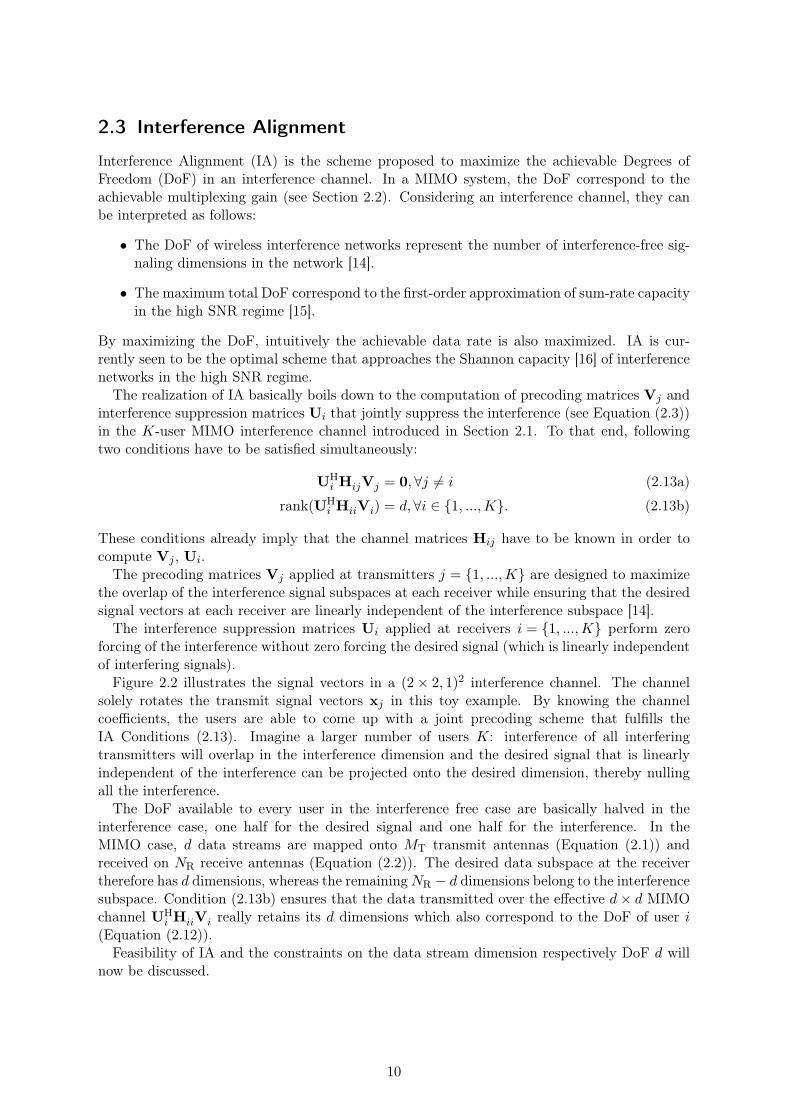
Figure 2.2 illustrates the signal vectors in a (2× 2, 1)2 interference channel. The channelsolely rotates the transmit signal vectors xj in this toy example. By knowing the channelcoefficients, the users are able to come up with a joint precoding scheme that fulfills theIA Conditions (2.13). Imagine a larger number of users K: interference of all interferingtransmitters will overlap in the interference dimension and the desired signal that is linearlyindependent of the interference can be projected onto the desired dimension, thereby nullingall the interference.

The DoF available to every user in the interference free case are basically halved in theinterference case, one half for the desired signal and one half for the interference. In theMIMO case, d data streams are mapped onto MT transmit antennas (Equation (2.1)) andreceived on NR receive antennas (Equation (2.2)). The desired data subspace at the receivertherefore has d dimensions, whereas the remaining NR − d dimensions belong to the interferencesubspace. Condition (2.13b) ensures that the data transmitted over the effective d× d MIMOchannel UH

i HiiVi really retains its d dimensions which also correspond to the DoF of user i(Equation (2.12)).

Feasibility of IA and the constraints on the data stream dimension respectively DoF d willnow be discussed.

10

inte

rfer

ence

desired

desired

inte

rfer

ence

TX1 RX1

RX2TX2

Figure 2.2: Signal vectors in a (2× 2, 1)2 interference channel without noise

2.3.1 Feasibility

Feasibility of IA in general was researched in [14] whereas the MIMO symmetric square casewas researched in [17]. In [14], IA was found to be (almost surely) feasible if a system isproper. A system is said to be proper if the number of variables is not smaller than thenumber of equations in Condition (2.13a) (non-overdetermined system of linear equations). Ina symmetric (MT ×NR, d)

K system, this boils down to following condition [14]:

MT +NR − (K + 1)d ≥ 0. (2.14)

Assuming equal number of transmit and receive antennas MT = NR (symmetric square case)and generic channel matrices (non-degenerate continuously distributed entries), IA is feasibleif and only if [17]

NR ≥ d(K + 1)

2. (2.15)

Furthermore, for K ≥ 3 and generic channel matrices, the maximum number of total DoF isgiven as [17]

DoFmax =K

NR

⌊2NR

K + 1

⌋≤ 2

K

K + 1. (2.16)

The symmetric square case with MT = NR = 4 antennas at each node and K = 3 users asinvestigated in this work attains the maximum DoF achievable in a 3-user system:

DoFmax =3

4

⌊2 · 43 + 1

⌋

︸ ︷︷ ︸= 3

2

= 23

3 + 1︸ ︷︷ ︸= 3

2

. (2.17)

11

2.3.2 Closed Form Solution

The computation of a closed form analytical solution for the IA precoding matrices Vj andinterference suppression matrices Ui for the symmetric K = 3-user MIMO square case is nowelaborated, following [5]. The conditions imposed on these matrices have already been definedin Equation (2.13). The truncated unitary interference suppression matrix Ui describes anorthonormal basis for the interference free subspace at the ith receiver. The receive signalvector is projected onto this interference free subspace as stated in Equation (2.3). To performsuppression, the received interference must lie in the NR − d dimensional nullspace of UH

i andhence

span(HijVj

)⊆ null

(UH

i

), ∀i 6= j, (2.18)

which is basically a reformulation of Condition (2.13a), giving more insight into the nature ofthe problem. To satisfy Conditions (2.13) and Condition (2.18), the precoding matrices mightbe computed as follows:

V2 = ν(H−1

32 H31H−121 H23H

−113 H12

), (2.19a)

V1 = H−121 H23H

−113 H12V2, (2.19b)

V3 = H−113 H12V2, (2.19c)

where ν(.) arbitrarily chooses d eigenvectors to compose V2. This solution is clearly not uniquedue to the arbitrary choice of eigenvectors in Equation (2.19a) and due to the fact that anyrotation inside its subspace yields another valid solution.

The corresponding interference suppression matrices are then obtained as:

U1 = ν left (H12V2) , (2.20a)

U2 = ν left (H21V1) , (2.20b)

U3 = ν left (H32V2) , (2.20c)

where ν left(.) arbitrarily chooses NR − d left singular vectors6.

The IA solution described above does not maximize the sum rate directly as it solely focuseson nulling the interference and hence maximizing the SIR at the receiver to infinity. Perfectalignment may even reduce the SNR as a result of projecting the receive signal vector ontothe interference free subspace (see toy example in Figure 2.2). Improved iterative solutionswith constraints on maximizing the Signal to Interference and Noise Ratio (SINR) have beenproposed in [3, 5].

This work predominantly focuses on showing the feasibility of IA, online on a testbed. Theclosed form solutions presented above are hence sufficient (and efficient to compute).

6Let A = LΣRH denote the singular value decomposition of A. The columns of L are called left singularvectors of A.

12

Chapter 3

Vienna MIMO Testbed

Section 3.1 gives a hardware overview of the Vienna MIMO Testbed (VMTB), and a link tothe theoretical discourse in Section 2.1 is drawn. Section 3.2 subsumes the procedures of ameasurement cycle. In Section 3.3, the used signals to perform IA measurements are explainedin detail and channel estimation is described. Finally, Section 3.4 focuses on the underlyingsoftware implementation performing the various measurements and provides understandingover the sequential chain of events.

3.1 Hardware and Deployment

The VMTB in the setup considered here1 consists of two outdoor transmitter stations TX1 andTX2 located on rooftops, one indoor transmitter station TX3 and one indoor receiver stationRX. Both indoor stations are located on the 5th floor of the Institute of Telecommunicationsat Vienna University of Technology and are within Line of Sight (LOS) of each other. Thisheterogeneous2 setup represents an urban scenario. The deployment of all stations is depictedin Figure 3.1.

© 2013 GoogleTX2

TX1

160m

140m

RXTX3

Figure 3.1: Deployment of Vienna MIMO Testbed

1Contrary to the description in [18], transmitter station TX3 was located indoors throughout this work.2A heterogeneous scenario in this context contains outdoor to indoor and indoor to indoor radio links.

13

antenna GPS

RX location

Figure 3.2: TX1 antenna setup

antenna humidityprecipitation windGPS

Figure 3.3: TX2 antenna setup with sensors

antennas TX3

Figure 3.4: TX3 station

TX3 antenna setup RX antenna setup

Figure 3.5: TX3 to RX indoor channel

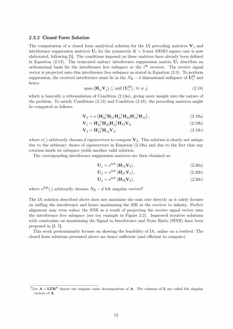
Each station comprises a Personal Computer (PC), RF hardware, synchronization hardwareand an antenna setup with 4 antennas. Figure 3.2 and Figure 3.3 show the antenna setup oftransmitter TX1 and TX2, respectively. The antenna setup of TX2 employs a variety of sensorsto monitor the environmental conditions. Figure 3.4 shows the indoor transmitter station ofTX3, Figure 3.5 depicts the indoor LOS channel from TX3 to RX. All PCs are connected viaa dedicated fiber network to communicate with each other.

Comparing this setup to the K = 3-user interference channel depicted in Figure 2.1, theabsence of two receivers is recognized. RX is chosen as counterpart of the desired transmit-ter, selectable from j ∈ {1, 2, 3}. The resulting desired link is denoted as I ∈ {1, 2, 3}, wherei = j = I on the desired link. For example, the desired transmitter shall be TX1 (j = 1).The corresponding receiver therefore is RX1 (i = 1). The desired link is I = 1, and RX playsthe role of RX1. Channels to the remaining two receivers are chosen randomly as defined inSection 3.3.3 to compensate for their absence.

14

3.1.1 Transmitter

The transmit-hardware included in all three transmitter stations (TX1, TX2 and TX3) is nowcharacterized, subsuming the detailed description in [19]. Figure 3.6 shows the basic structureof a transmitter.

transmitter PC

transmitter

daemon

X5-TX

module

MATLABDRAM

flash

storage

testbed

attenuatorupconverter

bandpass

filter

power

amplifier

4 x RF

frequency

standard

timing unit

GPS

module

1 PPS10 MHz

2.433 GHz

4 x 70 MHz IF

4 x 2.503 GHz

200 MHz

trigger

clock

internal

LAN

external

LAN

Figure 3.6: Transmitter overview [19]

• Transmitter PC: Contains an INNOVATIVE INTEGRATION X5-TX FIFO Digital toAnalog Conversion (DAC) card that generates transmit samples at 70MHz IntermediateFrequency (IF). The X5-TX card includes four channels, works at sampling frequency200MHz and has a resolution of 16 bit. For the measurements in this work, an efficientC++3 transmit routine was developed (see Section 3.4.2) that generates the IF samplesand stores them directly in the DRAM4 which results in high transmission rates. Al-ternatively, the transmit samples can be stored on a flash storage device embodied bya SSD5. A MATLAB6 daemon that is responsible for start-up and initialization tasksprior to measurements is running on each transmitter PC. All PCs are connected via adedicated fiber network (LAN7). The transmit routine is invoked via LAN.

• RF Hardware: The RF chain contains an upconverter that filters the 70MHz IF fromthe X5-TX module and converts it up to 2.503GHz transmit frequency. The bandpassfilter has a bandwidth of 20MHz. The maximum output power of the chain is 35 dBmand can be attenuated by an AEROFLEX 4226 digitally programmable attenuator thatallows attenuations from 0 dB to 63 dB with 1 dB step size. These attenuators will beused to control the transmit power of each transmitter individually.

3C++ is an object oriented compiled programming language.4DRAM... Dynamic Random Access Memory5SSD... Solid State Drive6MATLAB is a numerical computing environment and programming language developed by MathWorks.7LAN... Local Area Network

15

• Synchronization Hardware: A common timebase for the whole testbed is derivedfrom a TRIMBLE Acutime GPS8 module. The so obtained PPS9 signal is used bya STANFORD RESEARCH SYSTEM Rubidium FS725 frequency standard to outputa precise 10MHz reference for the oscillators depicted in Figure 3.6. The reference isthereby used to generate the clock for the local oscillator used for upconversion, theX5-TX card and the timing unit. The timing unit responsible for synchronization andtriggering the X5-TX module is described in [20].

• Antenna Setup: Whereas the transmit hardware described previously is built on awooden desk mounted on wheels, the antennas might be located elsewhere (still connectedwith cables). In case of TX1 and TX2, they are outdoors on rooftops as illustrated inFigure 3.2 and Figure 3.3. Every setup comprises MT = 4 antennas. The used antennatypes are now listed:

TX1,TX2: KATHREIN Scala Division 60◦ XX-pol panel antenna (800 10543)

TX3: 2 × KATHREIN Scala Division X-pol directional indoor antenna (800 10677)

3.1.2 Receiver

An overview of the receive hardware of RX is now provided, summarizing the detailed work of[21]. Figure 3.7 shows the basic structure of the receiver.

radio frequency

front end ADC

PCIe CardRAM

daemon

Matlab

script

receiver PC

timing

unit

internal

LAN

HDD

10 MHz

2.433 GHz

rubidium

200 MHz

2.503 GHz 70 MHz

oscillator+

splitter

Figure 3.7: Receiver overview [21]

• Receiver PC: Contains an INNOVATIVE INTEGRATION X5-RX FIFO Analog toDigital Conversion (ADC) card that fetches the receive samples at 70MHz IF. Similarto the X5-TX card, it includes four channels, works at sampling frequency 200MHz andhas a resolution of 16 bit. The receive samples are stored on a RAMDrive10 which allowsfast processing. RX is also the control node in the system. Measurement script (seeSection 3.4.1) and thus transmissions are invoked from here.

8GPS... Global Positioning System9PPS... Pulse Per Second

10RAMDrive is a virtually generated drive in the random access memory that entails higher reading and writingspeeds than conventional hard disk drives.

16

• RF Hardware: The radio frequency front end receives the signal at center frequency2.503GHz and includes several filtering operations, downconversion to 70MHz IF andamplification before the signal is fed into the X5-RX card.

• Synchronization Hardware: Essentially the same function as at the transmitters -see Section 3.1.1.

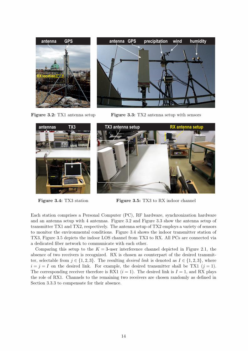
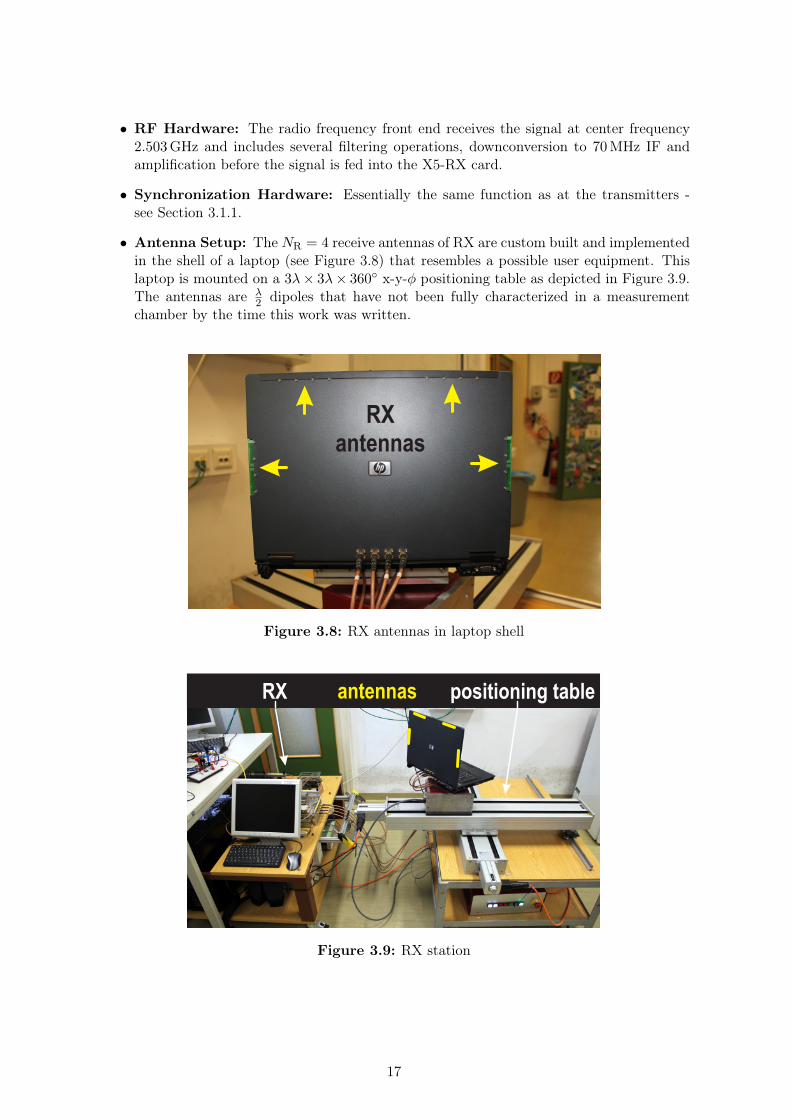
• Antenna Setup: The NR = 4 receive antennas of RX are custom built and implementedin the shell of a laptop (see Figure 3.8) that resembles a possible user equipment. Thislaptop is mounted on a 3λ× 3λ× 360◦ x-y-φ positioning table as depicted in Figure 3.9.The antennas are λ

2 dipoles that have not been fully characterized in a measurementchamber by the time this work was written.

RXantennas

Figure 3.8: RX antennas in laptop shell

antennas positioning tableRX

Figure 3.9: RX station

17

3.2 Measurement Methodology

A measurement cycle entails successive frame transmissions. Each frame contains a pilot pream-ble and data. Let the frames (and hence transmissions) be indexed by l. The pilot preamble of

frame (l) is used to compute the estimated channel matrices H(l)Ij , where I denotes the desired

link and j ∈ {1, 2, 3} the used transmitters. The estimated channel matrices are used to com-

pute the precoding matrices V(l)j and interference suppression matrices U

(l)i . These are then

applied on the data of frame (l + 1). The process is illustrated in Figure 3.10. IA as used herehence requires constant channels to work perfectly, a requirement that will not be met in thereal world. However, by keeping the processing time Tp between two consecutive frames as lowas possible, the channels in a quasi-static setup hardly change (the filters Ui and Vj computedfrom frame (l) are suitable but not ideal for the channel realization at frame (l + 1)).

Computation of channel estimates, precoding matrices and interference suppression matricestakes place online. The evaluation and validation of IA takes place offline.

Figure 3.10: Two consecutive transmit frames

3.3 Signals and Channel Estimation

Orthogonal Frequency Division Multiplexing (OFDM) is used as modulation format. Thecomputational complexity increases with the number of subcarriers, since channel estimationand precoder computation has to be performed on each subcarrier individually. To ensure fastprocessing times between frames (see Figure 3.10), only one subcarrier is used in this work.This is sufficient to show the feasibility of IA. Furthermore, no subcarrier indexation is neededin the description. The general signal specifications are listed in Table 3.1.

parameter value

sampling rate 200MHz

oversampling factor 13

subcarrier spacing 15.02 kHz

FFT length 1024

symbol duration 66.56 µs

cyclic prefix duration 4.94 µs

signal constellation 4QAM

Table 3.1: Signal specifications

18

3.3.1 Transmit Signals

The generation of an OFDM transmit symbol from symbol level to Intermediate Frequency (IF)samples is now discussed. First, the single antenna case with no precoding matrix is explained.The transmit symbols of one OFDM symbol are defined in frequency domain. Up to C = 1024(number of subcarriers) symbols are accommodated in one OFDM symbol. Let c denote thesubcarrier index and k the sample index (time). In general, the baseband samples xBB[k] ofone OFDM symbol are obtained by a C-point Inverse Fast Fourier Transform (IFFT) appliedon the symbols in frequency domain S[c]:

xBB[k] =1

C

C−1∑

c=0

S[c] exp

(j2π

tc

C

), 0 ≤ k < C. (3.1)

This work restricts itself to only one subcarrier, namely the DC subcarrier at 0Hz. The corre-sponding symbol is S = S[0], the other symbols are zero. Considering this in Equation (3.1),the resulting baseband samples of one OFDM symbol will just be a repetition of the scaledfrequency domain symbol:

xBB[k] =1

CS, 0 ≤ k < C. (3.2)

The cyclic prefix is attached by inserting a copy of the last NCP = 72 samples before the OFDMsymbol. One OFDM symbol contains C = 1024 samples, its duration11 is 1024 · 5 ns = 5.12 µs.To increase the duration to 66.56 µs, upsampling with factor 13 is performed by repeating eachsample 13 times. The resulting signal is then upconverted to 70MHz IF. Furthermore, scalingfactors are introduced. The IF transmit samples are:

xIF[k] = C√2︸ ︷︷ ︸

scaling

Re

1

CS exp

(j2π

70

200k

)

︸ ︷︷ ︸upconversion

=√2Re

{S exp

(j2π

70

200k

)}

=1√2

(S exp

(j2π

70

200k

)+ S∗ exp

(−j2π

70

200k

)), 0 ≤ k < 13(NCP + C).

(3.3)

Since the the X5-TX FIFO DAC card requires 16 bit integer values, samples are scaled with aDAC scaling factor and converted from floating point to integer values:

xIF[k] =⌊DACscaling · xIF[k]

⌋, 0 ≤ k < 13(NCP + C). (3.4)

These are the final OFDM symbol samples that are ready to be written into memory for trans-mission.

Advancing to the multiple antenna case with precoding matrix, the symbols are stored in avector

s[c] =

S0[c]

S1[c]...

Sd−1[c]

, (3.5)

11Sampling frequency of the DAC/ADC cards is fixed at 200MHz.

19

where d denotes the number of data streams. The precoding matrix V ∈ CMT×d is applied at

symbol level. The baseband samples xBB[k] ∈ CMT of an OFDM symbol are generally obtained

by applying a C-point IFFT on the elements of the symbol vector s[c] as

xBB[k] =1

C

C−1∑

c=0

V[c]s[c] exp

(j2π

tc

C

), 0 ≤ k < C. (3.6)

Utilizing only the DC subcarrier c = 0 and following the same steps as before, the transmitsignal vector at 70MHz IF xIF[k] ∈ R

MT becomes

xIF[k] =√2Re

{Vs exp

(j2πk

70

200

)}, 0 ≤ k < 13(NCP + C). (3.7)

Finally, conversion to integer values is performed:

xIF[k] =⌊DACscaling · xIF[k]

⌋, 0 ≤ k < 13(NCP + C). (3.8)

These are the final OFDM symbol samples xIF[k] ∈ NMT

0+ that are ready to be written intomemory for transmission. MT = 4 channels are utilized on the VMTB.

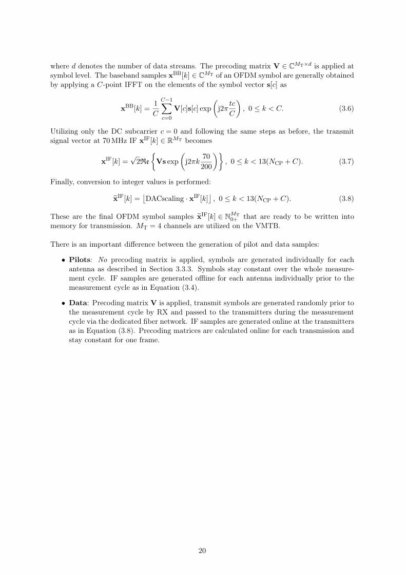
There is an important difference between the generation of pilot and data samples:

• Pilots: No precoding matrix is applied, symbols are generated individually for eachantenna as described in Section 3.3.3. Symbols stay constant over the whole measure-ment cycle. IF samples are generated offline for each antenna individually prior to themeasurement cycle as in Equation (3.4).

• Data: Precoding matrix V is applied, transmit symbols are generated randomly prior tothe measurement cycle by RX and passed to the transmitters during the measurementcycle via the dedicated fiber network. IF samples are generated online at the transmittersas in Equation (3.8). Precoding matrices are calculated online for each transmission andstay constant for one frame.

20

3.3.2 Receive Signals

First, the interference free single antenna case is discussed. The transmit signal from Equa-tion (3.4) is transmitted over a linear time-invariant channel with baseband impulse responseh[k] of length L samples:

yIF[k] =⌊hIF[k] ∗ xIF[k]

⌋, (3.9)

where hIF[k] = 2Re(h[k] exp

(j2π 70

200k))

is the equivalent IF impulse response. The error dueto quantization at the receiver is modeled as noise which will be omitted in the followingdescription. The 16 bit integer receive samples at 70MHz IF yIF[k] ∈ N0+ of one time dispersedOFDM symbol (cyclic prefix discarded) are read out from RAMDrive and converted back tofloating point values

yIF[k] =1

DACscaling· yIF[k],

⌈L

2

⌉+ 13NCP − 1 ≤ k < 13(NCP + C) +

⌈L

2

⌉− 2. (3.10)

Scaling and downconversion is then performed on the OFDM symbol samples according to:

yBB,US[k] =

√2

C︸︷︷︸scaling

yIF[k] exp

(−j2πk

70

200

)

︸ ︷︷ ︸downconversion

=

√2

C

(hIF[k] ∗ xIF[k]

)exp

(−j2πk

70

200

)

= h[k] ∗ xBB,US[k] +(h[k] ∗ xBB,US[k]

)∗exp

(−j2πk

2 · 70200

),

⌈L

2

⌉+ 13NCP − 1 ≤ k < 13(NCP + C) +

⌈L

2

⌉− 2.

(3.11)

The baseband OFDM symbol is then downsampled by factor 13. This is done by retainingonly every 13th sample in the upsampled baseband symbol samples yBB,US[k] and applying alowpass filter that suppresses the frequency component at −140MHz. A C-point Fast FourierTransform (FFT) is applied and the received symbols in frequency domain are:

R[c] =C−1∑

k=0

y[k]BB exp

(−j2π

ct

C

), 0 ≤ c < C. (3.12)

Since only the DC subcarrier c = 0 was utilized in the transmission, the received symbol is

R = R[0] = H[0]S[0], (3.13)

where H[c] is the Fourier transform of the downsampled and filtered impulse response. Dueto the usage of a cyclic prefix with NCP ≥ L, no inter-symbol interference occurs if more thanone OFDM symbol is transmitted.

Advancing to the multiple antenna case with interference, a vector of sample instances at70MHz IF yIF[k] ∈ N

N0+ is received whose elements are obtained as

yIFn [k] =

⌊KMT−1∑

m=0

hIFnm[k] ∗ xIF

m [k]

⌋, (3.14)

where m denotes the transmit antenna index, n the receive antenna index, hIFnm[k] the channel

impulse response between two antennas at IF and the total number of transmit antennas is

21

obtained as KMT since the system as in Figure 2.1 has K transmitters with MT antennaseach. The elements of yIF[k] are then converted to floating point values the same way as inEquation 3.10. Scaling, downconversion, downsampling and filtering is performed.

Equivalently to the transmit signals, there is a difference in the receive sample processing ofpilots and data:

• Pilots: No interference suppression matrix is applied, receive symbols at each antennaare stacked in a vector r = [R0, R1, ..., RNR−1]

T which is obtained as

r = Hs+ n. (3.15)

• Data: Interference suppression matrix U ∈ CNR×d is applied, receive symbols at each

data stream are stacked in a vector r = [R0, R1, ..., Rd−1]T which is obtained as

r = UHHVs+UHn. (3.16)

This formulation is equivalent to the interference channel formulation in Equation (2.3).

The overall channel matrix H ∈ CNR×KMT contains the complex valued channel coefficients

(H)nm from transmit antenna m to receive antenna n. In the case of K = 3 transmitters:

r = rI ,

U = UI ,

H =[HI1 HI2 HI3

],

V =

V1

V2

V3

,

s =

s1

s2

s3

,

n = nI ,

(3.17)

where I denotes the desired link index.

22

3.3.3 Channel Estimation

Channel coefficients (H)nm from every transmit antenna m = {0, ...,KMT − 1} to every receiveantenna n = {0, ..., NR − 1} are estimated. The channel is assumed to stay constant duringone frame. A pilot preamble in every frame contains pilot symbols for channel estimation, seeFigure 3.10. Note that in the following, t denotes the OFDM symbol index (time). Orthogonalsymbol sequences optimal for multiple antenna systems are used as proposed in [22]. Thesequence length depends on the number of transmit antennas. The length 16 QPSK sequence

SP = {1, 1, 1, 1, 1, j,−1,−j, 1,−1, 1,−1, 1,−j,−1, j}is used, it is circularly shifted by one symbol for each transmit antenna m:

SPm[t] = SP[(t+m) mod 16]. (3.18)

The sequence is orthogonal to circularly shifted instances of itself, the cyclic autocorrelationfunction ρ[q] has zero off peaks:

ρSP [q] =1

16

15∑

t=0

SP[t mod 16] ·(SP[(t− q) mod 16]

)∗= δ[q]. (3.19)

Therefore, up to 16 orthogonal sequences can be generated from SP and up to 16 transmitantennas are supported.

Channel Estimation is performed at receiver I ∈ {1, 2, 3} via cross-correlation of the receivesymbol sequence Rn[t] with the known transmit symbol sequence SP

m[t] (Equation (3.18)).Assuming perfect synchronization so that the pilot sequences are received at the same time,the channel coefficient from transmit antenna m to receive antenna n is obtained as

(H)nm = ρRn,SPm[0] =

=1

16

15∑

t=0

(KMT−1∑

m′=0

(H)nm′SPm′ [t] + nn[t]

)

︸ ︷︷ ︸Rn[t]

·(SPm[t]

)∗

= (H)nm1

16

15∑

t=0

SPm[t] ·

(SPm[t]

)∗

︸ ︷︷ ︸=1

+

KMT−1∑

m′=0m′ 6=m

(H)nm′

1

16

15∑

t=0

SPm′ [t] ·

(SPm[t]

)∗

︸ ︷︷ ︸=0

+1

16

15∑

t=0

nn[t] ·(SPm[t]

)∗

︸ ︷︷ ︸=nn

= (H)nm + nn.

(3.20)

The estimated matrix contains the estimated channel matrices from all transmitters j ∈ {1, 2, 3}to desired receiver I,

H =[HI1 HI2 HI3

]. (3.21)

The remaining channel matrices, called virtual channel matrices, are generated randomly as(full rank) complex Gaussian matrices:

Hij ∼ CN (0, IMT), i ∈ {1, 2, 3} ∧ i 6= I, j ∈ {1, 2, 3}. (3.22)

They are generated prior to a measurement cycle and stay constant for the whole cycle.

23

3.4 Software and Control

3.4.1 Measurement

The MATLAB measurement script is now explained in detail. The sequence of events isillustrated in Figure 3.13. The description focuses on the main flow of the script rather thanexplaining every function in detail. The step numbers coincide with the sequence numbers inFigure 3.13.

1. The name of the measurement is defined, for example dummy. The default paths are thengenerated as follows:

pathTX: D:\hiatus\ ...local on the TX PCs

pathRX: G:\hiatus\ ...local on the RX PC, this is the RAMDrive

pathMeasurement: S:\30_HIATUS\Measurements\dummy\ ...on testbed server

2. Settings are loaded. To that end, the loadSettings(’settings’) function is executed.It contains predefined settings for the measurement selected by the parameter string’settings’.

3. Pilot symbols are generated according to ’settings’. Then, OFDM symbol samples arecreated (see Section 3.3.1 for details). The parametersettings.OFDMTrainingSequence contains the used pilot sequence. Default value is:settings.OFDMTrainingSequence = TrainingSequence16.This is a 4QAM sequence that is orthogonal to circularly shifted versions of itself (finddetails in Section 3.3.3). It supports channel estimation with up to 16 transmit antennas.TrainingSequence16 = [1,1,1,1,1,1i,-1,-1i,1,-1,1,-1,1,-1i,-1,1i]

4. Data symbols for all transmissions are generated according to ’settings’. Since 4QAMsymbols entail a finite alphabet, it suffices to store the symbol indices as depicted inTable 3.2. “Zero symbols” (0) are also possible. For each transmission, the data symbolindices are sent to the respective transmitters via the fiber network included in an UDP12

message.

symbol index

0 0

1 + j 1

−1 + j 2

−1− j 3

1− j 4

Table 3.2: Transmit symbol indices of 4QAM alphabet

5. Initial transmit signal samples are created. Figure 3.11 shows the basic composition of atransmit signal. The zero padding is used for transmitter synchronization (see step 7) and

12UDP... User Datagram Protocol

24

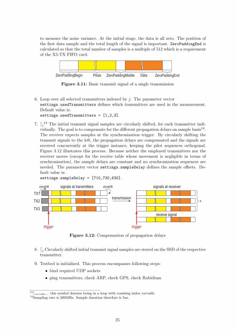
to measure the noise variance. At the initial stage, the data is all zero. The position ofthe first data sample and the total length of the signal is important. ZeroPaddingEnd iscalculated so that the total number of samples is a multiple of 512 which is a requirementof the X5-TX FIFO card.

ZeroPaddingBegin ZeroPaddingMiddle ZeroPaddingEndPilots Data

Figure 3.11: Basic transmit signal of a single transmission

6. Loop over all selected transmitters indexed by j. The parameter vectorsettings.usedTransmitters defines which transmitters are used in the measurement.Default value is:settings.usedTransmitters = [1,2,3].

7. ⌈j13 The initial transmit signal samples are circularly shifted, for each transmitter indi-vidually. The goal is to compensate for the different propagation delays on sample basis14.The receiver expects samples at the synchronization trigger. By circularly shifting thetransmit signals to the left, the propagation delays are compensated and the signals arereceived concurrently at the trigger instance, keeping the pilot sequences orthogonal.Figure 3.12 illustrates this process. Because neither the employed transmitters nor thereceiver moves (except for the receive table whose movement is negligible in terms ofsynchronization), the sample delays are constant and no synchronization sequences areneeded. The parameter vector settings.sampleDelay defines the sample offsets. De-fault value is:settings.sampleDelay = [710,730,630].

trigger trigger

TX1

TX2

TX3

signals at transmitters signals at receiver

receive signal

+transmission

circshift circshift

Figure 3.12: Compensation of propagation delays

8. ⌈j Circularly shifted initial transmit signal samples are stored on the SSD of the respectivetransmitter.

9. Testbed is initialized. This process encompasses following steps:

• bind required UDP sockets

• ping transmitters, check ARP, check GPS, check Rubidium

13⌈variable... this symbol denotes being in a loop with counting index variable14Sampling rate is 200MHz. Sample duration therefore is 5ns.

25

• calibrate DACs

• initialize synchronization units

10. Initial UDP message is created. It is intended to pass initial information to the trans-mitters, such as:

• pathTX: Tells the transmitters where the initial data is stored.

• data sample offset: Tells the transmitters where the data samples begin in thetotal transmit signal. This is important later on because the transmit routine thatgenerates the data samples online has to know where to write them into the memory.

• DAC scaling: The DAC works with 16 bit integer values (all samples that are loadedinto the X5-TX FIFO card memory have to be in that format). The transmit signalsamples have to be converted from floating point to 16 bit integer according toEquation (3.4). Default value is:settings.DACscaling = 214.3/settings.numTxAntennasTotal.

11. Loop over all selected transmitters indexed by j.

12. ⌈j Initial UDP message created in step 10 is sent to the transmitters via dedicated fibernetwork.

13. The channel estimation operator matrix Z is generated. Channel estimation (see Sec-tion 3.3.3 for details) is thereby reduced to a multiplication of the pilot receive samplesyp with the estimation operator matrix:

H =[HI1 HI2 HI3

]= ypZ.

14. Virtual channel matrices for the non-existing receivers are generated according to Equa-tion (3.22).

15. Loop over transmissions indexed by l. One measurement cycle entailssettings.numTransmissions transmissions.

16. ⌈l Loop over transmitters indexed by j.

17. ⌈l ⌈j Generate transmit UDP message for each transmitter individually. The messagecontains:

• precoders: these are the precoding matrices Vj

• data symbols: 4QAM symbol indices as generated in step 4

• attenuator info: 6 bit hardware attenuator value

18. ⌈l ⌈j Send transmit UDP message. The respective transmitter then executes the C++transmit routine to generate the transmit data samples (see Section 3.4.2).

19. ⌈l While the transmitters are generating the samples and store them in the memory oftheir X5-TX FIFO card, the receiver RX is waiting.

20. ⌈l Transmission is triggered and samples are received and stored on the RAMDrive ofRX.

26

21. ⌈l When transmission is over and receiver is ready, the pilot samples are read out fromthe RAMDrive. The remaining signal samples, namely data and noise samples, are usedin the offline evaluation.

22. ⌈l Channel estimation is performed according to step 13.

23. ⌈l The precoders Vj and interference suppression matrices Ui are calculated with theclosed form solution defined in Section 2.3.2.

24. ⌈l Optional: table is repositioned.

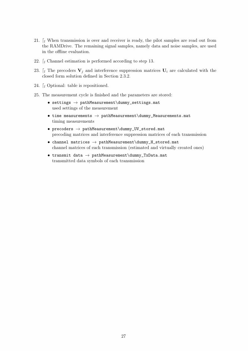
25. The measurement cycle is finished and the parameters are stored:

• settings → pathMeasurement\dummy_settings.mat

used settings of the measurement

• time measurements → pathMeasurement\dummy_Measurements.mat

timing measurements

• precoders → pathMeasurement\dummy_UV_stored.mat

precoding matrices and interference suppression matrices of each transmission

• channel matrices → pathMeasurement\dummy_H_stored.mat

channel matrices of each transmission (estimated and virtually created ones)

• transmit data → pathMeasurement\dummy_TxData.mat

transmitted data symbols of each transmission

27

load settings

generate pilot symbols and samples

generate initial TX signal samples

store initial TX signal samples

circularly shift TX samples (sample delay)

testbed initialization

generate init UDP message[pathTX, data sample offset, DAC scaling]

generate virtual channel matrices

generate channel estimation operator matrix

send TX UDP message to transmitter

wait for reception

store receive samples in file

read out pilot samples

perform channel estimation

calculate precoders

optional: move table

save measurement parameters:settings, time measurements, precoders,channel matrices, transmit data

send init UDP message to transmitter apply initializations

execute transmit routine and generate samples

store samples in memory

transmit (synchronized transmitters)

load initial TX signal samples into memory

generate TX UDP message[precoders, data symbols, attenuator info]

generate data symbols

define measurement name and paths

RX TX1, TX2, TX3

pathTX

pathRX

pathRX

pathMeasurement

pathTX

fiber

fiber

local

LAN

fiber

radioRAMDrive RX

SSD TX1...3

SSD TX1...3

\\tbsrv1.nt.tuwien.ac.at

local

local

loop over transmitters

loop over transmitters

1

2

3

4

5

6

7

8

9

10

11

12

13

14

15

17

18

19

20

21

22

23

24

25

fiber... dedicated fiber LAN for testbed... radio transmission link over antennasradio

... local on PClocal

... institute LANLAN

loop over transmitters 16

loop over transmissions

Fig

ure

3.1

3:

Measu

remen

tscrip

t

28

3.4.2 Transmit Routine

For each frame, the C++ transmit routine newly generates data samples out of the numberencoded data symbols that are passed from RX to the transmitters. This has to be done inan efficient manner to keep the processing time Tp between frame transmissions low. To thatend, Equation (3.3) is studied and following aspects lead to an efficient implementation:

• Equation (3.3) can further be decomposed:

xIF[k] =√2Srecos

(2π

70

200k

)−√2Simsin

(2π

70

200k

), 0 ≤ k < 13(NCP + C),

where Sre and Sim denote the real and imaginary part of symbol S, respectively.

• The upconversion multipliers cos(2π 70

200k)

and sin(2π 70

200k)

have a periodicity of 20 sam-ples. Two tables, each containing 20 values, can be computed in advance.

• The baseband samples of one OFDM symbol are constant because only the DC subcarrieris used (see Equation (3.2)). Therefore, the OFDM symbol samples are just a repetitionof the upconversion table values multiplied with the symbol value.

• Cyclic prefix length NCP is chosen in order to make the total number of samples of theOFDM symbol including cyclic prefix a multiple of 20:

13(NCP + C) mod 20 = 0.

This way, concatenation of OFDM symbols does not lead to phase jumps in the upcon-version multipliers.

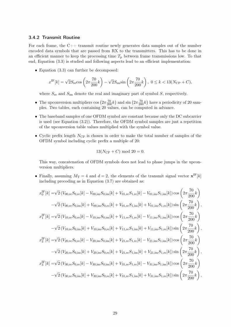
• Finally, assuming MT = 4 and d = 2, the elements of the transmit signal vector xIF[k]including precoding as in Equation (3.7) are obtained as:

xIF0 [k] =

√2 (V00,reS0,re[k]− V00,imS0,im[k] + V01,reS1,re[k]− V01,imS1,im[k]) cos

(2π

70

200k

)

−√2 (V00,reS0,im[k] + V00,imS0,re[k] + V01,reS1,im[k] + V01,imS1,re[k]) sin

(2π

70

200k

),

xIF1 [k] =

√2 (V10,reS0,re[k]− V10,imS0,im[k] + V11,reS1,re[k]− V11,imS1,im[k]) cos

(2π

70

200k

)

−√2 (V10,reS0,im[k] + V10,imS0,re[k] + V11,reS1,im[k] + V11,imS1,re[k]) sin

(2π

70

200k

),

xIF2 [k] =

√2 (V20,reS0,re[k]− V20,imS0,im[k] + V21,reS1,re[k]− V21,imS1,im[k]) cos

(2π

70

200k

)

−√2 (V20,reS0,im[k] + V20,imS0,re[k] + V21,reS1,im[k] + V21,imS1,re[k]) sin

(2π

70

200k

),

xIF3 [k] =

√2 (V30,reS0,re[k]− V30,imS0,im[k] + V31,reS1,re[k]− V31,imS1,im[k]) cos

(2π

70

200k

)

−√2 (V30,reS0,im[k] + V30,imS0,re[k] + V31,reS1,im[k] + V31,imS1,re[k]) sin

(2π

70

200k

),

29

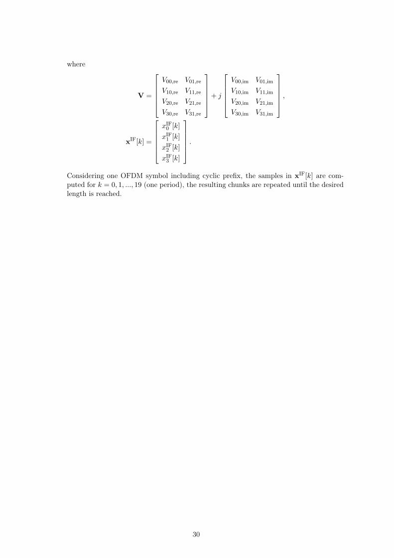
where

V =

V00,re V01,re

V10,re V11,re

V20,re V21,re

V30,re V31,re

+ j

V00,im V01,im

V10,im V11,im

V20,im V21,im

V30,im V31,im

,

xIF[k] =

xIF0 [k]

xIF1 [k]

xIF2 [k]

xIF3 [k]

.

Considering one OFDM symbol including cyclic prefix, the samples in xIF[k] are com-puted for k = 0, 1, ..., 19 (one period), the resulting chunks are repeated until the desiredlength is reached.

30

Chapter 4

Evaluation and Quantities of Interest

This section introduces performance measures to evaluate the measurements. Evaluation takesplace offline after the measurement and utilizes the stored receive samples. Section 4.1 dis-cusses assumptions on the involved signals and explains the detailed frame structure. Datacovariance matrices are introduced. Section 4.2 then describes two different means to computethe mutual information. Section 4.3 introduces a measure for interference suppression andfinally, Section 4.4 defines measured powers, SNR and SIR.

4.1 Assumptions and Detailed Frame Structure

Based upon the K = 3-user MIMO interference channel model introduced in Section 2.1, detailsregarding signals and noise as encountered on the VMTB are now discussed.

Analogous to Equation (2.3), the receive signal vector at RX decomposes into three compo-nents:

yI =K∑

j=1

HIjVjsj + nI = HIIVIsI︸ ︷︷ ︸desired signal

+K∑

j=1j 6=I

HIjVjsj

︸ ︷︷ ︸interference

+ nI︸︷︷︸noise

. (4.1)

These components can be summarized as follows:

• desired signal: signal of interest from desired transmitter TXI, I ∈ {1, 2, 3} denotesthe desired link index

• interference: signals from interfering transmitters TXj, j ∈ {1, 2, 3} ∧ j 6= I

• noise: additive noise at RX

All three components are assumed to be statistically independent. The transmit data streamssj ∈ Sd contain 4QAM symbols picked from the symbol alphabet

S = {S(1), S(2), S(3), S(4)} =1√2{1 + j,−1 + j,−1− j, 1− j}.

The transmit symbols are equally likely and hence uniformly distributed:

P{S(1)} = P{S(2)} = P{S(3)} = P{S(4)} =1

4.

The additive Gaussian noise is not spatially white as assumed in Section 2.1 and is generallydistributed according to nI ∼ CN (0,QnI

), where QnI∈ C

NR×NR denotes the noise covariancematrix.

31

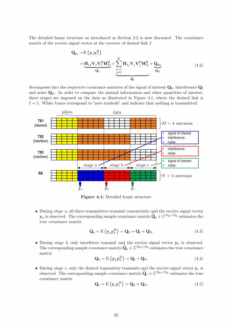
The detailed frame structure as introduced in Section 3.2 is now discussed. The covariancematrix of the receive signal vector at the receiver of desired link I

QyI=E

{yIy

HI

}

=HIIVIVHI H

HII︸ ︷︷ ︸

QS

+K∑

j=1j 6=I

HIjVjVHj H

HIj

︸ ︷︷ ︸QI

+QnI︸︷︷︸QN

(4.2)

decomposes into the respective covariance matrices of the signal of interest QS, interference QI

and noise QN. In order to compute the mutual information and other quantities of interest,three stages are imposed on the data as illustrated in Figure 4.1, where the desired link isI = 1. White boxes correspond to “zero symbols” and indicate that nothing is transmitted.

� interference� noise

� signal of interest� interference� noise

� signal of interest� noise

TX1(desired)

RX

TX2(interferer)

TX3(interferer)

Figure 4.1: Detailed frame structure

• During stage a, all three transmitters transmit concurrently and the receive signal vectorya is observed. The corresponding sample covariance matrix Qa ∈ C

NR×NR estimates thetrue covariance matrix

Qa = E{yay

Ha

}= QS +QI +QN. (4.3)

• During stage b, only interferers transmit and the receive signal vector yb is observed.The corresponding sample covariance matrix Qb ∈ C

NR×NR estimates the true covariancematrix

Qb = E{yby

Hb

}= QI +QN. (4.4)

• During stage c, only the desired transmitter transmits and the receive signal vector yc isobserved. The corresponding sample covariance matrix Qc ∈ C

NR×NR estimates the truecovariance matrix

Qc = E{ycy

Hc

}= QS +QN. (4.5)

32

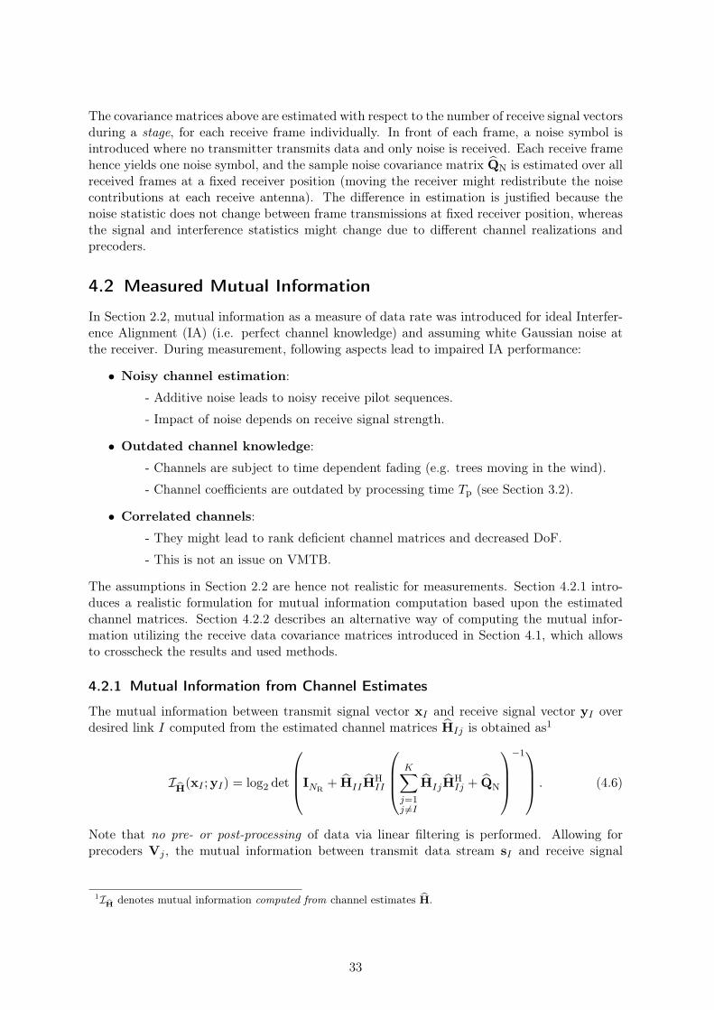
The covariance matrices above are estimated with respect to the number of receive signal vectorsduring a stage, for each receive frame individually. In front of each frame, a noise symbol isintroduced where no transmitter transmits data and only noise is received. Each receive framehence yields one noise symbol, and the sample noise covariance matrix QN is estimated over allreceived frames at a fixed receiver position (moving the receiver might redistribute the noisecontributions at each receive antenna). The difference in estimation is justified because thenoise statistic does not change between frame transmissions at fixed receiver position, whereasthe signal and interference statistics might change due to different channel realizations andprecoders.

4.2 Measured Mutual Information

In Section 2.2, mutual information as a measure of data rate was introduced for ideal Interfer-ence Alignment (IA) (i.e. perfect channel knowledge) and assuming white Gaussian noise atthe receiver. During measurement, following aspects lead to impaired IA performance:

• Noisy channel estimation:

- Additive noise leads to noisy receive pilot sequences.

- Impact of noise depends on receive signal strength.

• Outdated channel knowledge:

- Channels are subject to time dependent fading (e.g. trees moving in the wind).

- Channel coefficients are outdated by processing time Tp (see Section 3.2).

• Correlated channels:

- They might lead to rank deficient channel matrices and decreased DoF.

- This is not an issue on VMTB.

The assumptions in Section 2.2 are hence not realistic for measurements. Section 4.2.1 intro-duces a realistic formulation for mutual information computation based upon the estimatedchannel matrices. Section 4.2.2 describes an alternative way of computing the mutual infor-mation utilizing the receive data covariance matrices introduced in Section 4.1, which allowsto crosscheck the results and used methods.

4.2.1 Mutual Information from Channel Estimates

The mutual information between transmit signal vector xI and receive signal vector yI overdesired link I computed from the estimated channel matrices HIj is obtained as1

IH(xI ;yI) = log2 det

INR

+ HIIHHII

K∑

j=1j 6=I

HIjHHIj + QN

−1 . (4.6)

Note that no pre- or post-processing of data via linear filtering is performed. Allowing forprecoders Vj , the mutual information between transmit data stream sI and receive signal

1IH

denotes mutual information computed from channel estimates H.

33

vector yI is obtained as

IH(sI ;yI) = log2 det

INR

+ HIIVI

(HIIVI

)H

K∑

j=1j 6=I

HIjVj

(HIjVj

)H+ QN

−1 . (4.7)

If IA precoders are used, interference is aligned at the receiver. Finally including the receivefilters Ui as well, the mutual information between transmit data stream sI and receive datastream rI is obtained as

IH(sI ; rI) =

log2 det

Id +UH

I HIIVI

(UH

I HIIVI

)H

K∑

j=1j 6=I

UHI HIjVj

(UH

I HIjVj

)H+UH

I QNUI

−1 .

(4.8)If IA receive filters (i.e. interference suppression matrices) are used, the previously alignedinterference is suppressed.

In order to compare IA to other schemes, the precoding matrices and receive filters can bechosen accordingly. A natural approach is to perform a Singular Value Decomposition (SVD)(introduced in Equation (2.7)) on the channel estimates

HIj = LIΣIjRHj (4.9)

and use the right singular vectors as precoders Vj,SVD = Rj and the left singular vectors asreceive filters UI,SVD = LI . The transmit signal is thereby aligned along the NΣ (number ofsingular values) independent directions of the channel, decomposing the vector channel intoNΣ independent scalar channels:

UHI,SVDHIjVj,SVD = LH

I LIΣIjRHj Rj = ΣIj . (4.10)

Additionally, power allocation could be performed at the transmitters, considering the strengthof each “channel direction” (not done in this work). The mutual information computed fromchannel estimates using SVD filters is denoted I

H,SVD.

The mutual information over link I in the interference free case (single link) can be calculatedby setting the sums in Equation (4.6), Equation (4.7) and Equation (4.8) to zero. The mutualinformation computed from channel estimates in the absence of interference is denoted I

H,noInt.

The method of mutual information computation from channel estimation matrices is similarto emulation of IA with measured channels (transmission of pilot sequence would suffice). Themethod of truly transmitting data and compute the mutual information from the measuredreceive data covariance matrices is now discussed.

34

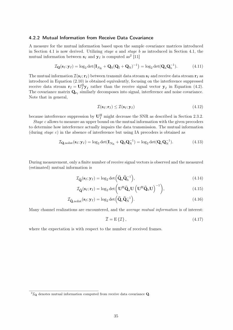
4.2.2 Mutual Information from Receive Data Covariance

A measure for the mutual information based upon the sample covariance matrices introducedin Section 4.1 is now derived. Utilizing stage a and stage b as introduced in Section 4.1, themutual information between sI and yI is computed as2 [11]

IQ(sI ;yI) = log2 det(INR

+QS(QI +QN)−1)= log2 det(QaQ

−1b ). (4.11)

The mutual information I(sI ; rI) between transmit data stream sI and receive data stream rI asintroduced in Equation (2.10) is obtained equivalently, focusing on the interference suppressedreceive data stream rI = UH

I yI rather than the receive signal vector yI in Equation (4.2).The covariance matrix QrI similarly decomposes into signal, interference and noise covariance.Note that in general,

I(sI ; rI) ≤ I(sI ;yI) (4.12)

because interference suppression by UHI might decrease the SNR as described in Section 2.3.2.

Stage c allows to measure an upper bound on the mutual information with the given precodersto determine how interference actually impairs the data transmission. The mutual information(during stage c) in the absence of interference but using IA precoders is obtained as

IQ,noInt(sI ;yI) = log2 det(INR+QSQ

−1N ) = log2 det(QcQ

−1N ). (4.13)

During measurement, only a finite number of receive signal vectors is observed and the measured(estimated) mutual information is

IQ(sI ;yI) = log2 det

(QaQ

−1b

), (4.14)

IQ(sI ; rI) = log2 det

(UHQaU

(UHQbU

)−1), (4.15)

IQ,noInt

(sI ;yI) = log2 det(QcQ

−1N

). (4.16)

Many channel realizations are encountered, and the average mutual information is of interest:

I = E {I} , (4.17)

where the expectation is with respect to the number of received frames.

2IQ denotes mutual information computed from receive data covariance Q.

35

4.3 Interference Suppression

Observing stage b as illustrated in Figure 4.1 over many frames, the estimated covariancematrices Qb yield information about the average alignment effort achieved by the precodingmatrices. The aim of IA is to restrict the interference in a NR − d dimensional subspace atthe receiver, which translates into rank(Qb) = NR − d in the absence of noise, because onlyinterference is received during stage b. A measure for this is now derived.

The concatenation of the interference suppression matrix UI and its orthogonal complementU⊥

I ∈ CNR×NR−d yields a unitary matrix

M =[UI U⊥

I

]. (4.18)

Remember that the received interference lies in the nullspace of UHI (Equation (2.18)) and

therefore in the column space of its orthogonal complement:

span(HIjVj

)⊆ span

((U⊥

I )H), ∀I 6= j. (4.19)

Utilizing MMH = INRand Condition (2.13a) in Equation (4.4) gives

Qb = MMHK∑

j=1j 6=I

HIjVjVHj H

HIj

︸ ︷︷ ︸QI

MMH +MMHQN

= M

MH

K∑

j=1j 6=I

HIjVjVHj H

HIj

M+QN

MH

= M

K∑

j=1j 6=I

UHI HIjVj︸ ︷︷ ︸

=0

VHj H

HIjUI UH

I HIjVj︸ ︷︷ ︸=0

VHj H

HIjU

⊥I

(U⊥

I

)HHIjVj V

Hj H

HIjUI︸ ︷︷ ︸

=0

(U⊥

I

)HHIjVjV

Hj H

HIjU

⊥I

+QN

MH

= M

([0 0

0(U⊥

I

)HQIU

⊥I

]+QN

)MH.

(4.20)

An eigenvalue decomposition is performed on the interference covariance term

(U⊥

I

)HQIU

⊥I = EΛEH, (4.21)

where E ∈ CNR−d×NR−d is unitary and Λ = diag{λ1, ..., λNR−d} contains the NR − d eigenval-

ues that correspond to the interference subspace in non-decreasing order. Incorporating theseresults in an eigenvalue decomposition of Qb in Equation (4.20) finally yields

Qb = M

[Id 0

0 E

]

︸ ︷︷ ︸E

([0 0

0 Λ

]+ΛN

)

︸ ︷︷ ︸Λ

[Id 0

0 E

]HMH

︸ ︷︷ ︸EH

, (4.22)

36

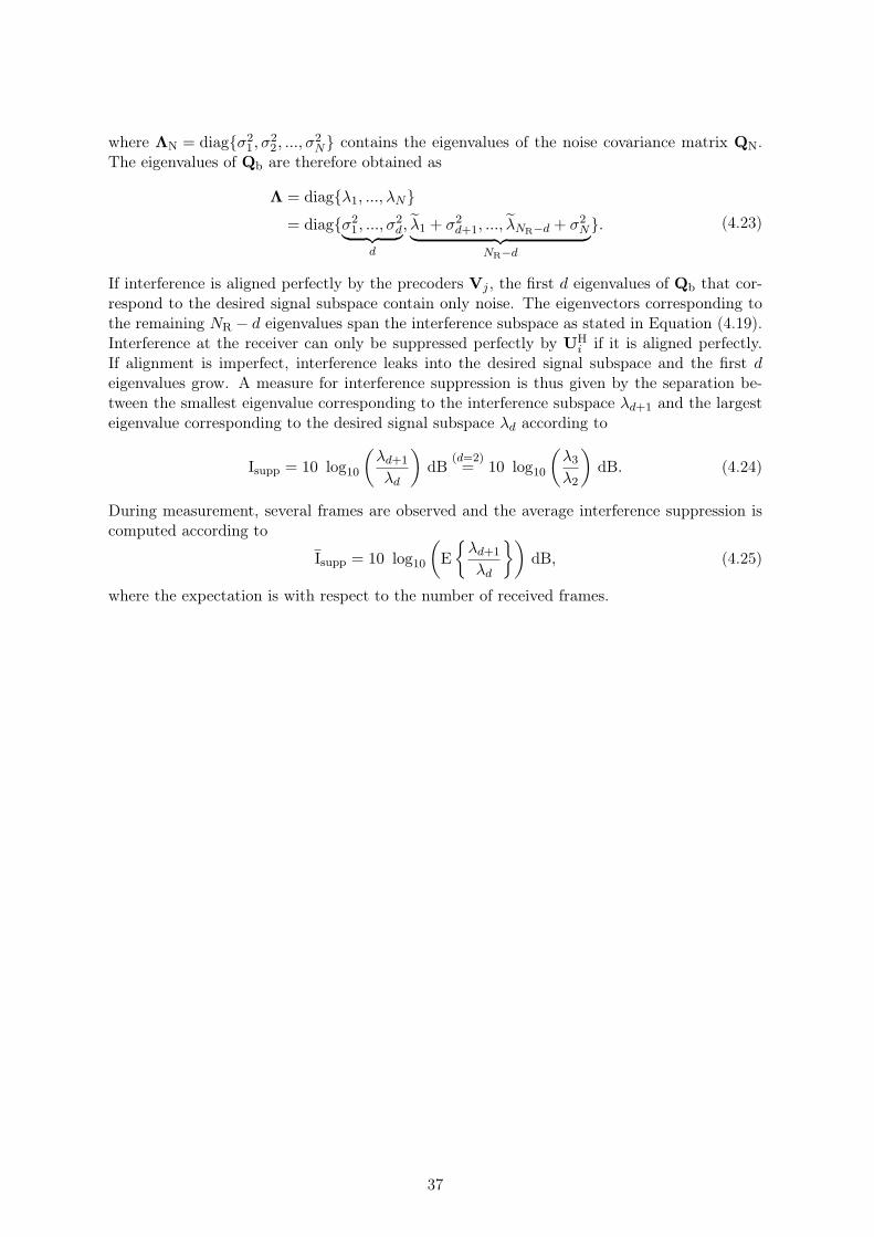
where ΛN = diag{σ21, σ

22, ..., σ

2N} contains the eigenvalues of the noise covariance matrix QN.

The eigenvalues of Qb are therefore obtained as

Λ = diag{λ1, ..., λN}= diag{σ2

1, ..., σ2d︸ ︷︷ ︸

d

, λ1 + σ2d+1, ..., λNR−d + σ2

N︸ ︷︷ ︸NR−d

}. (4.23)

If interference is aligned perfectly by the precoders Vj , the first d eigenvalues of Qb that cor-respond to the desired signal subspace contain only noise. The eigenvectors corresponding tothe remaining NR − d eigenvalues span the interference subspace as stated in Equation (4.19).Interference at the receiver can only be suppressed perfectly by UH

i if it is aligned perfectly.If alignment is imperfect, interference leaks into the desired signal subspace and the first deigenvalues grow. A measure for interference suppression is thus given by the separation be-tween the smallest eigenvalue corresponding to the interference subspace λd+1 and the largesteigenvalue corresponding to the desired signal subspace λd according to

Isupp = 10 log10

(λd+1

λd

)dB

(d=2)= 10 log10

(λ3

λ2

)dB. (4.24)

During measurement, several frames are observed and the average interference suppression iscomputed according to

Isupp = 10 log10

(E

{λd+1

λd

})dB, (4.25)

where the expectation is with respect to the number of received frames.

37

4.4 Power, SNR and SIR

The respective powers of signal, interference and noise are now defined in two ways, one isbased upon the sample covariance matrices introduced in Section 4.1, the other one utilizes theestimated channel matrices. Then, SNR and SIR which are computed from these powers aredefined.

The power of the desired signal at the receiver is obtained as

PQ,S

= trace(QS) = trace(Qc − QN). (4.26)

In theory, the power of the desired signal can also be computed as PQ,S

= trace(Qa − Qb).However, this leads to bad estimations in practice, especially if the interfering signals are a lotstronger than the desired signal. The desired signal “vanishes” in the much stronger interference.The power of the interference at the receiver is obtained as

PQ,I

= trace(QI) = trace(Qb − QN), (4.27)

the power of the noise at the receiver is

PQ,N

= trace(QN). (4.28)

An alternative method of power computation considers the estimated channel matrices HIj .The receive power contribution from transmitter j to receiver I is computed as

PIj = trace(HIjH

HIj

)=∥∥∥HIj

∥∥∥2

F. (4.29)

Note that this formulation considers the pure channel without filters Vj , UI . Also note thatcontrolled transmit power variations realized via the programmable RF attenuators are in-cluded in the estimated channel matrices (RF attenuators are part of the channel). A measurethat compares to the powers defined in Equation (4.26) and Equation (4.27) needs to includethe precoders (transmit filters), since they are implicitly contained in the sample covariancematrices. Furthermore, the impact of the interference suppression matrices (receive filters) canalso be investigated by including them in the formulation. The receive power contribution ofthe desired transmitter, for each of the three cases, is defined as

PH,S

=∥∥∥HII

∥∥∥2

F, (4.30a)

PHV,S

=∥∥∥HIIVI

∥∥∥2

F, (4.30b)

PUHV,S

=∥∥∥UH

I HIIVI

∥∥∥2

F. (4.30c)

Similarly, the receive power contribution of the interfering transmitters (interference power),for each of the three cases, is defined as

PH,I

=K∑

j=1j 6=I

∥∥∥HIj

∥∥∥2

F, (4.31a)

PHV,I

=

K∑

j=1j 6=I

∥∥∥HIjVj

∥∥∥2

F, (4.31b)

PUHV,I

=K∑

j=1j 6=I

∥∥∥UIHIjVj

∥∥∥2

F. (4.31c)

38

Many frames are observed and the mean power is of interest:

P = E {P} , (4.32)

where the expectation is with respect to the number of received frames. Note that the samplecovariance matrices and the channel estimation matrices are estimated on frame basis (i.e. eachframe yields a matrix). The only exception is the noise covariance matrix, which is estimatedover all frames at a fixed receiver position, because each frame contains only one noise symbol.The SNR is now computed as

SNRQ= 10 log10

(P

Q,S

PQ,N

)dB, (4.33)

the SIR as

SIRQ= 10 log10

(P

Q,S

PQ,I

)dB. (4.34)

An alternative SNR computation utilizing the channel estimation matrices is given by

SNRH

= 10 log10

(P

H,S

PQ,N

)dB, (4.35a)

SNRHV

= 10 log10

(P

HV,S

PQ,N

)dB, (4.35b)

SNRUHV

= 10 log10

(P

UHV,S

PQ,N

)dB. (4.35c)

Similarly, SIR is computed from the channel estimation matrices according to

SIRH

= 10 log10

(P

H,S

PH,I

)dB, (4.36a)

SIRHV

= 10 log10

(P

HV,S

PHV,I

)dB, (4.36b)

SIRUHV

= 10 log10

(P

UHV,S

PUHV,I

)dB. (4.36c)

SNRQ

compares to SNRHV

and SIRQ

compares to SIRHV

, which will be proven by measure-ments in Section 5.2.1 and Section 5.3.1.

For the following, keep in mind that SNR and SIR are implicitly averaged over all trans-missions, which usually include many receiver positions to average over small scale fading. Acertain SNR or SIR value is achieved on average over all transmissions.

39

Chapter 5

Measurements

Section 5.1 shows the feasibility of IA at fixed SNR and SIR and explains how the subsequentmeasurements are performed. Section 5.2 investigates how the performance measures intro-duced in Chapter 4 depend on variable SNR at fixed SIR. Section 5.3 does the same for variableSIR, keeping the SNR fixed.

5.1 Validation of Interference Alignment

The feasibility of IA on the Vienna MIMO Testbed (VMTB) is now shown utilizing the perfor-mance measures introduced in Chapter 4. This section establishes the basic methodology forthe subsequent measurements in Section 5.2 and Section 5.3. All three links are desired onceto compare the results. Figure 5.1 subsumes the measurement process.

attenuator constellations

receiver positions

frame transmissions

1

1 1 1 1 11 1 1 1 11 1 1 1 1

1 1 1 1

1 2 3 5

2 2 2 2 23 3 3 3 3desired links

50

4

Figure 5.1: Validation: measurement process

Note following aspects of the illustration:

• receiver positions: 5 receiver positions (RX antennas positioned in x-y-φ) were realized.

• desired links: At each position, transmitters I = {1, 2, 3} were desired once.

• attenuator constellations: For each desired link, one RF transmit-attenuator constel-lation was utilized to achieve SIR = −3 dB.

• frame transmissions: 50 frames were transmitted at one attenuator constellation ofone receiver position.

The layer-order coincides with the actual measurement process - receiver repositioning is the“outer loop” of the measurement. Table 5.1 depicts the parameters of the validation measure-ment.

Figure 5.2, Figure 5.3 and Figure 5.4 (one figure for each desired link) show the eigenvaluesof Qb and QN, denoted {λ1, ..., λ4} and {σ2

1, ..., σ24}, respectively. Remember that each point

corresponds to one frame evaluation, and that Qb is estimated during stage b where only theinterferers transmit. The eigenvalues are plotted logarithmically and normalized so that λ2 liesat 0 dB on average. Ideally, λ1 and λ2 that correspond to the desired signal subspace would

40

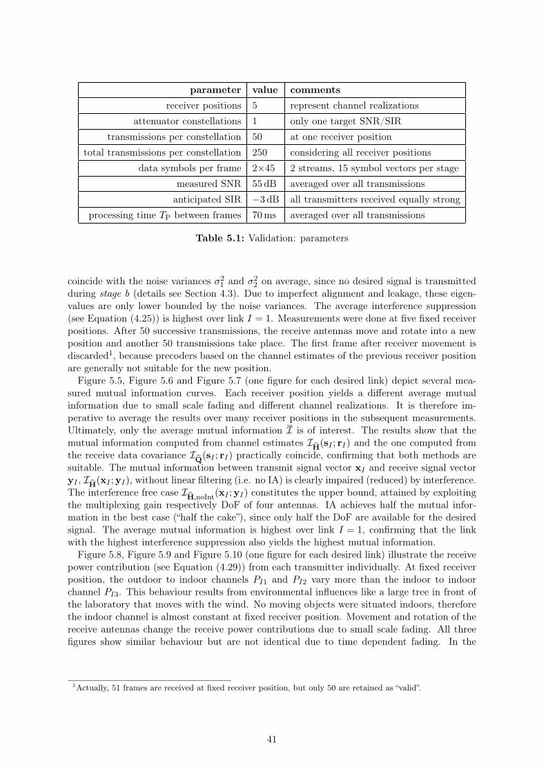
parameter value comments

receiver positions 5 represent channel realizations

attenuator constellations 1 only one target SNR/SIR

transmissions per constellation 50 at one receiver position

total transmissions per constellation 250 considering all receiver positions

data symbols per frame 2×45 2 streams, 15 symbol vectors per stage

measured SNR 55 dB averaged over all transmissions

anticipated SIR −3 dB all transmitters received equally strong

processing time TP between frames 70ms averaged over all transmissions

Table 5.1: Validation: parameters

coincide with the noise variances σ21 and σ2

2 on average, since no desired signal is transmittedduring stage b (details see Section 4.3). Due to imperfect alignment and leakage, these eigen-values are only lower bounded by the noise variances. The average interference suppression(see Equation (4.25)) is highest over link I = 1. Measurements were done at five fixed receiverpositions. After 50 successive transmissions, the receive antennas move and rotate into a newposition and another 50 transmissions take place. The first frame after receiver movement isdiscarded1, because precoders based on the channel estimates of the previous receiver positionare generally not suitable for the new position.

Figure 5.5, Figure 5.6 and Figure 5.7 (one figure for each desired link) depict several mea-sured mutual information curves. Each receiver position yields a different average mutualinformation due to small scale fading and different channel realizations. It is therefore im-perative to average the results over many receiver positions in the subsequent measurements.Ultimately, only the average mutual information I is of interest. The results show that themutual information computed from channel estimates I

H(sI ; rI) and the one computed from

the receive data covariance IQ(sI ; rI) practically coincide, confirming that both methods are

suitable. The mutual information between transmit signal vector xI and receive signal vectoryI , IH(xI ;yI), without linear filtering (i.e. no IA) is clearly impaired (reduced) by interference.The interference free case I

H,noInt(xI ;yI) constitutes the upper bound, attained by exploiting

the multiplexing gain respectively DoF of four antennas. IA achieves half the mutual infor-mation in the best case (“half the cake”), since only half the DoF are available for the desiredsignal. The average mutual information is highest over link I = 1, confirming that the linkwith the highest interference suppression also yields the highest mutual information.

Figure 5.8, Figure 5.9 and Figure 5.10 (one figure for each desired link) illustrate the receivepower contribution (see Equation (4.29)) from each transmitter individually. At fixed receiverposition, the outdoor to indoor channels PI1 and PI2 vary more than the indoor to indoorchannel PI3. This behaviour results from environmental influences like a large tree in front ofthe laboratory that moves with the wind. No moving objects were situated indoors, thereforethe indoor channel is almost constant at fixed receiver position. Movement and rotation of thereceive antennas change the receive power contributions due to small scale fading. All threefigures show similar behaviour but are not identical due to time dependent fading. In the

1Actually, 51 frames are received at fixed receiver position, but only 50 are retained as “valid”.

41

subsequent measurements, the average (over all frames) receive power contributions are calcu-lated and the programmable RF transmit-attenuators are chosen to control the SNR and SIRaccordingly. In this measurement, the three transmitters were received about equally strong onaverage, hence SIR ≈ −3 dB as the interference is twice as strong as the desired signal. Overall,the channels are very static at fixed receiver position.

The results show that IA works and interference is aligned at the receiver. The better thealignment, the higher the interference suppression (separation between λ2 and λ3) and thehigher the mutual information. Channels are quasi-static at fixed receiver position. For thesubsequent measurements where SNR and SIR are varied, the results are averaged over allframes of a specific attenuator constellation, which includes several receiver positions to averageover small scale fading. Attenuator constellation refers to a specific choice of the RF transmit-attenuators, in the following just called attenuators, chosen to achieve a certain SNR or SIRvalue.

Isupp = 49.2 dB

Figure 5.2: Validation: eigenvalues of Qb and QN (desired link I = 1)

42

Isupp = 42.3 dB

Figure 5.3: Validation: eigenvalues of Qb and QN (desired link I = 2)

Isupp = 46.3 dB

Figure 5.4: Validation: eigenvalues of Qb and QN (desired link I = 3)

43

0 50 100 150 200 2500

10

20

30

40

50

60

70

80

frame transmissions

mutu

al info

rmat

ion [bit/s

/Hz]

IbQ(s1; r1)

I bH(s1; r1)

I bH(s1; r1)

I bH(x1;y1)

I bH,noInt(x1;y1)

Figure 5.5: Validation: mutual information comparison (desired link I = 1)

0 50 100 150 200 2500

10

20

30

40

50

60

70

frame transmissions

mutu

al info

rmat

ion [bit/s

/Hz]

IbQ(s1; r1)

I bH(s1; r1)

I bH(s1; r1)

I bH(x1;y1)

I bH,noInt(x1;y1)

Figure 5.6: Validation: mutual information comparison (desired link I = 2)

44

0 50 100 150 200 2500

10

20

30

40

50

60

70

80

frame transmissions

mutu

al info

rmat

ion [bit/s

/Hz]

IbQ(s1; r1)

I bH(s1; r1)

I bH(s1; r1)

I bH(x1;y1)

I bH,noInt(x1;y1)

Figure 5.7: Validation: mutual information comparison (desired link I = 3)

0 50 100 150 200 25047

47.5

48

48.5

49

49.5

50

50.5

51

51.5

frame transmissions

(indoor)

P11

P12

P13

10lo

g10(P

1j)

[dB

]

Figure 5.8: Validation: receive power contributions (desired link I = 1)

45

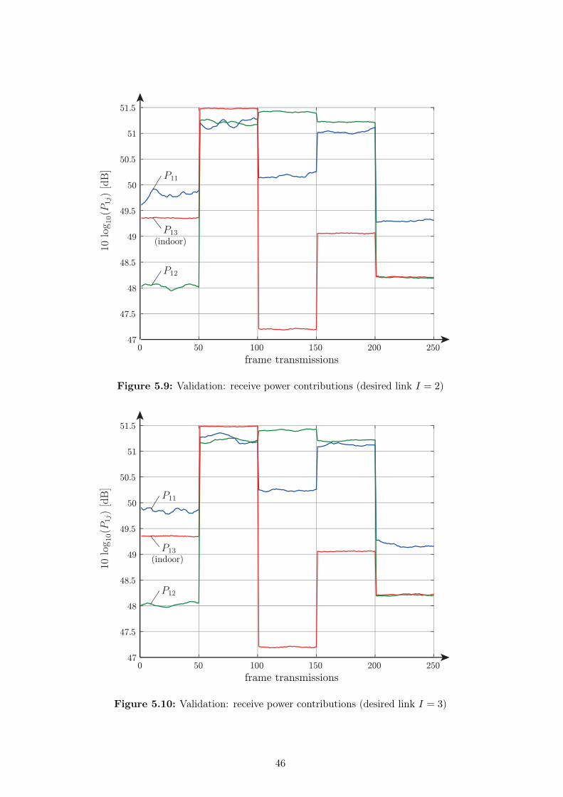
0 50 100 150 200 25047

47.5

48

48.5

49

49.5

50

50.5

51

51.5

frame transmissions

10lo

g10(P

1j)

[dB

]

P11

P12

P13

(indoor)

Figure 5.9: Validation: receive power contributions (desired link I = 2)

0 50 100 150 200 25047

47.5

48

48.5

49

49.5

50

50.5

51

51.5

frame transmissions

10lo

g10(P

1j)

[dB

]

P11

P12

P13

(indoor)

Figure 5.10: Validation: receive power contributions (desired link I = 3)

46

5.2 Variable SNR at Fixed SIR

The dependence of mutual information and other measures on SNR at fixed SIR = −3 dB isnow investigated. The necessary transmit power calibration can be summarized as follows:

1. Measure the average receive power contributions P Ij according to Equation (4.29) overall receiver positions at lowest possible attenuator values αj,init = 0 dB.

2. Consider the lowest average channel power:

Pmin = minj

P Ij , j = {1, 2, 3}.

3. Compute the attenuator increments according to:

∆αj =⌊10 log10

(P Ij

Pmin

)⌋dB.

4. Compute the final attenuator values according to:

αj = αj,init +∆αj .

5. Reduce SNR by increasing all attenuator values simultaneously by a certain stepsize.

This results in constant average SIR = −3 dB, since all three transmitters are received equallystrong (within +/− 1 dB) on average. Figure 5.11 illustrates the measurement process.

attenuator constellations

receiver positions

frame transmissions

1

1 1

30

1 12 23 318 1819 1920 20

desired links

50

1 20

Figure 5.11: Variable SNR: measurement process

The parameters of the the measurement are summarized in Table 5.2.

parameter value comments

receiver positions 30 represent channel realizations

attenuator constellations 20 relative attenuator values: 0, 3, ..., 57 dB

transmissions per constellation 50 at one receiver position

total transmissions per constellation 1500 considering all receiver positions

data symbols per frame 2×60 2 streams, 20 symbol vectors per stage

anticipated SNR 16...73 dB

anticipated SIR −3 dB all transmitters received equally strong

processing time TP between frames 70ms averaged over all transmissions

Table 5.2: Variable SNR: parameters

47

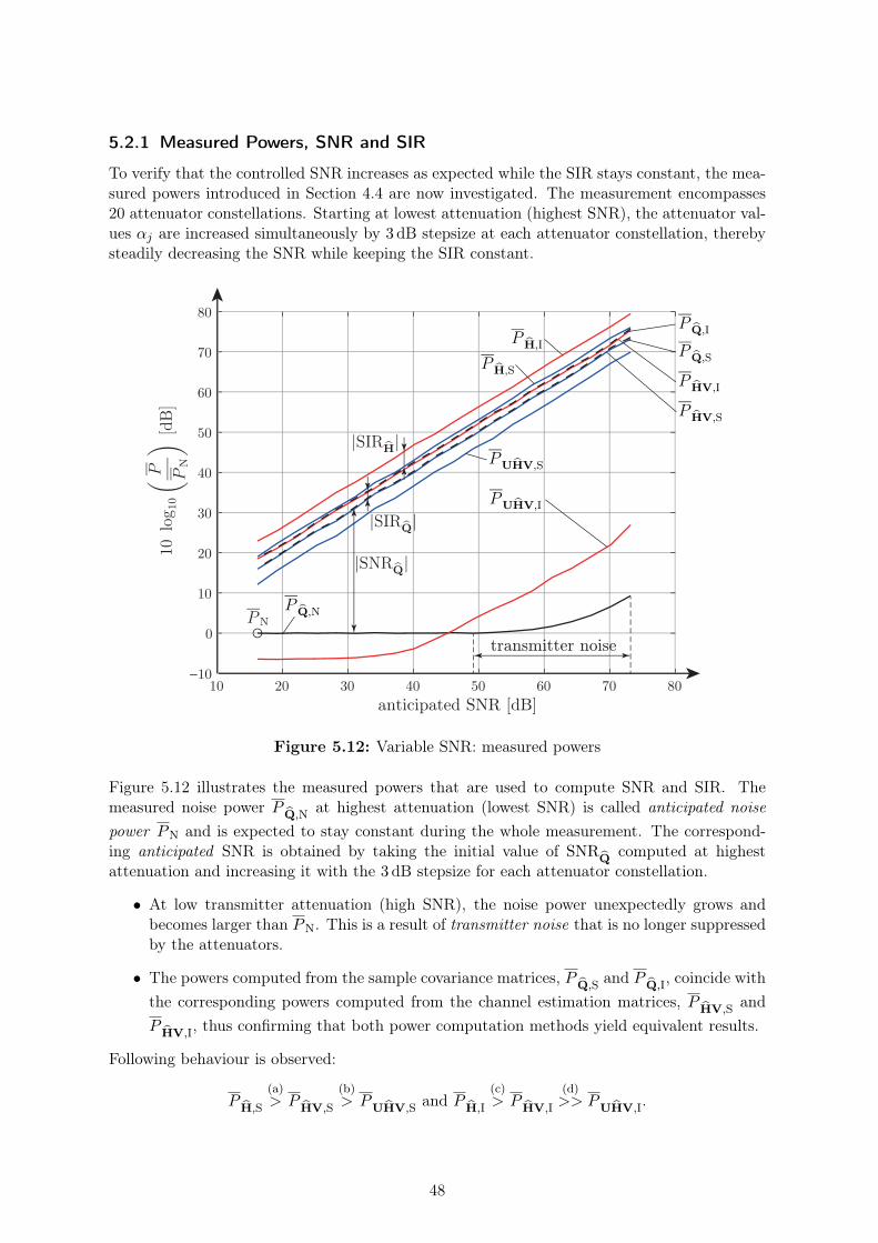
5.2.1 Measured Powers, SNR and SIR

To verify that the controlled SNR increases as expected while the SIR stays constant, the mea-sured powers introduced in Section 4.4 are now investigated. The measurement encompasses20 attenuator constellations. Starting at lowest attenuation (highest SNR), the attenuator val-ues αj are increased simultaneously by 3 dB stepsize at each attenuator constellation, therebysteadily decreasing the SNR while keeping the SIR constant.

|SNRbQ|

|SIRbQ|

|SIR bH|

Figure 5.12: Variable SNR: measured powers

Figure 5.12 illustrates the measured powers that are used to compute SNR and SIR. Themeasured noise power P

Q,Nat highest attenuation (lowest SNR) is called anticipated noise

power PN and is expected to stay constant during the whole measurement. The correspond-ing anticipated SNR is obtained by taking the initial value of SNR

Qcomputed at highest

attenuation and increasing it with the 3 dB stepsize for each attenuator constellation.

• At low transmitter attenuation (high SNR), the noise power unexpectedly grows andbecomes larger than PN. This is a result of transmitter noise that is no longer suppressedby the attenuators.

• The powers computed from the sample covariance matrices, PQ,S

and PQ,I

, coincide with

the corresponding powers computed from the channel estimation matrices, PHV,S

and

PHV,I

, thus confirming that both power computation methods yield equivalent results.

Following behaviour is observed:

PH,S

(a)> P

HV,S

(b)> P

UHV,Sand P

H,I

(c)> P

HV,I

(d)>> P

UHV,I.

48

This can be explained as follows:

(a) Precoding (see Equation 2.1) performs a basis transformation on the transmit data streamand arranges the d = 2 signal dimensions in a MT = 4 dimensional space. The precodingmatrix Vj is a truncated unitary matrix of dimension MT × d. The product HIIVI hasthe property

PHV,S

=∥∥∥HIIVI

∥∥∥2

F<∥∥∥HII

∥∥∥2

F= P

H,S, (5.1)

assuming HII has full rank.Proof (indices are dropped): The truncated unitary matrix V can be written as theproduct of a true unitary matrix V′ and a truncated identity matrix according to

V = V′

[Id

0

].

Furthermore,

HV′ =[Hd HMT−d

]and

∥∥∥H∥∥∥2

F=∥∥∥HV′

∥∥∥2

F.

Considering this in the left hand side of Equation (5.1):

PHV,S

=∥∥∥HV

∥∥∥2

F=

∥∥∥∥∥HV′

[Id

0

]∥∥∥∥∥

2

F

=

∥∥∥∥∥[Hd HMT−d

] [ Id

0

]∥∥∥∥∥

2

F

=∥∥∥Hd

∥∥∥2

F.

The right hand side of Equation (5.1) is treated similarly:

PH,S

=∥∥∥H∥∥∥2

F=∥∥∥HV′

∥∥∥2

F=∥∥∥[Hd HMT−d

]∥∥∥2

F

= trace

([Hd HMT−d

] [ HHd

HHMT−d

])

= trace(HdH

Hd

)+ trace

(HMT−dH

HMT−d

)

=∥∥∥Hd

∥∥∥2

F+∥∥∥HMT−d

∥∥∥2

F.

Comparing both sides:

PHV,S

=∥∥∥Hd

∥∥∥2

F<∥∥∥Hd

∥∥∥2

F+∥∥∥HMT−d

∥∥∥2

F= P

H,S.

This proves that precoding reduces the power.

(b) Interference suppression lowers the power of the desired signal. As mentioned in Sec-tion 2.3.2, the closed form computation of the IA filters has no constraint on maximizingthe SNR. A reasoning similar to (a) applies (UI is a truncated unitary matrix).

(c) Each interferer uses precoding matrices, interference power is hence also reduced by pre-coding. The same reasoning as in (a) applies.

(d) Interference suppression tries to suppress the interference power completely (rememberEquation 2.18). Ideally, P

UHV,Iwould be zero at all times. Above 40 dB SNR, P

UHV,I

starts to grow and is constantly 50 dB lower than PH,I

- the (non-ideal) IA filters are ableto lower the interference power by approximately 50 dB. The effect of growing interferencepower will be further studied in Section 5.2.2.

49

Note that SIRH

is used as reference to control the SIR (via attenuators), since it considers the“true” power contribution from each transmitter without transmit or receive filters.

Figure 5.13 shows the measured SNR and SIR curves.

• SNRQ

follows the anticipated SNR line nicely until it is lowered by the received trans-mitter noise, noticeable above 60 dB SNR.

• SNRH

> SNRQ(≈ SNR

HV) > SNR

UHV, evident from explanations (a) and (b) above.

• SIRH

follows the anticipated SIR line (−3 dB) nicely since it was used as reference fortransmit power calibration.

• SIRUHV

is the actual SIR after interference suppression and shows impressive results.

10 20 30 40 50 60 70 80−10

0

10

20

30

40

50

60

70

80

anticipated SNR [dB]

measured SNR and SIR

 [dB]

anticipated SNR

anticipated SIR

SNRbQ

SNR bH

SNRU bHV

SIRU bHV

SIR bH

SIRbQ

Figure 5.13: Variable SNR: measured SNR and SIR

50

5.2.2 Interference Suppression

Figure 5.14 depicts the average interference suppression as defined in Equation (4.25). Themeasured SNR

Qis also plotted for comparison. In Figure 5.12, it was confirmed that signal

and interference power steadily increase with increasing SNR. Increasing interference powercorresponds to growing eigenvalues λ3 and λ4 of Qb, and the associated Isupp would ideallyalso increase in the same manner. However, it peaks out at around 60 dB SNR and theneven decreases. Intuitively, this could be caused by received transmitter noise or by leakageof the interference (λ3 and λ4) into the desired signal subspace (λ1 and λ2) as a result of badalignment.

10 20 30 40 50 60 70 8015

20

25

30

35

40

45

50

55

60

65

anticipated SNR [dB]

average interference suppression [dB]

Isupp

SNRbQ

Figure 5.14: Variable SNR: average interference suppression

Figure 5.15 shows the eigenvalues of Qb (denoted {λ1, ..., λ4}) and QN (denoted{σ21, ..., σ

24

}),

averaged over all transmissions and plotted for each attenuator constellation (SNR realization).It becomes apparent that the effect of growing noise (received transmitter noise) at high SNRis not the only cause of the reduced interference suppression, as it starts at around 60 dB SNRwhereas the leakage phenomenon starts already around 40 dB SNR. The increased leakage iscaused by outdated precoders that are computed from the channel estimates of “the last framerather than the actual frame” (see Section 3.2). This is a systematic error in the measurementmethodology that can not be circumvented. Due to the sequential nature of channel estimation→ filter computation → filter feedback, filters are always outdated by Tp = 70ms. An interfer-ence suppression of 50 dB is “as good as it gets” considering the used measurement methodologyand the experienced channel fluctuations. If ideal precoders (from perfect channel knowledge)would be used, leakage would not occur.

51

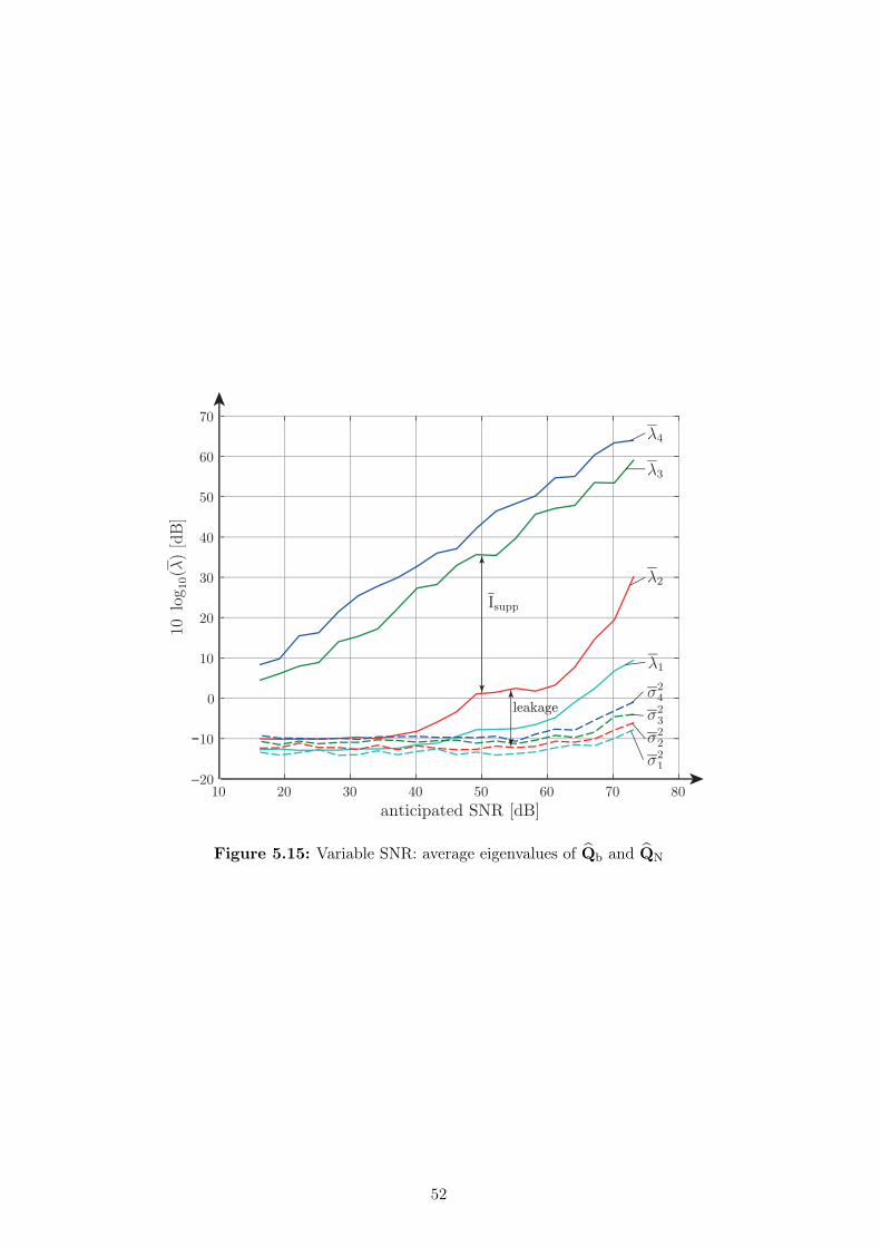
10 20 30 40 50 60 70 80−20

−10

0

10

20

30

40

50

60

70

anticipated SNR [dB]

10log10(λ)[dB]

σ21

σ22

σ23

σ24

Isupp

leakage

λ2

λ4

λ3

λ1

Figure 5.15: Variable SNR: average eigenvalues of Qb and QN

52

5.2.3 Mutual Information

Figure 5.16 illustrates various measured mutual information curves. The upper bound is con-stituted by I

H,noInt(x1;y1), which coincides with I

H,SVD,noInt(s1; r1) (not plotted here) and

is only achievable in the absence of interference by exploiting all four DoF provided by fourantenna MIMO transmission. The lowest mutual information is given by I

H(x1;y1), which

coincides with IH,SVD

(s1;y1) (not plotted here) and heavily suffers from interference. It isnot visibly affected by SNR variations, because the interference power is the dominant powerthroughout the whole measurement (PI >> PN). In between, IA tries to optimally exploit itstwo DoF and would ideally attain “half the cake”, meaning half of the the upper bound. Thisseems to be true only in the low SNR regime of the plot, as the gap between mutual informa-tion with and without interference present grows with increasing SNR. The worsened mutualinformation at high SNR is a result of the leakage phenomenon discovered in Section 5.2.2.

10 20 30 40 50 60 70 800

10

20

30

40

50

60

70

80

90

anticipated SNR [dB]

mutu

al info

rmat

ion [bit/s

/Hz]

"half the cake"

IA filters

uppe

r bou

nd, n

o interfe

renc

e

I bH,noInt(x1;y1)

I bH(x1;y1)

I bH(s1; r1)

I bQ(s1; r1)

I bQ,noInt(s1; r1)

I bH,noInt(s1; r1)

Figure 5.16: Variable SNR: mutual information (overview)

Figure 5.17 focuses on mutual information in the presence of interference. The lower curvesshow the mutual information with SVD filters as defined in Section 4.2.1. Note that these filtersutilize all four DoF but are computed as if no interference is present (each user assumes a singlelink). Using IA filters (i.e. IA precoding and interference suppression matrices), the resultsare improved considerably. Apparently, mutual information is lowered by receive filtering. ForIA, this behaviour was already mentioned in Section 2.3.2 and in Section 5.2.1. Imagine thatinterference is aligned in a subspace at the receiver. This subspace is linearly independentof the desired signal subspace, but not necessarily orthogonal to it. Interference suppressionthat projects the desired signal onto a subspace that is orthogonal to the interference subspacetherefore lowers the SNR. Another interpretation considers the mutual information. Thereceive signal vector yI contains a certain amount of information about the transmit signal

53

stream sI , but interference is still present. Part of this information is “cut away” in the processof interference suppression and is missing in the receive symbol stream rI .

10 20 30 40 50 60 70 800

5

10

15

20

25

30

35

anticipated SNR [dB]

mutual inform

ation [bit/s/H

z]

SNR reduction

SVD filters

IA filters

I bH(s1;y1)

I bQ(s1;y1)

I bQ(s1; r1)

I bH(s1; r1)

I bH,SVD(s1; r1)

I bH,SVD(s1;y1)

Figure 5.17: Variable SNR: mutual information

The measurements above demonstrated that in the low SNR regime of the plots, IA worksas expected in theory and achieves superb results. Note that the low SNR regime actuallyconsiders relatively high SNR values. The focus of the measurements was clearly set on highSNR values, provoking hardware-induced effects which diminish the IA performance. In orderto realize lower SNR values, the “DACscaling” (see Equation (3.4)) has to be lowered, whichin turn introduces heightened quantization noise. This exceeds the focus of this work.

54

5.3 Variable SIR at Fixed SNR

The dependence of the performance measures on SIR at fixed SNR = 37 dB is now investigated.The transmit power calibration is performed similarly to the method described in Section 5.2,only step 5 is altered in order to vary the SIR. With the final attenuator values as obtainedin step 4, all transmitters are received equally strong (SNR = −3 dB) and have maximumpower (lowest attenuation). The desired transmitter attenuator αI is then increased to obtaina certain (fixed) SNR value. Finally, the interfering transmitter attenuators αj , j 6= I, arejointly increased in order to increase the SIR. An example will illuminate the process:

1. Final attenuator values after transmit power calibration (see Section 5.2):

[α1, α2, α3] = [0, 2, 6] dBaccomplish→ SNR = 73 dB, SIR = −3 dB.

2. Increase desired transmitter attenuator α1 (desired link I = 1) by 36 dB in order to obtainSNR = 37 dB:

[α1 + 36, α2, α3] = [36, 2, 6] dB → SNR = 73− 36 = 37 dB, SIR = −3− 36 = −39 dB.

3. Assuming 3 dB increment of α2 and α3 (interfering transmitter attenuators) at eachattenuator constellation, this results in following anticipated SIR range:

attenuator constellation 1: [36, 2, 6] dB → SNR = 37 dB, SIR = −39 dB,attenuator constellation 2: [36, 5, 9] dB → SNR = 37 dB, SIR = −36 dB,attenuator constellation 3: [36, 8, 12] dB → SNR = 37 dB, SIR = −33 dB,

...attenuator constellation 20:[36, 59, 63] dB → SNR = 37 dB, SIR = 18 dB.

Figure 5.11 illustrates the measurement process. In this measurement, all three links weredesired once.

20 2020 2020 20attenuator constellations

receiver positions

frame transmissions

1

1 12 23 3

30

1 11 11 11

desired links

30

20

Figure 5.18: Variable SIR: measurement process

The parameters of the the measurement are summarized in Table 5.3.

5.3.1 Measured Powers, SNR and SIR

To verify that the controlled SIR increases as expected while the SNR stays constant, themeasured powers are now investigated. The measurement encompasses 20 attenuator constel-lations.

Figure 5.19 illustrates the measured powers that are used to compute SNR and SIR. Themeasured noise power P

Q,Nat highest interferer attenuation (highest SIR) is called anticipated

noise power PN and is expected to stay constant during the whole measurement. The cor-responding anticipated SNR is also expected to stay constant at 37 dB, SNR

Qconstitutes its

55

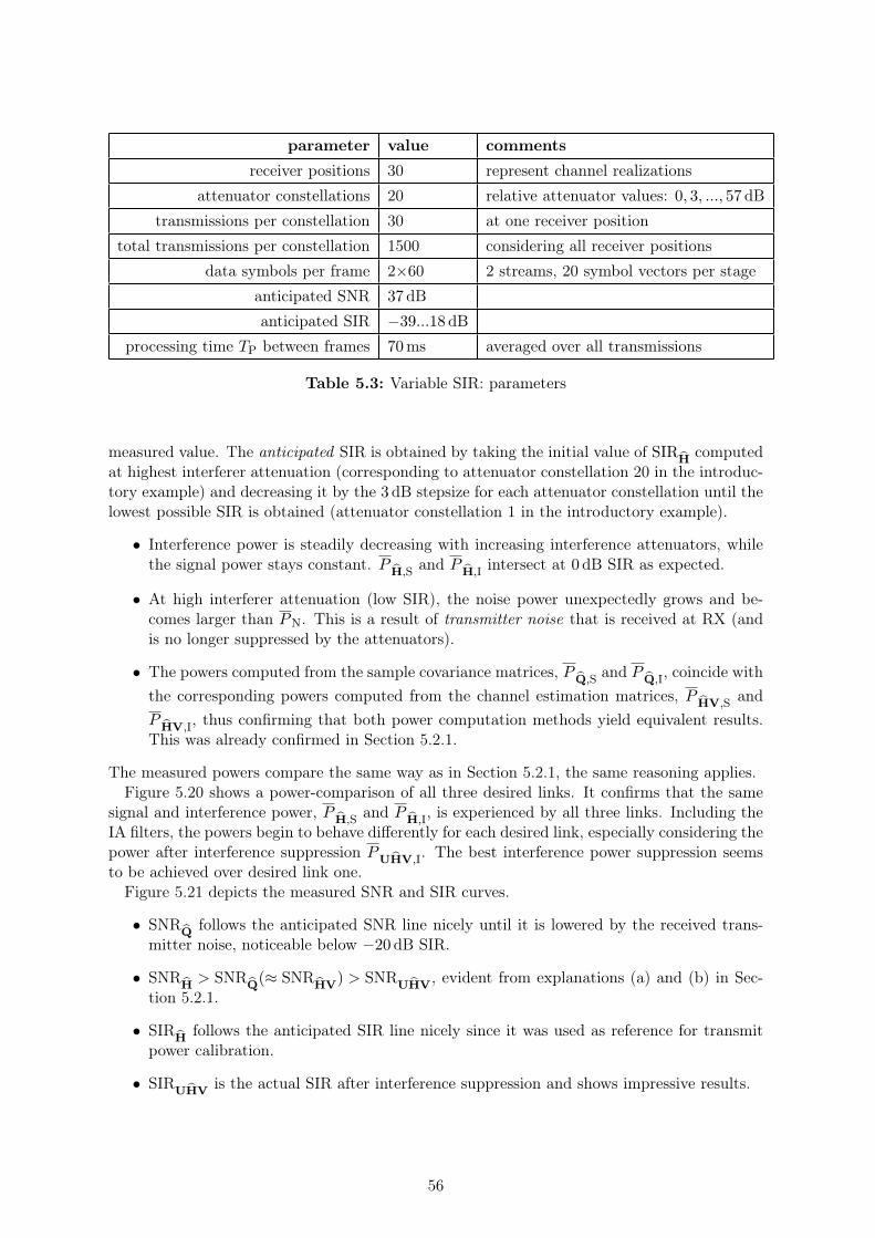
parameter value comments

receiver positions 30 represent channel realizations

attenuator constellations 20 relative attenuator values: 0, 3, ..., 57 dB

transmissions per constellation 30 at one receiver position

total transmissions per constellation 1500 considering all receiver positions

data symbols per frame 2×60 2 streams, 20 symbol vectors per stage

anticipated SNR 37 dB

anticipated SIR −39...18 dB

processing time TP between frames 70ms averaged over all transmissions

Table 5.3: Variable SIR: parameters

measured value. The anticipated SIR is obtained by taking the initial value of SIRH

computedat highest interferer attenuation (corresponding to attenuator constellation 20 in the introduc-tory example) and decreasing it by the 3 dB stepsize for each attenuator constellation until thelowest possible SIR is obtained (attenuator constellation 1 in the introductory example).

• Interference power is steadily decreasing with increasing interference attenuators, whilethe signal power stays constant. P

H,Sand P

H,Iintersect at 0 dB SIR as expected.

• At high interferer attenuation (low SIR), the noise power unexpectedly grows and be-comes larger than PN. This is a result of transmitter noise that is received at RX (andis no longer suppressed by the attenuators).

• The powers computed from the sample covariance matrices, PQ,S

and PQ,I

, coincide with

the corresponding powers computed from the channel estimation matrices, PHV,S

and

PHV,I

, thus confirming that both power computation methods yield equivalent results.This was already confirmed in Section 5.2.1.

The measured powers compare the same way as in Section 5.2.1, the same reasoning applies.Figure 5.20 shows a power-comparison of all three desired links. It confirms that the same

signal and interference power, PH,S

and PH,I

, is experienced by all three links. Including theIA filters, the powers begin to behave differently for each desired link, especially considering thepower after interference suppression P

UHV,I. The best interference power suppression seems

to be achieved over desired link one.Figure 5.21 depicts the measured SNR and SIR curves.

• SNRQ

follows the anticipated SNR line nicely until it is lowered by the received trans-mitter noise, noticeable below −20 dB SIR.

• SNRH

> SNRQ(≈ SNR

HV) > SNR

UHV, evident from explanations (a) and (b) in Sec-

tion 5.2.1.

• SIRH

follows the anticipated SIR line nicely since it was used as reference for transmitpower calibration.

• SIRUHV

is the actual SIR after interference suppression and shows impressive results.

56

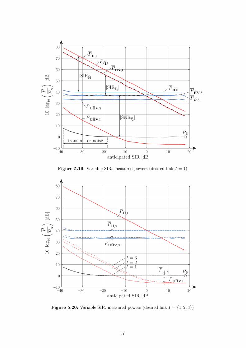
|SIR bH|

|SIRbQ|

|SNRbQ|

Figure 5.19: Variable SIR: measured powers (desired link I = 1)

−40 −30 −20 −10 0 10 20−10

0

10

20

30

40

50

60

70

80

anticipated SIR [dB]

PU bHV,S

PU bHV,I

P bH,S

P bH,I

PNP bQ,N

10log10

(P PN

)[dB]

I = 1

I = 3I = 2

Figure 5.20: Variable SIR: measured powers (desired link I = {1, 2, 3})

57

−40 −30 −20 −10 0 10 20−40

−30

−20

−10

0

10

20

30

40

50

anticipated SIR [dB]

measured SNR and SIR

 [dB] SNRbQ

SIR bH

SNR bH

SNRU bHV

SIRU bHV

SIRbQ

anticipated SNR

anticipated SIR

Figure 5.21: Variable SIR: measured SNR and SIR (desired link I = 1)

58

5.3.2 Interference Suppression

Figure 5.22 depicts the average interference suppression as defined in Equation (4.25), for eachlink individually. It behaves as expected at moderate and high SIR - growing interferencepower results in growing interference suppression. It peaks out at around −25 dB SIR andeven decreases for smaller SIR. Two effects have to be considered:

• The leakage phenomenon, discovered in Section 5.2.2, will also occur at low SIR (stronginterference). It is mainly caused by outdated precoders (see Section 3.2). Similar toSection 5.2.2, an interference suppression of 50 dB is “as good as it gets”.

• Below −20 dB SIR, received transmitter noise becomes noticeable.

−40 −30 −20 −10 0 10 2010

15

20

25

30

35

40

45

50

55

anticipated SIR [dB]

average interference suppression [dB]

Isupp

I = 3

I = 1

I = 2

Figure 5.22: Variable SIR: average interference suppression (desired link I = {1, 2, 3})

Figure 5.23, Figure 5.24 and Figure 5.25 show the eigenvalues of Qb (denoted {λ1, ..., λ4})and QN (denoted

{σ21, ..., σ

24

}) averaged over all transmissions and plotted for each attenuator

constellation (SIR realization), for each link individually. This allows to investigate the leakagethat lowers the interference suppression. The lowest leakage is experienced over link one, linktwo is the worst. This supports the findings from Figure 5.22.

59

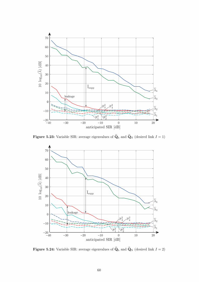
−40 −30 −20 −10 0 10 20−20

−10

0

10

20

30

40

50

60

70

anticipated SIR [dB]

Isupp

σ21 σ

22

σ23 σ

24 λ2

λ4

λ3

λ1

leakage

10log10(λ)[dB]

Figure 5.23: Variable SIR: average eigenvalues of Qb and QN (desired link I = 1)

−40 −30 −20 −10 0 10 20−20

−10

0

10

20

30

40

50

60

70

anticipated SIR [dB]

10log10(λ)[dB]

Isupp

leakage

λ2

λ4

λ3

λ1σ21 σ

22

σ23 σ

24

Figure 5.24: Variable SIR: average eigenvalues of Qb and QN (desired link I = 2)

60

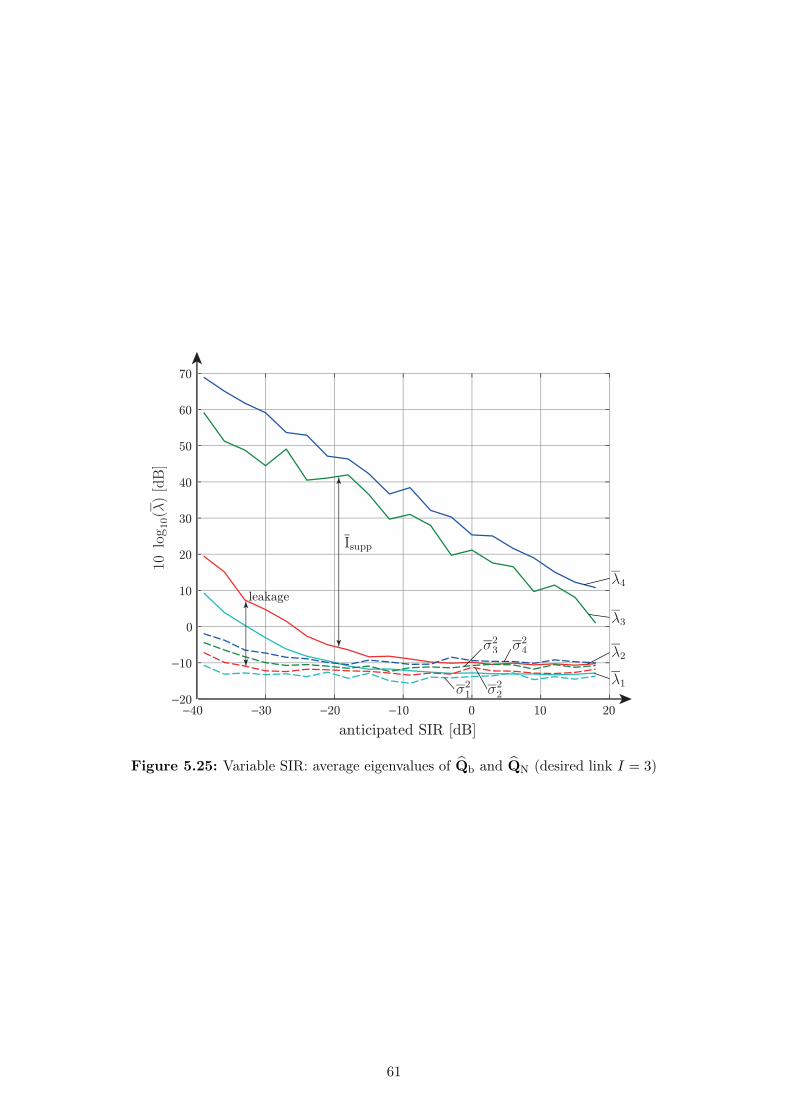
−40 −30 −20 −10 0 10 20−20

−10

0

10

20

30

40

50

60

70

anticipated SIR [dB]

10log10(λ)[dB]

λ2

λ4

λ3

λ1σ21 σ

22

σ23 σ

24

Isupp

leakage

Figure 5.25: Variable SIR: average eigenvalues of Qb and QN (desired link I = 3)

61

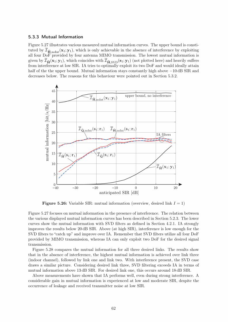
5.3.3 Mutual Information

Figure 5.27 illustrates various measured mutual information curves. The upper bound is consti-tuted by I

H,noInt(x1;y1), which is only achievable in the absence of interference by exploiting

all four DoF provided by four antenna MIMO transmission. The lowest mutual information isgiven by I

H(x1;y1), which coincides with I

H,SVD(s1;y1) (not plotted here) and heavily suffers

from interference at low SIR. IA tries to optimally exploit its two DoF and would ideally attainhalf of the the upper bound. Mutual information stays constantly high above −10 dB SIR anddecreases below. The reasons for this behaviour were pointed out in Section 5.3.2.

−40 −30 −20 −10 0 10 200

5

10

15

20

25

30

35

40

45

anticipated SIR [dB]

mutu

al info

rmat

ion [bit/s

/Hz]

IA filters

upper bound, no interferenceI bH,noInt

(x1;y1)

I bH,noInt(s1; r1)I bQ,noInt

(s1; r1)

I bQ(s1; r1)I bH

(s1; r1)

I bH(x1;y1)

Figure 5.26: Variable SIR: mutual information (overview, desired link I = 1)

Figure 5.27 focuses on mutual information in the presence of interference. The relation betweenthe various displayed mutual information curves has been described in Section 5.2.3. The lowercurves show the mutual information with SVD filters as defined in Section 4.2.1. IA stronglyimproves the results below 20 dB SIR. Above (at high SIR), interference is low enough for theSVD filters to “catch up” and improve over IA. Remember that SVD filters utilize all four DoFprovided by MIMO transmission, whereas IA can only exploit two DoF for the desired signaltransmission.

Figure 5.28 compares the mutual information for all three desired links. The results showthat in the absence of interference, the highest mutual information is achieved over link three(indoor channel), followed by link one and link two. With interference present, the SVD casedraws a similar picture. Considering desired link three, SVD filtering exceeds IA in terms ofmutual information above 13 dB SIR. For desired link one, this occurs around 18 dB SIR.

Above measurements have shown that IA performs well, even during strong interference. Aconsiderable gain in mutual information is experienced at low and moderate SIR, despite theoccurrence of leakage and received transmitter noise at low SIR.

62

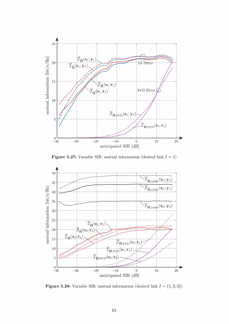
−40 −30 −20 −10 0 10 200

5

10

15

20

25

anticipated SIR [dB]

mutu

al info

rmat

ion [bit/s

/Hz]

SVD filters

IA filtersI bH

(s1;y1)

I bQ(s1;y1)

I bQ(s1; r1)

I bH(s1; r1)

I bH,SVD(s1; r1)

I bH,SVD(s1;y1)

Figure 5.27: Variable SIR: mutual information (desired link I = 1)

−40 −30 −20 −10 0 10 200

5

10

15

20

25

30

35

40

45

50

anticipated SIR [dB]

mutu

al info

rmat

ion [bit/s

/Hz]

I bH,noInt(x2;y2)

I bH,SVD(s3; r3)

I bH,SVD(s2; r2)

I bH,SVD(s1; r1)

I bH(s1; r1)

I bH(s2; r2)

I bH(s3; r3)

I bH,noInt(x1;y1)

I bH,noInt(x3;y3)

Figure 5.28: Variable SIR: mutual information (desired link I = {1, 2, 3})

63

Chapter 6

Conclusion and Outlook

Throughout this work, an interference mitigation technique for wireless multi-user networkscalled Interference Alignment (IA) was investigated and implemented on the Vienna MIMOTestbed (VMTB). Theoretical aspects such as the mathematical background and feasibilitywere discussed. The VMTB was utilized to perform a measurement based analysis. Neces-sary augmentations in hardware, software and signal generation that make IA possible weredescribed. Performance measures to investigate and compare the alignment quality were in-troduced.

The first measurement dealt with feasibility of IA at fixed SNR and SIR. It was shown, foreach of the three possible links individually, that interference is aligned at the receiver. Themutual information, representative of data rate, was thereby strongly improved. Further mea-surements investigated the impact of variable SNR and variable SIR, respectively. It was shownthat IA reaches “half the cake” in terms of data rate, namely half of the mutual informationthat could be achieved in the absence of interference. However, the results were aggravated byhardware influences such as unsuppressed transmitter noise and by outdated filters that causedleakage.

This work restricted itself to quasi-static channels with no deliberate movement (measure-ments took place at fixed receiver positions, no moving scatterers were placed intentionally).Another thesis [23] utilizes the same testbed and investigates how spatially outdated IA filtersaffect the alignment.

Many aspects of the system could be investigated in the future, the most relevant are:

• Low SNR: How does IA perform at low SNR (below 10 dB)?

- Noisy channel estimates might impair the alignment.

• Feedback: An ideal feedback link constituted by a dedicated fiber network was used.

- Limited feedback is more realistic.

- Quantized feedback is usually used and has already been investigated in theory.

• Channels: The virtual channels to the non-existing receivers are full rank and constant.

- Measured channels,

- spatially correlated channels,

- time varying channels (simulated or measured) could be investigated.

• Schemes: An efficient closed form solution for the IA filters was used.

- IA with constraints on e.g. SINR maximization is of interest.

- Iterative algorithms have been proposed in literature.

- Coordinated multipoint is a prominent alternative to IA.

64

• Implementation: A more realistic implementation could be considered.

- Frame structure according to a standard (e.g. LTE or WLAN).

To conclude this work: IA was shown to be feasible on a real world testbed. Difficulties inimplementation will arise in more realistic systems with moving receivers and moving scatterers,where the filter computation-time becomes a more pressing issue. Performing optimal feedbackand synchronization in more realistic scenarios is an open problem that is currently investigated.

The author of this work sees a possible incorporation of IA in the further progression of WLANor LTE, particularly in applications where neither the transmitters nor the receivers moveconsiderably. This mitigates the synchronization issue and the filter computation-time issue.

The thorough investigation of various IA aspects is currently subject of several research projectswhose outcome will determine the viability of IA and how it compares to competitive schemes.An efficient interference management scheme would pave the way for wireless multi-user net-works with substantially increased spectral efficiency and data throughput.Interference Alignment might be that scheme.

Martin Mayer, October 2013

65

List of Figures

1.1 Basic principle of TDMA in the three user case . . . . . . . . . . . . . . . . . . 31.2 Basic principle of IA in the three user case . . . . . . . . . . . . . . . . . . . . . 3

2.1 (4× 4, 2)3 MIMO interference channel . . . . . . . . . . . . . . . . . . . . . . . 62.2 Signal vectors in a (2× 2, 1)2 interference channel without noise . . . . . . . . . 11

3.1 Deployment of Vienna MIMO Testbed . . . . . . . . . . . . . . . . . . . . . . . 133.2 TX1 antenna setup . . . . . . . . . . . . . . . . . . . . . . . . . . . . . . . . . . 143.3 TX2 antenna setup with sensors . . . . . . . . . . . . . . . . . . . . . . . . . . . 143.4 TX3 station . . . . . . . . . . . . . . . . . . . . . . . . . . . . . . . . . . . . . . 143.5 TX3 to RX indoor channel . . . . . . . . . . . . . . . . . . . . . . . . . . . . . . 143.6 Transmitter overview [19] . . . . . . . . . . . . . . . . . . . . . . . . . . . . . . 153.7 Receiver overview [21] . . . . . . . . . . . . . . . . . . . . . . . . . . . . . . . . 163.8 RX antennas in laptop shell . . . . . . . . . . . . . . . . . . . . . . . . . . . . . 173.9 RX station . . . . . . . . . . . . . . . . . . . . . . . . . . . . . . . . . . . . . . 173.10 Two consecutive transmit frames . . . . . . . . . . . . . . . . . . . . . . . . . . 183.11 Basic transmit signal of a single transmission . . . . . . . . . . . . . . . . . . . 253.12 Compensation of propagation delays . . . . . . . . . . . . . . . . . . . . . . . . 253.13 Measurement script . . . . . . . . . . . . . . . . . . . . . . . . . . . . . . . . . . 28

4.1 Detailed frame structure . . . . . . . . . . . . . . . . . . . . . . . . . . . . . . . 32

5.1 Validation: measurement process . . . . . . . . . . . . . . . . . . . . . . . . . . 405.2 Validation: eigenvalues of Qb and QN (desired link I = 1) . . . . . . . . . . . . 425.3 Validation: eigenvalues of Qb and QN (desired link I = 2) . . . . . . . . . . . . 435.4 Validation: eigenvalues of Qb and QN (desired link I = 3) . . . . . . . . . . . . 435.5 Validation: mutual information comparison (desired link I = 1) . . . . . . . . . 445.6 Validation: mutual information comparison (desired link I = 2) . . . . . . . . . 445.7 Validation: mutual information comparison (desired link I = 3) . . . . . . . . . 455.8 Validation: receive power contributions (desired link I = 1) . . . . . . . . . . . 455.9 Validation: receive power contributions (desired link I = 2) . . . . . . . . . . . 465.10 Validation: receive power contributions (desired link I = 3) . . . . . . . . . . . 465.11 Variable SNR: measurement process . . . . . . . . . . . . . . . . . . . . . . . . 475.12 Variable SNR: measured powers . . . . . . . . . . . . . . . . . . . . . . . . . . . 485.13 Variable SNR: measured SNR and SIR . . . . . . . . . . . . . . . . . . . . . . . 505.14 Variable SNR: average interference suppression . . . . . . . . . . . . . . . . . . 515.15 Variable SNR: average eigenvalues of Qb and QN . . . . . . . . . . . . . . . . . 525.16 Variable SNR: mutual information (overview) . . . . . . . . . . . . . . . . . . . 535.17 Variable SNR: mutual information . . . . . . . . . . . . . . . . . . . . . . . . . 545.18 Variable SIR: measurement process . . . . . . . . . . . . . . . . . . . . . . . . . 555.19 Variable SIR: measured powers (desired link I = 1) . . . . . . . . . . . . . . . . 575.20 Variable SIR: measured powers (desired link I = {1, 2, 3}) . . . . . . . . . . . . 57

66

5.21 Variable SIR: measured SNR and SIR (desired link I = 1) . . . . . . . . . . . . 585.22 Variable SIR: average interference suppression (desired link I = {1, 2, 3}) . . . . 595.23 Variable SIR: average eigenvalues of Qb and QN (desired link I = 1) . . . . . . 605.24 Variable SIR: average eigenvalues of Qb and QN (desired link I = 2) . . . . . . 605.25 Variable SIR: average eigenvalues of Qb and QN (desired link I = 3) . . . . . . 615.26 Variable SIR: mutual information (overview, desired link I = 1) . . . . . . . . . 625.27 Variable SIR: mutual information (desired link I = 1) . . . . . . . . . . . . . . 635.28 Variable SIR: mutual information (desired link I = {1, 2, 3}) . . . . . . . . . . . 63

67

Bibliography

[1] Viveck R. Cadambe and Syed A. Jafar. Interference Alignment and Degrees of Freedom ofthe K-User Interference Channel. IEEE Transactions on Information Theory, 54, August2008.

[2] Omar El Ayach, Steven W Peters, and RW Heath. Real World Feasibility of InterferenceAlignment using MIMO-OFDM Channel Measurements. In Military CommunicationsConference, 2009. MILCOM 2009. IEEE, pages 1–6. IEEE, 2009.

[3] Viveck R. Cadambe Krishna Gomadam and Syed A. Jafar. Approaching the Capacity ofWireless Networks through Distributed Interference Alignment. In Global Telecommuni-cations Conference, 2008. IEEE GLOBECOM 2008. IEEE, pages 1–6. IEEE, 2008.

[4] Steven W Peters and Robert W Heath. Interference Alignment via Alternating Minimiza-tion. In Acoustics, Speech and Signal Processing, 2009. ICASSP 2009. IEEE InternationalConference on, pages 2445–2448. IEEE, 2009.

[5] Omar El Ayach, Steven W Peters, and Robert W Heath. The Feasibility of InterferenceAlignment Over Measured MIMO-OFDM Channels. Vehicular Technology, IEEE Trans-actions on, 59(9):4309–4321, 2010.

[6] O González, D Ramirez, I Santamaria, JA Garcia-Naya, and L Castedo. ExperimentalValidation of Interference Alignment Techniques using a Multiuser MIMO Testbed. InSmart Antennas (WSA), 2011 International ITG Workshop on, pages 1–8. IEEE, 2011.

[7] Roland Tresch and Maxime Guillaud. Cellular Interference Alignment with ImperfectChannel Knowledge. In Communications Workshops, 2009. ICC Workshops 2009. IEEEInternational Conference on, pages 1–5. IEEE, 2009.

[8] JA Garcıa-Naya, L Castedo, O González, D Ramırez, and I Santamaria. ExperimentalEvaluation of Interference Alignment Under Imperfect Channel State Information. Proc.EUSIPCO 2011, 2011.

[9] Per Zetterberg and Nima N Moghadam. An Experimental Investigation of SIMO, MIMO,Interference-Alignment (IA) and Coordinated Multi-Point (CoMP). In Systems, Signalsand Image Processing (IWSSIP), 2012 19th International Conference on, pages 211–216.IEEE, 2012.

[10] Martin Mayer, Gerald Artner, Gabor Hannak, Martin Lerch, and Maxime Guillaud. Mea-surement Based Evaluation of Interference Alignment on the Vienna MIMO Testbed. TheTenth International Symposium on Wireless Communication Systems (ISWCS), 2013.

[11] Emre Telatar. Capacity of Multi-antenna Gaussian Channels. European transactions ontelecommunications, 10(6):585–595, 1999.

[12] Abolfazl Sayed Motahari and Amir Keyvan Khandani. Capacity Bounds for the GaussianInterference Channel. Information Theory, IEEE Transactions on, 55(2):620–643, 2009.

68

[13] Anders Host-Madsen and Aria Nosratinia. The Multiplexing Gain of Wireless Networks.In Information Theory, 2005. ISIT 2005. Proceedings. International Symposium on, pages2065–2069. IEEE, 2005.

[14] Cenk M Yetis, Tiangao Gou, Syed A Jafar, and Ahmet H Kayran. Feasibility Conditionsfor Interference Alignment. In Global Telecommunications Conference, 2009. GLOBECOM2009. IEEE, pages 1–6. IEEE, 2009.

[15] Meisam Razaviyayn, Gennady Lyubeznik, and Zhi-Quan Luo. On the Degrees of FreedomAchievable Through Interference Alignment in a MIMO Interference Channel. SignalProcessing, IEEE Transactions on, 60(2):812–821, 2012.

[16] Gerard J Foschini and Michael J Gans. On Limits of Wireless Communications in aFading Environment when using Multiple Antennas. Wireless personal communications,6(3):311–335, 1998.

[17] Guy Bresler, Dustin Cartwright, and David Tse. Feasibility of interference alignmentfor the MIMO interference channel: the symmetric square case. In Information TheoryWorkshop (ITW), 2011 IEEE, pages 447–451. IEEE, 2011.

[18] Leonhard Edlinger. Vienna Wireless Testbed. Master’s thesis, Vienna University of Tech-nology, November 2011.

[19] Edin Huremović. Wireless Testbed Transmitter. Master’s thesis, Vienna University ofTechnology, August 2011.

[20] Armin Disslbacher-Fink. Hardware-based Timing Synchronization. Master’s thesis, Vi-enna University of Technology, December 2010.

[21] Heinz Haderer. Wireless Testbed Receiver. Master’s thesis, Vienna University of Technol-ogy, December 2011.

[22] Jaiganesh Balakrishnan, Markus Rupp, and Harish Viswanathan. Optimal Channel Train-ing for Multiple Antenna Systems. Multiaccess, mobility and teletraffic for wireless com-munications, 5:25, 2000.

[23] Gerald Artner. Receiver Location Sensitivity of Interference Alignment. Master’s thesis,Vienna University of Technology, October 2013.

69