Measurement and Simulation of Underground Heat

Collecting Processes with COMSOL MultiphysicsMartin Pies, Stepan Ozana, Radovan Hajovsky, and Petr Vojcinak

Abstract—The paper deals with analysis of temperatureprocesses within the experimental borehole located at themining dump. It consists of heat collector and measurementsystem for temperature measurement and wireless data transfer.The paper focuses on creation of 2D and 3D model of the heatcollector and the solution of heat transfer equation by use offinite element method in COMSOL Multiphysics.

Index Terms—measurement, computational modeling, miningindustry, finite element methods, data processing.

I. INTRODUCTION

THE issue of mining dumps is very extensive. The

heaps are made from waste and tailings from coal

mines. Waste rocks can catch fire spontaneously any time

and mining dump starts to burn. Temperatures can change

immediately. Fast change of temperature has a bad effect

on the environment, whether it is the fauna, flora, or the

surrounding buildings and humans. CO and CH4 arise as a

secondary product of combustion. It is dangerous for living

organisms due to exhaust fumes and high temperature that

can reach to the buildings on the ground. It is one of the main

reasons why the presented data model is being developed.

Currently we are monitoring temperature changes in the

mining dump. It is a large network made up of tens of

sensors. The sensors measure temperatures at depths of 3and 6 meters. Temperature distribution throughout the heap

is determined with using mathematical interpolated methods

based on the temperature measurements [1].

Current situation illustrated in Fig. 1 has been changed by

adding one more experimental borehole with more additional

equipments than the other borehole have at these days.

The reason of adding this experimental borehole is applied

research in the field of heat collection, it is assumed that its

results will be applied to the whole mining dump area. All of

the data, as the same as for the other sensors, is transferred

to the MySQL database by GPRS, then it is accessed and

processed by MATLAB and Simulink environment [2].

The block scheme of the measurement system which is

used for whole boreholes (both standard and experimental)

is shown in Fig. 2.

The simulation model described in this paper handles one

particular experimental borehole but it can be applied for the

entire set of all boreholes provided all necessary parameters

are predefined.

Manuscript received June 11th, 2013; revised July 25th , 2013. This workwas supported by the project of the Technology Agency of the CzechRepublic No. TA01020282 “Enhancement of quality of environment withrespect to occurrence of endogenous fires in mine dumps and industrialwaste dumps, including its modeling and spread prediction.”

All authors are with the Department of Cybernetics and BiomedicalEngineering, VSB-Technical University of Ostrava, 17. listopadu 2172/15,70833 Ostrava, Czech Republic, Europe, e-mail: martin.pies@vsb.cz.

Fig. 1. Current sensoric network with experimental borehole

Fig. 2. Block scheme of autonomous measurement system

II. MATHEMATICAL DESCRIPTION

The experimental borehole was modeled as 4-chamber

heat collector, its 2D and 3D model have been created with

the use of COMSOL Multiphysics that allows solving more

complex tasks by finite elements method [1], [3].

2D model is a basic model which is consequently trans-

ferred into 3D model by use of axial symmetry.

Nominal solution in 2D model is related to the heating

power of particular heat sources (measured in watts; param-

eter Q1 − Q5), as follows:

• parameter Qsrc and Ptot (the heat power of surrounding

waste-rock mass)

• parameter Q1 (lowest chamber, inlet)

• parameter Q2 (second chamber)

• parameter Q3 (third chamber)

• parameter Q4 (fourth chamber, outlet)

Within the solution of 2D we will consider so called

general heat source, where user-defined heat sources related

to the volume is considered as[

W · m−3]

, representing alter-

native parameters of target objects Q1 − Q5. General forms

Proceedings of the World Congress on Engineering and Computer Science 2013 Vol II WCECS 2013, 23-25 October, 2013, San Francisco, USA

ISBN: 978-988-19253-1-2 ISSN: 2078-0958 (Print); ISSN: 2078-0966 (Online)

WCECS 2013

of resulting non-homogeneous partial differential equations

(as inner heat sources are included) for heat transfer in solid

bodies are given in the following form, considering Hamilton

and Laplace operators:

• for heat source with total heat power (in watts; param-

eter Ptot)

ρ · Cp · u · ∇T =∇ (k · ∇T ) + Q

Q≡Ptot

V(1)

• for general heat source (in watts per square cubic meter;

user-defined value), parameter Qsrc

ρ · Cp · u · ∇T =∇ (k · ∇T ) + Q

Q≡Qsrc (2)

where equation’s coefficients are described in table I.

TABLE IDESCRIPTION OF THE PARAMETERS

T ≡ T (x, y, t) thermodynamictemperature (in2D model, time-dependent)

[K]

T ≡ T (x, y, z, t) thermodynamictemperature (in3D model, time-dependent)

[K]

t continuous time [s]

ρ density (in particulardomain)

[

kg · m−3]

Cp ≡ cp relative heat capac-ity of particular sub-stance

[

J · kg−1· K−1

]

u = (u1, u2, u3) velocity vector field[

m · s−1]

i = ex unit direction vector(x-coordinate)

[1]

j = ey unit direction vector(y-coordinate)

[1]

k = ez unit direction vector(z-coordinate)

[1]

∇T ≡ grad (T ) gradient of thermody-namic temperature

[

K · m−1]

∇ (∇T ) ≡ div (∇T ) divergence of thermo-dynamic temperature

[

K · m−2]

k ≡ λ ≡ κ coefficient of thermalconductivity

[

W · m−1 · K−1]

Q1 − Q4 volume heat sources[

W · m−3]

Ptot total heat power ofheat source

[W]

Q5 heat power of heatsource

[

W · m−3]

V volume of heat source[

m3]

∇ Hamilton operator(Hamiltonian)

[

m−1]

∆ ≡ ∇ · ∇ = ∇2 Laplace operator

(Laplacian)

[

m−2]

The basic scheme of 2D model, shown in Fig. 3, includes

the following items:

• location and labels of the domains in 2D model;

• heat sources - values of all positive and negative heat

power (in Watts);

• boundary condition - the value of temperature T0 (in

Kelvins) at the interface inlet tube/heat source Q1 (in

Watts);

• materials of domains - list of materials in a given 3D

model (propylene glycol, steel, sand and waste–rock);

• coordinate system - it is chosen based on 3D model

and it projects chosen slice in xz workplane, thus y-

coordinate represents the third dimension in the form

of unit length (it has no effect on nominal heat power

per particular volumes of the domains as it only formal

replace of coordinates y and z);

• other data - chosen coordinates are Cartesian and

square-biased, measured in meters.

Fig. 3. 2D model - location of the domains, their labels and materials,boundary thermodynamic temperature and chosen coordinates system (xzworkplane)

III. MEASUREMENT AND MODELING OF THE THERMAL

PROCESSES IN EXPERIMENTAL BOREHOLE

A. Physical setup

Modeling of thermal processes in experimental borehole

was carried out as four-chamber model that summarizes heat

sources into four volumes.

Fig. 4. Real experimental apparatus located in Hedvika mining dump

Fig. 4 shows the heat collector used for verification of

measured values with simulation results from COMSOL

Multiphysics. The heat collector is inserted inside experi-

mental borehole. The main purpose of this experiment is to

Proceedings of the World Congress on Engineering and Computer Science 2013 Vol II WCECS 2013, 23-25 October, 2013, San Francisco, USA

ISBN: 978-988-19253-1-2 ISSN: 2078-0958 (Print); ISSN: 2078-0966 (Online)

WCECS 2013

measure heating, resp. cooling of a small area in close sur-

roundings of the experimental borehole by use of temperature

sensors Pt100. Inside there are four interconnected chambers

with cooling media. The overall height of the apparatus is

4 meters, having its top 1 meter under the ground, which

works out 5 meters of the depth altogether. Around the

borehole itself there is a cross-cylindrical system of sensors

for temperature measurement, the distance between sensors

are 0.3 m and 0.5 m horizontally and they are located in three

levels vertically, corresponding to the centers of particular

chambers, see Fig. 5. It is supposed that temperature changes

caused by enforced cooling happen at least 100 times faster

than temperature changes caused by burning of the mining

dump.

Fig. 5. Installation of measurement system around the heat collector

Before the start of the experiment the temperature in the

borehole surroundings can be considered as constant (and can

be measured within the borehole). By control intervention the

temperature in a close surroundings of the borehole will be

affected, ant the temperature trend lines can be stored.

B. Modeling of four-chamber model in COMSOL Multi-

physics

Setting of the partial differential equation describing the

model into COMSOL Multiphysics can be seen in Fig. 6.

The created model is linear time invariant with variant

space parameters. Therefore, is not necessary to deal with

absolute values of temperature, but it is enough to compute

relative temperature differences related to initial or steady

state [4], [5].

The top and sides of the modeled object will have zero

Dirichlet boundary condition that determine the ambient

temperature, or Neumann condition computed from zero (rel-

ative) ambient temperature, simulated temperature of cooled

object and heat transfer coefficient (iteration computation).

The sequence of computation is as follows:

• setting of initial condition

• setting of Dirichlet boundary condition

• input of step change of the power Qsrc (x, y, z, t) is

brought to the system

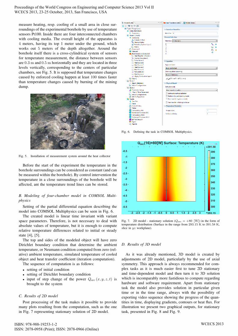
C. Results of 2D model

Post processing of the task makes it possible to provide

many plots resulting from the computation, such as the one

in Fig. 7 representing stationary solution of 2D model.

Fig. 6. Defining the task in COMSOL Multiphysics.

Fig. 7. 2D model - stationary solution (Qsrc = +80 [W]) in the form oftemperature distribution (Surface in the range from 293.15 K to 391.58 K,slice in yz workplane).

D. Results of 3D model

As it was already mentioned, 3D model is created by

adjustments of 2D model, particularly by the use of axial

symmetry. This approach is always recommended for com-

plex tasks as it is much easier first to tune 2D stationary

and time-dependent model and then turn it to 3D solution

which is incomparably more fastidious to compute regarding

hardware and software requirement. Apart from stationary

task the model also provides solution in particular given

time or in the time range, always with the possibility of

exporting video sequence showing the progress of the quan-

tities in time, displaying gradients, contours or heat flux. For

illustration we present two graphical outputs, for stationary

task, presented in Fig. 8 and Fig. 9.

Proceedings of the World Congress on Engineering and Computer Science 2013 Vol II WCECS 2013, 23-25 October, 2013, San Francisco, USA

ISBN: 978-988-19253-1-2 ISSN: 2078-0958 (Print); ISSN: 2078-0966 (Online)

WCECS 2013

Fig. 8. 3D model - stationary solution in the form of temperature field(Surface, in the range from 293.15 K to 391.17 K, orientation xyz, slicein yz workplane, its scale can be seen in lower legend).

Fig. 9. 3D model - stationary solution in the form of temperature field(Isosurface, in the range from 298.05 K to 386.27 K, orientation yz, slicein yz workplane) and total heat flow (Arrow Volume).

IV. CONCLUSION

The paper presented main idea of modeling of thermal

processes in experimental borehole at particular location.

This model can be then extended and applied for large areas

of mining dumps provided we have sufficient information

about crucial parameters of area of interest. The verification

between simulated and measured data is just in the primal

phase, but it has been proven that the concept of the model

and the methodology of experiment are valid. The most

crucial fact that has to be explored in detail in future phases

of the project is the heat source represented by the component

Qsrc (x, y, z, t), whose precise value is essential for model

results but its determination is quite a challenging issue.

The heat source Qsrc can be evaluated either in total power

per area or power per cubic meters[

W · m−3]

. Originally

the model assumes the knowledge of this parameter and

calculates the others. Further work of the project supposes

setting up of inverse task: based on measured data and their

time courses it will be possible to find the heat source Qsrc

so as the simulated data match the measured data.

This is achieved by defining the optimization task withthe use of COMSOL Livelink for MATLAB. The proposed

approach will be the objective of a patent application.

The COMSOL Multiphysics appears to be the most ap-

propriate tool for solution of such complex model due

to the fact that it allows to model nonlinear phenomena

even in heterogeneous materials with time and space variant

coefficient, while the partial differential equations are already

predefined in this environment. Of course, it lets user easily

define 1D, 2D or 3D plots with computed signals [6].

As for future work, we will mainly focus on several issues:

• Detail specification, adjustment and tuning of the pa-

rameters of the model

• Advanced validation and accordance of the model with

regard to measured data

• Creation of prediction model for the spread of under-

ground thermal processes at mining dumps based on 3D

COMSOL Multiphysics model

Within the solution of this project a unique measurement

system has been designed and implemented. The problem-

atic introduced in this paper is up-to-date with respect to

environmental policy and government interest, particularly

in the Ostravian industrial region. However, the solution can

be used and applied abroad. As a result of several surveys

in surrounding European countries, we have found similar

areas and already contacted owners and administrators of

several mining dumps regarding possible cooperation. The

computational results of the model can be also used for

determination of total calorific value (total heat power) of

such affected area and collected heat can be then used to

heating of residential areas and buildings.

REFERENCES

[1] P. Vojcinak, M. Vrtek, and R. Hajovsky, “Evaluation and monitoringof effectiveness of heat pumps via cop parameter,” in International

Conference on Circuits, Systems, Signals, 2010, pp. 240–247.[2] R. Hajovsky, S. Ozana, and P. Nevriva, “Remote sensor net for wireless

temperature and gas measurement on mining dumps,” in 7th WSEAS

International Conference on Remote Sensing (REMOTE ’11), W. Press,Ed., 2011, pp. 124–128.

[3] B. Filipova and R. Hajovsky, “Using matlab for modeling of thermalprocesses in a mining dump,” in Proceedings of the 9th IASME/WSEAS

International Conference on Heat Transfer, Thermal Engineering and

Environment, W. Press, Ed., 2011, p. 116119.[4] J. Stoer and R. Bulirsch, Introduction to Numerical Analysis. Springer

Science + Business Media, 2002.[5] L. Lixin and P. Revesz, “Interpolation methods for spatio-temporal

geographic data,” Computers, Environment and Urban Systems, vol. 28,no. 3, p. 201227, 2004.

[6] G. M. Phillips and P. J. Taylor, Theory and Applications of Numerical

Analysis. London: Elsevier Academic Press, 1996.

Proceedings of the World Congress on Engineering and Computer Science 2013 Vol II WCECS 2013, 23-25 October, 2013, San Francisco, USA

ISBN: 978-988-19253-1-2 ISSN: 2078-0958 (Print); ISSN: 2078-0966 (Online)

WCECS 2013