measurement and removal of splittings in nmr spectra by data processing

Measurement and Removal of Splittings in NMR Spectra by Data Processing J . A . JONES

Department of Chemistry, University of California. Berkeley, CA 94 720

ABSTRACT

The accurate measurement of spin-spin coupling constants is important in modern NMR Although in simple cases couplings can be measured directly from the spectrum, in general, overlap between individual lines in the mukiplet obscures the muitiplet structure and alters the apparent splitting sizes. A description of multiplets in terms of convolutions is presented, and the difficulty of performing direct deconvolution is explained Several techniques that seek to overcome these problems are described and applied to a sample mukiplet from a correlated spectroscopy spectrum. 0 1996 J o h n Wiley & Sons. Inc

INTRODUCTION

The accurate measurement of scalar coupling constants is an important problem in modern high- resolution NMR. The presence of a scalar coupling between two nuclei indicates that they are connected by one or more chemical bonds, and the size of the coupling depends on the geometry of this connection. One well-known example, described by Karplus ( I , 2), is the dependence of three-bond proton-proton coupling constants on the dihedral angle between the two proton-carbon bonds, but many other examples are known (3 ,4) .

Received October 26, 1994; revised, accepted March 20, 1995.

Current address: Merton College, Oxford OX1 4JD U.K. Telephone: +44-1865-276310; FAX +44-1865-276361; e-mail: [email protected]. Concepts in Magnetic Resonance, Vol. 8(3) 175-189 (1996) 0 1996 John Wiley & Sons, Inc. 43-7347/96/030175-15

These effects have become increasingly important for the determination of three-dimensional molec- ular structures in large molecules, especially where nuclear Overhauser effect measurements do not provide enough information to allow a complete determination.

It might seem that the problem of determining coupling constants is trivial. In a simple one- dimensional spectrum, a scalar coupling splits a line into a pair of lines, called a doublet, sepa- rated by the scalar coupling constant, J. In a two- dimensional spectrum, such as a correlated- spectroscopy (COSY) spectrum (5), the line is once again split in two, but the two components of the doublet can have opposite signs (Fig. 1). The separation between the peaks of these two lines can be measured easily from the spectrum, but this separation corresponds to the true splitting only under ideal conditions. In particular, it is possible to directly measure accurate values of J only when the splitting is much larger than the linewidth

175

176 ]ONES

(6). This is demonstrated in Fig. 2 for the case of Lorentzian lines. In general, the observed splitting (Jeff) is less than the true splitting (J), as a result of partial overlap. A similar effect occurs for the antiphase splittings that occur in COSY spectra (Fig. 2). In this case, the observed splitting is larger than the true splitting, as a result of partial cancellation.

When only a single splitting is present, it is possible to correct for this effect. For Lorentzian lines, the dependence of Jeff on J and the linewidth can be calculated analytically, and this equation can be solved to obtain J. In fact, for antiphase multiplets it is possible to correct for these effects even if the linewidth is unknown (7). This technique is difficult to apply in general and has not been widely used. When several couplings are present the situation is much more complicated. Each coupling gives rise to a splitting, resulting in multiplets that contain many lines. Each line can interfere with several others, distorting the multiplet to the extent that it is difficult to measure splittings. In the worst case it could be impossible to see the underlying multiplet structure at all.

There are many possible solutions to the problems outlined above, but they can be divided into three main groups: We can arrive at better experiments, use techniques that combine two spectra, or use single-spectrum techniques.

b- J p 4

Figure 1 Schematic multiplet from a cross-peak in a COSY spectrum. The coupling that gives rise to a particular cross-peak (the active coupling) gives rise to an antiphase doublet, with splitting J; any other couplings (passive couplings) give rise to an in-phase doublet, with splitting Jp. Every multiplet from a COSY cross- peak must contain exactly one active coupling, but can contain any number of passive couplings.

Better Experiments

It might be possible to perform a better experiment, resulting in a simpler multiplet with less overlap and interference. For example, selective decoupling can be used to remove a particular splitting from a spectrum, thus making others easier to measure. Similarly, there are many alternatives to COSY that produce simpler multiplets, such as small-flip-angle COSY (8, 9) , E.COSY (IO), z-COSY (II), P.E.COSY (22), and bilinear COSY (23). These methods can simplify the problem, but they rarely solve it completely, and appropriate data processing is still needed.

Two-Spectra Techniques

There is a group of data-processing techniques that relies on combining two spectra, acquired using different experiments, to obtain accurate values of coupling constants. Titman and Keeler have described one technique (14) that combines multiplets obtained from COSY and TOCSY spectra to measure the active coupling constant. More recently, Portilla and Freeman have developed techniques (15, 26) that use spectra obtained with and without selective decoupling. Although these techniques are useful, they are not as general as are those that require only a single spectrum, and they will not be described further.

Single-Spectrum Techniques

Finally, there are many data-processing techniques that require only a single spectrum. Some are suitable for determining the values of coupling constants and some are suitable for removing splittings from spectra; others can be used for both tasks. Perhaps the best known techniques involve curve fitting, but there are many other possibilities. These techniques are described further here.

Which approach is best? At one level the an- swer is simple: It is always better to acquire good data than to make the best of bad data, and so it is always sensible to use the best experiment available. Nevertheless, purely experimental ap- proaches are inadequate for two reasons. First, as noted above, in many cases even spectra acquired with sophisticated experiments are too complicated to analyze directly, and equally sophisticated data-processing is necessary. Second, it is sometimes necessary to analyze spectra acquired by other people, or acquired some time in the past,

MEASUREMENT AND REMOVAL OF SPLITTINGS IN SPECTRA 177

and in this case it is necessary to use the data that are available, whether they were acquired opti- mally or not. Consequently, a familiarity with data- processing techniques is useful.

It is useful to note several limitations in the discussion below. First, it is assumed that all splittings arise from weak couplings, so that the two components of a doublet have the same intensity. Multiplets arising from strong coupling, in which the doublet components have different intensities, are much more difficult to treat. Second, it will be assumed that all spectra have been phased cor- rectly, so that all the lines are in absorption phase. Finally, the techniques described below cannot generally be applied to an entire spectrum, but only to individual multiplets cut out from a’more complex spectrum. Similarly, these methods cannot be applied directly to a two-dimensional spectrum or even to a single multiplet from such a spectrum. In many cases, it is possible to modify these methods for application to a single multiplet from a two-dimensional spectrum, but it is often simpler to use traces through these multiplets. For simplicity, the word “spectrum” will be used to describe such multiplets (or traces through them, for two-dimensional multiplets) and FID (free- induction decay) will be used to describe the corresponding time-domain data obtained by Fourier transformation of the multiplet.

Figure 2 The effect of overlap on observed splittings (A) for in-phase spiittings and (B) for antiphase splittings. The individual components are plotted with a thin line; the sum and difference spectra are shown with a thicker line. The dashed lines indicate the true splitting, corresponding to the separation of the maxima of the individual components; the short solid lines indicate the observed splitting, defined as the distance between the two maxima for in-phase splittings and the distance between the maximum and minimum for antiphase splittings.

THEORY

To describe the techniques, it is first necessary to develop a language for describing the structure of a multiplet. One convenient method is to use the language of convolution, in which a multiplet is described as the convolution of several simpler structures. A basic familiarity with the properties of the Fourier transform will be assumed; several excellent texts are available at both the introduc- tory (17) and the more advanced (18, 19) levels.

Convolution

Convolution is most frequently encountered as a smoothing or blurring operation, in which a bumpy data set ( d ) is convolved with a smoothing function (w) to give a smoothed data set (s). In fact, convolution is a much more general operation that can be used to describe a variety of data manipulations. Nevertheless, smoothing is the simplest convolution to understand, and it is a good place to begin (a more detailed description can be found in Ref. 20). The simplest smoothing operation is a moving average, in which each data point is re- placed by the average of itself with several adjacent points. For example, a five-point moving average is shown in Table 1. Figure 3 is a graph of the data points. The smoothed numbers were calculated using

No smoothed values have been calculated for the points at each end of the data set; they do not have enough points on each side to allow the moving average to be calculated. There are several possible solutions to this problem. One simple and pop- ular solution is to allow the data to “wrap around,” so that the initial “7” and the final “15” are adjacent. This allows the missing points to be calculated as

and so on. In this case, the use of a wraparound results in

artifacts at the edges of the graph. The artifacts arise because the data points at the beginning of the list are very different from those at the end, and a discontinuity in the data results when a wraparound is used. As a consequence, it is important when cutting out multiplets from a spectrum to

178 JONES

Table 1

d 7 4 8 13 12 10 12 10 10 18 19 15 S 8.8 9.4 11.0 11.4 10.8 12.0 13.8 14.4

Bumpy ( d ) and Smooth (s) Data Sets'

Smoothing was achieved using a five-point moving average.

ensure that the baseline has similar intensity at each edge. compactly as

More complex smoothings can be defined that use different weightings for different points. For example, a more complex five-point smoothing can be achieved by

whenever necessary. This can be written more

s = w @ d 151

where @ indicates convolution.

Properties of Convolution Convolution has several useful properties that sim-

tive and associative, that is

si = O.ldi-2 + 0.2di-1 + 0.4di [31 + 0.24,l + O.ldi+*

This gives more weight to data points the plify calculations. First, convolution is commuta- original point. In general, any convolution can be written as

[41 a @ b = b @ a

j

w is a set of weighting values, with as many points and

as d, and all indices are allowed to wrap around (a @ b) @ c = a @ ( b @ c ) [71

* 1 I

15

* * J * * *

0 L 2

Figure 3 Bumpy and smoothed data listed in Table 1. The original bumpy data points are plotted as stars; the smoothed data are plotted as circles. Filled circles correspond to smoothed points calculated without using a wraparound; these reproduce the general upward trend of the bumpy data while removing most of the random variation. Empty circles correspond to the additional smoothed points (not listed in Table 1) calculated using a wraparound as described in Eq. [2]. In this case, using a wraparound gives rise to artifacts at the edges of the graph. These occur whenever data-points at the two ends of the list are very different, resulting in a discontinuity in the data after the wraparound.


The obvious result is that because convolutions can be expressed in any desired order, a multiplet can be described as the convolution of a singlet with a splitting pattern or as the convolution of the splitting pattern with the singlet. Second, convolution is linear, so that

a (8 (b + c) = a (8 b + a (8 c [8]

This allows convolutions to be broken up into simpler portions. Third, convolution obeys the convolution theorem, which states that

s = w (8 d = F-’(F(w) X F ( d ) ) [9]

F indicates Fourier transformation, and X indicates point-by-point multiplication. For NMR experiments, this means that convolution in the frequency domain is equivalent to multiplication in the time domain. For example, the Fourier transform of a Lorentzian line shape is a decaying exponential function, and so multiplying an FID by a decaying exponential is equivalent to convolving the corresponding spectrum with a Lorentzian line broadening.

The convolution theorem is important to us for two reasons. First, multiplication in the time domain is frequently much faster than is direct convolution in the frequency domain. Second, it is sometimes easier to understand the effects of a particular convolution when it is described in the time domain. This is even more true of the related process of deconvolution, which is described below.

More Interesting Convolutions As mentioned above, convolution is not limited to smoothing but can be used to describe a variety of manipulations. For example, convolution can be used to introduce a frequency shift, as shown in Fig. 4. Convolution of a spectrum with a “stick”

I = Figure 4 Convolution of a line at zero frequency (A) with a stick at some nonzero frequency (B) gives a line (C) at the same frequency as (B) and with the same line shape as (A). Note that in this and subsequent figures, zero frequency is at the center of the spectrum unless otherwise indicated.

(mathematically speaking, a delta function) at a particular frequency shifts the whole spectrum by an amount equal to the frequency of the stick. Similarly, convolution can be used to introduce splittings into a multiplet. This can be achieved by forming two copies of the original spectrum and shifting them in equal and opposite directions. The two copies are then added (for an in-phase doublet) or subtracted (for an antiphase doublet). Be- cause convolution is linear, the whole process can be achieved by convolving the spectrum with a single “stick doublet,” consisting of two sticks, as shown in Fig. 5. More complex splitting patterns can be achieved by convolving the result with further stick doublets, one for each splitting.

Deconvolution

Suppose you have a data set s, related to an unknown data set d by

w is a known weighting function. Deconvolution is the process of solving this equation to obtain d. Rearranging Eq. [9] gives

d = F-’(F(s) + F(w)) [111

where + indicates point-by-point division, so deconvolution in the frequency domain is equivalent to division in the time domain. If, however, any element of F(w) is equal to zero, the required division is impossible, and so deconvolution is impossible.

Another way to look at this problem is to recog- nize that the equation does not have a unique solution. Suppose d is a solution of Eq. [lo]. Now, consider a data set d’ given by

Figure 5 Convolution of a line (A) with a stick doublet (B) gives a doublet (C) with the same line shape and centered at the same frequency as (A). Note that the stick doublet is usually defined so that (C) has the same overall intensity as (A). As a result of this, the individual lines are only half as intense.

180 JONES

6 has the property that F(8) is equal to zero everywhere except at those points for which the corresponding points of F(w) are zero (so that F(w) X F(6) is zero everywhere). The corresponding convolved spectrum is

s’ = w @ d’ = F-’(F(w) X F ( d ’ ) ) [13]

As the Fourier transform is linear

F(w) X F(d’ ) = F ( w ) X F ( d ) + F(w) X F(6) ~ 4 1

and so

s’ = F-’(F(w) X F ( d ) ) = w (8 d = s [15]

Hence d and d‘ give rise to the same convolved spectrum, s. It is therefore impossible to choose between them: Both d and d’ are equally good solutions to Eq. [lo]. If any element of F(w) is equal to zero, there will be an infinite number of possible solutions, and direct deconvolution will be impossible.

Even if all of the elements of P(W) are nonzero, problems can still arise from small elements. Ex- perimental spectra are always corrupted by noise, which can be magnified by the division process. For example, Lorentzian line broadening can be deconvolved from a spectrum by dividing by a falling exponential; this has small values toward the tail of the FID, and so the noise will be ampli- fied. Deconvolution problems with this property are described as unstable.

As a result of the problems described above, direct deconvolution is frequently impractical or even completely impossible. As a consequence, many methods have been devised to perform approximate deconvolution. The methods must find some reason for choosing one of the many different possible solutions to the problem, and they must avoid excessive amplification of experimental noise. This is often described as stabilized deconvolution.

Direct Deconvolution Applied to NMR Multiplets

It is instructive to consider the application of direct deconvolution to NMR multiplets. Some properties of a multiplet can be easily deconvolved, but others, especially the splitting pattern, are much more difficult to handle. Nevertheless, it is useful

to consider why direct deconvolution fails in this case before describing other, more successful, ap- proaches.

As stated above, an NMR multiplet can be described as the convolution of four terms

multiplet = splittings 8 lineshape @frequency @ amplitude [I61

In general, it is more convenient to consider the corresponding FID, which is formed from the product of four corresponding terms. The amplitude can be described by a simple number, a, and the frequency term is a complex oscillation, ei2mr, where v is the frequency of the multiplet center in hertz. For Lorentzian line shapes, the corresponding behavior in the time domain is an exponential decay, e-”T% Hence, the time domain signal for an NMR multiplet is

m, is the Fourier transform of the splitting pattern. The subscript notation has been chosen to empha- size that the FID is recorded at discrete points in time.

The time domain signal corresponding to a doublet splitting of size J Hz is given by cos(vJt) for an in-phase splitting and by i sin(dr) for an antiphase splitting. This can be proved as follows: As described above, an in-phase splitting can be introduced by convolving the spectrum with an in-phase stick doublet, formed from two sticks, each of amplitude one-half, at frequencies +% J. The time domain signal from a stick of amplitude a and frequency u is aei2‘”‘, so the time domain signal for an inphase stick doublet is

Similarly, an antiphase splitting can be introduced by convolving the spectrum with an antiphase stick doublet, formed from a stick of amplitude minus one-half at frequency -Yd and a stick of amplitude plus one-half at frequency +%J. In this case the time domain signal is

For in-phase splittings, the sign of J is irrelevant; for antiphase splittings it determines whether the mukiplet is “down-up’’ or “up-down.’’ More complex splittings can be introduced by convolv-

MEASUREMENT AND REMOVAL OF SPLlTTlNGS IN SPECTRA 181

ing the spectrum with several stick doublets, or (equivalently) by multiplying the FID with several different cosine and sine terms.

Now that the time domain signal has been calculated, it is possible to discuss deconvolution. De- convolution of the multiplet’s amplitude is trivial; it simply corresponds to dividing each point in the FID by a; that is, to scaling the FID. Clearly, this will not affect the signal-to-noise ratio at all. De- convolution of the multiplet’s frequency is also simple; it can be achieved by dividing each point in the FID by eiZnwt or (equivalently) by multiplying each point by e-i2n”r. This corresponds to shifting the multiplet so that it is centered at zero frequency and so also will not affect the signal-to- noise ratio. Deconvolution of the line shape is, however, more complicated. As mentioned above, this is equivalent to dividing the FID by a function that becomes small near the end of the FID, and so line shape deconvolution is an unstable problem.

The problem of deconvolving spectral splittings, frequently called J-deconvolution, is generally even more difficult. Consider deconvolution of an in-phase splitting, which involves division of the FID by cos(nJt). This is equal to zero whenever Jt = n + Y2, where n is an integer, and so direct deconvolution might require dividing points in the FID by zero. In favorable cases, this will not occur because the sampling times might not coincide exactly with the zero crossings of the cosine function. In general, near zero-crossings will be suffi- cient to make the deconvolution process unstable. Nevertheless, Bothner-By and Dadok have used direct deconvolution to remove an in-phase splitting from an experimental multiplet (21). Near zero-crossings cause spikes to appear in the FID after division, and the spikes must be detected and corrected. Bothner-By and Dadok chose to identify any data points lying outside of the estimated envelope of the FID as spikes, and they reduced the spikes to smaller values. By this means the inevitable distortions were reduced to an acceptable level. However, except in unusu- ally favorable cases, this method is difficult to

Deconvolution of an antiphase splitting is even more difficult. In this case, the FID must be divided by i sin(mlt), which has zero crossings whenever Jt = n; n is an integer. As a consequence, there is always at least one zero crossing at t = 0. This point determines only the integral of the spectrum, so it is possible to adjust it by hand to give an

apply.

appropriate baseline, but this is not a very satisfactory solution.

A more elegant suggestion, proposed by Le Parco et al. (22) and by Freeman and McIntyre (23), attempts to completely avoid the zero crossings by changing the times at which data points are sampled. The method works by interpolating additional data points between each point in the FID and then resampling this data set at times well away from the zero crossings. The method is quite successful, but it gives results very similar to the simple J-doubling technique described below.

ALTERNATIVE I-DECONVOLUTION METHODS

Many methods have been developed as alternatives to direct J-deconvolution, and many of them also can be used to estimate the correct value of J by trial and error. Four methods are described in more detail below; others have been suggested (24).

J-Doubling

J-doubling, as suggested by McIntyre and Free- man (25), attempts to solve the overlap problem not by removing a splitting but by increasing the size of the splitting until the two halves of the multiplet no longer overlap. J-doubling works by use of the trigonometric identity

sin(26) = 2sin(6)cos(8) P O I Consider a multiplet from a COSY spectrum that contains just a single active (antiphase) splitting, J,, so that its time domain signal is

This can be multiplied by cos(n-J,f) to give

which corresponds to a multiplet with half the intensity and twice the active splitting.

Another way to look at J-doubling is shown in Fig. 6. Multiplying the FID by cos(.rrJt) is equivalent to convolving the spectrum with an in-phase doublet of size J. This creates an additional in- phase splitting in the multiplet, but if J is equal to J , then the two central lines exactly cancel, result-

182 ]ONES

ing in a simple antiphase doublet (this cancellation of the central lines causes the loss of half of the total intensity). When J is not equal to J, this neat cancellation does not occur, and the resulting multiplet contains additional lines.

In the simplest case (a single active coupling) doubling of the antiphase splitting is not particu- larly useful. Suppose, however, that the multiplet also contains passive splittings that are obscured as a result of partial cancellations. Doubling the antiphase splitting then acts to drag the two halves of the multiplet apart, reducing overlap and clari- fying the passive structure. If the overlap is not completely eliminated by a single doubling, then the active splitting can be doubled again: Multiply- ing Eq. [22] by cos(nU,t) gives

corresponding to a multiplet with one-quarter the intensity and four times the active splitting as ex- pected. The splitting can be doubled as many times as desired; in general n-fold doubling can be achieved by multiplying the FID by

" -1

n cos(n2" Jut) ~ 4 1 m=O

However, this process should not be repeated more often than necessary; each doubling reduces the signal-to-noise ratio by a.

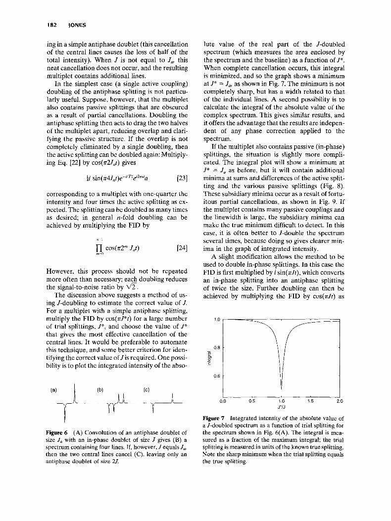
The discussion above suggests a method of using J-doubling to estimate the correct value of J. For a multiplet with a simple antiphase splitting, multiply the FID by cos(nJ*t) for a large number of trial splittings, J*, and choose the value of J* that gives the most effective cancellation of the central lines. It would be preferable to automate this technique, and some better criterion for iden- tifying the correct value of J is required. One possibility is to plot the integrated intensity of the abso-

Figure 6 (A) Convolution of an antiphase doublet of size J , with an in-phase doublet of size J gives (B) a spectrum containing four lines. If, however, J equals J, then the two central lines cancel (C), leaving only an antiphase doublet of size 21.

lute value of the real part of the J-doubled spectrum (which measures the area enclosed by the spectrum and the baseline) as a function of J*. When complete cancellation occurs, this integral is minimized, and so the graph shows a minimum at J* = J , as shown in Fig. 7. The minimum is not completely sharp, but has a width related to that of the individual lines. A second possibility is to calculate the integral of the absolute value of the complex spectrum. This gives similar results, and it offers the advantage that the results are indepen- dent of any phase correction applied to the spectrum.

If the multiplet also contains passive (in-phase) splittings, the situation is slightly more complicated. The integral plot will show a minimum at J* = Ju as before, but it will contain additional minima at sums and differences of the active splitting and the various passive splittings (Fig. 8). These subsidiary minima occur as a result of fortu- itous partial cancellations, as shown in Fig. 9. If the multiplet contains many passive couplings and the linewidth is large, the subsidiary minima can make the true minimum difficult to detect. In this case, it is often better to J-double the spectrum several times, because doing so gives clearer minima in the graph of integrated intensity.

A slight modification allows the method to be used to double in-phase splittings. In this case the FID is first multiplied by i sin(nJt), which converts an in-phase splitting into an antiphase splitting of twice the size. Further doubling can then be achieved by multiplying the FID by cos(nJt) as

0.0 0 5 1 .o 1 5 2.0 J'N

Figure 7 Integrated intensity of the absolute value of a J-doubled spectrum as a function of trial splitting for the spectrum shown in Fig. 6(A). The integral is measured as a fraction of the maximum integral; the trial splitting is measured in units of the known true splitting. Note the sharp minimum when the trial splitting equals the true splitting.


00 05 1 .o 1.5 2.0 J'IJ

Figure 8 Integrated intensity of the absolute value of a J-doubled spectrum as a function of trial splitting for the spectrum shown in Fig. 9(A). The integral is measured as a fraction of the maximum integral; the trial splitting is measured in units of the true splitting. The deep minimum at J* = J indicates the real active splitting size; the shallow minima on each side occur at sums and differences of the active and passive couplings.

before. The method also can be used to estimate J as before, but the integral plot can be badly confused by the deep subsidiary minimum which always occurs at J* = 0 (Fig. 10).

Figure 9 Spectrum (A) has a large active (antiphase) and a small passive (in-phase) splitting. J-doubling using the correct value of J gives a spectrum (B), in which all of the central lines cancel, resulting in the antiphase splitting being doubled. 1-doubling using a value of J corresponding to the difference of the active and passive couplings ( C ) or to their sum (D) results in a spectrum in which only some of the central lines cancel. This leads to the shallow minima seen in Fig. 8.

Maximum Entropy Method The maximum entropy method (MEM) is a general data-processing technique (26) applied to data from many experiments, including those in NMR (27, 28). MEM has achieved particular success in problems where direct deconvolution is unstable, which suggests that it might be useful for J- deconvolution. MEM has, in fact, been applied to the problem of J-deconvolution of spectra from electron spin resonance (29) and NMR (2430) experiments.

The application of the MEM to NMR experiments has been well described elsewhere (27,28), but the principles are easily summarized. Suppose we have an experimental FID, and we wish to determine the corresponding spectrum. Conven- tional methods (such as the Fourier transform) attempt to estimate the spectrum directly from the FID, but MEM works in the other direction.

Imagine forming the set of all possible spectra-that is, the set of spectra with every possible intensity at each frequency. This set contains an infinite number of possible spectra, but most of them can be immediately discarded. From each trial spectrum we can calculate corresponding trial data which would have been acquired using a noiseless spectrometer if the trial spectrum were in fact the true spectrum. The trial data can then be compared with the experimental data actually acquired. In most cases, the trial data will look nothing like the experimental data, so the corres-

n n I V."

0.0 0.5 1 .o 1.5 2.0 XIJ

Figure 10 Integral of the absolute value of a J-doubled spectrum as a function of trial splitting for a spectrum containing a single passive (in-phase) splitting. The integral is measured as a fraction of the maximum integral; the trial splitting is measured in units of the true splitting. The minimum at J* = J indicates the passive splitting; the minimum at a trial splitting of zero is found in all graphs of this kind for passive splittings.

184 JONES

ponding trial spectra can be discarded. The only trial spectra kept are those for which the trial data look enough like the experimental data that the difference could result from experimental noise. This can be achieved by calculating the x2 difference between the trial and experimental data and by accepting any trial spectrum for which x2 is sufficiently small.

This, however, introduces a new problem. There will in general be an infinite number of possible trial spectra for which the trial data closely match the experimental data, and it is necessary to choose among them. This choice must be made based on some prior bias about the desired solution. MEM chooses the spectrum of maximum spectral entropy, which corresponds to the “simplest” spectrum. This can be justified on the ground that any other choice would result in a spectrum more complex than the data actually require, and so the MEM choice is in some sense the safest one. For the definition of spectral entropy usually used, the resultant spectrum may not contain negative intensity, which is often a reasonable restriction.

The application of MEM to J-deconvolution of an antiphase doublet is shown in Fig. 11. Trial spectra are Fourier transformed, and the resulting trial FID is multiplied by i sin(rJt) to give trial data that are compared with the experimental data. If desired, line shape deconvolution can be achieved simultaneously by multiplying the trial data by an appropriate weighting function before com- paring them with the experimental data. This ability to perform simultaneous line shape and J- deconvolution is a major advantage of MEM.

It is, of course, possible to deconvolve in-phase splittings in much the same way: The Fourier transform of the trial spectrum is multiplied by cos(rJt) to give trial data, which are compared with the experimental data as before. The requirement that trial spectra be everywhere positive means that is is impossible to deconvolve a single in-phase splitting from a multiplet that contains both in- phase and antiphase splittings. It is, however, possible to simultaneously deconvolve an antiphase splitting and one or more in-phase splittings.

As described above, MEM can be used for J- deconvolution only if the correct value of J is known beforehand. Modifying the method to allow J to be determined is difficult. If deconvolution is attempted with a badly incorrect value of J, the iterative MEM algorithm will generally fail to converge. Although nonconvergence can be

used to rule out a range of values for J, it is not a satisfactory criterion. Furthermore, the method will converge for a range of values of J, and it is not immediately clear how to choose one value from within this range.

An extension to the method has been suggested by Delsuc and Levy (30) as a way to estimate antiphase splittings. Their method starts with many trial spectra, instead of just one. Each trial spectrum is Fourier transformed and the time domain data are multiplied by i sin(n-J*t), with a different value of J* for each spectrum. The results are then added together to form the trial data. The trial data are then matched to the experimental data as before. This results in a set of spectra which should contain the deconvolved multiplet in the spectrum corresponding to the true splitting (J* = J,) and no intensity in the other spectra that correspond to incorrect splittings. This method works reasonably well for multiplets that contain only a single antiphase splitting (30). For multiplets with additional in-phase splittings, intensity is also found in spectra corresponding to sums and differences of the antiphase and in-phase splittings. Because the false peaks completely ob- scure the desired result, the approach is impractical (24).

An implementation of MEM can be obtained from the author. The code is available free of charge for academic users\Mit is unsupported and users should have some familiarity with the C pro- gramming language. The implementation is based on a FORTRAN implementation developed by P. J. Hore and G. J. Daniel1 (31).

]-Matching Stonehouse and Keeler have recently developed a technique (32) for the measurement of splitting sizes. Because they did not name their technique, I call it J-matching. The technique was developed originally for the measurement of in-phase splittings in multiplets that contain only a single in- phase splitting; this is the simplest case to describe. If the line shape is Lorentzian, the corresponding time domain signal is

The method starts by deconvolving the multiplet frequency, to give a new time domain signal,


trial spectrum I ’

X

compare o x 2

Figure 11 J-deconvolution of an antiphase doublet using the maximum entropy method. The trial spectrum (A) is convolved with an antiphase stick doublet (B) and a lineshape function (C) to give the spectrum (D), which is Fourier transformed to give the trial data (H). In practice, it is more convenient to obtain (H) by multiplying (E), (F), and (G), the Fourier transforms of (A), (B), and (C), respectively. The trial spectrum (A) is iteratively modified to maximize its entropy (S), while simultaneously minimizing the x2 difference between the trial data (H) and the experimental data (J), which are obtained from the experimental multiplet (I) .

which corresponds to the multiplet shifted to zero frequency. This is the product of two terms, ae-t/q, which is always positive, and cos(rJt), which is oscillatory, giving a time domain signal which oscillates between positive and negative. If this signal is now multiplied by cos(rJ*t), it will in general remain oscillatory. If, however, J* = J, the signal is now

of J* which gives the smallest amount of negative intensity in the time domain signal. This technique also will work for non-Lorentzian line shapes as long as the time domain weighting corresponding to the experimental line shape is always positive.

A similar technique can be used to measure the sizes of antiphase splittings. After deconvolving the multiplet frequency, the time domain signal corresponding to an antiphase multiplet is

which is always positive. Hence, the correct value of J can be determined by seeking the value To determine J, this multiplet can be multiplied

186 JONES

by -i sin(nJ*f) for a range of values of J*. When J* = J, the time domain signal becomes

which is always positive. Hence, the correct value of J can be determined as before.

When applied to multiplets that contain only a single splitting (in-phase or antiphase), this is an excellent method for determining the splitting size. As described, however, it cannot be used to measure splittings in multiplets with more than one splitting. For example, consider a multiplet with an active (antiphase) coupling, J,, and a passive (in-phase) coupling, Jp. After deconvolution of the multiplet frequency, the corresponding time domain signal is

which contains two oscillatory terms. Any attempt to separately determine either J , or J p by J- matching will fail, because the other term will remain oscillatory. The splitting sizes can, however, be determined simultaneously by multiplying the time domain signal by -i sin(nJzt)cos(r@) and then varying both J z and J:. In the same way, if the multiplet contains three separate splittings, these must all be estimated simultaneously by varying three trial splittings. This problem makes J-matching largely impractical as a method for analyzing complex multiplets with many different splittings. A more extensive discussion can be found in Ref. 32.

Curve Fitting

Curve fitting, also called model fitting, is a well- known general technique that has been applied to many problems in NMR. It works by describing the experimental data in terms of a model with a small number of parameters; the parameters are then adjusted to make the model fit the experimental data as well as possible. For example, consider a multiplet with a single antiphase splitting. If the line shape is known to be Lorentzian, then the multiplet is described by four parameters: amplitude, frequency, linewidth, and splitting size. It is simple to calculate model data and compare them with the experimental data. If the experimental data are corrupted by noise, it will be impossible to match them exactly, so the parameters are var- ied to minimize the x2 difference between the

model and experimental data. Any general- purpose minimization routine can be used to minimize x2, and many commercial implementations are available. Most commercial NMR data-processing packages perform simple curve fitting. In some cases, they can fit the more complex patterns required for J-deconvolution. Several widely available graph-drawing programs perform curve fitting as well.

Curve fitting can be performed either directly to the time domain data, or to a spectrum obtained from them. If the spectrum is obtained by simple Fourier transformation of the time domain data then these alternatives are completely equivalent. If, however, additional data processing (such as zero filling or matched filtering) is used to obtain the spectrum, the alternatives are no longer equivalent, and it is better to fit directly to the time domain data.

Curve fitting has major advantages and disad- vantages over other methods for determining J. If the experimental data really can be accurately described by the model function used, then curve fitting is theoretically the best method for obtain- ing values for the model parameters. If, however, the model does not accurately describe the data (for example, if the experimental line shape does not match the model line shape, or if the experimental multiplet is corrupted by baseline errors) then the fitted parameters will be systematically distorted in a complicated manner. Furthermore, if the structure of the multiplet is too obscured it might not be possible to decide on an appropriate model function or on a reasonable starting position for the iterative optimization.

AN EXAMPLE

The techniques described above work well with perfect data, but it is important to investigate how well they work with genuine experimental data corrupted by noise and by line shape and baseline distortions. In some cases (for example, J- matching [32]), detailed calculations have been performed to assess the effect of these distortions on the ability of the method to extract splitting sizes, but this has not been done for all the methods described above.

Figure 12(A) shows a multiplet from the 'H COSY spectrum of isoleucine (see Fig. 13 for structure and labeling). The spectrum was obtained by conventional Fourier transform processing with zero filling and Lorentzian-to-Gaussian


resolution

0 20 40 60 80 100 0 20 40 60 80 100

I l " " " " ' 1

0 20 40 60 80 100 0 20 40 60 80 100

frequency/Hz frequency/Hz

Figure 12 (A) Multiplet from the M Q cross peak in the 'H COSY spectrum of isoleucine (see Fig. 13 for structure and labeling). (B) Part of the spectrum obtained from (A) by J- doubling five times using an active coupling constant of 13.8 Hz. Only one of the two antiphase halves is shown. (C) MEM reconstruction of the data obtained from (A) using an active coupling constant of 13.8 Hz and line shape deconvolution. The quintet in (B) is now resolved into a doublet of quartets. (D) Stick spectrum indicating the underlying structure of (A), calculated using refined coupling constants.

enhancement in both dimensions, and a cross-section through the M Q cross-peak ex- tracted. Direct analysis of this multiplet is difficult because of the low digital resolution (1.63 Hz per point) and partial cancellation between positive and negative lines arising from the antiphase M Q splitting. Additional zero filling and resolution enhancement failed to clarify the multiplet structure. The splitting pattern can, however, be determined by using the techniques described above.

The first requirement is to estimate the size of the antiphase splitting, J,. This is easily achieved by J-doubling by the McIntyre and Freeman method. Fig. 14 shows the integral of the absolute value of the J-doubled spectrum as a function of the trial coupling, J z , after doubling the antiphase splitting five times (different numbers of doublings gave similar but less clear results). The plot has a clear minimum at 13.8 Hz, indicating the size of the antiphase coupling, with shallower subsidiary minima around 7 and 22 Hz. These subsidiary minima occur at sums and differences of the active coupling constant with the average passive coupling constant (about 8 Hz).

The spectrum obtained using J-doubling with J, = 13.8 Hz and n = 5 is shown in Fig. 12(B). The resulting multiplet is a quintet, with approximate relative intensities 1:4:6:4:1, indicating the presence of four in-phase splittings, each of approxi-

mately 8 Hz. Attempts to resolve these splittings in more detail, for example by applying additional resolution enhancement to the J-doubled spectrum, were unsuccessful. This further resolution can, however, be achieved by the maximum entropy method. The result of simultaneous deconvolution of an antiphase splitting, using J , = 13.8 Hz, and line shape deconvolution is shown in Fig. 12(C). The quintet is now clearly resolved into a doublet of quartets. This is entirely consis- tent with the structure shown in Fig. 13. The antiphase splitting arises from the active coupling (IMQ = 13.8 Hz); the in-phase splittings arise from passive couplings to the adjacent methyl group (JAM = 7.6 Hz, quartet splitting) and CH group (JMx = 9.4 Hz, doublet splitting).

Now that the splitting pattern has been identi- fied, the values of the coupling constants can be refined by curve fitting directly to the original data.

CH,- CH,- CH - C -COO- I I CH, NH,'

Figure 13 Isoleucine. Italic labels refer to protons.

188 JONES

I ” ” ” ” ’ “ “ ’ “ ” ‘ 1 33 prior to its publication. Financial support was provided by the Science and Engineering Re- search Council and the North Atlantic Treaty Or- ganization.

REFERENCES

5 10 15 20 25

J,*/HZ

Figure 14 Integral of the absolute value of a J-doubled spectrum as a function of trial splitting for the spectrum shown in Fig. 12(A). The spectrum was J-doubled five times; other numbers of doublings gave similar but less clear results. Part of the graph is shown on an expanded vertical scale to emphasise the position of the minimum. The global minimum at J,* = 13.8 Hz corresponds to the active coupling; the shallower minima near 7 Hz and 22 Hz are found near the sum and difference of the active coupling and the average passive coupling (about 8 Hz).

This gives refined coupling constants of JMQ = 13.76 Hz, J A M = 7.42 Hz, and Jux = 9.40 Hz, with an estimated error of 20.1 Hz. A stick spectrum calculated using these values (Fig. 12[D]) indicates the extent of overlap and cancellation in the original multiplet.

SUMMARY

The accurate measurement of scalar coupling constants is difficult in practice because the true splitting cannot be measured from the separation between individual lines in the multiplet. Many techniques have been developed to deal with this problem, and each has advantages and disadvan- tages. If the multiplet contains a single splitting, then the J-matching technique of Stonehouse and Keeler (32) is probably best, but for more complicated multiplets it is generally necessary to use several techniques.

ACKNOWLEDGMENT

I thank P. J. Hore for introducing me to J-deconvolution and for his invaluable advice on many occasions. I also thank J. Keeler for several helpful conversations and for sending me a copy of Ref.

1. M. Karplus, “Vicinal Proton Coupling in Nuclear Magnetic Resonance,” J. Am. Chem. SOC., 1963,

2. R. K. Harris, Nuclear Magnetic Resonance Spectros- copy, Longman, Harlow, UK, 1986, p. 226.

3. V. F. Bystrov, “Spin-Spin Coupling and the Confor- mational States of Peptide Systems,” Prog. N M R Spectrosc. 1976,10, 41-81.

4. M. Eberstadt, D. F. Mierke, M. Kiick, and H. Kessler, “Peptide Conformation from Coupling Constants: Scalar Couplings as Restraints in MD Simulations,” Helv. Chim. Acta, 1992, 75, 2583- 2592.

5. D. E. Wemmer, “Homonuclear Correlated Spec- troscopy (COSY): The Basics of Two-Dimensional NMR,” Concepts Magn. Reson., 1989, 1, 59-72.

6. D. Neuhaus, G. Wagner, M. Vasak, J. H. R. Kagi, and K. Wiithrich, “Systematic Application of High- Resolution, Phase-Sensitive Two-Dimensional ‘H- NMR Techniques for the Identification of the Amino-Acid-Proton Spin Systems in Proteins,” Eur. J. Biochem., 1985,151, 257-273.

7. Y. Kimand J. H. Prestegard, “Measurement of Vici- nal Couplings from Cross Peaks in COSY Spectra,” J. M a p . Reson., 1989, 84, 9-13.

8. W. P. Aue, E. Bartholdi, and R. R. Ernst, “Two- Dimensional Spectroscopy. Application to Nuclear Magnetic Resonance,” J. Chem. Phys., 1976, 64,

9. A. Bax and R. Freeman, “Investigation of Complex Networks of Spin-Spin Coupling by Two-Dimen- sional NMR,” J. Magn. Reson., 1981, 44, 542-561.

10. C. Griesinger, 0. W. S~rensen, and R. R. Ernst, “Practical Aspects of the E.COSY Technique. Mea- surement of Scalar Spin-Spin Coupling Constants in Peptides,” J. Magn. Reson., 1987, 75, 474-492.

11. H. Oschkinat, A. Pastore, P. Pfandler, and G. Bodenhausen, “Two-Dimensional Correlation of Directly and Remotely Connected Transitions by z-Filtered COSY,” J. Magn. Reson., 1986, 69,

12. L. Mueller, “P.E.COSY, a Simple Alternative to E.COSY,” J. Magn. Reson., 1987, 72, 191-196.

13. T. Schulter-Herbriiggen, Z.L. MBdi, 0. W. Sorensen, and R. R. Ernst, “Reduction of Multiplet Complexity in COSY-Type NMR Spectra. The Bi- Iinear and Planar COSY Experiments,” Mol. Phys.,

85, 2870-2871.

2229-2246.

559-566.

1991, 72, 847-871.


14. J. J. Titman and J. Keeler, “Measurement of Homo- nuclear Coupling Constants from NMR Correlation Spectra,” J. Magn. Reson., 1990, 89, 640-646.

15. F. D. Portilla and R. Freeman, “Measurement of Spin Coupling Constants by Decoupling and Recon- volution,” J. Magn. Reson. A, 1993,104, 358-362.

16. F. D. Portilla and R. Freeman, “Accurate Determi- nation of Small Nuclear Magnetic Resonance Cou- pling Constants from Decoupling Experiments,” J. Chem. Soc. Faraday Trans., 1993,89, 4275-4278.

27. A. G. Marshall and F. R. Verdun, Fourier Trans- forms in NMR, Optical, and Mass Spectrometry, Elsevier, Amsterdam, 1990.

18. R. N. Bracewell, The Fourier Transform and its Ap- plications, 2nd ed., McGraw-Hill, New York, 1985.

19. E. 0. Brigham, The Fast Fourier Transform, Prentice-Hall, London, 1974.

20. P. A. Jansson, “Convolution and Related Con- cepts,” in Deconvolution: With Applications in Spec- troscopy, P. A. Jansson, Ed., Academic, New York,

21. A. A. Bothner-By and J. Dadok, “Useful Manipula- tions of the Free Induction Decay,”J. M a p . Reson.,

22. J-M. Le Parco, L. McIntyre, and R. Freeman, “Ac- curate Coupling Constants from Two-Dimensional Correlation Spectra by ‘JDeconvolution,’ ”1. Magn. Reson., 1991, 97, 553-567.

23. R. Freeman and L. McIntyre, “Fine Structure in NMR Correlation Spectroscopy,” Isr. J. Chem., 1992,32, 231-244.

24. J. A. Jones, D. S. Grainger, P. J. Hore, and G. J. Daniell, “Analysis of COSY Cross Peaks by Decon- volution of the Active Splittings,” J. Magn. Reson.

25. L. McIntyre and R. Freeman, “Accurate Measure- ment of Coupling Constants by J-Doubling,” J. M a p . Reson., 1992, 96, 425-431.

1984, pp. 1-34.

1987, 72, 540-543.

A, 1993, 101, 162-169.

26. S. F. Gull and G. J. Daniell, “Image Reconstruction from Incomplete and Noisy Data,” Nature (Lon- don), 1978,272, 686-690.

27. D. S. Stephenson, “Linear Prediction and Maxi- mum Entropy Methods in NMR Spectroscopy,” Prog. NMR Spectrosc., 1988,20, 515-626.

28. P. J. Hore, “Maximum Entropy and Nuclear Mag- netic Resonance,” in Maximum Entropy in Action, B. Buck and V. A. Macaulay, Eds., Clarendon, Ox- ford, 1991, pp. 41-72.

29. R. A. Jackson, “Application of the Maximum En- tropy Method to the Analysis of Electron Spin Resonance Spectra,” J. Magn. Reson., 1987, 75, 174-178.

30. M. A. Delsuc and G. C. Levy, “The Application of Maximum Entropy Processing to the Deconvolu- tion of Coupling Patterns in NMR,” J. M a p . Reson., 1988, 76, 306-315.

31. P. J. Hore and G. J. Daniell, “Maximum Entropy Reconstruction of Rotating-Frame Zeugmatogra- phy Data,” J . Magn. Reson., 1986, 69, 386-390.

32. J. Stonehouse and J. Keeler, “A Convenient and Accurate Method for the Measurement of the Val- ues of Spin-Spin Coupling Constants,” J. Magn. Reson. A, 1995,112, 43-57.

Jonathan A. Jones received a B.A. in chemistry from Oxford University in 1989. His graduate research, supervised by Peter Hore, dealt with the application of data- processing techniques to NMR spectroscopy and imaging, and he was awarded a D.Phil. in 1992. After one year of postdoctoral work with George Radda, he was elec- ted to a Junior Research Fellowship at Mer-

ton College, Oxford. This paper was produced during his tenure as an SERC-NATO postdoctoral fellow with Alexander Pines at Berkeley. His research interests include the influence of Berry’s phase on relaxation in zero-field NMR and nuclear quadrupole resonance.

measurement and removal of splittings in nmr spectra by data processing

Documents