measurement and classification of urinary … · diagnosis and monitoring of diabetes and chronic...

MEASUREMENT AND CLASSIFICATION OF URINARY DIELECTRIC PROPERTIES FOR TYPE 2 DIABETES

MELLITUS AND CHRONIC KIDNEY DISEASE

MUN PECK SHEN

FACULTY OF ENGINEERING

UNIVERSITY OF MALAYA KUALA LUMPUR

2016

MEASUREMENT AND CLASSIFICATION OF

URINARY DIELECTRIC PROPERTIES FOR TYPE 2

DIABETES MELLITUS AND CHRONIC KIDNEY

DISEASE

MUN PECK SHEN

THESIS SUBMITTED IN FULFILMENT OF THE

REQUIREMENTS FOR THE DEGREE OF DOCTOR

OF PHILOSOPHY

FACULTY OF ENGINEERING

UNIVERSITY OF MALAYA

KUALA LUMPUR

2016

UNIVERSITY OF MALAYA

ORIGINAL LITERARY WORK DECLARATION

Name of Candidate: Mun Peck Shen (I.C/Passport No: 881110-43-5850)

Registration/Matric No: KHA 120116

Name of Degree: Doctor of Philosophy

Title of Project Paper/Research Report/Dissertation/Thesis (―this Work‖):

Measurement and Classification of Urinary Dielectric Properties for Type 2

Diabetes Mellitus and Chronic Kidney Disease

Field of Study: Biomedical Engineering

I do solemnly and sincerely declare that:

(1) I am the sole author/writer of this Work;

(2) This Work is original;

(3) Any use of any work in which copyright exists was done by way of fair

dealing and for permitted purposes and any excerpt or extract from, or

reference to or reproduction of any copyright work has been disclosed

expressly and sufficiently and the title of the Work and its authorship have

been acknowledged in this Work;

(4) I do not have any actual knowledge nor do I ought reasonably to know that

the making of this work constitutes an infringement of any copyright work;

(5) I hereby assign all and every rights in the copyright to this Work to the

University of Malaya (―UM‖), who henceforth shall be owner of the

copyright in this Work and that any reproduction or use in any form or by any

means whatsoever is prohibited without the written consent of UM having

been first had and obtained;

(6) I am fully aware that if in the course of making this Work I have infringed

any copyright whether intentionally or otherwise, I may be subject to legal

action or any other action as may be determined by UM.

Candidate‘s Signature Date:

Subscribed and solemnly declared before,

Witness‘s Signature Date:

Name:

Designation:

iii

ABSTRACT

Diagnosis and monitoring of diabetes and chronic kidney disease are of crucial

importance for preventing end-stage kidney failure. The measurement of dielectric

properties has generated interest for clinical utility. In this study, the urinary dielectric

properties and behaviour of subjects with Type 2 diabetes mellitus (DM), subjects with

chronic kidney disease (CKD), and normal subjects are investigated. The measurements

were conducted using open-ended coaxial probe at microwave frequencies between 0.2

GHz and 50 GHz at room temperature (25°C), 30°C and human body temperature

(37°C), respectively. The measurement of urinary dielectric properties for DM subjects

that obtained dielectric constant increased with glycosuria level of more than 5 g/L at

low frequencies and correlated positively with glycosuria level at frequencies above 40

GHz. Loss factor correlated negatively with glycosuria level at frequencies above 15

GHz. The strongest statistically significant difference in urinary dielectric properties

was reported at room temperature (25°C) and body temperature (37°C) across different

glycosuria and proteinuria levels, respectively. Statistically significant differences were

found in the urinary dielectric properties of the CKD subjects compared to those of the

normal subjects. Urinary dielectric properties correlated positively and negatively with

proteinuria level at frequencies below and above the ―cross-over‖ frequency point,

respectively. The experimental data closely matched the single-pole Debye model. The

relaxation dispersion and relaxation time increased with the glycosuria and proteinuria

level, while decreased with the temperature. Classifications of urinary dielectric

properties were conducted using support vector machine (SVM). In two-group

classifications, the highest accuracy of 88.72% was obtained by differentiating DM

subjects from normal subjects. The highest accuracy was achieved at 67.62% for three-

group classifications. The best classification accuracies were obtained at 30°C. This

iv

study demonstrated the potential diagnostic and prognostic value of urinary dielectric

properties for Type 2 DM and CKD.

v

ABSTRAK

Diagnosis dan pemantauan penyakit kencing manis dan penyakit buah pinggang kronik

adalah penting untuk mencegah kerosakan buah pinggang peringkat akhir. Pengukuran

sifat–sifat dielektrik telah menimbulkan minat untuk utiliti klinikal. Dalam kajian ini,

sifat-sifat dielektrik air kencing untuk subjek-subjek yang berpenyakit kencing manis

jenis kedua (DM), berpenyakit buah pinggang kronik (CKD), dan normal telah disiasat.

Pengukuran telah dijalankan dengan menggunakan prob sepaksi terbuka dalam

frekuensi gelombang mikro antara 0.2 GHz dan 50 GHz dalam suhu bilik (25°C), 30°C

dan suhu badan manusia (37°C) masing-masing. Pengukuran sifat-sifat dielektrik air

kencing untuk subjek-subjek DM memperoleh pemalar dielektrik meningkat dengan

tahap glukos kencing yang melebihi 5 g/L dalam frekuensi rendah dan berkorelasi

secara positif dengan tahap-tahap glukos kencing dalam frekuensi melebihi 40 GHz.

Faktor kehilangan berkorelasi secara negatif dengan tahap-tahap glukos kencing dalam

frekuensi melebihi 15 GHz. Perbezaan statistik yang paling signifikan dalam sifat-sifat

dielektrik air kencing dilaporkan adalah dalam suhu bilik (25°C) dan suhu badan (37°C)

bagi perbezaan tahap-tahap glukos dan protein kencing masing-masing. Perbezaan

statistik yang signifikan dalam sifat-sifat dielektrik air kencing adalah antara subjek

CKD dan normal. Sifat-sifat dielektrik air kencing berkorelasi positif dan negatif

dengan tahap-tahap protein air kencing dalam frekuensi yang mengurangi dan melebihi

titk "silang" frekuensi masing-masing. Data eksperimen memadan rapat dengan model

Debye kutub tunggal. Penyebaran dan masa santaian meningkat dengan tahap-tahap

glukos dan protein air kencing masing-masing, manakala menurun dengan suhu. Sifat-

sifat dielektrik air kencing telah dikelaskan dengan menggunakan mesin vektor

sokongan (SVM). Dalam pengelasan dua kumpulan, ketepatan tertinggi sebanyak

88.72% telah diperolehi dalam membezakan subjek-subjek berpenyakit DM daripada

normal. Ketepatan tertinggi mencapai 67.62% dalam pengelasan tiga kumpulan.

vi

Ketepatan pengelasan yang terbaik telah diperolehi dalam suhu 30°C. Kajian ini

menunjukkan nilai berpotensi diagnostik and prognostik sifat-sifat dielektrik air kencing

untuk penyakit kencing manis jenis kedua dan penyakit buah pinggang kronik.

vii

ACKNOWLEDGEMENTS

I would like to express my gratitude to my supervisor, Dr. Ting Hua Nong, whose

expertise, patience and understanding, added considerably to my graduate experience. I

appreciate his vast knowledge, assistance and support for this research. Besides that, his

technical support, patient monitoring, advice and guidance in preparing reports such as

proposals, journal papers and this thesis, have enabled me able to complete my PhD

programme within the minimum period of time. I would like to thank my co-

supervisors, Assoc. Prof. Ong Teng Aik, and Dr. Chong Yip Boon for their expertise,

assistance and technical support they provided at all levels of the research.

Very special thanks to Dr. Seyed Mostafa Mirhassani for his guidance in software

programming. His patience, kindness, and assistance has enabled me to write

programming codes with minimum errors, which is a part of this research study.

I must also acknowledge the staff of the Department of Medicine for their kind help

in subjects recruitment, urine sample collection and urine sample testing. Thanks also

go to those who provided me with assistance and medical advice at times of critical

need; Dr. Wong Chew Ming, Dr. Lim Li Han, and Prof. Dr. Ng Kwan Hong. I would

also like to thank my friend, Wong Foo Nian and members in the Electromagnet Lab for

participating in the discussions and exchange of knowledge and skills which have

helped enrich my experience.

I would like to thank my family members for their support and encouragement that

have inspired me throughout my life. Lastly, I recognise that this research would not

have been possible without financial support and I express gratitude to the University of

Malaya for providing me with the Postgraduate Research Grant.

viii

TABLE OF CONTENTS

Abstract………… ........................................................................................................... iii

Abstrak……… .................................................................................................................. v

Acknowledgements .........................................................................................................vii

Table of Contents .......................................................................................................... viii

List of Figures ............................................................................................................... xiii

List of Tables ................................................................................................................... xv

List of Symbols and Abbreviations ............................................................................. xviii

List of Appendices ......................................................................................................... xix

CHAPTER 1: INTRODUCTION .................................................................................. 1

1.1 Overview .................................................................................................................. 1

1.2 Problem Statement ................................................................................................... 2

1.3 Research Objectives ................................................................................................. 4

1.4 Significance of the Study………………..……………………………..……….....5

1.5 Chapter Organisation ............................................................................................... 5

CHAPTER 2: LITERATURE REVIEW ...................................................................... 7

2.1 Review of Diagnostic and Monitoring Method for Diabetes Mellitus .................... 7

2.2 Review of Diagnostic and Monitoring Method for Chronic Kidney Disease ......... 8

2.3 Overview of Dielectric Properties ......................................................................... 11

2.3.1 Dielectrics.............................................................................................. 11

2.3.2 Dielectric Properties Theory ................................................................. 11

2.3.3 Frequency Dependence of Dielectric Properties ................................... 14

2.3.4 Temperature Dependence of Dielectric Properties ............................... 16

2.4 Review of Dielectric Properties of Solutions ........................................................ 16

ix

2.4.1 Dielectric Properties of Water ............................................................... 16

2.4.2 Dielectric Properties of Salt, Glucose and Protein Solution ................. 18

2.5 Review of Dielectric Properties of Biological Solutions ....................................... 23

2.5.1 Dielectric Properties of Blood ............................................................... 24

2.5.2 Dielectric Properties of Urine ............................................................... 25

2.5.3 Dielectric Properties of Urine for Kidney-Related Diseases ................ 26

2.6 Measurement Techniques of Dielectric Properties ................................................ 28

2.6.1 Open-ended Coaxial Probe Technique .................................................. 28

2.6.2 Resonant Cavity Perturbation Technique .............................................. 30

2.6.3 Transmission Line Technique ............................................................... 31

2.6.4 Free Space Transmission Technique ..................................................... 32

2.6.5 Comparison among Measuring Techniques .......................................... 33

2.7 Support Vector Machine Classification ................................................................. 36

2.7.1 Classification Accuracy Analysis.......................................................... 38

2.7.2 Confusion Matrix .................................................................................. 39

2.7.3 Application of Support Vector Machine ............................................... 39

2.8 Summary ................................................................................................................ 41

CHAPTER 3: THE MEASUREMENT OF URINARY DIELECTRIC

PROPERTIES OF GLYCOSURIA FOR TYPE 2 DIABETES MELLITUS ... 43

3.1 Introduction ............................................................................................................ 43

3.2 Background Study.................................................................................................. 44

3.2.1 Overview of Diabetes Mellitus ............................................................. 44

3.2.1.1 Diabetes mellitus diagnosis and monitoring ............. 45

3.2.2 Selection of Experimental Technique ................................................... 45

3.2.2.1 Theory of coaxial probe model ................................. 45

3.3 Materials and Methods........................................................................................... 48

3.3.1 Subject Recruitment .............................................................................. 48

3.3.2 Urine Collection and Storage ................................................................ 48

3.3.3 Experimental Setup and Calibration ..................................................... 48

3.3.4 Urine Measurements ............................................................................. 50

3.3.5 Data Analysis ........................................................................................ 50

x

3.3.6 Curve Fitting ......................................................................................... 51

3.4 Results ……………………………………………………………………...…….52

3.4.1 Urine Composition ................................................................................ 52

3.4.2 Reproducibility and Accuracy ............................................................... 52

3.4.3 Dielectric Properties of Glycosuria ....................................................... 57

3.4.3.1 Overview ................................................................... 57

3.4.3.2 Statistical analysis ..................................................... 60

3.4.3.3 Comparison with Debye Model ................................ 62

3.4.3.4 Classifications accuracy between glycosuria and

non-glycosuria groups ............................................... 65

3.5 Discussion .............................................................................................................. 65

3.5.1 Reproducibility and Accuracy ............................................................... 65

3.5.2 Effect of Temperature ........................................................................... 66

3.5.3 Effect of Glucose ................................................................................... 67

3.5.4 Comparison with Debye model ............................................................. 68

3.5.5 Classification across Glycosuria and Non-glycosuria Groups .............. 69

3.6 Summary ................................................................................................................ 69


PROPERTIES OF PROTEINURIA FOR CHRONIC KIDNEY DISEASE ..... 71

4.1 Introduction ............................................................................................................ 71


4.2.1 Overview of Kidney Disease................................................................. 71

4.2.1.1 Chronic kidney disease diagnosis and monitoring .... 72


4.3.1 Subject Recruitment .............................................................................. 73

4.3.2 Urine Collection and Storage ................................................................ 73

4.3.3 Urine Measurements ............................................................................. 74

4.3.4 Data Analysis ........................................................................................ 74

4.3.5 Curve Fitting ......................................................................................... 74

4.4 Results ……………………………………………………………………………75

4.4.1 Urine Composition ................................................................................ 75

xi

4.4.2 Dielectric Properties of Proteinuria ....................................................... 76

4.4.2.1 Overview ................................................................... 76

4.4.2.2 Statistical analysis ..................................................... 78

4.4.2.3 Comparison with Debye model ................................. 82

1.1.1.4 Accuracy of classifications between normal and

CKD subjects ............................................................. 85

4.5 Discussion .............................................................................................................. 85

4.5.1 Effect of Temperature ........................................................................... 85

4.5.2 Effect of Protein .................................................................................... 86

4.5.3 Comparison with Debye Model ............................................................ 87

4.5.4 Classifications between Normal and CKD Subjects ............................. 88

4.6 Summary ................................................................................................................ 88

CHAPTER 5: CLASSIFICATION OF URINARY DIELECTRIC

PROPERTIES FOR TYPE 2 DIABETES MELLITUS AND CHRONIC

KIDNEY DISEASE ................................................................................................. 90

5.1 Introduction ............................................................................................................ 90


5.2.1 Inner-Product Kernel ............................................................................. 90

5.2.2 Model Selection..................................................................................... 92


5.3.1 Data Source ........................................................................................... 93

5.3.2 Classification Model ............................................................................. 95

5.4 Results ……………………………………………………………………………95

5.4.1 Overview ............................................................................................... 95

5.4.2 Two-group Classification: DM vs Normal, DKD vs Normal and Non-

DKD vs Normal ................................................................................ 97

5.4.3 Three-group Classifications ................................................................ 101

5.4.3.1 Classification of DM vs DKD vs normal ................ 101

5.4.3.3 Classification of DM vs non-DKD vs normal ......... 104

5.4.3.5 Classification of DKD vs non-DKD vs normal....... 107

5.5 Discussion ............................................................................................................ 110

5.5.1 Effect of Temperature in Classifications ............................................. 110

xii

5.5.2 Two-group Classifications .................................................................. 110

5.5.3 Three-group Classifications ................................................................ 111

5.5.4 Comparison Accuracy between Classification Methods ..................... 111

5.6 Summary .............................................................................................................. 113

CHAPTER 6: CONCLUSIONS AND RECOMMENDATIONS ........................... 114

6.1 Conclusions .......................................................................................................... 114

6.2 Recommendations ................................................................................................ 115

References……………………………………………..…………..……………….....117

List of Publications and Papers Presented..................................................................... 128

Appendix A: Complex curve fitting program ............................................................... 132

Appendix B: Genetic algorithm .................................................................................... 135

Appendix C: SVM classification program .................................................................... 136

xiii

LIST OF FIGURES

Figure 2.1: Complex permittivity .................................................................................... 13

Figure 2.2: Cole-Cole diagram of water at 30°C (Agilent Technologies, 2005) ............ 14

Figure 2.3: Schematic of open-ended coaxial probe technique (Alabaster, 2004) ......... 30

Figure 2.4: Schematic of perturbation resonator technique (Venkatesh & Raghavan,

2005)................................................................................................................................ 31

Figure 2.5: Schematic of transmission line waveguide technique (Venkatesh &

Raghavan, 2005).............................................................................................................. 32

Figure 2.6: Schematic of free space transmission technique (Venkatesh & Raghavan,

2005)................................................................................................................................ 33

Figure 3.1: Schematic representation of the measurement set-up ................................... 49

Figure 3.2: Comparison between measured dielectric constant of distilled water and

reference data at respective temperatures of 25°C, 30°C and 37°C for frequencies

ranging from 0.2 to 50 GHz. ........................................................................................... 53

Figure 3.3: Comparison between measured loss factor of distilled water and reference

data at respective temperatures of 25°C, 30°C and 37°C for frequencies ranging from

0.2 to 50 GHz.. ................................................................................................................ 54

Figure 3.4: The comparison between measured dielectric properties of methanol with

reference data at 25°C. .................................................................................................... 56

Figure 3.5: Measured urinary dielectric constant among subject groups at 25°C........... 58

xiv

Figure 3.6: Measured urinary loss factor among subject groups at 25°C. ...................... 59

Figure 3.7: Cole-Cole diagram of experimental urinary dielectric properties data fit to

the Debye model for glycosuria subjects at 25°C ........................................................... 63

Figure 4.1: Urinary dielectric constant of normal and CKD subjects at respective

temperatures of 25°C, 30°C and 37°C for frequencies ranging from 0.2 to 50 GHz...... 77

Figure 4.2: Urinary loss factor of normal and CKD subjects at respective temperatures

of 25°C, 30°C and 37°C for frequencies ranging from 0.2 to 50 GHz.. ......................... 78

Figure 4.3: Urinary dielectric properties of different proteinuria levels at 37°C ............ 82

Figure 4.4: Cole-Cole diagram of experimental urinary dielectric properties data fit to

the Debye model for normal and CKD subjects at 37°C ................................................ 83

Figure 5.1: Architecture of SVM for non-linear classification. ...................................... 92

Figure 5.2: Comparison of mean urinary dielectric properties between subject groups.

The subject groups between (a) DKD and normal, (b) non-DKD and normal, and (c)

DKD and non-DKD at respective temperatures of 25°C (black), 30°C (red) and 37°C

(blue). .............................................................................................................................. 97

xv

LIST OF TABLES

Table 2.1: Chronic kidney disease stages and GFR .......................................................... 9

Table 2.2: Changes in dielectric constant for a range of 1M ion aqueous solution (Pethig

& Kell, 1987; Craig, 1995).............................................................................................. 20

Table 2.3: Changes in relaxation time for a range of 1M ion solution (Craig, 1995) ..... 20

Table 2.4: Comparison between different types of measuring techniques for dielectric

properties (Icier & Baysal, 2004; Komarov et al., 2005; Venkatesh & Raghavan, 2005)

......................................................................................................................................... 34

Table 2.5: Summary of inner Kernel Function ............................................................... 38

Table 2.6: Representation of confusion matrix ............................................................... 39

Table 3.1: Types of Diabetes Mellitus ............................................................................ 44

Table 3.2: Characteristics of the DM subjects. ............................................................... 52

Table 3.3: Comparison of Debye parameters of distilled water with reference data at

25°C, 30°C and 37°C ...................................................................................................... 55

Table 3.4: Comparison of Debye parameters of 0.1M salt water with reference data at

25°C, 30°C and 37°C ...................................................................................................... 56

Table 3.5: F number and p-value of urinary dielectric properties across DM subject

groups at different microwave frequencies ..................................................................... 61

Table 3.6: Significant differences in urinary dielectric properties of group-pairs .......... 62

xvi

Table 3.7: Debye dielectric parameters of different glycosuria levels at 25°C, 30°C and

37°C ................................................................................................................................. 64

Table 3.8: Classification accuracies between non-glycosuria and glycosuria groups at

25°C, 30 °C and 37°C ..................................................................................................... 65

Table 4.1: Chemical variables of normal and CKD subjects .......................................... 76

Table 4.2: Characteristics of the CKD subjects .............................................................. 76

Table 4.3: T number and p-value of urinary dielectric properties for CKD subjects in

comparison with normal at three different temperatures and different microwave

frequencies ...................................................................................................................... 79

Table 4.4: F number and p-value of urinary dielectric properties across proteinuria

levels at different microwave frequencies ....................................................................... 80

Table 4.5: Debye dielectric parameters of different proteinuria levels at 25°C, 30°C and

37°C ................................................................................................................................. 84

Table 4.6: Classification accuracies between normal and CKD subjects at 25°C, 30 °C

and 37°C .......................................................................................................................... 85

Table 5.1: Database of DM, CKD and normal subjects .................................................. 94

Table 5.2: Clinical characteristics of DM, DKD, non-DKD and normal subjects. ......... 94

Table 5.3: Classification accuracy, sensitivity and specificity between DM, DKD and

non-DKD with normal group, respectively, at 25°C ....................................................... 98


non-DKD with normal group, respectively, at 30°C ....................................................... 99

xvii


non-DKD with normal group, respectively, at 37°C ..................................................... 100

Table 5.6: Confusion matrix for the classification of urinary dielectric constant among

DM, DKD and normal group at 25°C, 30°C and 37°C ................................................. 102

Table 5.7: Confusion matrix for the classification of urinary loss factor among DM,

DKD and normal group at 25°C, 30°C and 37°C ......................................................... 103


DM, non-DKD and normal group at 25°C, 30°C and 37°C ......................................... 105

Table 5.9: Confusion matrix for the classification of urinary loss factor among DM,

non-DKD and normal group at 25°C, 30°C and 37°C .................................................. 106


DKD, non-DKD and normal group at 25°C, 30°C and 37°C. ...................................... 108

Table 5.11: Confusion matrix for the classification of urinary loss factor among DKD,

non-DKD and normal group at 25°C, 30°C and 37°C. ................................................. 109

Table 5.12: Comparison of classification accuracies between threshold and SVM

classification method for urinary dielectric constant. ................................................... 112


classification methods for urinary loss factor. .............................................................. 112

xviii

LIST OF SYMBOLS AND ABBREVIATIONS

CKD : Chronic kidney disease

C : Clearance

DM : Diabetes mellitus

DKD : Diabetic kidney disease

E-Cal : Electronic-calibration

GA : Genetic algorithm

GFR : Glomerular filtration rate

HCG : Human Chorionic gonadotropin

HbA1c : Haemoglobin A1c

IgA : Immunoglobulin A

Q : Quality

RBF : Radial basis function

RMSPE : Root mean square percentage error

SDM : Mean of standard deviation

SVM : Support vector machine

WHO : World Health Organisation

xix

LIST OF APPENDICES

Appendix A: Complex curve fitting program ……………………………….. 132

Appendix B: Genetic algorithm ……………………………………………... 135

Appendix C: SVM classification program …………………………………... 136

1

CHAPTER 1: INTRODUCTION

1.1 Overview

DM is a common public health concern. The prevalence of DM among Malaysian

adults aged 18 years and above has increased from 11.6% in 2006 to 16.6% in 2015.

Out of 19,887,000 adult population, a total of 3,303,000 patients were found to be

diagnosed with Type 2 DM in Malaysia (International Diabetes Federation, 2016). In

the United States, 29.1 million (9.3%) people in the population were diagnosed as

having diabetes in 2012, compared to 25.8 million (8.3%) in 2010 (American Diabetes

Association, 2014). However, Type 2 DM is among the most common causes of CKD.

In Malaysia, the prevalence of patients with end stage renal failure on dialysis had

increased from 325 per million population in 2001 to 762 per million population in

2009. In 2009, there were about 58% of diabetic kidney disease (DKD) patients who

diagnosed with end stage renal failure (Feisul & Azmi, 2012).

Kidney disease is classified into acute and CKD. Patients with clinical conditions

such as congestive heart failure, acute kidney disease, DM, hypertension, urinary tract

abnormalities, systemic autoimmune disorder or excessive use of known toxins develop

higher risk of getting CKD (American Diabetes Association, 1998). Urinary glucose

measurement is an essential non-invasive approach to test for DM, while urinary protein

is one of the early signs of CKD. Persistent proteinuria followed by progressive decline

of renal function (increments in serum creatinine level) are presentations of CKD and

this eventually leads to end stage renal failure (Epstein et al., 1998).

Early diagnosis and monitoring of DM and CKD are important for prevention of

further complications. As such, targeted screening and early identification are necessary.

Urine has diagnostic and prognostic values for DM and CKD, respectively. Current

clinical determination uses urinary protein excretion and estimated glomerular filtration

2

rate (eGFR) to diagnose CKD. Monitoring of urinary protein is required as standard

care in the diagnosis and prognostication of patients with CKD. However, test strips that

use colour charts to determine glycosuria or proteinuria variability are less accurate

compared to tests using numerical readouts, as the former are subjected to numerous

interference (Goldstein et al., 2004). Therefore, there is a need for a new application in

urinary measurement.

Recently, the measurement of dielectric properties has generated interest for clinical

utility. The presence of chemical compounds and biomaterials drastically affects the

chemical and physical characteristics of the viable fluid. Studies related to aqueous

solutions and biological fluids reported biomaterial dependency of dielectric changes.

For instance, the presence of glucose results in different dielectric properties of urine

(Lonappan et al., 2004; Lonappan et al., 2007a; Bassey & Cowell, 2013). The respective

variations of haematocrit, ionic salt and glucose level also affect the dielectric properties

of blood (Alison & Sheppard, 1993; Jaspard et al., 2003; Abdalla et al., 2010).

Furthermore, different types of proteins, such as amino acids, horse haemoglobin,

bovine serum albumin, and lysozyme from chicken egg solutions have different

dielectric properties compared to water. Hence, further investigation of urinary

dielectric properties could have an impact on a potentially new diagnostic method for

DM and CKD. So far, no studies have been conducted to look into the effects of protein

in urine.

1.2 Problem Statement

The drastically increasing CKD prevalence caused by Type 2 DM has become an

important health issue. Urinary measurement is an essential non-invasive approach to

test for the presence of urinary glucose and protein in DM and CKD, respectively.

3

However, the presence of limitations in the current methods has motivated the need to

propose a new technique in urinary measurement.

Recently, the measurement of dielectric properties has generated interest for clinical

utility. From the literature, dielectric properties of biological solutions have been

determined to provide informative data. The move to measure dielectric properties of

urine arose from the need to address the following problems:

i. Urinary glucose measurement is an essential non-invasive approach for

diagnosing and monitoring DM. Current test strips that use colour charts to

determine glycosuria variability are less accurate. A comparison between

urinary test strips and a laboratory biochemical analysis is always required.

Previous studies have found that urinary dielectric properties changed with

glycosuria. However, those studies were limited, as the investigations were

carried out at low frequencies with no temperature control. The differences

in urinary dielectric properties have never been statistically validated. In

addition, correlations between urinary dielectric properties and glycosuria

level have not been studied. Investigation and validation of the differences

of urinary dielectric properties at wider frequencies and different

temperatures can provide a reliable and accurate determination of urinary

dielectric properties with glycosuria.

ii. Current clinical determination uses urinary protein excretion and eGFR to

diagnose CKD. However, this requires a long laboratory determination

time. Studies have found that the progression and retardation of CKD

closely correlate with the proteinuria level. Test strips that use colour

charts to determine proteinuria variability are less accurate. Previous

studies have reported changes of dielectric properties in different protein

4

solutions. However, no study has been conducted to look into the effects

of protein in urinary dielectric properties. There is a need to investigate

and analyse the dielectric properties of urinary protein at different

temperatures and to validate the correlations between dielectric properties

and proteinuria levels.

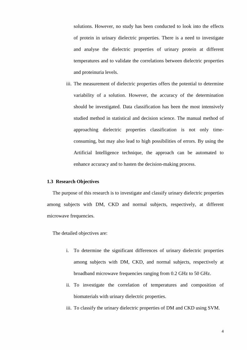
iii. The measurement of dielectric properties offers the potential to determine

variability of a solution. However, the accuracy of the determination

should be investigated. Data classification has been the most intensively

studied method in statistical and decision science. The manual method of

approaching dielectric properties classification is not only time-

consuming, but may also lead to high possibilities of errors. By using the

Artificial Intelligence technique, the approach can be automated to

enhance accuracy and to hasten the decision-making process.

1.3 Research Objectives

The purpose of this research is to investigate and classify urinary dielectric properties

among subjects with DM, CKD and normal subjects, respectively, at different

microwave frequencies.

The detailed objectives are:

i. To determine the significant differences of urinary dielectric properties

among subjects with DM, CKD, and normal subjects, respectively at

broadband microwave frequencies ranging from 0.2 GHz to 50 GHz.

ii. To investigate the correlation of temperatures and composition of

biomaterials with urinary dielectric properties.

iii. To classify the urinary dielectric properties of DM and CKD using SVM.

5

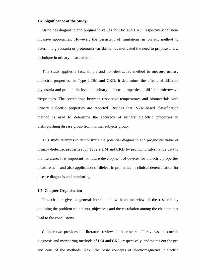
1.4 Significance of the Study

Urine has diagnostic and prognostic values for DM and CKD, respectively for non-

invasive approaches. However, the persistent of limitations in current method to

determine glycosuria or proteinuria variability has motivated the need to propose a new

technique in urinary measurement.

This study applies a fast, simple and non-destructive method to measure urinary

dielectric properties for Type 2 DM and CKD. It determines the effects of different

glycosuria and proteinuria levels in urinary dielectric properties at different microwave

frequencies. The correlations between respective temperatures and biomaterials with

urinary dielectric properties are reported. Besides that, SVM-based classification

method is used to determine the accuracy of urinary dielectric properties in

distinguishing disease group from normal subjects group.

This study attempts to demonstrate the potential diagnostic and prognostic value of

urinary dielectric properties for Type 2 DM and CKD by providing informative data to

the literature. It is important for future development of devices for dielectric properties

measurement and also application of dielectric properties in clinical determination for

disease diagnosis and monitoring.

1.5 Chapter Organisation

This chapter gives a general introduction with an overview of the research by

outlining the problem statements, objectives and the correlation among the chapters that

lead to the conclusions.

Chapter two provides the literature review of the research. It reviews the current

diagnosis and monitoring methods of DM and CKD, respectively, and points out the pro

and cons of the methods. Next, the basic concepts of electromagnetics, dielectric

6

properties and factors affecting dielectric properties are described. Then, it is followed

by reviews of the dielectric properties of water, solutions and biological fluids. A

description of the techniques of dielectric properties measurement and a comparison of

the available measurement techniques are presented. Lastly, the theories for

classification using SVM and its applications are described.

Chapter three provides a brief theoretical overview of the current diagnosis and

monitoring methods for DM. The selection of an appropriate technique for measuring

the dielectric properties of urine is described. The theories of measurement and

experimental details are explained. The experimental set up, calibration and

measurement of reference solutions are described. The reproducibility and accuracy of

the selected technique are validated. The measurement of urinary dielectric properties of

glycosuria at microwave frequencies was conducted. The experimental procedures and

data processing are described.

Chapter four reports the measurement of urinary dielectric properties of proteinuria at

microwave frequencies. A brief theoretical section provides the overview of the current

diagnosis and monitoring methods for CKD. The experimental procedures and data

processing are described.

Chapter five reports the classifications of urinary dielectric properties at microwave

frequencies. Brief explanations about the background theories of non-linear

classification and the selection of the classification model are described. Two-group and

three-group classifications are presented.

Chapter six summarises the conclusions from the previous chapters and gives

suggestions for future possibilities.

7

CHAPTER 2: LITERATURE REVIEW

2.1 Review of Diagnostic and Monitoring Method for Diabetes Mellitus

The gold standard for diagnosis of DM is the measurement of glucose concentration

in blood plasma (hyperglycaemia) due to the dysfunction of carbohydrate metabolism

that results in metabolic derangement. The World Health Organization (WHO) has

recommended a set of diagnostic criteria comprised of: Haemoglobin (Hb) A1c > 6.5%

(48 mmol/mol), fasting plasma glucose > 7.0 mmol/L (126 mg/dL), 2 h postload

glucose concentration > 11.1 mmol/L (200 mg/dL) during an oral glucose tolerance test

or symptoms of DM and casual plasma glucose concentration > 11.1 mmol/L (200

mg/dL). Repeat testing on the following day is necessary to establish the diagnosis if

any of the criteria is met by a patient. Testing to detect Type 2 DM is recommended for

all asymptomatic people who are above the age of 45 years or for those at high risk of

getting DM. Routine measurement of plasma glucose concentrations in an accredited

laboratory is not recommended as the primary method of monitoring outpatients with

DM. Laboratory glucose testing is used as a supplementary method to confirm the

accuracy of self-monitoring (Sacks et al., 2011). Portable glucose meters are

recommended to be used by individuals with DM for self-monitoring of blood glucose

concentrations due to its ease of use, convenience and accessibility. Self-monitoring is

useful for detecting asymptomatic hypoglycaemia or to avoid hyperglycaemia in

patients. However, the use of glucose meters generates high possibilities of false

positives or false negatives due to certain factors such as haematocrit level (Tang et al.,

2000), altitude, environmental temperature or humidity, hypotension, hypoxia and high

triglyceride concentrations (American Diabetes Association, 1994).

In laboratory glucose testing, overnight fasting blood (with no caloric intake for a

minimum of 8 hours) is drawn in the morning for measurement. Loss of glucose from

the sample due to glycolysis is dependent on the glucose concentration, leukocyte and

8

temperature (Ladenson et al., 1980). Fluoride, which is used as a glycolysis inhibitor, is

unable to prevent short-term glycolysis. Glucose concentration was found to decrease

for up to 4 hours after sample collection, with or without the presence of fluoride. The

glucose concentration in blood with fluoride remains stable for 72 hours at room

temperature, but the rate of glycolysis increases if the concentration of leukocyte is high

(Chan et al., 1989). Measurement of the concentration of glucose in plasma is highly

recommended because plasma can be centrifuged to avoid glycolysis without waiting

for the blood to clot (World Health Organization, 2006; American Diabetes Association,

2010). Fasting plasma glucose concentration was found to increase with age, starting

with middle age, due to homeostasis and visceral obesity that decreases glucose

tolerance (Pekkanen et al., 1999; Imbeault et al., 2003).

Semiquantitative urinary glucose testing is used only for patients who refuse or are

unable to go for blood glucose testing due to the fact that it does not reflect plasma

glucose accurately (Goldstein et al., 2004). However, it is essential for diagnosing and

monitoring DM as a non-invasive approach. It is applicable for situations where blood

glucose testing is inaccessible or unaffordable. Diabetes test strips that use oxidase

reaction to show glycosuria variability is subject to numerous interference such as drugs

and non-glucose sugars (Goldstein et al., 2004).

2.2 Review of Diagnostic and Monitoring Method for Chronic Kidney Disease

CKD is defined as the abnormalities of kidney function that present consistently for

more than 3 months. The diagnosis of CKD facilitates the disease classifications.

Currently, glomerular filtration rate (GFR) is used as the gold standard to evaluate renal

function. Patients with assessed estimated GFR (eGFR) < 90 ml/min/1.73m2 is

diagnosed as having CKD. Clinical determination to classify the disease stages based on

eGFR to diagnose overall kidney function is described in Table 2.1:

9

Table 2.1: Chronic kidney disease stages and GFR

Stage Details GFR (ml/min/1.73m2)

1 Kidney damage with normal GFR

but protein found in urine

>90

2 Kidney damage with mild decrease

in GFR

60 to 90

3 Moderate decrease in GFR 30 to 59

4 Severe reduction in GFR 15 to 29

5 Kidney failure < 15

GFR is based on Clearance, (C) where the rate of an indicator substance being

removed from plasma is measured per unit concentration. It specifies the volume of the

substance that is removed per unit of time. For example, substance Z is cleared by renal

elimination:

2.1

10

Where Uz is urinary concentration of Z, Pz is plasma concentration of Z, and V is urine

flow rate. Z refers to the creatinine of measured plasma. Concentration of serum

creatinine is affected by factors such as gender, age, ethnicity, medication, muscle mass

and protein intake (Lascano & Poggio, 2010). Furthermore, CKD seldom shows clinical

symptoms in the early stage as serum creatinine will rise only after the reduction of

renal function by at least 50% (Salifu, 2015).

Ultrasound is used to image the renal tract in patients with CKD. It is able to identify

renal size and symmetry, renal scarring, uropathy and polycystic disease in a CKD

patient. The test is conducted when a renal biopsy is required, when there is persistent

haematuria or when a rapid deterioration of renal function is observed (Bush Jr et al.,

2000).

Meanwhile, urinary protein has been shown to have diagnostic and prognostic value

for CKD. Initial pathophysiological changes in kidneys showed significant changes in

urinary proteins, which are potential biomarkers of early stage of CKD (Zürbig et al.,

2009). Urinary albumin is the most common type of protein present in urine that is

associated with CKD. Ghiggeri et al. (1985) found that protein increases in urine with

respect to the stages of CKD. Urinary protein excretion is a modifiable risk factor for

CKD progression. The progression and retardation of CKD is closely correlated with

proteinuria (Jafar et al., 2001; Atkins et al., 2005; Lea et al., 2005). However, qualitative

tests, such as chemical test strips, are subjected to numerous interference factors and are

unable to detect small amounts of albuminuria. Hence, results always need to be

confirmed with quantitative laboratory tests (Sacks et al., 2011). Monitoring of urinary

protein is certainly important as standard care for patients with CKD or those at high

risk of developing CKD.

11

2.3 Overview of Dielectric Properties

2.3.1 Dielectrics

Dielectrics are materials that allow the propagation of electromagnetic waves, which

are dependent on their electrical parameters. When potential difference is applied across

a material, it results in an electric field. Dielectric materials have virtual energy that is

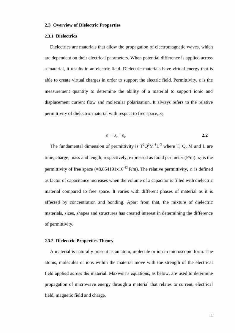
able to create virtual charges in order to support the electric field. Permittivity, is the

measurement quantity to determine the ability of a material to support ionic and

displacement current flow and molecular polarisation. It always refers to the relative

permittivity of dielectric material with respect to free space, 0.

2.2

The fundamental dimension of permittivity is T2Q

2M

-1L

-3 where T, Q, M and L are

time, charge, mass and length, respectively, expressed as farad per meter (F/m). is the

permittivity of free space (=8.854191x10-12

F/m). The relative permittivity, r is defined

as factor of capacitance increases when the volume of a capacitor is filled with dielectric

material compared to free space. It varies with different phases of material as it is

affected by concentration and bonding. Apart from that, the mixture of dielectric

materials, sizes, shapes and structures has created interest in determining the difference

of permittivity.

2.3.2 Dielectric Properties Theory

A material is naturally present as an atom, molecule or ion in microscopic form. The

atoms, molecules or ions within the material move with the strength of the electrical

field applied across the material. Maxwell‘s equations, as below, are used to determine

propagation of microwave energy through a material that relates to current, electrical

field, magnetic field and charge.

12

2.3

2.4

2.5

2.6

where E, D, H, B, are electrical field intensity, electrical flux density, magnetic

intensity field, magnetic flux density, and charge density, respectively. Faraday‘s and

Ampere‘s Law are applied to constitutive relations with Maxwell‘s equations. From the

equations shown below, the respective electrical flux density and current density vary

linearly with electrical field intensity whereas magnetic flux density is directly

proportional to magnetic field intensity.

2.7

2.8

2.9

Where J is current density, ε is permittivity, µ is permeability and σ is conductivity.

They are the constant of proportionality. Most materials exist in at least one of the

electrical dipoles, where the molecule charges are imbalanced (eg. water), the opposing

ions are charged (eg. salt) or the atom nucleus is separated from its electron cloud.

When the electrical field is applied, the dipoles rotate to align within the field in the

correct polarity. Permittivity describes dielectric properties that influence the reflection

of electromagnetic waves at interfaces and the attenuation of wave energy within

materials. Dielectric properties of materials can be defined in terms of their relative

permittivity, r. Relative permittivity is represented as a complex quantity in terms of

13

real (r’)and imaginary r

’’) parts that are referred to as dielectric constant and loss

factor, respectively, as follows:

2.10

Where r’ is the energy stored and r

’’ is the energy lost when exposed to an electrical

field. The real and imaginary parts may be described as 90° out of phase (Figure 2.1).

Figure 2.1: Complex permittivity

Loss tangent is defined as the ratio of the imaginary part to the real part:

2.11

Loss tangent is the mechanism that causes dielectric loss in heterogenous mixtures

that include electronic, polar, atomic and Maxwell-Wagner responses (Metaxas &

Meredith, 1983). However, ionic conductance and dipole rotation are the dominant loss

mechanisms at microwave frequencies (Ryynänen, 1995). Complex permittivity can

also be expressed on the Cole-Cole diagram where r’’ is plotted against r

’. Figure 2.2

shows the Cole-Cole diagram of pure water at 30°C. Infinite or high frequency relative

permittivity, ε∞ and static or zero-frequency relative permittivity, εs can be obtained

from the intersecting points on the x-axis, respectively. Dielectric lossy materials

convert electrical energy into heat in the presence of microwave frequencies that

14

increase temperature. The increase of temperature is directly proportional to loss factor

(Nelson, 1996).

Figure 2.2: Cole-Cole diagram of water at 30°C (Agilent Technologies, 2005)

2.3.3 Frequency Dependence of Dielectric Properties

Dielectric properties are frequency dependent. For moist dielectric materials, ionic

conductivity is dominant at frequencies lower than 200 MHz. Ionic conductivity and

free water dipole rotation are combined to take part at microwave frequencies.

Maximum loss factor at a relaxation frequency (fc) relates to relaxation time (

).

Relaxation time is the time required for dipoles to fully orientate in an electrical field.

Debye model describes the wideband frequency dependence of the dielectric

relaxation response of liquids. Equation 2.12 below shows the single-pole Debye

equation (Pethig & Kell, 1987).

( )

2.12

where ε(ω) is the dielectric properties and ω is the angular frequency. εs is the static

relative permittivity, ε∞ is the infinite relative permittivity and η is the relaxation time of

15

the material. Generally, larger molecules have longer relaxation time (Komarov et al.,

2005). The model is further expanded to include a static conductivity, σs. This indicates

that the currents flow at infinite time due to the movement of ions in a constant field

(limiting low frequencies).

2.13

After including Equation 2.13 into Equation 2.12, the resulting equation is as below:

( )

2.14

Since

2.15

Hence,

( )

,

( )

-

2.16

For two or more relaxations, multi-pole Debye model is applied.

( )

2.17

Cole and Cole (1942) modified the Debye model into the Cole-Cole equation as

follows, with α for the distribution of relaxation time.

( )

( )

2.18

16

α ~ 0 for water and wet tissue at microwave frequencies. Maxwell-Wagner theory is

used to describe dielectric properties of mixtures and tissues, but it is only appropriate

for low microwave frequencies (Pethig & Kell, 1987).

2.3.4 Temperature Dependence of Dielectric Properties

Temperature has a significant effect on dielectric properties. For moist materials,

ionic conductance increases with temperature, resulting in loss factor increases at low

frequencies (<200 MHz) while decreases at high frequencies due to free-water

dispersion. Debye explained that viscosity reduces with temperature due to the

randomised Brownian movement of molecules. As a result, relaxation time and

dielectric constant of pure water decrease with temperature. Combination effects of

mechanisms in multi-dispersion materials show the gradual transition of dielectric

properties with respect to frequencies (Komarov et al., 2005).

2.4 Review of Dielectric Properties of Solutions

2.4.1 Dielectric Properties of Water

A water molecule consists of one oxygen and two hydrogen atoms. The hydrogen

atoms of the molecule is more often present as positive than the oxygen atom due to

hydrogen‘s bonding mechanism that results in net polarity. Interaction and orientation

of relevant molecules show how the liquid responds to electromagnetic fields. The

dielectric properties of liquids have been well established over the century. A review

was conducted by Uematsu and Franck (1980) before the 1980s, on the data regarding

static relative permittivity of water and steam by considering the physical variations.

They documented and compared the static relative permittivity of water and steam in

atmospheric pressure up to 500 MPa and between 0°C and 550°C. From the data

obtained, they discovered a new international formulation for static dielectric constant

of water and steam. Kaatze (1989) investigated the temperature and frequency

17

dependence of the dielectric properties of water. He reported that one discrete relaxation

time was found in the dielectric properties of water, using the Debye relaxation function

at microwave frequency from 1.1 to 57 GHz as well as temperature between -4.1°C and

60°C. Johri and Roberts (1990) employed a resonant microwave cavity to investigate

the dielectric response of water. They proposed the Cole-Cole response for the

behaviour of water with increased relaxation time at broader frequency ranges. Higher

order of water transitions at temperature variations were due to the nonlinear behaviour

of hydrogen bonding dipolar molecules and dipoles (Johri & Roberts, 1990). Robert et

al. (1993) continued investigating the dielectric responses of water in ice, liquid and

vapour forms. They reported various impure states of water with ions affecting the

dielectric response and that water molecules displaying temperature transition changed

with dielectric properties as the structure changed. Dielectric relaxation of water was

found to change with temperature from 0 to 100°C (Robert et al., 1993).

Fernández et al. (1995) further reviewed the static dielectric constant of water and

steam up to 600°C and 1189 MPa. The dielectric behaviours of water were evaluated

based on difference measurement techniques, frequency dependence and source of

error. Overall, at a temperature of about 25°C, the static dielectric constant of water was

reported to experience small decreases at frequencies below 1 GHz and strong decreases

at frequencies up to 40 GHz respectively. Relaxation time was decreased with

increasing temperature. However, the different techniques proposed contributed

increased discrepancies of data (Fernández et al., 1995).

In a comparison between the dielectric behaviour of water vapour and organic

liquids, Raveendranath and Mathew (1996) reported that the dielectric properties of

water vapour was higher than that of methanol and chloroform vapour. The dielectric

properties of vapours increased with temperature, unlike that of liquids. This could be

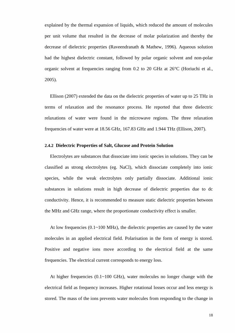
18

explained by the thermal expansion of liquids, which reduced the amount of molecules

per unit volume that resulted in the decrease of molar polarization and thereby the

decrease of dielectric properties (Raveendranath & Mathew, 1996). Aqueous solution

had the highest dielectric constant, followed by polar organic solvent and non-polar

organic solvent at frequencies ranging from 0.2 to 20 GHz at 26°C (Horiuchi et al.,

2005).

Ellison (2007) extended the data on the dielectric properties of water up to 25 THz in

terms of relaxation and the resonance process. He reported that three dielectric

relaxations of water were found in the microwave regions. The three relaxation

frequencies of water were at 18.56 GHz, 167.83 GHz and 1.944 THz (Ellison, 2007).

2.4.2 Dielectric Properties of Salt, Glucose and Protein Solution

Electrolytes are substances that dissociate into ionic species in solutions. They can be

classified as strong electrolytes (eg. NaCl), which dissociate completely into ionic

species, while the weak electrolytes only partially dissociate. Additional ionic

substances in solutions result in high decrease of dielectric properties due to dc

conductivity. Hence, it is recommended to measure static dielectric properties between

the MHz and GHz range, where the proportionate conductivity effect is smaller.

At low frequencies (0.1~100 MHz), the dielectric properties are caused by the water

molecules in an applied electrical field. Polarisation in the form of energy is stored.

Positive and negative ions move according to the electrical field at the same

frequencies. The electrical current corresponds to energy loss.

At higher frequencies (0.1~100 GHz), water molecules no longer change with the

electrical field as frequency increases. Higher rotational losses occur and less energy is

stored. The mass of the ions prevents water molecules from responding to the change in

19

the electrical field. At frequencies higher than 100 GHz, water molecules are stretched

or even pulled apart.

The decrement of dielectric constant in electrolyte solutions due to the presence of

polar ions orientate the water molecules in the solution, reducing the ability of water

molecules to re-orientate to the applied electrical field (Craig, 1995). The relationship

between the concentration of electrolytes and static dielectric constant is assumed to be

linear at the limit between 0.1 mol/l and 1 mol/l, as given by the equation below:

2.19

Where ss and sw are the static dielectric constants of sample and water respectively,

δc is the dielectric decrement that relates to concentration, c of the solute. As the

concentration of electrolytes increases, deficit of water molecules redistribute to form

ions hydration layers. Hence, the relationship between the static dielectric constant and

the concentration of ions is non-linear at higher concentration. The relaxation time also

decreases linearly with low levels of electrolyte concentration. The suggested

mechanism is due to the breaking effect of hydrogen bonding with the addition of ions

(Craig, 1995). Table 2.2 and 2.3 show the changes in dielectric constant and relaxation

time for a range of 1M ion aqueous solution.

20

Table 2.2: Changes in dielectric constant for a range of 1M ion aqueous

solution (Pethig & Kell, 1987; Craig, 1995)

Table 2.3: Changes in relaxation time for a range of 1M ion solution (Craig,

1995)

Cation ∆εr’ (±1) Anion ∆εr’ (±1)

H+

-17 F-

-5

Li+

-11 Cl-

-3

Na+

-8 I-

-7

K+

-8 OH-

-13

Rb+

-7 SO42-

-7

Mg+ -24

Ba2+

-22

La3+

-35

Cation

∆τ (ps/mol) Anion

∆τ (ps/mol)

H+

1.3 F-

-1.3

Li+

-1.0 Cl-

-1.3

Na+

-1.3 I-

-5.0

K+

-1.3 OH-

-0.7

Rb+

-1.7

Mg+ -1.3

Ba2+

-3.0

La3+

-5.0

21

Besides salt, the presence of glucose also drastically affects the chemical and

physical characters of the viable fluid. The dielectric properties of a glucose solution

were investigated by Höchtl et al. (2000). They reported that the dielectric constant

decreased while loss factor increased with respect to the glucose concentration solution

at particular 2.45 GHz. The temperature effect (25°C to 85°C) of glucose solutions in

dielectric properties was determined by Liao et al. (2001). The dielectric constant of the

glucose solution increased while the loss factor decreased with temperature,

respectively. They discovered that the dielectric properties of supersaturated glucose

were independent of concentration at a particular concentration range of about 45~56%.

Meriakri et al. (2007b) observed that glucose in solution up to 5% showed a decrease in

dielectric properties, compared to water, except for frequencies from 92 to 93 GHz

which showed slight increase of loss factor with concentration. Kim et al. (2009)

investigated the interaction of the electromagnetic field with glucose and NaCl aqueous

solutions. They reported that increasing the respective glucose and NaCl concentrations

in the solutions yielded decreased intensity of microwave reflection coefficient, S11.

Good linear dependency between relative dielectric properties and reflection coefficient,

S11 was found with increments in glucose concentration and temperature (Kim et al.,

2009). Bassey and Cowell (2013) proposed the potential usefulness of dielectric

properties to monitor the glucose level of diabetics after measuring diabetic urine with

0.1 to 1 M of urinary glucose concentration between 100 and 300 MHz at room

temperature. Smulders et al. (2013) discovered that the changes to the dielectric

properties in glucose solution were different compared to the changes in glucose

solution with 0.9% NaCl salt. They found that the presence of salt in biological

solutions could affect the sensitivity of dielectric properties of the glucose

concentration. The presence of 0.9% NaCl salt in glucose solution as a representative of

biological solution caused dielectric constant to decrease at frequencies below 20 GHz

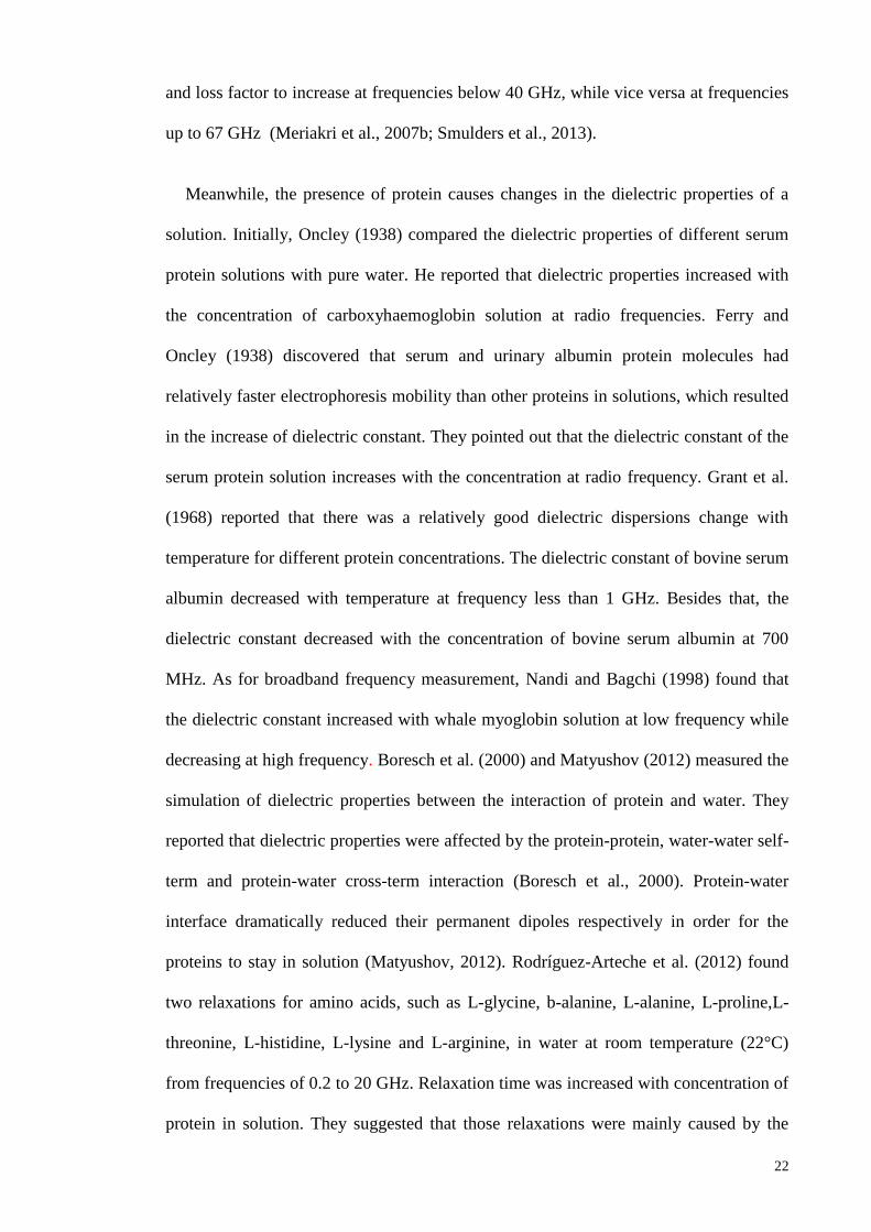
22

and loss factor to increase at frequencies below 40 GHz, while vice versa at frequencies

up to 67 GHz (Meriakri et al., 2007b; Smulders et al., 2013).

Meanwhile, the presence of protein causes changes in the dielectric properties of a

solution. Initially, Oncley (1938) compared the dielectric properties of different serum

protein solutions with pure water. He reported that dielectric properties increased with

the concentration of carboxyhaemoglobin solution at radio frequencies. Ferry and

Oncley (1938) discovered that serum and urinary albumin protein molecules had

relatively faster electrophoresis mobility than other proteins in solutions, which resulted

in the increase of dielectric constant. They pointed out that the dielectric constant of the

serum protein solution increases with the concentration at radio frequency. Grant et al.

(1968) reported that there was a relatively good dielectric dispersions change with

temperature for different protein concentrations. The dielectric constant of bovine serum

albumin decreased with temperature at frequency less than 1 GHz. Besides that, the

dielectric constant decreased with the concentration of bovine serum albumin at 700

MHz. As for broadband frequency measurement, Nandi and Bagchi (1998) found that

the dielectric constant increased with whale myoglobin solution at low frequency while

decreasing at high frequency. Boresch et al. (2000) and Matyushov (2012) measured the

simulation of dielectric properties between the interaction of protein and water. They

reported that dielectric properties were affected by the protein-protein, water-water self-

term and protein-water cross-term interaction (Boresch et al., 2000). Protein-water

interface dramatically reduced their permanent dipoles respectively in order for the

proteins to stay in solution (Matyushov, 2012). Rodríguez-Arteche et al. (2012) found

two relaxations for amino acids, such as L-glycine, b-alanine, L-alanine, L-proline,L-

threonine, L-histidine, L-lysine and L-arginine, in water at room temperature (22°C)

from frequencies of 0.2 to 20 GHz. Relaxation time was increased with concentration of

protein in solution. They suggested that those relaxations were mainly caused by the

23

rotation of amino acids in water and reorientation of water molecules, respectively.

Wolf et al. (2012) investigated three relaxations in terms of , and δ-relaxation of

concentrated aqueous lysozyme solution from 1 MHz to 40 GHz at temperature from

275 K to 330 K. They reported and -relaxations were strongly correlated with

temperature and δ-dispersion was attributed to bound water dynamics with

concentration dependent on energy barrier. They suggested single Cole-Cole function

for δ-relaxation. Changes in dielectric properties due to protein alter the mobility and

linear conduction of a solution (Pethig & Kell, 1987; Abdalla et al., 2010).

2.5 Review of Dielectric Properties of Biological Solutions

The flow of current through the body‘s pathways provides analysis for a wide range

of biomedical applications. Electrical stimulation of various physiological conditions,

body composition and radio-frequency hyperthermia leads to important diagnosis or

treatment. Knowledge of electrical properties can help improve understanding of

biophysics and the underlying basic biological process on either macroscopic or

microscopic level. Changes in physiology results in changes to the electrical properties

of the biological solutions produced. This principle has been used to diagnose or

monitor the presence of various conditions or illnesses with body fluid shift, cardiac

output and blood flow by using different impedance measurement techniques. The

dielectric properties of microbodies or micro-organs within a biological solution are

measured in order to determine the response of biological solutions to electrical

stimulation. Observable changes of dielectric properties in biological solutions are

dependent on the biomaterials. The dielectric properties of biological solutions such as

blood (Alison & Sheppard, 1993; Jaspard et al., 2003; Park et al., 2003; Lonappan et al.,

2007d; Abdalla et al., 2010; Abdalla, 2011; Lonappan, 2012; Shim et al., 2013), urine

(Lonappan et al., 2004; Lonappan et al., 2007a; Bassey & Cowell, 2013), semen

(Lonappan et al., 2007c), cerebrospinal fluid (Rajasekharan et al., 2010) and milk

24

(Lonappan et al., 2006b) changed with variations in cell type, haematocrit, hormones,

ionic salt, protein and glucose level, respectively.

2.5.1 Dielectric Properties of Blood

Blood is a non-Newtonian fluid with dynamic characteristics. The intrinsic and

extrinsic molecules, protein, microcells, glucose, bacteria, vitamins, chemicals,

hormone and antibodies drastically affect the chemical and physical characteristics of

the viable fluid. Jaspard et al. (2003) investigated the haematocrit dependency of

dielectric properties in animal blood at 37°C in frequencies ranging from 1 MHz to 1

GHz. The dielectric constant was found to increase and then decrease with haematocrit

level. They suggested that it was the influence of cell membranes rather than the

electrical component of blood at high frequencies that resulted in the decrease of the

dielectric constant. In comparison with Maxwell-Fricke model, more significant

divergences were observed at low frequencies between 1 MHz and 10 MHz which may

essentially be influenced by erythrocyte capacitance (Jaspard et al., 2003). By

considering factors affecting dielectric properties, the dielectric properties of human

blood at 25°C and 37°C were measured in Alison and Sheppard‘s (1993) study. They

reported that the relaxation frequency of gamma process in blood increased with

temperature (within 5 %) from 25°C to 37°C. The relaxation time of blood was

equivalent to pure water in Debye function (Alison & Sheppard, 1993). Lonappan

(2012) discovered that different dielectric properties of blood was found between

pregnant and non-pregnant women. Pregnant women had higher dielectric constant and

conductivity than non-pregnant women at frequencies from 2 GHz to 3 GHz. The

results were corroborated with clinical laboratory tests that showed the presence of the

hormone Human Chorionic gonadotropin (HCG) in the blood of pregnant women. Shim

et al. (2013) showed that the dielectric properties of cell types derived from solid

tumours had different dielectric properties compared to peripheral blood cells. These

25

properties exhibited by tumour cells enable the application of dielectrophoresis for the

isolation of circulating tumour cells and the concentration of leukaemia cells from blood

(Shim et al., 2013).

Meanwhile, glucose is considerably lighter in mass compared to other components in

blood. However, its effects are found in the changes of electrical and dielectric

properties. Park et al. (2003) reported that the correlation of dielectric constant changed

with hamster blood glucose at a low frequency range. Better accuracy was discovered in

dielectric measurement compared to using a blood glucose meter (Park et al., 2003).

The influence of human blood glucose in dielectric constant was studied at frequencies

up to 3 GHz (Lonappan et al., 2007d). The results showed that dielectric properties

varied in different blood glucose concentrations and frequencies, respectively

(Lonappan et al., 2007d; Desouky, 2009; Abdalla et al., 2010; Topsakal et al., 2011).

Meriakri et al. (2007a) found no visible changes in dielectric properties during the

inverse process of glucose loading in blood especially between 41 GHz and 42 GHz.

This happened because the temperature increased with the mobility of ions transported

in excised blood (Abdalla et al., 2010). The dielectric properties of blood glucose

concentration are well-established (Caduff et al., 2003; Hayashi et al., 2003; Karacolak

et al., 2013). The application of dielectric spectroscopy has been successfully used in

human subjects as a non-invasive approach to monitor changes in blood glucose (Caduff

et al., 2003).

2.5.2 Dielectric Properties of Urine

Besides blood, urine is another biological solution that attracts interest in using

dielectric properties measurement. Lonappan et al. (2007b) investigated the dielectric

properties of urine in pregnant and non-pregnant women. They reported that the urinary

dielectric constant of non-pregnant women was higher than that of pregnant women.

26

They found that the changes in urinary dielectric properties were in conjunction with the

presence of HCG in urine which is a marker for pregnancy.

Urinary glucose is essential as a non-invasive approach for DM monitoring and

diagnosis. The physiological range of glucose (100-400 mg/dl) was reported to have a

direct impact on the impedance modulus of the physiological solution (0.9% NaCl),

consequently changing the dielectric properties (Tura et al., 2007; Sbrignadello et al.,

2012). Previous studies had looked into the glucose-induced dielectric properties of

urine. Lonappan et al. (2007a) and Lonappan et al. (2004) measured the dielectric

properties of urine. They reported that different dielectric properties of urine were

obtained between diabetic patients and healthy subjects when urine was collected at

different intervals of time after meals. Dielectric constant and loss factor were found to

increase with glucose level in urine. Bassey and Cowell (2013) reported gradual

decrease and increase in dielectric constant and loss factor, respectively, with glycosuria

concentration over frequency range of 0.1 to 3 GHz at room temperature (22.5 ± 0.5°C).

The effect of glucose was not prominent in the dielectric spectrum within the MHz

frequency band (Fuchs & Kaatze, 2001). The changes in dielectric properties with

glycosuria showed the potential of using dielectric properties measurement for

monitoring and diagnosis of DM.

2.5.3 Dielectric Properties of Urine for Kidney-Related Diseases

Currently, there is limited data on the urinary dielectric properties of kidney-related

diseases at the microwave frequency range. CKD is a common complication of DM.

The presence of glucose and protein in urine is the essential non-invasive determination

for diagnosis and prognosis of DM and CKD, respectively. The influence of glucose on

the dielectric dispersion of urine has caught the attention of some researchers.

27

Raveendranath et al. (1998) investigated the urinary dielectric properties of a normal

(117mg/dl) and a diabetic patient (168 mg/dl). They applied cavity perturbation

technique to measure the dielectric properties of urine at the frequency range of 2.5 GHz

to 11.5 GHz. They found that normal subject showed higher dielectric properties than

diabetic patients and reported that changes in urinary dielectric properties were more

prominent in normal subjects. Temperature is an important factor that affects dielectric

properties measurement, but the study did not include any temperature control.

Lonappan et al. (2004) and (2007a) further investigated the dielectric properties of

urine at microwave frequencies. They used rectangular cavity perturbation method to

measure the urinary dielectric properties of healthy and diabetic subjects at different

intervals of time. The urinary dielectric properties at frequency range of 2.4 GHz to 3

GHz were compared with quantitative urinalysis of clinical biochemistry following

consumption of a meal. However, inconsistent results were found compared to

Raveendranath et al. (1998). Lonappan et al. (2007a) reported significantly increase of

dielectric properties with the presence of glucose in urine. In the study, urinary

dielectric properties were measured at low frequency range due to the limitation of the

measuring technique that fixes a frequency for each measurement. This resulted in time-

consuming investigations and more complications.

Bassey and Cowell (2013) measured the urinary dielectric properties of diabetic

patients with different glycosuria molarities. They used a network analyser to conduct

measurements between 0.1 MHz and 0.3 MHz at room temperature of 22.5 ± 0.5°C.

They reported gradual increase of dielectric properties with glucose molarity. However,

the study was limited at the low frequency range and the differences between dielectric

properties and glycosuria molarity were not validated statistically.

28

To date, no studies have reported on the urinary dielectric properties of protein in

urine, although it is crucial for the diagnosis and prognosis of CKD. Meanwhile, limited

data is available in the literature for dielectric properties with glycosuria. Overall, the

previous studies conducted did not include temperature control in their investigations

and measurements of the dielectric properties of glycosuria were at the low frequency

range. Moreover, the differences and correlations of urinary dielectric properties with

glycosuria level had never been validated statistically. Hence, these data remain sparse

for determining reliable and accurate urinary dielectric properties of glycosuria and

proteinuria.

2.6 Measurement Techniques of Dielectric Properties

Several techniques are available for the measurement of dielectric properties.

Dielectric properties measurements are deduced from the reflectivity, impedance or

transmission losses of a material under test with respect to the application of

electromagnetic waves. Such techniques include open-ended coaxial probe, perturbation

resonator, transmission line and free space that have been applied for dielectric

properties measurement within the microwave frequency range.

2.6.1 Open-ended Coaxial Probe Technique

Generally, commercial open-ended coaxial probe techniques require a standard

vector network analyser (VNA) or impedance analyser to measure dielectric properties

at the admittance of the end of the coaxial probe. It generates dielectric properties by

calculating the amplitude of the reflected signal at the end of the probe after it was

inserted into the sample under test and deemed suitable for measurement of lossy

materials. This technique is one of the most convenient ways to take the measurement

since almost no sample preparation is required and it is capable of measuring complex

biological tissues in vivo (Gabriel et al., 1996a; Gabriel et al., 1996b; Gabriel et al.,

29

1996c; O‘Rourke et al., 2007) and biological solutions such as blood (Jaspard et al.,

2003) and urine (Bassey & Cowell, 2013). Open-ended coaxial probe technique

provides a non-destructive, broadband and high temperature measurement for dielectric

properties. The concerns are the calibration of the probe with the dielectric properties of

known materials and a reliable short circuit. Gabriel and Peyman (2006) assessed the

uncertainties of the open-ended coaxial probe technique. They reported random

fluctuations or uncertainties of system measurement that originated from sampling

procedures and its natural inhomogeneity. Gabriel and Peyman (2006) proposed that

water is probably the best reference material for dielectric properties since the data is

well established – a comprehensive list of references can be found in Ellison (2007) and

Fernández et al. (1995). The dielectric properties of water were nearly perfect examples

of Debye dispersion from 0 to 100 GHz with well-defined parameters. In this technique,

the sample must be in good contact with the surface at the end of the probe during

measurement. The sample should move to the test probe rather than the other way

around to avoid errors. Systemic errors can be obtained from the deviation of reference

and calibration drift. For biological materials, the mean of standard deviation (SDM)

would be a good measurement of uncertainty. Uncertainty can be improved by

increasing the consistency of the sampling technique, increasing the number of samples

and ensuring the integrity of samples (Gabriel & Peyman, 2006).

30

Figure 2.3: Schematic of open-ended coaxial probe technique (Alabaster, 2004)

2.6.2 Resonant Cavity Perturbation Technique

The resonant cavity perturbation technique is the comparative analysis of

electromagnetic characteristics between an empty and a partially loaded rectangular or

cylindrical resonance cavity. The sample is inserted into the cavity and that is perturbed

to resonate at lower frequency with a lower (unloaded) quality (Q) factor suitable for

measuring low loss materials. The shift of resonant frequency and absorption

characteristics of the cavity provides information for the dielectric constant. Changes in

the Q-factor related to ratio of energy stored to energy dissipated indicate dielectric loss

estimation. This technique is used to measure biological materials and solutions

(Campbell & Land, 1992; Lonappan et al., 2006a). However, it has limitations for

measurements at microwave frequencies. The sample size must be smaller than the

cavity size especially for materials with high dielectric properties. This causes practical

problems at the microwave frequency range because cavity size reduces with increasing

frequency. Besides that, this technique only limited to a single frequency at each

measurement (Venkatesh & Raghavan, 2005). It is suitable for measuring dielectric

properties of medium or low loss materials and provides more accurate results than

wave-guiding methods (Komarov et al., 2005).

31

Figure 2.4: Schematic of perturbation resonator technique (Venkatesh &

Raghavan, 2005)

2.6.3 Transmission Line Technique

The transmission line technique is related to the non-resonant dielectric properties

measuring method. The sample is placed in the middle of the transmission line between

two ports of measurement cells so the electromagnetic wave can propagate from the

input to output port. This technique measures the phase and amplitude of a reflected

microwave from a sample placed against the end of a short-circuit transmission line to

determine the dielectric properties. Three main types of transmission lines are used as

measurement cells, such as rectangular waveguide, coaxial line and microstrip line

(Komarov et al., 2005). For a waveguide structure, a rectangular sample is required to

fit into waveguide dimensions for a measured frequency. This method is applied to

liquids and solids but not gases due to their low dielectric properties. An annular sample

is required to be fabricated for the coaxial line. The sample should have approximately

one-quarter thickness of the energy wavelength that has penetrated.

The transmission line technique measurement system is more expensive than the

open-ended coaxial probe system at the same range of frequency, and the sample

preparation for the former is also more complicated and time-consuming (Komarov et

32

al., 2005). The transmission line technique is accurate for high-loss materials but

rigidity of shape and size is required. In order to determine moisture content using the

transmission line method, measurement frequency should be above 5 GHz to prevent

influence from bound water relaxation and ionic conductivity (Venkatesh & Raghavan,

2005).

Figure 2.5: Schematic of transmission line waveguide technique (Venkatesh &

Raghavan, 2005)

2.6.4 Free Space Transmission Technique

The free space transmission technique is a non-destructive and contact-less method in

which no sample preparation is required. The sample is required to be placed between

the transmitting and receiving antenna, while the dielectric properties are determined by

measuring the attenuation and phase shift of the signal generated. This technique is

suitable for measuring inhomogeneous material at high temperature. It requires planar

samples with known constant thicknesses that are sufficiently large for interception to

the entire beam. It is easily implemented for continuous monitoring and control

purposes such as moisture content and density measurement. The assumption is made

that the flat surface of a homogenous material is normally incident by a uniform plane

33

wave, and the planar sample has infinite extent laterally, hence the diffraction effect of

the sample‘s edges can be neglected (Venkatesh & Raghavan, 2005). Alabaster (2004)

reported that multiple solutions for the determination of dielectric properties from

different methods are fitted to measured data for the free-space transmission technique.

It may due to the diffraction of the surrounding edges of the sample or multiple

reflections between the sample and horn, or between horn and horn in low loss samples.

He suggested that several data points are required to overcome the ambiguity and time-

gating techniques to isolate the desired signal path.

Figure 2.6: Schematic of free space transmission technique (Venkatesh &

Raghavan, 2005)

2.6.5 Comparison among Measuring Techniques

Overall comparisons among the measuring techniques for dielectric properties are

shown in Table 2.4.

34

Table 2.4: Comparison between different types of measuring techniques for dielectric properties (Icier & Baysal, 2004; Komarov et al.,

2005; Venkatesh & Raghavan, 2005)

Open-Ended Coaxial Probe Transmission Line Resonant Cavity

Perturbation

Free Space

Descriptions This technique is the most popular

method. It calculates dielectric

properties from the phase and

amplitude of the reflected signal at

the end of the probe that is placed

in contact or immersed into a

sample under test.

Sample is connected

between cross-sections of

an enclosed transmission

line to cause impedance

changes.

Sample is introduced

into a cavity (a high Q

resonant structure)

and transmission

response is calculated.

Sample is placed between

the transmitting and

receiving antenna. The

attenuation and phase shift

of the signals are measured.

Frequency

Range

200MHz to 100GHz <100GHz 1MHz to 100GHz Microwave range

Material Liquids or semi solids Solids Solids or liquids Solids

35

Table 2.4, continued

Open-Ended Coaxial Probe Transmission Line Perturbation Cavity

Resonator

Free Space

Advantages It is non-destructive, broadband

(RF and microwave ranges),

accurate, simple and can withstand

high temperatures (<1200°C) with

different probes.

It is accurate for high-loss

materials with rigid

requirements on sample

shape and sizes.

It is accurate for low

loss materials.

It is non-destructive,

contact-less, suitable for

high-temperature materials

and inhomogeneous

dielectrics.

Disadvantages It is not suitable for extremely low

loss materials (plastics, oils, etc)

and requires sufficient sample

thickness >1cm.

It is more expensive than

the open-ended coaxial

probe for the same range of

frequency. Precise sample

shape is required; it is a

complicated and time-

consuming method.

It provides

measurements at a

fixed frequency.

Samples require flat parallel

faces and large samples at

low frequencies.

36

2.7 Support Vector Machine Classification

SVM is a classification technique that was first pioneered by Vapnik (1995) for

pattern classification and nonlinear regression. It implements a method of structural risk

minimisation and is able to provide a good generalisation performance on pattern

classification (Haykin & Network, 2004). The decision function of a linear hyperplane

separation is

2.20

where x is an input vector, w is an adjustable weight vector and b is bias. Let the

training sample, * +and di as the desired output.

if 2.21

if 2.22

The optimal hyperplane function that represents multidimensional linear decision

function is

( ) 2.23

The results of classification must satisfy the following inequality for and

.

( ) 2.24

Consider support vector x(s)

for d(s)

= +1. By definition, the following function is

obtained:

( ( )) ( ) 2.25

37

when ( ) . Given the equation of optimal hyperplane is related to desired

algebraic distance, r:

( ( ))

{

2.26

The margin of separation is between the hyperplane and the closest data point, p.

From the equation above, it follows that

2.27

Hence, the Euclidean norm of weight vector, w is maximised as the goal of a SVM.

For nonlinear classification, inner-product Kernel is developed. It converts nonlinear

input data into high dimensional linear feature space. The following three types of

inner-product Kernel functions, as shown in Table 2.5, are commonly used for SVM.

38

Table 2.5: Summary of inner Kernel Function

Type of Kernel Kernel function

Linear ( )

Polynomial ( ) ( )

Radial–basis function (RBF) ( ) ( ‖ ‖ )

2.7.1 Classification Accuracy Analysis

Sensitivity and specificity analysis involved the usage of terms such as true positive

(TP), true negative (TN), false positive (FP) and false negative (FN), which are

explained in the following:

True positive (TP): A patient is correctly identified as a patient by the expert

clinicians.

True negative (TN): A normal subject is correctly identified as a normal (healthy)

subject by the expert clinicians.

False positive (FP): A normal subject is incorrectly identified as a patient by the

expert clinicians.

False negative (FN): A patient is incorrectly identified as a normal (healthy) subject

by the expert clinicians.

( ) 2.28

( )

2.29

39

( )

( )

2.30

2.7.2 Confusion Matrix

Representation of confusion matrix for a two-class classifier is shown in Table 2.6,

The confusion matrix provides information about an actual and predicted classification

that allows for the performance of a classification system to be visualised. Entries of the

confusion data are explained as follows:

a is the number of positive instances that are correctly predicted as positive,

b is the number of positive instances that are incorrectly predicted as negative,

c is the number of negative instances that are incorrectly predicted as positive, and

d is the number of negative instances that are correctly predicted as negative.

Table 2.6: Representation of confusion matrix

Actual Predicted

Positive Negative

Positive a b

Negative c d

2.7.3 Application of Support Vector Machine

Data classification has been the most intensively studied in statistical and decision

science. It has been applied in disease diagnosis (Polat et al., 2008; Karabatak & Ince,

2009; Barakat et al., 2010; Ganji & Abadeh, 2011), credit evaluation and image

recognition (Michie et al., 1994). The SVM-based classification method has been

40

widely used to classify urinary proteins of kidney disease (Haubitz et al., 2005; Kistler

et al., 2009; Alkhalaf et al., 2010; Gronwald et al., 2011) and DM (Ban et al., 2010;

Roshan et al., 2011). Haubitz et al. (2005) used support SVM to classify urinary

polypeptide pattern between kidney disease patients and normal people. They

mentioned that SVM has fast and stable algorithms that perform well in the evaluation

of clinical markers. It is a tool that has the advantage of discriminating data in high

dimensional parameter spaces. Classification sensitivity of 100% and 77% were

obtained in the discrimination of Immunoglobulin A (IgA) kidney disease from normal

people and membranous kidney disease, respectively.

Alkhalaf et al. (2010) reported that 100% sensitivity and 97% specificity were

obtained to classify between urinary diabetic kidney disease (DKD) with 65 biomarkers

and pure diabetes urine. SVM has also been applied in the classification of autosomal

dominant polycystic kidney disease that showed high classification accuracies (>80%)

(Kistler et al., 2009; Gronwald et al., 2011).

In the evaluation of gene-gene interaction in diabetes biological pathways, 408 single

nucleotide polymorphisms of 87 genes were identified in urinary type 2 DM. SVM

achieved 70.9% and 70.6% of prediction rates with different single nucleotide

polymorphism combinations by using radial basis function (RBF) kernel (Ban et al.,

2010).

The electrical properties of tissues have been well established in the literature. The

performance of SVM classifier is proposed to be able to distinguish malignant breast

(Kerhet et al., 2006; Laufer & Rubinsky, 2009; Grewal & Golnaraghi, 2014), prostate

cancer (Shini et al., 2011) and brain injury tissue (Gonzalez et al., 2013) by measuring

its electrical impedance properties. Shini et al. (2011) measured the electrical impedance

of prostate tissue using biopsy probes as electrodes. They reported that the SVM

41

classifier is able to generalise different properties of prostate, while reducing the

number of biopsies required and providing information about adjacent tissues of cancer

tumours. Gonzalez et al. (2013) applied the first clinical study of volumetric

electromagnetics phase shift spectroscopy in patients with brain edema and haematoma.

A SVM classifier built within the spectroscopy provided instantaneous diagnosis of the

medical condition of brain tissue. Kerhet et al. (2006) concluded that prioritising the

dielectric properties of breast tissue in the classification database had increased the

classification probability value between tumour and normal breast tissue.

2.8 Summary

This chapter began with a review on the current diagnosis methods for DM and

CKD. The limitations and problems present in the current diagnosis methods were

pointed out. Next, the overview of dielectric properties which included the relevant

concepts of dielectric properties, background theories and factors, such as frequency and

temperature that affect changes of dielectric properties, were described. The

applications of dielectric properties measurement in different solutions were reviewed,

where the changes of dielectric properties with different concentrations of respective

salt, glucose and protein in solution were noted. Lately, interest has been generated in

measuring the dielectric properties of biological solutions such as blood and urine.

There is very sparse dielectric data on human urine at microwave frequency and very

little investigation on the temperature effect in the dielectric properties of biological

solutions. A few studies related to the measurement of human urine showed that the

dielectric properties of urine changed with glucose concentration in diabetic patients.

No study had been found related to the measurement of dielectric properties of urinary

protein. Various techniques of dielectric properties measurement as well as their

respective pros and cons were reviewed and compared for their suitability in measuring

42

biological solutions at microwave frequency. This indicated the potential application of

dielectric properties measurement.

Data classification is proposed to justify the accuracy of dielectric properties

measurement. The SVM-based data classification method was reviewed. Background

theories related to SVM were described and various inner-kernel functions for non-

linear classification were explained. Proper analysis of classification accuracies was

demonstrated. Applications of SVM in data classification in terms of urinary proteomics

and electrical properties of tissues for disease diagnosis produced high accuracy rates.

This has generated interest in using the determination of urinary dielectric properties for

glycosuria and proteinuria; the classification of urinary dielectric properties for disease

diagnosis will be discussed in later chapters.

43


PROPERTIES OF GLYCOSURIA FOR TYPE 2 DIABETES MELLITUS

3.1 Introduction

From the review in Chapter two, it can be seen that dielectric properties provide

information about the chemical variability in solution. The interest generated in the use

of dielectric properties measurement has raised concerns for clinical utility. Prior to this

study, limited studies have been published in the literature about the dielectric

properties of human urine at microwave frequency.

Urine is an excretory biological solution that reflects the pathophysiology variation

of an individual. Diabetic patients who fail to break down glucose in blood for energy

will eventually present with glycosuria (Kreisberg, 1978; Sacks et al., 2011). Urinary

glucose measurement is an essential non-invasive approach to diagnose and monitor

DM. Previous studies had looked into the glucose-induced dielectric properties of urine

up to 3 GHz (Lonappan et al., 2004; Lonappan et al., 2007a; Bassey & Cowell, 2013).

However, questions still remain regarding temperature effects and broadband frequency

measurement in the dielectric properties of glycosuria.

In this chapter, the urinary dielectric properties of subjects with Type 2 DM at room

temperature (25°C), 30°C and body temperature (37°C), respectively, at microwave

frequency between 0.2 GHz and 50 GHz are investigated and analysed. This chapter

determines the significant differences in urinary dielectric properties among subjects

with different glycosuria levels. The correlations between urinary dielectric properties

and glycosuria level are investigated. The measured data are fitted to Debye model for

comparison.

44

3.2 Background Study

3.2.1 Overview of Diabetes Mellitus

DM, also known as hyperglycaemia, is a common public health concern. It is a

disorder of the pancreas that causes abnormal glucose levels in the bloodstream. In

Malaysia, the prevalence of DM among Malaysian adults aged 18 years and above has

increased from 11.6% in 2006 to 16.6% in 2015 (International Diabetes Federation,

2016). In the United States, 29.1 million (9.3%) people in the population were

diagnosed as having DM in 2012 compared to 25.8 million (8.3%) in 2010 (American

Diabetes Association, 2014). Generally, there are two types of DM as described in

Table 3.1:

Table 3.1: Types of Diabetes Mellitus

Type Details

1 This type of diabetes is insulin-dependent. It occurs when the immune

system destroys the insulin-producing beta cells of the pancreas, causing

insufficient insulin to be produced.

2 This type of diabetes is insulin-independent. It occurs when the body

becomes less sensitive in detecting the effect of insulin in breaking down

glucose, fat and protein into energy that often happen in middle-aged or

older people.

DM increases mortality and the risk of macro and microvascular complications, such

as blindness, heart disease, stroke, amputation and CKD. Type 2 DM is the most

common type of diabetes among the population and it is the primary cause of kidney

failure (Feisul & Azmi, 2012; American Diabetes Association, 2014).

45

3.2.1.1 Diabetes mellitus diagnosis and monitoring

Early diagnosis and monitoring of DM is important for the prevention of further

complications. As it is a non-invasive approach, urinary glucose measurement is

essential for DM. However, diabetes test strips that use colour charts to determine

glycosuria variability is less accurate compared to numerical readouts (Goldstein et al.,

2004). Its results may vary with drug intake and non-glucose sugars. Meanwhile,

portable glucose meters are recommended to be used by individuals for self-monitoring

of blood glucose. However, the application of self-monitoring blood glucose meters is

invasive and costly. It also carries a high possibility of false positive or false negative

results due to certain factors such as haematocrit level (Tang et al., 2000), altitude,

environmental temperature or humidity, hypo-tension, hypoxia and high triglyceride

concentrations (American Diabetes Association, 1994). A comparison of blood glucose

meter results with laboratory biochemical analysis of glucose is always required

(Kabadi et al., 1994).

3.2.2 Selection of Experimental Technique

From the review of Komarov et al. (2005), Venkatesh and Raghavan (2005) and Icier

and Baysal (2004), the open-ended coaxial probe has been considered for application in

the measurement of urinary dielectric properties. The open-ended coaxial probe

technique, based on the measurement of the complex reflection coefficient at the end of

the probe, was selected for its simplicity and requires minimum sample preparation. The

method used by Blackham and Pollard (1997) and Zhadobov et al. (2012) was,

therefore, selected as the basis for the experimental method.

3.2.2.1 Theory of coaxial probe model

The open-ended coaxial probe system has an open-ended coaxial line sensing

element that is excited by transverse electromagnetic waves. A network analyser that is

46

connected to the probe detects the amplitude, phase of incident wave and reflected

signal. The inverse model is used to compute the reflection coefficient to dielectric

properties. The sample is assumed to have both infinite ground plane and semi-infinite

size in the inverse coaxial probe model. Practically, the assumptions are justified if

reflections from finite boundaries are not sensed at the probe aperture. Semi-finite

sample is stimulated when no-reflected energy is insured at the finite boundaries

matched by lossy material. The complex relative permittivity is measured based on the

reflected coefficient, ' ''

j as shown below (De los Santos et al., 2003):

''

' 1

' 2 '' 2

2( ) { }

(1 )r e

A f

3.1

' 2 '' 2

'' 1

' 2 '' 2

1 2( ) { }

(1 )r e

A f

3.2

Ae is the empirical coefficient which is dependent on sample size and characteristic

impedance of the probe. Calibration measuring three known reflection coefficients

solves the systemic errors at the measured frequency. The mathematical equation shows

the difference between the actual reflection coefficient, and measured reflection

coefficient, m

after removing the effects of systemic errors, as follows (Blackham &

Pollard, 1997):

1 1

2 2 1 1 1 2( )

m

m

a

a a a

3.3

where a11 is directivity error, a12 is frequency response error and a22 is source match

error. By considering the propagation constant () and distance between the connector

and probe head (z), aij can be determined in terms of connector S parameters (Komarov

et al., 2005):

47

2 2

1 1 1 1 1 2 1 2 2 1 2 2 2 2; ;

z za S a S S e a S e

3.4

The alternative way to explicit systemic error terms which involves cross-ratio

invariance of complex numbers is given by the equation below (Blackham & Pollard,

1997):

1 3 2 1 3 2

2 1 3 2 1 3

( ) ( ) ( ) ( )

( ) ( ) ( ) ( )

m m

m m

y y y y

y y y y

3.5

1, 2, and 3 are the respective measured coefficients of the three calibration standards.

m refers to the measured reflection coefficient of the sample. y1, y2, and y3 are the

calibration standard admittance at the probe aperture. ym is the unknown admittance of

the dielectric properties calculated.

Calibration that is performed using well-known reference liquids as the calibration

standard can be easily carried out (Kraszewski et al., 1983). Calibration mapping

showed in Equation 3.3 and Equation 3.5 can deduce errors in the probe by measuring

materials similar with calibration standards. Short circuit, air and deionised water are

well-defined calibration materials. Reflection coefficients of water and air can be

obtained from the known value of dielectric properties. Water provides a useful

standard for the coaxial probe, which adequately approximates a semi-infinite sample

due to dipole of water losses sufficiently at frequencies when radiation from the probe is

emitted. Grant et al. (1989) described the difficulties in using deionised water as a

calibration standard with a large diameter probe (14 mm) due to the radiation that is

prominent at lower frequencies.

48

3.3 Materials and Methods

3.3.1 Subject Recruitment

A total of 44 subjects with Type 2 DM, with documented disease duration > 3 years,

were recruited from the outpatient clinics at the University of Malaya Medical Centre

(UMMC). Diabetic subjects were recruited with the following criteria: Haemoglobin

A1c (HbA1c) > 6.0% and no diabetic kidney disease (DKD). Exclusion criteria

involved diabetic subjects with proteinuria or haematuria. Medical ethics approval was

obtained from the Institutional Ethics Review Committee, UMMC. All subjects

provided written informed consent to participate in this study.

3.3.2 Urine Collection and Storage

Sixty ml of random spot mid-stream urine samples were collected from each subject.

For each collected urine sample, 20 ml was used to measure urine clinical chemical

variables and microscopy using routine methods at the Division of Laboratory

Medicine, UMMC.

Urine samples were collected in sterile urine containers. Fresh urine samples were

stored at a temperature of 4°C before measurement for no more than 4 hours. No

preservatives were added upon urine collection.

3.3.3 Experimental Setup and Calibration

The dielectric properties measurement system consisted of: (1) Agilent E8364C

personal network analyser (PNA; 10 MHz-50 GHz) operated with Agilent 85070

software through Agilent 82357A GPIB interface (Agilent Technologies, Santa Clara,

CA); and (2) 50 GHz flexible cables connected to an open-ended coaxial slim probe

(nickel) with a diameter of 2.2 mm and length of 200 mm, designed by Agilent

Technologies for liquids and semi-solid materials.

49

Figure 3.1: Schematic representation of the measurement set-up

A three-term well-defined calibration material was used to correct for the directivity,

tracking, and source match errors that can be present in a reflection measurement. The

PNA was calibrated with references for air, short circuit and deionised water before

measurements took place. These were chosen as the calibration standards for biological

solutions to be measured that have > 90% water content; therefore, measurements

among available reference liquids are required to determine measurement accuracy

(Gabriel & Peyman, 2006; Zhadobov et al., 2012). Electronic-calibration (E-Cal) was

used as the standard for refresh calibration. The calibration was recalibrated using E-Cal

after no more than 5 measurements. The integrity of the system was checked with

repeated measurements on standard liquids (eg. distilled water and methanol) and 0.1M

NaCl aqueous solution at different calibration sessions using E-Cal. Uncertainties were

reduced by determining the differences between the measured and reference values of

the reference liquids (Gabriel & Peyman, 2006; Zhadobov et al., 2012).

50

3.3.4 Urine Measurements

Before measurements were conducted, urine samples were heated to room

temperature (25°C) using WNB 7 water bath (Memmert, Duesseldorf, Germany) with a

precision of ± 0.1°C and the samples were gently stirred. Movement of the test table and

probe was avoided by adjusting the sample to the probe to remove random errors of the

measurements (Gabriel & Peyman, 2006). The measurements were taken when the

probe was immersed > 2 cm with perfect contact and no presence of air bubbles under

the probe tip as shown in Figure 3.1. The probe was sterilised using alcohol wipes and

cleaned with distilled water before each measurement. Experiments were repeated by

heating the urine samples to 30°C and 37°C, respectively. For each experiment, three

measurement readings were recorded for each urine sample throughout the frequency

range of 0.2 to 50 GHz.

3.3.5 Data Analysis

Dielectric properties, in terms of dielectric constant (r‘) and dielectric loss factor

(r‘‘), were obtained from the measurements. A total of 250 frequency points were

measured with an interval of 200 MHz between 0.2 GHz and 50 GHz. Statistical one-

way analysis of variance (ANOVA) test of SPSS Statistic 21.0 (IBM Corp, 2012) was

conducted to determine the effect of glycosuria across subject groups in the urinary

dielectric properties at different microwave frequencies. Tukey post hoc tests were

conducted to multi-compare the groups‘ mean among the subject groups. Apart from

that, Pearson correlation test was conducted to determine correlation between glycosuria

levels and the urinary dielectric properties. The level selected for statistical significance

(p-value) was set at probability value of <0.05.

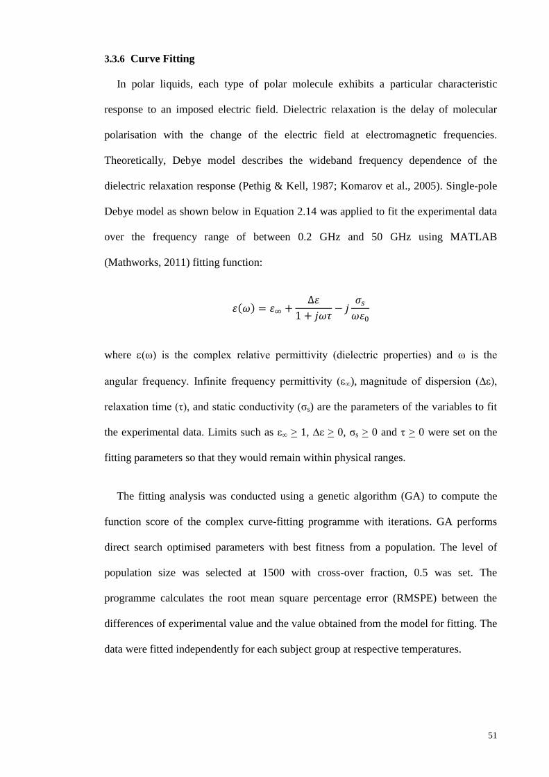
51

3.3.6 Curve Fitting

In polar liquids, each type of polar molecule exhibits a particular characteristic

response to an imposed electric field. Dielectric relaxation is the delay of molecular

polarisation with the change of the electric field at electromagnetic frequencies.

Theoretically, Debye model describes the wideband frequency dependence of the

dielectric relaxation response (Pethig & Kell, 1987; Komarov et al., 2005). Single-pole

Debye model as shown below in Equation 2.14 was applied to fit the experimental data

over the frequency range of between 0.2 GHz and 50 GHz using MATLAB

(Mathworks, 2011) fitting function:

( )

where (ω) is the complex relative permittivity (dielectric properties) and ω is the

angular frequency. Infinite frequency permittivity (ε∞), magnitude of dispersion (∆ε),

relaxation time (η), and static conductivity (ζs) are the parameters of the variables to fit

the experimental data. Limits such as ε∞ > 1, ∆ε > 0, ζs > 0 and η > 0 were set on the

fitting parameters so that they would remain within physical ranges.

The fitting analysis was conducted using a genetic algorithm (GA) to compute the

function score of the complex curve-fitting programme with iterations. GA performs

direct search optimised parameters with best fitness from a population. The level of

population size was selected at 1500 with cross-over fraction, 0.5 was set. The

programme calculates the root mean square percentage error (RMSPE) between the

differences of experimental value and the value obtained from the model for fitting. The

data were fitted independently for each subject group at respective temperatures.

52

3.4 Results

3.4.1 Urine Composition

As defined, glycosuria was found in DM subjects. The DM subjects were grouped

into three groups based on their urinary glycosuria levels: 0 g/L, >1 g/L and >5 g/L,

respectively. The characteristics of the subject groups are presented in Table 3.2.

Table 3.2: Characteristics of the DM subjects.

Group 1 2 3

Glycosuria level (g/L) 0 >1 >5

Total (N) 15 13 16

Age (years) 60 ± 9.7 59 ± 6.4 60 ± 10

HbA1c (%) 6.9 ± 1.0 7.6 ± 0.7 8.2 ± 1.3

Fasting Blood Glucose (mmol/L) 6.5 ± 1.4 7.6 ± 2.6 8.9 ± 2.4

3.4.2 Reproducibility and Accuracy

Reproducibility of the experiment was obtained by measuring the dielectric

properties of distilled water repeatedly 5 times at 25°C, 30°C and 37°C, respectively,

with independent calibration session as suggested by Gabriel and Peyman (2006) and

Zhadobov et al. (2012). According to Agilent Technologies (2012), the accuracy of the

measurement with coaxial slim probe is within ± 0.05 or ± 5% at temperature of 23 ±

3°C. To assess the accuracy of the technique, measurements for methanol and 0.1M salt

water were conducted. However, it is inappropriate for determining the experimental

accuracy at high temperature for methanol, which has different spectra of dielectric

properties with water, especially at the millimetre wave range (Zhadobov et al., 2012).

Thus, the measurement of methanol was conducted at 25°C. No significant differences

(p>0.05) were obtained among measured data at different calibration sessions at the

53

frequency range from 0.2 to 50 GHz. The reproducibility of measurements for urine was

the same with those obtained from reference liquids.

Figures 3.2 and 3.3 show the comparison of measured dielectric properties with

reference values of distilled water extracted from Ellison‘s database (Ellison et al.,

1996; Ellison, 2007). Overall, the measured data were closely matched to reference

data. Maximum deviations compared to reference data were about 4%.

Figure 3.2: Comparison between measured dielectric constant of distilled water

and reference data at respective temperatures of 25°C, 30°C and 37°C for

frequencies ranging from 0.2 to 50 GHz.

54

Figure 3.3: Comparison between measured loss factor of distilled water and

reference data at respective temperatures of 25°C, 30°C and 37°C for frequencies

ranging from 0.2 to 50 GHz.

Tables 3.3 and 3.4 show the comparison of Debye parameters for distilled water and

0.1M salt water with reference data, respectively. Overall, the measured data were close

to the reference data with deviation less than 1.5%.

55

Table 3.3: Comparison of Debye parameters of distilled water with reference

data at 25°C, 30°C and 37°C

Temperature

(°C)

∆ τ (ps) Study

25 73.38 8.20 (This study)

72.38 8.28 (Ellison, 2007)

- 7.36 (Johri & Roberts, 1990)

73.16 8.27 (Kaatze, 1989)

30 71.61 7.30 (This study)

70.83 7.35 (Ellison, 2007)


71.36 7.28 (Kaatze, 1989)

37 69.19 6.22 (This study)

68.71 6.29 (Ellison, 2007)


69.57 6.23 (Kaatze, 1989)

56

Table 3.4: Comparison of Debye parameters of 0.1M salt water with reference

data at 25°C, 30°C and 37°C

Temperature (°C) ∆ τ (ps) Study

25 71.67 8.08 (This study)

71.14 8.07 (Buchner et al., 1999)

30 68.50 7.19 (This study)

69.58 7.19 (Buchner et al., 1999)

37 67.91 5.98 (This study)

67.32 5.95 (Buchner et al., 1999)

Figure 3.4 shows the comparison between measured dielectric properties of methanol

with reference data presented in Gregory and Clarke (2001), Smith et al. (1998), and

Yomogida et al. (2012). Overall, the deviations were within 1~5 %.

Figure 3.4: The comparison between measured dielectric properties of methanol

with reference data at 25°C.

0

2

4

6

8

10

12

14

16

0

5

10

15

20

25

30

35

0 10 20 30 40 50

εr'' εr'

Frequency (GHz)

This study

Gregory and Clarke (2001)

Smith et al. (1998)

Yomogida et al. (2012)

εr''

εr'

57

3.4.3 Dielectric Properties of Glycosuria

3.4.3.1 Overview

The urinary dielectric properties were obtained from DM subjects with glycosuria

levels: 0 g/L, >1 g/L and >5 g/L at the respective temperatures of 25°C, 30°C and 37°C.

A closer look at the measured urinary dielectric properties of the subject groups is

presented in Figures 3.5 and 3.6 for wideband analysis of 0.2 GHz to 50 GHz at 25°C.

Meanwhile, the same trend was observed for 30°C and 37°C.

At low frequency ranges, less observable changes of urinary dielectric properties are

reported with glycosuria level. Subjects with glycosuria level >5 g/L showed the

increment of dielectric constant at frequency ranges between 0.2 GHz and 3 GHz, as

well as between 25 GHz and 40 GHz (Figure 3.5). The changes in urinary dielectric

properties with glycosuria level were prominent at higher frequencies. Dielectric

constant was increased, while loss factor was decreased with glycosuria level at

frequencies above 40 GHz and 15 GHz, respectively. Relaxation frequency was shifted

towards lower values with glycosuria level (Figure 3.6).

58

Figure 3.5: Urinary dielectric constant among subject groups at 25°C.

57

60

63

66

69

72

75

78

0 1 2 3 4 5 6 7 8 9 10 11 12

εr'

Frequency (GHz)

0 g/L

>1 g/L

>5 g/L

(a)

30

35

40

45

50

55

60

13 14 15 16 17 18 19 20 21 22 23 24

εr'

Frequency (GHz)

(b)

24

25

26

27

28

29

30

31

32

33

25 26 27 28 29 30 31 32

εr'

Frequency (GHz)

(c)

18

19

20

21

22

23

24

33 34 35 36 37 38 39 40

εr'

Frequency (GHz)

(d)

14

15

16

17

18

19

41 42 43 44 45 46 47 48 49 50

εr'

Frequency (GHz)

(e)

59

Figure 3.6: Urinary loss factor among subject groups at 25°C.

-5

0

5

10

15

20

25

30

35

0 1 2 3 4 5 6 7 8 9 10 11 12

εr''

Frequency (GHz)

0 g/L

>1 g/L

>5 g/L

(a)

34

35

36

37

13 14 15 16 17 18 19 20 21 22 23 24

εr''

Frequency (GHz)

(b)

32

33

34

35

36

25 26 27 28 29 30 31 32

εr''

Frequency (GHz)

(c)

28

29

30

31

32

33

33 34 35 36 37 38 39 40

εr''

Frequency (GHz)

(d)

24

25

26

27

28

29

41 42 43 44 45 46 47 48 49 50

εr''

Frequency (GHz)

(e)

60

3.4.3.2 Statistical analysis

Overall, the temperature of 25°C produced the strongest statistically significant

differences (p < 0.05) across subject groups compared to 30°C and 37°C. The highest

observed F number, F(2, 41) = 8.681; p < 0.01 was obtained at the frequency of 35.2

GHz between measured frequency range of 0.2 to 50 GHz. The statistically significant

difference was defined at critical F value, Fcrit ≥ 3.226. Table 3.5 shows the observed F

number and p-value of urinary dielectric properties across subject groups at different

microwave frequencies. There were stronger significant differences in the dielectric

constant across subject groups, compared to loss factor.

61

Table 3.5: F number and p-value of urinary dielectric properties across DM subject groups at different microwave frequencies

Frequency

(GHz)

25°C 30°C 37°C

εr’ εr’’ εr’ εr’’ εr’ εr’’

F

number

p-value F

number

p-value F

number

p-value F

number

p-value F

number

p-value F

number

p-value

0.2 1.045 0.359 0.597 0.554 1.267 0.290 0.536 0.588 1.635 0.205 0.633 0.535

0.4 1.308 0.279 0.788 0.460 1.153 0.324 1.754 0.183 1.664 0.199 0.824 0.444

0.6 1.577 0.216 0.954 0.392 1.104 0.339 2.274 0.113 1.796 0.176 1.170 0.318

0.8 1.708 0.191 0.789 0.460 0.836 0.439 1.593 0.213 1.969 0.150 1.717 0.189

1 2.051 0.139 0.877 0.422 0.793 0.458 1.977 0.149 2.038 0.140 1.576 0.216

3 0.201 0.818 0.654 0.524 1.429 0.249 3.012 0.058 0.749 0.478 2.056 0.138

5 3.898 0.026 0.422 0.658 0.539 0.586 1.145 0.326 1.555 0.221 1.397 0.256

10 4.886 0.011 0.056 0.945 2.388 0.102 0.468 0.629 1.045 0.359 1.303 0.280

30 7.648 <0.01 2.453 0.096 4.024 0.024 1.530 0.226 2.786 0.071 0.844 0.436

50 2.964 0.060 0.669 0.517 0.038 0.968 4.483 0.016 1.082 0.346 1.696 0.193

62

Table 3.6 shows the group-pairs that have significant differences in urinary dielectric

properties. Subjects with glycosuria level 0 g/L and >5 g/L showed the best pair group

significant differences of dielectric constant at 25°C, followed by subjects with

glycosuria level >1 g/L and >5 g/L. Meanwhile, subjects with glycosuria level 0 g/L and

>1 g/L showed no significant pair differences in the measured microwave frequency

range. The Pearson correlation test indicated that dielectric constant showed significant

positive correlation (r = 0.559; p < 0.01) with glycosuria level. Loss factor had

significant negative correlation (r = -0.491; p = 0.015) at >15 GHz.

Table 3.6: Significant differences in urinary dielectric properties of group-pairs

Frequency

(GHz)

25°C 30°C 37°C


0.2 - - - - - -

0.4 - - - - - -

0.6 - - - - - -

0.8 - - - - - -

1 - - - - - -

3 - - - - - -

5 1-3 - - - - -

10 1-3, 2-3 - - - - -

30 1-3, 2-3 - 1-3 - - -

50 - - - 1-3 - -

3.4.3.3 Comparison with Debye Model

Figure 3.7 shows the Cole-Cole diagram of experimental urinary dielectric properties

data fit to the Debye model for glycosuria subjects at 25°C. Overall, the experimental

data was fitted to the single-pole Debye model with deviations of about 0.5% ~ 2%.

63

Figure 3.7: Cole-Cole diagram of experimental urinary dielectric properties data

fit to the Debye model for glycosuria subjects at 25°C

Table 3.7 shows the Debye dielectric parameters of different glycosuria levels at

25°C, 30°C and 37°C, which were calculated using Equation 2.14. ∆ε and η increased,

and decreased with glycosuria level and temperature, respectively.

-5

0

5

10

15

20

25

30

35

40

15 25 35 45 55 65 75

εr''

εr'

Glycosuria

Debye fit

64

Table 3.7: Debye dielectric parameters of different glycosuria levels at 25°C, 30°C and 37°C

Glycosuria

Level (g/L)

25°C 30°C 37°C

ε∞ ∆ε τ

(ps)

σs

(S/m)

RMSPE

(%)

ε∞ ∆ε τ

(ps)

σs

(S/m)

RMSPE

(%)

ε∞ ∆ε τ

(ps)

σs

(S/m)

RMSPE

(%)

0 4.60 73.13 8.16 0.03 0.25 4.92 71.56 7.23 0.01 0.11 4.68 69.35 6.14 0.01 0.12

>1 4.77 74.30 8.69 0.02 0.13 4.85 71.73 7.55 0.01 0.11 4.57 69.46 6.22 0.02 0.18

>5 4.87 76.50 9.25 0.09 0.11 4.84 72.21 8.09 0.06 0.17 4.74 69.77 6.65 0 0.22

65

3.4.3.4 Classifications accuracy between glycosuria and non-glycosuria groups

In order to determine the accuracies of urinary dielectric properties to distinguish

between glycosuria and non-glycosuria groups, classifications were conducted based on

the threshold from the mean values of subject groups. Table 3.8 shows the classification

accuracies of urinary dielectric properties between glycosuria and non-glycosuria

groups at different temperatures. Overall, the deviations were about 7~17% and 3~15%

across different urinary dielectric properties and temperatures, respectively.

Table 3.8: Classification accuracies between non-glycosuria and glycosuria

groups at 25°C, 30 °C and 37°C

Dielectric

Properties

Classification Accuracy (%)

25°C 30°C 37°C

εr‘ 72.0 77.08 66.67

εr‘‘ 54.9 69.39 66.67

3.5 Discussion

3.5.1 Reproducibility and Accuracy

To report the urinary dielectric properties of glycosuria, additional reproducible and

accurate procedures were conducted at 30°C and 37°C in order to determine strong

temperature dependency of dielectric properties in high water content urine. Arai et al.

(1995) and Chen et al. (2004) reported that dielectric properties measured at

temperatures higher than room temperature produced lower accuracies due to technical

problems in thermal expansion and temperature gradient of the coaxial probe. To

overcome this issue, the coaxial slim probe was heated to 30°C and 37°C in a water bath

66

before measurements were taken at the respective temperatures. This increased the

reproducibility of measurements >90%.

In comparison between the measured data with reference data, the data of Johri and

Roberts (1990) shows the highest deviation with the measured data for water. They used

microwave resonant cavity perturbation technique to determine the dielectric response

of water. However, the technique is more suitable for measuring solids and low loss

materials as suggested by Venkatesh and Raghavan (2005), Komarov et al. (2005) and

Icier and Baysal (2004). Hence, measurement accuracy may be considered to differ

between two different techniques, cavity perturbation and open-ended coaxial probe

technique. Meanwhile, less comparison data was observed at high frequencies for

dielectric properties of methanol. The measurements of methanol are mostly available at

frequencies below 10 GHz, as the dielectric properties of methanol at milimeter waves

are considered too low to obtain reliable results from the technique in this study

(Kaatze, 2007). The appropriate method for measuring dielectric properties of biological

solutions with approximately 0.1M salt content has been validated by using open-ended

coaxial probe technique with accuracy > 95% (Table 3.4).

3.5.2 Effect of Temperature

In fact, the urine temperature may vary between the body and room temperature in

the process of measurement. Temperature variation is an important factor for dielectric

properties measurement. The spectra of dielectric properties of urine were observed to

be close to that of water since > 90% of urine is water content. Urinary dielectric

properties of subject groups were observed to change across temperatures from 25°C to

37°C. This could be due to the increase in temperature, which affects the stretching of

intramolecular hydrogen bonds and Brownian movement in solution that accounts for

the changes of dielectric properties (Robert et al., 1993; Komarov et al., 2005; Ellison,

67

2007). However, randomising the agitation of molecules at high temperature reduced

the significant effect of glucose. This result in the strongest statistically significant

differences (p < 0.05) across subject groups that were found at 25°C compared to 30°C

and 37°C. This study validated the reliability of dielectric measurement of glycosuria at

room temperature.

3.5.3 Effect of Glucose

Zhadobov et al. (2012) reported that glucose solutions below concentration 1% had

similar dielectric properties with distilled water. In this study, statistical analysis

showed that urinary dielectric properties had significant differences (p < 0.05) across

subject groups with different glycosuria levels at high frequencies. Correlation tests

validated the relationship of urinary dielectric properties with different glycosuria

levels.

According to Figure 3.5, dielectric constant showed an increasing trend at frequency

of 0.2 to 1 GHz, a finding which is in agreement with the study by Smulders et al.

(2013). The presence of salt content in urine (physiological solution) causes a decrease

of the dielectric constant compared to pure water at low frequencies (Smulders et al.,

2013). Different trends in glycosuria dielectric properties were observed compared to

glucose solution (Liao et al., 2001; Smulders et al., 2013). Lonappan et al. (2004) and

Lonappan et al. (2007a) reported that dielectric constant increased with glycosuria level

more than 1.5% at frequency of 2.4 to 3 GHz. The results are in agreement with

Lonappan et al. (2004) and Lonappan et al. (2007a). The dielectric constant was found

increased at physiological glycosuria level more than 5 g/L (> 0.5%) at frequency range

of 0.2 to 3 GHz, and 20 to 40 GHz, respectively. Significant correlation between urinary

dielectric properties and glycosuria levels were prominent at high frequencies (as shown

in Figure 3.5 and Figure 3.6). Maritim et al. (2003) found the presence of oxidative

68

stress in biological solution due to free radicals formed by glucose oxidation under

normal physiological condition that increases free charges. Studies reported higher free

radicals (8-iso prostaglandin F2α) in the urine of diabetic patients with glucose

variability compared to normal subjects (Monnier et al., 2006; Wentholt et al., 2008).

Increments in dielectric constant and relaxation time are due to the free radicals of

glucose bio-oxidation process that increases the density of dipoles (Abdalla et al.,

2010).

3.5.4 Comparison with Debye model

There is limited data available to compare the dielectric properties of urine. Peyman

and Gabriel (2012) compared the dielectric properties of porcine urine with Debye

model for frequency between 50 MHz and 20 GHz. Thus, comparison between

experimental data and Debye model is proposed. It is sufficient to model the

experimental dielectric data with single-pole Debye model using Equation 2.14, as a

main dispersion was observed at the measured frequency between 0.2 GHz and 50 GHz.

Overall, the experimental data were well fitted to the Debye model. The model appears

to be sufficient to estimate the dielectric evolution of urine. The deviations between

measured data and Debye fit data were mostly observed at low frequencies with about

2% (Figure 3.7). This may be due to the instability of the high frequency dielectric

system to measure low frequencies below 1 GHz. However, the variations were within

the acceptable range of standard error of ± 5%.

According to Table 3.7, ε∞ was close to 5 across all the subject groups and

temperatures as the major component of urine is water molecules. This indicates that the

water content of urine was not affected in glycosuria. Peyman and Gabriel (2010) and

(2012) reported that the variation of up to 25% for the value of ε∞ has very little impact

on the other fitted parameters. ∆ε and η were found to increase with glycosuria level, but

69

decrease with temperature. The strength of changes across subject groups was observed

to decrease with temperature from 25°C to 37°C. Dielectric properties of glycosuria

were more prominent at room temperature (25°C) rather than at body temperature

(37°C). Static conductivity, ζs was negligible across subject groups and temperatures.

Conductivity of urine was relatively small in a constant field as human physiological

solution is quoted to have only about 0.9% of salt content (Nörtemann et al., 1997;

Smulders et al., 2013). The temperature and glycosuria level affect the overall urinary

dielectric dispersion and relaxation.

3.5.5 Classification across Glycosuria and Non-glycosuria Groups

According to Table 3.8, temperature effects were observed in the classification

accuracies of overall urinary dielectric properties. Among the three measured

temperatures, 30°C showed the highest classification accuracies. Meanwhile, dielectric

constant was found to produce higher classification accuracies than loss factor at 25°C

and 30°C. However, bias may occur in this classification method due to its dependence

on the threshold (mean) differences across subject groups. This remains a challenge in

carrying out cross-comparison with other methods.

3.6 Summary

In this chapter, the urinary dielectric properties of subjects with Type 2 DM at

microwave frequency between 0.2 GHz and 50 GHz were investigated. Glycosuria

variability among subjects groups was described. The effect of temperature was

determined in the changes of urinary dielectric properties with respective glycosuria

level. Statistical correlation between urinary dielectric properties and glycosuria level

was identified. Additional classifications were conducted to distinguish between

glycosuria and non-glycosuria groups.

70

Room temperature (25°C) produced the strongest statistically significant difference

in urinary dielectric properties for the change of glycosuria level. The results obtained

showed that dielectric constant increased with glycosuria level more than 5 g/L (0.5%)

at low frequencies. Dielectric constant correlated positively with glycosuria level at

frequencies above 40 GHz. Loss factor correlated negatively with glycosuria level at

frequencies above 15 GHz. The experimental data were fitted to the single-pole Debye

model. This found that the experimental data were closely matched with the Debye

model. The urinary dielectric dispersion and relaxation time increased with glycosuria

level, while decreased with temperature. In classifications, dielectric constant produced

higher accuracies than loss factor. Different temperatures were observed affecting the

overall classification accuracies. However, this remains a challenge in cross-comparison

with other classification methods.

71


PROPERTIES OF PROTEINURIA FOR CHRONIC KIDNEY DISEASE

4.1 Introduction

Urinary protein is defined as an early sign of CKD. Persistent proteinuria followed by

progressive decline of renal function (increments in serum creatinine level) are

presentations of CKD and this eventually leads to end stage renal disease (Epstein et al.,

1998). The presence of proteinuria has been identified in patients with increased risk of

CKD progression (Iseki et al., 2004; Ishani et al., 2006). The changes in dielectric

properties of solutions with respect to animal protein concentration indicate the

potential application of dielectric properties measurement in proteinuria. So far, no

studies have been conducted to look into the urinary dielectric properties of proteinuria.

No data has been reported for changes in the urinary dielectric properties of proteinuria

with temperature.

In this chapter, the urinary dielectric properties of normal subjects and subjects with

CKD at room temperature (25°C), 30°C and body temperature (37°C), respectively, at

microwave frequency between 0.2 GHz and 50 GHz are investigated. This chapter

determines the significant differences in urinary dielectric properties among subjects

with different proteinuria levels. The correlations between urinary dielectric properties

and proteinuria level are investigated. The measured data are fitted to Debye model for

comparison.


4.2.1 Overview of Kidney Disease

The kidneys are organs of blood purification. They remove metabolic waste such as

excessive water, salt and toxins in the form of urine from the human body and perform

homeostatic functions. Patients with either DM, hypertension, urinary tract

72

abnormalities, systemic autoimmune disorder, excessive use of known toxins and

systems suggestive of systemic illness develop higher risk of getting CKD (American

Diabetes Association, 1998).

Kidney disease is classified into acute and CKD. Acute kidney disease such as

polycystic kidney disease occurs suddenly due to many cysts or cavities being formed in

the kidneys while pyelonephritis is caused by kidney infection. Meanwhile, CKD occurs

when there is a long period of kidney deficiency. Patients seldom have symptoms at the

early stage of CKD.

Overall, CKD is classified in terms of diabetic kidney disease (DKD) and non-

diabetic kidney disease (non-DKD). Type 2 DM is the primary cause of kidney failure

among the population (Feisul & Azmi, 2012; American Diabetes Association, 2014).

High level of blood glucose causes kidneys to produce extra force to maintain the

necessary filtering processes. The extra forces required may cause the capillaries in the

kidneys to leak, allowing loss of glucose and protein in the urine. Eventually, the

kidneys lose their ability to function and waste products will accumulate in the blood

(American Diabetes Association, 1998; Kanwar et al., 2008).

4.2.1.1 Chronic kidney disease diagnosis and monitoring

Current clinical determination uses estimated glomerular filtration rate (eGFR) to

diagnose the overall kidney function and stages of CKD. However, eGFR that uses

concentration of serum creatinine may be affected by factors such as gender, age,

ethnicity, medication, muscle mass and protein intake (Lascano & Poggio, 2010).

Furthermore, CKD seldom has clinical symptoms in the early stage.

Urinary protein is defined as an early sign of CKD. Urinary protein excretion is

important to identify, characterise and monitor the progression of CKD. Zürbig et al.

73

(2009) reported initial pathophysiological changes in kidneys, resulting in significant

changes of urinary proteins, which are potential biomarkers at the early stage of CKD.

Protein increases in urine with respect to the stages of CKD (Ghiggeri et al., 1985).

Monitoring of urinary protein is required as standard care in diagnosis and

prognostication of patients with risk factors of CKD.


4.3.1 Subject Recruitment

A total of 43 subjects with CKD (disease duration of >3 years) were recruited from

the outpatient clinics at the University of Malaya Medical Centre (UMMC). Exclusion

criteria involved DKD subjects and bladder-related diseases such as presence of

glycosuria or haematuria. A total of 40 subjects were recruited as normal, which

involved healthy subjects who were recruited at the University of Malaya, Malaysia.

Normal subjects without history of kidney or bladder-related diseases were recruited.

Medical ethics approval was obtained from the Institutional Ethics Review Committee,

UMMC. All subjects provided written informed consent to participate in this study.

4.3.2 Urine Collection and Storage

Sixty ml of random spot mid-stream urine samples were collected from each subject.

For each collected urine sample, 20 ml was used to measure urinary clinical chemical

variables and microscopy using routine methods at the Division of Laboratory

Medicine, UMMC.

Urine samples were collected in sterile urine containers. Fresh urine samples were

stored at a temperature of 4°C within 4 hours before the measurement of dielectric

properties was conducted. No preservatives were added upon urine collection.

74

4.3.3 Urine Measurements

The measurement setup is as described in the previous chapter (Chapter 3). Before

measurements were conducted, urine samples were heated to room temperature (25°C)

using a WNB 7 water bath (Memmert, Duesseldorf, Germany) with a precision of ±

0.1°C and the samples were gently stirred. Random and systemic errors were taken into

account to reduce uncertainties as reported by Gabriel and Peyman (2006). Experiments

were repeated by heating the urine samples to 30°C and 37°C, respectively. For each

experiment, three measurement readings were recorded for each urine sample

throughout the frequency range of 0.2 to 50 GHz.

4.3.4 Data Analysis

Dielectric properties, in terms of dielectric constant (r‘) and loss factor (r

‘‘), were

obtained from the measurements. A total of 250 frequency points were measured with

an interval of 200 MHz at the microwave frequency range of 0.2 to 50 GHz. The

Independent Samples T test of SPSS Statistic 21.0 (IBM Corp, 2012) was used to

determine the statistically significant differences between urinary dielectric properties

and urine composition of normal and CKD subjects. The statistical one-way analysis of

variance (ANOVA) test was conducted to determine the respective effects of proteinuria

and temperature in the urinary dielectric properties at different microwave frequencies.

Pearson correlation test was conducted to determine correlation between proteinuria

levels and urinary dielectric properties. The level selected for statistical significance (p-

value) was set at probability value <0.05.

4.3.5 Curve Fitting

Single-pole Debye model as shown below in Equation 2.14, was applied to fit the

experimental data over the frequency range of between 0.2 GHz and 50 GHz using

MATLAB (Mathworks, 2011) fitting function:

75

( )

where (ω) is the complex relative permittivity (dielectric properties) and ω is the

angular frequency. Infinite frequency permittivity (ε∞), magnitude of dispersion (∆ε),

relaxation time (η) and static conductivity (ζs) are the parameters of the variables to fit

the experimental data. Limits such as ε∞ > 1, ∆ε > 0, ζs > 0 and η > 0 were set on the

fitting parameters so that they would remain within physical ranges.

The fitting analysis was conducted using a genetic algorithm (GA) to compute the

function score of the complex curve-fitting programme with iterations. GA performs

direct search optimised parameters with best fitness from a population. The level of

population size was selected at 1500 with cross-over fraction, 0.5 was set. The

programme calculates the root mean square percentage error (RMSPE) between the

differences of experimental value and the value obtained from the model for fitting. The

data were fitted independently for each subject group at respective temperatures.

4.4 Results

4.4.1 Urine Composition

As defined, proteinuria was found in CKD subjects. Overall, lower levels of mean

creatinine, urea and salt ions were found in the urine of CKD subjects compared to

normal subjects (Table 4.1). This could be explained by the fact that CKD patients

suffer from kidney malfunction, which affects the body‘s efficiency in removing waste

and also causes leakage of protein into the urine. CKD subjects were grouped based on

their urinalysis proteinuria levels: >0.25 g/L, >0.75 g/L, >1.5 g/L and >5 g/L,

respectively. The characteristics of the subject groups are presented in Table 4.2.

76

Table 4.1: Chemical variables of normal and CKD subjects

Chemical Variables Normal CKD

Creatinine (μmol/L) 8846 ± 2677 6032 ± 1951

Urea (mmol/L) 183 ± 25 118 ± 46

Cl- (mmol/L) 103 ± 66 85 ± 33

Na+(mmol/L) 90 ± 59 83 ± 31

K+ (mmol/L) 32 ± 26 25 ± 13

Table 4.2: Characteristics of the CKD subjects

Characteristics Proteinuria level (g/L)

>0.25 >0.75 >1.5 >5

Total (N) 16 10 10 7

Age (years) 70 ± 11 67 ± 6 67 ± 10 54 ± 19

Serum creatinine (µmol/L) 184 ± 72 209 ± 74 219 ± 83 248 ± 68

4.4.2 Dielectric Properties of Proteinuria

4.4.2.1 Overview

The measurements of urinary dielectric properties were obtained from normal and

CKD subjects, and are presented in Figures 4.1 and 4.2. Urinary dielectric properties

showed different trends with temperature over the frequencies for normal and CKD

subjects. A ‗cross-over‘ frequency point was observed at about 7 GHz for the dielectric

constant and 27 GHz for the loss factor. The urinary dielectric properties were constant

over the changes of temperature and subject groups at the respective ‗cross-over‘

frequency point. Below this frequency point, the urinary dielectric properties decreased

with temperature. Urinary dielectric properties of CKD subjects were found to be higher

77

than those of normal subjects. Meanwhile, urinary dielectric properties increased with

temperature above the ‗cross-over‘ point. The CKD subjects had lower urinary

dielectric properties than those of the normal subjects above the frequency point.

Generally, the urinary dielectric properties showed more differences between the normal

and CKD subjects as the temperature increased from 25°C to 37°C.

Figure 4.1: Urinary dielectric constant of normal and CKD subjects at respective

temperatures of 25°C, 30°C and 37°C for frequencies ranging from 0.2 to 50 GHz.

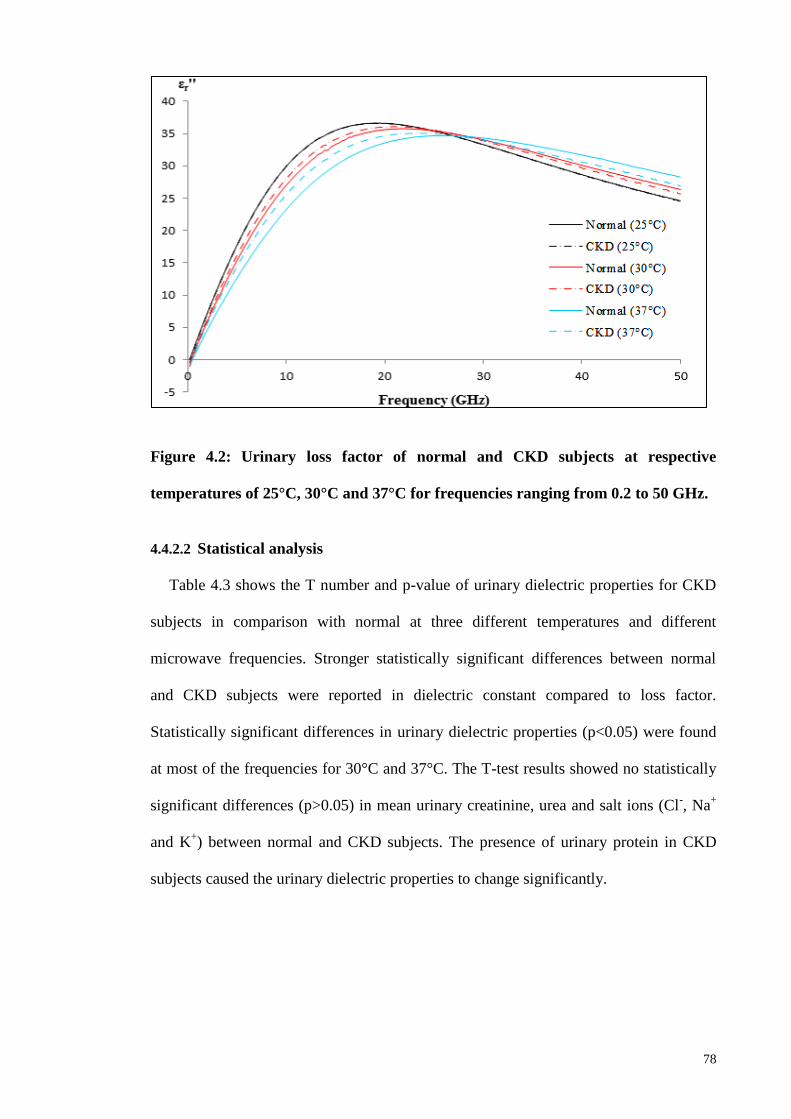
78

Figure 4.2: Urinary loss factor of normal and CKD subjects at respective

temperatures of 25°C, 30°C and 37°C for frequencies ranging from 0.2 to 50 GHz.

4.4.2.2 Statistical analysis

Table 4.3 shows the T number and p-value of urinary dielectric properties for CKD

subjects in comparison with normal at three different temperatures and different

microwave frequencies. Stronger statistically significant differences between normal

and CKD subjects were reported in dielectric constant compared to loss factor.

Statistically significant differences in urinary dielectric properties (p<0.05) were found

at most of the frequencies for 30°C and 37°C. The T-test results showed no statistically

significant differences (p>0.05) in mean urinary creatinine, urea and salt ions (Cl-, Na

+

and K+) between normal and CKD subjects. The presence of urinary protein in CKD

subjects caused the urinary dielectric properties to change significantly.

79

Table 4.3: T number and p-value of urinary dielectric properties for CKD subjects in comparison with normal at three different

temperatures and different microwave frequencies

Frequency

(GHz)

25°C 30°C 37°C


T

number

p-

value

T

number

p-

value

T

number

p-

value

T

number

p-

value

T

number

p-

value

T

number

p-

value

0.2 -1.465 0.147 -1.592 0.115 1.201 0.233 -1.428 0.157 3.880 <0.01 -0.663 0.509

0.4 -0.330 0.742 -2.564 0.012 2.688 <0.01 -1.468 0.146 4.497 <0.01 -0.013 0.989

0.6 0.562 0.576 -2.182 0.032 3.861 <0.01 -0.596 0.553 4.939 <0.01 0.972 0.334

0.8 1.237 0.220 -1.192 0.059 4.125 <0.01 -0.068 0.946 4.911 <0.01 2.078 0.041

1 1.592 0.115 -1.428 0.157 4.381 <0.01 0.847 0.400 4.903 <0.01 2.954 <0.01

3 -0.848 0.399 0.127 0.899 4.108 <0.01 3.760 <0.01 4.187 <0.01 4.552 <0.01

5 0.749 0.456 -0.613 0.542 2.626 0.01 4.476 <0.01 4.443 <0.01 4.568 <0.01

10 1.276 0.206 -0.174 0.862 -4.868 <0.01 4.474 <0.01 -4.185 <0.01 4.416 <0.01

30 -0.558 0.578 -0.880 0.381 -4.728 <0.01 -2.065 0.042 -4.282 <0.01 -4.653 <0.01

50 -0.582 0.562 -1.546 0.126 -4.575 <0.01 -3.724 <0.01 -4.213 <0.01 -4.191 <0.01

80

Table 4.4 indicates the F number and p-value of urinary dielectric properties across

proteinuria levels at different microwave frequencies. Overall, the temperature of 37°C

produced the strongest statistically significant differences (p<0.05) across proteinuria

subject groups compared to 25°C and 30°C. The highest observed F number, F(3, 39) =

9.598; p < 0.01 was obtained at 30 GHz of measured frequency range from 0.2 to 50

GHz. The statistically significant differences were defined at critical F value, Fcrit ≥

2.845. Dielectric constant had stronger significant differences than loss factor across

proteinuria subject groups.

81

Table 4.4: F number and p-value of urinary dielectric properties across proteinuria levels at different microwave frequencies

Frequency

(GHz)

25°C 30°C 37°C


F

number

p-

value

F

number

p-

value

F

number

p-

value

F

number

p-

value

F

number

p-

value

F

number

p-

value

0.2 0.288 0.834 2.533 0.115 1.107 0.107

1.135 0.346

5.997 <0.01

1.108 0.359

0.4 1.041 0.385 6.574 0.012

4.267 <0.01

1.575 0.189

8.242 <0.01

1.672 0.165

0.6 1.077 0.370

4.760 0.032

6.600 <0.01

1.527 0.202 9.293 <0.01

2.450 0.053

0.8 1.084 0.367

3.657 0.059 7.065 <0.01

1.815 0.134

8.994 <0.01

3.490 0.11

1 0.314 0.815

2.039 0.157 7.730 <0.01

1.997 0.103

8.819 <0.01

4.893 <0.01

3 1.046 0.383 0.016 0.899 6.425 <0.01

7.993 <0.01

6.421 <0.01 8.844 <0.01

5 0.773 0.516 0.376 0.542 3.804 <0.01

8.521 <0.01

8.014 <0.01 8.349 <0.01

10 2.587 0.067 0.030 0.862 7.651 <0.01

7.806 <0.01

7.272 <0.01 7.728 <0.01

30 0.300 0.585 1.956 0.109 7.740 <0.01

3.779 <0.01

7.242 <0.01 9.598 <0.01

50 1.391 0.245 1.436 0.230 6.466 <0.01

6.013 <0.01

6.681 <0.01 7.566 <0.01

82

Figure 4.3 shows observable changes in urinary dielectric properties with proteinuria

level at 37°C. Pearson correlation test showed positive correlation between proteinuria

level and urinary dielectric properties [rdielectric constant (43) = 0.568, p < 0.01; rloss factor (43)

= 0.564; p < 0.01] below the ―cross-over‖ frequency point, while negative correlation

[rdielectric constant (43) = - 0.535, p < 0.01; rloss factor (43) = - 0.505; p < 0.01] was found

above the ―cross-over‖ frequency point at 37°C. Less significant correlation was found

at 25°C.

Figure 4.3: Urinary dielectric properties of different proteinuria levels at 37°C

4.4.2.3 Comparison with Debye model

Figure 4.4 shows the Cole-Cole diagram of experimental urinary dielectric properties

data fit to the Debye model for normal and CKD subjects at 37°C. The experimental

data was fitted to the single-pole Debye model with deviations of about 0.5%~3%.

-5

0

5

10

15

20

25

30

35

40

0

10

20

30

40

50

60

70

80

0 5 10 15 20 25 30 35 40 45 50

εr'' εr'

Frequency (GHz)

>0.25 g/L >0.75 g/L

>1.5 g/L >5 g/L

83

Figure 4.4: Cole-Cole diagram of experimental urinary dielectric properties data

fit to the Debye model for normal and CKD subjects at 37°C

Table 4.5 shows Debye parameters of different proteinuria levels at 25°C, 30°C and

37°C, respectively. ∆ε and η were found to increase with proteinuria level, while

decreasing with temperature.

0

5

10

15

20

25

30

35

40

15 25 35 45 55 65 75

εr''

εr'

Normal Debye fit

CKD Debye fit

84

Table 4.5: Debye dielectric parameters of different proteinuria levels at 25°C, 30°C and 37°C

Proteinuria

Level (g/L)

25°C 30°C 37°C

ε∞ ∆ε τ

(ps)

σs

(S/m)

RMSPE

(%)

ε∞ ∆ε τ

(ps)

σs

(S/m)

RMSPE

(%)

ε∞ ∆ε τ

(ps)

σs

(S/m)

RMSPE

(%)

0 (Normal) 4.99 72.75 8.20 0.02 0.22 4.98 71.31 7.15 0.02 0.19 4.94 69.30 6.11 0.06 0.28

>0.25 5.06 72.83 8.23 0.01 0.17 4.86 71.87 7.26 0.01 0.22 4.89 69.83 6.35 0.02 0.18

>0.75 5.03 73.17 8.26 0.01 0.48 4.96 72.26 7.43 0.02 0.47 4.92 70.56 6.73 0.06 0.45

>1.5 4.97 73.19 8.27 0.05 0.18 5.02 72.59 7.64 0.07 0.21 5.08 71.55 7.11 0.08 0.26

>5 5.02 73.22 8.30 0.11 0.20 4.93 73.01 7.96 0.12 0.42 5.02 72.91 7.63 0.14 0.39

85

1.1.1.4 Accuracy of classifications between normal and CKD subjects

In order to determine the accuracy of urinary dielectric properties to distinguish

between normal and CKD subjects, additional classifications were conducted based on

the threshold from the mean values of subject groups. Table 4.6 shows the classification

accuracies of urinary dielectric properties between normal and CKD subjects at

different temperatures.

Table 4.6: Classification accuracies between normal and CKD subjects at 25°C,

30 °C and 37°C

Dielectric

Properties

Classification Accuracy (%)

25°C 30°C 37°C

εr‘ 59.72 68.67 79.52

εr‘‘ 72.29 69.88 51.81

4.5 Discussion

4.5.1 Effect of Temperature

Significant differences in urinary dielectric properties between normal and CKD

subjects were observed to be affected by the measured temperatures. The dielectric

properties of solutions change with temperature, due to the stretching of intramolecular

hydrogen bonds between water molecules (Ellison, 2007). As the temperature increased,

the relaxation time (η = 1/2пfc) of urine decreased. The increment in molecular

movement and ion mobility decreased the viscosity of the solution when the

temperature increased. Relaxation frequency is inversely proportional to the viscosity of

the solution (Komarov et al., 2005).

86

The temperature of 37°C produced the strongest statistically significant differences

(p<0.05) in urinary dielectric properties between normal and CKD subjects (Table 4.3)

and across proteinuria subject groups (Table 4.4). The effect of urinary protein is more

prominent at higher temperatures compared to 25°C and 30°C. This could be explained

by the urinary protein results in linear conduction rather than the oscillation motion of

the electrical field when the temperature changes (Pethig & Kell, 1987; Abdalla et al.,

2010).

4.5.2 Effect of Protein

Statistical analyses showed that the presence of proteinuria in CKD subjects caused

the urinary dielectric properties to change significantly (p<0.05), especially at 30°C and

37°C. Relaxation frequency was found to shift to lower frequencies when proteinuria

levels increased (Figure 4.3). As the proteinuria level increases, it decreases the bulk

water concentration that causes slower relaxation time scale to replace the faster

relaxation time scale of bulk water (Nandi & Bagchi, 1998). Previous studies have

reported the changes in dielectric properties of extracted protein solutions in radio

(Ferry & Oncley, 1938; Oncley, 1938) and microwave frequencies (Zhadobov et al.,

2012). Proteinuria was observed to have similar effects as protein solution in the

changes of dielectric properties. Although protein may not be as massive as other

components in complex biological solutions, however, additional substances

significantly alter the electrical properties of the solution (Abdalla et al., 2010).

Desouky (2009) discovered that glucose in blood (DM) drastically changed the

dielectric properties of blood. Urine is a complex biological solution similar to blood.

When water is protein-bound, it affects the linear conduction in urine, and this causes

drift scatter motion along the electrical field side that changes the overall dielectric

properties (Pethig & Kell, 1987; Abdalla et al., 2010).

87

4.5.3 Comparison with Debye Model

A main dielectric dispersion was observed at the measured frequency between 0.2

GHz and 50 GHz. Hence, it is sufficient to model experimental data with single-pole

Debye model using Equation 2.14. Overall, the experimental data were well fitted to the

Debye model for normal and CKD subjects. The deviations between experimental and

theoretical data were mostly observed at low frequencies, at about 2%~3%. This may be

due to the instability of the dielectric system to measure low frequencies at below 1

GHz. However, the variations were within the acceptable range of standard error of ±

5%.

According to Figure 4.4, observable different static permittivity, εs between normal

and CKD subjects were obtained. ε∞ was assumed to reach a constant for normal and

CKD subjects, although it was not within our measured frequency range. The

temperature and proteinuria level affect the overall urinary dielectric dispersion and

relaxation (Table 4.5). ε∞ was obtained as approximately constant (ε∞ ≈ 5) across all the

proteinuria levels and temperatures. This indicates that the water content of urine

remained unchanged for different proteinuria levels. Peyman and Gabriel (2010, 2012)

mentioned that the variation of about 25% on the value of ε∞ has very little effect on the

other fitted parameters. The relaxation amplitude, ∆ε and relaxation time, η increased

with proteinuria level, but decreased with temperature. The changes were observed to be

stronger at a higher temperature (37°C). The urinary dielectric properties of proteinuria

were certainly more prominent at body temperature (37°C) rather than at room

temperature (25°C). Static conductivity, ζs was negligible (ζs ≈ 0) at low proteinuria

levels. Conductivity of urine was relatively small in a constant field as biological

solution is quoted to have only about 0.9% (0.1 M) of salt content (Nörtemann et al.,

1997; Smulders et al., 2013). However, slight increase of ζs was observed with

temperature and proteinuria level reaching 1.5 g/L and 5 g/L, respectively. This remains

88

a challenge for conductivity determination from measured spectra at limiting low

frequencies.

4.5.4 Classifications between Normal and CKD Subjects

According to Table 4.6, different temperatures were observed affecting the overall

urinary dielectric properties classification accuracies. The classification accuracy of

dielectric constant was observed to increase, while the loss factor decreased with

temperature. The deviations were about 1~27% across different urinary dielectric

properties. However, bias may occur in this classification method due to its dependence

on the threshold (mean) differences across subject groups. Cross-comparison with other

classification methods is required.

4.6 Summary

In this chapter, the urinary dielectric properties of normal subjects and those with

CKD at microwave frequency between 0.2 GHz and 50 GHz were investigated. The

urine composition variations of normal and CKD subjects groups were described.

Proteinuria was found in CKD subjects. Overall, lower levels of urinary creatinine, urea

and salt ions were reported in CKD subjects compared to normal subjects. The effect of

temperature was determined in the changes of urinary dielectric properties with

proteinuria level. Statistical correlation between urinary dielectric properties with

proteinuria level was identified. Additional classifications were conducted to distinguish

between normal and CKD subjects.

The strongest statistically significant differences across proteinuria levels were

observed at body temperature (37°C). Urinary dielectric properties correlated positively

and negatively with proteinuria level below and above its ―cross-over‖ frequency points,

respectively. The experimental data were fitted to the single-pole Debye model. This

found that the experimental data closely matched the Debye model. The urinary

89

dielectric dispersion and relaxation time increased with proteinuria level, but decreased

with temperature. The classification accuracy of dielectric constant increased, while loss

factor decreased with temperature. However, cross-comparison with other classification

methods remains a challenge.

90

CHAPTER 5: CLASSIFICATION OF URINARY DIELECTRIC PROPERTIES

FOR TYPE 2 DIABETES MELLITUS AND CHRONIC KIDNEY DISEASE

5.1 Introduction

From the previous chapter, it can be seen that the measurement of dielectric

properties offers the potential to determine the variability of glycosuria and proteinuria

in a simple and non-destructive manner. The accuracy of the determination should be

investigated in order to show the potential of urinary dielectric properties to differentiate

among DM, CKD and normal subjects. Data classification has been used as the most

intensively studied method in statistical and decision science. Applications of SVM

classification for kidney disease (Haubitz et al., 2005; Kistler et al., 2009; Alkhalaf et

al., 2010; Gronwald et al., 2011), DM (Ban et al., 2010; Roshan et al., 2011) and

cancers (Kerhet et al., 2006; Laufer & Rubinsky, 2009; Shini et al., 2011; Gonzalez et

al., 2013; Grewal & Golnaraghi, 2014) have validated the capability of SVM as a

classifier. Ideally, a desirable diagnostic tool for DM and CKD would be one that is

non-invasive and highly accurate by measuring urinary dielectric properties.

In this chapter, the urinary dielectric properties of normal subjects, subjects with

Type 2 DM and subjects with CKD at room temperature (25°C), 30°C and body

temperature (37°C) between microwave frequencies ranging from 1 GHz to 50 GHz are

classified. SVM-based classification was applied and the effect of temperature in

classification accuracy is determined.


5.2.1 Inner-Product Kernel

For nonlinear classification, inner-product Kernel function is used in SVM. It

converts nonlinear input data into high dimensional linear feature space. Theoretically, x

is a vector from the input space with assumed dimensional m0 and 1

{ ( )} im

jx

is a set of

91

non-linear transformation from input space to feature space, m1. Hyperplane for the

decision surface of nonlinear transformation is as follows:

∑ ( )

5.1

where 1

1{ }

m

j jw

is a set of linear weights that connects feature space to output space

and b is the bias. ( )j

x of the inputs to the weight, wj through the feature space. The

vector is defined as follows:

( ) , ( ) ( ) ( )- 5.2

where ( ) for all x. The decision surface may be defined in compact form

since ( ) represents the ―image‖ in feature space due to x.

( ) 5.3

where ∑ ( ) and ( ) is the feature vector representing input pattern

xi in ith examples. Hence,

∑ ( ) ( )

5.4

The inner-product Kernel denoted by K(x,xi ) and defined by

92

( ) ( ) ( ) ∑ ( ) ( )

5.5

Inner-product Kernel, K(x,xi ) is used to construct optimal hyperplane in the feature

space, considering feature space in the explicit form. Figure 5.1 shows the architecture

of SVM that constructs a decision classification for non-linear input space.

Figure 5.1: Architecture of SVM for non-linear classification.

5.2.2 Model Selection

Inner-product Kernel must satisfy the Mercer‘s theorem (Haykin & Network, 2004).

Classifier accuracy on the hyperparameters is dependent on the decision boundary of the

SVM. A set of parameters called hyperparameters that includes the soft-margin, C and

other parameters of the kernel functions dependence (Table 2.5) for SVM are needed to

be tuned. Soft-margin constant, C is assigned to margin errors. It represents the two

points closest to the hyperplane that affect the orientation. When C value is decreased, it

provides a larger margin for the data and allows ignoring points that are close to the

boundary. For Kernel parameters, the degree of polynomial kernel, p and the width

parameter, of the radial basis function (RBF) kernel control the flexibility of the

classifier. The increase of p value yields greater curvature of the decision boundary.

93

When value is less, the boundary is nearly linear. The flexibility of the boundary

increases with value. However, the large value of causes overfitting of data where

the discriminant function is constant over the outer side in close proximity to the region.

Ben-Hur and Weston (2010) suggested that RBF and polynomial kernel may cause

overfitting in high-dimensional database with a small number of samples. RBF kernel

usually performs better in terms of accuracy and time convergence compared to

polynomial kernel.


5.3.1 Data Source

The database was obtained from the urinary dielectric properties of Type 2 DM,

CKD and normal subjects at microwave frequency ranging from 1 GHz to 50 GHz.

Subjects involved a total of 102 subjects with DM, 232 subjects with CKD and 97

healthy subjects. Subjects with CKD were further classified into diabetic kidney disease

(DKD) with n=102 and non-DKD (n=130). The description of the database and clinical

characteristics of the subjects are shown in Table 5.1 and Table 5.2, respectively.

94

Table 5.1: Database of DM, CKD and normal subjects

Subject DM DKD Non-DKD Normal

Male 54 68 79 51

Female 48 34 51 46

Total 102 102 130 97

Table 5.2: Clinical characteristics of DM, DKD, non-DKD and normal subjects.

Subject DM DKD Non-DKD Normal

Age (years) 61 ± 9 65 ± 10 64 ± 12 27 ± 8

Systolic BP (mmHg) 146 ± 26 147 ± 20 137 ± 19 115 ± 10

Diastolic BP (mmHg) 77 ± 17 74 ± 13 72 ± 14 72 ± 7

Serum creatinine (μmol/L) <115 248 ± 149 218 ± 107 <115

eGFR (ml/min per 1.73m2) >90 21 ± 12 27 ± 16 >90

Proteinuria level (g/L) - 2.71 ± 1.11 2.15 ± 1.30 -

Glycosuria level (g/L) 4.62 ± 2.18 3.08 ± 2.70 - -

95

5.3.2 Classification Model

SVM-based classification of urinary dielectric properties was performed using

LIBSVM tool (Chang & Lin, 2011) in MATLAB software (Mathworks, 2011). A total

of 50 variables (microwave frequency from 1 GHz to 50 GHz) of urinary dielectric

properties were used as the inputs to the classification model. Classification was

accomplished based on 3-fold cross validation method. Two-thirds of the database was

used as training set and the remaining one-third was used for validation. The

classification was repeated three times based on different training and validation sets

from the same database. The prediction accuracies were obtained from the average of

three test sets. RBF kernel, ( ) ( ‖ ‖ ) was applied with the

parameter, [0.1, 10] and was tested in the system to determine the optimal

classification accuracy. Classification models were generated based on the respective

urinary dielectric constant and loss factor at 25°C, 30°C and 37°C, respectively. The

classifiers were applied to the database to predict the disease of the subjects based on

different urinary dielectric properties.

5.4 Results

5.4.1 Overview

The cross-comparisons of mean urinary dielectric properties for different subject

groups are presented in Figure 5.2 at respective temperatures of 25°C, 30°C and 37°C.

Differences in urinary dielectric properties were observed in comparison between DKD

and normal, non-DKD and normal, and DKD and non-DKD subject groups,

respectively. DKD subjects had lower and higher urinary dielectric properties than non-

DKD subjects below and above its ‗cross-over‘ frequency point, respectively.

96

(a)

(b)

97

(c)

Figure 5.2: Comparison of mean urinary dielectric properties among DKD, Non-

DKD and normal subject groups.

5.4.2 Two-group Classification: DM vs Normal, DKD vs Normal and Non-DKD vs

Normal

The classifications were performed using urinary dielectric properties database with

50 variables and 431 records for dielectric constant and loss factor, respectively. RBF

kernel with = 0.5 was found to show optimal performance in classifications.

Classification results of urinary dielectric properties between DM vs normal, DKD vs

normal and non-DKD vs normal group at 25°C, 30°C and 37°C, respectively are

summarised in Table 5.3 to Table 5.5.

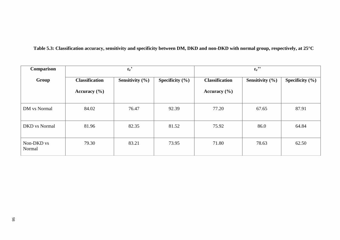
98

Table 5.3: Classification accuracy, sensitivity and specificity between DM, DKD and non-DKD with normal group, respectively, at 25°C

Comparison

Group

εr’ εr’’

Classification

Accuracy (%)

Sensitivity (%) Specificity (%) Classification

Accuracy (%)

Sensitivity (%) Specificity (%)

DM vs Normal 84.02 76.47 92.39 77.20 67.65 87.91

DKD vs Normal 81.96 82.35 81.52 75.92 86.0 64.84

Non-DKD vs

Normal

79.30 83.21 73.95 71.80 78.63 62.50

99


Comparison

Groups

εr’ εr’’

Classification

Accuracy (%)


Accuracy (%)


DM vs Normal 88.72 88.23 89.24 80.51 78.43 82.80

DKD vs Normal 84.10 85.29 82.79 78.46 75.49 81.72

Non-DKD vs

Normal

79.30 85.38 71.13 79.30 80.15 78.35

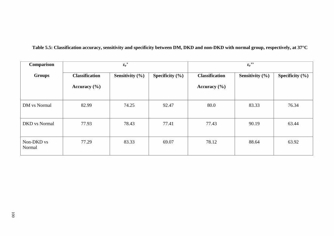
10

0


Comparison

Groups

εr’ εr’’

Classification

Accuracy (%)


Accuracy (%)


DM vs Normal 82.99 74.25 92.47 80.0 83.33 76.34

DKD vs Normal 77.93 78.43 77.41 77.43 90.19 63.44

Non-DKD vs

Normal

77.29 83.33 69.07 78.12 88.64 63.92

101

At 25°C, classification model obtained 84.02%, 81.96% and 79.30% accuracy to

distinguish DM, DKD and non-DKD, respectively, from the normal group using urinary

dielectric constant. Meanwhile, loss factor produced classification accuracies at 77.20%,

75.92% and 71.80% to classify DM, DKD and non-DKD, respectively from the normal

group. Overall, dielectric constant produced higher classification accuracies than loss

factor except for classification between non-DKD and normal group at 37°C. The

highest classification accuracies were observed at 30°C.

5.4.3 Three-group Classifications

5.4.3.1 Classification of DM vs DKD vs normal

Table 5.6 and 5.7 show the confusion matrix of the classifications for urinary

dielectric properties among DM, DKD and normal group at 25°C, 30°C and 37°C. The

classification model showed overall prediction accuracy of 67.0%, 67.64% and 65.55%

using urinary dielectric constant at 25°C, 30°C and 37°C, respectively. Urinary loss

factor produced 61.49%, 66.02% and 61.79% accuracy at 25°C, 30°C and 37°C,

respectively. Urinary dielectric constant produced higher classification accuracies than

loss factor. The highest classification accuracy was shown at 30°C. The overall

deviation of accuracies was determined at about 2~5% across temperatures.

10

2

Table 5.6: Confusion matrix for the classification of urinary dielectric constant among DM, DKD and normal group at 25°C, 30°C and

37°C

25°C 30°C 37°C

DM DKD Normal Accuracy

(%)


(%)


(%)

DM 54 36 12 52.94 55 41 6 53.92 54 34 14 52.94

DKD 12 69 21 67.65 20 71 11 69.61 18 73 11 71.56

Normal 5 14 78 80.41 8 12 77 79.38 6 21 70 72.16

Overall Prediction Accuracy 67.0 67.64 65.55

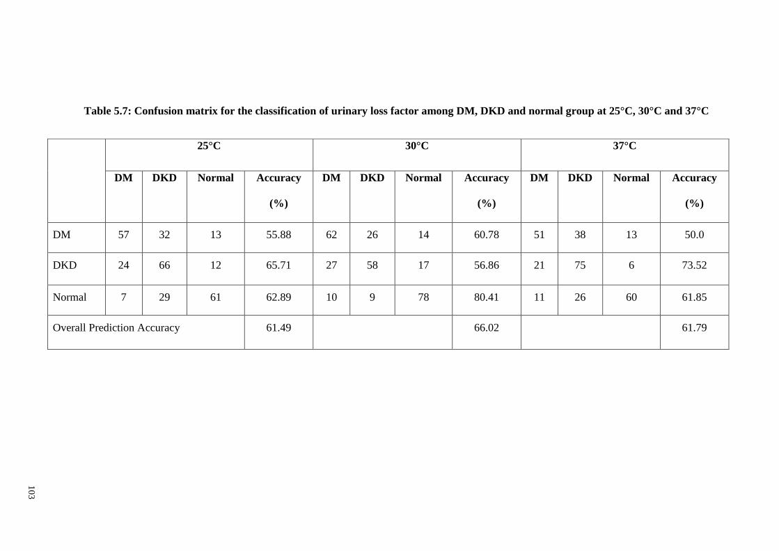
10

3

Table 5.7: Confusion matrix for the classification of urinary loss factor among DM, DKD and normal group at 25°C, 30°C and 37°C

25°C 30°C 37°C


(%)


(%)


(%)

DM 57 32 13 55.88 62 26 14 60.78 51 38 13 50.0

DKD 24 66 12 65.71 27 58 17 56.86 21 75 6 73.52

Normal 7 29 61 62.89 10 9 78 80.41 11 26 60 61.85


104

5.4.3.3 Classification of DM vs non-DKD vs normal

Tables 5.8 and 5.9 show the confusion matrix for the classification of urinary

dielectric properties among DM, non-DKD and normal groups at 25°C, 30°C and 37°C.

The classification model showed overall prediction accuracy of 62.14%, 63.68% and

64.50% using urinary dielectric constant at 25°C, 30°C and 37°C, respectively. Urinary

loss factor produced 59.20%, 63.87% and 63.22% accuracy at 25°C, 30°C and 37°C,

respectively. Overall, urinary dielectric constant showed higher classification accuracies

than loss factor except for classification at 30°C that had deviation <0.5 %.

10

5

Table 5.8: Confusion matrix for the classification of urinary dielectric constant among DM, non-DKD and normal group at 25°C, 30°C and

37°C

25°C 30°C 37°C

DM Non-

DKD

Normal Accuracy

(%)

DM Non-

DKD

Normal Accuracy

(%)

DM Non-

DKD

Normal Accuracy

(%)

DM 42 48 12 41.18 58 37 7 56.86 46 41 15 45.10

Non-DKD 14 94 22 72.31 30 86 14 66.15 13 103 14 79.23

Normal 3 23 71 72.92 5 26 66 68.04 6 24 67 69.07


10

6

Table 5.9: Confusion matrix for the classification of urinary loss factor among DM, non-DKD and normal group at 25°C, 30°C and 37°C

25°C 30°C 37°C

DM Non-

DKD

Normal Accuracy

(%)

DM Non-

DKD

Normal Accuracy

(%)

DM Non-

DKD

Normal Accuracy

(%)

DM 47 43 12 46.07 51 34 17 50.0 53 31 18 51.96

Non-DKD 12 96 22 73.84 18 101 11 77.69 16 100 14 76.90

Normal 8 34 55 57.70 7 28 62 63.92 7 31 59 60.82


107

5.4.3.5 Classification of DKD vs non-DKD vs normal

Tables 5.10 and 5.11 show the confusion matrix for the classification of urinary

dielectric properties among DKD, non-DKD and normal groups at 25°C, 30°C and

37°C. The classification model showed prediction accuracy of 60.92%, 61.12% and

59.63% using urinary dielectric constant at 25°C, 30°C and 37°C, respectively. As for

urinary loss factor, the classification accuracy was reported at 60.27%, 61.23% and

60.41% at 25°C, 30°C and 37°C, respectively. Again, the highest classification accuracy

was achieved at 30°C (61.23%).

10

8

Table 5.10: Confusion matrix for the classification of urinary dielectric constant among DKD, non-DKD and normal group at 25°C, 30°C and

37°C.

25°C 30°C 37°C

DKD Non-

DKD

Normal Accuracy

(%)

DKD Non-

DKD

Normal Accuracy

(%)

DKD Non-

DKD

Normal Accuracy

(%)

DKD 54 40 8 52.94 58 38 6 56.86 49 44 9 48.04

Non-DKD 32 83 15 63.85 39 72 19 55.38 34 83 13 63.85

Normal 16 17 64 65.98 12 16 69 71.13 13 19 65 67.01


10

9

Table 5.11: Confusion matrix for the classification of urinary loss factor among DKD, non-DKD and normal group at 25°C, 30°C and

37°C.

25°C 30°C 37°C

DKD Non-

DKD

Normal Accuracy

(%)

DKD Non-

DKD

Normal Accuracy

(%)

DKD Non-

DKD

Normal Accuracy

(%)

DKD 52 42 8 50.98 59 35 8 56.19 53 45 4 51.96

Non-DKD 40 79 11 60.76 32 84 14 64.62 38 85 7 65.38

Normal 12 18 67 69.07 11 25 61 62.88 12 23 62 63.91


110

5.5 Discussion

5.5.1 Effect of Temperature in Classifications

In fact, urine temperature may vary between the body (37°C) and room temperature

(25°C) in the process of collection to measurement. Temperature variation is an

important factor that affects the dielectric properties. Overall, the highest classification

accuracy was shown at 30°C for two-group and three-group classifications. The

maximum accuracy deviation was about 8% across temperatures of 25°C, 30°C and

37°C. Urinary dielectric properties changed with temperature, due to the stretching of

intramolecular hydrogen bonds between water molecules of solutions (Ellison, 2007).

Urine is a complex biological solution that consists of different chemical constituents

that are broadly categorised as electrolytes, organic and in-organic compounds. The

combination effects of ionic conductance, molecular Brownian movement and hydrogen

bonds increased with temperature in urine. However, randomising the agitation of

molecules at high temperature reduced the significant effect of the biomaterials present

in urine that could affect the classification accuracy. The classifications of urinary

dielectric behaviour were optimal at 30°C for urine, while the accuracies decreased

when the temperature reached 37°C.

5.5.2 Two-group Classifications

In two-group classifications, the highest classification accuracies for urinary

dielectric properties were obtained to differentiate DM from normal group. The

deviations were about 2~5% in comparison between DM and CKD two-group

classifications of urinary dielectric properties. Overall, the classification model

produced considerably high accuracies, which appear to be sufficient to classify the

urinary dielectric properties as a function between disease and normal group. These

findings suggest the existence of unique behaviours related to urinary dielectric

properties between normal and disease conditions at microwave frequency between

111

1GHz and 50GHz. The presence of glycosuria and proteinuria in DM and CKD subject

groups, respectively, significantly affects the behaviour of urinary dielectric properties.

5.5.3 Three-group Classifications

In three-group classifications, the lowest accuracy was obtained when classifying the

urinary dielectric properties of DM subjects among CKD and normal subject groups.

High misclassifications in prediction output of DM subjects were classified as CKD

subjects. The highest misclassification was found in about 41 and 48 subjects from a

total of 102 DM subjects who were classified in the DKD and non-DKD groups,

respectively. The confusion classification between DM and CKD group was about 35 ~

45%. It may be due to the possible existence of DM subjects with high risk of getting

CKD, who have absence of clinical symptoms with estimated glomerular filtration rate

(eGFR) < 90 ml/min per 1.73m2. As reported by Zürbig et al. (2009), initial

pathophysiological changes in kidneys resulted in different urinary constituents such as

micro-albuminuria as a potential biomarker for early stage of CKD. Based on the

pathological changes, the measurement of urinary dielectric properties would potentially

be able to distinguish diabetic subjects with high risk of CKD. However, this study

remains limited for changes in urinary dielectric properties for albuminuria. Meanwhile,

Alkhalaf et al. (2010) discovered that different biomarkers were found between Type 1

and 2 DM patients due to the different pathophysiology of the particular DKD. Type 1

DM still remains a challenge in this study and requires future investigation.

5.5.4 Comparison Accuracy between Classification Methods

Table 5.12 and Table 5.13 show the comparison of accuracies between threshold and

SVM classification method for urinary dielectric properties. Overall, classification

accuracies produced by SVM were significantly higher than the threshold method for

25°C, 30°C and 37°C. The accuracy deviations were >10% in comparison between the

112

two classification methods except for CKD vs normal group at 37°C. This shows that

SVM enhanced the accuracy of urinary dielectric properties measurement in

distinguishing DM and CKD, respectively, from normal subjects.


classification method for urinary dielectric constant.

Comparison

Groups

Threshold SVM

25°C 30°C 37°C 25°C 30°C 37°C

DM vs

Normal

72.0 77.08 66.67 84.02 88.72 82.99

CKD vs

Normal

59.72 68.67 79.52 79.30 79.30 77.29


classification methods for urinary loss factor.

Comparison

Groups

Threshold SVM

25°C 30°C 37°C 25°C 30°C 37°C

DM vs

Normal

54.90 69.39 66.67 77.20 80.51 80.0

CKD vs

Normal

72.29 69.88 51.81 71.80 79.30 78.12

113

5.6 Summary

In this chapter, the urinary dielectric properties of Type 2 DM, CKD and normal

group were classified by using the SVM classification model at microwave frequency

from 1 GHz to 50 GHz. The CKD group was further categorised into DKD and non-

DKD for classification. Differences in urinary dielectric properties were observed

between DKD and non-DKD compared to the normal group, and between DKD and

non-DKD groups. Two-group and three-group classifications were conducted. In two-

group classifications, the highest classification accuracy was achieved at 88.72% for

differentiating DM from the normal group. As for the three-group classifications, the

highest accuracy was achieved at 67.64%. The effect of temperature in the classification

of urinary dielectric properties was determined. The highest classification accuracy was

obtained at 30°C for two-group and three-group classifications. SVM classification

enhanced the accuracy of urinary dielectric properties measurement in distinguishing

Type 2 DM and CKD from normal subjects.

114

CHAPTER 6: CONCLUSIONS AND RECOMMENDATIONS

6.1 Conclusions

This study investigated the urinary dielectric properties of Type 2 DM, CKD and

normal subjects using the open-ended coaxial probe technique at microwave frequency

between 0.2 GHz and 50 GHz. Dielectric constant increased with glycosuria level of

more than 5 g/L (0.5%) at low frequencies, while correlated positively with glycosuria

level at frequencies above 40 GHz. Loss factor correlated negatively with glycosuria

level at frequencies above 15 GHz. Relaxation frequency shifted towards lower values

with higher glycosuria levels. The strongest statistically significant differences in

urinary dielectric properties across different glycosuria levels were reported at 25°C.

The urinary dielectric properties of CKD subjects were higher and lower than those

of normal subjects at frequencies below and above the ―cross-over‖ frequency points,

respectively. The strongest statistically significant differences in the urinary dielectric

properties of CKD subjects compared with normal subjects were reported at 37°C.

Urinary dielectric properties correlated positively and negatively with proteinuria level

at frequencies below and above the ―cross-over‖ frequency point, respectively.

The experimental data closely matched the single-pole Debye model. The urinary

relaxation dispersion and relaxation time increased with the glycosuria and proteinuria

levels, respectively, while decreased with temperature. As for static conductivity, it

increased with proteinuria levels higher than 1.5 g/L.

Classifications of urinary dielectric behaviour of DM, CKD and normal groups were

conducted using the SVM-based classification model at microwave frequencies from 1

GHz to 50 GHz. In two-group classifications, the highest classification accuracy was

achieved at 88.72%, 84.10% and 79.38% for differentiating DM, DKD and non-DKD

groups, respectively, from the normal group. The highest accuracy was achieved at

115

67.64% in three-group classifications. The temperature of 30°C was found to be optimal

for the classification of urinary dielectric behaviour, compared to 25°C and 37°C. SVM

enhanced the classification accuracy of urinary dielectric properties measurement in

distinguishing DM and CKD from normal subjects. This study demonstrated the

potential diagnostic and prognostic value of urinary dielectric properties for Type 2 DM

and CKD.

6.2 Recommendations

At the current stage, the differences in urinary dielectric properties of glycosuria and

proteinuria, involving DM and CKD, respectively, are insufficient for applying

dielectric spectroscopy as a diagnostic or monitoring tool. Cross-comparison of

dielectric techniques may be required for determining the validation of differences

between subject groups. Collection and measurement of urine must be particularly

careful to avoid contamination that may affect the results. Future studies will require

larger patient groups with broader glycosuria or proteinuria variability, and

measurement taken over a wider microwave frequency range. In this study, the urinary

dielectric properties were found would potentially be able to distinguish diabetic

subjects with high risk of CKD. However, this study highlights the need for future

investigation of the changes in urinary dielectric properties changes with albuminuria.

On the other hand, different biomarkers reported between Type 1 and 2 DM patients

showed different pathophysiology of the resulting diabetic kidney disease (Alkhalaf et

al., 2010). This poses a challenge for future investigation into dielectric properties for

Type 1 DM.

Moreover, future studies on correlations between serum glucose level and creatinine

with urinary dielectric properties are recommended. This is certainly important to

116

determine the indirect impact of serum glucose or creatinine that causes differences in

urine composition, which subsequently changes urinary dielectric properties.

The measurement of dielectric properties could be extended to other diseases, such as

leukaemia, bladder stone, bladder cancer and oral cancer that strongly require clinical

determination in biological solutions. Dielectric properties would work as powerful

parameters to determine variations of biomaterials in a solution for clinical utility.

117

REFERENCES

Abdalla, S. (2011). Effect of erythrocytes oscillations on dielectric properties of human

diabetic-blood. AIP Advances, 1(1), 012104-012115.

Abdalla, S., Al-Ameer, S., & Al-Magaishi, S. (2010). Electrical properties with

relaxation through human blood. Biomicrofluidics, 4(3), 034101-034116.

Agilent Technologies. (2005). Basics of measuring the dielectric properties of materials.

Retrieved from http://cp.literature.agilent.com/

Agilent Technologies. (2012). Agilent 85070e dielectric probe kit 200 mhz to 50 ghz.

Retrieved from http://cp.literature.agilent.com/litweb/pdf/5989-0222EN.pdf

Alabaster, C. M. (2004). The microwave properties of tissue and other lossy dielectrics.

(Doctoral thesis, Cranfield University, England). Retrived from

https://dspace.lib.cranfield.ac.uk/handle/1826/251

Alison, J., & Sheppard, R. (1993). Dielectric properties of human blood at microwave

frequencies. Physics in Medicine and Biology, 38(7), 971-978.

Alkhalaf, A., Zürbig, P., Bakker, S. J., Bilo, H. J., Cerna, M., Fischer, C., . . . Mischak,

H. (2010). Multicentric validation of proteomic biomarkers in urine specific for

diabetic nephropathy. Plos One, 5(10), e13421-e13431.

American Diabetes Association. (1994). Self-monitoring of blood glucose. Diabetes

Care, 17(1), 81-86.

American Diabetes Association. (1998). Tests of glycemia in diabetes. Diabetes Care,

21(Supplement 1), S69-S71.

American Diabetes Association. (2010). Standards of medical care in diabetes—2010.

Diabetes Care, 33(Supplement 1), S11-S61.

American Diabetes Association. (2014). Statistics about diabetes. National Diabetes

Statistics Report. Retrieved from http://www.diabetes.org/diabetes-

basics/statistics/

Arai, M., Binner, J., & Cross, T. (1995). Correction of errors owing to thermal

elongation of high temperature coaxial probe for microwave permittivity

measurement. Electronics Letters, 31(14), 1138-1139.

Atkins, R. C., Briganti, E. M., Lewis, J. B., Hunsicker, L. G., Braden, G., de Crespigny,

P. J. C., . . . Wiegmann, T. B. (2005). Proteinuria reduction and progression to

renal failure in patients with type 2 diabetes mellitus and overt nephropathy.

American Journal of Kidney Diseases, 45(2), 281-287.

Ban, H. J., Heo, J. Y., Oh, K. S., & Park, K. J. (2010). Identification of type 2 diabetes-

associated combination of snps using support vector machine. BMC Genetics,

11, 26-36.

http://cp.literature.agilent.com/

http://cp.literature.agilent.com/litweb/pdf/5989-0222EN.pdf

http://www.diabetes.org/diabetes-basics/statistics/

http://www.diabetes.org/diabetes-basics/statistics/

118

Barakat, N., Bradley, A. P., & Barakat, M. N. H. (2010). Intelligible support vector

machines for diagnosis of diabetes mellitus. IEEE Transactions on Information

Technology in Biomedicine, 14(4), 1114-1120.

Bassey, C. E., & Cowell, S. (2013). Electrical properties of sucrose solutions for

diabetic applications. Biophysical Journal, 104(2), 688a. doi:

10.1016/j.bpj.2012.11.3802

Ben-Hur, A., & Weston, J. (2010). A user‘s guide to support vector machines. Methods

in Molecular Biology, 609, 223-239. doi: 10.1007/978-1-60327-241-4_13.

Blackham, D. V., & Pollard, R. D. (1997). An improved technique for permittivity

measurements using a coaxial probe. IEEE Transactions on Instrumentation and

Measurement, 46(5), 1093-1099.

Boresch, S., Höchtl, P., & Steinhauser, O. (2000). Studying the dielectric properties of a

protein solution by computer simulation. The Journal of Physical Chemistry B,

104(36), 8743-8752.

Buchner, R., Hefter, G. T., & May, P. M. (1999). Dielectric relaxation of aqueous NaCl

solutions. The Journal of Physical Chemistry A, 103(1), 1-9.

Bush Jr, W., Amis Jr, E., Bigongiari, L., Bluth, E., Choyke, P., Fritzsche, P., . . . Segal,

A. (2000). Radiologic investigation of causes of renal failure. American college

of radiology. ACR appropriateness criteria. Radiology, 215, 713-720.

Caduff, A., Hirt, E., Feldman, Y., Ali, Z., & Heinemann, L. (2003). First human

experiments with a novel non-invasive, non-optical continuous glucose

monitoring system. Biosensors and Bioelectronics, 19(3), 209-217.

Campbell, A., & Land, D. (1992). Dielectric properties of female human breast tissue

measured in vitro at 3.2 GHz. Physics in Medicine and Biology, 37(1), 193.

Chan, A., Swaminathan, R., & Cockram, C. (1989). Effectiveness of sodium fluoride as

a preservative of glucose in blood. Clinical chemistry, 35(2), 315-317.

Chang, C. C., & Lin, C. J. (2011). Libsvm: A library for support vector machines. ACM

Transactions on Intelligent Systems and Technology (TIST), 2(3), 27.

Chen, L. F., Ong, C., Neo, C., Varadan, V., & Varadan, V. K. (2004). Microwave

electronics: Measurement and materials characterization. Chichester, England:

John Wiley & Sons.

Cole, K. S., & Cole, R. H. (1942). Dispersion and absorption in dielectrics II. Direct

current characteristics. The Journal of Chemical Physics, 10(2), 98-105.

Craig, D. (1995). Dielectric analysis of pharmaceutical systems. Oxford, United

Kingdom: Taylor & Francis.

De los Santos, J., Garcia, D., & Eiras, J. A. (2003). Dielectric characterization of

materials at microwave frequency range. Materials Research, 6(1), 97-101.

119

Desouky, O. (2009). Rheological and electrical behavior of erythrocytes in patients with

diabetes mellitus. Romanian Journal of Biophysics, 19, 239-250.

Ellison, W. (2007). Permittivity of pure water, at standard atmospheric pressure, over

the frequency range 0–25THz and the temperature range 0–100 C. Journal of

Physical and Chemical Reference Data, 36(1), 1-18.

Ellison, W., Lamkaouchi, K., & Moreau, J.-M. (1996). Water: A dielectric reference.

Journal of molecular liquids, 68(2), 171-279.

Epstein, F. H., Remuzzi, G., & Bertani, T. (1998). Pathophysiology of progressive

nephropathies. The New England Journal of Medicine, 339(20), 1448-1456.

Feisul, M., & Azmi, S. (2012). Management of chronic kidney disease in adults.

National Diabetes Registry Report. Retrieved from

http://www.msn.org.my/Doc/PublicDoc_PB/CPGManagementOfChronicKidney

Disease.pdf

Fernández, D. P., Mulev, Y., Goodwin, A., & Sengers, J. L. (1995). A database for the

static dielectric constant of water and steam. Journal of Physical and Chemical

Reference Data, 24(1), 33-70.

Ferry, J. D., & Oncley, J. (1938). Studies of the dielectric properties of protein

solutions. II. The water-soluble proteins of normal horse serum1, 2. Journal of

the American Chemical Society, 60(5), 1123-1132.

Fuchs, K., & Kaatze, U. (2001). Molecular dynamics of carbohydrate aqueous solutions.

Dielectric relaxation as a function of glucose and fructose concentration. The

Journal of Physical Chemistry B, 105(10), 2036-2042.

Gabriel, C., Gabriel, S., & Corthout, E. (1996a). The dielectric properties of biological

tissues: I. Literature survey. Physics in Medicine and Biology, 41(11), 2231-

2249.

Gabriel, C., & Peyman, A. (2006). Dielectric measurement: Error analysis and

assessment of uncertainty. Physics in Medicine and Biology, 51(23), 6033-6046.

Gabriel, S., Lau, R., & Gabriel, C. (1996b). The dielectric properties of biological

tissues: II. Measurements in the frequency range 10 hz to 20 GHz. Physics in

Medicine and Biology, 41(11), 2251-2269.

Gabriel, S., Lau, R., & Gabriel, C. (1996c). The dielectric properties of biological

tissues: III. Parametric models for the dielectric spectrum of tissues. Physics in

Medicine and Biology, 41(11), 2271.

Ganji, M. F., & Abadeh, M. S. (2011). A fuzzy classification system based on ant

colony optimization for diabetes disease diagnosis. Expert Systems with

Applications, 38(12), 14650-14659.

Ghiggeri, G. M., Candiano, G., Delfino, G., & Queirolo, C. (1985). Electrical charge of

serum and urinary albumin in normal and diabetes human. Kidney International,

28, 168-177.

http://www.msn.org.my/Doc/PublicDoc_PB/CPGManagementOfChronicKidneyDisease.pdf

http://www.msn.org.my/Doc/PublicDoc_PB/CPGManagementOfChronicKidneyDisease.pdf

120

Goldstein, D. E., Little, R. R., Lorenz, R. A., Malone, J. I., Nathan, D., Peterson, C. M.,

& Sacks, D. B. (2004). Tests of glycemia in diabetes. Diabetes Care, 27(7),

1761-1773.

Gonzalez, C. A., Valencia, J. A., Mora, A., Gonzalez, F., Velasco, B., Porras, M. A., . . .

Cordero, S. (2013). Volumetric electromagnetic phase-shift spectroscopy of

brain edema and hematoma. Plos One, 8(5), e63223-e63233.

Grant, E. H., Keefe, S. E., & Takashima, S. (1968). Dielectric behavior of aqueous

solutions of bovine serum albumin from radiowave to microwave frequencies.

The Journal of Physical Chemistry, 72(13), 4373-4380.

Grant, J., Clarke, R., Symm, G., & Spyrou, N. M. (1989). A critical study of the open-

ended coaxial line sensor technique for rf and microwave complex permittivity

measurements. Journal of Physics E: Scientific Instruments, 22(9), 757.

Gregory, A. P., & Clarke, R. (2001). Tables of the complex permittivity of dielectric

reference liquids at frequencies up to 5 GHz. Teddington, Scotland: National

Physical Laboratory.

Grewal, P. K., & Golnaraghi, F. (2014). Pilot study: Electrical impedance based tissue

classification using support vector machine classifier. IET Science, Measurement

& Technology, 8(6), 579-587.

Gronwald, W., Klein, M. S., Zeltner, R., Schulze, B. D., Reinhold, S. W., Deutschmann,

M., . . . Eckardt, K. U. (2011). Detection of autosomal dominant polycystic

kidney disease by nmr spectroscopic fingerprinting of urine. Kidney

International, 79(11), 1244-1253.

Haubitz, M., Wittke, S., Weissinger, E. M., Wellen, M., Ruppech, H. D., Floege, J. U., .

. . Michack, H. (2005). Urine protein patterns can serve as diagnostic tools in

patients with IgA nephropathy. Kidney International, 67(6), 2313-2320.

Hayashi, Y., Livshits, L., Caduff, A., & Feldman, Y. (2003). Dielectric spectroscopy

study of specific glucose influence on human erythrocyte membranes. Journal of

Physics D: Applied Physics, 36(4), 369-374.

Haykin, S., & Network, N. (2004). Neural networks a comprehensive foundation (2nd

ed.). New Jersey, United States: Prentice Hall.

Höchtl, P., Boresch, S., & Steinhauser, O. (2000). Dielectric properties of glucose and

maltose solutions. The Journal of Chemical Physics, 112(22), 9810-9821.

Horiuchi, T., Takahashi, M., Kikuchi, J., Yokoyama, S., & Maeda, H. (2005). Effect of

dielectric properties of solvents on the quality factor for a beyond 900mhz

cryogenic probe model. Journal of Magnetic Resonance, 174(1), 34-42.

IBM Corp. (2012). SPSS statistics for windows [computer software]. New York, NY:

Armonk.

121

Icier, F., & Baysal, T. (2004). Dielectrical properties of food materials—2:

Measurement techniques. Critical reviews in food science and nutrition, 44(6),

473-478.

Imbeault, P., Prins, J. B., Stolic, M., Russell, A. W., O‘Moore-Sullivan, T., Després, J.-

P., . . . Tremblay, A. (2003). Aging per se does not influence glucose

homeostasis in vivo and in vitro evidence. Diabetes Care, 26(2), 480-484.

International Dibates Federation. (2016). Diabetes in Malaysia. Retrieved from

http://www.idf.org/membership/wp/malaysia

Iseki, K., Kinjo, K., Iseki, C., & Takishita, S. (2004). Relationship between predicted

creatinine clearance and proteinuria and the risk of developing esrd in okinawa,

japan. American Journal of Kidney Diseases, 44(5), 806-814.

Ishani, A., Grandits, G. A., Grimm, R. H., Svendsen, K. H., Collins, A. J., Prineas, R. J.,

& Neaton, J. D. (2006). Association of single measurements of dipstick

proteinuria, estimated glomerular filtration rate, and hematocrit with 25-year

incidence of end-stage renal disease in the multiple risk factor intervention trial.

Journal of the American Society of Nephrology, 17(5), 1444-1452.

Jafar, T. H., Stark, P. C., Schmid, C. H., Landa, M., Maschio, G., Marcantoni, C., . . .

Ruggenenti, P. (2001). Proteinuria as a modifiable risk factor for the progression

of non-diabetic renal disease. Kidney International, 60(3), 1131-1140.

Jaspard, F., Nadi, M., & Rouane, A. (2003). Dielectric properties of blood: An

investigation of haematocrit dependence. Physiological Measurement, 24(1),

137-147.

Johri, G., & Roberts, J. (1990). Study of the dielectric response of water using a

resonant microwave cavity as a probe. Journal of Physical Chemistry, 94(19),

7386-7391.

Kaatze, U. (1989). Complex permittivity of water as a function of frequency and

temperature. Journal of Chemical and Engineering Data, 34(4), 371-374.

Kaatze, U. (2007). Reference liquids for the calibration of dielectric sensors and

measurement instruments. Measurement Science and Technology, 18(4), 967.

Kabadi, U. M., O'Connell, K. M., Johnson, J., & Kabadi, M. (1994). The effect of

recurrent practice at home on the acceptability of capillary blood glucose

readings: Accuracy of self blood glucose testing. Diabetes Care, 17(10), 1110-

1114.

Kanwar, Y. S., Wada, J., Sun, L., Xie, P., Wallner, E. I., Chen, S., . . . Danesh, F. R.

(2008). Diabetic nephropathy: Mechanisms of renal disease progression.

Experimental Biology and Medicine, 233(1), 4-11.

Karabatak, M., & Ince, M. C. (2009). An expert system for detection of breast cancer

based on association rules and neural network. Expert Systems with

Applications, 36(2), 3465-3469.

122

Karacolak, T., Moreland, E. C., & Topsakal, E. (2013). Cole–cole model for glucose‐dependent dielectric properties of blood plasma for continuous glucose

monitoring. Microwave and Optical Technology Letters, 55(5), 1160-1164.

Kerhet, A., Raffetto, M., Boni, A., & Massa, A. (2006). A svm-based approach to

microwave breast cancer detection. Engineering Applications of Artificial

Intelligence, 19(7), 807-818.

Kim, S., Kim, J., Babajanyan, A., Lee, K., & Friedman, B. (2009). Noncontact

characterization of glucose by a waveguide microwave probe. Current Applied

Physics, 9(4), 856-860.

Kistler, A. D., Mischak, H., Poster, D., Dakna, M., Wüthrich, R. P., & Serra, A. L.

(2009). Identification of a unique urinary biomarker profile in patients with

autosomal dominant polycystic kidney disease. Kidney International, 76(1), 89-

96.

Komarov, V., Wang, S., & Tang, J. (2005). Encyclopedia of rf and microwave

engineering. New York: John Wiley and Sons.

Kraszewski, A., Stuchly, M. A., & Stuchly, S. S. (1983). Ana calibration method for

measurements of dielectric properties. Instrumentation and Measurement, IEEE

Transactions on, 32(2), 385-387.

Kreisberg, R. A. (1978). Diabetic ketoacidosis: New concepts and trends in

pathogenesis and treatment. Annals of internal medicine, 88(5), 681-695.

Ladenson, J., Sonnenwirth, A., & Jarett, L. (1980). Nonanalytical sources of variation in

clinical chemistry results. In A.C. Sonnenwirth & L. Jarett (Eds.), Clinical

laboratory methods and diagnosis (pp. 149-192). Maryland, United States: CV

Mosby.

Lascano, M. E., & Poggio, E. D. (2010). Kidney function assessment by creatinine-

based estimation equations. Disease Management. Retrieved from

http://www.clevelandclinicmeded.com/medicalpubs/diseasemanagement/nephrol

ogy/kidney-function/Default.htm

Laufer, S., & Rubinsky, B. (2009). Tissue characterization with an electrical

spectroscopy svm classifier. IEEE Transactions on Biomedical Engineering,

56(2), 525-528.

Lea, J., Greene, T., Hebert, L., Lipkowitz, M., Massry, S., Middleton, J., . . . Bakris, G.

L. (2005). The relationship between magnitude of proteinuria reduction and risk

of end-stage renal disease: Results of the african american study of kidney

disease and hypertension. Archives of Internal Medicine, 165(8), 947-953.

Liao, X., Raghavan, V. G. S., Meda, V., & Yaylayan, V. A. (2001). Dielectric

properties of supersaturated d-glucose aqueous solution at 2450MHz. Journal of

Microwave Power and Electromagnetics Energy, 36(3), 131-138.

Lonappan, A. (2012). Novel method of detecting pregnancy using microwaves. Journal

of Electromagnetic Analysis and Applications, 4(8), 340-343.

http://www.clevelandclinicmeded.com/medicalpubs/diseasemanagement/nephrology/kidney-function/Default.htm

http://www.clevelandclinicmeded.com/medicalpubs/diseasemanagement/nephrology/kidney-function/Default.htm

123

Lonappan, A., Bindu, G., Thomas, V., Jacob, J., Rajasekaran, C., & Mathew, K. T.

(2007a). Diagnosis of diabetes mellitus using microwaves. Journal of

Electromagnetic Waves and Applications, 21(10), 1393-1401.

Lonappan, A., Hamsakkutty, V., Bindu, G., Jacob, J., Thomas, V., & Mathew, K.

(2004). Dielectric properties of human urine at microwave frequencies.

Microwave and Optical Technology Letters, 42(6), 500-503.

Lonappan, A., Kumar, P., Bindu, G., Thomas, V., Mathew, K. T., & (2006a).

Qualitative analysis of human semen using microwaves. Paper presented at the

Progress in Electromagnetics Research Symposium, Cambridge, USA.

Lonappan, A., Rajasekaran, C., Thomas, V., Bindu, G., & Mathew, K. T. (2007b).

Determination of pregnancy using microwaves. Microwave and Optical

Technology Letters, 49(4), 786-788. doi: 10.1002/mop.22279

Lonappan, A., Rajasekharam, C., Thomas, V., Bindu, G., & Mathew, K. T. (2007c).

Dielectric properties of human colostrum at microwave frequencies. Journal of

Microwave Power and Electromagnetic Energy, 41(2), 33-38.

Lonappan, A., Thomas, V., Bindu, G., Hamsakutty, V., & Mathew, K. T. (2006b).

Analysis of human breast milk at microwave frequencies. Progress In

Electromagnetics Research, 60, 179-185.

Lonappan, A., Thomas, V., Bindu, G., Rajasekaran, C., & Mathew, K. T. (2007d).

Nondestructive measurement of human blood at microwave frequencies. Journal

of Electromagnetic Waves and Application, 21(8), 1131-1139. doi:

10.1163/156939307781749740

Maritim, A., Sanders, R., & Watkins, r. J. (2003). Diabetes, oxidative stress, and

antioxidants: A review. Journal of biochemical and molecular toxicology, 17(1),

24-38.

Mathworks. (2011). Matlab and statistics toolbox release 2011a [computer software].

Massachusetts, MA: Natick.

Matyushov, D. V. (2012). On the theory of dielectric spectroscopy of protein solutions.

Journal of Physics: Condensed Matter, 24(32), 325105-325120.

Meriakri, V., Chigrai, E., Kim, D., Nikitin, I., Pangonis, L., Parkhomenko, M., & Won,

J. (2007a). Dielectric properties of glucose solutions in the millimetre-wave

range and control of glucose content in blood. Measurement Science and

Technology, 18(4), 1-6.

Meriakri, V. V., EEChigrai, Nikitin, D. P., LIPangonis, Parkhomenko, M., & HWon, J.

(2007b). Dielectric properties of glucose solutions in the millimetre-wave range

and control of glucose content in blood. Measurement Science and Technology,

18, 1-6.

Metaxas, A. a., & Meredith, R. J. (1983). Industrial microwave heating. London,

England: The Institution of .Engineering and Technology.

124

Michie, D., Spiegelhalter, D. J., & Taylor, C. C. (1994). Machine learning, neural and

statistical classification. New York, United States: Overseas Press.

Monnier, L., Mas, E., Ginet, C., Michel, F., Villon, L., Cristol, J.-P., & Colette, C.

(2006). Activation of oxidative stress by acute glucose fluctuations compared

with sustained chronic hyperglycemia in patients with type 2 diabetes. The

Journal of the American Medical Association, 295(14), 1681-1687.

Nandi, N., & Bagchi, B. (1998). Anomalous dielectric relaxation of aqueous protein

solutions. The Journal of Physical Chemistry A, 102(43), 8217-8221.

Nelson, S. O. (1996). Review and assessment of radio-frequency and microwave energy

for stored-grain insect control. Transactions of the ASAE, 39(4), 1475-1484.

Nörtemann, K., Hilland, J., & Kaatze, U. (1997). Dielectric properties of aqueous nacl

solutions at microwave frequencies. The Journal of Physical Chemistry A,

101(37), 6864-6869.

O‘Rourke, A. P., Lazebnik, M., Bertram, J. M., Converse, M. C., Hagness, S. C.,

Webster, J. G., & Mahvi, D. M. (2007). Dielectric properties of human normal,

malignant and cirrhotic liver tissue: In vivo and ex vivo measurements from 0.5

to 20 GHz using a precision open-ended coaxial probe. Physics in Medicine and

Biology, 52(15), 4707-4719.

Oncley, J. (1938). Studies of the dielectric properties of protein solutions. I.

Carboxyhemoglobin1, 2. Journal of the American Chemical Society, 60(5),

1115-1123.

Park, J.-H., Kim, C.-S., Choi, B.-C., & Ham, K.-Y. (2003). The correlation of the

complex dielectric constant and blood glucose at low frequency. Biosensors and

Bioelectronics, 19(4), 321-324.

Pekkanen, J., Tuomilehto, J., & Group, D. S. (1999). Consequences of the new

diagnostic criteria for diabetes in older men and women. Diabetes Care. 22(10),

1667-1671.

Pethig, R., & Kell, B. (1987). The passive electrical properties of biological systems:

Their significance in physiology, biophysics and biotechnology. Physics in

Medicine and Biology, 32(8), 933-970.

Peyman, A., & Gabriel, C. (2010). Cole-cole parameters for the dielectric properties of

porcine tissues as a function of age at microwave frequencies. Physics in

Medicine and Biology, 55(15), N413-419.

Peyman, A., & Gabriel, C. (2012). Dielectric properties of porcine glands, gonads and

body fluids. Physics in Medicine and Biology, 57(19), N339-N344.

Polat, K., Güneş, S., & Arslan, A. (2008). A cascade learning system for classification

of diabetes disease: Generalized discriminant analysis and least square support

vector machine. Expert Systems with Applications, 34(1), 482-487.

125

Rajasekharan, C., Girishkumar, C., Lonappan, A., Mathew, A. J., & Mathew, K. T.

(2010). Diagnostic value of microwaves in neurological disorder. Journal of

Microwave Power and Electromagnetic Energy, 44(3), 139-143.

Raveendranath, U., Kumar, S. B., Mathew, S., & Mathew, K. T. (1998). Micowave

diagnosis of diabetes in humanbeings using cavity perturbation technique. Paper

presented at the Microwave and Millimeter Wave Technology Proceedings,

Beijing, China.

Raveendranath, U., & Mathew, K. (1996). The study of the dielectric behaviour of

vapours of water and organic liquids at microwave frequencies. Journal of

molecular liquids, 68(2), 145-156.

Robert, J., Huang, J., & Wang, H. (1993). Temperature dependence of dielectric

relaxation and conductivity of water. Paper presented at the IEEE 11th

International Conference on Conduction and Breakdown in Dielectric Liquids,

Baden-Dattwil, Switzerland.

Rodríguez-Arteche, I., Cerveny, S., Alegría, Á., & Colmenero, J. (2012). Dielectric

spectroscopy in the ghz region on fully hydrated zwitterionic amino acids.

Physical Chemistry Chemical Physics, 14(32), 11352-11362.

Roshan, U., Chikkagoudar, S., Wei, Z., Wang, K., & Hakonarson, H. (2011). Ranking

causal variants and associated regions in genome-wide association studies by the

support vector machine and random forest. Nucleic Acids Research, 39(9), e62-

e62.

Ryynänen, S. (1995). The electromagnetic properties of food materials: A review of the

basic principles. Journal of Food Engineering, 26(4), 409-429.

Sacks, D. B., Arnold, M., Bakris, G. L., Bruns, D. E., Horvath, A. R., Kirkham, M. S., .

. . Nathan, D. M. (2011). Urinary glucose. In D. B. Sacks (Ed.), Guidelines and

recommendations for laboratory management of diabetes mellitus (pp. 21-23).

Washington: National Academy of Clinical Biochemistry.

Salifu, M. O. (2015). Azotemia. Medscape. Retrieved from

http://emedicine.medscape.com/article/238545-overview

Sbrignadello, S., Tura, A., & Ravazzani, P. (2012). Electroimpedance spectroscopy for

the measurement of the dielectric properties of sodium chloride solutions at

different glucose concentrations. Journal of Spectroscopy, 2013, 1-6.

Shim, S., Stemke-Hale, K., Noshari, J., Becker, F. F., & Gascoyne, P. R. (2013).

Dielectrophoresis has broad applicability to marker-free isolation of tumor cells

from blood by microfluidic systems. Biomicrofluidics, 7(1), 011808-011820.

Shini, M. A., Laufer, S., & Rubinsky, B. (2011). Svm for prostate cancer using

electrical impedance measurements. Physiological Measurement, 32(9), 1373-

1387.

http://emedicine.medscape.com/article/238545-overview

126

Smith, R., Lee, S., Komori, H., & Arai, K. (1998). Relative permittivity and dielectric

relaxation in aqueous alcohol solutions. Fluid Phase Equilibria, 144(1), 315-

322.

Smulders, P. F., Buysse, M. G., & Huang, M. D. (2013). Dielectric properties of glucose

solutions in the 0.5–67 ghz range. Microwave and Optical Technology Letters,

55(8), 1916-1917.

Tang, Z., Lee, J. H., Louie, R. F., & Kost, G. J. (2000). Effects of different hematocrit

levels on glucose measurements with handheld meters for point-of-care testing.

Archives of Pathology & Laboratory Medicine, 124(8), 1135-1140.

Topsakal, E., Karacolak, T., & Moreland, E. C. (2011). Glucose-dependent dielectric

properties of blood plasma. Paper presented at the General Assembly and

Scientific Symposium, Istanbul, Turkey.

Tura, A., Sbrignadello, S., Barison, S., Conti, S., & Pacini, G. (2007). Impedance

spectroscopy of solutions at physiological glucose concentrations. Biophysical

Chemistry, 129(2), 235-241.

Uematsu, M., & Franck, E. U. (1980). Static dielectric constant of water and steam.

Journal of Physical and Chemical Reference Data, 9(4), 1297-1307.

Vapnik, V. N. (1995). The nature of statistical learning theory. New York, United

States: Springer-Verlag.

Venkatesh, M. S., & Raghavan, G. S. V. (2005). A overview of dielectric properties

measuring techniques. Canadian Biosystems Engineering, 47, 7.15-17.30.

Wentholt, I., Kulik, W., Michels, R., Hoekstra, J. L., & DeVries, J. (2008). Glucose

fluctuations and activation of oxidative stress in patients with type 1 diabetes.

Diabetologia, 51(1), 183-190.

Wolf, M., Gulich, R., Lunkenheimer, R., & Loid, A. (2012). Relaxation dynamics of

protein solution investigated by dielectric spectroscopy. Proteins and

Proteomics, 1-7.

World Health Organization. (2006). Definition and diagnosis of diabetes mellitus and

intermediate hyperglycaemia: Report of a WHO/IDF consultation. Retrieved

from http://www.who.int/diabetes/publications/diagnosis_diabetes2006/en/.

Yomogida, Y., Iwasaki, T., Matsumoto, M., Mishina, T., & Nozaki, R. (2012). Recent

advances in broadband dielectric spectroscopy (pp. 19-35). Dordrecht, The

Netherlands: Springer.

Zhadobov, M., Augustine, R., Sauleau, R., Alekseev, S., Di Paola, A., Le Quément, C., .

. . Le Dréan, Y. (2012). Complex permittivity of representative biological

solutions in the 2–67 ghz range. Bioelectromagnetics, 33(4), 346-355.

Zürbig, P., Decramer, S., Dakna, M., Jantos, J., Good, D. M., Coon, J. J., . . . Schanstra,

J. P. (2009). The human urinary proteome reveals high similarity between

127

kidney aging and chronic kidney disease. Proteomics, 9(8), 2108-2117. doi:

10.1002/pmic.200800560

128

LIST OF PUBLICATIONS AND PAPERS PRESENTED

i. Mun, P. S., Ting, H. N., Ong, T. A., Wong, C. M., Ng, K. H. & Chong, Y.

B. (2015) A study of dielectric properties of proteinuria between 0.2 and

50 GHz. Plos One, 10(6), e0130011.

129

ii. Mun, P. S., Ting, H. N., Chong, Y. B. & Ong, T. A. (2015) Dielectric

properties of glycosuria at 0.2-50 GHz using microwave spectroscopy.

Journal of Electromagnetic Waves and Applications, 1-15. doi:

10.1080/09205071.2015.1072480

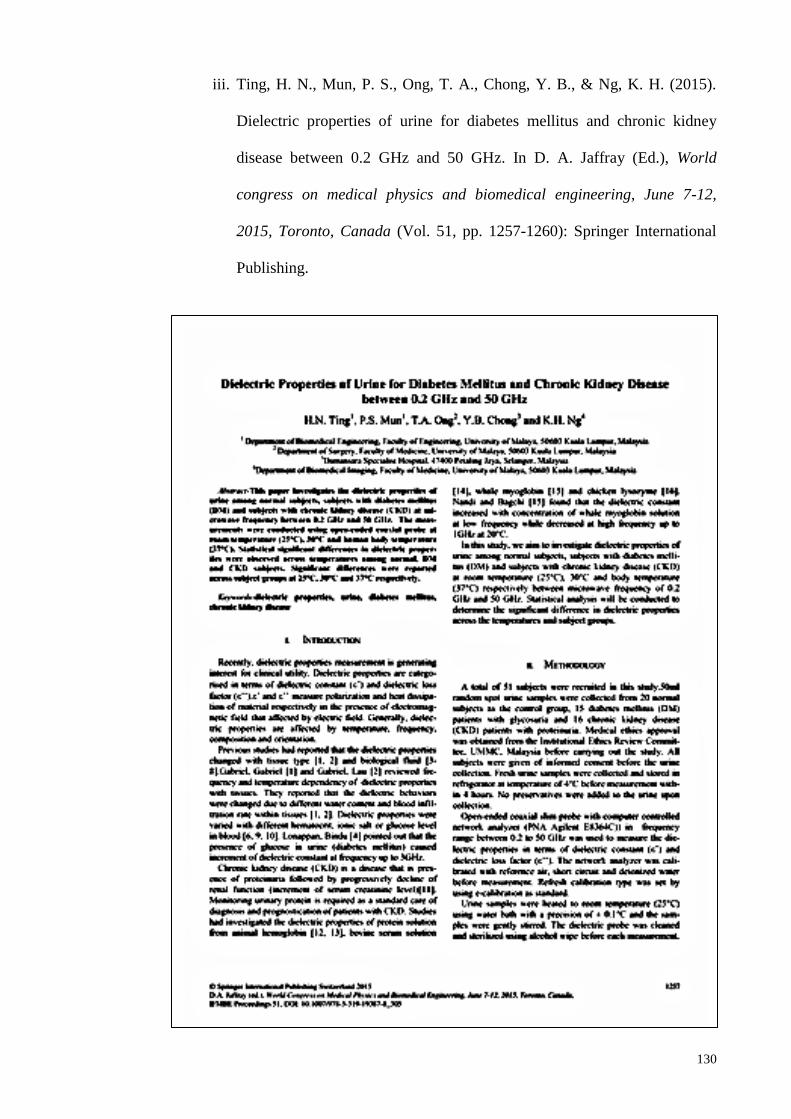
130

iii. Ting, H. N., Mun, P. S., Ong, T. A., Chong, Y. B., & Ng, K. H. (2015).

Dielectric properties of urine for diabetes mellitus and chronic kidney

disease between 0.2 GHz and 50 GHz. In D. A. Jaffray (Ed.), World

congress on medical physics and biomedical engineering, June 7-12,

2015, Toronto, Canada (Vol. 51, pp. 1257-1260): Springer International

Publishing.

131

iv. Mun, P. S., Ting, H. N., Ong, T. A., & Chong, Y. B. (2015) Urinary

dielectric properties classification for chronic kidney disease between 1

GHz and 50 GHz. Paper presented at the International Conference on Life

Science and Biological Engineering, Tokyo, Japan.

132

APPENDIX A: COMPLEX CURVE FITTING PROGRAM

% Complex curve fitting program to find parameter values of a single-pole Debye

model

% Function providing the best fit to measured dielectric properties data.

function score = opt3(P1)

P1=P1';

tic

%

% INPUT DATA

%

j=1i;

f = [10e9 20e9 30e9 40e9 50e9];

Em = [65.16-j*23.29 48.16-j*33.56 34.35-j*34.27 25.34-j*31.65 19.32-j*28.32];

%

% SET A FEW CONSTANTS

%

Eo = 8.854191e-12;

alpha = 0;

Max_score = 100;

%

% MAIN CALCULATION

%

% Sets range of search space and resolution

%

% a = [10:0.1:90]; % static permittivity

% b = [1:0.1:10]; % infinite permittivity

133

% c = [5e9:1e8:30e9]; % relaxation frequency

% d = [0:0.01:2.0]; % static conductivity

% e = [0:0.01:1.0]; % alpha parameter

%LB = [10;1;5e9;0;0];UB = [90;10;30e9;2;1];

a = P1(1,1);

b = P1(2,1);

c = P1(3,1);

d = P1(4,1);

%

% Calculates successive trial values

%

Ez = a;

Ei = b;

fc = c;

conds = d;

tau = (2*pi*fc)^-1;

w = 2*pi.*f;

Ec = Ei + ((Ez-Ei)./(1+(j.*(w.*tau).^(1-alpha)))) - (j*conds./(w.*Eo));

%

% Calculates rms percentage error over all data points

delta_Ere = (real(Ec)-real(Em)).*100./real(Em);

delta_Eim = (imag(Ec)-imag(Em)).*100./imag(Em);

score = sqrt((sum(delta_Ere.^2)+sum(delta_Eim.^2))/(2*length(Ec)));

%

% Keeps the lowest score and best solution

134

%

if score < Max_score

Max_score = score;

Best_score = score;

Best_Ec=Ec;

Best_Ei=Ei;

Best_Ez=Ez;

Best_fc=fc;

Best_conds=conds;

else

end

toc

135

APPENDIX B: GENETIC ALGORITHM

% To compute function score of complex curve-fitting program with iterations.

% Genetic algorithm (GA) performs direct search optimized parameters with best

fitness

fval1 = 100;

for i=1:15

options=

gaoptimset('Generations',200,'Display','iter','CrossoverFraction',0.5,'StallTimeLimit',Inf,

'PopulationSize',1500);

LB = [10;1;5e9;0];

UB = [90;10;30e9;2];

[x,fval] = ga(@opt3,4,[],[],[],[],LB,UB,[],options);

num2str([fval x])

if fval<fval1

fval1=fval;

x1 = x;

end

end

x1

fval1

136

APPENDIX C: SVM CLASSIFICATION PROGRAM

% To classify urinary dielectric properties of subject groups using three fold-cross

validation by using RBF kernel

CM = zeros(3,3);

data = xlsread('raw data (svm 1).xls');

a = data(2:end,1:end);

xdata = a(:,2:end);

group=a(:,1);

indices = crossvalind('Kfold',group,3);

cp = classperf(group);

for i = 1:3

test = (indices == i); train = ~test;

class = classify(xdata(test,:),xdata(train,:),group(train,:));

classperf(cp,class,test)

trainingsample=xdata(train,:);

traininglabel=group(train,1);

testingsample=xdata(test,:);

testinglabel=group(test,1);

model = svmtrain(traininglabel,trainingsample,'-s 0 -c 8 -t 2 -g 0.5 -e 0.1');

[predicted_label, accuracy, decision_values] = svmpredict(testinglabel,testingsample,

model);

for ii=1:size(predicted_label,1)

CM(testinglabel(ii,1),predicted_label(ii,1))=CM(testinglabel(ii,1),predicted_label(ii,1))

+1;

end

end

measurement and classification of urinary … · diagnosis and monitoring of diabetes and chronic...

Documents