mean loads on vaulted canopy roofs: tests in … · mean loads on vaulted canopy roofs: tests in...
TRANSCRIPT

Mean loads on vaulted canopy roofs: tests in boundary layer wind tunnel
M.B. Natalini1, C. Morel
2, B. Natalini
3, O. Canavesio
4
1Prof. of Civil Eng., Univ. Nac. del Nordeste, Resistencia, Argentina, [email protected]
2Assistant Prof. of Civil Eng., Univ. Nac. del Nordeste, Rcia., Argentina, [email protected]
3Prof. of Mechanical Eng., CONICET-UNNE, Resistencia, Argentina, [email protected]
4Assistant Prof. of Civil Eng., Univ. Nac. del Nordeste, Rcia., Argentina, [email protected]
ABSTRACT
The vaulted canopy roof (VCR) is a widespread structure in vast areas of South-America,
especially in parts of Argentina, Brazil and Paraguay. Information about the aerodynamics of
VCRs however, is scarce in the open literature. This paper presents the results of mean wind
loads coefficients on VCRs obtained in boundary layer tunnel tests, which constitute a firm base
to assess wind loads on the structure.
INTRODUCTION
The vaulted canopy roof (VCR) is a widespread structure in vast areas of South-America,
especially in parts of Argentina, Brazil and Paraguay where the climate is warm. They can be
seen across both urban and rural areas, in a wide variety of uses. For instance, a common
landmark in the north-east of Argentina, is a carpenter’s workshop sheltered by a VCR.
Information available in the specialized literature about the aerodynamic behavior of VCRs is
scarce. Cook [1] summarized this situation when he wrote: “There are only a small amounts of
data for curved canopies and these are all early data obtained in smooth uniform flow. For
example Irminger and Nokkentved included a barrel vault canopy with a rise of r = W/4 in their
studies published in 1936, and Blessmann included domed canopies with rises W/4 y W/8 in his
1971 studies. The validity of the loading coefficient is open to question in the light of current
techniques, however the general loading characteristics may be still be useful.”. This situation is
also reflected in the codes of practice. The authors of this work found only two codes that
provide loads coefficient values for VCRs: the French code NV 65 [2] and the Argentinean code
CIRSOC 102 [3]; the former having been superseded by the Eurocode and the later being
superseded by a new version that will be shortly come into effect [4]. Both codes suggest using
the same mean pressure coefficients of planar canopy roofs while keeping the same relation
rise/span. Marighetti et al. [5] though, showed that this approximation is incorrect in their
presentation of wind tunnel results of mean pressure distributions on VCRs which they compared
with the those corresponding to a planar canopy roof with similar dimensions. Fig. 1 reproduces
two figures from their work, corresponding to incident wind angles of 45º and 90º relative to the
ridge. It can be seen that the contour plots have different patterns as well as different values,
which is not surprising taking into account that it is hardly possible that the flow over a surface
with sharp edges would be similar to the flow over a relatively smooth curved surface.
Reports on boundary layer wind tunnel tests related to these structures have also not been found
in the literature, apart from those of Natalini et al. [6, 7, 8]. Regarding computational modelling
the situation is similar, though there have been recently some promising results reported by
Balbastro et al. [9, 10, 11].

Curved Planar Curved Planar
Fig. 1: Contour plots of mean pressure coefficients over curved and planar canopy roofs (after Marighetti et
al. [5]).
Considering the lack of reliable data sources for state-of-art wind engineering and that the
structural designer needs design aerodynamic coefficients, the subject was the object of a wind-
tunnel-based studio in the Laboratorio de Aerodinámica de la Facultad de Ingeniería de la
Universidad Nacional del Nordeste (UNNE), Argentina.
This paper presents results of mean wind loads coefficients on VCRs obtained in boundary layer
tunnel tests. The first problem approached was the selection of the most suitable technique for
modeling pressures on curved surfaces. Once the modeling conditions were established, local
and global wind load coefficients were determined on models of six VCRs of different geometry
using wind simulation.
WIND TUNNEL MODELING TECHNIQUES
The study of these structures through wind tunnel tests presents difficulties inherent to both free-
standing canopies and bodies with curved surfaces, for which it was necessary to develop
specific modeling techniques. The first problem approached was the selection of the most
suitable technique for modeling pressures on curved surfaces. The issue of modelling wind loads
on VCRs was approached by Natalini et al. [6], who based in previous work of Ribeiro [12],
Cheung and Melbourne [13], Batham [14], Blackbourn and Melbourne [15], Blessmann and
Loredo Souza [16] and Blessmann [17], tested three 1:75 scale models of similar geometry but
different roughness over the roof. As a result, sand of appropriate size was added to the upper
side of the roof of the models.
On the other hand, Natalini et al. [18] reported a study on the modelling of mean pressures on
planar canopy roofs. The paper presented wind tunnel results of tests on scale models of the full-
scale Dutch barn tested by Robertson et al. [19] at Silsoe, UK. The comparison between both full
and reduced scale barns showed that severe distortions can appear which are linked to scale
effects if the size of the model is below a certain level. In the case of the UNNE tunnel such
distortion did not manifest when using a 1:75 scale model [20]. Based in these experiences the
scale 1:75 was adopted for all the models used in the present study.

EXPERIMENTAL ARRANGEMENT
MODELS
The geometry and size of the six models that were tested were adopted on account of the range
of dimensions of the VCRs more frequently found in the north-east of Argentina, and the size of
the models of enclosed buildings appearing in the literature. Fig. 2 and Table 1 summarize the
geometry of the models.
Fig. 2: Geometry of the models.
Table 1: Dimensions of the models.
The rise, f, and the span, b, was kept similar in all models. Basically, two kinds of models were
built, the deep models (A, B and C) and the short models (D, E and F), which allowed the
assessment of the influence of the depth. By varying the height of the eves, h, (2, 4 and 6 cm),
the six models were produced. It is clear that models C and F, with a h dimension that
corresponds to 1.5 m at full-scale, do not represent any real situation. They have been included in
the tests in order to observe the trend that pressures follow when varying the height of the eves.
Wind load coefficients were measured under wind blowing at angles of 60º, 75º and 90º relative
to the ridge line since, as demonstrated by Natalini et al. [8], these directions produce the most
severe loads.
The roof of the models was made with a 2 mm thick aluminium plate, and the columns with a 2.5
mm diameter steel rod (except one column, the farthest one from the area where taps were
placed, which had a square cross section of 10 × 10 mm). As the models have two axes of
Absolute dimensions Relative dimensions
Mo
del
a
[cm]
b
[cm] h [cm]
f
[cm] b/a h/b f/b f/h
r
[cm] α Re × 10
5
A 60 15 6 3 0.25 0.40 0.20 0.5 10.88 43º58’ 2.09
B 60 15 4 3 0.25 0.27 0.20 0.75 10.88 43º58’ 1.96
C 60 15 2 3 0.25 0.133 0.20 1.50 10.88 43º58’ 1.68
D 30 15 6 3 0.50 0.40 0.20 0.50 10.88 43º58’ 2.09
E 30 15 4 3 0.50 0.27 0.20 0.75 10.88 43º58’ 1.96
F 30 15 2 3 0.50 0.133 0.20 1.50 10.88 43º58’ 1.68
b
h
f
r α
a

symmetry, only a quarter of the models' roofs had pressure taps in place, in this way reducing the
number of tubes needed. In addition, all the tubes were led towards the farthest column, through
which they reached the floor. In this way, the scale distortion in both columns and roof thickness
and the possible interference of the tubes upon the measurements were minimized.
In order to obtain a flow in transcritical conditions, sand was added to the upper side of the roof
of the models, being the relative roughness, dk / , equal to 3.30 × 10³.
WIND SIMULATION
The wind tunnel tests were undertaken in the “Jacek P. Gorecki” wind tunnel at the Universidad
Nacional del Nordeste. This is an open return wind tunnel with a working section of 22.4 m in
length × 2.4 m in width × 1.8 m in height and a maximum flow velocity of 25 m/s when the
working section is empty. Further details are given by Wittwer and Möller [21].
All the models were tested under a wind simulation corresponding to a suburban area. The
simulation hardware consisted of two modified Irwin’s spires [22] and 17.1 m of surface
roughness fetch downstream from the spires. In this way, a part-depth boundary layer simulation
of neutrally stable atmosphere was obtained. Mean velocities, when fitted to a potential law, give
an exponent of 0.24. The length scale factor determined according to Cook’s procedure [23] was
about 150. The local turbulence intensity at the level of the roof is 0.25. De Bortoli et al. [24]
gave further details of this simulation, including size, geometry and arrangement of the hardware
and design criteria.
PRESSURE MEASUREMENT SYSTEM
Pressures were measured using a differential pressure electronic transducer Micro Switch
Honeywell 163 PC. A sequential switch Scanivalve 48 D9-1/2, which was driven by means of a
CTLR2 / S2-S6 solenoid controller connected the roof pressure taps to the transducer through
PVC tubes of 1.5 mm in internal diameter and 400 mm in length. No resonance problems were
detected for tubes of that length (the gain factor being around one) therefore restrictors of section
were not used for filtering. The DC transducer output was read with a Keithley 2000 digital
multimeter. The integration time operation rate of the A/D converter was set to produce mean
values over 55 seconds.
Simultaneously to the pressure measurements being taken on the roof, the reference dynamic
pressure, qref, was measured at the eaves height with a Pitot-Prandtl tube connected to a Van
Essen 2500 Betz differential micromanometer of 1 Pa resolution. The probe stayed beside the
model at a distance of about 70 cm to avoid mutual interference. The reference static pressure
was obtained from the static pressure tap of the same Pitot-Prandlt tube.
RESULTS
PRESSURE COEFFICIENTS
The net pressure coefficient, pc , was obtained by subtracting the internal pressure coefficient,
pic , from the external pressure coefficient, pec . The two last coefficients are the rate between
the pressure on the tap, p, which can be either an external or internal pressure, and qref , which is
the reference dynamic pressure measured at the reference height. Here, the tap pressures are
relatives to the static reference pressure, refp , which is obtained from the static tap of the same
Pitot-Prandtl tube used to measure qref. Following the usual convention, negative values of both

pec and pic indicate actions directed out from the surface (suctions). Accordingly, positive
values of pc indicate actions directed into the building. In this work, the most positive and
negative values of a set of pressure coefficient will be referred as the maximum and minimum
values of that set.
The whole set of contour plots were given by Natalini [25], including figures of internal, external
and net pressure coefficients. When comparing pressures on deep and short models, at first
glance they show more similarities than disparities. However, two differences can be noted,
though they are restricted to the central area of the roofs. On the one hand, external pressures are
slightly higher near the upwind eave of the deep models and the zero pressure coefficient line is
shifted towards leeward; on the other hand, internal negative pressures are lower (that is bigger
in absolute value) near the ridge of the deep models.
The second difference can be better appreciated in figures 6 to 8, which show the profiles of the
pressure coefficient distribution on a cross section in the middle of the roof (section II). In
contrast, figures 3 to 5, which show the pressures on a cross section located 5 mm inwards the
upwind edge (Section I), present virtually the same figures for both models.
60º Section I. Model D
1
1.5
-2
-0.5
-1
-1.5
0.5
0
1.5
60º Section I. Model A
1
0.5
0
-0.5
-1
-1.5
-2
External pressure coefficient
Internal pressure coefficient
Net pressure coefficient
Fig. 3: External, internal and net pressure coefficients profiles. θ=60º. Upwind edge.
75º Section I. Model A
-1.5
-1
-0.5
0
0.5
1.5
1
75º Section I. Model D
1
1.5
0.5
0
-0.5
-1.5
-1
Fig. 4: External, internal and net pressure coefficients profiles. θ θ θ θ = 75º. Upwind edge.

90º Section I. Model A
-1
-0.5
0
0.5
1
90º Section I. Model D
1
1.5
0.5
0
-0.5
-1
Fig. 5: External, internal and net pressure coefficients profiles. θθθθ = 90º. Upwind edge.
60º Section II. Model A
1
0.5
0
-0.5
-1
1.5
60º Section II. Model D
1
1.5
0.5
0
-0.5
-1
Fig. 6: External, internal and net pressure coefficients profiles. θ=60º. Central section.
75º Section II. Model A
1.5
1
0.5
0
-0.5
-1
75º Section II. Model D
1
1.5
0.5
0
-0.5
-1
Fig. 7: External, internal and net pressure coefficients profiles. θ = 75º. Central section.
90º Section II. Model A
1
0.5
0
-0.5
-1
90º Section II. Model D
1
1.5
0.5
0
-0.5
-1
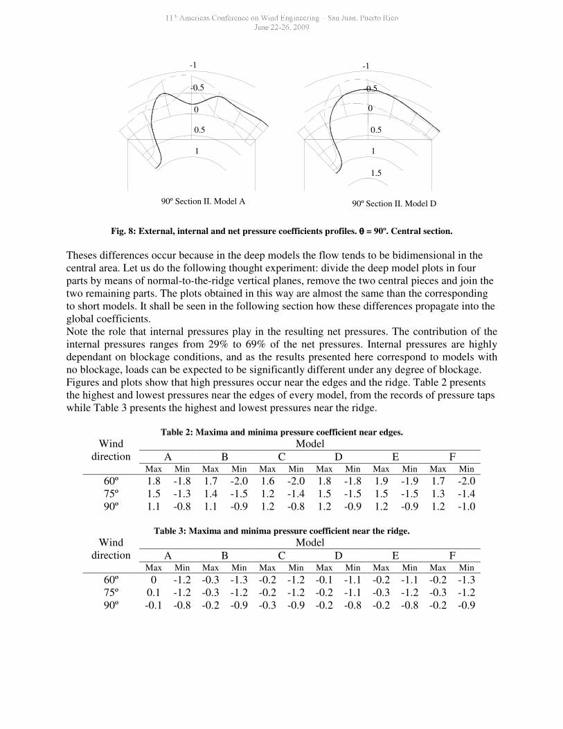
Fig. 8: External, internal and net pressure coefficients profiles. θ θ θ θ = 90º. Central section.
Theses differences occur because in the deep models the flow tends to be bidimensional in the
central area. Let us do the following thought experiment: divide the deep model plots in four
parts by means of normal-to-the-ridge vertical planes, remove the two central pieces and join the
two remaining parts. The plots obtained in this way are almost the same than the corresponding
to short models. It shall be seen in the following section how these differences propagate into the
global coefficients.
Note the role that internal pressures play in the resulting net pressures. The contribution of the
internal pressures ranges from 29% to 69% of the net pressures. Internal pressures are highly
dependant on blockage conditions, and as the results presented here correspond to models with
no blockage, loads can be expected to be significantly different under any degree of blockage.
Figures and plots show that high pressures occur near the edges and the ridge. Table 2 presents
the highest and lowest pressures near the edges of every model, from the records of pressure taps
while Table 3 presents the highest and lowest pressures near the ridge.
Table 2: Maxima and minima pressure coefficient near edges.
Model
A B C D E F
Wind
direction Max Min Max Min Max Min Max Min Max Min Max Min
60º 1.8 -1.8 1.7 -2.0 1.6 -2.0 1.8 -1.8 1.9 -1.9 1.7 -2.0
75º 1.5 -1.3 1.4 -1.5 1.2 -1.4 1.5 -1.5 1.5 -1.5 1.3 -1.4
90º 1.1 -0.8 1.1 -0.9 1.2 -0.8 1.2 -0.9 1.2 -0.9 1.2 -1.0
Table 3: Maxima and minima pressure coefficient near the ridge.
Model
A B C D E F
Wind
direction Max Min Max Min Max Min Max Min Max Min Max Min
60º 0 -1.2 -0.3 -1.3 -0.2 -1.2 -0.1 -1.1 -0.2 -1.1 -0.2 -1.3
75º 0.1 -1.2 -0.3 -1.2 -0.2 -1.2 -0.2 -1.1 -0.3 -1.2 -0.3 -1.2
90º -0.1 -0.8 -0.2 -0.9 -0.3 -0.9 -0.2 -0.8 -0.2 -0.8 -0.2 -0.9

FORCE COEFFICIENTS
The roof of the models were divided into four zones as shown in figure 9. Force coefficients
were determined by integrating the pressures on the four areas and on the whole roof.
43
yx
x
21
z
y
Reference area for global
horizontal actionson sections 1 and 3
Reference area
for global vertical
actions on sector 3
A = A
A =Y
Z Z
3
1 3
Fig. 9: Reference areas.
As force coefficients are associated with directions, a convention on the reference axes must be
formulated. The conventional axes most commonly used in aerodynamics are wind axes and
body axes. In this work, body axes are used, as displayed in figure 9. The force coefficients are
then defined as
i
ii
yref
yy
Aq
FC = i = 1,2,3,4 (1)
i
ii
zref
zz
Aq
FC = i = 1,2,3,4 (2)
yref
yy
Aq
FC = (3)
zref
zz
Aq
FC = (4)
Where iyC is the partial force coefficient on zone “i” in y-direction (horizontal), izC is the
partial force coefficient on zone “i” in z-direction (vertical), iyF is the force on zone “i” in y-

direction, izF is the force on zone “i” in z-direction, iyA = f2
a is the vertical reference area for
zone “i”, izA = ba
2 is the horizontal reference area for zone “i”, yC is the total force coefficient
in y-direction, zC is the total force coefficient in z-direction, yF is the force on the whole roof in
y-direction, zF is the force on the whole roof in z-direction, yA = a.f is the total vertical
reference area and zA = a.b is the total horizontal reference area.
The reference dynamic pressure, qref, was measured at the eave eight, as described before.
Table 4 shows the force coefficients acting on every zone (partial coefficients) and the overall
roof (total coefficients). The force coefficients are positive when the action is directed in the
positive direction of the corresponding reference axis (fig. 9).
Table 4: Force coefficients.
h/b = 0.4
Parcial Total Parcial Total θ º
1yC 2yC
3yC 4yC yC
1zC
2zC 3zC
4zC zC
60 0.31 0.43 0.65 0.33 0.86 -0.03 -0.02 0.73 0.36 0.26
75 0.43 0.50 0.54 0.35 0.91 -0.08 -0.10 0.59 0.39 020
A
90 0.35 0.35 0.45 0.45 0.80 -0.01 -0.01 0.50 0.50 0.26
h/b = 0.27
60 0. 22 0.32 0.71 0.37 0.81 0.09 0.08 0.81 0.44 0.36
75 0.32 0.39 0.64 0.47 0.91 0.05 -0.02 0.73 0.55 0.34 B
90 0.40 0.40 0.52 0.52 0.92 0.00 0.00 0.60 0.60 0.30
h/b = 0.133
60 0.34 0.36 0.56 0.36 0.81 0.00 0.02 0.66 0.45 0.28
75 0.36 0.38 0.58 0.44 0.88 0.02 0.03 0.68 0.54 0.32 C
90 0.35 0.35 0.50 0.50 0.85 0.06 0.06 0.62 0.62 0.34
h/b = 0.4
60 0.36 0.51 0.78 0.31 0.98 -0.08 -0.04 0.89 0.35 0.28
75 0.40 0.53 0.71 0.32 0.98 -0.07 -0.09 0.79 0.37 0.25 D
90 0.51 0.51 0.47 0.47 0.98 -0.12 -0.12 0.52 0.52 0.20
h/b = 0.27
60 0.34 0.62 0.78 0.32 1.03 -0.07 -0.13 0.89 0.36 0.26
75 0.39 0.58 0.74 0.35 1.03 -0.04 -0.13 0.80 0.40 0.26 E
90 0.49 0.49 0.50 0.50 0.99 -0.10 -0.10 0.55 0.55 0.23
h/b = 0.133
60 0.31 0.55 0.85 0.35 1.03 0.01 -0.08 0.96 0.43 0.33
75 0.38 0.48 0.75 0.43 1.02 0.01 0.02 0.85 0.52 0.34 F
90 0.49 0.49 0.55 0.55 1.04 -0.08 -0.08 0.64 0.64 0.29

If the yC coefficients of short and deep models are compared, it can be observed that in general
terms the ones corresponding to short models are about 10% higher for any h/b relationship. This
difference becomes even more evident between models B and E, where the disparity is 21%.
It is interesting to view figures 10 and 11, which have been built with values extracted from
Table 4. Figure 10 summarizes the variation of the total force coefficient in the y-direction for all
models in regard to θ and h/b. The coefficients of the A, B and C models are at the left of the
figure, clearly separated from those of the D, E and F models. The yC on the short models are
higher than the corresponding ones of the deep models for every value of θ and h/b, and in this
case they are not sensitive to θ and h/b, the values range between 0.98 and 1.04. Deep models
proved to be more sensitive, being the most severe case when the wind direction is 75º.
In figure 11 the variation of the total force coefficient in the z-direction is shown. In this
example, even though the curves follow the same trend but are inverted, they are not as clearly
split up as the yC values in fig. 10. For h/b = 0.27 the values of zC are higher on deep models,
but in the other two cases they are merged with the ones of the short models. Note that for θ =
90º the variation is practically linear with h/b.
In the previous section, it was pointed out that in the central area of the deep models roofs,
external pressures near the upwind eave are smaller than those of short models. This causes the
net pressure on that area to be smaller on deep roofs, which contributes to both decreased yC
and increased zC in regard to the short models. On the other hand, as internal negative pressures
are lower (that is bigger in absolute value) near the ridge of the deep models, they contribute to
decrease both yC and zC . As both effects add up to influence on yC , they explain the clear
separation in figure 10, and as they have an opposite influence on zC , they also explain the fact
that zC figures are a bit entangled in figure 11.
0,10
0,15
0,20
0,25
0,30
0,35
0,40
0,45
0,78 0,83 0,88 0,93 0,98 1,03Cy
h/b
60 deep 75 deep 90 deep 60 short 75 short 90 short
Fig. 10: Variation of the total force coefficient in the y-direction.

0,10
0,15
0,20
0,25
0,30
0,35
0,40
0,45
0,19 0,21 0,23 0,25 0,27 0,29 0,31 0,33 0,35 0,37Cz
h/b
60 short 75 short 90 short 60 deep 75 deep 90 deep
Fig. 11: Variation of the total force coefficient in the z-direction.
CONCLUSIONS
Marighetti et al. [5] demonstrated that pressures on VCR are different from pressures on planar
canopy roofs, for which reason it is a mistake to estimate the loads on VCRs by approximating
them with those on planar canopy roofs, as advised in some codes of practice. In this paper,
results of mean wind loads coefficients on vaulted canopy roofs obtained in boundary layer
tunnel tests have been presented. These results constitute a firm base to assess wind loads on
VCRs, though it must be noted that tests have been limited to models with a relation rise/span f/b
= 0.20, therefore estimating loads for others relation f/b is not straightforward.
Positive and negative pressures reach important values near the edges and the ridge. Tables 2 and
3 show the maxima and minima pressure coefficients in those zones of all models and for all the
wind directions tested; they can be used to verify cladding and structural parts. Global
coefficients given in Table 4 establish the total force acting on the structure, which is necessary
information for the design of the immediately supporting structure.
Mean aerodynamic coefficients on VCRs are influenced by size relations. They vary with the
column height and the relation span/depth. The maxima mean net pressure coefficients are higher
on the short models, while the minima mean net pressure coefficients occur on deep models. The
absolute value of pressure coefficients show a general trend to increase as the column height
decreases. As for the global coefficients, yC values are higher on short roofs and zC values are,
mostly but not always, higher on deep roofs.
ACKNOWLEDGEMENTS
The authors wish to acknowledge the help of Jose A. Iturri in making the models and preparing
the experimental set-up. The present work is part of an area of research supported by the
Facultad de Ingeniería de la Universidad Nacional del Nordeste, Argentina.
REFERENCES
[1] N.J. Cook, The designer's guide to wind loading of building structures, part 2: static structures,
Building Research Establishment Report, London, 1990.
[2] NV 65 Règles définisant les effets de la neige et du vent sur les constructions et annexes. Societé de
Diffusion des Techniques du Bâtiment et des Travaux Publics, France, 1970.
[3] CIRSOC 102: Acción del viento sobre las construcciones. Instituto Nacional de Tecnología
Industrial, Buenos Aires, 1983.
[4] CIRSOC 102: Reglamento Argentino de acción del viento sobre las construccione. Instituto Nacional
de Tecnología Industrial, Buenos Aires, 2005.
[5] J.O. Marighetti, O. Canavesio, B. Natalini, M.B. Natalini, Comparación entre coeficientes de presión
media en cubiertas aisladas planas y curvas, Memorias de las XVII Jornadas Argentina de Ingeniería
Estructural, Rosario, Argentina, 2002.
[6] M.B. Natalini, O. Canavesio, B. Natalini,M.J. Paluch, Wind tunnel modelling of mean pressures on
curved canopy roofs, Proceeding of the Americas Conference on Wind Engineering, Clemson, USA,
2001.
[7] M.B. Natalini,O. Canavesio,B. Natalini,M.J. Paluch, Pressure distribution on curved canopy roof,
Proceedings of The Second International Symposium on Advances in Wind and Structures, Pusan, Korea
2002.
[8] M.B. Natalini,C, Morel, B., Natalin,. Mean wind loads on vaulted canopy roofs under different wind
directions, Revista Sul-Americana de Engenharia Estrutural. 2 (2005) 29-40.
[9] G. Balbastro, V. Sonzogni, G. Franck, Simulación numérica del viento sobre una cubierta abovedada,
Mecánica Computacional. 24 (2005) 1261-1278.
[10] G. Balbastro,V. Sonzogni, Coeficientes de presión en cubiertas abovedadas aisladas, Anales de XIX
Jornadas Argentinas de Ingeniería Estructural, Mar del Plata, Argentina, 2006.
[11] G. Balbastro,V. Sonzogni, Simulación de un ensayo en túnel de viento aplicando CFD, Mecánica
Computacional, 26 (2007) 3779-3787.
[12] J.L.D. Ribeiro, Effects of surface roughness on the two-dimensional flow past circular cylinders,
Journal of Wind Engineering and Industrial Aerodynamics. 37( 1991) 299-309.
[13] J.C.K. Cheung, W.H. Melbourne, Turbulence effects on some aerodynamics parameters of a circular
cylinder at supercritical numbers, Journal of Wind Engineering and Industrial Aerodynamics. 14 (1983)
399-410.
[14] J.P. Batham, Wind tunnel test on scale models of a large power station chimneys, Journal of Wind
Engineering and Industrial Aerodynamics. 18 (1985) 87-91.
[15] H.M. Blackburn,W.H. Melbourne, The Effect of free-stream turbulence on sectional lift forces on a
circular cylinder, Journal of Fluid Mechanics. 306 (1996) 267-292.
[16] J. Blessmann, J., A.M. Loredo Souza, Açao do vento em coberturas curvas, Caderno Técnico CT-94,
Universidade Federal do Rio Grande do Sul, Brasil, 1998.
[17] J. Blessmann, Wind load on isolated and adjacent industrial pavilion curved roof. In: Wind Effects
on Buildings and Structures (Gramado, Brasil, 1998), Balkema, Rotterdam,1998. pp. 137-171.

[18] B. Natalini, O. Marighetti, M.B. Natalini, Wind tunnel modelling of mean pressures on planar
canopy roof, Journal of Wind Engineering and Industrial Aerodynamics. 90 (2002) 427-439.
[19] A.P Robertson, R.P. Hoxey, P. Moran, A full scale study of wind loads on agricultural ridged
canopy roof structures and proposal for design, Journal of Wind Engineering and Industrial
Aerodynamics. 21 (1985) 167-205.
[20] B. Natalini, O, Marighetti, M.B. Natalini,Wind tunnel test of planar canopy roof model. Memorias
de las XXIX Jornadas Sudamericanas de Ingeniería Estructural, Punta del Este, Uruguay, 2000.
[21] A.R. Wittwer, S.V. Möller, Characteristics of the low-speed wind tunnel of the UNNE, Journal of
Wind Engineering and Industrial Aerodynamics. 84 (2000) 307-320.
[22] H.P.A.H. Irwin, The design of spires for wind simulation, Journal of Wind Engineering and
Industrial Aerodynamics. 7 (1981) 361-366.
[23] N.J Cook,. Determination of the model scale factor in wind-tunnel simulations of the adiabatic
atmospheric boundary layer, Journal of Wind Engineering and Industrial Aerodynamics. 2 (1977/1978)
311-321.
[24] M.E. De Bortoli, B. Natalini, B., M.J. Paluch, M.B. Natalini, Part-depth wind tunnel simulations]of
the atmospheric boundary layer, Journal of Wind Engineering and Industrial Aerodynamics. 90 (2002)
281-291.
[25] M.B. Natalini, Acción del viento sobre cubiertas curvas aisladas, Tesis de Doctorado, Universidad
Nacional del Nordeste, Argentina (in Spanish), 2005.