mean-field theory and computation of electrostatics with...
TRANSCRIPT

Mean-Field Theory and Computation of Electrostaticswith Ionic Concentration Dependent Dielectrics
Bo Li∗ Jiayi Wen † Shenggao Zhou ‡
January 1, 2015
Abstract
We construct a mean-field variational model to study how the dependence of di-electric coefficient (i.e., relative permittivity) on local ionic concentrations affects theelectrostatic interaction in an ionic solution near a charged surface. The electrostaticfree-energy functional of ionic concentrations, which is the key object in our model,consists mainly of the electrostatic potential energy and the ionic ideal-gas entropy.The electrostatic potential is determined by Poisson’s equation in which the dielec-tric coefficient depends on the sum of concentrations of individual ionic species. Thisdependence is assumed to be qualitatively the same as that on the salt concentrationfor which experimental data are available and analytical forms can be obtained by thedata fitting. We derive the first and second variations of the free-energy functional,obtain the generalized Boltzmann distributions, and show that the free-energy func-tional is in general nonconvex. To validate our mathematical analysis, we numericallyminimize our electrostatic free-energy functional for a radially symmetric charged sys-tem. Our extensive computations reveal several features that are significantly differentfrom a system modeled with a dielectric coefficient independent of ionic concentration.These include the non-monotonicity of ionic concentrations, the ionic depletion near acharged surface that has been previously predicted by a one-dimensional model, andthe enhancement of such depletion due to the increase of surface charges or bulk ionicconcentrations.
Key words and phrases: Electrostatic interactions, concentration-dependent di-electrics, mean-field models, Poisson–Boltzmann theory, generalized Boltzmann dis-tributions, nonconvex free-energy functional, variational analysis, numerical compu-tation.
∗Department of Mathematics and Center for Theoretical Biological Physics, University of California, SanDiego, 9500 Gilman Drive, Mail code: 0112, La Jolla, CA 92093-0112, USA. Email: [email protected].†Department of Mathematics and Center for Theoretical Biological Physics, University of California,
San Diego, 9500 Gilman Drive, Mail code: 0112, La Jolla, CA 92093-0112, USA. E-mail: [email protected].‡Department of Mathematics and Center for Theoretical Biological Physics, University of California, San
Diego, 9500 Gilman Drive, Mail code: 0112, La Jolla, CA 92093-0112, USA. Email: [email protected].
1

1 Introduction
Electrostatic interactions among charged solutes, mobile ions, and polarized solvent playan important role in the stability and dynamics of biological molecules in aqueous solution[4,13,16,28,29,42–44,53,54]. Poisson’s equation and Poisson–Boltzmann (PB) equations areefficient mathematical descriptions of such interactions [3,11,13,14,19,21,24,25,36,45,53].A basic hypothesis in such descriptions is that an underlying charged molecular systemcan be treated as a dielectric medium characterized by its dielectric coefficient that canvary spatially. Under normal conditions, the dielectric coefficient for water is close to 80,while that for proteins can be as low as 1 – 4 [26,27]. Experiment and molecular dynamics(MD) simulations have indicated that the dielectric coefficient can depend on the local ionicconcentrations [9,10,17,26,27,31,33,40,47,50–52,57,58]. In this work, we use a mean-fieldvariational approach to study how such dependence affects the equilibrium properties ofelectrostatic interactions in an ionic solution.
0 1 2 3 4 5 6 7 810
20
30
40
50
60
70
80
Concentration (M)
Die
lectr
ic C
oeffic
ient of N
aC
l
Fitted Curve
Experimental Data 1
Experimental Data 2
Figure 1.1: The dielectric coefficient for NaCl solution. The experimental data 1 and 2are taken from [27] and [40], respectively. The fitted form is ε(c) = 70e−0.22c + 10. Themaximum relative error at data points is 2%.
Consider an ionic solution near a charged surface. Assume there are M ionic species inthe solution. (Typically 1 ≤ M ≤ 4.) Denote by ci = ci(x) the local ionic concentrationof the ith species at a spatial point x. Our key modeling assumption is that the dielectriccoefficient ε depends on the sum of local ionic concentrations of all individual ionic (eithercationic or anionic) species: ε = ε(c(x)), where c =
∑Mi=1 ci. This dependence is qualita-
tively the same as that on the salt concentration. The latter can be constructed by fittingexperimental or MD simulations data. Figure 1.1 shows the dependence of the dielectriccoefficient on the concentration of NaCl [27, 40] and the fitted analytic form of such de-pendence. In general, we assume that the function ε = ε(c) is monotonically decreasing,convex, and is bounded below by a positive constant. Examples of such a function ε = ε(c)
2

are
ε(c) =α0 − α1
1 + ξ c+ α1 and ε(c) = (α0 − α1)e−ξ c + α1,
where all α0, α1, and ξ are constant parameters fitting experimental or MD simulationsdata with α0 > α1 > 0. Note that ε(0) = α0 and ε(∞) = α1. We remark that the choiceof c instead of salt concentration reflects our attempt in understanding the contributionof each individual ionic species through its concentration to the dielectric environment, asbiological properties are often ion specific (e.g., the ion selectivity in ion channels). Usingc =
∑Mi=1 ci allows us to input the concentration of each individual ionic species, and also
to determine the variation of the free energy with respect to such individual ionic species.The dielectric coefficient measures the polarizability of a material exposed to an external
electric field. Due to their asymmetric structures, water molecules form permanent dipoles.They orient randomly in the bulk due to thermal fluctuations. Such orientational polariza-tion makes the bulk water a strong dielectric medium. In the proximity of charged particlessuch as ions (cations or anions), however, water molecules are attracted by the charges,forming a hydration shell. These dipolar water molecules in the shell are aligned to thelocal electric field. Such saturation of local orientational polarizability leads to a weakerdielectric response of water near charges to the external electric field. Consequently, thedielectric coefficient in a region of high ionic concentrations is expected to be smaller thanthat in a region of lower ionic concentrations [7, 15, 22, 27, 57]. This dielectric decrement isone of the main properties of electrostatic interactions that we study here.
+
–+
+
++
+
+
++
+
+
+
++
+
+
+
+ –
–
–
–
–
––
–
–
–
–
–
–
–
– –
Ω
ΓD
ΓN
Figure 1.2: A schematic view of an ionic solution. The solvent occupies the grey regionΩ. Small circles with plus and minus signs represent cations (positively charged ions) andanions (negatively charged ions), respectively.
We now let the ionic solution occupy a bounded domain Ω in R3 with a smooth boundary∂Ω. We assume that the boundary ∂Ω of Ω is divided into two nonempty, disjoint, andsmooth parts ΓD (D for Dirichlet) and ΓN (N for Neumann); cf. Figure 1.2. (The casethat ΓD = ∅, i.e., Γ = ΓN, can be treated similarly.) We also assume that we are given a
3

fixed charged density ρf : Ω → R, a surface charge density σ : ΓN → R, and a boundaryvalue of the electrostatic potential ψ∞ : ΓD → R. We consider minimizing the followingmean-field electrostatic free-energy functional of the ionic concentrations c = (c1, . . . , cM)[12,20,36,48,49]:
F [c] =
∫Ω
1
2ρ(c)ψ(c) dV +
∫ΓN
1
2σψ(c) dS + β−1
M∑i=1
∫Ω
ci[log(Λ3ci)− 1
]dV
−M∑i=1
µi
∫Ω
ci dV. (1.1)
Here, the first two terms together represent the electrostatic potential energy. In theseterms, ρ(c) is the total charge density, defined by
ρ(c) = ρf +M∑i=1
qici, (1.2)
where qi = Zie with Zi the valence of the ith ionic species and e the elementary charge, andψ = ψ(c) is the electrostatic potential determined as the solution to the boundary-valueproblem of Poisson’s equation [7, 30,32]
∇ · ε(c)ε0∇ψ = −ρ(c) in Ω,
ε(c)ε0∂ψ
∂n= σ on ΓN,
ψ = ψ∞ on ΓD,
(1.3)
where ε0 is the vacuum permittivity and ∂ψ/∂n denotes the normal derivative at Γ withn the exterior unit normal. The third term in (1.1) represents the ionic ideal-gas entropy,where β−1 = kBT with kB the Boltzmann constant and T the absolute temperature, logdenotes the natural logarithm, and Λ is the thermal de Broglie wavelength. The last term in(1.1), in which µi is the chemical potential for the ith ionic species, represents the chemicalpotential of the system that results from the constraint of total number of ions in eachspecies.
Our main contributions are as follows:(1) We derive the first and second variations of the electrostatic free-energy functional
(1.1). Setting the first variation to zero, we obtain the following generalized Boltzmanndistributions that relate the equilibrium concentrations c1, . . . , cM to the correspondingelectrostatic potential ψ :
ci = c∞i exp
−β[qiψ +
1
2ε′(c)ε0|∇ψ|2
], i = 1, . . . ,M, (1.4)
where c∞i is the bulk concentration of the ith ionic species that is determined by theparameters Λ and µi. Here we assume ψ∞ = 0. A more general formula is given inSubsection 2.2. This formula was obtained in [7] for a one-dimensional system and a
4

linear ε = ε(c). Note that if ε does not depend on the concentrations then ε′(c) = 0,and we recover the classical Boltzmann distributions. If ε = ε(c) is linear in c asassumed in [7,27], then ε′(c) does not depend on c and the equilibrium concentrationsare uniquely determined by the potential ψ. In the general case, where ε = ε(c) isnonlinear in c, the equilibrium concentrations are only defined implicitly by (1.4)through the potential ψ.
(2) We show by numerical calculations that there are possibly multiple values of con-centrations c = (c1, . . . , cM) that can depend on the same potential ψ through thegeneralized Boltzmann distributions. We also construct some examples to prove thatthe free-energy functional can be indeed nonconvex.
(3) We minimize numerically our electrostatic free-energy functional for a radially sym-metric system of both counterions and coions. By our extensive numerical computa-tions, we find several interesting properties of the electrostatic interactions attributedto the dependence of dielectric on ionic concentrations. These include the depletion ofions near a charged surface that has been previously described by a one-dimensionalmodel with a linear ε = ε(c) [7], the non-monotonicity of ionic concentrations nearsuch a surface, and the shift of peaks of the ionic concentration profiles due to theincrease of surface charges or bulk concentrations.
Our free-energy functional (1.1) extends those in [12, 20, 36, 49], where the dielectriccoefficient is independent of concentrations, and that in [7], where the dielectric coefficientdepends linearly on the concentrations. A nonlinear dependence of dielectric coefficienton concentrations is significant, as it can lead to the existence of multiple equilibriumconcentrations. Our numerical results show interesting phenomena, extending those foundin [5,7,22,31,34]. We notice that several authors have studied the dielectric decrement andrelated issues through the polarization of solvent molecules and ions [1, 5, 6, 22, 46].
We organize the rest of the paper as follows: In Section 2, we derive the first variationsof the free-energy functional and the generalized Boltzmann distributions. In Section 3,we derive the second variations of the free-energy functional. In Section 4, we show bynumerical calculations that the generalized Boltzmann distributions can lead to multiplevalues of concentrations. We also show by examples that the free-energy functional isin general nonconvex. In Section 5, we minimize numerically the mean-field electrostaticfree-energy functional for a radially symmetric system. Finally, in Section 6, we draw ourconclusions.
2 First Variations and Generalized Boltzmann Distri-
butions
Unless otherwise stated, we assume the following throughout the rest of the paper:(A1) The dielectric coefficient function ε ∈ C1([0,∞)). It decreases monotonically and is
convex. Moreover, there are two positive numbers εmin and εmax such that
εmin ≤ ε(c) ≤ εmax ∀c ≥ 0; (2.1)
5

(A2) The set Ω ⊂ R3 is bounded, open, and connected with a smooth boundary Γ = ∂Ω(e.g., Γ is in the class C2). The boundary ∂Ω is divided into two disjoint, nonempty,and smooth (e.g., in the class of C2) parts ΓD and ΓN;
(A3) The functions ρf : Ω → R, σ : ΓN → R, and ψ∞ : ΓD → R are all given. Moreover,ρf ∈ L∞(Ω), σ is the restriction of a W 1,∞(Ω)-function (also denoted by σ) on ΓN,and ψ∞ is the restriction of a W 2,∞(Ω)-function (also denoted by ψ∞) on ΓD.
Note that we use standard notion for Sobolev spaces [2, 18,23].We denote
H1D,0(Ω) =
φ ∈ H1(Ω) : φ = 0 on ΓD
,
H1D(Ω) =
φ ∈ H1(Ω) : φ = ψ∞ on ΓD
.
Let u ∈ L1(Ω). Suppose
‖u‖ := sup06=φ∈L∞(Ω)∩H1
D,0(Ω)
1
‖φ‖H1(Ω)
∫Ω
uφ dV <∞.
Since L∞(Ω)∩H1D,0(Ω) is dense in H1
D,0(Ω), we can identify u as an element in H−1D,0(Ω), the
dual space of H1D,0, and write u ∈ H−1
D,0(Ω). We denote
X =
c = (c1, . . . , cM) ∈ L1(Ω, RM) : ci ≥ 0 a.e. Ω, i = 1, . . . ,M ;
M∑i=1
qici ∈ H−1D,0(Ω)
.
Let c ∈ X. It follows from the Lax–Milgram Lemma and the Poincare inequality forfunctions in H1
D,0(Ω) [18, 23] that the boundary-value problem of Poisson’s equation (1.3)has a unique weak solution ψ = ψ(c), defined by ψ ∈ H1
D(Ω) and∫Ω
ε(c)ε0∇ψ · ∇φ dV =
∫Ω
ρ(c)φ dV +
∫ΓN
σφ dS ∀φ ∈ H1D,0(Ω). (2.2)
Similarly, we define ψD = ψD(c) ∈ H1D(Ω) to be the unique weak solution to
∇ · ε(c)ε0∇ψD = 0 in Ω,
ε(c)ε0∂ψD∂n
= 0 on ΓN,
ψD = ψ∞ on ΓD,
(2.3)
defined by ψD ∈ H1D(Ω) and∫
Ω
ε(c)ε0∇ψD · ∇φ dV = 0 ∀φ ∈ H1D,0(Ω). (2.4)
6
2.1 First Variations
Let c = (c1, . . . , cM) ∈ X and d = (d1, . . . , dM) ∈ X. We define
δF [c][d] = limt→0
F [c+ td]− F [c]
t, (2.5)
if c+ td ∈ X for |t| 1 and the limit exists, and call it the first variation of F [·] at c ∈ Xin the direction d.
Theorem 2.1. Let c = (c1, . . . , cM) ∈ X. Assume there exist positive numbers δ1 and δ2 suchthat δ1 ≤ ci(x) ≤ δ2 for a.e. x ∈ Ω and i = 1, . . . ,M . Assume also that d = (d1, . . . , dM) ∈L∞(Ω,RM). Then
δF [c][d] =M∑i=1
∫Ω
di δiF [c] dV,
where for each i (1 ≤ i ≤M) the function δiF [c] : Ω→ R is given by
δiF [c] = qi
[ψ(c)− 1
2ψD(c)
]− 1
2ε′(c)ε0∇ψ(c) ·∇ [ψ(c)− ψD(c)] +β−1 log
(Λ3ci
)−µi. (2.6)
We shall identify δiF [c] defined in (2.6) as the the first variation of F at c in the ithcoordinate direction. We note that our assumptions on ci(x) (i = 1, . . . ,M, x ∈ Ω) areexpected to hold true for a local minimizer c = (c1, . . . , cM). This can be argued using thesame analysis in [35, 36], where perturbed, lower energy concentrations are constructed forthe usual PB free-energy functional, based on the observation that the entropic change islarger than the potential change. To prove the theorem, we first prove the following:
Lemma 2.1. Under the assumption of Theorem 2.1, we have
‖ψ(c+ td)− ψ(c) ‖H1(Ω) → 0 and ‖ψD(c+ td)− ψD(c) ‖H1(Ω) → 0 as t→ 0.
Proof. Denote d =∑M
i=1 di. By the weak formulations for ψ(c+ td) and ψ(c) (cf. (2.2)), andthe definition of ρ(c) (cf. (1.2)), we have for φ ∈ H1
D,0(Ω) that∫Ω
[ε(c+ td)− ε(c)
]ε0∇ψ(c+ td) · ∇φ dV +
∫Ω
ε(c)ε0∇ [ψ(c+ td)− ψ(c)] · ∇φ dV
=
∫Ω
ε(c+ td)ε0∇ψ(c+ td) · ∇φ dV −∫
Ω
ε(c)ε0∇ψ(c) · ∇φ dV
=
∫Ω
[ρ(c+ td)− ρ(c)]φ dV
= tM∑i=1
∫Ω
qidiφ dV.
Setting φ = φt := ψ(c+ td)− ψ(c) ∈ H1D,0(Ω), we then have by (2.1) that
εminε0
∫Ω
|∇φt|2dV
7
≤∫
Ω
ε(c)ε0|∇φt|2dV
= t
M∑i=1
∫Ω
qidiφt dV −∫
Ω
[ε(c+ td)− ε(c)
]ε0∇ψ(c+ td) · ∇φt dV
= tM∑i=1
∫Ω
qidiφt dV −∫
Ω
[ε(c+ td)− ε(c)
]ε0|∇φt|2dV
−∫
Ω
[ε(c+ td)− ε(c)
]ε0∇ψ(c) · ∇φt dV
≤ |t|(
M∑i=1
|qi|‖di‖L2(Ω)
)‖φt‖L2(Ω) + ε0‖ε(c+ td)− ε(c)‖L∞(Ω)‖∇φt‖2
L2(Ω)
+ ε0‖ε(c+ td)− ε(c)‖L∞(Ω)‖∇ψ(c)‖L2(Ω)‖∇φt‖L2(Ω).
Since ‖ε(c+ td)− ε(c)‖L∞(Ω) → 0 as t→ 0, we conclude by the Poincare inequality appliedto φt that there exists a constant C > 0 independent of t with |t| 1 such that
‖φt‖H1(Ω) ≤ C(|t|+ ε0‖ε(c+ td)− ε(c)‖L∞(Ω))→ 0 as t→ 0.
This proves that ‖ψ(c+ td)− ψ(c) ‖H1(Ω) → 0 as t → 0. The proof of the convergence‖ψD(c+ td)− ψD(c) ‖H1(Ω) → 0 as t→ 0 is similar and simpler.
Proof of Theorem 2.1. Let us write F [c] = Fpot[c] + Fent[c], where
Fpot[c] =
∫Ω
1
2ρ(c)ψ(c) dV +
∫ΓN
1
2σψ(c) dS, (2.7)
Fent[c] =M∑i=1
∫Ω
β−1ci
[log(Λ3ci)− 1
]− µici
dV. (2.8)
By routine calculations (cf. [12, 35,36]), we have
δFent[c][d] = limt→0
Fent[c+ td]− Fent[c]
t=
M∑i=1
∫Ω
di[β−1 log
(Λ3ci
)− µi
]dV. (2.9)
Now we have by (1.2) that for |t| 1
Fpot[c+ td]− Fpot[c]
t
=1
2
∫Ω
ρ(c+ td)ψ(c+ td)− ρ(c)ψ(c)
tdV +
1
2
∫ΓN
σψ(c+ td)− ψ(c)
tdS
=1
2
∫Ω
[ρ(c+ td)− ρ(c)]ψ(c+ td)
tdV +
1
2
∫Ω
ρ(c)ψ(c+ td)− ψ(c)
tdV
+1
2
∫ΓN
σψ(c+ td)− ψ(c)
tdS
8
=1
2
M∑i=1
∫Ω
qidiψ(c+ td)dV +1
2
∫Ω
ρ(c)ψ(c+ td)− ψ(c)
tdV
+1
2
∫ΓN
σψ(c+ td)− ψ(c)
tdS. (2.10)
By Lemma 2.1, we have
1
2
M∑i=1
∫Ω
qidiψ(c+ td) dV → 1
2
M∑i=1
∫Ω
qidiψ(c) dV as t→ 0. (2.11)
For the remaining two terms in (2.10), we have by the weak formulation (2.2) for ψ(c)and (2.4) for ψD(c) with φ = [ψ(c+ td)− ψ(c)]/t that
1
2
∫Ω
ρ(c)ψ(c+ td)− ψ(c)
tdV +
1
2
∫ΓN
σψ(c+ td)− ψ(c)
tdS
=1
2
∫Ω
ε(c)ε0∇ψ(c) · ∇[ψ(c+ td)− ψ(c)
t
]dV
=1
2
∫Ω
ε(c)ε0∇ [ψ(c)− ψD(c)] · ∇[ψ(c+ td)− ψ(c)
t
]dV. (2.12)
It now follows from the weak formulations for ψ(c + td) and ψ(c) (cf. (2.2)) with φ =ψ(c)− ψD(c), and Lemma 2.1 that
1
2
∫Ω
ε(c)ε0∇ [ψ(c)− ψD(c)] · ∇[ψ(c+ td)− ψ(c)
t
]dV
=1
2t
∫Ω
[ε(c)− ε(c+ td)
]ε0∇ [ψ(c)− ψD(c)] · ∇ψ(c+ td) dV
+1
2t
∫Ω
ε(c+ td)ε0∇ [ψ(c)− ψD(c)] · ∇ψ(c+ td) dV
− 1
2t
∫Ω
ε(c)ε0∇ [ψ(c)− ψD(c)] · ∇ψ(c) dV
= −1
2
∫Ω
ε(c+ td)− ε(c)t
ε0∇ [ψ(c)− ψD(c)] · ∇ψ(c+ td) dV
+1
2t
∫Ω
ρ(c+ td) [ψ(c)− ψD(c)] dV − 1
2t
∫Ω
ρ(c) [ψ(c)− ψD(c)] dV
= −1
2
∫Ω
[ε(c+ td)− ε(c)
tε0 −
M∑i=1
diε′(c)ε0
]∇ [ψ(c)− ψD(c)] · ∇ψ(c+ td) dV
− 1
2
M∑i=1
∫Ω
diε′(c)ε0∇ [ψ(c)− ψD(c)] · ∇ψ(c+ td) dV
+1
2
M∑i=1
∫Ω
diqi [ψ(c)− ψD(c)] dV
9

→ −1
2
M∑i=1
∫Ω
diε′(c)ε0∇ [ψ(c)− ψD(c)] · ∇ψ(c) dV
+1
2
M∑i=1
∫Ω
diqi [ψ(c)− ψD(c)] dV as t→ 0.
This and (2.10)–(2.12) lead to
δFpot[c][d] = limt→0
Fpot[c+ td]− Fpot[c]
t
=M∑i=1
∫Ω
diqi
[ψ(c)− 1
2ψD(c)
]dV
− 1
2
M∑i=1
∫Ω
diε′(c)ε0∇ [ψ(c)− ψD(c)] · ∇ψ(c) dV. (2.13)
We finally combine (2.9) and (2.13) to obtain the desired first variation.
2.2 Generalized Boltzmann Distributions
We call c = (c1, . . . , cM) ∈ X an equilibrium if the first variation δF [c][d] defined by (2.5)exists and is equal to 0 for any d ∈ L∞(Ω,RM). If c = (c1, . . . , cM) ∈ X satisfies theassumption in Theorem 2.1 and is an equilibrium, then δiF [c] = 0 (i = 1, . . . ,M) byTheorem 2.1. Straightforward calculations then lead to
ci = c∞i exp
−βqi
[ψ(c)− 1
2ψD(c)
]− 1
2ε′(c)ε0∇ψ(c) · ∇ [ψ(c)− ψD(c)]
, (2.14)
where c∞i = Λ−3eβµi (1 ≤ i ≤ M). We call these the generalized Boltzmann distributions,as they generalize the classical Boltzmann distributions ci = c∞i e
−βqiψ (i = 1, . . . ,M) if εdoes not depend on c, and ψ∞ = 0 which implies ψD = 0. The effect of the boundary datawas noted in [35, 36]. Note that in general ε′(c) 6= 0 and hence (2.14) does not explicitlydetermine how the concentrations ci (i = 1, . . . ,M) depend on the potential ψ.
3 Second Variations
Let a, b, c ∈ X. We define
δ2F [c][a, b] = limt→0
δF [c+ ta][b]− δF [c][b]
t,
if the quotient is defined when |t| 1 and the limit exists, and call it the second variationof the free-energy functional F at c in the directions a and b.
10
For c ∈ X and a = (a1, . . . , aM) ∈ X, let us denote by Ψ(c, a) the unique weak solutionto the boundary-value problem
−∇ · ε(c)ε0∇Ψ(c, a) =M∑i=1
ai [qi +∇ · ε′(c)ε0∇ψ(c)] in Ω,
ε(c)ε0∂Ψ(c, a)
∂n= −ε
′(c)
ε(c)σ on ΓN,
Ψ(c, a) = 0 on ΓD,
defined by Ψ(c, a) ∈ H1D,0(Ω) and∫
Ω
ε(c)ε0∇Ψ(c, a) · ∇φ dV =M∑i=1
∫Ω
ai [qiφ− ε′(c)ε0∇ψ(c) · ∇φ] dV ∀φ ∈ H1D,0(Ω).
(3.1)Similarly, let us denote by ΨD(c, a) the unique weak solution of the boundary-value problem
−∇ · ε(c)ε0∇ΨD(c, a) =M∑i=1
ai∇ · ε′(c)ε0∇ψD(c) in Ω,
ε(c)ε0∂ΨD(c, a)
∂n= 0 on ΓN,
ΨD(c, a) = 0 on ΓD,
defined by ΨD(c, a) ∈ H1D,0(Ω) and∫
Ω
ε(c)ε0∇ΨD(c, a) · ∇φ dV = −M∑i=1
∫Ω
aiε′(c)ε0∇ψD(c) · ∇φ dV ∀φ ∈ H1
D,0(Ω). (3.2)
The existence and uniqueness of each of these weak solutions is guaranteed by the Lax–Milgram Lemma. Note that Ψ(c, a) and ΨD(c, a) are linear in a.
Theorem 3.1. Let ε ∈ C2([0,∞)). Let c = (c1, . . . , cM) ∈ X. Assume there exist positivenumbers δ1 and δ2 such that δ1 ≤ ci(x) ≤ δ2 for a.e. x ∈ Ω and i = 1, . . . ,M . Leta = (a1, . . . , aM), b = (b1, . . . , bM) ∈ L∞(Ω,RM). We have
δ2F [c][a, b]
=
∫Ω
ε(c)ε0
[∇Ψ(c, b) · ∇Ψ(c, a)− 1
2∇Ψ(c, b) · ∇ΨD(c, a)− 1
2∇ΨD(c, b) · ∇Ψ(c, a)
]− 1
2
(M∑i=1
bi
)(M∑j=1
aj
)ε′′(c)ε0∇ψ(c) · ∇ [ψ(c)− ψD(c)] +
M∑i=1
aibiβci
dV.
Note that δ2F [c][a, b] is symmetric and bilinear in (a, b). To prove this theorem, let usdenote for |t| 1
Ψ(c, a; t) =ψ(c+ ta)− ψ(c)
tand ΨD(c, a; t) =
ψD(c+ ta)− ψD(c)
t, (3.3)
11

where ψ(c + ta) ∈ H1D(Ω) and ψD(c + ta) are defined by (2.2) and (2.4), respectively, with
c replaced by c+ ta. We first prove the following:
Lemma 3.1. Under the assumption of Theorem 3.1, we have Ψ(c, a; t) → Ψ(c, a) andΨD(c, a; t)→ ΨD(c, a) in H1(Ω) as t→ 0.
Proof. Consider |t| 1. By the weak formulations for ψ(c + ta) and ψ(c) (cf. (2.2)) andthe definition of ρ(c+ ta) and ρ(c) (cf. (1.2)), we have for any φ ∈ H1
D,0(Ω) that
∫Ω
ε(c+ ta)ε0∇ψ(c+ ta) · ∇φ dV −∫
Ω
ε(c)ε0∇ψ(c) · ∇φ dV = tM∑i=1
∫Ω
qiaiφ dV.
With our notation Ψ(c, a) and Ψ(c, a; t), and the weak formulation for Ψ(c, a) (cf. (3.1)),this leads to∫
Ω
ε(c+ ta)− ε(c)t
ε0∇ψ(c+ ta) · ∇φ dV +
∫Ω
ε(c)ε0∇ [Ψ(c, a; t)−Ψ(c, a)] · ∇φ dV
=M∑i=1
∫Ω
aiε′(c)ε0∇ψ(c) · ∇φ dV.
Setting φ = ft := Ψ(c, a; t)−Ψ(c, a) ∈ H1D,0(Ω), we then obtain
∫Ω
ε(c)ε0|∇ft|2 dV =M∑i=1
∫Ω
aiε′(c)ε0∇ψ(c) · ∇ft dV −
∫Ω
ε(c+ ta)− ε(c)t
ε0∇ψ(c+ ta) · ∇ft dV
=M∑i=1
∫Ω
aiε′(c)ε0 [∇ψ(c)−∇ψ(c+ ta)] · ∇ft dV
+
∫Ω
[M∑i=1
aiε′(c)− ε(c+ ta)− ε(c)
t
]ε0∇ψ(c+ ta) · ∇ft dV.
Since ε′(c) is bounded in Ω and ε(c) ≥ εmin in Ω, we thus have by the assumption onε = ε(c), the Cauchy–Schwarz inequality, and Lemma 2.1 that
εminε0‖∇ft‖L2(Ω) ≤(
M∑i=1
‖ai‖L∞(Ω)
)|ε′(0)|ε0 ‖∇ψ(c)−∇ψ(c+ ta)‖L2(Ω)
+
∥∥∥∥∥M∑i=1
aiε′(c)− ε(c+ ta)− ε(c)
t
∥∥∥∥∥L∞(Ω)
ε0‖∇ψ(c+ ta)‖L2(Ω)
→ 0 as t→ 0.
This and the Poincare inequality for functions in H1D,0(Ω) imply the convergence Ψ(c, a; t)→
Ψ(c, a) in H1(Ω) as t → 0. The convergence ΨD(c, a; t) → ΨD(c, a) in H1(Ω) as t → 0 canbe proved similarly.
12

Proof of Theorem 3.1. We first consider Fent[c] defined in (2.8). By the boundedness of alla, b, and c, and Lebesgue’s Dominated Convergence Theorem, we have by (2.9) that
δ2Fent[c][a, b] := limt→0
δFent[c+ ta][b]− δFent[c][b]
t
= limt→0
M∑i=1
∫Ω
biβ−1 log (Λ3(ci + tai))− β−1 log (Λ3ci)
tdV
=M∑i=1
∫Ω
biβ−1 d
dtlog (ci + tai)
∣∣∣∣t=0
dV
=M∑i=1
∫Ω
aibiβci
dV. (3.4)
We now consider Fpot[c] defined in (2.7). By (2.13) and using our notation Ψ(c, a; t) andΨD(c, a; t) (cf. (3.3)), we have
1
tδFpot[c+ ta][b]− δFpot[c][b]
=M∑i=1
∫Ω
biqiΨ(c, a; t) dV − 1
2
M∑i=1
∫Ω
biqiΨD(c, a; t) dV
− 1
2
M∑i=1
∫Ω
bi
[ε′(c+ ta)− ε′(c)
t
]ε0∇ψ(c+ ta) · ∇ [ψ(c+ ta)− ψD(c+ ta)] dV
− 1
2
M∑i=1
∫Ω
biε′(c)ε0∇ψ(c+ ta) · ∇ [Ψ(c, a; t)−ΨD(c, a; t)] dV
− 1
2
M∑i=1
∫Ω
biε′(c)ε0∇Ψ(c, a; t) · ∇ [ψ(c)− ψD(c)] dV.
Consequently, since
ε′(c+ ta)− ε′(c)t
→M∑j=1
ajε′′(c) in L∞(Ω),
we have by Lemma 2.1 and Lemma 3.1, and by rearranging terms, that
δ2Fpot[c][a, b] := limt→0
1
tδFpot[c+ ta][b]− δFpot[c][b]
=M∑i=1
∫Ω
biqiΨ(c, a) dV − 1
2
M∑i=1
∫Ω
biqiΨD(c, a) dV
− 1
2
∫Ω
(M∑i=1
bi
)(M∑j=1
aj
)ε′′(c)ε0∇ψ(c) · ∇ [ψ(c)− ψD(c)] dV
13

− 1
2
M∑i=1
∫Ω
biε′(c)ε0∇ψ(c) · [∇Ψ(c, a)−∇ΨD(c, a)] dV
− 1
2
M∑i=1
∫Ω
biε′(c)ε0∇Ψ(c, a) · ∇ [ψ(c)− ψD(c)] dV
= −1
2
∫Ω
(M∑i=1
bi
)(M∑j=1
aj
)ε′′(c)ε0∇ψ(c) · ∇ [ψ(c)− ψD(c)] dV
+M∑i=1
∫Ω
biqiΨ(c, a) dV − 1
2
M∑i=1
∫Ω
biqiΨD(c, a) dV
−M∑i=1
∫Ω
biε′(c)ε0∇ψ(c) · ∇Ψ(c, a) dV
+1
2
M∑i=1
∫Ω
biε′(c)ε0∇ψ(c) ·ΨD(c, a) dV
+1
2
M∑i=1
∫Ω
biε′(c)ε0∇ψD(c) ·Ψ(c, a) dV
= −1
2
∫Ω
(M∑i=1
bi
)(M∑j=1
aj
)ε′′(c)ε0∇ψ(c) · ∇ [ψ(c)− ψD(c)] dV
+M∑i=1
∫Ω
bi [qiΨ(c, a)− ε′(c)ε0∇ψ(c) · ∇Ψ(c, a)] dV
− 1
2
M∑i=1
∫Ω
bi [qiΨD(c, a)− ε′(c)ε0∇ψ(c) · ∇ΨD(c, a)] dV
+1
2
M∑i=1
∫Ω
biε′(c)ε0∇ψD(c) · ∇Ψ(c, a) dV.
By the weak formulation for Ψ(c, b) (cf. (3.1) with b replacing a) with φ = Ψ(c, a), theweak formulation for Ψ(c, b) (cf. (3.1) with b replacing a) with φ = ΨD(c, a), and the weakformulation for ΨD(c, b) (cf. (3.2) with b replacing a) with φ = Ψ(c, a), we therefore obtain
δ2Fpot[c][a, b] =− 1
2
∫Ω
(M∑i=1
bi
)(M∑j=1
aj
)ε′′(c)ε0∇ψ(c) · ∇ [ψ(c)− ψD(c)] dV
+
∫Ω
ε(c)ε0∇Ψ(c, b) · ∇Ψ(c, a) dV
− 1
2
∫Ω
ε(c)ε0∇Ψ(c, b) · ∇ΨD(c, a) dV − 1
2
∫Ω
ε(c)ε0∇ΨD(c, b) · ∇Ψ(c, a) dV.
This and (3.4) imply the desired second variation.
14
4 Non-Convexity of the Free-Energy Functional
By Theorem 3.1, the second variation δ2F [c] is not necessarily positive definite, i.e., δ2F [c][a, a]may not be positive, as ε′′(c) ≥ 0 by our assumption that is based on experimental data.This indicates that the free-energy functional (1.1) may be nonconvex. We investigate thisnon-convexity by examining the generalized Boltzmann distributions. If we assume ψ∞ = 0on ΓD, then ψD = 0 in Ω, cf. (2.4), and hence the generalized Boltzmann distributions (2.14)become
ci = c∞i e−βqiψeβε
′(c)ε0|∇ψ|2/2, i = 1, . . . ,M, (4.1)
where ψ = ψ(c). Summing over all i and using the notation c =∑M
i=1 ci, we obtain
c =
(M∑i=1
c∞i e−βqiψ
)eβε
′(c)ε0|∇ψ|2/2.
Based on these considerations, we define for any given s ∈ R and v ≥ 0
G(c) = Gs,v(c) =
(M∑i=1
c∞i e−βqis
)eβε
′(c)ε0v2/2 − c ∀c ≥ 0.
Notice that if c = (c1, . . . , cM) satisfies the generalized Boltzmann distributions (4.1), s =ψ(c), and v = |∇ψ(c)|, then G(c) = 0 with c =
∑Mi=1 ci.
We now consider an ionic solution occupying the annulus region 10 < r = |x| < 60 (in
A) with the charge densidy σ = −0.02 e/A2
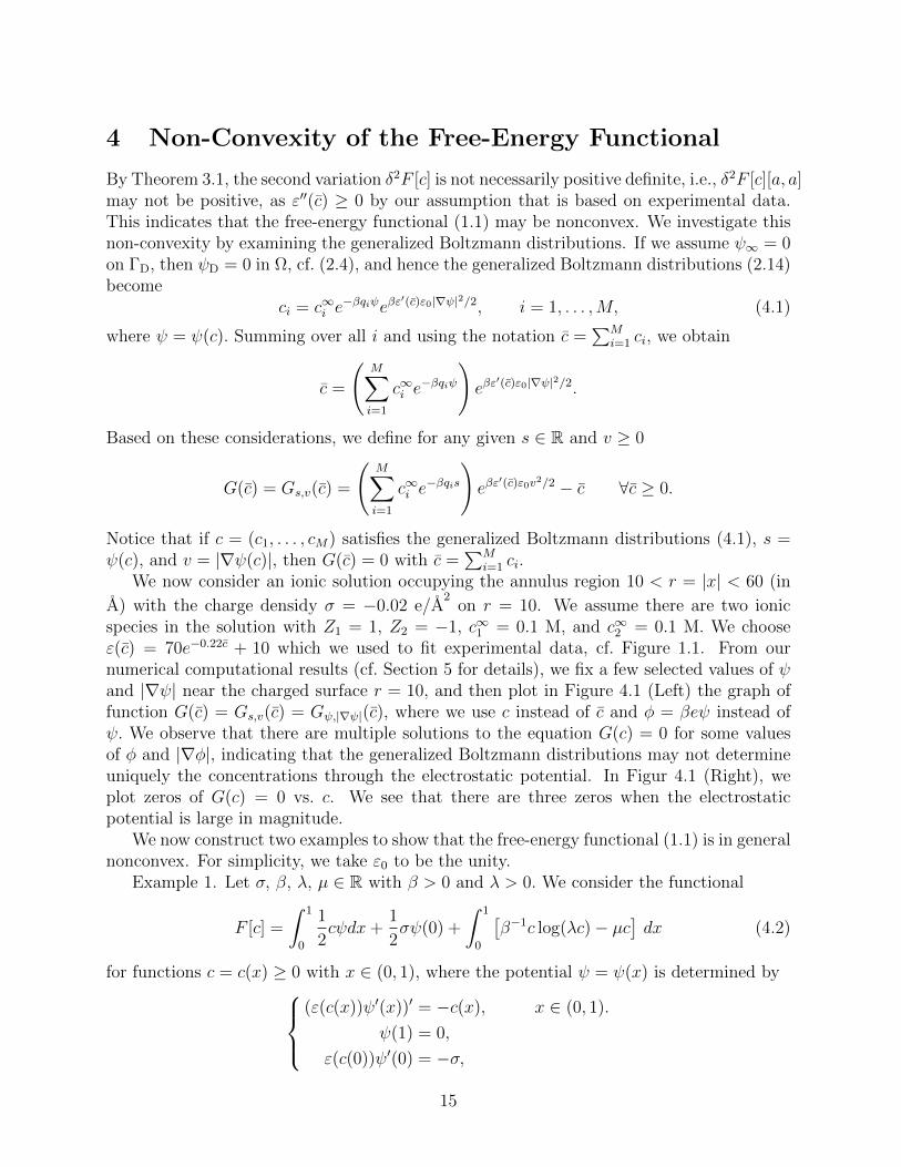
on r = 10. We assume there are two ionicspecies in the solution with Z1 = 1, Z2 = −1, c∞1 = 0.1 M, and c∞2 = 0.1 M. We chooseε(c) = 70e−0.22c + 10 which we used to fit experimental data, cf. Figure 1.1. From ournumerical computational results (cf. Section 5 for details), we fix a few selected values of ψand |∇ψ| near the charged surface r = 10, and then plot in Figure 4.1 (Left) the graph offunction G(c) = Gs,v(c) = Gψ,|∇ψ|(c), where we use c instead of c and φ = βeψ instead ofψ. We observe that there are multiple solutions to the equation G(c) = 0 for some valuesof φ and |∇φ|, indicating that the generalized Boltzmann distributions may not determineuniquely the concentrations through the electrostatic potential. In Figur 4.1 (Right), weplot zeros of G(c) = 0 vs. c. We see that there are three zeros when the electrostaticpotential is large in magnitude.
We now construct two examples to show that the free-energy functional (1.1) is in generalnonconvex. For simplicity, we take ε0 to be the unity.
Example 1. Let σ, β, λ, µ ∈ R with β > 0 and λ > 0. We consider the functional
F [c] =
∫ 1
0
1
2cψdx+
1
2σψ(0) +
∫ 1
0
[β−1c log(λc)− µc
]dx (4.2)
for functions c = c(x) ≥ 0 with x ∈ (0, 1), where the potential ψ = ψ(x) is determined by(ε(c(x))ψ′(x))′ = −c(x), x ∈ (0, 1).
ψ(1) = 0,
ε(c(0))ψ′(0) = −σ,
15
0 5 10 15−5
−4
−3
−2
−1
0
1
2
c
G(c
)
0φ = −5.0; |∇φ| = 1.35/A−1
φ = −5.0; |∇φ| = 1.30/A−1
φ = −5.0; |∇φ| = 1.20/A−1
φ = −4.9; |∇φ| = 1.35/A−1
φ = −4.9; |∇φ| = 1.29/A−1
−7−6
−5−4
−3−2
−10
0
1
2
3
4
5
0
5
10
15
20
25
30
35
40
45
50
φ|∇φ|
Zero
s o
f G
(c)
Figure 4.1: Left: G(c) vs. c for different values of φ and |∇φ|. Right: Zeros of G(c) vs. φand |∇φ|. The three dots on the verticle line indicate the three zeros of G(c).
Here, ε(c) = 70e−0.22c+10, which was used to fit experimental data in Figure 1.1. This modelcan be viewed as reduced from a three-dimensional model with the ionic concentration andelectrostatic potential only varying in the x-coordinate direction.
If c is a constant function, then we have by simple calculations that
ψ(x) = − cx2
2ε(c)− σx
ε(c)+
c
2ε(c)+
σ
ε(c), x ∈ (0, 1),
F [c] =c2 + 3cσ + 3σ2
6ε(c)+ β−1c log
( c
c∞
), c > 0, (4.3)
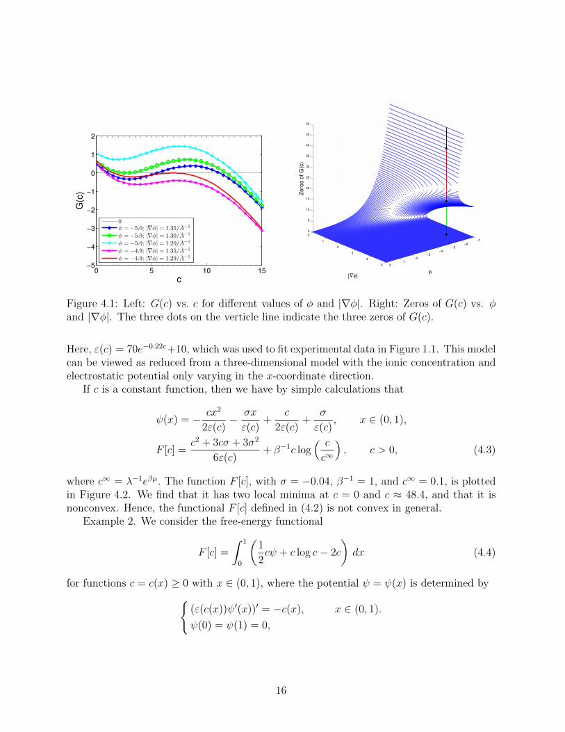
where c∞ = λ−1eβµ. The function F [c], with σ = −0.04, β−1 = 1, and c∞ = 0.1, is plottedin Figure 4.2. We find that it has two local minima at c = 0 and c ≈ 48.4, and that it isnonconvex. Hence, the functional F [c] defined in (4.2) is not convex in general.
Example 2. We consider the free-energy functional
F [c] =
∫ 1
0
(1
2cψ + c log c− 2c
)dx (4.4)
for functions c = c(x) ≥ 0 with x ∈ (0, 1), where the potential ψ = ψ(x) is determined by(ε(c(x))ψ′(x))′ = −c(x), x ∈ (0, 1).
ψ(0) = ψ(1) = 0,
16

0 20 40 60 80 1000
200
400
600
800
1000
c (M)
F[c]
Figure 4.2: Graph of the function F [c] defined in (4.3).
The function ε = ε(c) is defined by
ε(c) =
1025
36− 50
9c if 0 ≤ c < 4,
25
18(c− 6)2 +
25
36if 4 ≤ c < 6,
25
36if 6 ≤ c <∞.
(4.5)
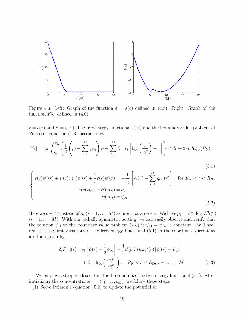
It can be verified that this is a C1-function, monotonically decreasing, convex, and boundedabove and below by positive constants. See Figure 4.3 (Left) for a plot of this function.
For constant functions c, we have
ψ(x) = − cx2
2ε(c)+
cx
2ε(c), x ∈ (0, 1),
F [c] =c2
24ε(c)+ c log(c)− 2c, c > 0. (4.6)
Figure 4.3 (Right) is a plot of the function F [c] defined in (4.6). We see clearly that thisfunction F [c] is not convex. Hence the functional F [c] defined in (4.4) is not convex.
5 Numerical Study of a Model System
We minimize numerically the free-energy functional (1.1) and (1.3) with
Ω = x ∈ R3 : RN < |x| < RD, ΓN = x ∈ R3 : |x| = RN, ΓD = x ∈ R3 : |x| = RD,
where RD and RN are two given positive numbers such that RD < RN. We assume thatρf = ρf(r) is a function of r = |x|, ψ∞ is a constant, and σ is also a constant. By the radialsymmetry, we assume the concentrations and potential are functions of r = |x| and write
17
0 5 10 15 200
5
10
15
20
c (M)
ε(c)
0 5 10 15 20−15
−10
−5
0
5
c (M)
F[c]
Figure 4.3: Left: Graph of the function ε = ε(c) defined in (4.5). Right: Graph of thefunction F [c] defined in (4.6).
c = c(r) and ψ = ψ(r). The free-energy functional (1.1) and the boundary-value problem ofPoisson’s equation (1.3) become now
F [c] = 4π
∫ RD
RN
1
2
(ρf +
M∑i=1
qici
)ψ +
M∑i=1
β−1ci
[log
(cic∞i
)− 1
]r2 dr + 2πσR2
Nψ(RN),
(5.1)ε(c)ψ′′(r) + ε′(c)c′(r)ψ′(r) +
2
rε(c)ψ′(r) = − 1
ε0
[ρf(r) +
M∑i=1
qici(r)
]for RN < r < RD,
−ε(c(RN))ε0ψ′(RN) = σ,
ψ(RD) = ψ∞.
(5.2)
Here we use c∞i instead of µi (i = 1, . . . ,M) as input parameters. We have µi = β−1 log(Λ3c∞i )(i = 1, . . . ,M). With our radially symmetric setting, we can easily observe and verify thatthe solution ψD to the boundary-value problem (2.3) is ψD = ψ∞, a constant. By Theo-rem 2.1, the first variations of the free-energy functional (5.1) in the coordinate directionsare then given by
δiF [c](r) =qi
[ψ(r)− 1
2ψ∞
]− 1
2ε′(c(r))ε0ψ
′(r) [ψ′(r)− ψ∞]
+ β−1 log
(ci(r)
c∞i
), RN < r < RD, i = 1, . . . ,M. (5.3)
We employ a steepest descent method to minimize the free-energy functional (5.1). Afterinitializing the concentrations c = (c1, . . . , cM), we follow these steps:
(1) Solve Poisson’s equation (5.2) to update the potential ψ.
18

(2) Compute the first variations δiF [c] (i = 1, . . . ,M) by (5.3).(3) Update the concentrations: ci ← ci − γdi (i = 1, . . . ,M), where γ > 0 is a pre-chosen
parameter.(4) Check if max1≤i≤M ‖δiF [c]‖L∞(RN,RD) < εtol with a pre-chosen tolerance εtol. If not, go
back to (1).We choose the parameter γ in Step (3) to be very small to ensure that all ci > 0 in eachiteration. In case ci < 0 for some i, we can change γ to a smaller value to update ci. Notethat we only find numerically local minimizers that are sometimes more interesting in termsof physical properties than global minimizers.
We now fixRN = 10 A andRD = 60 A, and vary the surface charge density σ from−0.005
to −0.025 e/A2. As surface charges generally represent the main part of fixed charges, we
set ρf = 0. Moreover, since we are mainly interested in the counterion concentrations andelectrostatic potentials near the charged surface, we set ψ∞ = 0. We use kBT as units ofenergy. We consider two systems.
System I: M = 2, Z1 = 1, Z2 = −1, c∞1 = 0.1 M, and c∞2 = 0.1 M.System II: M = 3, Z1 = 2, Z2 = 1, Z3 = −2, c∞1 = 0.1 M, c∞2 = 0.1 M, c∞3 = 0.15 M.
In each of our numerical computations, we observe the decay of the free energy and theconvergence of concentrations in our iterations. This indicates that our numerical methodis reliable.
5.1 Comparison of Different Dielectric Relations: Counterion De-pletion
We compare equilibrium concentrations and electrostatic potentials corresponding to thefollowing four different dielectric coefficient functions ε = εi(c) : (c ≥ 0):
ε1(c) = 80; ε2(c) = 80− 20c; ε3(c) =80
1 + 0.25c; ε4(c) = 70e−0.22c + 10. (5.4)
Note that all these functions are convex and monotonically decreasing with the maximumvalue 80 at c = 0. In addition ε3(∞) = 0 and ε4(∞) = 10. The linear dependence ε2(c) isused in [7]. The form ε3(c) is proposed in [31]. We used ε4(c) to fit the experiment data inFigure 1.1.
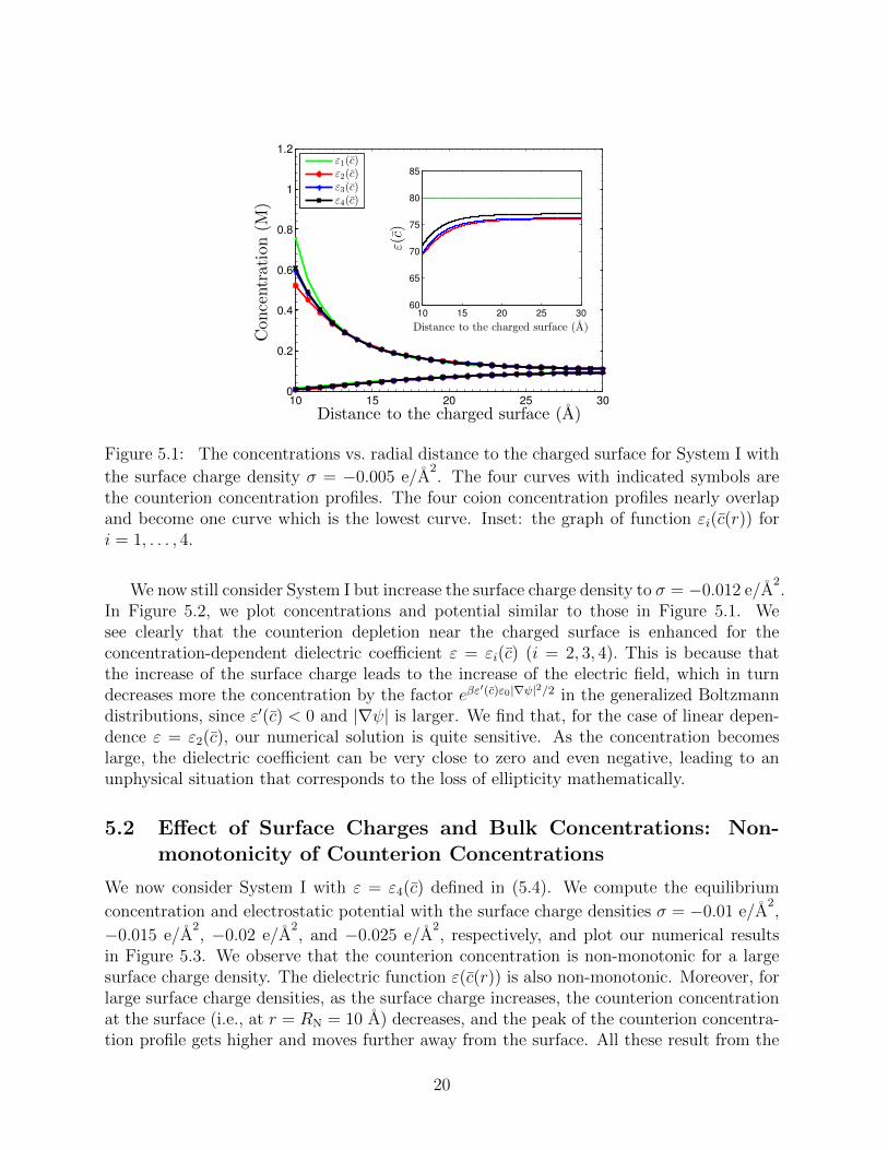
We consider System I with the surface charge density σ = −0.005 e/A2. In Figure 5.1,
we plot profiles of the equilibrium concentrations for both counterion and coion species forthe four different dielectric coefficient defined in (5.4). The four concentration profiles forthe species of coions nearly overlap and become one. It is the curve below all the other fourfor the counterion concentrations. The inset shows the graph of εi(c(r)) (1 ≤ i ≤ 4) as afunction of the radial variable r. We observe differences of the counterion concentrationsin the vicinity of the charged surface, even at such a relatively low surface charge density.The counterion concentrations corresponding to ε2(c), ε3(c), and ε4(c) are smaller than thatpredicted by the classical PB theory that corresponds to ε1(c). Such counterion depletionis expected as explained in Introduction and as found in [7].
19
10 15 20 25 300
0.2
0.4
0.6
0.8
1
1.2
Distance to the charged surface (A)
Concentration(M
)
ε1(c)ε2(c)ε3(c)ε4(c)
10 15 20 25 3060
65
70
75
80
85
Distance to the charged surface (A)
ε(c)
Figure 5.1: The concentrations vs. radial distance to the charged surface for System I with
the surface charge density σ = −0.005 e/A2. The four curves with indicated symbols are
the counterion concentration profiles. The four coion concentration profiles nearly overlapand become one curve which is the lowest curve. Inset: the graph of function εi(c(r)) fori = 1, . . . , 4.
We now still consider System I but increase the surface charge density to σ = −0.012 e/A2.
In Figure 5.2, we plot concentrations and potential similar to those in Figure 5.1. Wesee clearly that the counterion depletion near the charged surface is enhanced for theconcentration-dependent dielectric coefficient ε = εi(c) (i = 2, 3, 4). This is because thatthe increase of the surface charge leads to the increase of the electric field, which in turndecreases more the concentration by the factor eβε
′(c)ε0|∇ψ|2/2 in the generalized Boltzmanndistributions, since ε′(c) < 0 and |∇ψ| is larger. We find that, for the case of linear depen-dence ε = ε2(c), our numerical solution is quite sensitive. As the concentration becomeslarge, the dielectric coefficient can be very close to zero and even negative, leading to anunphysical situation that corresponds to the loss of ellipticity mathematically.
5.2 Effect of Surface Charges and Bulk Concentrations: Non-monotonicity of Counterion Concentrations
We now consider System I with ε = ε4(c) defined in (5.4). We compute the equilibrium
concentration and electrostatic potential with the surface charge densities σ = −0.01 e/A2,
−0.015 e/A2, −0.02 e/A
2, and −0.025 e/A
2, respectively, and plot our numerical results
in Figure 5.3. We observe that the counterion concentration is non-monotonic for a largesurface charge density. The dielectric function ε(c(r)) is also non-monotonic. Moreover, forlarge surface charge densities, as the surface charge increases, the counterion concentrationat the surface (i.e., at r = RN = 10 A) decreases, and the peak of the counterion concentra-tion profile gets higher and moves further away from the surface. All these result from the
20

10 15 20 25 300
1
2
3
4
5
6
7
Distance to the charged surface (A)
Concentration(M
)
ε1(c)ε2(c)ε3(c)ε4(c)
10 15 20 25 3055
60
65
70
75
80
85
Distance to the charged surface (A)
ε(c)
Figure 5.2: The concentrations vs. radial distance to the charged surface for System I with
the surface charge density σ = −0.012 e/A2. The four curves with indicated symbols are
the counterion concentration profiles. The four coion concentration profiles nearly overlapand become one curve which is the lowest curve. Inset: the graph of function εi(c(r)) fori = 1, . . . , 4.
competition between the surface-counterion attraction and the counterion depletion nearthe surface.
10 15 20 25 300
0.5
1
1.5
2
2.5
3
3.5
Distance to the charged surface (A)
Concentration(M
)
σ = −0.01e/A2
σ = −0.015e/A2
σ = −0.02e/A2
σ = −0.025e/A2
10 15 20 25 3050
55
60
65
70
75
80
Distance to the charged surface (A)
ε(c)
10 15 20 25 30
−12
−10
−8
−6
−4
−2
0
Distance to the charged surface (A)
Eletrostaticpotential
σ = −0.01e/A2
σ = −0.015e/A2
σ = −0.02e/A2
σ = −0.025e/A2
Figure 5.3: System I with ε = ε4(c). Left: The ionic concentrations vs. the radial distanceto the charged surface. The four counterion concentration profiles for the four differentvalues of the surface charge density are indicated by the symbols. The four correspondingcoion concentrations overlap and become one curve which is the lowest one. Right: Theelectrostatic potentials vs. the radial distance to the charged surface for different values ofthe surface charge density.
21
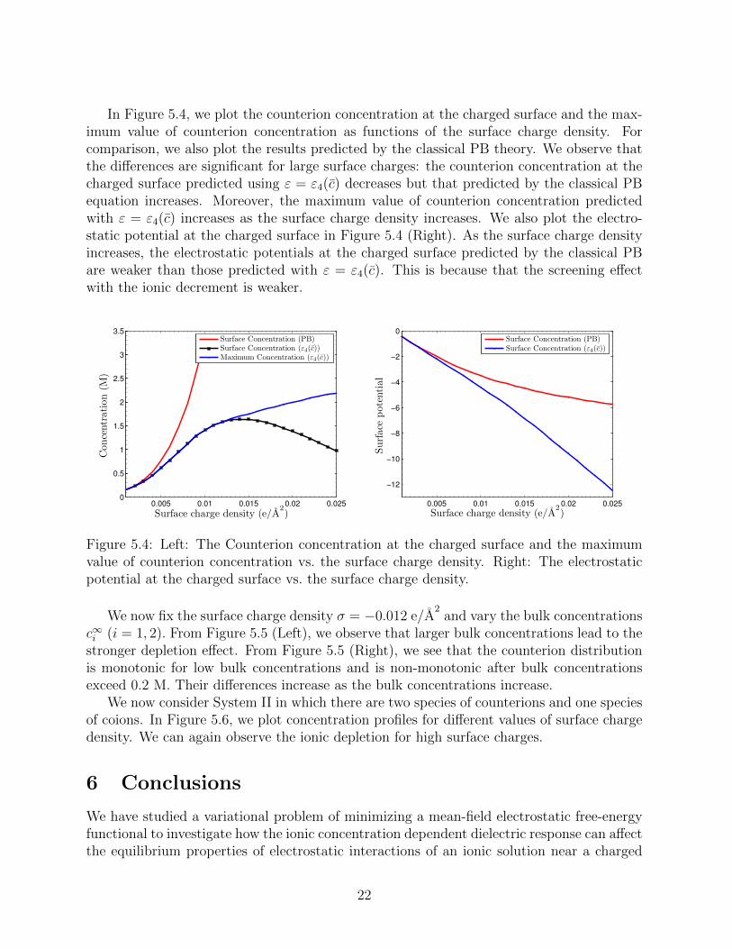
In Figure 5.4, we plot the counterion concentration at the charged surface and the max-imum value of counterion concentration as functions of the surface charge density. Forcomparison, we also plot the results predicted by the classical PB theory. We observe thatthe differences are significant for large surface charges: the counterion concentration at thecharged surface predicted using ε = ε4(c) decreases but that predicted by the classical PBequation increases. Moreover, the maximum value of counterion concentration predictedwith ε = ε4(c) increases as the surface charge density increases. We also plot the electro-static potential at the charged surface in Figure 5.4 (Right). As the surface charge densityincreases, the electrostatic potentials at the charged surface predicted by the classical PBare weaker than those predicted with ε = ε4(c). This is because that the screening effectwith the ionic decrement is weaker.
0.005 0.01 0.015 0.02 0.0250
0.5
1
1.5
2
2.5
3
3.5
Surface charge density (e/A2)
Concentration(M
)
Surface Concentration (PB)Surface Concentration (ε4(c))Maximum Concentration (ε4(c))
0.005 0.01 0.015 0.02 0.025
−12
−10
−8
−6
−4
−2
0
Surface charge density (e/A2)
Surface
potential
Surface Concentration (PB)Surface Concentration (ε4(c))
Figure 5.4: Left: The Counterion concentration at the charged surface and the maximumvalue of counterion concentration vs. the surface charge density. Right: The electrostaticpotential at the charged surface vs. the surface charge density.
We now fix the surface charge density σ = −0.012 e/A2
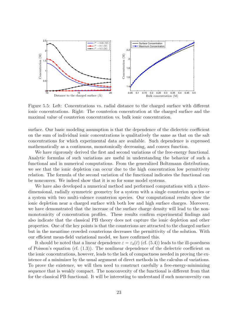
and vary the bulk concentrationsc∞i (i = 1, 2). From Figure 5.5 (Left), we observe that larger bulk concentrations lead to thestronger depletion effect. From Figure 5.5 (Right), we see that the counterion distributionis monotonic for low bulk concentrations and is non-monotonic after bulk concentrationsexceed 0.2 M. Their differences increase as the bulk concentrations increase.
We now consider System II in which there are two species of counterions and one speciesof coions. In Figure 5.6, we plot concentration profiles for different values of surface chargedensity. We can again observe the ionic depletion for high surface charges.
6 Conclusions
We have studied a variational problem of minimizing a mean-field electrostatic free-energyfunctional to investigate how the ionic concentration dependent dielectric response can affectthe equilibrium properties of electrostatic interactions of an ionic solution near a charged
22
10 15 200
0.5
1
1.5
2
2.5
Distance to the charged surface (A)
Concentration(M
)
c∞ = 0.05 (M)c∞ = 0.1 (M)c∞ = 0.5 (M)
0.05 0.1 0.15 0.2 0.25 0.3 0.35 0.4 0.45 0.5
1.4
1.6
1.8
2
2.2
Bulk concentration (M)
Concentration(M
)
Surface Concentration
Maximum Concentration
Figure 5.5: Left: Concentrations vs. radial distance to the charged surface with differentionic concentrations. Right: The counterion concentration at the charged surface and themaximal value of counterion concentration vs. bulk ionic concentration.
surface. Our basic modeling assumption is that the dependence of the dielectric coefficienton the sum of individual ionic concentrations is qualitatively the same as that on the saltconcentrations for which experimental data are available. Such dependence is expressedmathematically as a continuous, monotonically decreasing, and convex function.
We have rigorously derived the first and second variations of the free-energy functional.Analytic formulas of such variations are useful in understanding the behavior of such afunctional and in numerical computations. From the generalized Boltzmann distributions,we see that the ionic depletion can occur due to the high concentration low permittivityrelation. The formula of the second variation of the functional indicates the functional canbe nonconvex. We indeed show that it is so for some model systems.
We have also developed a numerical method and performed computations with a three-dimensional, radially symmetric geometry for a system with a single counterion species ora system with two multi-valence counterion species. Our computational results show theionic depletion near a charged surface with both low and high surface charges. Moreover,we have demonstrated that the increase of the surface charge density will lead to the non-monotonicity of concentration profiles. These results confirm experimental findings andalso indicate that the classical PB theory does not capture the ionic depletion and otherproperties. One of the key points is that the counterions are attracted to the charged surfacebut in the meantime crowded counterions decreases the permittivity of the solution. Withour efficient mean-field variational model, we have confirmed this.
It should be noted that a linear dependence ε = ε2(c) (cf. (5.4)) leads to the ill-posednessof Poisson’s equation (cf. (1.3)). The nonlinear dependence of the dielectric coefficient onthe ionic concentrations, however, leads to the lack of compactness needed in proving the ex-istence of a minimizer by the usual argument of direct methods in the calculus of variations.To prove the existence, we will then need to construct carefully a free-energy-minimizingsequence that is weakly compact. The nonconvexity of the functional is different from thatfor the classical PB functional. It will be interesting to understand if such nonconvexity can
23

10 15 200
0.1
0.2
0.3
0.4
0.5
0.6
0.7
0.8
0.9
1
Distance to the charged surface (A)
Concentration(M
)
Z1 = +2Z2 = +1Z3 = −1
10 15 200
0.5
1
1.5
2
2.5
3
3.5
Distance to the charged surface (A)
Concentration(M
)
Z1 = +2Z2 = +1Z3 = −1
10 15 200
0.5
1
1.5
2
2.5
3
3.5
Distance to the charged surface (A)
Concentration(M
)
Z1 = +2Z2 = +1Z3 = −1
10 15 200
0.5
1
1.5
2
2.5
3
3.5
Distance to the charged surface (A)
Concentration(M
)
Z1 = +2Z2 = +1Z3 = −1
Figure 5.6: Ionic concentrations vs. radial distance to the charge surface with different values
of surface charge density σ. Upper left: σ = −0.005e/A2. Upper right: σ = −0.01e/A
2.
Lower left: σ = −0.015e/A2. Lower right: σ = −0.02e/A
2.
be used to model the transition from weak to strong interactions in an ionic solution.Our numerical algorithm is fairly general. The key of our algorithm is the self-consistency:
In each step of relaxing the free-energy functional, we solve Poisson’s equation with the con-centration dependent dielectric coefficient. We update the concentrations and electrostaticpotential alternatively. If one simply uses the classical Boltzmann distributions for ci’s inε = ε(c), one may not be able to capture the ionic depletion as shown in the recent work [38].
One of the ion-specific properties is the ionic size effect. In recent years, the PB-likemean-field models that account for ionic size effects have been developed [5, 7, 8, 22, 35–37,39,55,59,61]. Our experience is that a large (in terms of magnitude) surface charge densityis needed to capture the ionic size effect in such models, while only a small charge density isneeded to capture the ionic decrement near a charged surface. It will be therefore interestingto see the transition characterized by the surface charge density. Another important issuethat we have not addressed here is the Born solvation energy of ions [41,56,60]. Additionalequations may be needed to describe such energy. It is interesting to understand whether
24
the inclusion of the Born solvation energy will also lead to the correction term in thegeneralized Boltzmann distributions. Finally, in terms of applications, how to apply ourresults to modeling charged macromolecules, such as proteins, in an aqueous environmentis of great interest.
Acknowledgments. This work was supported by the US National Science Foundation(NSF) through the grant DMS-131973, the NSF Center for Theoretical Biological Physicsthrough the grant PHY-0822283, the US National Institutes of Health through the grantR01GM096188, and a UCSD Chancellor’s Interdisciplinary Collaboratories grant. The au-thors thank Dr. Joachim Dzubiella, Dr. Zhenli Xu, Dr. Zhongming Wang, and Dr. YanxiangZhao for many helpful discussions. The authors also thank the anonymous referees for theirhelpful comments and suggestions.
References
[1] A. Abrashkin, D. Andelman, and H. Orland. Dipolar Poisson–Boltzmann equation:Ions and dipoles close to charge interfaces. Phys. Rev. Lett., 99:077801, 2007.
[2] R. Adams. Sobolev Spaces. Academic Press, New York, 1975.
[3] D. Andelman. Electrostatic properties of membranes: The Poisson–Boltzmann theory.In R. Lipowsky and E. Sackmann, editors, Handbook of Biological Physics, volume 1,pages 603–642. Elsevier, 1995.
[4] D. Andelman. Introduction to electrostatics in soft and biological matter. In W. Poonand D. Andelman, editors, Proceedings of the Nato ASI & SUSSP on “Soft condensedmatter physics in molecular and cell biology” (2005), pages 97–122, New York, 2006.Taylor & Francis.
[5] D. Ben-Yaakov, D. Andelman, D. Harries, and R. Podgornik. Beyond standardPoisson–Boltzmann theory: Ion-specific interactions in aqueous solutions. J. Phys.:Condens. Matter, 21:424106, 2009.
[6] D. Ben-Yaakov, D. Andelman, D. Harries, and R. Podgornik. Ions in mixed dielectricsolvents: Density profiles and osmotic pressure between charged interfaces. J. Phys.Chem. B, 113:6001–6011, 2009.
[7] D. Ben-Yaakov, D. Andelman, and R. Podgornik. Dielectric decrement as a source ofion-specific effects. J. Chem. Phys., 134:074705, 2011.
[8] I. Borukhov, D. Andelman, and H. Orland. Steric effects in electrolytes: A modifiedPoisson–Boltzmann equation. Phys. Rev. Lett., 79:435–438, 1997.
[9] R. Buchner, G. T. Hefter, and J. Barthel. Dielectric relaxation of aqueous NaF andKF solutions. J. Chem. Soc. Faraday Trans., 90:2475–2479, 1994.
25

[10] R. Buchner, G. T. Hefter, and P. M. May. Dielectric relaxation of aqueous NaClsolutions. J. Phys. Chem. A, 103:1–9, 1999.
[11] D. L. Chapman. A contribution to the theory of electrocapillarity. Philos. Mag.,25:475–481, 1913.
[12] J. Che, J. Dzubiella, B. Li, and J. A. McCammon. Electrostatic free energy and itsvariations in implicit solvent models. J. Phys. Chem. B, 112:3058–3069, 2008.
[13] M. E. Davis and J. A. McCammon. Electrostatics in biomolecular structure and dy-namics. Chem. Rev., 90:509–521, 1990.
[14] P. Debye and E. Huckel. Zur Theorie der Elektrolyte. Physik. Zeitschr., 24:185–206,1923.
[15] V. Demery, D. S. Dean, and R. Podgornik. Electrostatic interactions mediated bypolarizable counterions: Weak and strong coupling limits. J. Chem. Phys., 137:174903,2012.
[16] K. A. Dill. Dominant forces in protein folding. Biochemistry, 29:7133–7155, 1990.
[17] P. Drude and W. Nernst. Uber Elektrostriktion durch freie Ionen. Z. Phys. Chem.,15:79–85, 1984.
[18] L. C. Evans. Partial Differential Equations, volume 19 of Graduate Studies in Mathe-matics. Amer. Math. Soc., 2nd edition, 2010.
[19] F. Fixman. The Poisson–Boltzmann equation and its application to polyelecrolytes. J.Chem. Phys., 70:4995–5005, 1979.
[20] F. Fogolari and J. M. Briggs. On the variational approach to Poisson–Boltzmann freeenergies. Chem. Phys. Lett., 281:135–139, 1997.
[21] F. Fogolari, A. Brigo, and H. Molinari. The Poisson–Boltzmann equation for biomolec-ular electrostatics: a tool for structural biology. J. Mol. Recognit., 15:377–392, 2002.
[22] D. Frydel. Polarizable Poisson–Boltzmann equation: The study of polarizability effectson the structure of a double layer. J. Chem. Phys., 134:234704, 2011.
[23] D. Gilbarg and N. S. Trudinger. Elliptic Partial Differential Equations of Second Order.Springer-Verlag, 2nd edition, 1998.
[24] M. Gouy. Sur la constitution de la charge electrique a la surface d’un electrolyte. J.Phys. Theor. Appl., 9:457–468, 1910.
[25] P. Grochowski and J. Trylska. Continuum molecular electrostatics, salt effects andcounterion binding—A review of the Poisson–Boltzmann model and its modifications.Biopolymers, 89:93–113, 2008.
26
[26] J. B. Hasted. Aqueous Dielectrics. Chapman and Hall, London, 1973.
[27] J. B. Hasted, D. M. Riston, and C. H. Collie. Dielectric properties of aqueous ionicsolutions. Parts I and II. J. Chem. Phys., 16:1–21, 1948.
[28] B. Hille. Ion Channels of Excitable Membranes. Sinauer Associates, 3rd edition, 2001.
[29] B. Honig and A. Nicholls. Classical electrostatics in biology and chemistry. Science,268:1144–1149, 1995.
[30] J. D. Jackson. Classical Electrodynamics. Wiley, New York, 3rd edition, 1999.
[31] I. Kalcher and J. Dzubiella. Structure-thermodynamics relation of electrolyte solutions.J. Chem. Phys., 130:134507, 2009.
[32] L. D. Landau, E. M. Lifshitz, and L. P. Pitaevski. Electrodynamics of ContinuousMedia. Butterwort–Heinemann, 2nd edition, 1993.
[33] R. T. Lattey. The dielectric constants of electrolytic solutions. Philos. Mag., 41:829–848, 1921.
[34] A. Levy, D. Andelman, and H. Orland. Dielectric constant of ionic solutions: A field-theory approach. Phys. Rev. Lett., 108:227801, 2012.
[35] B. Li. Continuum electrostatics for ionic solutions with nonuniform ionic sizes. Non-linearity, 22:811–833, 2009.
[36] B. Li. Minimization of electrostatic free energy and the Poisson–Boltzmann equationfor molecular solvation with implicit solvent. SIAM J. Math. Anal., 40:2536–2566,2009.
[37] B. Li, P. Liu, Z. Xu, and S. Zhou. Ionic size effects: generalized boltzmann distributions,counterion stratification, and modified debye length. Nonlinearity, 26:2899–2922, 2013.
[38] H. Li and B. Lu. An ionic concentration and size dependent dielectric permittiv-ity Poisson–Boltzmann model for biomolecular solvation studies. J. Chem. Phys.,141:024115, 2014.
[39] B. Z. Lu and Y. C. Zhou. Poisson–Nernst–Planck equations for simulating biomoleculardiffusion-reaction processes II: Size effects on ionic distributions and diffusion-reactionrates. Biophys J., 100:2475–2485, 2011.
[40] A. K. Lyashchenko and A. Yu. Zasetsky. Complex dielectric permittivity and relaxationparameters of concentrated aqueous electrolyte solutions in millimeter and centimeterwavelength ranges. J. Molecular Liquids, 77:61–75, 1998.
[41] M. Ma and Z. Xu. Self-consistent field model for strong electrostatic correlations andinhomogeneous dielectric media. J. Chem. Phys., 2014 (in press).
27
[42] J. A. McCammon. Darwinian biophysics: Electrostatics and evolution in the kineticsof molecular binding. Proc. Nat. Acad. Sci. USA., 106:7683–7684, 2009.
[43] S. McLaughlin. The electrostatic properties of membranes. Annu. Rev. Biophys. Bio-phys. Chem., 18:113–136, 1989.
[44] R. Messina. Electrostatics in soft matter. J. Phys.: Condens. Matter, 21:113102, 2009.
[45] A. Naji, M. Kandu, J. Forsman, and R. Podgornik. Perspective: Coulomb fluidsweakcoupling, strong coupling, in between and beyond. J. Chem. Phys., 139:150901, 2013.
[46] I. Nakamura, A.-C. Shi, and Z.-G. Wang. Ion solvation in liquid mixtures: Effects ofsolvent reorganization. Phys. Rev. Lett., 109:257802, 2012.
[47] K. Nortemann, J. Hilland, and U. Kaatze. Dielectric properties of aqueous NaCl solu-tions at microwave frequencies. J. Phys. Chem. A, 101:6864–6869, 1997.
[48] O. I. Obolensky, T. P. Doerr, R. Ray, and Y.-K. Yu. Rigorous treatment of electrostaticsfor spatially varying dielectrics based on energy minimization. Phys. Rev. E, 79:041907,2009.
[49] E. S. Reiner and C. J. Radke. Variational approach to the electrostatic free energy incharged colloidal suspensions: general theory for open systems. J. Chem. Soc. FaradayTrans., 86:3901–3912, 1990.
[50] R. Renou, M. Ding, H. Zhu, A. Szymczyk, P. Malfreyt, and A. Ghoufi. Concentrationdependence of the dielectric permittivity, structure, and dynamics of aqueous NaClsolutions: Comparison between the Drude oscillator and electronic continuum models.J. Phys. Chem. B, 118:3931–3940, 2014.
[51] J. Sala, E. Guadia, and J. Marti. Effects of concentration on structure, dielectric, anddynamic properties of aqueous NaCl solutions using a polarizable model. J. Chem.Phys., 132:214505, 2010.
[52] C. C. Schmidt. The dielectric constants of four electrolytes as given by the Carmanelectrometer method. Phys. Rev., 30:925–930, 1927.
[53] K. A. Sharp and B. Honig. Electrostatic interactions in macromolecules: Theory andapplications. Annu. Rev. Biophys. Biophys. Chem., 19:301–332, 1990.
[54] F. B. Sheinerman, R. Norel, and B. Honig. Electrostatic aspects of protein-proteininteractions. Curr. Opin. Struct. Biology, 10:153–159, 2000.
[55] G. Tresset. Generalized Poisson–Fermi formalism for investigating size correlationeffects with multiple ions. Phys. Rev. E, 78:061506, 2008.
[56] Z.-G. Wang. Fluctuation in electrolyte solutions: The self energy. Phys. Rev. E,81:021501, 2010.
28
[57] Y. Wei and S. Sridhar. Dielectric spectroscopy up to 20 GHz of LiCl/H2O solutions.J. Chem. Phys., 92:923–926, 1990.
[58] Y.-Z. Wei, P. Chiang, and S. Sridhar. Ion size effects on the dynamic and staticdielectric properties of aqueous alkali solutions. J. Chem. Phys., 96:4569–4573, 1992.
[59] J. Wen, S. Zhou, Z. Xu, and B. Li. Competitive adsorption and ordered packingof counterions near highly charged surfaces: From mean-field theory to Monte Carlosimulations. Phys. Rev. E, 85:041406, 2012.
[60] Z. Xu, M. Ma, and P. Liu. Self-energy modified Poisson–Nernst–Planck equations:WKB approximation and finite-difference approaches. Phys. Rev. E, 90:013307, 2014.
[61] S. Zhou, Z. Wang, and B. Li. Mean-field description of ionic size effects with non-uniform ionic sizes: A numerical approach. Phys. Rev. E, 84:021901, 2011.
29