ME751 Advanced Computational

Multibody Dynamics

RK-Methods

AB & AM Methods

BDF MethodsMarch 25, 2010

© Dan Negrut, 2010ME751, UW-Madison

“A Constitution should be short and obscure.”Napoleon Bonaparte

Before we get started…

Last Time: Numerical solution of IVP

Basic Concepts: truncation error, accuracy, zero-stability, convergence, local error, stability

Today: Finish discussion of Basic Concepts

Concentrate on Implicit Integration: why it’s hard, and what it buys you

Basic Methods Skip altogether Runge-Kutta, Adams-Bashforth, and Adams-Moulton Methods Cover BDF methods

New HW uploaded on the class website It’s ugly

Trip to John Deere & NADS: need head count by April 8 – email me Transportation and hotel will be covered Leave on May 3 at 6 pm or so, return on May 4 at 10 pm Might also visit software company in Iowa City, they have a simulation tool just like ADAMS

2

Implicit Methods

Implicit methods were derived to answer the limitation on the step size noticed for Forward Euler, which is an explicit method

Simplest implicit method: Backward Euler Given the IVP

Backward Euler finds at each time step tn the solution by solving the following equation for yn:

3

Explicit vs. Implicit Methods

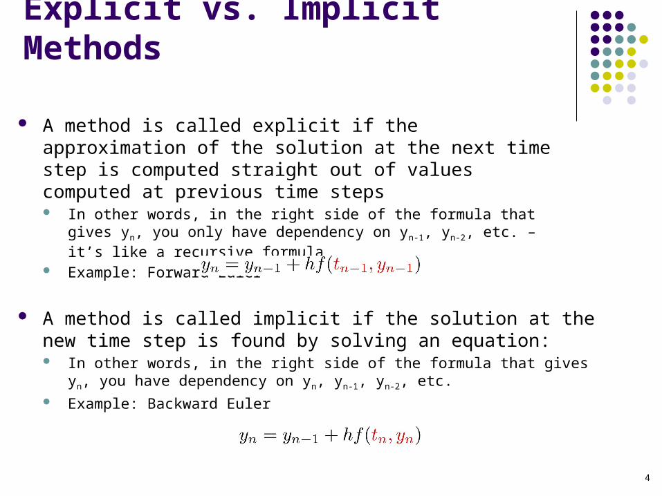
A method is called explicit if the approximation of the solution at the next time step is computed straight out of values computed at previous time steps In other words, in the right side of the formula that gives yn, you only have

dependency on yn-1, yn-2, etc. – it’s like a recursive formula Example: Forward Euler

4

A method is called implicit if the solution at the new time step is found by solving an equation: In other words, in the right side of the formula that gives yn, you have dependency

on yn, yn-1, yn-2, etc. Example: Backward Euler

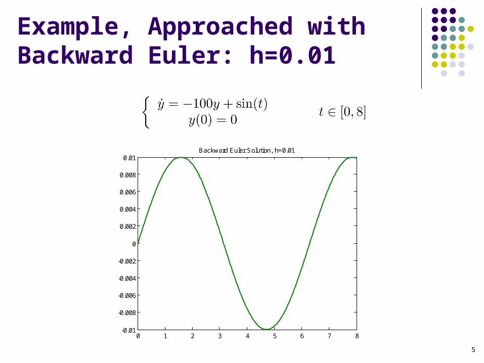
Example, Approached with Backward Euler: h=0.01

5

0 1 2 3 4 5 6 7 8-0.01

-0.008

-0.006

-0.004

-0.002

0

0.002

0.004

0.006

0.008

0.01Backward Euler Solution, h=0.01

Example, Approached with Backward Euler: h=0.02

6

0 1 2 3 4 5 6 7 8-0.01

-0.008

-0.006

-0.004

-0.002

0

0.002

0.004

0.006

0.008

0.01Backward Euler Solution, h=0.02

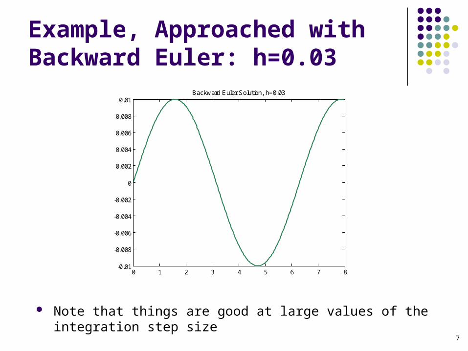
Example, Approached with Backward Euler: h=0.03

7

Note that things are good at large values of the integration step size

0 1 2 3 4 5 6 7 8-0.01

-0.008

-0.006

-0.004

-0.002

0

0.002

0.004

0.006

0.008

0.01Backward Euler Solution, h=0.03

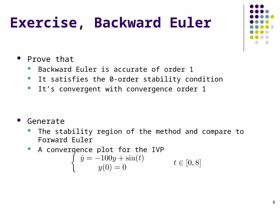
Exercise, Backward Euler

Prove that Backward Euler is accurate of order 1 It satisfies the 0-order stability condition It’s convergent with convergence order 1

Generate The stability region of the method and compare to Forward Euler A convergence plot for the IVP

8

Stability Region, Backward Euler

9

Generating Convergence Plot

Procedure to generate Convergence Plot: First, get the exact solution, or some highly accurate numerical solution

that can serve as the reference solution

Run a sequence of 6 to 8 simulations with decreasing values of step size h Each simulation halves the step-size of the previous simulation

For each simulation of the sequence, compare the value of the approximate solution at Tend to the value of the reference solution at Tend

You don’t necessarily have to use Tend, some other representative time is ok Generate an array of pairs (h, error), and plot log2(h) vs. log2(error)

You should see a line of constant slope. The slope represents the convergence order

10

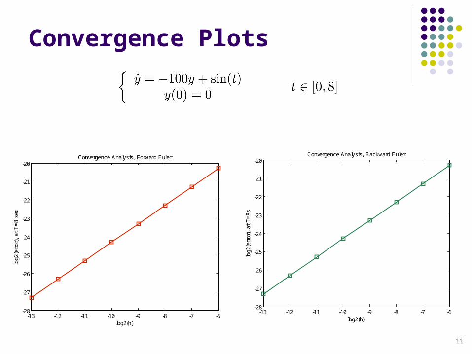
Convergence Plots

11

-13 -12 -11 -10 -9 -8 -7 -6-28

-27

-26

-25

-24

-23

-22

-21

-20Convergence Analysis, Forward Euler

log2(h)

log2

(err

or),

at

T=

8 se

c

-13 -12 -11 -10 -9 -8 -7 -6-28

-27

-26

-25

-24

-23

-22

-21

-20Convergence Analysis, Backward Euler

log2(h)

log2

(err

or),

at

T=

8s

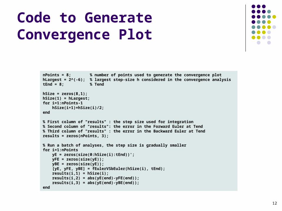
Code to Generate Convergence Plot

12

nPoints = 8; % number of points used to generate the convergence plothLargest = 2^(-6); % largest step-size h considered in the convergence analysistEnd = 8; % Tend

hSize = zeros(8,1);hSize(1) = hLargest;for i=1:nPoints-1 hSize(i+1)=hSize(i)/2;end

% First column of "results" : the step size used for integration% Second column of "results": the error in the Forward Euler at Tend% Third column of "results" : the error in the Backward Euler at Tendresults = zeros(nPoints, 3);

% Run a batch of analyses, the step size is gradually smallerfor i=1:nPoints yE = zeros(size(0:hSize(i):tEnd))'; yFE = zeros(size(yE)); yBE = zeros(size(yE)); [yE, yFE, yBE] = fEulerVSbEuler(hSize(i), tEnd); results(i,1) = hSize(i); results(i,2) = abs(yE(end)-yFE(end)); results(i,3) = abs(yE(end)-yBE(end));end

Implicit Methods, The Ugly Part

Why not always use implicit integration methods?

Implicit method come with some baggage: you need to solve an equation (or system of equations) at *each* integration time step tn

Specifically, look at Backward Euler. At each tn, you need to solve for yn. This is a nonlinear equation, since f(t,y) in general is a nonlinear function

Solving nonlinear systems is something that I’d avoid if possible…

13

Implicit Integration, Solving the Nonlinear System

Note that if you are dealing with a system of ODEs, that is, if y is a vector quantity, you have to solve not a nonlinear equation, but a nonlinear system of equations:

14

We’ll assume in what follows (as almost always the case) that the system above is a nonlinear one Issues that we discuss in this context:

The “functional iteration” approach to finding yn

Newton Iteration

Approximating the Jacobian associated with the nonlinear system

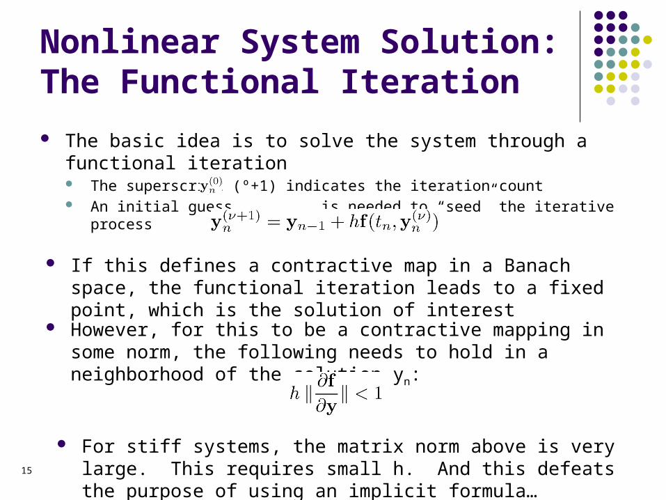
Nonlinear System Solution: The Functional Iteration

The basic idea is to solve the system through a functional iteration The superscript (º+1) indicates the iteration count An initial guess is needed to “seed” the iterative process

15

If this defines a contractive map in a Banach space, the functional iteration leads to a fixed point, which is the solution of interest

However, for this to be a contractive mapping in some norm, the following needs to hold in a neighborhood of the solution yn:

For stiff systems, the matrix norm above is very large. This requires small h. And this defeats the purpose of using an implicit formula…

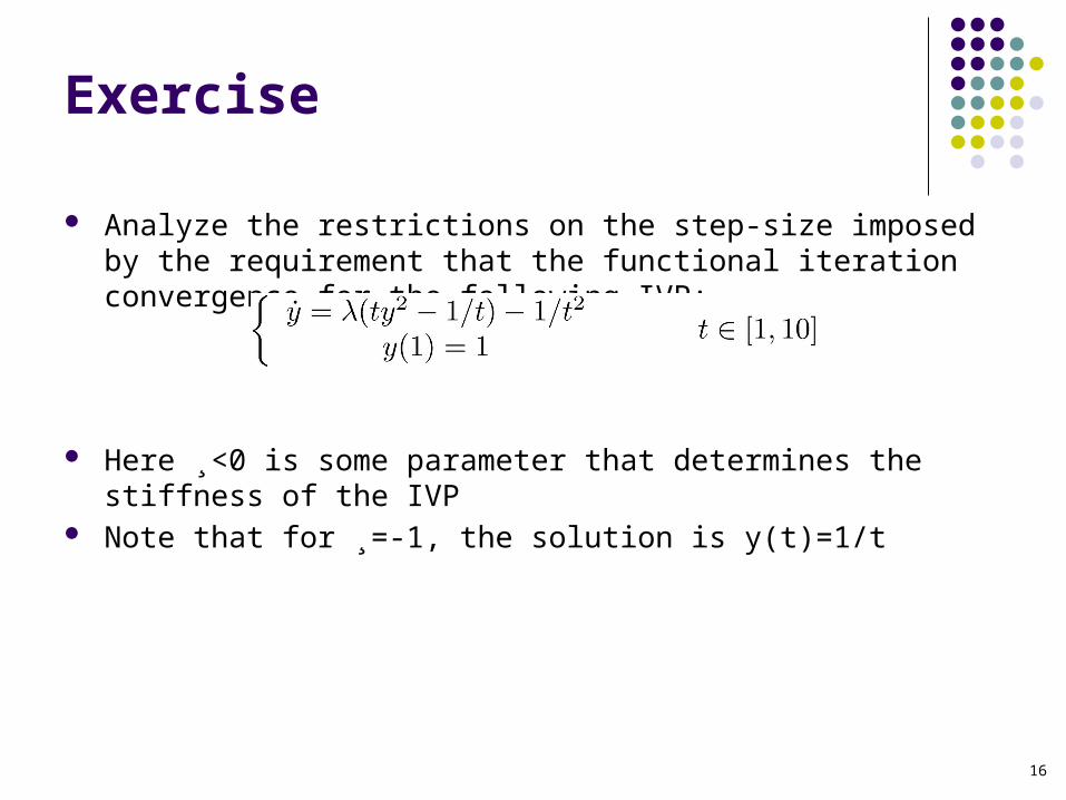
Exercise

Analyze the restrictions on the step-size imposed by the requirement that the functional iteration convergence for the following IVP:

16

Here ¸<0 is some parameter that determines the stiffness of the IVP Note that for ¸=-1, the solution is y(t)=1/t

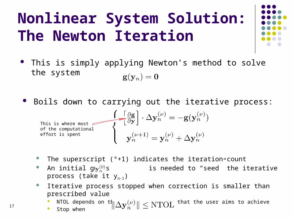
Nonlinear System Solution: The Newton Iteration

The superscript (º+1) indicates the iteration count An initial guess is needed to “seed” the iterative process (take it yn-1) Iterative process stopped when correction is smaller than prescribed value

NTOL depends on the local error bound that the user aims to achieve Stop when

17

This is simply applying Newton’s method to solve the system

Boils down to carrying out the iterative process:

This is where most of the computationaleffort is spent

Nonlinear System Solution: The Newton Iteration

18

Iteration matrix:

Note that the iteration matrix is guaranteed to be nonsingular for small enough values of the step-size h

The iteration matrix is not updated at each iteration. Updated only when convergence in Newton iteration gets poor

Note that each update also requires LU factorization of iteration matrix Adding insult to injury…

Typically, the approach does not place harsh limits on the value of the step size

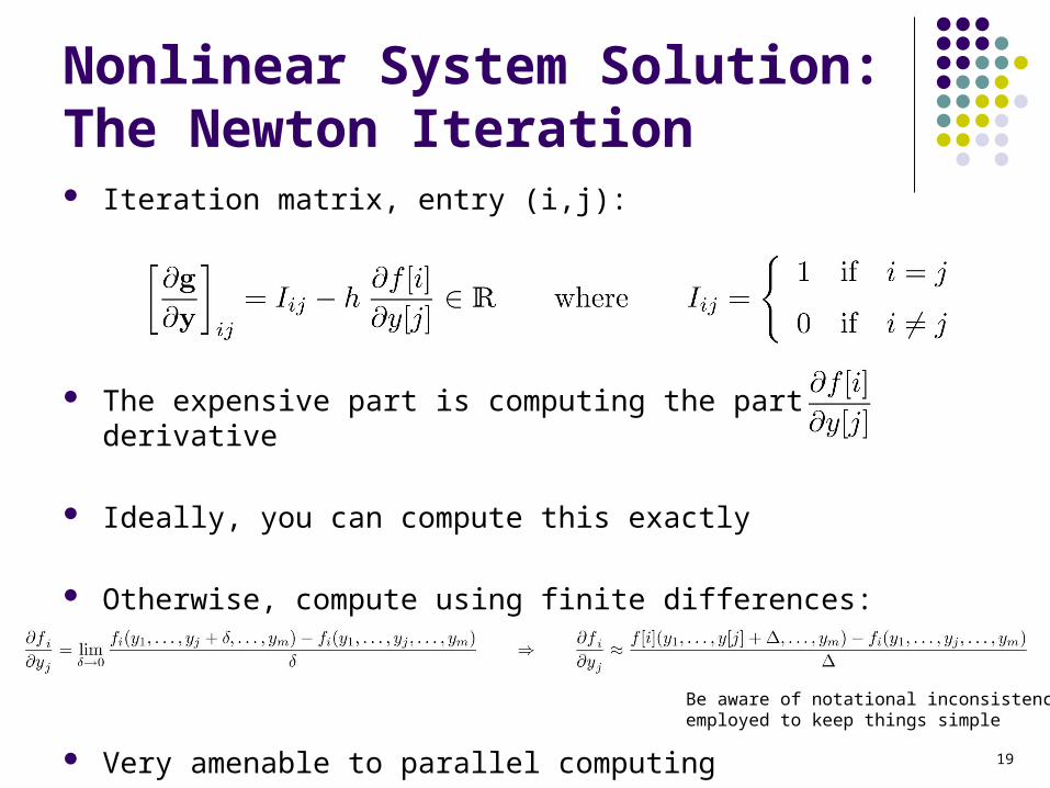
Nonlinear System Solution: The Newton Iteration

19

The expensive part is computing the partial derivative

Ideally, you can compute this exactly

Otherwise, compute using finite differences:

Very amenable to parallel computing

Iteration matrix, entry (i,j):

Be aware of notational inconsistency; employed to keep things simple

Exercise[AO, Handout]

For IVP below, find iteration matrix when solved with B. Euler Find it analytically Find it using finite differences In both cases use for evaluating the matrix

20

[Stability, First Flavor]

A-Stable Integration Methods

Definition, A-Stability First, recall the region of absolute stability: defined in conjunction with

the test IVP, represents the region where h¸ should land so that

By definition, a numerical integration scheme is said to be A-stable if its region of absolute stability covers the entire left half-plane Forward Euler is not A-stable Backward Euler is A-stable

21

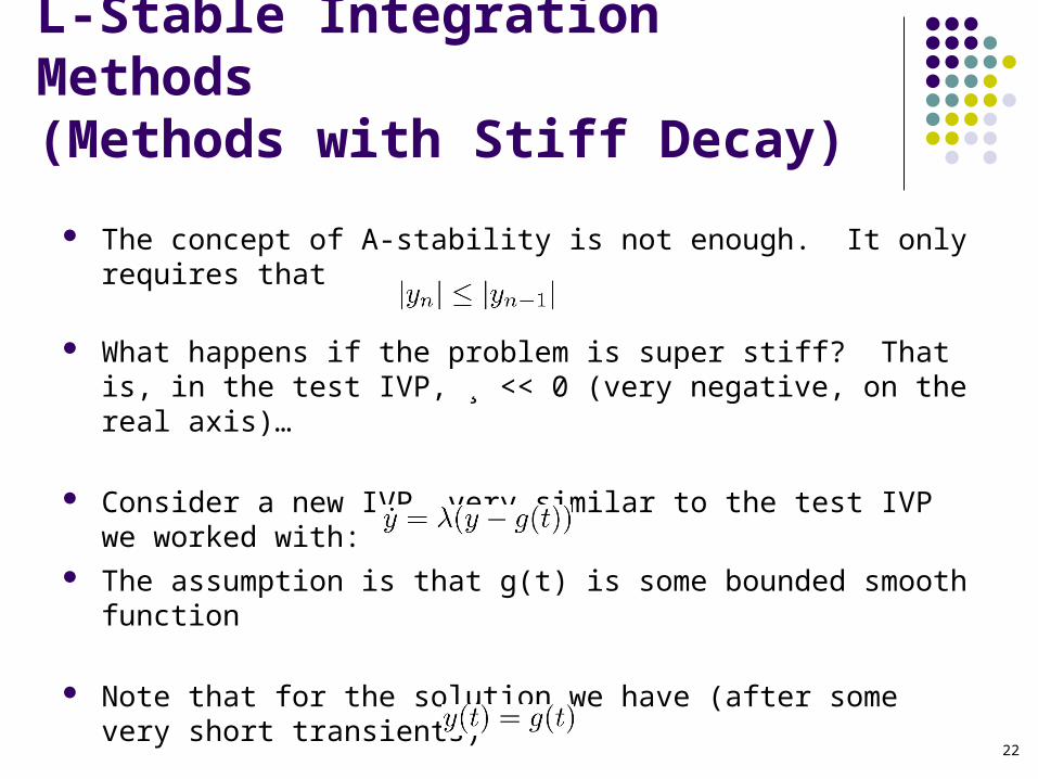
The concept of A-stability is not enough. It only requires that

22

What happens if the problem is super stiff? That is, in the test IVP, ¸ << 0 (very negative, on the real axis)…

Consider a new IVP, very similar to the test IVP we worked with:

The assumption is that g(t) is some bounded smooth function

Note that for the solution we have (after some very short transients)

[Stability, Second Flavor]

L-Stable Integration Methods(Methods with Stiff Decay)

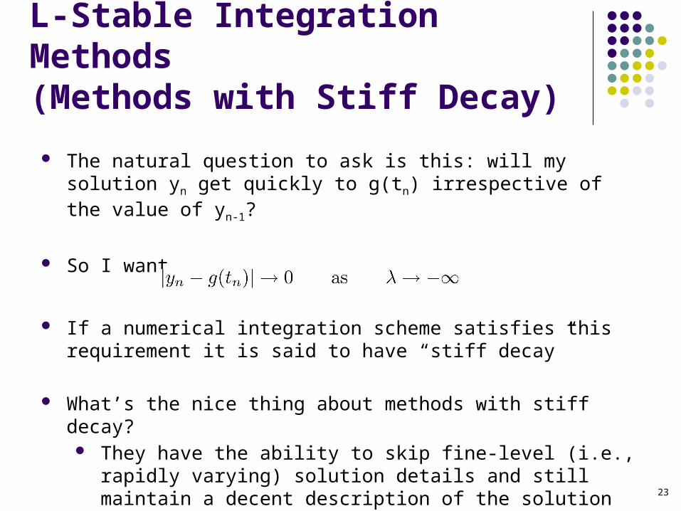
The natural question to ask is this: will my solution yn get quickly to g(tn) irrespective of the value of yn-1?

So I want

23

If a numerical integration scheme satisfies this requirement it is said to have “stiff decay”

What’s the nice thing about methods with stiff decay? They have the ability to skip fine-level (i.e., rapidly varying)

solution details and still maintain a decent description of the solution on a coarse level in the very stiff case

[Stability, Second Flavor]

L-Stable Integration Methods(Methods with Stiff Decay)

Prove that Forward Euler doesn’t have stiff decay Prove that Backward Euler has stiff decay Does the trapezoidal formula (provided below) have stiff decay?

Plot the numerical solution of the following IVP, first obtained with Backward Euler and then with the trapezoidal formula. Comment on the relevance of the stiff decay attribute:

24

Exercise

Further Exercises

Out of Ascher & Petzold book:

Problem 3.1 Problem 3.2 Problem 3.3 Problem 3.9

25

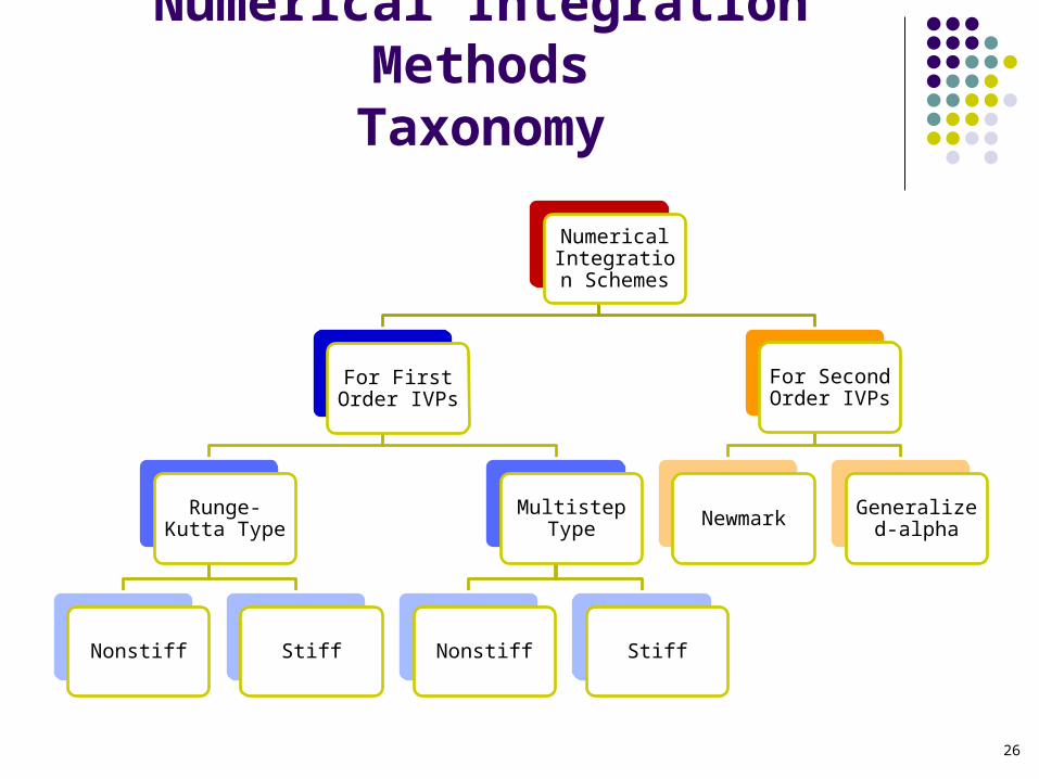
Numerical Integration MethodsTaxonomy

Numerical Integration Schemes

For First Order IVPs

Runge-Kutta Type

Nonstiff Stiff

Multistep Type

Nonstiff Stiff

For Second Order IVPs

Newmark Generalized-alpha

26