mcs lecutre05
DESCRIPTION
boohoo.TRANSCRIPT

Modern Control Systems 1
Lecture 05 Analysis (I)Time Response and State Transition Matrix
5.1 State Transition Matrix
5.2 Modal decomposition --Diagonalization
5.3 Cayley-Hamilton Theorem

Modern Control Systems 2
)()()(
)()()(
tDutCxty
tButAxtxdt
d
1. Homogeneous solution of x(t) 2. Non-homogeneous solution of x(t)
The behavior of x(t) et y(t) :

Modern Control Systems 3
Homogeneous solution
)0()()(
)()0()(
)()(
1 xAsIsX
sAXxssX
tAxtx
)0(
)0(])[()( 11
xe
xAsILtxAt
])[()( 11
AsILet At
State transition matrix
)()()()()(
)()0(
)0()(
000)(
0
0
0
00
0
0
txtttxetxeetx
txex
xetx
ttAAtAt
At
At

Modern Control Systems 4
Properties
)()(.5
)()()(.4
)()()0(.3
)()(.2
)0(.1
020112
1
ktt
tttttt
txtx
tt
I
k
])[()( 11
AsILet At

Modern Control Systems 5
Non-homogeneous solution
)()()(
)()()(
tDutCxty
tButAxtxdt
d
tdButxttx
sBUAsILxAsILtx
sBUAsIxAsIsX
sBUxsXAsI
sBUsAXxssX
0
1111
11
)()()0()()(
)]()[()0(])[()(
)()()0()()(
)()0()()(
)()()0()(
Convolution
Homogeneous

Modern Control Systems 6
)()()()()()(
)()()()()(
)()()0()()(
0
0
00
00
0
tDudButCtxttCty
dButtxtttx
dButxttx
t
t
t
t
t
Zero-input response Zero-state response
Modern Control Systems 7
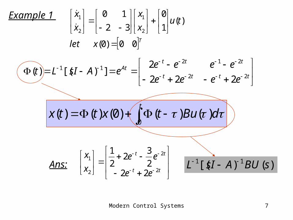
Example 1
Txlet
tux
x
x
x
00)0(
)(1
0
32
10
2
1
2
1
tttt
tttAt
eeee
eeeeeAsILt
22
21211
222
2])[()(
t
dButxttx0
)()()0()()(
tt
tt
ee
eex
x
2
2
2
1
222
32
2
1
Ans: )]()[( 11 sBUAsIL

Modern Control Systems 8
Txlet
tux
x
x
x
00)0(
)(1
0
32
10
2
1
2
1
1s 1s1 1
32
u y1x2x
s
x )0(2
s
x )0(1
Using Maison’s gain formula
)()0()0(2
)(
)()0()0()31(
)(
231
1
2
1
1
2
2
2
2
2
1
11
1
21
sUs
xs
xs
sx
sUs
xs
xss
sx
ss

Modern Control Systems 9
How to find
])[()( 11
AsILet At
State transition matrix
Methode 1: ])[()( 11 AsILt
Methode 3: Cayley-Hamilton Theorem
Methode 2: Atet )(

Modern Control Systems 10
Methode 1: ])[()( 11 AsILt
3
2
1
2
1
2
1
3
2
1
3
2
1
1
0
0
0
0
1
)(
)(
10
01
00
211
340
010
x
x
x
ty
ty
u
u
x
x
x
x
x
x
ssss
ss
sss
ssss
AsI
AsIadjAsI
414
323
32116
33)2)(4(
1
)()(
2
2
2
1

Modern Control Systems 11
Method 2: Diagonalization
3
2
1
3
2
1
3
2
1
166
1
1
1
300
020
001
x
x
x
y
u
x
x
x
x
x
x
t
t
t
At
e
e
e
etΦ3
2
00
00
00
)(
diagonal matrixExample 4.5

Modern Control Systems 12
Eigenvalue of A:
nnRA
][ 21 n,v, , vvT Coordinate transformation matrix
n,v, , vv 21 are independent.
,n,ivAv iiii 1 , satisfying ,
Then eigenvectors,
n 321Assume that all the eigenvalues of A are distinct, i.e.
Diagonalization via Coordinate Transformation
DuCxy
BuAxx
Plant:
matrix. diagonala is 1ATTΛ

Modern Control Systems 13
n
ATT
0
0
2
1
1
1 TTee ΛtAt
t
t
t
Λt
ne
e
e
e
λ0
02
1
where

Modern Control Systems 14
nnn
2
1
2
1
2
1
00
0
000
000
,)0()0()0()()( 221121
nt
ntt ξevξevξevtTtx n
Hence, system asy. stable ⇔ all the eigenvales of A lie in LHP
)0()0( 1xTξ
ATT 1
,n,itt iii 1 ),()(
New coordinate:
Solution of (4.1):
(4.1)
,n,iet it
ii 1 (0),)(
xTξ -1
CTC
BTB
ATTA
1
1
The above expansion of x(t) is called modal decomposition.

Modern Control Systems 15
2
1)0( ,
21
12xxx 3,1 21
11
1121 vvT
11
11
2
11T
xTξ 1
Example
1
10
211
121)(
21
11
21
1111 v
v
v
vvAI
1
10
231
123)(
2
1
22
1222 v
v
v
vvAI
30
011ATT
Find eigenvector
distincti

Modern Control Systems 16
ξξ
30
01
22
11
3
1
)0(
)0()0( ),0()0(
2
11
xT
)0()0()()( 221121 ξevξevtTξtx tt
2
12
3
)0()0()0( 1 ξxTξ
1
1
2
1
1
1
2
3)( 3tt eetx
tt
tt
ee
ee
3
3
2
1
2
32
1
2
3
Solution of (4.1):
(4.2)

Modern Control Systems 17
n 321
In the case of A matrix is phase-variable form and
112
11
2121
111
nn
nn
nnvvvP
Vandermonde matrixfor phase-variable form
4
3
2
1
1
APP
1 PPee tAt

Modern Control Systems 18
Example: distincti
)2)(1)(1(
200
010
101
200
010
101
AIA
0
100
000
100
)(
3
2
1
11
v
v
v
VAI21
depend
0
1
0
000
0
0
1
000
3
2
1
321
3
2
1
321
v
v
v
vvv
v
v
v
vvv
21 VV
distinctnot is i.e. case, eigenvalue Repeated i

Modern Control Systems 19
0
000
010
101
)(
3
2
1
33
v
v
v
VAI23
1
0
1
00
3
2
1
321
v
v
v
vvv
200
010
001
100
010
1011
321 APPVVVP

Modern Control Systems 20
Case 3: distincti Jordan form
321
formJordanAPPvvvP 1321
Generalized eigenvectors
231
121
11
)(
)(
0)(
vvAI
vvAI
vAI
1
1
11 1
1ˆ
AAPP
t
tt
tttt
tA
e
tee
etee
e1
11
12
11
2ˆ

Modern Control Systems 21
Example:
2)2(11
13
11
13
A
1
10
11
11)(
12
11
12
1111 v
v
v
vVAI
0
1
1
1
11
11)(
22
21
22
2121 v
v
v
vVAI
20
12ˆ01
11 121 AAPPVVP
1ˆ
2
22ˆ
PPee
e
teee tAAt
t
tttA

Modern Control Systems 22
Method 3: Cayley-Hamilton Theorem
Theorem: Every square matrix satisfies its char. equation.
0)( 011
1 aaaf n
nn
0)( 011
1 IaAaAaAAf n
nn
Given a square matrix A, . Let f(λ) be the char. polynomial of A.
Char. Equation:
By Caley-Hamilton Theorem
nnRA

Modern Control Systems 23
AaAaIaAaAaa
AaAaAaA
IaAaAaA
IaAaAaA
nnn
nn
n
nn
n
nn
n
02
1011
11
02
111
011
1
011
1
)(
0
nn AkAkAkIkAf 2
210)(any
1
0
11
2210)(
n
k
kk
nn
A
AAAIAf

Modern Control Systems 24
10
21?100 AAExample:
AIAAflet 10100)(
2,1,0)2)(1(20
2121
100210
10022
100110
10011
2)(
1)(
f
f
12
22100
1
1000
10
221
10
21)12(
10
01)22()(
101100100100AAf

Modern Control Systems 25
02
13? AeAtExample:
2,1,02
1321
2)2(
)1(
102102
10110
t
t
ef
eftt
tt
ee
ee
2
1
20 2
tttt
tttt
ttttAt
eeee
eeee
eeeee
222
2
02
13)(
10
012
22
22
22

Modern Control Systems 26

Modern Control Systems 27

Modern Control Systems 28

Modern Control Systems 29

Modern Control Systems 30

Modern Control Systems 31

Modern Control Systems 32
Example:
xy
uxbuAxx
101
0
1
1
102
414
102
1,1,0
0
1
0
,
1
0
1
,
2
4
1
21 vv

Modern Control Systems 33
Example:
xy
uxbuAxx
001
1
0
0
212
100
010