mcmc analysis of classical time series...

MCMC analysis

of classical time series algorithms.

Isambi [email protected]

Lappeenranta University of Technology

Lappeenranta, 19.03.2009

IntroductionTheoretical background

Practical resultsConclusion

Outline

1 Introduction

2 Theoretical backgroundBox-Jenkins modelsBox-Jenkins model identificationBox-Jenkins model estimation

3 Practical resultsSeries generationBox-Jenkins recursive estimationRegression estimation with new noise valuesMatlab garchfit estimation

4 Conclusion

Isambi Sailon MCMC analysis of classical time series algorithms.



The aim of this work is to combine the modern MCMC approachwith classical time series algorithms, to analyse predictivedistributions of estimated parameters.

There are three main phases to be analysed: phase one will be aboutTime Series analysis, phase two will be MCMC series and phasethree will be the MCMC analysis for classical time series.




Box-Jenkins modelsBox-Jenkins model identificationBox-Jenkins model estimation

Box-Jenkins models

Mathematical models used typically for accurate short-termforecasts of ’well-behaved’ data (that shows predictable repetitivecycles and patterns) and find the best fit of a time series to pastvalues of this time series, in order to make forecasts.

A time series is a sequence of observations based on a regular timelybasis, e.g. hourly, daily, monthly, annually, etc. The classical timeseries analysis covers fitting autoregressive (AR) and moving average(MA) models.





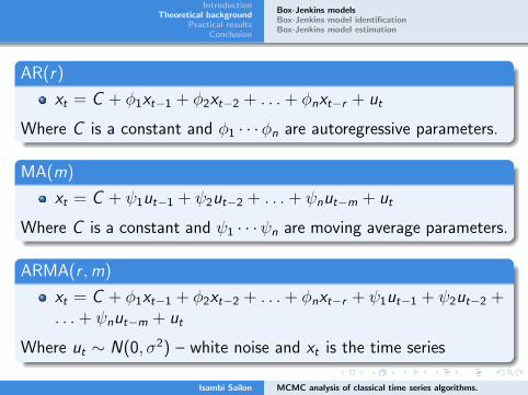
AR(r)

xt = C + φ1xt−1 + φ2xt−2 + . . . + φnxt−r + ut

Where C is a constant and φ1 · · ·φn are autoregressive parameters.

MA(m)

xt = C + ψ1ut−1 + ψ2ut−2 + . . . + ψnut−m + ut

Where C is a constant and ψ1 · · ·ψn are moving average parameters.

ARMA(r ,m)

xt = C + φ1xt−1 + φ2xt−2 + . . . + φnxt−r + ψ1ut−1 + ψ2ut−2 +. . . + ψnut−m + ut

Where ut ∼ N(0, σ2) – white noise and xt is the time series





Autocorrelation (AC)

A certain type of correlation concept that portrays the dependenceof two consecutive observations of time series. ThusAutocorrelations are statistical measures that indicate how a timeseries is related to itself over time.

For example: the autocorrelation at lag 1 is the correlation betweenthe original series and the same series moved forward one period.

rk = E [(xt−µ)(xt+k−µ)]σ2

x

where k is the specified lag number, xt are series observations, µ isthe series mean value and σ2

x is the variance.





The ACF will first test whether adjacent observations areautocorrelated; that is, whether there is correlation betweenobservations 1 and 2, 2 and 3, 3 and 4, etc. This is known as lagone autocorrelation, since one of the pair of tested observations lagsthe other by one period or sample.

Similarly, it will test at other lags. For instance, the autocorrelationat lag four tests whether observations 1 and 5, 2 and 6, ...,19 and23, etc. are correlated.





Estimates at longer lags have been shown to be statisticallyunreliable (Box and Jenkins, 1970). In some cases, the effect ofAutocorrelation at smaller lags will influence the estimate ofautocorrelation at longer lags. For instance, a strong lag oneautocorrelation would cause observation 5 to influence observation6, and observation 6 to influences 7.

This results in an apparent correlation between observations 5 and7, even though no direct correlation exists.





Partial autocorrelation (PAC)

The Partial Autocorrelation Function (PACF) removes the effect ofshorter lag autocorrelation from the correlation estimate at longerlags. PAC is Similar to AC, except that when calculating it, the ACswith all the elements within the lag are partialled out.

rkk =rk−r2

k−1

1−r2k−1

PCA measures the correlation between an observation k periods agoand current observation, after controlling for the observations atintermediate lags (all lags < k), that is, the correlation between yt

and yt−k , after removing the effects of yt−k+1, yt−k+2, · · · , yt−1





Stages in building a Box-Jenkins time series model

1. Model Identification

This involves determining the order of the model required to capturethe dynamic features of the data. Graphical procedures are used todetermine the most appropriate specification (Making sure that thevariables are stationary, identifying seasonality, and the use of plotsof the autocorrelation and partial autocorrelation functions)





2. Model Estimation

This involves estimation of the parameters of the model specified inModel Identification. The most common methods used aremaximum likelihood estimation and non-linear least-squaresestimation, depending on the model.





3. Model Validation

This involves model checking, that is, determining whether themodel specified and estmated is adequate. Thus: Model validationdeals with testing whether the estimated model conforms to thespecifications of a stationary univariate process. It can be done byOverfitting and Residual diagnosis





MODEL IDENTIFICATION

In Box-Jenkins model one has to determine if the series is stationaryand if there is any significant seasonality that needs to be modelled.





A stationary process has the property that the mean, variance andautocorrelation structure do not change over time. It can beassessed by run sequence plot (graph that displays observed data ina time sequence (A graphical data analysis technique for preliminaryscanning of the data).

Also, apart from Run sequence plot, the condition for testingstationarity of AR model is that the roots of the characteristicsequation all lie outside the unit circle.For example xt = 3xt−1 − 2.75xt−2 + 0.75xt−3 + ut is not stationarybecause its roots 1, 2

3and 2 only one lies outside the unit.





xt = 3xt−1 − 2.75xt−2 + 0.75xt−3 + ut is expressed using lagoperator notation thus it will be as follows:xt = 3Lxt − 2.75L2xt + 0.75L3x3 + ut

(1− 3L + 2.75L2 − 0.75L3)xt = ut

The characeristic equation is 1− 3z + 2.75z2 − 0.75z3 = 0. Solvingfor z ; the solution set is 1, 2

3, 2





For seasonality, it means periodic fluctuations, that is, a certainbasic pattern tends to be repeated at regular seasonal intervals.This can be assessed by a run sequence plot, a seasonal subseriesplot, multiple box plots, or autocorrelation plot.





Once stationarity and seasonality have been addressed, one needs toidentify the order (r and m) of the autoregressive and movingaverage terms. The primary tools for doing this are theautocorrelation plot and the partial autocorrelation plot.

The sample autocorrelation plot and the sample partialautocorrelation plot are compared to the theoretical behaviour ofthese plots when the order is known





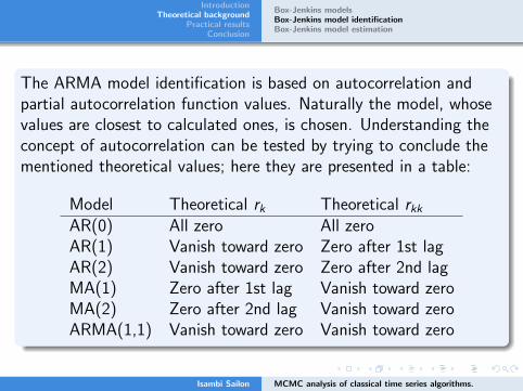
The ARMA model identification is based on autocorrelation andpartial autocorrelation function values. Naturally the model, whosevalues are closest to calculated ones, is chosen. Understanding theconcept of autocorrelation can be tested by trying to conclude thementioned theoretical values; here they are presented in a table:

Model Theoretical rk Theoretical rkkAR(0) All zero All zeroAR(1) Vanish toward zero Zero after 1st lagAR(2) Vanish toward zero Zero after 2nd lagMA(1) Zero after 1st lag Vanish toward zeroMA(2) Zero after 2nd lag Vanish toward zeroARMA(1,1) Vanish toward zero Vanish toward zero





MODEL ESTIMATION

The classical Box-Jenkins model estimation uses a recursivealgorithm. The objective is to minimize the sum of squares of errors.

If we assume for simplicity the ARMA(1,1) model

xt = φxt−1 + ψut−1 + ut

then the algorithm considers all possible values of φ and ψ and for

them minimizes the sum of squarest∑

i=1

u2i .





In particular, assume we have x0, x1, x2, . . . , xt as the observedstationary series. Initially u0 = 0. Then we have:

x1 = φx0 + ψ · 0 + u1 ⇒ u1 = x1 − φx0

x2 = φx1 + ψ · u1 + u2 ⇒ u2 = x2 − φx1 − ψu1

x3 = φx2 + ψ · u2 + u3 ⇒ u3 = x3 − φx2 − ψu2...xn = φxn−1 + ψ · un−1 + un ⇒ un = xn − φxn−1 − ψun−1

The parameters φ and ψ are varied between (-1,1) (since the series

is required to be stationary), and the sumst∑

i=1

u2i are calculated each

time. Then the proper estimates φ and ψ, and the ut noise valuesare those that give the minimal value of the ut sum of squares.




Series generationBox-Jenkins recursive estimationRegression estimation with new noise valuesMatlab garchfit estimation

a) Generate simple series of at least 1000 observations withcoefficients such that the series are stationary.

ARMA(1,0) → xt = θxt−1 + ut

ARMA(1,1) → xt = θxt−1 + ψut−1 + ut

ARMA(2,0) → xt = θ1xt−1 + θ2xt−2 + ut

ARMA(2,1) → xt = θ1xt−1 + θ2xt−2 + ψ1ut−1 + ut

ARMA(2,2) → xt = θ1xt−1 + θ2xt−2 + ψ1ut−1 + ψ2ut−2 + ut





100 200 300 400 500 600 700 800 900 1000

−5

−4

−3

−2

−1

0

1

2

3

4ARMA(1,0) time series with θ=0.7

Figure: Example ARMA(1,0) time series with x0 = 3, θ = 0.7 and whitenoise ut ∼ N(0, 1).





100 200 300 400 500 600 700 800 900 1000

−5

−4

−3

−2

−1

0

1

2

3

4

5

ARMA(2,1) time series with θ1=0.58 , θ

2=−0.4 and ψ=0.6

Figure: Example ARMA(2,1) time series with x0 = 3, x1 = 2.5,θ1 = 0.58, θ2 = −0.4, ψ = 0.6 and white noise ut ∼ N(0, 1).





b) Perform the Box-Jenkins recursive calculation to estimatemodel parameters and compare results with the originallydefined model parameters.





0.5 0.55 0.6 0.65 0.7 0.75 0.8 0.85 0.90

5

10

15

20

25Histogram for θ estimates

Figure: Normalized histogram of θ estimates obtained from Box-Jenkinsrecursive estimation (original θ = 0.7).





0.4 0.5 0.6 0.7 0.80

10

20

30

40

50

Histogram for θ1 estimates

−1 −0.5 00

5

10

15

20

25

30

35

40

45


0.4 0.5 0.6 0.7 0.80

5

10

15

20

25

30

35

40

45Histogram for ψ estimates

Figure: Normalized histogram of θ1, θ2, ψ estimates obtained fromBox-Jenkins recursive estimation (original θ1 = 0.58, θ2 = −0.4,ψ = 0.6).





c) Generate new values for the noise in all models and estimateparameters using regression (backslash operation in Matlab).





0.4 0.45 0.5 0.55 0.6 0.65 0.7 0.75 0.80

2

4

6

8

10

12

14

16

18


Figure: Normalized histogram of θ estimates obtained from regressionestimation (original θ = 0.7).





0.7 0.8 0.9 10

5

10

15

20


−0.8 −0.7 −0.6 −0.5 −0.40

5

10

15

20


−0.5 0 0.50

2

4

6

8

10


Figure: Normalized histogram of θ1, θ2, ψ estimates obtained fromregression estimation (original θ1 = 0.58, θ2 = −0.4, ψ = 0.6).





d) Use Matlab GARCH toolbox (function garchfit.m inparticular) and compare its estimates with the original modelvalues.





0.5 0.55 0.6 0.65 0.7 0.75 0.8 0.85 0.90

2

4

6

8

10

12

14

16

18


Figure: Normalized histogram of θ estimates obtained from Matlabgarchfit.m estimation (original θ = 0.7).





0.4 0.5 0.6 0.7 0.80

2

4

6

8

10

12

14


−1 −0.5 00

2

4

6

8

10

12

14


0.4 0.5 0.6 0.7 0.80

2

4

6

8

10

12


Figure: Normalized histogram of θ1, θ2, ψ estimates obtained fromMatlab garchfit.m estimation (original θ1 = 0.58, θ2 = −0.4, ψ = 0.6).




Recursive Estimation

The recursive estimation gives better results. The multiple runs giveresults that are close to the original parameters values.

New Noise and Regression Estimation

With new noise values used for regression estimation, the results aresignificantly different from the original ones. For instance the resultsshow zero value for ψ while the original ψ was 0.6.

GARCHFIT.M

Using the built in MATLAB function garchfit.m, the results are closeto the original parameter values.




Future work

After this classical time series, the next step is MCMC algorithmswhich will be followed by combining the MCMC analysis with theclassical time series. Here the MCMC will be used to study the timeseries algorithms for parameter prediction (that is the use of formalMCMC to analyse the classical Box-Jenkins parameter estimation).




ASANTENI


mcmc analysis of classical time series...

Documents