MCE693/793: Analysis and

Control of Nonlinear Systems

Systems of Differential EquationsPhase Plane Analysis

Hanz Richter

Mechanical Engineering Department

Cleveland State University

Systems of Nonlinear Differential Equations

2 / 36

We often work with systems in the general form:

x = f(t, x)

where solutions x(t) take values in Rn and f(t, x) is a function defined on a subset of

R× Rn.

Whether the above systems admits one, none or multiple solutions given an initialpoint x(t0) = x0, is a fundamental question.

Can we find a solution tox = − sign (x)?

How aboutx = x1/3?

(from Khalil, Sect. 2.2).We need a few mathematical concepts to answer existence and uniqueness ofsolutions.

Norms in Euclidean Space

3 / 36

The n−dimensional Euclidean space (over the real field) is formed by all vectorsx = [x1, x2, ...xn]

T where xi ∈ R for all i = 1, 2...n.

The norm ||x|| of a vector is a real-valued function satisfying four axioms for allx, y ∈ R

n:

1. ||x|| ≥ 0

2. ||x|| = 0 ⇐⇒ x = 0

3. ||αx|| = |α|||x|| for all α ∈ R

4. ||x+ y|| ≤ ||x||+ ||y||

We are familiar with the Euclidean norm since childhood: ||x|| =√

∑ni=1

x2

i . Butother norms are commonly used.

Show that ||x|| = maxi|x|i is a valid norm.

How to extend the idea of norm to matrices will be discussed later

Continuity and Uniform Continuity of Functions

4 / 36

We consider functions in Euclidean space, f : Rn 7→ Rm. We look at two

equivalent definitions:

1. f is continuous at a point x if the sequence f(xk) converges to f(x) forany sequence xk which converges to x. Succintly, f(xk) → x as xk → x.

2. Given any ǫ > 0, we can find δ(ǫ, x) > 0 such that

||x− y|| < δ(x, ǫ) → ||f(x)− f(y)|| < ǫ

When δ(x, ǫ) is actually independent of x in the second definition, we speak ofuniform continuity.

Important: Uniform continuity obviously implies continuity, but the reverse isalso true when f : S 7→ R

m, where S ⊂ Rn is compact (closed and bounded).

Continuity in Some Variables and Piecewise Continuity

5 / 36

The function f(x, y) = x sign (y)− yx2 is continuous in x but not in y.Specifically, continuity in a subset of variables is evaluated by regarding theremaining variables as constants.The function round(x) for x ∈ R is not continuous, but it ispiecewise-continuous.That is, its domain can be partitioned into regions where the function iscontinuous. In this case, round(x) is continuous on any interval of the form:

(k + 0.5, k + 1.5), k = 0,±1,±2,±3....

Lipschitz Condition, Local Existence and Uniqueness

6 / 36

Theorem (Khalil 2.2) Let f(t, x) be piecewise continuous in t and suppose theLipschitz condition

||f(t, x)− f(t, y)|| ≤ L||x− y||

holds for some constant L > 0, for all x, y in some closed ball of radius rcentered at x0 and for all t in [t, t0]. Then the differential equation

x = f(t, x)

with initial condition x(t0) = x0 has a unique solution in an interval[t0, t0 + δ], for some δ > 0.

Example: for f(x) = −x2, use the above Theorem to analyze existence anduniqueness. Can the solution be continued indefinitely for any initialconditions?

Global Existence and Uniqueness

7 / 36

The previous example shows that solutions may be short-lived unless we placeadditional conditions. The Lipschitz condition will have to hold not onlylocally, but globally in x and in an extended set for t. Boundedness of f(t, x0)will also be required.

Theorem (Khalil 2.3) Let f(t, x) be piecewise continuous in t and suppose theconditions

||f(t, x)− f(t, y)|| ≤ L||x− y||

||f(t, x0)|| ≤ h

hold for all x, y ∈ Rn, all t ∈ [t0, t1] and some h > 0. Then the differential

equationx = f(t, x)

with initial condition x(t0) = x0 has a unique solution in the interval [t0, t1]

Constant Solutions (Equilibrium Points)

8 / 36

Equilibrium points are solutions of the form x(t) = c, for some constant c,valid for all t. They reflect operating setpoints in engineering systems andmust be studied carefully.

Nonlinear systems may have empty, finite or infinite equilibrium sets. The lastclass may consist of a continuum of equilibria or countless isolated points, or amix.

Finding and characterizing the cardinality of equilibrium sets involves thesolution of the nonlinear equations

f(t, x) = 0

We point out that most of the time we use autonomous systems (where t doesnot appear in f), but it is possible to find equilibria in non-autonomoussystems. For example:

x = f(t, x) = cos(t)x

has x = 0 as the single equilibrium point, regardless of t. But the behavior ofthe solution away from zero is influenced by the cos(t) factor.

Examples: Equilibrium Finding

9 / 36

Whenever an analytical solution to f(x) = 0 is not possible, we must usenumerical tools. Matlab’s fsolve is useful.

Find all equilibrium points for the tunnel diode example in Khalil (1.2) andverify the solution provided there using fsolve.

Find all equilibrium points for the second-order system

x = round(y)

y = sin(x)

and sketch them in the phase plane (x-y plane)

Control Systems and Equilibrium

10 / 36

A control system (a system with an exogenous input) includes an additionalargument in f :

x = f(t, x, u)

where u may be specified as a function u(t, x) with values in Rm.

Although is may be possible to find constant solutions when u is non constant(take f(x, u) = cos(u)x, then x = 0 is an equilibrium point regardless of howu varies), the accepted definition of equilibrium points for control systemsinvolves setting u to some constant u0.

It is clear then that the equilibrium solutions depend on u0. Forequilibrium-finding purposes, u0 is simply treated as a parameter of f .

Equilibrium Point Stability

11 / 36

We know that equilibrium solutions are stationary, that is, the system remainsat its initial condition x0 indefinitely whenever x0 is an equilibrium point.

More importantly, we want to determine whether the system has the“tendency” toreturn to x0 if a small initial condition offset is used, or if it moves away from x0.

Stable Unstable

Equilibrium Point Stability

12 / 36

In engineering we normally prefer systems that regulate themselves back totheir original operating point when perturbed. When systems don’t have thatnatural tendency (example: magnetic levitation), we must add feedbackcontrols to change system behavior from unstable to stable.

A precise definition of stability is pending. With Lyapunov’s linearizationmethod, we determine the stability of an equilibrium point of a nonlinearsystem by examining the stability of the linearized system about the origin.

Except for one case (zero eigenvalues), the stability of the linearized system isthe same as the local stability of the nonlinear system.

Review of Small-Signal (Jacobian) Linearization

13 / 36

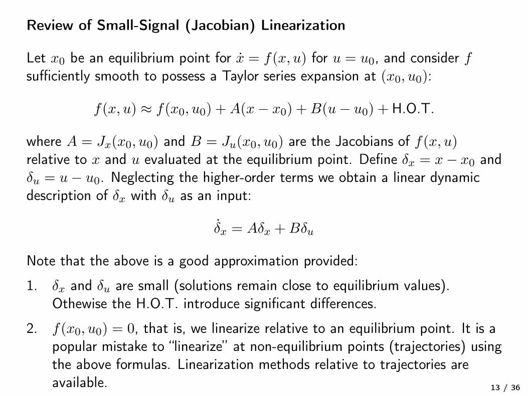
Let x0 be an equilibrium point for x = f(x, u) for u = u0, and consider fsufficiently smooth to possess a Taylor series expansion at (x0, u0):

f(x, u) ≈ f(x0, u0) +A(x− x0) +B(u− u0) + H.O.T.

where A = Jx(x0, u0) and B = Ju(x0, u0) are the Jacobians of f(x, u)relative to x and u evaluated at the equilibrium point. Define δx = x− x0 andδu = u− u0. Neglecting the higher-order terms we obtain a linear dynamicdescription of δx with δu as an input:

δx = Aδx +Bδu

Note that the above is a good approximation provided:

1. δx and δu are small (solutions remain close to equilibrium values).Othewise the H.O.T. introduce significant differences.

2. f(x0, u0) = 0, that is, we linearize relative to an equilibrium point. It is apopular mistake to “linearize” at non-equilibrium points (trajectories) usingthe above formulas. Linearization methods relative to trajectories areavailable.

Equilibria in Linear Systems

14 / 36

Consider the n-state linear system

x = Ax

As we saw before, the equilibrium set is either 0 (when A is nonsingular) ora linear subspace of Rn (when A is singular).

We also know that the system is asymptotically stable whenever all eigenvaluesof A have negative real parts. This implies non-singularity and uniqueness ofequilibrium. If at least one eigenvalue is zero, singularity follows and a denseequilibrium set arises.

Second-order systems are highly relevant and allow graphical study throughphase-plane analysis. In linear systems, we can completely characterizesolution behavior by examining the eigenvalues and eigenvectors of A. In thesecond-order case, graphical representations are very useful.

2nd-Order Linear Systems: Distinct real eigenvalues

15 / 36

When the two eigenvalues are real, distinct and nonzero, twolinearly-independent real eigenvectors v1 and v2 can be found. Then A isdiagonalizable by the transformation x = Tz, with T = [v1 v2]. In z (modal)coordinates, the system becomes decoupled:

z1 = λ1z1

z2 = λ2z2

The solutions are single exponential functions, and satisfy z2 = czλ2/λ1

1 forsome constant c dependent on initial conditions. The signs of λ1 and λ2

determine stability and the shape of the phase portrait.

Stable and Unstable Nodes in Modal Phase Space

16 / 36

If both eigenvalues are negative, we have a stable node. If at least one ispositive, we have an unstable node.

In modal space, eigenvectors are (0,1) and (1,0). Recall that an initialcondition belonging to the span of an eigenvector generates a trajectory alongthe eigenvector.

Stable and Unstable Nodes in Original Phase Space

17 / 36

In phase space, eigenvectors are v1 (slow) and v2 (fast). All solutions are linearcombinations of eigensolutions. Again, an initial condition belonging to thespan of an eigenvector generates a trajectory along the eigenvector.

Saddle Point

18 / 36

If the eigenvalues have opposite signs, the equilibrium point is a saddle.Examine solution behaviors near the stable and unstable eigenvectors.

Straight-Line Solutions

19 / 36

If the eigenvalues are real and one of them is zero, there are straight line

solutions. To see this, note that there is still a set of linearly-independenteigenvectors which diagonalize the system via x = Mz, with M = [v1 v2]. Inthese modal coordinates:

z1 = 0

z2 = λ2z2

The fact that phase trajectories are straight lines is obvious from theseequations. Note that A is singular, so the equilibrium set is dense (the nullspace of A).

Straight-Line Solutions...

20 / 36

If the eigenvalues are real and both of them are zero, A could be the zeromatrix. In this case, there are no trajectories and the entire phase plane ismade up of equilibrium points.

But there are matrices whose nullspace has dimension 1 (nonzero A withλ1 = λ2 = 0). In this case, diagonalization leads to

z1 = z2

z2 = 0

Again, trajectories in modal space are horizontal lines. The direction of thetrajectories depends on the initial condition for z2.

Complex Eigenvalues: Stable Focus Points

21 / 36

When the eigenvalues have the form a± bi with a < 0 and b 6= 0, trajectoriesspiral into the equilibrium point. Clocwkise or counterclockwise?

Complex Eigenvalues: Focus Points

22 / 36

When the eigenvalues have the form a± bi with a > 0 and b 6= 0, trajectoriesspiral out of the equilibrium point. Clockwise or counterclockwise?

Imaginary Axis Eigenvalue(s): Center Points

23 / 36

When the eigenvalues have the form bi with b 6= 0, trajectories are periodic.The phase plane is partitioned by periodic orbits, that is, any two periodicorbits have empty intersection and the union of all periodic orbits is the entireplane.

We will not call these orbits limit cycles, because there are no initial conditionsoutside an orbit which converge to it.

Nonlinear 2nd-Order Systems - Isoclines Method

24 / 36

For nonlinear second-order systems, phase portraits can be generated by:

1. Computer simulation and graphics

2. Analytical solution and elimination of time from solutions

3. Method of isoclines

4. Other methods

Methods 2 and 3 can be used to obtain insightful sketches and induce learning.We will focus on the method of isoclines. Given

x1 = f1(x1, x2)

x2 = f2(x1, x2)

we can show that the slope of phase trajectories is given by dx2

dx1= f2(x1,x2)

f1(x1,x2)

Isoclines Method

25 / 36

To use the isoclines method, find and plot all equilibrium points. Thendetermine the locus of phase space points having particular values of slopethat might be informative, such as ∞,±1 and 0.

Fromdx2dx1

=f2(x1, x2)

f1(x1, x2)

note that the slope at equilibrium points is undefined.

Example: Let f1(x1, x2) = x2 and f2(x1, x2) = x1 + x2. Sketch the phaseportrait. Verify against known characteristics of linear systems.

Analytical Method

26 / 36

In some cases, explicit solutions x1(t) and x2(t) can be found, given an initialpoint (x10, x20). If t can be solved for as a function of x1 (or x2), directsubstitution into x2(t) (or x1(t)) results in an implicit relationship describingthe phase trajectory passing through (x10, x20).

Example: Use the analytical method for the previous example.

Guidelines for Computer-Generated Phase Portraits

27 / 36

1. Take advantage of symmetry (also valid for hand sketching, see S&L2.1.3.)

2. Negative-time solutions: start close to the equilibrium point and computebackwards. Define τ = −t and see what happens to the system relative tothis new time. See Khalil, 1.2.5

3. Use Matlab’s ode45 or stiff methods as appropriate and compute solutionsfor short times.

4. See S&L 2.3 to estimate time spans needed for given trajectory lengths.

Limit Cycles - Background Definitions

28 / 36

Consider the autonomous system

x = f(x)

and let x = φ(x0, t) be a solution with x(0) = x0, assumed valid fort ∈ (−∞,∞). Define:

The positive semiorbit through x0 : γ+(x0) = φ(x0, t) : 0 ≤ t < ∞The negative semiorbit through x0: γ−(x0) = φ(x0, t) : −∞ < t ≤ 0

Limit Cycles - Background Definitions

29 / 36

Definition of limit points and sets:

If there is a sequence of times tn with tn → ∞ as n → ∞ such that thesequence φ(tn, x) → p, we call p a positive limit point of the solution.

If there is a sequence of times tn with tn → −∞ as n → ∞ such thatthe sequence φ(tn, x) → p, we call p a negative limit point of thesolution.

The set of all positive limit points of φ(t, x0) is the positive limit set of thesolution.

The set of all negative limit points of φ(t, x0) is the negative limit set ofthe solution.

Limit Cycles - Background Definitions

30 / 36

Definitions of periodic solutions and closed orbits:

The solution φ(t, x0) is nontrivial periodic if x0 is not an equilibrium pointand there is a constant T > 0 such that φ(t+ T, x0) = φ(x0) for all t ≥ 0.The period is the smallest T that meets the above definition.

If φ(t, x0) is nontrivial periodic, the setx ∈ R

n : x = φ(t, x0) for some t is the periodic orbit or closed orbit

associated with the solution.

Limit Cycles - Definition

31 / 36

(Khalil 7.1) A limit cycle is a closed orbit γ such that γ is the positive limit setof some positive semiorbit γ+(x0) or the negative limit set of some negativesemiorbit γ−(x0), for some x0 /∈ γ.

According to this definition, are linear harmonic oscillator solutions limitcycles? How about nonlinear pendulum oscillations?

The van der Pol Equation and its Limit Cycle

32 / 36

The van der Pol equation

x− µ(1− x2)x+ x = 0

was found by the eponymous Dutch researcher when investigating oscillationsin circuits with vacuum tubes.We can interpret the equation as a mass-spring-damper system with nonlineardamping (which can have positive, negative or zero coefficient according to x).

-4 -3 -2 -1 0 1 2 3x

-3

-2

-1

0

1

2

3

x

van der Pol equation trajectories, µ=0.7

x − µ(1 − x2)x + x = 0

van der Pol Equation

33 / 36

We use the van der Pol equation (µ ≥ 0) for an overview of equilibrium pointsand linearization.We also use it to demonstrate the isoclines method andcomputation of time from trajectories.

1. The origin is the only equilibrium point

2. The eigenvalues of the linearized system matrix A always have positivereal parts for µ > 0.

3. Depending on µ, the origin may be a node or a focus, but always unstablefor µ > 0.

4. Find values of µ to obtain each of the above 2 cases.

Limit Cycles in 2nd-Order Systems: 3 Theorems

34 / 36

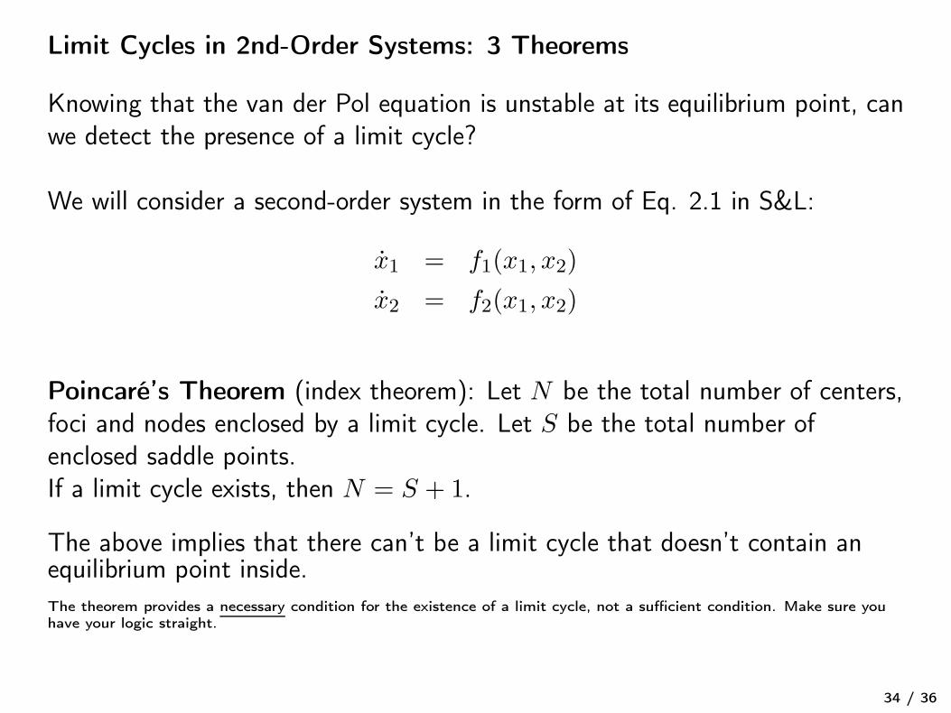
Knowing that the van der Pol equation is unstable at its equilibrium point, canwe detect the presence of a limit cycle?

We will consider a second-order system in the form of Eq. 2.1 in S&L:

x1 = f1(x1, x2)

x2 = f2(x1, x2)

Poincaré’s Theorem (index theorem): Let N be the total number of centers,foci and nodes enclosed by a limit cycle. Let S be the total number ofenclosed saddle points.If a limit cycle exists, then N = S + 1.

The above implies that there can’t be a limit cycle that doesn’t contain anequilibrium point inside.

The theorem provides a necessary condition for the existence of a limit cycle, not a sufficient condition. Make sure youhave your logic straight.

Poincaré-Bendixson Theorem

35 / 36

Statement from S&L:If a trajectory remains in a finite region of the phase plane for all t ≥ 0, thenexactly one of the following holds:

1. The trajectory converges to an equilibrium point

2. The trajectory converges to a limit cycle

3. The trajectory is itself a limit cycle

Examples

Poincaré-Bendixson and Bendixson Theorems

36 / 36

Poincaré-Bendixson:Statement from Khalil:Let γ+ be a bounded positive semiorbit and let L+ be its positive limit set. IfL+ contains no equilibrium points, then it is a periodic orbit.

Bendixson (S&L):If a limit cycle exists in a region Ω of the phase plane, then ∂f1

∂x1+ ∂f2

∂x2must

vanish and change sign somewhere in Ω.

See the interesting proof with Stokes theorem in S&L.Examine the applicability of the three theorems to the van der Pol equation.

Again, we have only a necessary condition. In general, limit cycle detection is a very hard problem. But when they don’texist, ruling them out is immediate using the above theorems.