May-Happen-in-Parallel Analysis forPriority-based Scheduling

Authors’ Version?

Elvira Albert, Samir Genaim, and Enrique Martin-Martin

Complutense University of Madrid, Spain

Abstract. A may-happen-in-parallel (MHP) analysis infers the sets ofpairs of program points that may execute in parallel along a program’sexecution. This is an essential piece of information to detect data races,and also to infer more complex properties of concurrent programs, e.g.,deadlock freeness, termination and resource consumption analyses cangreatly benefit from the MHP relations to increase their accuracy. Previ-ous MHP analyses have assumed a worst case scenario by adopting a sim-plistic (non-deterministic) task scheduler which can select any availabletask. While the results of the analysis for a non-deterministic schedulerare obviously sound, they can lead to an overly pessimistic result. Wepresent an MHP analysis for an asynchronous language with prioritizedtasks buffers. Priority-based scheduling is arguably the most commonscheduling strategy adopted in the implementation of concurrent lan-guages. The challenge is to be able to take task priorities into accountat static analysis time in order to filter out unfeasible MHP pairs.

1 Introduction

In asynchronous programming, programmers divide computations into shortertasks which may create additional tasks to be executed asynchronously. Eachtask is placed into a task-buffer which can execute in parallel with other task-buffers. The use of a synchronization mechanism enables that the execution ofa task is synchronized with the completion of another task. Synchronization canbe performed via shared-memory [9] or via future variables [13, 8]. Concurrentinterleavings in a buffer can occur if, while a task is awaiting for the completion ofanother task, the processor is released such that another pending task can startto execute. This programming model captures the essence of the concurrencymodels in X10 [13], ABS [12], Erlang [1] and Scala [11], and it is the basis of

? Appeared in the Proc. of the 19th International Conference on Logic for Program-ming, Artificial Intelligence, and Reasoning (LPAR-19). Springer, Lecture Notesin Computer Science volume 8312, subline Advanced Research in Computing andSoftware Science (ARCoSS), 2013, pp 18–34. The final publication is available atlink.springer.com.

actor-like concurrency [2, 11]. The most common strategy to schedule tasks isundoubtedly priority-based scheduling. Each task has a priority level such thatwhen the active task executing in the buffer releases the processor, a highestpriority pending task is taken from its buffer and begins executing. Asynchronousprogramming with prioritized tasks buffers has been used to model real-worldasynchronous software, e.g., Windows drivers, engines of modern web browsers,Linux’s work queues, among others (see [9] and its references).

The higher level of abstraction that asynchronous programming provides,when compared to lower-level mechanisms like the use of multi-threading andlocks, allows writing software which is more reliable and more amenable to beanalyzed. In spite of this, proving error-freeness of these programs is still quitechallenging. The difficulties are mostly related to: (1) Tasks interleavings, typ-ically a programmer decomposes a task t into subtasks t1, . . . , tn. Even if eachof the sub-tasks would execute serially, it can happen that a task k unrelatedto this computation interleaves its execution between ti and ti+1. If this taskk changes the shared-memory, it can interfere with the computation in severalways, e.g., leading to non-termination, to an unbounded resource consumption,and to deadlocks. (2) Buffers parallelism, tasks executing across several task-buffers can run in parallel, this could lead to deadlocks and data races.

In this paper, we present a may-happen-in-parallel (MHP) analysis whichidentifies pairs of statements that can execute in parallel and in an interleavedway (see [13, 3]). MHP is a crucial analysis to later prove the properties men-tioned above. It directly allows ensuring absence of data races. Besides, MHPpairs allow us to greatly improve the accuracy of deadlock analysis [16, 10] asit discards unfeasible deadlocks when the instructions involved in a possibledeadlock cycle cannot happen in parallel. Also, it improves the accuracy of ter-mination and cost analysis [5] since it allows discarding unfeasible interleavings.For instance, consider a loop like while (l!=null) {x=b.m(l.data); await

x?; l=l.next;}, where x=b.m(e) posts an asynchronous task m(e) on bufferb, and the instruction await x? synchronizes with the completion of the asyn-chronous task by means of the future variable x. If the asynchronous task is notcompleted (x is not ready), the current task releases the processor and anothertask can take it. This loop terminates provided no instruction that increases thelength of the list l interleaves or executes in parallel with the body of this loop.

Existing MHP analyses [13, 3] assume a worst case scenario by adopting asimplistic (non-deterministic) task scheduler which can select any available task.While the results of the analysis for a non-deterministic scheduler are obviouslysound, they can lead to an overly pessimistic result and report false errors dueto unfeasible schedulings in the task order selection. For instance, consider twobuffers b1 and b2 and assume we are executing a task in b1 with the followingcode “x=b1.m1(e1); y=b1.m2(e2); await x?; b2.m3(e3);”. If the priority ofthe task executing m1 is smaller than that of m2, then it is ensured that taskm2 and m3 will not execute in parallel even if the synchronization via await ison the completion of m1. This is because at the await instruction, when the

2

processor is released, m2 will be selected by the priority-based scheduler beforem1. A non-deterministic scheduler would give this spurious parallelism.

Our starting point is the MHP analysis for non-deterministic scheduling of[3], which distinguishes a local phase in which one inspects the code of each tasklocally, and ignores transitive calls, and a global phase in which the results ofthe local analysis are composed to build a global MHP-graph which captures theparallelism with transitive calls and among multiple task-buffers. The contribu-tion of this paper is an MHP analysis for a priority-based scheduling which takespriorities into account both at the local and global levels of the analysis. As eachbuffer has its own scheduler which is independent of other buffer’s schedulers,priorities can be only applied to establish the order of execution among the tasksexecuting on the same task-buffer (intra-buffer MHP pairs). Interestingly, evenby only using priorities at the intra-buffer level, we are also able to implicitlyeliminate unfeasible inter-buffer MHP pairs. We have implemented our analysisin the MayPar system [4] and evaluated it on some challenging examples, includ-ing some of the benchmarks used in [9]. The system can be used online througha web interface where the benchmarks used are also available.

2 Language

We consider asynchronous programs with priority-levels and multiple tasks bu-ffers. Tasks can be synchronized with the completion of other tasks (of the sameor of a different buffer) using futures. In this model, only highest-priority tasksmay be dispatched, and tasks from different task buffers execute in parallel. Thenumber of task buffers does not have to be known a priori and task buffers canbe dynamically created. We keep the concept of task-buffer disconnected fromphysical entities, such as processes, threads, objects, processors, cores, etc. In [9],particular mappings of task-buffers to such entities in real-world asynchronoussystems are described. Our model captures the essence of the concurrency anddistribution models used in X10 [13] and in actor-languages (including ABS [12],Erlang [1] and Scala [11]). It also has many similarities with [9], the main differ-ence being that the synchronization mechanism is by means of future variables(instead of using the shared-memory for this purpose).

2.1 Syntax

Each program declares a sequence of global variables g0, . . . , gn and a sequenceof methods named m0, . . . ,mi (that may declare local variables) such that oneof the methods, named main, corresponds to the initial method which is neverposted or called and it is executing in a buffer with identifier 0. The grammarbelow describes the syntax of our programs. Here, T are types, m procedurenames, e expressions, x can be global or local variables, buffer identifiers b arelocal variables, f are future variables, and priority levels p are natural numbers.

3

M ::= T m(T x){s; return e; }s ::= s; s | x = e | if e then s else s | while e do s |

await f? | b = newBuffer | f = b.m(〈e〉, p) | release

The notation T is used as a shorthand for T1, ...Tn, and similarly for other names.We use the special buffer identifier this to denote the current buffer. For the sakeof generality, the syntax of expressions is left free and also the set of types is notspecified. We assume that every method ends with a return instruction.

The concurrency model is as follows. Each buffer has a lock that is shared byall tasks that belong to the buffer. Data synchronization is by means of futurevariables as follows. An await y? instruction is used to synchronize with theresult of executing task y=b.m(〈z〉, p) such that await y? is executed only whenthe future variable y is available (and hence the task executing m is finished).In the meantime, the buffer’s lock can be released and some highest prioritypending task on that buffer can take it. The instruction release can be used tounconditionally release the processor so that other pending task can take it.Therefore, our concurrency model is cooperative as processor release points areexplicit in the code, in contrast to a preemptive model in which a higher prioritytask can interrupt the execution of a lower priority task at any point (see Sec. 7).W.l.o.g, we assume that all methods in a program have different names.

2.2 Semantics

A program state St = 〈g, Buf〉 is a mapping g from the global variables to theirvalues along with all created buffers Buf. Buf is of the form buffer1 ‖ . . . ‖ buffern

denoting the parallel execution of the created task-buffers. Each buffer is a termbuffer(bid , lk,Q) where bid is the buffer identifier, lk is the identifier of the activetask that holds the buffer’s lock or ⊥ if the buffer’s lock is free, and Q is theset of tasks in the buffer. Only one task can be active (running) in each bufferand has its lock. All other tasks are pending to be executed, or finished if theyterminated and released the lock. A task is a term tsk(tid ,m, p, l, s) where tidis a unique task identifier, m is the method name executing in the task, p is thetask priority level (the larger the number, the higher the priority), l is a mappingfrom local (possibly future) variables to their values, and s is the sequence ofinstructions to be executed or s = ε(v) if the task has terminated and the returnvalue v is available. Created buffers and tasks never disappear from the state.

The execution of a program starts from an initial state where we have aninitial buffer with identifier 0 executing task 0 of the form S0 = 〈g, buffer(0, 0,{tsk(0,main, p, l, body(main))})〉. Here, g contains initial values for the global vari-ables, l maps parameters to their initial values and local reference and futurevariables to null (standard initialization), p is the priority given to main, andbody(m) refers to the sequence of instructions in the method m. The execu-tion proceeds from S0 by selecting non-deterministically one of the buffers andapplying the semantic rules depicted in Fig. 1. We omit the treatment of thesequential instructions as it is standard, and we also omit the global memory gfrom the state as it is only modified by the sequential instructions.

4

(newbuffer)

fresh(bid ′) , l′ = l[x→ bid ′], t = tsk(tid ,m, p, l, 〈x = newBuffer; s〉)buffer(bid , tid , {t} ∪ Q) ‖ B ;

buffer(bid , tid , {tsk(tid ,m, p, l′, s)} ∪ Q) ‖ buffer(bid ′,⊥, {}) ‖ B

(priority)highestP (Q) = tid , t = tsk(tid , , , , s) ∈ Q, s 6= ε(v)

buffer(bid ,⊥,Q) ‖ B ; buffer(bid , tid ,Q) ‖ B

(async)

l(x) = bid1, fresh(tid1), l′ = l[y → tid1], l1 = buildLocals(z,m1)

buffer(bid , tid , {tsk(tid ,m, p, l, 〈y = x.m1(z, p1); s〉} ∪ Q) ‖ buffer(bid1, ,Q′) ‖ B ;

buffer(bid , tid , {tsk(tid ,m, p, l′, s)} ∪ Q) ‖buffer(bid1, , {tsk(tid1,m1, p1, l1, body(m1))} ∪ Q′) ‖ B

(await1)

l(y) = tid1, tsk(tid1, , , , s1) ∈ Buf, s1 = ε(v)

buffer(bid , tid , {tsk(tid ,m, p, l, 〈await y?; s〉)} ∪ Q) ‖ B ;

buffer(bid , tid , {tsk(tid ,m, p, l, s)} ∪ Q) ‖ B

(await2)

l(y) = tid1, tsk(tid1, , , , s1) ∈ Buf, s1 6= ε(v)

buffer(bid , tid , {tsk(tid ,m, p, l, 〈await y?; s〉)} ∪ Q) ‖ B ;

buffer(bid ,⊥, {tsk(tid ,m, p, l, 〈await y?; s〉)} ∪ Q) ‖ B

(release) buffer(bid , tid , {tsk(tid ,m, p, l, 〈release; s〉)} ∪ Q) ‖ B ;

buffer(bid ,⊥, {tsk(tid ,m, p, l, s)} ∪ Q) ‖ B

(return)

v = l(x)

buffer(bid , tid , {tsk(tid ,m, p, l, 〈return x; 〉)} ∪ Q) ‖ B ;

buffer(bid ,⊥, {tsk(tid ,m, p, l, ε(v))} ∪ Q) ‖ B

Fig. 1. Summarized Semantics for a Priority-based Scheduling Async Language

Newbuffer: an active task tid in buffer bid creates a buffer bid ′ which isintroduced to the state with a free lock. Priority: Function highestP returns ahighest-priority task that is not finished, and it obtains its buffer’s lock. Async:A method call creates a new task (the initial state is created by buildLocals)with a fresh task identifier tid1 which is associated to the corresponding futurevariable y in l′. We have assumed that bid 6= bid1, but the case bid = bid1 isanalogous, the new task tid1 is simply added to Q of bid . Await1: If the futurevariable we are awaiting for points to a finished task, the await can be completed.The finished task t1 is looked up in all buffers in the current state (denoted Buf).Await2: Otherwise, the task yields the lock so that any other task of the samebuffer can take it. Release: the current task frees the lock. Return: When return

5

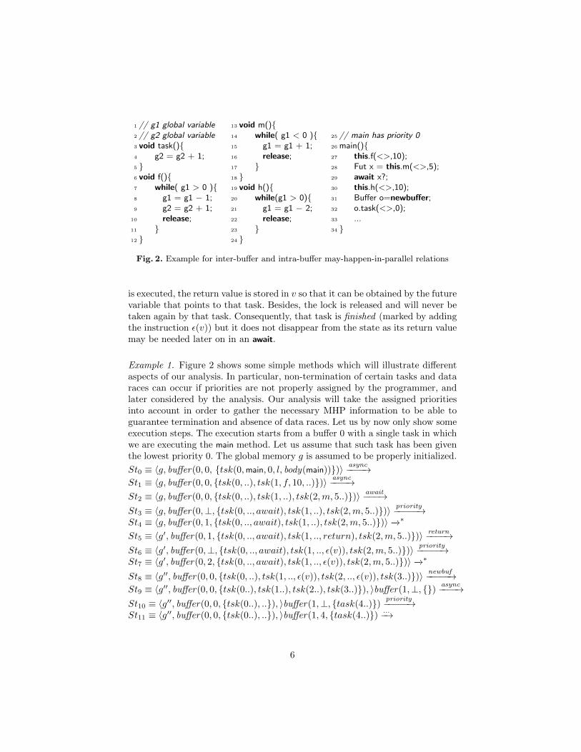
1 // g1 global variable2 // g2 global variable3 void task(){4 g2 = g2 + 1;5 }6 void f(){7 while( g1 > 0 ){8 g1 = g1 − 1;9 g2 = g2 + 1;

10 release;11 }12 }

13 void m(){14 while( g1 < 0 ){15 g1 = g1 + 1;16 release;17 }18 }19 void h(){20 while(g1 > 0){21 g1 = g1 − 2;22 release;23 }24 }

25 // main has priority 026 main(){27 this.f(<>,10);28 Fut x = this.m(<>,5);29 await x?;30 this.h(<>,10);31 Buffer o=newbuffer;32 o.task(<>,0);33 ...34 }

Fig. 2. Example for inter-buffer and intra-buffer may-happen-in-parallel relations

is executed, the return value is stored in v so that it can be obtained by the futurevariable that points to that task. Besides, the lock is released and will never betaken again by that task. Consequently, that task is finished (marked by addingthe instruction ε(v)) but it does not disappear from the state as its return valuemay be needed later on in an await.

Example 1. Figure 2 shows some simple methods which will illustrate differentaspects of our analysis. In particular, non-termination of certain tasks and dataraces can occur if priorities are not properly assigned by the programmer, andlater considered by the analysis. Our analysis will take the assigned prioritiesinto account in order to gather the necessary MHP information to be able toguarantee termination and absence of data races. Let us by now only show someexecution steps. The execution starts from a buffer 0 with a single task in whichwe are executing the main method. Let us assume that such task has been giventhe lowest priority 0. The global memory g is assumed to be properly initialized.

St0 ≡ 〈g, buffer(0, 0, {tsk(0,main, 0, l, body(main))})〉 async−−−−→St1 ≡ 〈g, buffer(0, 0, {tsk(0, ..), tsk(1, f, 10, ..)})〉 async−−−−→St2 ≡ 〈g, buffer(0, 0, {tsk(0, ..), tsk(1, ..), tsk(2,m, 5..)})〉 await−−−→St3 ≡ 〈g, buffer(0,⊥, {tsk(0, .., await), tsk(1, ..), tsk(2,m, 5..)})〉 priority−−−−−→St4 ≡ 〈g, buffer(0, 1, {tsk(0, .., await), tsk(1, ..), tsk(2,m, 5..)})〉 −→∗

St5 ≡ 〈g′, buffer(0, 1, {tsk(0, .., await), tsk(1, .., return), tsk(2,m, 5..)})〉 return−−−−→St6 ≡ 〈g′, buffer(0,⊥, {tsk(0, .., await), tsk(1, .., ε(v)), tsk(2,m, 5..)})〉 priority−−−−−→St7 ≡ 〈g′, buffer(0, 2, {tsk(0, .., await), tsk(1, .., ε(v)), tsk(2,m, 5..)})〉 −→∗

St8 ≡ 〈g′′, buffer(0, 0, {tsk(0, ..), tsk(1, .., ε(v)), tsk(2, .., ε(v)), tsk(3..)})〉 newbuf−−−−−→St9 ≡ 〈g′′, buffer(0, 0, {tsk(0..), tsk(1..), tsk(2..), tsk(3..)}), 〉buffer(1,⊥, {}) async−−−−→St10 ≡ 〈g′′, buffer(0, 0, {tsk(0..), ..}), 〉buffer(1,⊥, {task(4..)}) priority−−−−−→St11 ≡ 〈g′′, buffer(0, 0, {tsk(0..), ..}), 〉buffer(1, 4, {task(4..)}) ...−→

6

At St1, we execute the instruction at Line 27 (L27 for short) that posts, in thecurrent buffer this, a new task (with identifier 1) that will execute method f withpriority 10. The next step St2 posts another task (with identifier 2) in the currentbuffer with a lower priority (namely 5). At St3, an await instruction (L29) is usedto synchronize the execution with the completion of the task 2 spawned at L28.As the task executing f has higher priority than the one executing m, it will beselected for execution at St4. After returning from the execution of task 1 in St5,the priority rule selects task 2 for execution in St6. An interesting aspect isthat after creating buffer 1 at St10, execution can non-deterministically choosebuffer 0 or 1 (in St11 buffer 1 has been selected).

3 Definition of MHP

We first formally define the concrete property “MHP” that we want to approx-imate using static analysis. In what follows, we assume that instructions arelabelled such that it is possible to obtain the corresponding program point iden-tifiers. We also assume that program points are globally different. We use pmto refer to the entry program point of method m, and pm to all program pointsafter its return instruction. The set of all program points of P is denoted by PP .We write p ∈ m to indicate that program point p belongs to method m. Given asequence of instructions s, we use pp(s) to refer to the program point identifierassociated with its first instruction and pp(ε(v)) = pm.

Definition 1 (concrete MHP). Given a program P , its MHP is defined asEP =∪{ES |S0 ∗ S} where for S=〈g, Buf〉, the set ES is ES = {(pp(s1), pp(s2)) |buffer(bid1, ,Q1)∈Buf, buffer(bid2, ,Q2)∈Buf, t1 = tsk(tid1, , , , s1)∈Q1, t2 =tsk(tid2, , , , s2)∈Q2, tid1 6= tid2}.

The above definition considers the union of the pairs obtained from all deriva-tions from S0. This is because execution is non-deterministic in two dimensions:(1) in the selection of the buffer that is chosen for execution, since the buffershave access to the global memory different behaviours (and thus MHP pairs)can be obtained depending on the execution order, and (2) when there is morethan one task with the highest priority, the selection is non-deterministic.

The MHP pairs can originate from direct or indirect task creation relation-ships. For instance, the parallelism between the points of the tasks executing h

and task is indirect because they do not invoke one to the other directly, buta third task main invokes both of them. However, the parallelism between thepoints of the task main and those of task is direct because the first one invokesdirectly the latter one. Def. 1 captures all these forms of parallelism.

Importantly, EP includes both intra-buffer and inter-buffer MHP pairs, eachof which are relevant for different kinds of applications, as we explain below.

7

Intra-buffer MHP pairs. Intra-buffer relations in Def. 1 are pairs in which bid1 ≡bid2. We always have that the first instructions of all tasks which are pendingin the buffer’s queue may-happen-in-parallel among them, and also with theinstruction of the task which is currently active (has the buffer’s lock). Thispiece of information allows approximating the tasks interleavings that we mayhave in a considered buffer. In particular, when the execution is at a processorrelease point, we use the MHP pairs to see the instructions that may executeif the processor is released. Information about task interleavings is essential toinfer termination and resource consumption in any concurrent setting (see [5]).

Example 2. Consider the execution trace in Ex. 1, we have the MHP pairs(29,pf ) and (29,pm) since when the active task 0 is executing the await (point

29) in St4, we have that tasks 1 and 2 are pending at their entry points. Thefollowing execution steps give rise to many other MHP pairs. The most relevantpoint to note is that in St8 when the execution is at L30 and onwards, the tasks1 and 2 are guaranteed to be at their exit program points pf and pm. Thus,we will not have any MHP pair between the instructions that update the globalvariable g1 (L8 and L15 in tasks 1 and 2, resp.) and the release point at L22of the task 3 executing h. This information is essential to prove the terminationof h, as the analysis needs to be sure that the loop counter cannot be modifiedby instructions of other tasks that may execute in parallel with the body of thisloop. The information is also needed to obtain an upper bound on the numberof iterations of the loop and then infer the resource consumption of h.

Inter-buffer MHP pairs. In addition to intra-buffer MHP relations, inter-bufferMHP pairs happen when bid1 6= bid2. In this case, we obtain the instructionsthat may execute in parallel in different buffers. This information is relevantat least for two purposes: (1) to detect data-races in the access to the globalmemory and (2) to detect deadlocks and livelocks when one buffer is awaitingfor the completion of one task running in another buffer, while such other taskis awaiting for the completion of the current task, and the execution of these(synchronization) instructions happens in parallel (or simultaneously). If thelanguage allows blocking the execution of the buffer such that no other pendingtask can take it, we have a deadlock, otherwise we have a livelock.

Example 3. Consider again the execution trace in Ex. 1, in St10 we have createda new buffer 1 in which task 4 starts to execute at St11. We will have the inter-buffer pair (21,4) as we can have L21 executing in buffer 0 and L4 executingin buffer 1. Note that, if task had updated g1 instead of updating g2, we wouldhave had a data race. Data races can lead to different types of errors, and staticanalyses that detect them are of utmost importance.

4 Method-Level Analysis with Priorities

In this section, we present the local phase of our MHP analysis which assignsto each program point, of a given method, an abstract state that describes the

8

(1) τp(y=this.m(x, p),M) = M [〈y,O, Z,R〉/〈?,O, Z,R〉] ∪ {〈y, t, m, p〉}(2) τp(y=x.m(x, p),M) = M [〈y,O, Z,R〉/〈?,O, Z,R〉] ∪ {〈y, o, m, p〉}(3) τp(release,M) = τp(release1; release2,M)(4) τp(release1,M) = M [〈Y, t, m, p〉/〈Y, t, m, p〉] where p ≥ p

(5) τp(release2,M) = M [〈Y, t, m, p〉/〈Y, t, m, p〉] where p > p

(6) τp(await y?,M) = M ′[〈y,O, m,R〉/〈y,O, m,R〉]where M ′ = τp(release1; release2,M)

(7) τp(return,M) = M [〈Y, t, m, R〉/〈Y, t, m, R〉](8) τp(b,M) = M otherwise

Fig. 3. Method-level MHP transfer function: τp : s× B 7→ B.

status of the tasks that have been locally invoked so far. The status of a taskcan be (1) pending, i.e., it is at the entry program point; (2) finished, i.e., it hasexecuted a return instruction already; or (3) active, i.e., it can be executing atany program point (including the entry and the exit). The analysis uses MHPatoms which are syntactic objects of the form 〈F,O, T,R〉 where

– F is either a valid future variable name or ?. The value ? indicates that thetask might not be associated with any future variable, either because there isno need to synchronize with its result, or because the future has been reusedand thus the association lost (this does not happen in our example);

– O is the buffer name that can be t or o, which resp. indicate that the taskis executing on the same buffer or maybe on a different one;

– T can be m, m, or m where m is a method name. It indicates that thecorresponding task is an instance of method m, and its status can be pending,active, or finished resp.;

– P is a natural number indicating the priority of the corresponding task.

Intuitively, an MHP atom 〈F,O, T,R〉 is read as follows: task T might be exe-cuting (in some status) on buffer O with priority P , and one can wait for it tofinish using future variable F . The set of all MHP atoms is denoted by A.

Example 4. The MHP atom 〈x, t, m, 5〉 indicates that there is an instance ofmethod m running in parallel, in the same buffer. This task is active (i.e., canbe at any program point), has priority 5, and is associated with the future x.

The MHP atom 〈?, o, ˆtask, 0〉 indicates that there is an instance of method taskrunning in parallel, maybe in a different buffer. This task is finished (i.e., hasexecuted return), has priority 0, and it is associated to any future variable.

An abstract state is a multiset of MHP atoms from A. The set of all multisetsover A is denoted by B. Given M ∈ B, we write (a, i) ∈ M to indicate that aappears exactly i > 0 times in M . We omit i when it is 1. The local analysisis applied on each method and, as a result, it assigns an abstract state fromB to each program point in the program. The analysis takes into account thepriority of the method being analyzed. Thus, since a method might be called withdifferent priorities p1, . . . , pn, the analysis should be repeated for each pi. For

9

the sake of simplifying the presentation, we assume that each method is alwayscalled with the same priority. Handling several priorities is a context-sensitiveanalysis problem that can be done by, e.g., cloning the corresponding code.

The analysis of a given method, with respect to priority p, abstractly executesits code over abstract elements from B. This execution uses a transfer functionτp, depicted in Fig. 3, to rewrite abstract states. Given an instruction b and anabstract state M ∈ B, τp(b,M) computes a new abstract state that results fromabstractly executing b in state M . Note that the subscript p in τp is the priorityof the method being analyzed. Let us explain the different cases of τp:

– (1) Posting a task on the same buffer adds a new MHP atom 〈y, t, m, p〉to the abstract state. It indicates that an instance of m is pending, withpriority p, on the same buffer as the analyzed method, and is associatedwith future variable y. In addition, since y is assigned a new value, thoseatoms in M that were associated with y should now be associated with ?in the new state. This is done by M [〈y,O, Z,R〉/〈?,O, Z,R〉] which replaceseach atom that matches 〈y,O, Z,R〉 in M by 〈?,O, Z,R〉;

– (2) It is similar to (1), the difference is that the new task might be posted ona buffer different from that of the method being analyzed. Thus, its statusshould be active since, unlike (1), it might start to execute immediately;

– (3)-(5) These cases highlight the use of priorities, and thus mark the maindifferences wrt [3]. They state that when releasing the processor, only tasksof equal or higher priorities are allowed to become active (simulated throughrelease1). Moreover, when taking the control back, any task with strictlyhigher priority is guaranteed to have been finished (simulated through release2).Importantly, the abstract element after release1 is associated to the programpoint of the release instruction, and that after release2 is associated to theprogram point after the release instruction. These two auxiliary instructionsare introduced to simulate the implicit “loop” (in the semantics) when thetask is waiting at that point;

– (6) This instruction is similar to release, the only difference is that the statusof the tasks that are associated with future variable y become finished in thefollowing program point. Importantly, the abstract element after release1 isassociated to the program point of the await y?;

– (7) It changes the status of every pending task executing on the same bufferto active, this is because the processor is released. Note that we do notconsider priorities in this case, since the task is finished.

In addition to using the transfer function for abstractly executing basic instruc-tions, the analysis merges the results of paths (in conditions, loops, etc) using ajoin operator. We refer to [3] for formal definitions of the basic abstract interpre-tations operators. In what follows, we assume that the result of the local phaseis given by means of a mapping L

P:PP 7→B which maps each program point p

(including entry and exit points) to an abstract state LP

(p) ∈ B.

Example 5. Applying the local analysis on main, results in the following abstractstates (initially the abstract state is ∅):

10

28:{〈?, t, f, 10〉}29:{〈?, t, f, 10〉, 〈x, t, m, 5〉}30:{〈?, t, f, 10〉, 〈x, t, m, 5〉}31:{〈?, t, f, 10〉, 〈x, t, m, 5〉, 〈?, t, h, 10〉}32:{〈?, t, f, 10〉, 〈x, t, m, 5〉, 〈?, t, h, 10〉}33:{〈?, t, f, 10〉, 〈x, t, m, 5〉, 〈?, t, h, 10〉, 〈?, o, ˜task, 0〉}

Note that in the abstract state at program point 30 we have both f and m finished,this is because they have higher priority than main, and thus, while main is waitingat program point 29 both f and m must have completed their execution beforemain can proceed to the next instruction. If we ignore priorities, then we wouldinfer that f might be active at program point 30 (which is less precise).

5 MHP Graph for Priority-based Scheduling

In this section we will construct a MHP graph relating program points andmethods in the program, that will be used to extract precise information onwhich program points might globally run in parallel. In order to build this graph,we use the local information computed in Sec. 4 which already takes prioritiesinto account. In Sec. 5.2, we explain how to use the MHP graph to infer theMHP pairs in the program. Finally, in Sec. 5.3 we compare the inference methodof MHP pairs using a priority-based scheduling with the technique introducedin [3] for programs with a non-deterministic scheduling.

5.1 Construction of the MHP Graph with Priorities

The MHP graph has different types of nodes and different types of edges. Thereare nodes that represent the status of methods (active, pending or finished) andnodes that represent the program points. Outgoing edges from method nodesare unweighted and unlabeled, they represent points of which at most one mightbe executing. Outgoing edges from program point nodes are labeled, written →l

where the label l is a tuple (O,R) that contains a priority R and a buffer nameO. These edges represent tasks such that any of them might be running. Besides,when two nodes are directly connected by i > 1 edges, we connect them witha single edge superscripted with weight i, written as →i

l where l is the label asbefore.

Definition 2 (MHP graph with priorities). Given a program P , and itsmethod-level MHP analysis result L

P, the MHP graph of P is a directed graph

GP

= 〈V,E〉 with a set of nodes V and a set of edges E = E1 ∪ E2 defined:

V = {m, m, m | m ∈ PM} ∪ PP

E1 = {m→ p | m ∈ PM , p ∈ PP , p ∈ m} ∪ {m→ pm, m→ pm | m ∈ PM}E2 = {p→i

(O,R) x | p ∈ PP , (〈 , O, x,R〉, i) ∈ LP (p)}

11

˜main

ˇmain ˆmain

292827p ˚main 30 31 33 p ˙main

fff m m m h hh ˜task

8 9 10 15 16 21 22 4

10 105

10

5

10

5

10

10

5

10

0

10

5

10

0

Fig. 4. MHP graph with priorities of the example

Example 6. Fig. 4 depicts the relevant fragment of the MHP graph for our run-ning example. The graph only shows selected program points, namely all pointsof the main task and those points of the other tasks in which there is a release

instruction, or in which the global memory is updated. For each task, we havethree nodes which correspond to their possible status (except for h and task thatwe have omitted status that do not have incoming edges). In order to avoid clut-tering the graph, in edges from program points, the labels only show the priority.The weight is omitted as it is always 1. The label corresponding to the buffername is depicted using different types of arrows: normal arrows correspond tothe buffer name o, while dashed arrows to t. From the pending (resp. finished)nodes, we always have an edge to the task entry (resp. exit) point. From theactive nodes, we have edges to all program points in the corresponding methodbody, meaning that only one of them can be executing. The key aspect of theMHP graph is how we integrate the information gathered by the local analysis(with priorities) to build the edges from the program points: we can observethat node 28 has an edge to pending f, and at the await (node 29) the edgesgo to active f and m. After await, in nodes 30 and the next ones, the edges goto finished tasks. The remaining tasks only have edges to their program pointssince they do not make calls to other tasks.

5.2 Inference of Priority-based MHP pairs

The inference of MHP pairs is based on the notion of intra-buffer path in theMHP graph. A path from p1 to p2 is called intra-buffer if the program pointsp1 and p2 are reachable only through tasks in the same buffer. A simple wayto ensure the intra-buffer condition is by checking that the buffer labels arealways of type t (more accurate alternatives are discussed later). Intuitively, twoprogram points p1, p2 ∈ PP may run in parallel if one of the following conditionshold:

12

1. there is a non-empty path in GP

from p1 to p2 or vice-versa; or

2. there is a program point p3 ∈ PP , and non-empty intra-buffer paths fromp3 to p1 and from p3 to p2 that are either different in the first edge, or theyshare the first edge but it has weight i > 1, and the minimum priority inboth paths is the same; or

3. there is a program point p3 ∈ PP , and non-empty paths from p3 to p1 andfrom p3 to p2 that are either different in the first edge, or they share the firstedge but it has weight i > 1, and at least one of the paths is not intra-buffer.

The first case corresponds to direct MHP scenarios in which, when a task is run-ning at p1, there is another task running from which it is possible to transitivelyreach p2, or vice-versa. For instance (33,4) is a direct MHP resulting from thedirect call from main to task.

The second and third cases correspond to indirect MHP scenarios in whicha task is running at p3 and there are two other tasks p1 and p2 executing inparallel and both are reachable from p3. However, the second condition takesadvantage of the priority information in intra-buffer paths to discard potentialMHP pairs: if the minimum priority of path pt1 ≡ p3 ; p1 is lower than theminimum priority of pt2 ≡ p3 ; p2, then we are sure that the task containingthe program point p2 will be finished before the task containing p1 starts. Forinstance, consider the two paths from 29 to 8 and from 29 to 16, which formthe potential MHP pair (8,16). They are both intra-buffer (executing on buffer0) and the minimum priority is not the same (the one to 16 has lower priority).Thus, (16,8) is not an MHP pair. The intuition is that the task with minimumpriority (m in this case) will be pending and will not start its execution until allthe tasks in the other path are finished. Similarly, we obtain that the potentialMHP pair (10,15) is not a real MHP pair. Knowing that (10,15) and (16,8)are not MHP pairs is important because this allows us to prove termination ofboth tasks executing m and f. This is an improvement over the standard MHPanalysis in [3], where they are considered as MHP pairs—see Sect. 5.3. On theother hand, when a path involves tasks running in several buffers (condition 3),priorities cannot be taken into account, as the buffers (and their task schedulers)work independently. Observe that, in the second and third conditions, the firstedge can only be shared if it has weight i > 1 because it denotes that there mightbe more than one instance of the same type of task running. For instance, if weadd the instruction o.task(<>,0) at L33 we will infer the pair (4,4), reporting apotential data race in the access to g2.

Let us formalize the inference of the priority-based MHP pairs. We writep1 p2 ∈ GP

to indicate that there is a path from p1 to p2 in GP

such that thesum of the edges weights is greater than or equal to 1, and p1 →i x p2 ∈ GP

to mark that the path starts with an edge to x with weight i. We will say thata path p1 p2 ∈ GP

is intra-buffer if all the edges from program points tomethods have t labels. Similarly, we will say that p is the lowest priority of thepath p1 p2 ∈ GP

, written lowestP(p1 p2 ) = p, if p is the smallest priority

13

of all those that appear in edges from program points to methods in the path.We now define the priority-based MHP pairs as follows.

Definition 3. Given a program P , we let EP = D ∪ Iintra ∪ Iinter where

D = {(p1, p2) | p1, p2 ∈ PP , p1 ; p2 ∈ GP )}Iintra = {(p1, p2) | p1, p2, p3 ∈ PP , p3

i→ x1 ; p1 ∈ GP , p3j→ x2 ; p2 ∈ GP ,

p3i→ x1 ; p1 is intra−buffer , lowestP(p3

i→ x1 ; p1) = pr1,

p3j→ x2 ; p2 is intra−buffer , lowestP(p3

j→ x2 ; p2) = pr2,(x1 6= x2 ∨ (x1 = x2 ∧ i = j > 1)) ∧ pr1 = pr2}

Iinter = {(p1, p2) | p1, p2, p3 ∈ PP , p3i→ x1 ; p1 ∈ GP , p3

j→ x2 ; p2 ∈ GP ,

p3i→ x1 ; p1 or p3

j→ x2 ; p2 are not intra−buffer ,x1 6= x2 ∨ (x1 = x2 ∧ i = j > 1)}

An interesting point is that even if priorities can only be taken into account at anintra-buffer level, due to the inter-buffer synchronization operations, they allowdiscarding unfeasible MHP pairs at an inter-buffer level. For instance, we can seethat (4,9), which would report an spurious data race, is not an MHP pair. Notethat 4 and 9 execute in different buffers. Still, the priority-based local analysishas allowed us to infer that after 29, task f will be finished and thus, it cannothappen in parallel with the execution of task in buffer o. Thus, it is ensured thatthere will not be a data-race in the access to g2 from the two different buffers.

The following theorem states the soundness of the analysis, namely, that EPis an over-approximation of EP —the proof appears in the extended version ofthis paper [6]. Let Enon−detP be the MHP pairs obtained by [3].

Theorem 1 (soundness). EP ⊆ EP ⊆ Enon−detP .

As we have discussed above, a sufficient condition for ensuring the intra-buffercondition of paths is to take priorities into account when all edges are labelledwith the t buffer. However, if buffers can be uniquely identified at analysis time(as in the language of [9]), we can be more accurate. In particular, instead ofusing o to refer to any buffer, we would use the proper buffer name in the labelsof the edges. Then, the intra-buffer condition will be ensured by checking thatthe buffer name along the considered paths is always the same.

In our language, buffers can be dynamically created, i.e., the number ofbuffers is not fixed a priori and one could have even an unbounded number ofbuffers (e.g., using newBuffer inside a loop). The standard way to handle this sit-uation in static analysis is by incorporating points-to information [17, 15] whichallows us to over-approximate the buffers created. A well-known approximationis by buffer creation site such that all buffers created at the same program pointare abstracted by a single abstract name. In this setting, we can take advantageof the priorities (and apply case 2 in Def. 3) only if we are sure that an abstractname is referring to a single concrete buffer. As the task scheduler of each bufferworks independently, we cannot use knowledge on the priorities to discard pairsif the abstract buffer might correspond to several concrete buffers. The extensionof our framework to handle these cases is subject if future work.

14

5.3 Comparison with non-Priority MHP Graphs

The new MHP graphs with priority information (Sec. 5.1), and the conditionsto infer MHP pairs (Sec. 5.2), are extensions of the corresponding notions in [3].The original MHP graphs were defined as in Def. 2 with the following differences:

– The edges in E2 do not contain the label (O,R) with the buffer name andthe priority, but only the weight.

– The method-level analysis LP

(p) in [3] does not take priorities into account,so after a release instruction, pending tasks are set to active. With themethod-level analysis in this paper (Sect. 4), tasks with a higher priorityin the same buffer are set to finished after a release instruction—case (4) inFig. 3. This generates less paths in the resulting MHP graph with prioritiesand therefore less MHP pairs.

– In [3], there is another type of nodes (future variable nodes) used to increasethe accuracy when the same future variable is re-used in several calls inbranching instructions. For the sake of simplicity we have not included futurenodes here as their treatment would be identical as in [3].

Regarding the conditions to infer MHP pairs, only two are considered in [3]:

1. there is a non-empty path in GP

from p1 to p2 or vice-versa; or2. there is a program point p3 ∈ PP , and non-empty paths from p3 to p1 and

from p3 to p2 that are either different in the first edge, or they share the firstedge but it has weight i > 1.

The first case is the same as the first condition in Sect 5.2. The second casecorresponds to indirect MHP scenarios and is a generalization of conditions 2and 3 in Sect 5.2 without considering priorities and intra-buffer paths. Withthese conditions, we have that the release point 22 cannot happen in parallelwith the instructions that modify the value of the loop counter g1 (namely 8and 15), because there is no direct or indirect path connecting them startingfrom a program point. However, we have the indirect MHP pairs (10,15) and(16,8), meaning respectively that at the release point of f the counter g1 can bemodified by an interleaved execution of m and that at the release point of m

the counter g1 can be modified by an interleaved execution of f. Such spuriousinterleavings prevent us from proving termination of the tasks executing f and m

and, as we have seen in Sec. 5.2, they are eliminated with the new MHP graphswith priorities and the new conditions for inferring MHP pairs.

6 Implementation in the MayPar System

We have implemented our analysis in a tool called MayPar [4], which takesas input a program written in the ABS language [12] extended with priorityannotations. ABS is based on the concurrency model in Sec. 2 and uses theconcept of concurrent object to realize the concept of task-buffer, such thatobject creation corresponds to buffer creation, and a method call o.m() posts

15

a task executing m on the queue of object o. Currently the annotations areprovided at the level of methods, instead of at the level of tasks. This is becausewe lacked the syntax in the ABS language to include annotations in the calls, butthe adaptation to calls will be straightforward once we have the parser extended.

We have made our implementation and a series of examples available onlineat http://costa.ls.fi.upm.es/costabs/mhp. After selecting an example, theanalysis options allow: the selection of the entry method, enabling the option toconsider priorities in the analysis, and several other options related to the formatfor displaying the analysis results and the verbosity level. After the analysis,MayPar yields in the output the MHP pairs in textual format and also optionallya graphical representation of the MHP graph. Besides, MayPar can be used inan interactive way which allows the user to select a line and the tool highlightsall program points that may happen in parallel with it.

The examples on the MayPar site that include priority annotations are withinthe folder priorities. It is also possible to upload new examples by writing themin the text area. In order to evaluate our proposal, we have included a series ofsmall examples that contain challenging patterns for priority-based MHP analy-sis (including our running example) and we have also encoded the examples in thesecond experiment of [9] and adapted them to our language (namely we use await

on futures instead of assume on heap values). MayPar with priority-schedulingcan successfully analyze all of them. Although these examples are rather smallprograms, this is not due to scalability limits of MayPar. It is rather because ofthe modeling overhead required to set up actual programs for static analysis.

7 Conclusions and Related Work

May-happen-in-parallel relations are of utmost importance to guarantee thesound behaviour of concurrent and parallel programs. They are a basic compo-nent of other analyses that prove termination, resource consumption boundness,data-race and deadlock freeness. As our main contribution, we have leveragedan existing MHP analysis developed for a simplistic scenario in which any taskcould be selected for execution in order to take task-priorities into account. In-terestingly, have succeeded to take priorities into account both at the intra-bufferlevel and, indirectly, also at an inter-buffer level.

To the best of our knowledge, there is no previous MHP analysis for a priority-based scheduling. Our starting point is the MHP analysis for concurrent objectsin [3]. Concurrent objects are almost identical to our multi-buffer asynchronousprograms. The main difference is that, instead of buffers, the concurrency unitsare the objects. The language in [3] is data-race free because it is not allowedto access an object field from a different object. Our main novelty w.r.t. [3]is the integration of the priority-based scheduler in the framework. Althoughwe have considered a cooperative concurrency model in which processor releasepoints are explicit in the program, it is straightforward to handle a preemptivescheduling at the intra-buffer level like in [9], by simply adding a release pointafter posting a new task. If the posted task has higher priority, the active task will

16

be suspended and the posted task will become active. Thus, our analysis worksdirectly for this model as well. As regards analyses for Java-like languages [14,7], we have that a fundamental difference with our approach is that they do nottake thread-priorities into account nor consider any synchronization between thethreads as we do. To handle preemptive scheduling at the inter-buffer level, oneneeds to assume processor release points at any instruction in the program, andthen the main ideas of our analysis would be applicable. However, we believethat the loss of precision could be significant in this setting.

Acknowledgements

This work was funded partially by EU project FP7-ICT-610582 ENVISAGE:Engineering Virtualized Services (http://www.envisage-project.eu), by theSpanish projects TIN2008-05624, TIN2012-38137, PRI-AIBDE-2011-0900 andby the Madrid Regional Government project S2009TIC-1465. We also want toacknowledge Antonio Flores-Montoya for his help and advice when implementingthe analysis in the MayPar system.

References

1. Ericsson AB. Erlang Efficiency Guide, 5.8.5 edition, October 2011. Fromhttp://www.erlang.org/doc/efficiency guide/users guide.html.

2. G.A. Agha. Actors: A Model of Concurrent Computation in Distributed Systems.MIT Press, Cambridge, MA, 1986.

3. E. Albert, A. Flores-Montoya, and S. Genaim. Analysis of May-Happen-in-Parallelin Concurrent Objects. In FORTE’12, LNCS 7273, pages 35–51. Springer, 2012.

4. E. Albert, A. Flores-Montoya, and S. Genaim. Maypar: a May-Happen-in-ParallelAnalyzer for Concurrent Objects. In SIGSOFT/FSE’12, pages 1–4. ACM, 2012.

5. E. Albert, A. Flores-Montoya, S. Genaim, and E. Martin-Martin. Termination andCost Analysis of Loops with Concurrent Interleavings. In ATVA 2013. To appear.

6. E. Albert, S. Genaim, and E. Martin-Martin. May-Happen-in-Parallel Analysis forPriority-based Scheduling (Extended Version). Technical Report SIC 12/13. Univ.Complutense de Madrid, 2013.

7. R. Barik. Efficient computation of may-happen-in-parallel information for concur-rent java programs. In E. Ayguade, G. Baumgartner, J. Ramanujam, and P. Sa-dayappan, editors, LCPC’05, volume 4339 of LNCS, pages 152–169. Springer, 2005.

8. F. S. de Boer, D. Clarke, and E. B. Johnsen. A Complete Guide to the Future. InProc. of ESOP’07, volume 4421 of LNCS, pages 316–330. Springer, 2007.

9. M. Emmi, A. Lal, and S. Qadeer. Asynchronous programs with prioritized task-buffers. In SIGSOFT FSE, page 48. ACM, 2012.

10. A. Flores-Montoya, E. Albert, and S. Genaim. May-Happen-in-Parallel basedDeadlock Analysis for Concurrent Objects. In FORTE’13, Lecture Notes in Com-puter Science, pages 273–288. Springer, 2013.

11. P. Haller and M. Odersky. Scala actors: Unifying thread-based and event-basedprogramming. Theor. Comput. Sci., 410(2-3):202–220, 2009.

12. E. B. Johnsen, R. Hahnle, J. Schafer, R. Schlatte, and M. Steffen. ABS: A CoreLanguage for Abstract Behavioral Specification. In Proc. of FMCO’10 (RevisedPapers), volume 6957 of LNCS, pages 142–164. Springer, 2012.

17

13. J. K. Lee and J. Palsberg. Featherweight X10: A Core Calculus for Async-FinishParallelism. In Proc. of PPoPP’10, pages 25–36. ACM, 2010.

14. L. Li and C. Verbrugge. A practical mhp information analysis for concurrent javaprograms. In LCPC’04, LNCS, pages 194–208. Springer, 2004.

15. A. Milanova, A. Rountev, and B. G. Ryder. Parameterized Object Sensitivity forPoints-to and Side-effect Analyses for Java. In ISSTA, pages 1–11, 2002.

16. M. Naik, C. Park, K. Sen, and D. Gay. Effective static deadlock detection. InProc. of ICSE, pages 386–396. IEEE, 2009.

17. John Whaley and Monica S. Lam. Cloning-based context-sensitive pointer aliasanalysis using binary decision diagrams. In PLDI, pages 131–144. ACM, 2004.

18

The appendix is provided for reviewers’ convenience, it is not part of the paper

8 Proof (Sketch)

We consider an auxiliary MHP analysis E locP that is strictly greater than the EP .Intuitively, the E locP is a refinement over the MHP analysis without priorities [3]where only the method-level analysis has been improved taking priorities intoaccount. Basically, the method-level analysis of E locP is the new one from Figure 3(page 9) but the graph and the pairs in the graph are defined as in the originalMHP analysis in [3].

The structure of our proof is similar to the proof of the analysis withoutpriorities in http://eprints.ucm.es/16713/.

Definition 4 (Auxiliary MHP E locP ). Given a program P , and its method-level MHP analysis result L

P, the auxiliary MHP graph of P is a directed graph

GlocP

= 〈V,E〉 with a set of nodes V loc and a set of edges Eloc = Eloc1 ∪ Eloc

2

defined as:

V loc = {m, m, m | m ∈ PM} ∪ PP

Eloc1 = {m→ p | m ∈ PM , p ∈ PP , p ∈ m} ∪ {m→ pm, m→ pm | m ∈ PM}

Eloc2 = {p i→ x | p ∈ PP , (〈 , , x, 〉, i) ∈ LP (p)}

Given a program P , we let E locP = D loc ∪ I loc where

D loc = {(p1, p2) | p1, p2 ∈ PP , p1 ; p2 ∈ GlocP)}

I loc = {(p1, p2) | p1, p2, p3 ∈ PP , p3i→ x1 ; p1 ∈ GlocP

, p3j→ x2 ; p2 ∈ GlocP

,x1 6= x2 ∨ (x1 = x2 ∧ i = j > 1)}

We will also consider a modification of the semantics in Figure 1 where statesare extended so that tasks inside each buffer contain the additional informationLr (see Figure 5). Evaluation using the extended semantics will be denoted asS ;r S′. This set Lr contains the tasks that have been called in the current

task and their status ( ˇtid , ˜tid or ˆtid) as well as the future variable related tothem. L

ris a concrete version of L

Pfor each concrete task in a state.

Given a state of this extended semantics, we will define the concrete graph ofS (Gr

S) and the set of concrete MHP pairs induced by the concrete graph (EGr

S)

as follows:

Definition 5 (Concrete graph and MHP set). Given a stateS = 〈g, buffer(bid1 , lk1 ,Q1) ‖ . . . buffer(bidn , lkn ,Qn)〉, Q = Q1 ∪ . . . ∪ Qn, theconcrete graph Gr

S= 〈V r, Er〉 is defined as:

V rS = { ˜tid , ˆtid , ˇtid | 〈tid ,m, p, l, s,Lr 〉 ∈ Q} ∪ cPS

cPS = {(tid , pp(s)) | 〈tid ,m, p, l, s,Lr 〉 ∈ Q}ES = eiS ∪ elSeiS = { ˜tid → (tid , pp(s)) | 〈tid ,m, p, l, s,Lr 〉 ∈ Q}∪

{ ˆtid → (tid , p ˙tid) | 〈tid ,m, p, l, s,Lr 〉 ∈ Q}∪{ ˇtid → (tid , ptid) | 〈tid ,m, p, l, s,Lr 〉 ∈ Q}∪

elS = {(tid , pp(s))→ x | 〈tid ,m, p, l, s,Lr 〉 ∈ Q ∧ (? : x ∈ Lr ∨ y : x ∈ Lr )}

19

(newbuffer)

fresh(bid ′) , l′ = l[x→ bid ′], t = tsk(tid ,m, p, l, 〈x = newBuffer; s〉,Lr )

buffer(bid , tid , t ∪Q) ‖ B ;r

buffer(bid , tid , tsk(tid ,m, p, l′, s,Lr ) ∪Q) ‖ buffer(bid ′,⊥, {}) ‖ B

(priority)highestP (Q) = tid , t = tsk(tid , , , , s,Lr ) ∈ Q, s 6= ε(v)

buffer(bid ,⊥,Q) ‖ B ;r buffer(bid , tid ,Q) ‖ B

(async)

l(x) = bid1, fresh(tid1), l′ = l[y → tid1], l1 = buildLocals(z,m1)

Lr′ = Lr [y : x/? : x] ∪ (y : ˇtid1 )

buffer(bid , tid , tsk(tid ,m, p, l, 〈y = x.m1(z, p1); s,Lr 〉 ∪ Q) ‖ buffer(bid1, ,Q′) ‖ B ;r

buffer(bid , tid , tsk(tid ,m, p, l′, s,Lr′ ) ∪Q) ‖

buffer(bid1, , tsk(tid1,m1, p1, l1, body(m1)) ∪Q′) ‖ B

(await1)l(y) = tid1, tsk(tid1, , , , s1) ∈ Buf, s1 = ε(v)L

r′ = Lr [y : ˜tid1/y : ˆtid1 ]

buffer(bid , tid , tsk(tid ,m, p, l, 〈await y?; s〉,Lr ) ∪Q) ‖ B ;r

buffer(bid , tid , tsk(tid ,m, p, l, s,Lr′ ) ∪Q) ‖ B

(await2)

l(y) = tid1, tsk(tid1, , , , s1) ∈ Buf, s1 6= ε(v)

buffer(bid , tid , tsk(tid ,m, p, l, 〈await y?; s〉,Lr ) ∪Q) ‖ B ;r

buffer(bid ,⊥, tsk(tid ,m, p, l, 〈await y?; s〉,Lr ) ∪Q) ‖ B

(release) buffer(bid , tid , tsk(tid ,m, p, l, 〈release; s〉,Lr ) ∪Q) ‖ B ;r

buffer(bid , tid , tsk(tid ,m, p, l, 〈release1; release2; s〉,Lr ) ∪Q) ‖ B

(release1)

Lr′ = Lr [y : x/y : x] where priority(x ) ≥ p

buffer(bid , tid , tsk(tid ,m, p, l, 〈release1; s〉,Lr ) ∪Q) ‖ B ;r

buffer(bid ,⊥, tsk(tid ,m, p, l, s,Lr′ ) ∪Q) ‖ B

(release2)L

r′ = Lr [y : x/y : x] where priority(x ) > p

buffer(bid , tid , tsk(tid ,m, p, l, 〈release2; s〉,Lr ) ∪Q) ‖ B ;r

buffer(bid ,⊥, tsk(tid ,m, p, l, s,Lr′ ) ∪Q) ‖ B

(return)

v = l(x), Lr′ = Lr [y : x/y : x]

buffer(bid , tid , tsk(tid ,m, p, l, return x; ,Lr ) ∪Q) ‖ B ;r

buffer(bid ,⊥, tsk(tid ,m, p, l, ε(v),Lr′ ) ∪Q) ‖ B

Fig. 5. Extended Semantics

20

Using the concrete graph, we define the set of concrete MHP EGrS

:

EGrS

= dMHP ∪ iMHPdMHP = {(a, b) | a, b ∈ cPS ∧ a; b ∈ Gr

S}

iMHP = {(a, b) | a, b ∈ cPS ∧ (∃c ∈ cPS : c; a ∈ GrS∧ c; b ∈ Gr

S)}

We will also define the set of MHP pairs at runtime:

Definition 6. Given a program P, we define the set of MHP pairs at runtimeas:

ErP =⋃{ErS | So ;r S}

For each state S = 〈g, buffer(bid1 , lk1 ,Q1) ‖ . . . buffer(bidn , lkn ,Qn)〉, Q =Q1 ∪ . . . ∪Qn, the set of MHP pairs ErS at runtime is:

ErS = {((tid1 , pp(s1 )), (tid2 , pp(s2))| | 〈tid1 , , , , s, 〉 ∈ Q, 〈tid2 , , , , s, 〉 ∈ Q, tid 6= tid2}

Finally, we define the abstraction function ϕ over pairs of (task identifier,program point) to obtain the set of MHP program points EG

Sinduced by the

concrete graph GrS. The abstraction function ϕ is extended to sets of pairs in the

obvious way.

Definition 7 (Abstraction function ϕ). ϕ(tid , p) = p

Definition 8.

EGS = {(ϕ(tid1 , p1 ), ϕ(tid1 , p1 )) | ((tid1 , p1 ), (tid2 , p2 )) ∈ EGrS}

= {(p1, p2) | ((tid1 , p1 ), (tid2 , p2 )) ∈ EGrS}

Using the previous notions, we can proceed with the proof of Theorem 1.

Theorem 1 (soundness) EP ⊆ EP ⊆ Enon−detP .

Proof. To prove the first part of Theorem 1, EP ⊆ EP , we will prove that EP ⊆E locP (Lemma 1) and E locP ⊆ EP (Lemmas 5 and 6). For the second part, EP ⊆Enon−detP , we apply Lemma 9.

Lemma 1 (EP ⊆ E locP ).

Proof.

EP(1)= ϕ(ErP )

(2)= ϕ(

⋃S

ErS)Lemma 2⊆ ϕ(

⋃S

EGrS)

(3)=

⋃S

ϕ(EGrS)

(4)=

⋃S

EGS

Lemma 3⊆ E locP

The equality (1) holds because the extended semantics (Figure 5) and thesemantics from Figure 1 are equivalent w.r.t. the MHP points, since pp(release) =pp(release1) = pp(release2). The step marked with (2) is true by Definition 6.Step (3) holds trivially, since it is the application of the abstraction function ϕ.Finally, equality (3) is true by Definition 8.

Lemma 2. ∀S : (S0 ;r∗ S)⇒ (ErS ⊆ EGrS )

21

Proof. The proof is similar to the proof of Theorem A.1.4 in http://eprints.

ucm.es/16713/. We have to prove that, given a state S such that S0 ;r∗ S =〈g, buffer(bid1 , lk1 ,Q1) ‖ . . . buffer(bidn , lkn ,Qn)〉 with Q = Q1 ∪ . . . ∪ Qn and〈tid1 , , , , s, 〉 ∈ Q, 〈tid2 , , , , s, 〉 ∈ Q, tid 6= tid2 , the set EGr

Scontains the

pair ((tid1 , pp(s1 )), (tid2 , pp(s2 ))). For that, we will prove that every programpoint (tid , pp(s)) reachable from S0 using the extended semantics is also reach-able from a node (0, pp(s0)) of the main task in the concrete graph Gr

S, i.e.,

(0, pp(s0)) ;∗ (tid , pp(s)) ∈ GrS.

The proof proceeds by induction on the length of the derivation S0 ;∗ S. Thesemantic rules from Figure 5 have different effects on the states, but they can besplit into atomic steps that maintain the property: sequential step, release, lossof a future variable, new task added, task ending and take lock. Then we expressthe semantics rules as combinations of these atomic, property preserving steps:

– Rule (newbuffer) is an instance of a sequential step.

– Rule (priority) is an instance of a take lock step.

– Rule (async) is an instance of a sequential step followed by a loss of futurevariable and a new task added step.

– Rule (await1) is an instance of a sequential step and a task ending.

– Rule (await2) is an instance of a sequential step.

– Rule (release) is an instance of a sequential step.

– Rule (release1) is an instance of a sequential step and a release.

– Rule (release2) is an instance of a sequential step and a task ending.

– Rule (return) is an instance of a sequential step and a release.

To prove Lemma 3 we need the following definitions:

Definition 9 (Order on MHP atoms). The set A is partially ordered asfollows: we first let m and m are smaller than m (since it includes both entryand exit program points), and any future variable is smaller than ? (since itincludes all future variables), then, we say that 〈F1, O1, T1, P2〉 � 〈F2, O2, T2, P2〉iff O1 = O2, P1 = P2, F1 is smaller than or equal to F2, and T1 is smaller thanor equal to T2. Given M1,M2 ∈ B, we say that a ∈M2 covers a′ ∈M1 if a′ � a.We say that M1 v M2 if all elements of M1 are covered by different elementsfrom M2.

Definition 10 (Upper-bounds on B). The join (or upper-bound) of M1 andM2 in B, denoted M1 tM2, is an operation that calculates a multiset M3 ∈ Bsuch that M1 v M3 and M2 v M3. Note that it is not guaranteed that the leastupper bound exists [3], and thus t can be defined in several ways. For loops,in order to guarantee termination, if the multiplicity of a given MHP atom aincreases in each iteration, then it is set to ∞.

Definition 11 (Abstraction of Lr

sets). Consider that S = 〈g, buffer(bid1 , lk1 ,Q1) ‖. . . buffer(bidn , lkn ,Qn)〉, Q = Q1∪. . .∪Qn and 〈tid1 ,m, , , , 〉 ∈ Q. We define

22

the following functions ψS, ψ′S and ψ′′S to obtain multisets in B from Lr

sets as:

ψ′′S( ˇtid) = m

ψ′′S( ˜tid) = m

ψ′′S( ˆtid) = m

ψ′S(y : x) = y : ψ′′S(x)

ψS(Lr) = {(ψ′S(a), i) | a ∈ L

r,#i : b ∈ L

r: ψ′S(a) = ψ′S(b)}

Lemma 3. ∀S : (S0 ;r∗ S)⇒ (EGS⊆ E locP )

Proof. We have to prove that every pair (a, b) ∈ EGS

is also in E locP . The proof isa case distinction over the origin of the pair—(a, b) ∈ dMHP or (a, b) ∈ iMHP—and using the fact that the L

Pobtained for each instruction is more general

than the concrete Lr defined by the extended semantics (Lemma 4).

Lemma 4. ∀S = 〈g, buffer(bid1 , lk1 ,Q1) ‖ . . . buffer(bidn , lkn ,Qn)〉, if S0 ;r∗

S and 〈tid1 ,m, p, l, s,Lr 〉 ∈ Q then ψS(Lr ) v LP

(pp(s)).

Proof. It follows easily by induction on the length of the derivation S0 ;r∗ S,since the transfer function τp in Figure 3 adds the same information as the rulesof the extended semantics of Figure 5. We notice that, for any program pointp in a loop, the value of L

P(p) will be an upper bound of the values of τp(p)

after a number of iterations. Therefore, for any iteration in the computation,ψS(Lr ) v L

P(p).

Lemma 5 ((E locP r EP ) ∩ EP = ∅).

Proof. We have to prove that all pairs that E locP adds over EP are not real MHPpairs in EP , i.e., that the pairs removed by the new global phase of Section 5.2cannot happen in any computation from S0. The graph G

Pof Definition 2 and

GlocP

of Definition 4 contain the same set of vertices, and the edges are the sameexcept from the labels (buffer name O and priority P ) added in E2 over Eloc

2 .The set of MHP pairs is defined as E locP = Dloc∪I loc and EP = D∪I intra ∪I inter ,but as the graphs are the same Dloc = D. Extra MHP pairs added by E locP arein Iextra = I loc r (D ∪ I intra ∪ I inter ). Looking at the definitions of these sets ofindirect pairs, it is easy to see that pairs (a, b) in Iextra verify:

a, b, c ∈ PP , ci→ a′ ; a ∈ GP , c

j→ b′ ; b ∈ GP ,

ci→ a′ ; a is intra−buffer , lowestP(c

i→ a; a) = pr1,

cj→ b′ ; b is intra−buffer , lowestP(c

j→ b′ ; b) = pr2,(x1 6= x2 ∨ (x1 = x2 ∧ i = j > 1)) ∧ pr1 6= pr2},(a, b) /∈ D ∪ I intra ∪ I inter

(Notice that a pair may appear in D, I intra or I inter at the same time). Supposethat pr1 < pr2 , the method with minimum priority is m and a, b are not entrypoints of methods. We proceed by contradiction:

23

Any evaluation leading to the MHP pair (a, b) must lead to a state S0 ;∗

S′ = 〈g, buffer(bid1 , lk1 ,Q1)〉 ‖ B, where 〈tid1 ,m1, , , 〉 ∈ Q1, 〈tid2 ,m2 , , , 〉 ∈Q1, m1 = method(pp(a′)) and m2 = method(pp(b′)). In state S′ methods con-taining program points a′ and b′ are in the queue. From S′, the evaluationmust lead to a state S′ ;∗ S that generates the MHP pair (a, b), i.e., S =〈g, buffer(bid1 , lk1 ,Q1)〉 ‖ B, where 〈tid ′1 , , , , s1〉 ∈ Q1, 〈tid ′2 , , , , s2 〉 ∈ Q1,pp(s1) = a and pp(s2) = b. In the derivation S′ ;∗ S, the evaluation mustpass through a state S′′ where method m starts to execute (as a is not an entrypoint), i.e., S′′ = 〈g, buffer(bid1 , tidm ,Q1)〉 ‖ B, where 〈tidm ,m, , , body(m)〉 ∈Q1. However, state S′′ cannot be reached from S. When the semantic rule(priority) is applied to give the lock of Q1 to task tidm , task tid2 (or anyother task reachable from m2) will appear in Q1. Since pr1 is less than m2 orany other task reachable from m2, tidm could never get the lock.

Lemma 6. A ⊆ B ∧ (B r C) ∩A = ∅ ⇒ A ⊆ C

Proof. By contraposition, we prove A * C ⇒ A * B ∨ (B r C) ∩ A 6= ∅. SinceA * C, consider x ∈ A such that x /∈ C. If x ∈ B then x ∈ (BrC)∩A 6= ∅. Onthe other hand, if x /∈ B then A * B.

To prove that the new set of MHP pairs is smaller than set obtained by theprevious MHP analysis in [3] that does not consider priorities (EP ⊆ Enon−detP )we will prove that every path between program points in the graph of the newanalysis is also a path in the previous graph. (Notice that paths between programpoints must have an even number of edges: edges from a program point toa method node are followed by other edge from the method node to anotherprogram point). We will use the following notions:

Definition 12 (Enon−detP ). Let LndP

(p) the method-level MHP analysis result

in [3]. The set of MHP pairs Enon−detP in [3] (without considering the optimiza-tion using future nodes) is defined using the graph Gnd

Pas follows:

GndP

= 〈V nd , End〉End = End

1 ∪ End2

V nd = {m, m, m | m ∈ PM} ∪ PP

End1 = {m→ p | m ∈ PM , p ∈ PP , p ∈ m} ∪ {m→ pm, m→ pm | m ∈ PM}

End2 = {p i→ x | p ∈ PP , (? : x, i) ∈ Lnd

P(p)}

Enon−detP = Dnd ∪ I nd

Dnd = {(p1, p2) | p1, p2 ∈ PP , p1 ; p2 ∈ GndP)}

I nd = {(p1, p2) | p1, p2, p3 ∈ PP , p3i→ x1 ; p1 ∈ GndP

, p3j→ x2 ; p2 ∈ GndP

,x1 6= x2 ∨ (x1 = x2 ∧ i = j > 1)}

Notice that V nd = V , End1 = E1 from Definition 2 and Dnd = D from

Definition 3.

Definition 13 (Order of MHP atoms). We say that an MHP atom withpriority and buffer 〈F,O, T, P 〉 is smaller than a MHP atom F : T (from [3]),

24

written 〈F,O, T, P 〉 �′ (F ′ : T ′), if F is smaller than F ′ and T is smaller thanT ′. We extend this order to an order between multisets of MHP atoms (M v′ M ′)as in Definition 9.

Lemma 7. ∀p ∈ PP .LP(p) v′ Lnd

P(p)

Proof. Straightforward, since the transfer function τp (Figure 3) only differs fromthe transfer function from [3] (we will write it τndp ) in the case of a release instruc-tion. As the program point related to a release instruction is the same as the pro-gram point of its release1 and release2 instructions, for this case τp(release,M) =τp(release1,M) ∪ τp(release2,M

′), where M ′ = M [〈Y, t, m, p〉/〈Y, t, m, p〉] forthose tasks such that p ≥ p. Considering the MHP atoms added in the mul-tiset by any of the release instruction we have that:

– If 〈Y, t, m, p〉 such that p ≥ p, then (Y : m) will be added by τndp .

– If 〈Y, t, m, p〉 such that p ≥ p, then (Y : m) will be added by τndp , which isbigger.

Since both transfer functions start from ∅ and the way of computing the upperbound is the same, we conclude that L

P(p) v′ Lnd

P(p) for every program point

p.

Lemma 8. If a, b, c ∈ PP , m ∈ PM and a →i(O,R) m → b ;∗ c ∈ G

Pthen

aj→ m→ b;∗ c ∈ Gnd

P, with j ≥ i.

Proof. By induction on the length of the path b;∗ c.

– Base Case: a→i(O,R) m→ c ∈ G

P

By Lemma 7 we know that aj→ c ∈ End

2 and j ≥ i. The edge m → c is inE1, so by definition it is also in End

1 .

– Inductive Step: aj→ m→ b;+ c ∈ G

P

By the Inductive Hypothesis we have that b ;+ c ∈ GndP

. The reasoningis similar to the previous case: Lemma 7 and End

1 = E1. Therefore, we can

construct a path aj→ m→ b;+ c ∈ Gnd

Psuch that j ≥ i.

Lemma 9 (EP ⊆ Enon−detP ).

Proof. Straightforward by Lemma 8.

25