maxwell l. rudolph, taras v. gerya, david a. yuen, and ...web.pdx.edu/~rmaxwell/papers/1-visual...
TRANSCRIPT

1
Visualization of Multiscale Dynamics of Hydrous Cold Plumes at Subduction Zones
Maxwell L. Rudolph,1 Taras V. Gerya,2 David A. Yuen,3,4 and Sara DeRosier3,4
1. Department of Geology, Oberlin College, Oberlin, OH 44074,
2. Institute of Geology, Mineralogy and Geophysics, Ruhr-University of Bochum,
Universitaetstrasse 150, 44780 Bochum, Germany
3. Department of Geology and Geophysics, University of Minnesota, Minneapolis, MN
55455
4. Minnesota Supercomputing Institute, University of Minnesota, Minneapolis, MN 55455
Abstract
Recent increases in the computational power of high-performance computing systems
have led to a large gap between the high-resolution runs of numerical simulations – typically
approaching 50 to 100 million tracers and 1 to 5 million grid points – and the modest resolution
of one to two million pixels for conventional display devices. This technical problem is further
compounded by the variety of fields produced by numerical simulations and the limited
bandwidth available through the Internet in the course of collaborative ventures. We have
developed a visualization system using the paradigm of web-based inquiry to address these
mounting problems. We have employed as a case study a problem involving two-dimensional
multiscale dynamics of hydrous cold plumes at subduction zones. A Lagrangian marker method,
in which the number of markers varies dynamically, is used to delineate the many different fields,
such as temperature, viscosity, strain, and chemical composition. We found commercially
available software to be insufficient for our visualization needs and so we were driven to develop
a new set of tools tailored to high-resolution, multi-aspect, multiscale simulations, and adaptable
to many other applications in which large datasets involving tens of millions of tracers with many
different fields are prevalent. In order to address this gap in visualization techniques, we have
developed solutions for remote visualization and for local visualization. Our remote visualization
solution is a web-based, zoomable image service (WEB-IS) that requires minimal bandwidth
while allowing the user to explore our data through time, across many thermo-physical properties,
and through different spatial scales. For local visualization, we found it optimal to use bandwidth-

2
intensive, high-resolution display walls for performing parallel visualization in order to best
comprehend the causal and temporal relationships between the multiple physical and chemical
properties in a simulation.
1) Introduction
The dynamics of subduction is an important but intrinsically complicated problem in the
geological sciences (Marsh, 1979; Stern, 2002). Subducting slab regions under volcanic arcs are
characterized by intense seismic and volcanic activity, various phase transformations inside the
slab, fluid and melt transport, and development of multiscale, buoyant, thermal-chemical features
in the mantle wedge related to hydration and melting on the top of the subducting slab (Marsh,
1979; Davies and Stevenson, 1992; Tamura et al., 2002; Hall and Kincaid, 2001; Kincaid and
Hall, 2003; Stern, 2002; Gerya and Yuen, 2003a; Peacock, 2003).
It is commonly thought (e.g., Tamura et al., 2002) hot rising mantle flows prevail in the
mantle wedge above the subducting slab. However, hydration and partial melting along the slab
can create a situation in which a Rayleigh-Taylor instability can develop at the top of a cold
subducting slab within the relatively cold area characterized by an inverted temperature gradient.
This can create paradoxically interesting geological phenomenon in which rising hydrous diapiric
structures, colder than the asthenosphere by 300 to 400 degrees, are driven upward by
compositional buoyancy (Tamura, 1994; Gerya and Yuen, 2003a). These "wet cold plumes" with
a compositional, hydrous origin, are lubricated by viscous heating, have an upward velocity in
excess of 10-100 cm/yr and penetrate the relatively hot asthenosphere in the mantle wedge within
a couple of hundred thousand years (Gerya and Yuen, 2003a; Gerya et al., 2004). These plumes
are fueled by partial melting of the hydrated mantle and subducted oceanic crust due to fluid
release from dehydration reactions within the slab, including the decomposition of serpentine.
Heating and decompression melting of these “hydrous cold plumes” may form incipient magma
chambers under volcanic arcs (Gerya et al., 2004).
To model these processes, we have developed a coupled thermal-chemical dynamical 2-D
model that accounts for the combined effects of both hydration and partial melting in the thermal,
chemical, mechanical, rheological, and petrological domains (Marsh, 1979; Stern, 2002; Peacock,
2003). Recent advances in shared-memory supercomputer technology have enabled us to use
large numbers (108) of markers with this model, allowing high-resolution modelling with

3
complex geometry (e.g., Ten et al., 1999). Recent innovations in the machine architecture on the
IBM zSeries, Cray X1, SGI Altix 3000, and Japanese NEC supercomputers have placed at least
32 GB of memory on a single node, and the next generation of these machines will offer 64 to
128 GB on a single node. The anticipation of these coming technological innovations has figured
prominently in our computational and visualization strategy. Combining conceptual,
computational, and visualization advances, we describe a new technique for the visualization of a
2-D numerical model of a subducting slab region that exhibits multiscale thermomechanical and
petrological features with a spatial resolution of a few tens of meters to 100 meters.
2) Two-dimensional Numerical Model of the Slab Region
We have used a regional 2-D numerical model (Fig. 1) for the upper mantle with a
kinematically prescribed velocity boundary condition for the subducting slab and a simple model
of hydration of the mantle wedge (Gerya et al., 2002, 2004; Gerya and Yuen, 2003a). The
boundary conditions correspond to the corner flow model (Tovish et al., 1978) that accounts for
asthenospheric mantle flow under the overriding plate. The initial position of the subduction zone
is prescribed by a weak, 8 km thick, hydrated peridotite layer. During subduction, this layer is
spontaneously substituted by weak, subducted crustal rocks and hydrated mantle, causing a
decoupling along the plate interface. The top surface is calculated dynamically as a free surface
using an 8 km thick top layer with a lower viscosity and density, simulating both the ambient
atmosphere and seawater. To simulate incoming and outgoing flows of materials, recycling and
addition of markers is organized along the three open boundaries of the model. A peculiar point
worth noting about this procedure is the gradual increase (up to a factor of two) in the number of
markers within the model with the progress of calculation. This particularly increases the density
of the marker grid above the slab, which allows resolution of buoyant features within the wedge
in very great detail, to about 20-40 meters.
Assuming continuous dehydration of the subducting slab, we account for hydration in the
deforming mantle wedge with a vertically displaced hydration front (Fig. 1) relative to the top of
the subducting slab (Gerya et al., 2002; Gerya and Yuen, 2003a). The hydration and related
partial melting lead to a sharp decrease in the density and viscosity of mantle rocks, creating very
favorable conditions for the development of Rayleigh-Taylor instabilities along the hydration
front propagating from the slab. We have employed a composite, realistic rheology, which

4
encompasses the variability of pressure, temperature, strain rate, degree of melting, and the many
lithological phases (Gerya and Yuen, 2003a).
We have solved the momentum, continuity, and temperature equations for the 2-D creeping
flow approximation and have considered both thermal and chemical buoyancies along with
mechanical heating from adiabatic work and viscous dissipation. We have employed a recently
developed code, I2VIS (Gerya and Yuen, 2003b), based on finite-differences with a non-diffusive
marker-in-cell technique. This code can accurately model subduction on a fully staggered,
rectangular, Eulerian grid for multiphase, viscoplastic flows of eight to twenty chemical
components, and can account for the variable P-T dependent thermal conductivity and density, P-
T, and strain-rate dependent rheology. Altogether, we have carried out around 50 high-resolution
numerical runs with various subduction rates, slab ages, and numbers of markers. This code with
a capability of incorporating 50 to 150 million markers allows us to resolve very fine details with
an unprecedented spatial accuracy of between 25 to 100 meters, which is necessary to capture
multiscale thermal-chemical-rheological features.
Figure 1. Numerical upper-mantle model designed for our two-dimensional numerical experiments. An
intermediate stage of calculation with well-developed hydrated mantle zone is shown. The hydrated mantle is
subdivided into two parts: an upper, serpentinized subduction channel developing within an upper, colder
lithospheric portion of the wedge and a lower hydrated serpentine-free peridotite zone developing within a

5
lower, hotter asthenospheric portion outside of the P-T stability field of serpentine (Schmidt and Poli, 1998).
Initial conditions for calculation (Gerya and Yuen, 2003a) are taken as follows: the initial position of the
subduction zone is prescribed by a weak, 8-km-thick, hydrated peridotite layer; initial temperature field in
subducting plate is defined by an oceanic geotherm T0(z) with a specified age; initial temperature distribution
in overriding plate T1(z) corresponds to equilibrium thermal profile with 0 °C at surface and 1350 °C at 32 km
depth; initial structure of 8-km-thick oceanic crust is taken as follows (from top to bottom): sedimentary rocks
= 1 km, basaltic layer = 2 km, gabbroic layer = 5 km. Serpentine stability field is taken according to the
experimental data for antigorite (Schmidt and Poli, 1998). Further details of model design and limitations are
given by (Gerya and Yuen, 2003a).
3) Temporal Evolution of Multiscale Features in Numerical Experiments
One of our reference models demonstrates the development of multiscale phenomena that
require new visualization techniques (Fig. 2). This reference run with 15 million tracers begins
with a subduction angle of 45 degrees and a rate of 2 cm/year. After 10 to 17 Myr, a wave-like
Rayleigh-Taylor instability emerges along the upper surface of the serpentine-free, hydrated
peridotite zone. This buoyancy-driven instability is caused by the strong density contrast (100-
200 kg/m3) between the hydrated, lower density peridotite mixed with partially molten, subducted
oceanic crust and the higher density of the overriding dry asthenosphere (Hall and Kincaid,
2001).
The density contrast competes successfully with a significant temperature contrast (300-
500°C, Fig. 2-middle column) between the hydrated and dry mantle. In addition, the dynamic
viscosity of the hydrated mantle wedge is several orders of magnitude lower than that of the
subducting slab and overriding dry mantle (Fig. 2-right column) according to wet and dry olivine
flow laws (Ranalli, 1995). These contrasts create favorable conditions for the rapid escape of
buoyant, wavelike features upward along the subducting plate within the partially molten low-
viscosity peridotite zone.
The shape and internal geometry of the wave-like structures are very complex, reflecting
the internal deformation and rotation of rocks within these waves during propagation (Fig. 2 at
11.9 Myr). The backward velocity of waves may be very high and often exceeds the subduction
speed. Merging of several wavelike structures rising with different velocities commonly occurs.
This causes the growth of rapidly propagating, relatively cold diapiric and finger-like structures

6
(“hydrous cold plumes”) at a shallow level (Fig. 2 at 12.6 Myr), thus giving rise to the formation
of an incipient magma chamber (Gerya et al., 2004).
4) Visualization Challenges for High Resolution Numerical Experiments
From Fig. 2 we can see that we must employ at least 50 million or more markers in order
to unveil all of the possible complicated multiscale features in realistic subduction numerical
experiments in which the resolution of around 50 meters is required. However, as the number of
markers used in a marker-based simulation increases, distinct problems emerge in the
visualization of this massive data set. Currently, there is an expanding gap between the ultra-high
spatial resolution of the numerical simulations and the available resolution of the visualization
display device. This disparity will only grow in the future as larger hybrid distributed/shared
memory supercomputers become more widespread.

7
Figure 2. Dynamics of development of incipient magma chamber under the oceanic arc during early (12-17
Myr) stages of the ongoing subduction. ). 15 million markers are used in this model to represent the
chemical composition (lithological) field with resolution about 100x100 m. Three columns show temporal
evolution of the chemical composition (lithological) field (left column), temperature distribution (middle
column) and viscosity field (right column) of the mantle wedge. The inset separate sketches represent
enlarged 240 km × 150 km areas of the original 400 km × 200 km model. Zoomed areas in the left column
show close-up view of selected wave-like (“cold waves”) and diapiric structures (“hydrous cold plumes”)
developed in the numerical simulations. Left: Evolution of the distribution of rock types (color code): 1 =
weak layer on the top of the model (air, sea water), 2 = sedimentary rocks; 3 and 4 = solid and partially
molten basaltic oceanic crust, respectively, 5 and 6 = solid and partially molten gabbroic oceanic crust,
respectively, 7 = subducting mantle lithosphere, 8 = unhydrated mantle wedge, 9 = serpentinized mantle, 10

8
= hydrated unserpentinized (i.e. beyond the stability field of serpentine) mantle; 11 = partially molten
hydrated mantle; 12 = mantle quenched after partial melting.
By now, the resolution of our simulations has reached 500 million markers (Fig. 3), each of
which carry at least ten different field attributes. Due to the discrete nature of the marker-based
approach (Hockney and Eastwood, 1981), marker density is not completely homogeneous over
the entire domain of interest. Consequently, the number of pixels required to view the entire
model in full detail is actually greater than the number of markers involved. In areas with
maximal marker density, a one-to-one mapping onto pixels is necessary for full resolution. This
necessitates interpolation between markers in areas of lower marker density. The net result is that
a single image from one of our simulations must be composed of somewhat more pixels than
there are markers in the sumulation. Additionally, as many as 100 million markers have been
used in some of our runs, and the number of markers is growing with each new simulation. For
faster subducting slabs with 10 cm/year where more markers are needed to obtain sound results,
we anticipate using at least1 billion markers.
We have developed a new method for interpolation that produces adequate results for our
purposes. It should be noted that the primary need for interpolation arises from the fact that it is
more visually intuitive to interpret a continuous image than for the mind to fill in small holes in
an image. In Fig. 4, we show our interpolation strategy, which requires that we employ searches
for a specific signature in our data files. We feel that our present approach, based on linear and
nearest-neighbor interpolation techniques, is best suited to its purpose since we need a fast
response time. More sophisticated mathematical methods – such as the use of Voronoi cells
(Sapiro, 2001) or level set methods (Osher and Fedkiw, 2002) – would require much greater
computational costs, although we are considering implementing such a system in the future.
The massive number of pixels required to visualize the data from our simulations far
exceeds the number of pixels on any readily available display device. A typical computer monitor
contains 1.3 to 1.9 million pixels. A high-end CRT display can contain 3.3 million pixels
(http://www.sgi.com). While high resolution display walls are available (http://www.visbox.com,
NCSA display wall project: http://www.ncsa.uiuc.edu/Divisions/DMV/Vis/Projects/TiledWall/,
LCSE PowerWall: http://www.lcse.umn.edu), this type of solution is not practical for
disseminating data to researchers around the world due to lack of standardization and high cost.
Furthermore, due to the multi-field nature of our simulation, the complete image data from our

9
simulation would constitute approximately 200 Gbytes of data and is therefore impractical to
distribute over the internet in its raw form, even with Internet III.
(a)
(b)

10
Figure 3. These images are from a run using 100 million markers in a late stage of simulation, and represent:
(a) the chemical composition (lithological) field and (b) the temperature field. See Figure 8 for a description
of the color code. Chemical composition (lithological) field is represented with resolution about 30x30 m.
Figure 4. Interpolation of a sparse dataset. The raw data (left) has many voids when mapped onto this area.
After processing, the result (right) is more visually pleasing. Please note that these images are exaggerated
and normally this amount of data would be mapped onto a smaller image to reduce interpolation and error.
See Figure 8 for a description of the color code.
We have addressed this problem of visualization in two ways. In order to view the data
locally, we have utilized the University of Minnesota Laboratory for Computational Science and
Engineering’s PowerWall (http://www.lcse.umn.edu), a high-resolution display wall, to achieve
high resolution parallel visualization of multiple fields simultaneously. For remote visualization,
we have developed a system for web-based image services which is now incorporated into our
WEB-IS visualization toolkit (Garbow et al., 2003; Wang et al., 2003; Yang et al., 2003).
5) WEB-IS Visualization Strategy
WEB-IS is a recently developed web-service designed specifically for visualizing and
interrogating large geophysical, astronomical, and biomedical datasets (Garbow et al., 2001;
Wang et al., 2003). It is based on a client-server paradigm, with the server doing all of the
processing and storing the data. The WEB-IS image service was designed with several goals in
mind. These include hassle-free remote access to data, the ability to view high-resolution data, the
ability to view multiple different fields, and low bandwidth requirements. In order to provide a
universally compatible interface, we chose to avoid the use of Java entirely. While Java applets
and servlets provide robust functionality and excellent real-time user interaction, the burden of
installing the Java Virtual Machine rests on the end user. Consequently, we chose to create the

11
WEB-IS image service using PHP (PHP: Hypertext Processor, http://www.php.net), a server-side
scripting language, and JavaScript, which is integrated into every modern web browser. As a
result, our imaging system is accessible through the latest version of any full-featured web
browser on any operating system without further software dependencies. Furthermore, the lack of
dependence on a Java Virtual Machine allows us to easily access the WEB-IS image service from
handheld devices such as the HP Jornada 720 (Boggs and Yuen, 2001) or other handheld devices
with Internet connections.
In order to provide high-resolution images on demand, we process our data files prior to a
user request. By doing so, we can employ methods of applying color maps and interpolating
between markers in areas where marker density is low that are more time-intensive than would be
possible for data processing in real-time. The evolution of our interpolation algorithm is
illustrated in Fig. 4. Because the interpolation and colormapping can take up to two hours per
approximately 30 megapixel image, it is impractical to fully process the raw data into images on
demand.
After preprocessing, we are left with a full-resolution, losslessly-compressed PNG image
for each property field at each timestep. To minimize bandwidth, WEB-IS dynamically creates
lower-resolution versions of these large images for display in a user’s web browser. For situations
where bandwidth is particularly scarce, WEB-IS incorporates the functionality to display images
in the compressed JPEG format, which results in smaller, albeit less detailed, images than those
in the default PNG format.
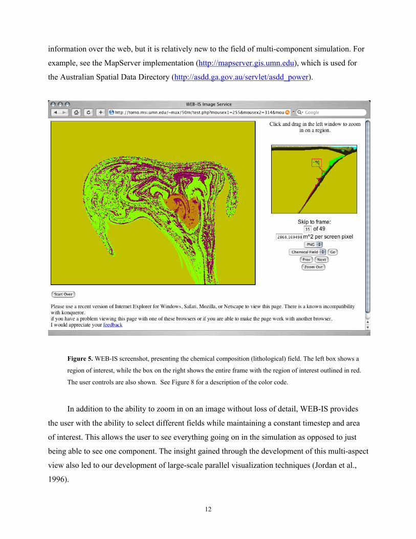
The WEB-IS image service (Fig. 5) incorporates a zoom feature in order to achieve high-
resolution visualization. The user is first presented with a scaled-down image of the data from our
simulation. An area of interest can be selected and our software then automatically creates a large
image of the selected region and displays it. An accompanying legend illustrates the relationship
of the enlarged region to the entire image. A recently developed feature allows the user to zoom
to a specific spatial resolution defined by the physical dimensions of the region of interest. This
feature allows geoscientists working remotely to maintain a better understanding of the scale of
the simulation thatn would otherwise be possible. The zoom functionality is made possible
through cooperation between JavaScript and PHP. When the user clicks and drags to select a
region of interest using JavaScript, the web browser transmits information about the region to the
server. Using PHP and the GD image library, a new image containing the region of interest is
created and sent to the user. This type of functionality has been influential in displaying map
12
information over the web, but it is relatively new to the field of multi-component simulation. For
example, see the MapServer implementation (http://mapserver.gis.umn.edu), which is used for
the Australian Spatial Data Directory (http://asdd.ga.gov.au/servlet/asdd_power).
Figure 5. WEB-IS screenshot, presenting the chemical composition (lithological) field. The left box shows a
region of interest, while the box on the right shows the entire frame with the region of interest outlined in red.
The user controls are also shown. See Figure 8 for a description of the color code.
In addition to the ability to zoom in on an image without loss of detail, WEB-IS provides
the user with the ability to select different fields while maintaining a constant timestep and area
of interest. This allows the user to see everything going on in the simulation as opposed to just
being able to see one component. The insight gained through the development of this multi-aspect
view also led to our development of large-scale parallel visualization techniques (Jordan et al.,
1996).

13
6) Visualization with large-screen display- Power Wall
Large data sets with many millions of pixels – the same as for high-resolution
photographs – can best be viewed on large display devices in order to obtain an entire panoramic
view. While the WEB-IS system is clearly our best option for remote visualization and small-
scale work on computer monitors, we saw the need for a large-scale alternative to WEB-IS.
Through our collaboration with the Laboratory for Computational Science and Engineering
(LCSE) at the University of Minnesota, we have gained access to a large display wall that is very
well suited for the parallel visualization of subduction zones (Fig 6).
Figure 6. Photograph of the LCSE PowerWall with movies playing on all ten panels. Total size of the
PowerWall is 7 feet high and 23 feet wide (2 x 6 meters).
We note that WEB-IS also enables display on other large-display devices, as one of the authors,
Dave Yuen, has done in July 2003 by transmitting the subduction dynamics via Internet from
Minnesota to a display wall at Florida State University, about 2200 kilometers away. In the
future, presentations involving large data sets will be conducted by using the next generation
Internet, whose transmission rate is around 10 Gbits/sec. This method of presentation makes more
sense with larger bandwidth in Web communication (Gilder, 2000). Our strategy for

14
visualization, as shown in Fig. 7, combines the remote visualization advantages of WEB-IS with
the large-scale, high-resolution advantages of devices like the PowerWall.
Figure 7. Overview of our visualization strategy, showing progression from raw data to visualization via
WEB-IS or the PowerWall.
Located in the Laboratory for Computational Science and Engineering (LCSE:
http://www.lcse.umn.edu), headed by Paul Woodward, the PowerWall is a high-performance,
high-resolution visualization system for large-scale numerical simulations. An array of ten LCD
projectors are arranged to project a seamless image onto a large screen. The 13 million pixels of
the PowerWall display, which is 7 feet tall and 23 feet wide (2 x 6 meters), allow us to view
simulations or other data in unprecedented detail, or to view multiple fields simultaneously, so
huge amounts of information can be absorbed by the mind at a single glance. Using the Linux
application ImageMagick and a set of custom shell scripts, we are able to convert the same set of
images used for WEB-IS into a movie file that can be played on the PowerWall using player
software developed by the LCSE team. The PowerWall gives us the flexibility to play up to ten
movies simultaneously so that we can examine in great detail the evolution of the subduction
zone in multiple components. In Figure 8, we show a movie with 50 frames that portrays the

15
temporal development of the chemical composition field for a simulation using 50 million
markers.
Figure 8. Movie with 50 frames demonstrating the evolution of the chemical composition (lithological) field
over time. One frame is shown here, and the full movie is available at
http://tomo.msi.umn.edu/~max/movie.html The simulation shown here uses 50 to 100 million markers to
represent chemical (lithological) field with resolution 50x50 to 30x30 m. The color code is: White = air (top
of the model), light blue = sea water (top of the model), grin-brown (both darker and lighter) = solid
sedimentary rocks (below sea water and in subduction zone); very dark blue = solid basaltic oceanic crust
(upper portion of the oceanic crust immediately below sediments), black = solid gabbroic oceanic crust (lower
portion of the oceanic crust), light green = serpentinized mantle (within both the slab and the overriding plate)
yellow = unhydrated mantle (both slab and wedge), brown = hydrated unserpentinized (i.e. beyond the
stability field of serpentine) mantle, very light green = partially molten hydrated mantle (within plumes); dark
magenta = partially molten gabbroic crust (mostly within plumes), light magenta/pink = partially molten
basaltic crust (mostly within plumes), very light pink = partially molten sediments (mostly within plumes).
The major advantage of the large-screen strategy is the possibility of very detailed dynamic
representation of several (up to 10, optimally 2 to 4) fields of physical parameters. The observer
can easily change the scale of observation by changing the physical distance from the screen.
This mode of visualization provides the optimal set-up for studying both the temporal and causal
relationships between large-scale and small-scale phenomena. This can also be exploited as a
very powerful and convincing pedagogical tool for students in the geosciences
(http://www.geowall.org).

16
7) Perspectives and Conclusions
The use of large numbers of markers allows high-resolution modeling with complex
geometry (e.g., Fig. 2). Combined with our recently developed visualization technology, this
modeling allows dynamic representation of a subduction zone with a spatial resolution of 10 to
100 meters, the scale at which geologists collect and extrapolate their data. We are, therefore,
confident that high resolution modeling is an accessible tool for geologists and that presented
numerical results can be tested with geological data on subduction-related geological complexes.
Rapid propagation of “hydrous cold plumes” may wield important control over the spatial
distribution of volcanic and seismic activities in regions of subduction (Tamura, 1994; Hall and
Kincaid, 2001; Gerya and Yuen, 2003a). Our results also appear to be realistic, when they are
compared with the seismic data revealing the complexity of seismicity distributions at subduction
zones, especially near the Japanese Trench (Zhao et al., 2002). Negative seismic velocity
anomalies found in the Japanese arc constitute a particular feature that might be reinterpreted in
light of our results. Rather than regarding them as thermal anomalies (Tamura et al., 2002), we
interpret these low-seismic-velocity anomalies (Zhao et al., 2002) near Japan as indicating some
traces of water (Jung and Karato, 2001). The generation and propagation of incipient magma
chambers above slabs depends strongly on the dynamics imposed by the subduction rate and the
thermal constraints posed by the age of the slab and the asthenospheric circulation above the slab
(Davies and Stevenson, 1992; Gerya and Yuen, 2003a; Stern, 2002).
Data-centered collaboration on the GRID (Berman et al., 2003) in the emerging new fields
of geoinformatics and cyberinfrastructures is expected to revolutionize the geosciences in the
next several years. About twenty years ago, Olson et al. (1984) employed 40,000 markers in the
studies of mixing dynamics in mantle convection. Today we have reached about 100 million
markers. We can then anticipate a decade from now, in 2013, it is not unreasonable to expect the

17
bar to be raised to around 10 billion markers! Such a high density of markers would demand
entirely new visualization tools and strategies, as well as new approaches to data storage and
transmission. Table 1 shows the dependence of the size of required memory versus number of
markers for configurations in two dimensions, as described in this paper, and three dimensions,
which could be used in the future. Clearly, the increasing number of tracers for this study alone
highlights the increasing problems as growing numerical simulations push the limits of available
methods of processing, storage, and visualization.
Number ofmarkers
Memory in 2-D Memory in 3-D
5 million 70 Megabytes 90 Megabytes
50 million 700 Megabytes 900 Megabytes
500 million 7 Gigabytes 9 Gigabytes
5 billion 70 Gigabytes 90 Gigabytes
50 billion 700 Gigabytes 900 Gigabytes
500 billion 7 Terabytes 9 Terabytes
Table 1. The minimal number of bytes for one marker is calculated using four bytes for each coordinate,
four bytes for the temperature, and two bytes for chemical component type. Therefore, one marker uses 14
bytes in two dimensions and 18 bytes in three dimensions. The memory required for various numbers of
markers is shown here.
Communications will improve drastically with the Next Generation Internet (Berman et
al., 2003). Many information technology experts predict that grids of geographically distributed
mass storage across the country along with strategically-located high-performance computers and
visualization platforms connected via high-speed (10 Gbit/sec to 50 Gbit/sec) networks will allow
geoscientists to collaborate seamlessly and remotely. A new era of integrated massive data from
distributed, diverse locations will aid earth scientists in discovering new phenomena by data-
mining and attacking problems across multiple spatio-temporal scales and at the same time
traverse over traditional discipline boundaries. The Earth Simulator Center
(http://www.es.jamstec.go.jp/esc/eng/) is an example of such an interdisciplinary endeavour, and
combines computer science with oceanic, atmospheric, and solid earth simulations. Large output

18
files from simulations at Earth Simulator contain a great deal of data, but are difficult to
postprocess or visualize in a rapid manner, underscoring the dire need for new visualization tools.
As shown in Table 1, 500 billion markers in three dimensions would require nearly 10 terabytes
of memory – around the same order of magnitude as the maximum capacity of Earth Simulator
and would produce total output on the order of 500 terabytes. These kinds of extreme problems in
computational geophysics motivate and shape new strategies in information technology in the
geosciences.
Data-centric collaboration of these problems will be undoubtedly carried out on the GRID
(Berman et al., 2003), which will revolutionize all of the geosciences in the next several years. In
this condition, WEB-IS will gain greater importance for remote visualization as the amount of
data in numerical experiments continues to grow. The problems created by large datasets are not
unique to the geosciences. Due to its data independence, WEB-IS can be used for remote data
query and visualization of biomedical problems, such as the analysis of archived mammograms
(http://nscp.upenn.edu/NDMA/), which have a deep social relevance since there is also a need for
ultra-large data systems, data-mining, and efficient access to a very large-scale dataset, in the
range of petabytes. WEB-IS also has potential applications in astronomy (Murtagh et al., 2002)
and in radar interferometry (Fialko and Simons, 2000), where there is a mounting need for
viewing data from multiple spectra and viewing high-resolution images involving billions of
pixels.
As large display devices like the LCSE PowerWall become cheaper – below the $5000
barrier – and also widespread and standardized, high-resolution parallel visualization will gain
greater acceptance as the method of choice for viewing multi-component numerical simulations.
In this regard, the GeoWall (http://www.geowall.org) can be a good role model for the
geosciences.
Because of interdisciplinary activities and feedback from information technology, we see a
very bright future lying ahead for visualization in the geosciences, both in large-scale numerical
simulations and high-resolution imaging from transmission electron microscopes (TEM), atomic

19
force microscopes (AFM), and magnetic resonance imaging (MRI). Technological breakthroughs
using liquid crystals and polymers will make electronic paper a viable medium, as well as more
portable PowerWalls. All of these developments together will help WEB-IS to fully fuel the rate
of progress in visualization in the geosciences.
Acknowledgements
We thank Yunsong Wang, Gordon Erlebacher, Zack Garbow, Ben Kadlec, Evan F. Bollig,
Erik O. D. Sevre, Paul Woodward, David H. Porter, and Michael Bakhos for discussions. This
research has been supported by the National Science Foundation. M. Rudolph thanks the
Research Experiences for Undergraduates program of the National Science Foundation, in
particular. T. Gerya appreciates support by the Russian Foundation of Basic Research grant no.
03-05-64633, by the Alexander von Humboldt Foundation Research Fellowship, and by the
German Science Foundation within SFB 526.
References
Berman F., Fox G., and Hey T. (2003) Grid Computing: Making the Global Infrastructure a
Reality. John Wiley and Sons.
Boggs J.B. and Yuen D.A. (2001) Wireless Internet access across Washington Avenue.
University of Minnesota Supercomputing Institute Research Report UMSI 2001/135,
November 2001. http://www.msi.umn.edu/~boggsj/wireless.html
Davies J.H. and Stevenson D.J. (1992) Physical model of source region of subduction zone
volcanics. Journal of Geophysical Research 97: 2037-2070.
Fialko Y. and Simons M. (2000) Deformation and seismicity in the Coso geothermal area, Inyo
County, California: observations and modeling using satellite radar interferometry.
Journal of Geophysical Research 105: 21781-21793.
Garbow Z.A., Erlebacher G., Yuen D.A., and Boggs, J.M. (2001) Interactive Web-based map:
applications to large data sets in the geosciences. Electronic Geosciences, 6.
Garbow Z.A., Yuen D.A., Erlebacher G., Bollig E.F., and Kadlec B.J. (2003) Remote
visualization and cluster analysis of 3-D geophysical data over the Internet using off-
screen rendering. Visual Geosciences (submitted).

20
Gilder G. (2000) Telecosm: How infinite bandwidth will revolutionize our world. New Press.
Gerya T.V. and Yuen D.A. (2003a) Rayleigh-Taylor instabilities from hydration and melting
propel ‘cold plumes’ at subduction zones. Earth and Planetary Science Letters 212:
47–62.
Gerya T.V. and Yuen D.A. (2003b) Characteristics-based marker method with conservative
finite-differences schemes for modeling geological flows with strongly variable transport
properties. Phys. Earth Planet. Inter. 140: 295-320.
Gerya T.V., Stoeckhert B., and Perchuk A.L. (2002) Exhumation of high-pressure metamorphic
rocks in a subduction channel - a numerical simulation. Tectonics 21: 6-1 - 6-19.
Gerya T.V., Yuen D.A., and Sevre E.O.D. (2004) Dynamical causes for incipient magma
chambers above slabs. Geology (in press).
Hall P.S. and Kincaid C. (2001) Diapiric flow at subduction zones: A recipe for rapid transport.
Science 292: 2472–2475.
Hockney R.W. and Eastwood J.W. (1981) Computer Simulations Using Particles. New York,
McGraw-Hill.
Jordan K.E., Yuen D.A., Reuteler D.M., Zhang S., and Haimes R. (1996) Parallel interactive
visualization of 3-D mantle convection. IEEE Computational Science and Engineering,
Vol. 3, No. 4: 29-37.
Jung, H., and Karato, S. (2001) Water-induced fabric transitions in olivine. Science, 293,
1460–1463.
Kincaid C. and Hall P.S. (2003) Role of back arc spreading in circulation and melting of
subduction zones. Journal of Geophysical Research 108, 7-1 – 7-14.
Marsh B.D. (1979) Island-arc development: some observation, experiments and speculations.
Journal of Geology 87: 687-713.
Murtagh F., Starck J.L and Louys M. (2002) Distributed visual information management in
astronomy. Computers in Science and Engineering Vol. 4 No. 6: 14-23.
Olson P.L., Yuen D.A., and Balsiger D.S. (1984) Mixing of passive heterogeneities by mantle
convection. J. Geophys. Res. 89: 425-436.
Osher S.J. and Fedkiw R. (2002) Level Set Methods and Dynamic Implicit Surfaces. NewYork,
Springer Verlag.
21
Peacock S.M. (2003) Thermal stucture and metamorphic evolution of subducting slabs. In: Eiler
J.M. and Abers G. (eds) The Subduction Factory. AGU Gophysical Monograph,
American Geophysical Union, Washington, D. C. (in press).
Ranalli G. (1995) Rheology of the Earth (2nd edition). London, Chapman and Hall.
Sapiro G. (2001) Geometric Partial Differential Equations. Cambridge University Press.
Schmidt M.W. and Poli S. (1998) Experimentally based water budgets for dehydrating slabs and
consequences for arc magma generation. Earth Planet. Sci. Lett. 163: 361-379.
Stern R.J. (2002) Subduction zones. Review in Geophysics 40: 3-1 – 3-38.
Tamura, Y. (1994) Genesis of island arc magmas by mantle-derived bimodal magmatism:
Evidence from the Shirahama Group, Japan. Journal of Petrology, 35: 619–645.
Tamura Y., Tatsumi Y., Zhao D.P., Kido Y., and Shukuno H. (2002) Hot fingers in the mantle
wedge: new insights into magma genesis in subduction zones. Earth and Planetary
Science Letters 197: 105–116.
Ten A.A., Yuen D.A., and Podladchikov Yu.Yu. (1999) Visualization and analysis of mixing
dynamical properties in convecting systems with different rheologies. Electronic
Geosciences 4.
Tovish A., Schuberst G., and Luyendyk B.P. (1978) Mantle flow pressure and the angle of
subduction: non-Newtonian cornerflows. J. Geophys. Res. 83: 5892-5898.
Wang Y., Bollig E.F., Kadlec B.J., Garbow Z.A., Erlebacher G., Yuen D.A., Rudolph M., Sevre,
E.O.D, and Yang L. (2003) WEB-IS (Integrated System): an overall view. Visual
Geosciences (in preparation).
Yang X., Wang Y., Bollig E.F., Kadlec B.J., Garbow Z.A., Yuen D.A., and Erlebacher G. (2003)
WEB-IS2: Next generation web services using Amira visualization package. AGU Fall
Meeting, Abstract NG11A-0164.
Zhao, D.P., Mishra, O.P., and Sandra, R. (2002) Influence of fluid and magma on earthquakes:
Seismological evidence. Physics of the Earth and Planetary Interiors, 132, 249–267.