maximum non-extensive entropy block bootstrap · 2015-03-02 · buhlmann (1997) develops a...

Overview&Motivation MEB MEBB Simulation of the MEBB MnEBB Conclusions References

Maximum Non-extensive Entropy BlockBootstrap

Jan NovotnyCEA, Cass Business School & CERGE-EI

(with Michele Bergamelli & Giovanni Urga)

4-5 September 201415th OxMetrics User Conference

Cass Business School

J. Novotny (Cass Business School, UK) 4-5 September 2014 – 15th OxMetrics User Conference – London 1/27

mailto:[email protected]


Overview

• In this paper, we propose a correct maximum entropy-based resampling scheme— the Maximum Entropy Block Bootstrap (MEBB) — valid for non-stationarydata.

• We illustrate the performance of our procedure on the unit root test —Dickey-Fuller test.

• We extend the MEBB by considering the generalized notion of entropy andintroduce the Maximum non-extensive Entropy Block Bootstrap which allows forfat tails.

• We provide a Monte Carlo simulation to show the properties of the MnEBB.




Literature Review I

• Since Efron (1979) for identically and independent distributed (iid) data, thebootstrap method has been extended to handle more complex data structures.

• Time-series data may fail to satisfy the iid-ness

1. The data distribution might change over time

2. The observations are mutually dependent – memory in the process

We focus on the case 2: Mutually dependent observations:

• Kunsch (1989) proposes the non-parametric block bootstrap technique whichinvolves re-sampling blocks of data rather than individual observations.

• Buhlmann (1997) develops a parametric alternative usually called sieve bootstrapwhich circumvents the dependence structure in the data by first fitting an AR(p)process – where p grows with the sample size T – and then resampling fromsupposedly iid residuals.

• For other resampling schemes, see Politis, Romano, and Wolf (1999) for anoverview.

It works well for the time series when the dependence dies out over time......yet, in economics and finance, we frequently study relationships that involveintegrated processes, mostly I (1).




Literature Review II

• The problem of interest is in bootstrapping test procedures to assess the unitroot hypothesis.

• Two approaches to chose from:

1. Resample the first differences and treat the dependence in differences, see, e.g.,Palm, Smeekes, and Urbain (2007) for a review

2. Resample directly from the original non-differenced data

• With respect to the case 2:

• The major benefit: we can ignore the dependence structure in the firstdifferences; though still uncommon

• The only valid (in the sense of consistency of the bootstrap procedure)method proposed in the statistical literature is the Continuous Path BlockBootstrap of Paparoditis and Politis (2001)

• Theoretical validation of the block bootstrap consistency is provided byPhillips (2010), who uses a different algorithm to Paparoditis and Politis(2001) – Phillips method is inconsistent under the alternative

• Alternative proposed by Vinod and Lopez-de Lacalle (2009) – MaximumEntropy Bootstrap – based on maximum entropy principle and perfect rankcorrelation – significant flaws.

→ Maximum (Non-)extensive Entropy Block BootstrapJ. Novotny (Cass Business School, UK) 4-5 September 2014 – 15th OxMetrics User Conference – London 4/27



Maximum Entropy Bootstrap (MEB)

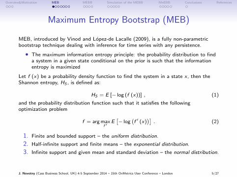
MEB, introduced by Vinod and Lopez-de Lacalle (2009), is a fully non-parametricbootstrap technique dealing with inference for time series with any persistence.

• The maximum information entropy principle: the probability distribution to finda system in a given state conditional on the prior is such that the informationentropy is maximized

Let f (x) be a probability density function to find the system in a state x , then theShannon entropy, HS , is defined as:

HS = E [− log (f (x))] , (1)

and the probability distribution function such that it satisfies the followingoptimization problem

f = arg maxf ′

E[− log

(f ′ (x)

)]. (2)

1. Finite and bounded support – the uniform distribution.

2. Half-infinite support and finite means – the exponential distribution.

3. Infinite support and given mean and standard deviation – the normal distribution.




The MEB Algorithm

Let us consider X = x1, . . . , xT → order statistics as x(t). Support of the order

statistics x(t) ∈[x(0), x(T+1)

]. We define the midpoints zt as

z0 = x(0) , zt =1

2

(x(t) + x(t+1)

), t ∈ {1, . . . ,T − 1} , zT = x(T+1) .

Using the midpoints, we define T half-open intervals It = (zt−1, zt ] around eachobservation.The maximum entropy density function is solution to (2) with:a. The mass preserving constraint imposed on the density function states that, onaverage, 1/T of the mass of the density function lies in each of the intervals It .b. The mean preserving constraint states that

T∑t=1

xt =T∑t=1

x(t) =T∑t=1

mt ,

where mt is the mean of f over the interval It .

MEB = Max. Entropy+Mass Preserving+Mean Preserving+Perfect Rank Correlation




The MEB Algorithm – cont’dTo create a single realization xt → x∗t , the MEB is based on the following algorithm:

1. Order statistics x(t) based on xt and define the support of the order statistics[x(0), x(T+1)

]with x(0) = x(1) − dtrm and x(T+1) = x(T ) + dtrm, with

dtrm = Etrim

[∣∣x(t) − x(t−1)

∣∣].2. We define a T × 2 sorting matrix, S1, and place the index set t = {1, . . . ,T} in

the first column and the observed time series xt in the second column.

3. We sort the matrix S1 with respect to the second column, xt , and define theorder statistics x(t). We then define the midpoints zt and the half-open intervalsIt .

4. We draw T uniform pseudo-random numbers ps ∼ U [0, 1], with s ∈ {1, . . . ,T}and assign the range Rt =

(tT, t+1

T

]for t ∈ {0,T − 1} wherein each ps falls.

5. We match each Rt with It and using the density function defined above, we drawthe new set x∗t .

6. We define a corresponding T × 2 sorting matrix S2, analogous to S1. We sortthe T elements x∗t in an increasing order of the magnitude to form the orderingstatistics x∗

(t).

7. We replace the second column of S1, the order statistics x(t), by the secondcolumn of S2, the order statistics x∗

(t)of the newly generated set. We sort the

x∗(t)

based on the first column of S1, and thus recover x∗t . The set x∗t represents

a resampled set of observations xt .J. Novotny (Cass Business School, UK) 4-5 September 2014 – 15th OxMetrics User Conference – London 7/27



The Maximum Entropy Bootstrap to Assess the Unit RootHypothesis

Let us consider a standard AR(1) process frequently used in the econometric analysis

yt = ρ · yt−1 + εt , (3)

where εt ∼ i.i.d.N (0, 1). In this paper we focus on the unit root case, i.e., ρ = 1. Weconsider 100 points and y0 = 0.

xt x*t

0 10 20 30 40 50 60 70 80 90 100

-10.0

-7.5

-5.0

-2.5

0.0

2.5

5.0xt x*

t




Size of the Test to Reject the Null

We employ the MEB to assess the rejection frequency of the test with null hypothesisρ = 1 against the alternative of ρ < 1: The empirical rejection frequencies to assessthe quantile of the bootstrap distribution of the t-statistic.

45 Line MEB

0.0 0.1 0.2 0.3 0.4 0.5 0.6 0.7 0.8 0.9 1.0

0.1

0.2

0.3

0.4

0.5

0.6

0.7

0.8

0.9

1.0 45 Line MEB

We perform a 1000 replications of the true data generating process and for eachreplication, we create 299 bootstrap samples. We consider T = 100 and initial pointto be set at y0 = 0.




Why the Maximum Entropy Bootstrap Fails?• Reason to Fail 1: The distribution of the MEB statistic is on average more

dispersed than that of the statistic itself.

• Assessment 1: The figure reports the distribution of the original t-statistic andone corresponding bootstrapped replication under H0 : ρ = 1, using 1000replications under the null.

τ τ*

-4 -3 -2 -1 0 1 2 3 4

0.05

0.10

0.15

0.20

0.25

0.30

0.35

0.40τ τ*




Why the Maximum Entropy Bootstrap Fails?

• Reason to Fail 2: For each replication, the bootstrap statistics are positivelycorrelated with the true statistic and the bootstrap does not provide anindependent draw of a sample.

• Assessment 2: We estimate the correlation between the t-statistics of the datagenerating process, τi , and the t-statistics of the MEB, τ∗i , using the OLS:

τ∗i = − 0.2452(0.00326)

+ 0.8728(0.00299)

τi i = 1, . . . , 1000 .(4)

The adjusted R2 = 0.9445 suggests that the t-statistic of the MEB is too close to thedata generating process.

• The strong positive correlation between the two t-statistics suggests that theMEB is not a consistent method. Further, the failure is in the lack of variation inthe MEB sample. The MEB in fact mimics the data generating process tooclosely

MEB = Max. Entropy+Mass Preserving+Mean Preserving+PerfectRankCorrelation




Maximum Entropy Block Bootstrap

We introduce the Maximum Entropy Block Bootstrap (MEBB), which preserves theperfect rank correlation locally and is free of tail trimmings.The MEBB AlgorithmStep AWe choose the block length ` < T and let i0, i1, . . . , ik−1 i.i.d. uniform randomnumbers on the set [1, 2, . . . ,T − `] where k = bT/`c, (number of blocks).Step BFor each ij , with j = 0, . . . , k − 1, we get the subset of the original time series

X (j) ={xij , xij+1, . . . , xij+`−1

}and apply the Paparoditis and Politis (2001)

demeaning.Step CWe apply the MEB algorithm corresponding to Steps 1-7 in Section 2 for each subset

X (j) separately and generate X∗(j) ={x∗ij, x∗ij+1, . . . , x

∗ij+`−1

}.

Step DWe recover the bootstrapped sample path by sewing the X∗(1), . . . ,X∗(k) such thatx∗ij+1

− x∗ij+`−1 is set in a way to correspond to the difference xij+1− xij+`−1.

Step EIf the length of the bootstrapped sample path is exceeding T , we take the first Tvalues.




cont’d

• We omit the trimming: Step 1 in the MEB algorithm is modified as follows:

Step 1*We create an order statistics x(t) based on the empirical data set xt and define thesupport of the empirical data to be [−∞,∞]. The constrained solution for themaximum entropy distribution on the half-open interval [0,∞) is given by f = λe−λx

with mass at 1/λ. Therefore, for the intervals I1 ≡ (−∞, z1] and IT ≡ [zT ,∞),respectively, is given by

fI1 (x) = β1λ1e−λ1(z1−x) , x ∈ I1 , m1 =

3x(1)

4+

x(2)

4(5)

fIT (x) = βTλT e−λT (x−zT ) , x ∈ IT , mT =

x(T−1)

4+

3x(T )

4, (6)

where the parameters λ1 and λT are set such that the mean preserving constraintsimposed on m1 and mT are satisfied.

• Finally, Steps 2-7 of the MEBB algorithm for a given subset X∗ are the same asfor the MEB.

Such a modified algorithm — MEBB — preserves the perfect rank correlation locallyand uses the proper form of the tails in the maximum entropy distribution function.




A Numerical Illustration

We report a bootstrap sample path based on the new MEBB algorithm.

xt x*t

0 10 20 30 40 50 60 70 80 90 100

-10.0

-7.5

-5.0

-2.5

0.0

2.5

5.0xt x*

t

The sample path xt and the replicated path x∗t by the MEBB. The true datagenerating process is given as yt = yt−1 + εt , with εt ∼ N (0, 1), y0 = 0, and T = 100.




Does the Correction Work?

Reason to Fail 1: The right panel depicts the distribution of the original t-statisticand one corresponding bootstrapped replication under H0 : ρ = 1.

τ τ*

-4 -3 -2 -1 0 1 2 3 4

0.05

0.10

0.15

0.20

0.25

0.30

0.35

0.40 τ τ*

Reason to Fail 2: Indeed, a regression similar to the one above gives

τ∗i = − 0.4541(0.0354)

− 0.005663(0.0323)

τi i = 1, . . . , 1000, (7)

with the adjusted R2 = 0.00097.

No problem detected!




Monte Carlo Simulation Study

Focus: bootstrapping the t-statistic distribution for the AR(1) coefficient.Benchmark: the standard residuals-based bootstrap (RB) and continuous path blockbootstrap(CPBB)The data generating process:

ym,t = ρ0ym,t−1 + ηm,t

ym,0 = 0 t = 1, . . . ,T ,

with m denoting a realizations of the sample path, and where we let ρ0 = 1 fordifferent sample lengths T = {50, 100, 300} in order to assess the size andρ0 = {0.99, 0.95, 0.90, 0.80, 0.70, 0.60, 0.5} to assess power. Moreover, we generatethe {ηm,t} series allowing for “progressive” fat-tails: N (0, 1), T (5), T (3).Test statistic: We fit an AR(1) model and compute the t-statistic

tm =ρm − 1

σηm (∑T

t=1 y2m,t−1)−1/2

, for testing

{H0 : ρ = 1H1 : |ρ| < 1

(8)

where ρm =(∑T

t=1 y2m,t−1

)−1 (∑Tt=1 ym,t−1ym,t

)is the least squares estimator of

the autoregressive coefficient and σηm = (T − 1)−1/2(∑T

t=1 η2m,t)

1/2 is the residualsstandard deviation.




Benchmark Bootstrap MethodsResiduals Bootstrap

y∗b,m,0 = ym,0

y∗b,m,t = ρ0y∗b,m,t−1 + η∗b,m,t t = 1, . . . ,T

where η∗b,m,t are drawn from the centered residuals{ηm,t − 1

T

∑Tt=1 ηm,t

}T

t=1obtained from the residuals of the regression of yb,m,t on its first lag.Continuous Path Block BootstrapFollowing Paparoditis and Politis (2001):

1. Compute the centered residuals

um,t = ym,t−ym,t−1−1

T − 1

T∑t=1

(ym,t−ym,t−1) with ym,t =

{ym,1 t = 1ym,1 +

∑tj=2 um,j t = 2, . . . ,T .

2. Choose the block length ` < T and let i0, i1, . . . , ik−1 i.i.d. uniform randomnumbers on the set [1, 2, . . . ,T − `], where k = bT/`c (number of blocks).

3. Build the bootstrapped series of length l = k · ` as

y∗b,m,jy∗b,m,rs+j = ym,1 + [yi0+j−1 − yi0 ] first block , = y∗b,m,r` + [yim+j − yir ] (r + 1)th block

for j = 1, . . . , ` and r = 1, . . . , k − 1.J. Novotny (Cass Business School, UK) 4-5 September 2014 – 15th OxMetrics User Conference – London 17/27



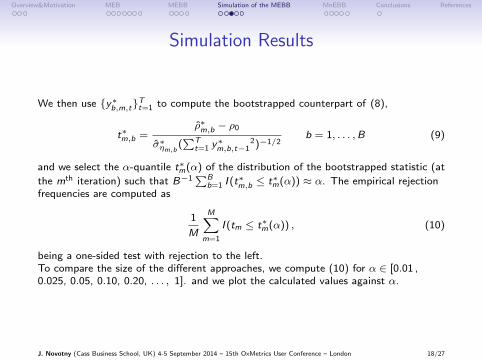
Simulation Results

We then use {y∗b,m,t}Tt=1 to compute the bootstrapped counterpart of (8),

t∗m,b =ρ∗m,b − ρ0

σ∗ηm,b (∑T

t=1 y∗m,b,t−1

2)−1/2b = 1, . . . ,B (9)

and we select the α-quantile t∗m(α) of the distribution of the bootstrapped statistic (at

the mth iteration) such that B−1∑B

b=1 I (t∗m,b ≤ t∗m(α)) ≈ α. The empirical rejection

frequencies are computed as

1

M

M∑m=1

I (tm ≤ t∗m(α)) , (10)

being a one-sided test with rejection to the left.To compare the size of the different approaches, we compute (10) for α ∈ [0.01 ,0.025, 0.05, 0.10, 0.20, . . . , 1]. and we plot the calculated values against α.




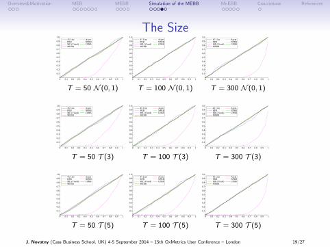
The Size45 Line PRB ME (Vinod) MEBB

Asym NPRB CPBB

0 0.1 0.2 0.3 0.4 0.5 0.6 0.7 0.8 0.9 1

0.1

0.2

0.3

0.4

0.5

0.6

0.7

0.8

0.9

1.045 Line PRB ME (Vinod) MEBB

Asym NPRB CPBB

T = 50 N (0, 1)

45 Line PRB ME (Vinod) MEBB

Asym NPRB CPBB

0 0.1 0.2 0.3 0.4 0.5 0.6 0.7 0.8 0.9 1

0.1

0.2

0.3

0.4

0.5

0.6

0.7

0.8

0.9


Asym NPRB CPBB

T = 100 N (0, 1)


Asym NPRB CPBB

0 0.1 0.2 0.3 0.4 0.5 0.6 0.7 0.8 0.9 1

0.1

0.2

0.3

0.4

0.5

0.6

0.7

0.8

0.9


Asym NPRB CPBB

T = 300 N (0, 1)


Asym NPRB CPBB

0 0.1 0.2 0.3 0.4 0.5 0.6 0.7 0.8 0.9 1

0.1

0.2

0.3

0.4

0.5

0.6

0.7

0.8

0.9


Asym NPRB CPBB

T = 50 T (3)


Asym NPRB CPBB

0 0.1 0.2 0.3 0.4 0.5 0.6 0.7 0.8 0.9 1

0.1

0.2

0.3

0.4

0.5

0.6

0.7

0.8

0.9


Asym NPRB CPBB

T = 100 T (3)

45 Line RPB ME (Vinod) MEBB

Asym NPRB CPBB

0 0.1 0.2 0.3 0.4 0.5 0.6 0.7 0.8 0.9 1

0.1

0.2

0.3

0.4

0.5

0.6

0.7

0.8

0.9

1.045 Line RPB ME (Vinod) MEBB

Asym NPRB CPBB

T = 300 T (3)


Asym NPRB CPBB

0 0.1 0.2 0.3 0.4 0.5 0.6 0.7 0.8 0.9 1

0.1

0.2

0.3

0.4

0.5

0.6

0.7

0.8

0.9


Asym NPRB CPBB

T = 50 T (5)


Asym NPRB CPBB

0 0.1 0.2 0.3 0.4 0.5 0.6 0.7 0.8 0.9 1

0.1

0.2

0.3

0.4

0.5

0.6

0.7

0.8

0.9


Asym NPRB CPBB

T = 100 T (5)


Asym NPRB CPBB

0 0.1 0.2 0.3 0.4 0.5 0.6 0.7 0.8 0.9 1

0.1

0.2

0.3

0.4

0.5

0.6

0.7

0.8

0.9


Asym NPRB CPBB

T = 300 T (5)




The Power

Asym NPRB CPBB

PRB ME (Vinod) MEBB

0.5 0.55 0.6 0.65 0.7 0.75 0.8 0.85 0.9 0.95

0.1

0.2

0.3

0.4

0.5

0.6

0.7

0.8

0.9

1.0

Asym NPRB CPBB

PRB ME (Vinod) MEBB

T = 50 N (0, 1)

Asym NPRB CPBB

PRB ME (Vinod) MEBB

0.5 0.55 0.6 0.65 0.7 0.75 0.8 0.85 0.9 0.95

0.1

0.2

0.3

0.4

0.5

0.6

0.7

0.8

0.9

1.0

Asym NPRB CPBB

PRB ME (Vinod) MEBB

T = 100 N (0, 1)

Asym NPRB CPBB

PRB ME (Vinod) MEBB

0.5 0.55 0.6 0.65 0.7 0.75 0.8 0.85 0.9 0.95

0.1

0.2

0.3

0.4

0.5

0.6

0.7

0.8

0.9

1.0

Asym NPRB CPBB

PRB ME (Vinod) MEBB

T = 300 N (0, 1)

Asym NPRB CPBB

PRB ME (Vinod) MEBB

0.5 0.55 0.6 0.65 0.7 0.75 0.8 0.85 0.9 0.95

0.1

0.2

0.3

0.4

0.5

0.6

0.7

0.8

0.9

1.0

Asym NPRB CPBB

PRB ME (Vinod) MEBB

T = 50 T (3)

Asym NPRB CPBB

PRB ME (Vinod) MEBB

0.5 0.55 0.6 0.65 0.7 0.75 0.8 0.85 0.9 0.95

0.1

0.2

0.3

0.4

0.5

0.6

0.7

0.8

0.9

1.0

Asym NPRB CPBB

PRB ME (Vinod) MEBB

T = 100 T (3)

Asym NPRB CPBB

PRB ME (Vinod) MEBB

0.5 0.55 0.6 0.65 0.7 0.75 0.8 0.85 0.9 0.95

0.1

0.2

0.3

0.4

0.5

0.6

0.7

0.8

0.9

1.0

Asym NPRB CPBB

PRB ME (Vinod) MEBB

T = 300 T (3)

Asym NPRB CPBB

PRB ME (Vinod) MEBB

0.5 0.55 0.6 0.65 0.7 0.75 0.8 0.85 0.9 0.95

0.1

0.2

0.3

0.4

0.5

0.6

0.7

0.8

0.9

1.0

Asym NPRB CPBB

PRB ME (Vinod) MEBB

T = 50 T (5)

Asym NPRB CPBB

PRB ME (Vinod) MEBB

0.5 0.55 0.6 0.65 0.7 0.75 0.8 0.85 0.9 0.95

0.1

0.2

0.3

0.4

0.5

0.6

0.7

0.8

0.9

1.0

Asym NPRB CPBB

PRB ME (Vinod) MEBB

T = 100 T (5)

Asym NPRB CPBB

PRB ME (Vinod) MEBB

0.5 0.55 0.6 0.65 0.7 0.75 0.8 0.85 0.9 0.95

0.1

0.2

0.3

0.4

0.5

0.6

0.7

0.8

0.9

1.0

Asym NPRB CPBB

PRB ME (Vinod) MEBB

T = 300 T (5)




The Maximum non-extensive Entropy Block BootstrapThe key concept of our framework is the generalized Tsallis (1988) entropy:

Hq = −1

1− q

(1−

N∑i=1

(pi )q

)→ Hq = −

1

1− q

(1−

∫dx (p (x))q

),

where the parameter q governs the non-extensiveness of the system. The Tsallisentropy converges to the Shannon entropy in the limit when q → 1.For a given q, the density function fq is given as

fq (x) =[1− β (1− q) x]1/(1−q)

Zq, Zq =

∫dx [1− β (1− q) x]1/(1−q)

. (11)

Some Properties:

• The non-extensiveness: Hq (A + B) = Hq (A) + Hq (B) + (1− q)Hq (A)Hq (B).

• The limit of this distribution function is exponential function for q → 1.

• For q ∈ (1, 2): power law behavior & fat tails.

• For q < 1: non-standard behavior – f is infinite over the semi-definite intervaland thus it requires a normalization by an infinite normalization factor.

• As q → 0, we get uniform distribution, or, fq→0 (x) = c/∞, where c does notdepend on x . For q > 5/3, we get a distribution with non-existing secondmoment, or E

[x2]

=∞.

• At q = 2, the first moment cease to exist.

• We consider q ∈ [1, 5/3).J. Novotny (Cass Business School, UK) 4-5 September 2014 – 15th OxMetrics User Conference – London 21/27



The MnEBB Algorithm

Considering non-extensive entropy:

fq (x) = αq (1 − β (1 − q) x)1

1−q , x ∈ I1 m1 =3x(1)

4+

x(2)

4(12)

αq :

∫I1

xdxfq (x) = m1 (13)

fq (x) =1

zk − zk−1

, x ∈ Ik∣∣k=2,...,T−1 mk =

x(k−1)

4+

x(k)

2+

x(k+1)

4(14)

fq (x) = ωq (1 − β (1 − q) x)1

1−q , x ∈ IT mT =x(T−1)

4+

3x(T )

4(15)

ωq :

∫IT

xdxfq (x) = mT (16)

• The remaining structure of the MnEBB algorithm is just as defined for theMEBB.

• The choice of q > 1 suggests using the distribution with fatter tails than impliedby the standard entropy.




Illustration of the MnEBB

The figure reports the sample path xt and the replicated path x∗t by the MnEBB withq = 1.25 and q = 1.5.

xt x*t with q=1.5 x*

t with q=1.25

0 10 20 30 40 50 60 70 80 90 100

-10.0

-7.5

-5.0

-2.5

0.0

2.5

5.0 xt x*t with q=1.5 x*

t with q=1.25




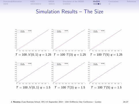
Simulation Results – The Size

45 Line MNEBB

MEBB

0 0.1 0.2 0.3 0.4 0.5 0.6 0.7 0.8 0.9 1

0.1

0.2

0.3

0.4

0.5

0.6

0.7

0.8

0.9

1.045 Line MNEBB

MEBB

T = 100 N (0, 1) q = 1.25

45 Line MNEBB

MEBB

0 0.1 0.2 0.3 0.4 0.5 0.6 0.7 0.8 0.9 1

0.1

0.2

0.3

0.4

0.5

0.6

0.7

0.8

0.9

1.045 Line MNEBB

MEBB

T = 100 T (3) q = 1.25

45 Line MNEBB

MEBB

0 0.1 0.2 0.3 0.4 0.5 0.6 0.7 0.8 0.9 1

0.1

0.2

0.3

0.4

0.5

0.6

0.7

0.8

0.9

1.045 Line MNEBB

MEBB

T = 100 T (5) q = 1.25

45 Line MNEBB

MEBB

0 0.1 0.2 0.3 0.4 0.5 0.6 0.7 0.8 0.9 1

0.1

0.2

0.3

0.4

0.5

0.6

0.7

0.8

0.9

1.045 Line MNEBB

MEBB

T = 100 N (0, 1) q = 1.5

45 Line MNEBB

MEBB

0 0.1 0.2 0.3 0.4 0.5 0.6 0.7 0.8 0.9 1

0.1

0.2

0.3

0.4

0.5

0.6

0.7

0.8

0.9

1.045 Line MNEBB

MEBB

T = 100 T (3) q = 1.5

45 Line MNEBB

MEBB

0 0.1 0.2 0.3 0.4 0.5 0.6 0.7 0.8 0.9 1

0.1

0.2

0.3

0.4

0.5

0.6

0.7

0.8

0.9

1.045 Line MNEBB

MEBB

T = 100 T (5) q = 1.5




Simulation Results – The Power

MEBB MNEB

0.5 0.55 0.6 0.65 0.7 0.75 0.8 0.85 0.9 0.95

0.1

0.2

0.3

0.4

0.5

0.6

0.7

0.8

0.9

1.0

MEBB MNEB

T = 100 N (0, 1) q = 1.25

MEBB MNEB

0.5 0.55 0.6 0.65 0.7 0.75 0.8 0.85 0.9 0.95

0.1

0.2

0.3

0.4

0.5

0.6

0.7

0.8

0.9

1.0

MEBB MNEB

T = 100 T (3) q = 1.25

MEBB MNEB

0.5 0.55 0.6 0.65 0.7 0.75 0.8 0.85 0.9 0.95

0.1

0.2

0.3

0.4

0.5

0.6

0.7

0.8

0.9

1.0

MEBB MNEB

T = 100 T (5) q = 1.25

MEBB MNEBB

0.5 0.55 0.6 0.65 0.7 0.75 0.8 0.85 0.9 0.95

0.1

0.2

0.3

0.4

0.5

0.6

0.7

0.8

0.9

1.0

MEBB MNEBB

T = 100 N (0, 1) q = 1.5

MEBB MNEBB

0.5 0.55 0.6 0.65 0.7 0.75 0.8 0.85 0.9 0.95

0.1

0.2

0.3

0.4

0.5

0.6

0.7

0.8

0.9

1.0

MEBB MNEBB

T = 100 T (3) q = 1.5

MEBB MNEBB

0.5 0.55 0.6 0.65 0.7 0.75 0.8 0.85 0.9 0.95

0.1

0.2

0.3

0.4

0.5

0.6

0.7

0.8

0.9

1.0

MEBB MNEBB

T = 100 T (5) q = 1.5




Conclusion and Future Work

• We proposed the Maximum Entropy Block Bootstrap, a fully non-parametricbootstrap procedure, to sample directly the time series with a general persistencestructure.

• Our procedure: the maximum entropy principle and preserving locally the rankcorrelation between the true data generating process and the bootstrap draws.

• The unit root test suggests that our procedure performs well.

• We generalized the MEBB to the non-extensive entropy and introduce theMaximum non-extensive Entropy Bootstrap, which allows for inclusion of fattails and power-law behavior.

• This generalized procedure outperforms the Maximum Entropy Bootstrap forlarge values of the non-extensiveness even when the underlying data generatingprocess is the normal distribution.

• Future developments.

• To derive the limiting theory of the MEBB and MnEBB methods proposedin this paper.

• To extend the proposed procedure to alternative non-stationary frameworkssuch as co-integration analysis.

• To connect the non-extensiveness with the Hurt exponent.




References

Buhlmann, P. (1997). Sieve Bootstrap for Time Series. Bernoulli 3, 123–148.

Efron, B. (1979). Bootstrap Methods: Another Look at the Jackknife. Annals of Statistics 7, 1–26.

Kunsch, H. (1989). The Jack-knife and the Bootstrap for General Stationary Observations. Annalsof Statistics 17, 1217–1241.

Palm, F. C., S. Smeekes, and J.-P. Urbain (2007). Bootstrap Unit-Root Tests: Comparisons andExtensions. Journal of Time Series Analysis 29, 371–401.

Paparoditis, E. and D. Politis (2001). The Continuous Path Block-Bootstrap. In M. Puri (Ed.),Asymptotics in Statistics and Probability, pp. 305–320. VSP Publications.

Phillips, P. C. B. (2010). Bootstrapping I (1) Data. Journal of Econometrics 158, 280–284.

Politis, D., J. Romano, and M. Wolf (1999). Subsampling. Springer Series in Statistics. SpringerNew York.

Tsallis, C. (1988). Possible Generalization of Boltzmann-Gibbs Statistics. Journal of StatisticalPhysics 52(1-2), 479–487.

Vinod, H. D. and J. Lopez-de Lacalle (2009). Maximum Entropy Bootstrap for Time Series: themeboot R Package. Journal of Statistical Software 29, 1–19.



maximum non-extensive entropy block bootstrap · 2015-03-02 · buhlmann (1997) develops a...

Documents