maximum-likelihood soft-decision decoding of block … · tda progress report 42-117 n94-35555 p...
TRANSCRIPT

TDA Progress Report 42-117
N94-35555P
May 15, 1994
2
i
Maximum-Likelihood Soft-Decision Decoding
of Block Codes Using the
A* AlgorithmL. Ekroot and S. Dolinar
Communications Systems Research Section
The A* algorithm finds the path in a finite depth binary tree that optimizes a
function. Here, it is applied to maximum-likelihood soft-decision decoding of block
codes where the function optimized over the codewords is the likelihood function
of the received sequence given each codeword. Tile algorithm considers codewords
one bit at a time, making use of the most reliable received symbols first and pur-
suing only the partially" expanded codewords that might be maximally likely. A
version of the A* algorithm for maximum-likelihood decoding of block codes has
been implemented for block codes up to 64 bits in length. The efficiency of this
algorithm makes simulations of codes up to length 6,1 feasible. This article details
the implementation currently in use, compares the decoding complexity with that
of exhaustive search and Viterbi decoding algorithms, and presents performance
curves obtained with this implementation of the A* algorithm for several codes.
I. Introduction
The A* algorithm is an artificial intelligence algorithm
for finding the path in a graph that optimizes a fimction.
Nilsson [1, pp. 72-88] describes the algorithm as a heuris-
tic graph-search procedure and shows that the algorithm
terminates in an optimal path. The A* algorithm has been
used to implement full maximum-likelihood soft. decoding
of linear block codes by Han et al. [2-4].
The A* algorithm explores the codewords one bit at.
a time using the most reliable information first, pursuing
the most likely codewords first, and ruling out subopti-
mal codewords as soon as possible. The details of the A*
algorithm are covered in Section II. The implementation
discussed here has most of the features recommended in
[2] and has allowed code performance simulations for codes
up to length 64 ill reasonable amounts of time.
The codes considered here are binary linear codes. An
(N,K) code has 2 K codewords each of length N bits.
The binary symbols are transmitted over a communica-
tions channel and corrupted by channel noise. An additive
noise channel is one in which each received symbol can be
described as the sum of the signal and noise. The deep
space channel is accurately described as an additive white
Gaussian noise channel, meaning that the additive noise
for each symbol is an independent, random variable dis-
tributed according to a zero-mean Gaussian with variance
129
https://ntrs.nasa.gov/search.jsp?R=19940031048 2018-06-04T20:09:52+00:00Z

_r2. Therefore, the received symbols, ri for i = 1 .... , N,
that form the received sequence r are continuously valued
and are called soft symbols.
Binary antipodal signaling transmits the bits as signals
of equal magnitude, but different signs. For this article,
the ith bit, bi E {0, 1}, of the binary codeword b is trans-mitted as ci = (-t) b'. That is, a 0 is transmitted as +1,
and a 1 is transmitted as -1. Thus, the energy in a trans-N _ N" bi 2
nfitted codeword e is given by _i=1 c_" = }-'_,i:t((-1) ) =
N independently of the codeword sent. The signal-to-noise
ratio (SNR) is Eb/,'Vo, where Eb = N/K is the energy" per
information bit, and N0/2 = a 2 is the white Gaussian
noise two-sided spectral density. Thus, the SNR is given
by
N )(dB)SNR = 10logi0
The hard-limited symbol hi is the transmitted signalvalue +1 nearest to the received symbol ri; it is given by
ri
hi =sgn ri ) =
where hi equals 1 in the zero-probability case of ri = 0. If
the received symbols are individually hard-limited before
decoding, some information is lost from each symbol. For
instance, soft symbols like 0.01 and 1.01 both hard limit to
+1, yet the received value 1.01 is much more likely to havebeen transmitted as +1 than is the received value 0.01.
The decoder performance is improved by approximately
2 dB [5, pp. 404 407] if, inslead of the hard-linfited sym-bols, the soft symbols ri are used for what is then called
soft-decision decoding.
A. Maximum-Likelihood Decoding
One soft-decision decoding technique is called maxi-
mutn-likelihood soft-decision decoding. It decodes a re-ceived sequence to the codeword c* that. maximizes the
likelihood of the received soft. symbols.
It is convenient to think of the codewords, which are
length N sequences of +l's, and the received sequence
r as points in N-dimensional space. Assuming an addi-tive white Gaussian noise channel, the codeword e* that
maximizes the likelihood of the received sequence _' is theone that minimizes the Euclidean distance between thereceived word r and the codeword e.
The codeword that is closest to the received word can
be found by exhaustively checking all possible codewords,
or by cleverly seeking out the one that minimizes the
distance. The first technique is called exhaustive search
maximum-likelihood decoding. For an (N, K) code, there
are 2K codewords to check, making an exhaustive search
prohibitive for most interesting codes. Viterbi decoding
the block code on a trellis can give better decoding per-
formance with a fixed number of calculations. Techniques
such as the A* algorithm that use a heuristic search to find
the minimizing codeword can signifcantly reduce the cal-
culations needed for decoding, especially at a high SNR.
Nilsson [1] shows that the A* algorithm terminates with
the optimal path; Han [2] shows how to apply the tech-
nique to maximum-likelihood decoding; and this article
describes the algorithm as we have implemented it.
B. Linear Codes as Trees
Define C to be an (N, K) linear code with 2K length
N binary codewords b E C. The generator matrix G forthe code is a K x N matrix of 0's and l's that has as rows
linearly independent codewords. Given K information bits
in a row vector a:, the corresponding binary codeword b
is defined to be b = a_G. For a systematic code, the Kinformation bits are directly visible in the codewords. For
the systematic codes referred to here, the first K columns
of G form an identity matrix, and the codewords can be
divided into information bits, in the first I_ positions, and
parity bits, in the last. N - N positions.
1. Example. Consider the shortened (6,3) Hamming
code with the generator matrix
(10011y)0 1 0 1 0
0 0 1 0 1
The information sequences and the corresponding binarycodewords and transmitted codewords are listed in Ta-ble 1.
To apply a heuristic tree search algorithm to the de-
coding of a block code, the code is thought of as a binary
tree with 2K depth N leaves where each path from the
root to a leaf corresponds to a codeword. Figure 1 shows
the representation of the (6,3) shortened Hamming code
as a tree with solid and dashed edges used to represent 0's
and l's, respectively, or equivalently, transmitted + 1's and
-l's. A node of level l in the tree is defined by the pathpl = PIP2,... ,Pl from the root to that node with binary
components Pi. For example, lhe path p2 = 10 specifies
the level 2 node designated by %" in Fig. 1.
130

If the codewords of a systematic code live in a binary
tree, the tree is full through level K - 1, that is, every
node branches. This is because any length K sequenceof 0's and l's can be an information sequence. Since the
parity bits are determined by the information bits, everylevel K node has only one descendant path that. continues
to level N.
II. Algorithm Description
The A* algorithm for soft decoding block codes searches
a binary tree for the length N path that minimizes a func-
tion. On any given iteration, it uses a heuristic to ex-
pand the node that is likely to yield the optimal path and
eliminate any nodes that can only have subop6mal de-scendants. The method by which nodes are selected for
expansion or eliminated from consideration uses an under-estimate of the function t.o be minimized, called a heuris-
tic function. The heuristic function at a node must lower
bound the function to be minimized for all paths that pass
through that node.
For maximum-likelihood soft-decision decoding, the
function that is minimized over all codewords is the Eu-
clidean distance between a codeword and the received
word. It is equivalent to minimizing the square of theEuclidean distance:
N
8(r, C) _ _--_(ri -- Ci) 2
i=1
For the algorithm to find the minimizing codeword, theheuristic function at a node must be less than or equal to
the actual squared distance of any full-length path that
passes through that node (or equivalently any codewordthat is prefixed by pl the path that defines the node).
The minimum distance over all codewords that begin
with the path p_ is lower bounded by the mininmm dis-
tance over all length N binary sequences that begin with
the path p_. This can be made explicit for distance squared
by
rain s(r, e) _<{bE{O,1}Nlbi=p,, i=1,2 ..... l}
rain s(r, c){bEClb,=p,, i=1,2,._ ,I}
where ci = (-1) b'. The minimum distance over all length
N sequences that begin with the path pl is achieved by
the sequence that begins with pl and continues with binary
symbols consistent with the hard-limited received symbols.The heuristic function is the squared distance from the
received sequence to either the codeword defined by the
path pK if the node is at level I = K, or the sequence
that begins with the path pl and is completed by symbolsconsistent with the hard-limited symbols, if I < K.
A. Fundamentals of the Algorithm
The A* algorithm keeps an ordered list of possible
nodes to operate on. Associated with each node is the
path pt that identifies the node, the value of the heuristic
function, and an indicator of whether the node represents a
single codeword. The value of the heuristic function deter-mines the order of the list of nodes and, therefore, guides
the search through the tree.
When the A* algorithm begins the search, the root ofthe tree is the only node on the list. The algorithm ex-
pands a node if it might yield a codeword with the min-imum distance from the soft received symbols, and elim-
inates front the list nodes that are too far from the re-
ceived symbols to have the maximum-likelihood codeword
as a descendant. The algorithm terminates when the node
at the top of the list represents a single codeword. Thatcodeword is the maximum-likelihood codeword.
At each iteration, the node on the top of the list, whichhas the smallest value of the heuristic function, is ex-
panded. It is taken off the list, and the two possible waysof continuing the path are considered as nodes to put back
on the list. Each new node is placed back on the list pro-
vided that its heuristic function is not greater than the
actual squared distance for a completed codeword. If the
node expanded is at level K - 1, the two level N children
specify codewords, and the heuristic function for each child
node is the actual squared distance between the codewordand the received word. These codewords are called candi-
date codewords. When a node that defines a codeword is
placed back on the list, all nodes below it on the list aredeleted.
B. Features That Improve the Efficiency
The features described in this section are not necessary
to guarantee maximum-likelihood soft-decision decoding,but they' improve the efficiency. Sorting the bit positions
to take advantage of reliable symbols reduces the number
of nodes expanded. Using a simplification of the heuristicfunction reduces the number of computations during each
node expansion. These features have been implementedand make the A* decoder a practical tool for decoding.
131
1. Sorting by Reliability. If the bit positions cor-
responding to the more reliable received symbols are ex-
panded first, then the search will be directed more quickly
to close candidate codewords. The nearer a symbol is to O,
the less reliable it is because it is almost equally far from
both +1 and -1. Similarly, the greater the magnitude of
the received symbol, the more reliable that symbol is. To
take advantage of the reliable symbols, the received sym-
bols are reordered in descending order of magnitude, and
the code symbols are reordered equivalently. Since the A*
algorithm defines the code by the Ix" x N generator matrix
G, reordering the code symbols is equivalent to reordering
the columns of the generator matrix.
This implementation of the A* algorithm sorts the re-
ceived symbols by reliability, reorders the columns of the
generator matrix in the same way, and then tries to row
reduce the generator matrix so that it is systematic. How-
ever, if it encounters a column, among the first K colunms,that is linearly dependent on previous columns, it moves
the offending column and corresponding received symbolto the end, and continues the row reduction.
Typically, tile number of nodes expanded while decod-
ing a received word is significantly reduced by sorting the
symbols before starting the decoding process. The increase
in efficiency from sorting first was found, for the shorter
codes like the Golay (24,12) code, to outweigh the cost
of sorting and row reducing the generator matrix. For
the larger codes, like the quadratic residue (QR) (48,24)
code, decoding without sorting was so much more time-
consuming that it was not a reasonable option to run com-parison tests. Sorting was adopted as a standard feature.
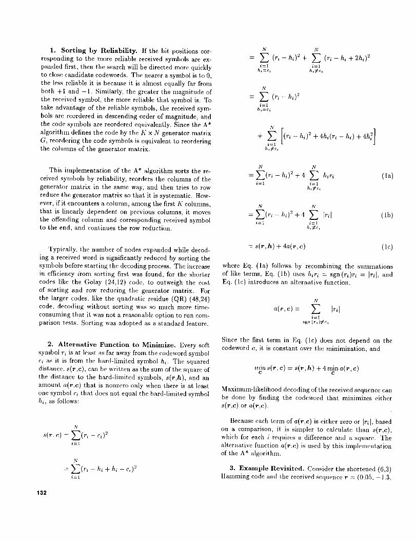
2. Alternative Function to Minimize. Every softsymbol ri is at least as far away from the codeword symbol
ci as it is from the hard-limited symbol hi. The squared
distance, s(r,c), can be written as the sum of the square of
the distance to the hard-limited symbols, s(r,h), and an
amount a(r,c) that is nonzero only when there is at least
one symbol ci that does not equal the hard-limited symbolh/, as follows:
N
s(r, C) ---- E(ri -- Ci) 2
i=1
N
= E(ri -- hi +hi-ci) 2
i=1
N N
E (ri-hi) 2+ E (ri-hi+2hi) 2i----1 i=1
ht-_ct h,_c,
N
= h,)2i=1
hi'el
N
i=1
h,#c,
N N
=Z (ri-hi)2+4 E hirii=1 i:1
h,#c.
(la)
N N
: h,)2+ 4 I,',1i=1 i=1
h,#c,
(lb)
: s(r,h) + 4a(r,c) (lc)
where Eq. (la) follows by recombining the summations
of like terms, Eq. (lb) uses hiri = sgn (r,)ri -- Iril, and
Eq. (lc) introduces an alternative function,
N
.(r,c)= Ei=I
sgn (r,)¢c,
Since the first term in Eq. (lc) does not depend on thecodeword c, it is constant over the minimization, and
rain s(r, c) = s(r, h) + 4 min a(r, c)C C
Maximum-likelihood decoding of the received sequence canbe done by finding the codeword that minimizes either
s(r,c) or a(r,c).
Because each term of a(r,c) is either zero or Iril, based
on a comparison, it is simpler to calculate than s(r,c),which for each i requires a difference and a square. The
alternative function a(r,c) is used by this implementationof the A* algorithm.
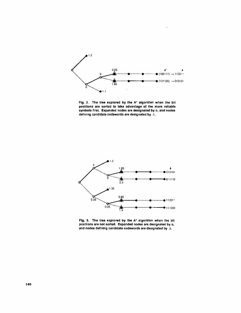
3. Example Revisited. Consider the shortened (6,3)
Hamming code and the received sequence r = (0.05, -1.3,
132

1.1, 0.8, -0.25, 0.6). Reordering tile received vector by,
magnitude gives r' = (-1.a, 1.1, 0.8, 0.6, -0.25, 0.05).Tile reordered generator matrix in systematic form is
i 0 0 l 1 l)[ 0 1 1 0
0 1 0 1 1
and a binary codeword b in the original code corresponds
to a sorted eodeword 5. Figure 2 shows the tree explored
by the A* algorithm when the sorted code is used. Eachnode is labeled with the value at that node of.the heuristic
flmction using the alternative function. Tile 3 expanded
nodes are each designated by a %'; the 2 candidate code-
words are each designated by a "A"; and tile 12 edges ex-
plored are the edges of tile tree that are shown. The nodeswith paths 0, 11, and 101 are dropped from the list whenthe candidate word, with alternative function 0.65, is put,
on the list. Tile search promptly t.erminates because the
top node on tile list. defines a candidate codeword, namely
b' = 100111. Unshuffling b' gives the maximun>likelihooddecoded codeword to be b = 110011. For comparison,
Fig. 3 shows the larger tree explored by the algorithm when
the symbols are not sorted.
C. Verification of the Decoder
The decoding results of the A* algorithm were com-
pared to the results of two exhaustive search decoder im-
plementations. The (24,12) Golay code was used for thistest since it has only 212 = 4006 codewords, making it fea-
sible to get timely results from an exhaustive search de-coder. First, the software decoded the received sequences
using both A* and exhaustive search, and compared theresults internally. Second, a couple hundred received se-
quences were decoded by both the A* software and anindependent exhaustive search decoder written in APL.The results showed that both exhaustive search and A*
decoders decoded the same noisy vectors t.o the same code-
words.
The software to implement the A* algorithm has beenwritten in C and run on several Sun platforms. Since in-
tegers on these processors are a2 bit.s long, the software
to implement the A* algorithm has been constrained tolinear codes with 64 or fewer bits per codeword by' using
two 32-bit iutegers for each codeword. Because of this
implementation detail, it. was important to confirm thatthe A* software properly' decodes codes longer than length
32. Most interesting codes with lengths over a2 bits take
a prohibitively long time to decode exhaustively. A testcode with length N greater than 32 and one with more
than 32 information bits were devised so they could be
readily decoded by other means. The code with length
greater than 32 was created by repeating the parity bits of
tile Golay (24,12) code. This formed a (36,12) code thatwas no more difficult to exhaustively decode than was the
Golly (24,12) code. After debugging and testing, the de-coder decoded 500 codewords consistent with the exhaus-
tive decoder results. Next, a simple (34,33) code, consist-
ing of 33 informatiou bits and 1 overall parity bit,, wastested on 200 noisy received words. This code was se-
lected because a maximum-likelihood decoder is easy to
write, and an APL program was used to veri_' that the200 test, words decoded consistently.
D. Operational Details
To analyze the performance of either the algorithm or
a code, data are taken by running the software with differ-
ent input paranieters. For a giwm run, tile software takes
as input the generator matrix for the code, the SNR, theseed for tile random number generator, and the number of
words to decode. It. returns the aw, rage number of nodes
expanded, the average number of candidate codewords,and the number of word errors that occurred. Somet.imes
a system call from inside the program was used to providethe amount of cenl.ral processing unit (CPU) time con-
sumed during a run. These decoding runs rauged in sizefrom hnndreds t.o tens of thousands of decoded received
sequences. The codes that have been examined includea Bose (?haudhuri-Ilocquenghem (FICtt) (63,56) code, a
quadratic residue (48,24) code, a (;oily (24,12) code, aBCH (31,10) code, and a Reed Muller (32,16) code. The
data from multiple runs are combined careflllly to give the
results in the following sections.
III. Algorithm Performance
The intricacy of the A* algorit.hnl makes it difficult t.odescribe the number of calculations necessary t.o decode
a receiw_d sequence, l_ossit)le measures of the number ofcalculations describe the search size for the A* algorithmand include the number of candidate codewords, the nun>
bet of expanded nodes, and the number of edges searchedin the tree. The number of edges K in the search tree is
given by
E = 2X + (N -/_)(:
where X is the number of nodes expanded including the
root and (7 is the number of candidate codewords. Be-
cause the search size for l.he A* algorithm varies from one
133

received sequence to the next, the averages of these num-
bers over many received sequences are used for compari-
son. Section III.A explains simulation timing results thatshow that the search size and the time to decode are re-
[at.ed linearly. Section III.B shows how the average size
of the A* search tree depends on tile signal-to-noise ra-tio. Section III.C introduces other maximum-likelihood
decoders that are used for comparisons in Section III.D.
A. Time to Decode Versus Search Size
The average amount of time it takes to decode received
sequences retlects both the computational overhead for
each sequence decoded and the computations for each part
of the search tree. Analyzing the time to decode requires
that all of the timing data be taken on the same computerand that the accuracy of the timing data be sufficient to
perform comparisons. Tile system call used to generatethe timing information for a run was accurate to within
a second, which is too coarse to study data on individual
decoded sequences, but sufficient for data on ensembles of
decoded sequences.
The relationship between the indicators of search size
introduced earlier and decoding time may be observed in
the data from many runs for the quadratic residue (48,24)
code ou a Spare 10 Model 30 workstation. Tile averagedecoding times versus the average numbers of candidate
codewords and expanded nodes are shown in Fig. 4, along
with a weighted linear fit I to the data. Although the data
display a small amount of statistical variability, the time
to decode displays a nearly linear relationship to the indi-cators o1"search size.
The relatiotlshil) hetween the average numbers of ex-
panded nodes and candidate codewords for the (48,24)code in l"ig. 5 is well described as linear.
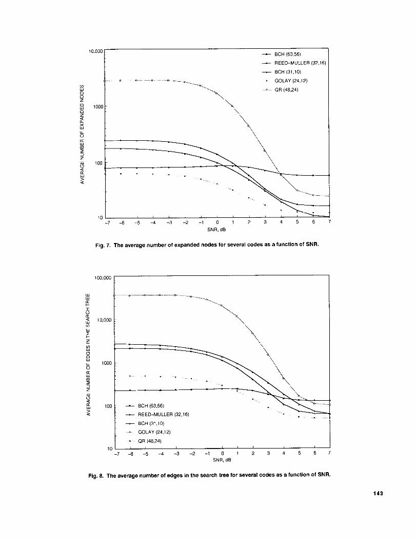
B. Search Size Versus SNR
The average size of the tree that the A* algorithmsearches is a function of the SNR for the received se-
quonces. For each of the codes studied, the average nun>bers of candidate codewords, expanded nodes, and search
tree edges are shown versus SNR in Figs. 6, 7, and 8,
resl>ectiw'ly. The total numt>er of sequences decoded foreach point in these figures is shown in Table 2.
Not surl>rismgly , for extremely high SNR, the A* algo-
rithm typically finds only two candidate words, along the
1 rl,he nunlber of dectMed words in each run was included in the linefitting process t_) account for the variati,m in accuracy bctwee.n<{ala fro]n large &lid small l'l.lllS.
way expands K nodes, and therefore has a search tree with
.E = 2K + 2(N - K) = 2N edges.
For low SNR, the soft symbols are predoininantly noise,but the A* algorithm still expands a mere fraction of the
nodes in the tree, especially as it bases early decisions on
the symbols that contribute most to the final choice. Fig-
ures 6 and 7 show that simulation data of the averagenumbers of candidate words and expanded nodes are al-most constant for SNRs below -4 dB. Since the number
of edges is calculated from the number of nodes and can-
didate words, the average number of edges also levels offfor low SNRs, as seen in Fig. 8.
The algorithm was also tested for each code with nosignal at all, i.e., an SNR of -,30. Table 3 shows that for
each code the average number of expanded nodes and the
average number of candidate words during A* decodingwere comparable to the numbers for SNRs below -4 dB.
It also shows the number of words decoded to obtain these
averages.
C. Other Maximum-Likelihood Decoders
Many other maximum-likelihood soft-decision decodingalgorithms use a fixed number of calculations to decode
any received sequence, independent of the SNR.
1. Exhaustive Search and Full Tree Search. An
exhaustive search decoder calculates the distance between
the received sequence and each codeword in the code in-
dividually, and returns the codeword with the minimum
distance. For an (N, Ix') block (:ode, an exhaustive searchtechnique computes the distances from the received se-
quence to all 2K codewords. If exhaustive search is cast
in terms of a graph with one edge for each bit in each
codeword, the number of edges for an exhaustive search isN21";, independent of the SNR.
A slightly more efficient technique to compute the dis-tances to all the codewords is to use the full code tree.
Here the squared distance from the received sequence to a
codeword, at a leaf, is the sum along the path to that leaf
of the squared distances from each received symbol to the
symbol associated with each edge. For an (N, K) code, thenumber of edges in the fidl tree is 2K+I - 2 + (N- K)2 K.
This technique checks all 2K leaves but has fewer edgesthan an exhaustive search.
2. Viterbi Decoding of Block Codes. To applysoft-decision Viterbi <tecoding to a block code, the code is
represented as a trellis. Wolf [6] and Massey [7] introduce
a minimal code trellis for block codes. McEliece [8] shows
134
a simple technique for constructing the minimal trellis for
a given code, and also shows that it is optimal for Viterbi
decoding complexity. A Viterbi decoder for a code on atrellis uses a constant number of calculations and com-
parisons independent of signal-to-noise ratio. The Viterbi
decoding complexity for a given trellis for a given code can
be measured by the number of edges in the trellis.
Less is known about the best trellises for the quadratic
residue (48,24) code. A worst-case permutation produces
a minimal trellis with 226-4 = 67,108,860 edges. A better
permutation results in a minimal trellis with 925,692 edges.
The A* algorithm search tree has on average 34,429 edges
when no signal is present.
An (N, K) code has a minimal trellis that can be con-
structed from the generator matrix. Different permuta-
tions of a code may have different minimal trellises. There
are codes, such as cyclic codes, for which the minimal trel-
lis has the most edges compared with the minimal trellisesfor other permutations of the code. The permutation that
gives the most edges in the minimal trellis is the worstpermutation of the code. The number of edges in the min-
imal trellis for the worst permutations is no more than
2M+2-4+2M(N- 2M) where M = rain (K,N- K + 1).
Other permutations give smaller minimal trellises.
D. Comparisons
The search size for the A* algorithm depends on the
received sequence, and the average search size depends
on the SNR. The averages found with no signal present
are used for comparison with the maximum-likelihood de-coders that use a fixed number of calculations.
Table 4 shows the number of edges used for an exhaus-tive search for each code and for the full code tree, both of
which are greater than the average number of edges in the
A* search tree shown for the case of no signal in Table 3.
The average number of edges in the search tree for the
A* algorithm is presented for comparison to the number
of edges in the trellis for Viterbi decoders. Table 4 also
shows the number of edges in some special trellises for thecodes where the numbers are known or bounds have been
calculated.
IV. Future Enhancements
There are several elements affecting the etticiency of the
software, including the initial computations to set up the
search, the size of the search, and the number of compu-
tations for each part of the search. With greater under-
standing of the algorithm come more ideas for improvingthe software to reduce at least one of these elements. Ei-
ther using the minimum distance of the code to determine
if the search can be successfully terminated before the list
is exhausted or improving the heuristic function will re-
duce the search size. Ideas like reducing the complexity
of sorting the received symbols for each decoding will trim
the number of initial setup computations, but will increase
the search size by an undetermined amount.
A. Escaping When a Candidate Is Definitely Closest
If the angle hetween the received word and a candi-
date codeword, as viewed from the origin, is less than half
the mininmm angle between any two codewords, then thatcandidate codeword is the closest one to the received word.
One of the suggestions in [2] is to calculate the angle be-tween the received word and each candidate codeword as
it is found. If this angle indicates that the candidate is
the closest codeword, then declare that the decoding is
complete, and exit the algorithm.
This feature has not been implemented at this writing,but is expected to reduce the size of the tree searched.
Consider the Golay (24,12) code. An exhaustive search
explores (24)212 = 98,304 edges. The full tree has 2 la
- 2 + (12)212 = 57,342 edges. The number of edges inthe minimal trellis for the worst-case permutation of the
Golay (24, 12) code is 214 - 4 = 16,380. The number of
edges in the minimal trellis for the best permutation of
the Golay code is 3580 [8]. By using enhancements ona certain trellis for the Golay code, Forney [9, p. 1183]
reduces the number of binary operations of a decoder to
1351. This decoder is mentioned as interesting, but the
number of binary operations is not directly comparable to
edge counts for the A* algorithm. Note that at low SNRsthe A* algorithm on average expands 62 nodes, checks 29
candidate codewords, and has a search tree with 4B9 edges.
B. Improving the Heuristic Function
Each parity bit is a linear function of a subset of the
information bits. If a node in the tree is deep enough to
specify all the information bits for a particular parity bit,
then any codeword passing through that node will have the
same value for that parity bit. The heuristic function could
use this parity bit to improve the distance underestimate
for all nodes at that depth, and thus reduce the size of the
tree searched by the algorithm.
C. Sorting Fewer Symbols
To simplify the sorting of symbols by reliability and the
necessary row reductions to the generator matrix, it may
135

be beneficial to sort only the information symbols or to
sort. only a few of the most reliable symbols.
Sorting only the infornmtion symbols ill tile received
word greatly simplifies the production of a systematic
generator matrix for the reordered code bits. Since thecolumns corresponding to information bits are columns of
an identity matrix, they are linearly independent, and ex-
changing rows is all it. takes to return the generator matrixto systematic form. Thus, the row reduction portion of the
algorithm is simplified.
Another possibility for simplifying sorting is to reorder
only the t_ most reliable linearly independent symbols and
not to reorder the rest. In such a design, there are no more
than N!/(N - n)! reorderings of the columns, and, hence,
this many systematic generator matrices. For small values
of i, such as 1 or 2, it may be acceptable to store and
retrieve systematic generator matrices for each of these
reorderings.
V, Code Performance
The A* algorithm that we have implemented has beenvery usefld for simulating code performance. Figure 9
shows the probability of word error versus SNR for the
BCH (63,56), Reed Muller (a2,16), BCH (31,10), Golay
(24,12), and quadratic residue (48,24) codes. The errorbars are one standard deviation of an average of m inde-
pendent Bernoulli trials. Specifically, the estimated stan-
dard deviation is cr = k/p(1 -p)/m, where p is the esti-mate of the probability of word error at a given SNR, and
m is the number of decodings done at that SNR.
VI. Conclusions
The application of the A* algorithm to maximum-
likelihood soft-decision decoding allows for efficient sim-
ulation of code performance. The A* algorithm finds thecodeword that maximizes the likelihood of the received
word given the codeword. This is equivalent to minimizingeither the Euclidean distance between the received word
and a codeword or the alternative function described in
Section II.B.2. The use of a heuristic flmction constrains
the search to only a subtree of the code's finite binary tree.
The heuristic flmction underestimates the function beingminimized in order to ensure that the subtree contains the
optimal path.
The size of the tree searched by the A* algorithm, as
described by the numbers of nodes expanded, candidate
words, and edges, is a good indicator of the complexity for
decoding that received sequence. Since the search size de-
pends on the received sequence, the average search size as
a function of signal-to-noise ratio is used for comparison.The search tree is smallest for a high SNR, where the algo-
rithm goes straight to the maximum-likelihood codeword,
and larger at a low SNR, where tile searched portion of thetree is still much smaller than the full code tree. At a low
SNR, the average size of the A* search tree is also smaller
than the fixed trellis size of a good Viterbi decoder.
For research applications, simulations using this imple-
mentation can provide data on code performance, such
as word error rate, for comparisons to theoretical results,
such as bounds, and for testing other predictors of code
performance.
Acknowledgments
The authors would like to thank A. Kiely, R. McEliece, and F. Pollara for many
helpful discussions.
136

References
[1] N. J. Nilsson, Principles of Artificial Intelligence, Palo Alto, California: Tioga
Publishing Co., 1980.
[2] Y. S. Han, C. R. P. Bartmann, and C.-C. Chen, Efficient Maximum-LikelihoodSoft-Decision Decoding of Linear Block Codes Using Algorithm A *, Technical
Report SU-CIS-91-42, School of Computer and Information Science, Syracuse
University, Syracuse, New York, December 1991.
[3] Y. S. Han and C. R. P. Hartmann, Designing Efficient Maximum-Likelihood
Soft-Decision Decoding Algorithms for Linear Block Codes Using Algorithm A *,
Technical Report SU-CIS-92-10, School of Computer and Information Science,
Syracuse University, Syracuse, New York, June 1992.
[4] Y. S. Han, C. R. P. Hartmann, and C.-C. Chen, "Efficient Priority-First SearchMaximum-Likelihood Soft-Decision Decoding of Linear Block Codes," IEEE
Transactions on Information Theory, vol. 39, no. 5, pp. 1514 1523, September
1993.
[5] S. Benedetto, E. Biglieri, and V. Castellani, Digital Transmission Theory, En-
glewood Cliffs, New Jersey: Prentice Hall, Inc., 1987.
[6] J. K. Wolf, "Efficient Maximum Likelihood Decoding of Linear Block CodesUsing a Trellis," IEEE Transactions on Information Theory, vol. IT-24, no. 1,
pp. 76-80, January 1978.
[7] J. L. Massey, "Foundations and Methods of Channel Coding," Proceedings
of the International Conference on Information Theory and Systems, NTG-Fachberichte vol. 65, Berlin, pp. 148 157, September 18-20,1978.
[8] R. J. McEliece, "The Viterbi Decoding Complexity of Linear Block Codes," to
be presented at IEEE ISIT'94, Trondheim, Norway, June 1994.
[9] G. D. Forney, Jr., "Coset Codes -- Part II: Binary Lattices and Related Codes,"IEEE Transactions on Information Theory, vol. IT-34, no. 5, pp. 1152 1187,
September 1988.
Table 1. Information sequences and the corresponding binary and
transmitted codewords for the (6,3) shortened Hamming code.
Information Binary _I'ransmit t ed
sequence ar codeword b codeword c
000 000000 1 1 1 1 1 1
001 001011 1 1-1 1 -1 -1
010 010 l 01 1 --1 1 --1 1 -I
011 011110 1 -1 --1 -1 -1 1
1 O0 1 O0110 -1 1 1 -1 -1 1
101 101101 -1 I -1 -1 1 -1
110 110011 -1 --1 1 1 -1 -1
111 111000 -1 --1 --1 1 1 1
137

SNR, dB
Table 2. The number of codewords decoded and used to generate
Figs. 6 through 9.
BCIt QR Golay Reed-Muller BCH
(31,101 (48,24) (24,121 (32,16) (63,56)
-- 7 40,000 6200 6400 6400 61 O0
-- 6 40,000 6200 6400 6400 6100
-- 5 40,000 6200 6400 6400 5900
--4 40,000 6200 6400 6400 5900
-3 40,000 6200 6400 6400 5900
-- 2 642,100 47,400 58,900 6400 33,300
- 1 923,200 70,600 71,700 19,200 57,200
0 1,204,000 83,500 84,500 32,000 83,700
1 1,483,000 207,900 385,000 279,300 279,600
2 3,362,100 409,800 465,000 359,100 468,900
3 5,014,000 1,042,500 1,102,500 995,000 1,036,000
4 6,212,500 1,571,000 2,113,000 1,200,000 1,256,000
5 7,418,000 2,472,500 6,055,000 1,400,000 1,476,000
6 21,242,000 8,048,000 16,330,000 7,200,000 6,512,000
7 12,400,000 8,337,000 8,400,000 8,400,000 7,5,17,0(/0
Table 3. The number of codewords decoded at an SNR of negative infinity, and the average
numbers of expanded nodes, candidate codewords, and edges in the search tree for the A*
algorithm.
A* results at SNR of negative infinityBCH QR Golay Reed-Muller BC[t
(31,10) (48,24) (24,12) (32,16) (63,56)
Number of decoded words 89,400 29,900 90,000 59,600 35,600
Average number of expanded nodes 181.16 2705.54 62.45 244.66 79.59
Average number of candidate codewords 120.96 1209.07 28.65 113.34 12.28
Average number of edges in search tree 2902.56 34,428.71 468.68 2302.77 245.12
138
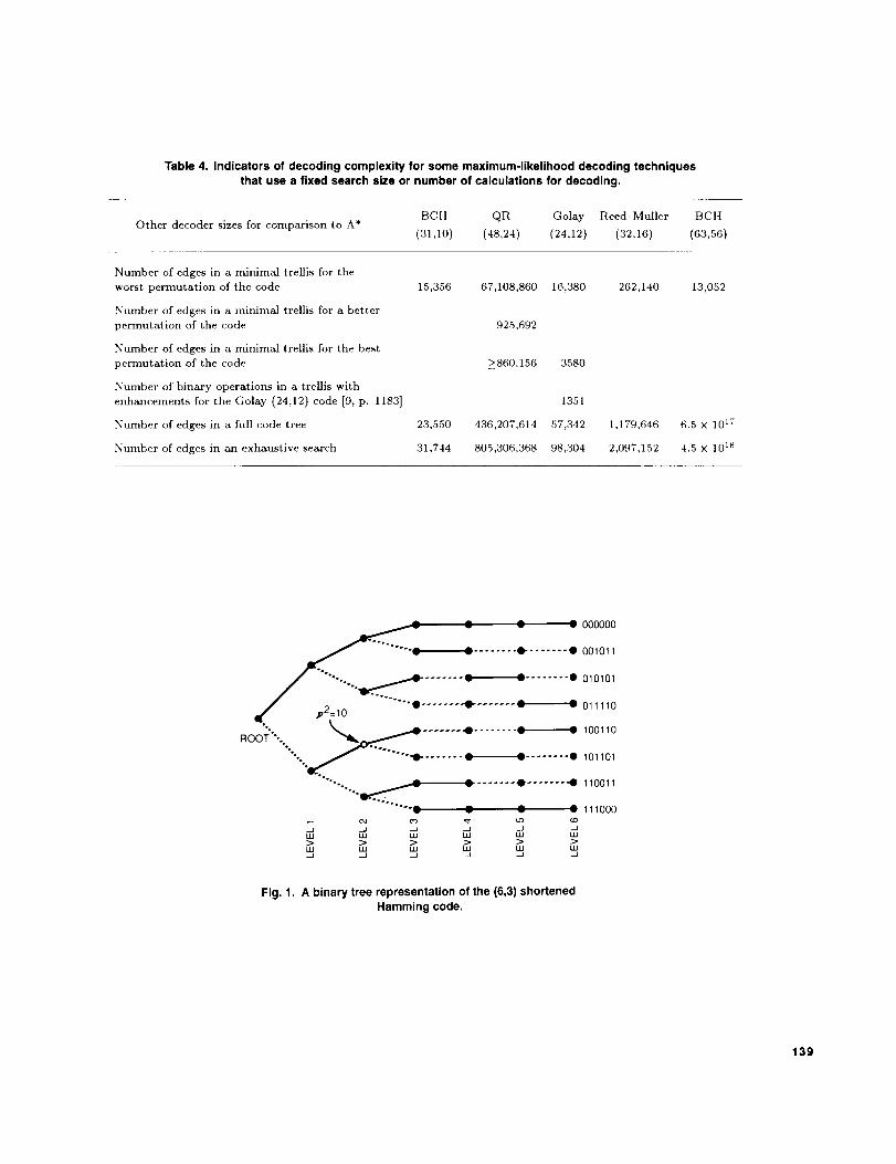
Table4.Indicatorsofdecodingcomplexityforsomemaximum-likelihooddecodingtechniquesthatuseafixedsearchsizeornumberofcalculationsfordecoding.
Other decoder sizes for comparison to A*BCH QR Golay Reed-Muller
(31,10) (48,24) (24,12) (32,16)
BCH
(63,56)
Number of edges in a minimal trellis for the
worst permutation of the code 15,356
Number of edges in a minimal trellis for a better
permutation of the code
N,maber of edges in a minimal trellis for the best
permutation of the code
Number of binary operations in a trellis with
enhancements for the Golay (24,12) code [9, p. 1183]
Number of edges in a full code tree 23,550
Number of edges in an exhaustive search 31,744
67,108,860 16,380
925,692
>860,156 3580
1351
436,207,614 57,342
805,306,368 98,304
262,140
1,179,646
2,097,152
13,052
6.5 x 10¹⁷
4.5 × 10¹⁸
_ 00000o
.......... _. : ........ •- ....... • 001011
""'*-.. " ...... : : ........ • 010101
011110
.......°........: -,oo,,o",. J ..... "0" ....... ¢ _ ........ • 101101
e¢,
"'+--+..+._ ....... • ....... 4 110011111000
W W W UJ
Fig. 1. A binary tree representation of the (6,3) shortened
Hamming code.
139
jl.3 0_5 b' &
°°eet
•, _- ...... -t- ....... • ....... -0(100111) -_ 110011
"'' _r ....... ; " ; (101100)-_ 010101
0 °"'*.
°"-0 1.1
Fig. 2. The tree explored by the A* algorithm when the bit
positions are sorted to take advantage of the more reliable
symbols first. Expanded nodes are designated by o, and nodes
defining candidate codewords are designated by t_.
0_1.3
......... "...... ; ; ....... -0010101
/ 0 ...... °_. ....... .0 ........ ; ;011110
¢E, 2.5%%
°_,_ ; ; ; 11 1000O.05
1.4
Fig. 3. The tree explored by the A* algorithm when the bit
positions are not sorted. Expanded nodes are designated by o,
and nodes defining candidate codewords are designated by A.
140

45O
400
350
E 300wa0(_)
250
O
--200
w
<
_ 150
(a)
100
0 t 1i i L
0 200
• •
,P
• -2 dB
• -1 dB
• 0dB
t 1 dB
o 2dB
o 3 dB
4dB
<> 5dB
a LINEAR FIT
] i i i I
400 600 800 1000 1200 1400
AVERAGE NUMBER OF CANDIDATE CODEWORDS
450
400
350
E 300wDOo
250
0
u.I2oo
w
150><
100
5O
(b)
5OO
$
mm
• -2 dB
• -1 dB
• 0 dB
1 dB
[] 2dB
O 3dB
4dB
,o. 5dB
m LINEAR FIT
1000 1500 2000 2500 3000
AVERAGE NUMBER OF EXPANDED NODES
Fig. 4. Scatter plots of average CPU time per decoded word versus (a) average number ofcandidate codewords per decoded word and (b) average number of expanded nodes per decoded
word, for the quadratic residue (48,24) code on a Sparc 10 Model 30 workstation.
141

1400
1200
0
0
1000DOOw
<o 800
z<o
600
w
z
400
2O0
0 , , , , I I
500 1000 1500 2000
AVERAGE NUMBER OF EXPANDED NODES
• -2dB
• -1 dB
• 0dB
_. 1 dB
o 2dB
o 3dB
4dB
o 5dB
• 6dB
• LINEAR FIT
I ,2500 1000
Fig. 5. A scatter plot of the average number of candidate codewords versus the average number
of expanded nodes for the quadratic residue (48,24) code, shown with a weighted linear fit.
142
10.000
D
OlOO0
woo
w
a
z
100
w
zw
_ 10w
BCH (63,56)
REED-MULLER (32,16)
BCH (31,10)
- GOLAY (24,12)
....... QR (48,24)
I 15 14 13 i2 11 i J I _ I i i1 -7 -6 ..... 0 1 2 3 4 5 6
SNR, dB
Fig. 6. The average number of candidate codewords for several codes as a function of SNR.
(,ouJr"-,OzowQZ,<(I.xuJu_0n"uJrn=s
ZuJ©
n-w
<
10,000
lOOO
1DO
to
BCH (63,56)
REED-MULLER (32,16)
-- BCH (31,10)
.... GOLAY (24,12)
........QR (48,24)
-7 -6
"%\.\._
\N
N
V mI
-5 -4 -3 -2 -1 0 1 2 3 4 5 6
SNR, dB
Fig. 7. The average number of expanded nodes for several codes as a function of SNRo
100,000
ww
IO
< 10,000w
wI
Z
w
aw
I000
w
zw
<E 100w><
IO-7
o- ........
""'X,,
\\
BCH (63,56) . .......
REED-MULLER (32,16) - ....
-- BCH (31,10)
• GOLAY (24,12)
......... QR (48,24)
i i i i L i i i i i J i i
-6 -5 -4 -3 -2 -1 0 1 2 3 4 5 6 7
SNR, dB
Fig. 8. The average number of edges in the search tree for several codes as a function of SNR.
143

I ×I0 0
1 x 10 -1
1 xlO -2
1 xlO -3
I xlO -4
1 xlO -5
\
\\
\\\\\\\\b
\
\\
\\\
L
1 xlO -6
lx1_ 7
t BCH (63,56)
REED-MULLER (32,16)
BCH (31.10)
GOLAY (24,12)
"Et"" QR (48,24)
I I I r I I I I I I r I I
-7 -6 -5 -4 -3 -2 - 1 0 1 2 3 4 5 6
SNR, dB
Fig. 9. Probability of word error versus SNR for the BCH (63,56), Reed-Muller (32,16), BCH (31,10),
Golay (24,12), and quadratic residue (48,24) codes. The error bars are _+0, one standard deviation.
144