PHYSICAL REVIEW E 101, 012106 (2020)

Maximum entropy approach to reliability

Yi-Mu Du,1 Yu-Han Ma,2 Yuan-Fa Wei,3 Xuefei Guan,1,* and C. P. Sun1,2,†

1Graduate School of China Academy of Engineering Physics, Beijing 100193, China2Beijing Computational Science Research Center, Beijing 100193, China

3Institute of Systems Engineering, China Academy of Engineering Physics, Mianyang 621999, China

(Received 28 September 2019; published 3 January 2020)

The aging process is a common phenomenon in engineering, biological, and physical systems. The hazardrate function, which characterizes the aging process, is a fundamental quantity in the disciplines of reliability,failure, and risk analysis. However, it is difficult to determine the entire hazard function accurately with limitedobservation data when the degradation mechanism is not fully understood. Inspired by the seminal workpioneered by Jaynes [Phys. Rev. 106, 620 (1956)], this study develops an approach based on the principleof maximum entropy. In particular, the time-dependent hazard rate function can be established using limitedobservation data in a rational manner. It is shown that the developed approach is capable of constructing andinterpreting many typical hazard rate curves observed in practice, such as the bathtub curve, the upside downbathtub, and so on. The developed approach is applied to model a classical single function system and a numericalexample is used to demonstrate the method. In addition its extension to a more general multifunction system ispresented. Depending on the interaction between different functions of the system, two cases, namely reducibleand irreducible, are discussed in detail. A multifunction electrical system is used for demonstration.

DOI: 10.1103/PhysRevE.101.012106

I. INTRODUCTION

The aging process is a common phenomenon in manyengineering, biological, and physical systems. Modeling theaging process is of critical importance for the evaluation ofreliability, availability, and safety of a system, and thus iswidely concerning. However, it is difficult to describe theaging process microscopically due to its inherent complex andstochastic nature. Consequently the lifetime of a componentor system, as the final outcome of the aging process, is alsorandom. The hazard rate function characterizing the time-dependent nature of the aging process plays an importantrole in reliability engineering [1]. Knowing the hazard ratefunction allows for prediction of the lifetime distribution andtherefore the failure probability can be evaluated. Early andsystematical attempts in construction of the hazard functioncan be traced back to the reliability study of military radarsystems [2]. The statistical analysis of component life testingdata has since become an engineering practice to estimate thehazard rate function. The bathtub shape of the hazard ratefunction is then widely observed and the mechanism of sucha shape is empirically explained.

To describe the above mentioned concept in detail, con-sider a single function system with an uncertain lifetime Tas a random variable. The survival function, F (t ), is de-fined as the probability that the lifetime T is greater than t ,i.e., F (t ) = Pr(T � t ), where t ∈ (0,+∞). The correspond-ing probability density function (PDF) for lifetime T = t isobtained as p(t ) ≡ −dF (t )/dt with a normalizing constant

*xfguan@gscaep.ac.cn†cpsun@csrc.ac.cn

∫ ∞0 p(t )dt = F (0) − F (∞) = 1. The hazard rate function

x(t ) is then defined as

x(t ) ≡ − 1

F (t )

dF (t )

dt= p(t )

F (t ). (1)

The hazard rate is the failure rate of the system at time tconditioning on the system at t is still functioning. Empiricalevidences show that for a number of systems, the hazard ratefunction exhibits the so-called bathtub shape or U shape (thesolid curve shown in Fig. 2). The earliest bathtub shapedhazard rate function appears in an actuarial life-table analysisin 1693 [3,4]. The bathtub shape of the hazard rate functionimplies that the failure mechanism of the system may be di-vided into three phases: the infant mortality, random failures,and wear-out failures.

Although the bathtub shape of hazard rate functions iswidely observed in many realistic components and systems,the lack of underlying physical theory supporting the inter-pretation leads to some criticisms [4]. Moreover, the hazardrate functions that are not in bathtub shape are also observedin some biological systems [5] and electronic systems [6].Beside the areas of engineering science and biology, the agingprocesses (especially in materials) are also widely concernedin the area of material physics [7–14], including, but notbe limited to, the rupture of the fibrous materials [9,12],the cracking of heterogeneous material [10,13], and physicalaging of colloidal glass [14].

The perspectives on the aging problems may be differ-ent to engineers and physicists. The former usually focuseson the degradation of the functioning systems and lifetimedistributions. The latter concerns the physical and statisticallaws in aging processes. The physical aging usually means thedynamical relaxation of the systems [15–19]. The connections

2470-0045/2020/101(1)/012106(16) 012106-1 ©2020 American Physical Society

DU, MA, WEI, GUAN, AND SUN PHYSICAL REVIEW E 101, 012106 (2020)

between the aging processes in different areas are also signi-fied in, for example, Ref. [20] where a direct link between thebiological aging and the physical aging is established.

The hazard rate function is usually difficult to obtain dueto the lack of precise understanding of the physical mech-anism and the limitation of information access. Statisticalanalysis is one of the most common approaches to estimatethe hazard rate curves using lifetime testing data. A sufficientamount of lifetime data are required to ensure a reliableestimation of the hazard rate curve. A few methods havebeen reported to fit the hazard rate curves based on Weibulldistributions, Lindley distributions, exponential distributions,and its variants [21–23]. The modeling of the commonly seenbathtub shaped failure rate curve is reviewed in Ref. [24] andsome recent development regarding this topic is discussed inRefs. [25,26]. The performance of these methods relies onthe sufficiency of the experimental data and the choice ofdistributions. Another approach to construct the hazard ratefunction is based on modeling the physical mechanism of theaging process [7–9]. This approach can provide a clear phys-ical picture of the aging process and a close agreement withexperimental data is observed for relatively simple systems.For systems with complex aging mechanisms this approachis difficult to apply. Recently, entropy-based methods arealso reported to tackle the problems in the field of reliability[27–36]. In Refs. [27–29], the authors considered remaininglifetime and corresponding time-dependent residual entropy,and investigated the lifetime distributions to maximize theresidual entropy in several conditions.

Although many studies have been reported on estimationof the hazard rate curve, an approach built upon fundamentalprinciples of physics to construct the hazard rate function israrely seen. In addition, to the best of the authors’ knowledge,there is no analytical modeling work reported on multifunc-tion systems consisting of several individual components. Inview of this, the goal of this study is to develop an approachto reliability problems based on the fundamental principle ofmaximum entropy (MaxEnt), allowing for the construction ofthe hazard rate function in a rational manner given availabledata. This study extends the MaxEnt method to the time-dependent cases. The principle of MaxEnt and the least-actionprinciple is compared to formulate the equation of motionfor the most probable hazard rate, i.e., the Euler-Lagrangeequation. Another focus of this study is to reveal the under-lying connection between different shapes of the hazard rateand the information processing. Both the model-dependentand the data-dependent hazard rate shapes are investigated inthis study. In addition, the modeling of multifunction systemsconsisting of multiple individual components is made usingthe developed approach. A linear assumption is incorporatedto cope with the complexity introduced by multiple functionsin the system. Using the linear assumption, the hazard rate ofthe system can be represented as a multidimensional matrix.Depending on the interaction between each individual func-tion, two cases, namely the reducible one and the irreducibleone, are derived using the proposed method. It demonstratesa viable means for the bottom-up modeling of hazard ratefunctions of complex systems.

This paper is organized as follows. In Sec. II, the principleof MaxEnt is briefly reviewed. The variational technique is

applied to MaxEnt to formulate the dynamical equation of thehazard rate. The equation of motion is solved to obtain themost probable hazard rate function. In Sec. III, the modelingof the hazard rate function for single function systems ispresented. Using a double-moment constraint, the modelingproblem is recast to a MaxEnt inference problem. It is shownthat the resulting model is capable of producing three differentshapes of the hazard rate curves: the bathtub shape, theupside down bathtub shape, and the monotonically increasingshape. The data dependence of the shapes is demonstratedby using different model parameters. Furthermore, using aquadruple-moment constraint allows the resulting model toproduce other shapes of the hazard rate function. Numericalexperiments of a single-function electrical system is usedto validate the effectiveness of the method. In Sec. IV, themodeling of multifunction systems where the correlation isamong the components is presented. A two-lamp circuit isused to demonstrate the modeling of multifunction systems.Finally, conclusions are drawn in Sec. V.

II. MAXENT METHOD

A. Principle of maximum entropy (MaxEnt)

The concept of entropy was originally introduced by Clau-sius to identify the reversible and irreversible processes inthermodynamics. According to the view of Clausius, thesecond law of thermodynamics states that the entropy of athermal-isolation system never decreases. Boltzmann, then,associated the entropy to statistical quantities, laying out thefoundation of the modern statistical physics. Shannon [37]developed the information theory which is based on a quantitycalled Shannon entropy, S = −∑

i pi log pi, as a measureof information loss or the ignorance of an observer. Jaynes[38,39] combined the insights of both statistical physics andinformation theory, and established the fundamental logic ofprobabilistic inference. In his point of view, statistical physicsis only to do probabilistic inferences from limited informationbased on the principle of MaxEnt. Jaynes [40] later comparedthe MaxEnt method with other methods of inference, andpointed out that it is applicable to inference problems with awell-defined hypothesis space and noiseless incomplete data.

The principle of MaxEnt states that the most probabledistribution function is the one that maximizes the entropygiven testable information. A PDF p(t ) and its hazard ratefunction x(t ) relate to each other through

p(t ) = x(t ) exp

[−

∫ t

0x(t ′)dt ′

]. (2)

Note that Eq. (2) is just the solution to Eq. (1). Using Eq. (2),the entropy S for a given PDF p(t ) can be expressed as

S = −∫ ∞

0p(t ) ln p(t )dt

= −∫ ∞

0X exp(−X ) ln[X exp(−X )]dt, (3)

where X = ∫ t0 x(t ′)dt ′ and X = x(t ). The entropy in Eq. (3)

is called the differential entropy. A constant term ln(dt ) hasbeen neglected, and thus the term ln p(t ) has an abnormaldimension. In Eq. (3) the measure in integral is set to dt . In

012106-2

MAXIMUM ENTROPY APPROACH TO RELIABILITY PHYSICAL REVIEW E 101, 012106 (2020)

general, the measure should be properly chosen according tothe prior knowledge.

Experimental data can be encoded into pieces oftestable information using statistical moments of any observ-able time-dependent quantities gi(t ), i = 1, 2, . . ., i.e., gi =∫ ∞

0 p(t )gi(t )dt, i = 1, 2, . . .. To maximize the entropy basedon the testable information, the variational term of the entropycan be used,

δS = δ

(−

∫ ∞

0p(t ) ln p(t )dt − α

∫ ∞

0p(t )dt

−∑

i

βi

∫ ∞

0gi(t )p(t )dt

)

= − δ

(∫ ∞

0X exp(−X )

{ln[X exp(−X )]

+ α +∑

i

βigi(t )

}dt

)= 0, (4)

where α and βi, i = 1, 2, . . . are Lagrange multipliers.

B. Entropy as the action of hazard rate dynamics

The entropy in the above equation is the function of thetime dependent variable X = ∫ t

0 x(t ′)dt ′. To determine themost probable hazard rate one may adopt the variationalprinciple. In this sense the concept of MaxEnt is similar tothe least-action principle.

One can see that the quantity S = −S is similar to the ac-tion which governs the hazard rate dynamics. The “velocity”X which minimizes the action is the most probable hazardrate. We rewrite Eq. (4) in Lagrangian form explicitly to have

L[X, X , t] =X exp(−X )

{ln[X exp(−X )] + α +

∑i

βigi(t )

}.

(5)

To maximize the action, X satisfies the Euler-Lagrange equa-tion

d

dt

(∂L∂X

)− ∂L

∂X= 0, (6)

which is expressed explicitly as

X − X 2 + X∑

i

βigi(t ) = 0. (7)

The Lagrange multiplier α is related to the normalization anddoes not appear in the above equation because the function∫

X exp(−X )dt is nothing but a constant. This equation ofmotion governs the most probable hazard rate varying withtime. It should be noted that the constraints used for methoddevelopment are based on the lifetime statistics. The con-straints can be loosely seen as pieces of information encodingsome features over the entire lifespan. Therefore, the con-straints given above are not varying with time; therefore, theresulting Lagrange multipliers are not time-varying quantities.However when the constraints are time varying, the resultingLagrange multipliers will be time dependent. For example,the following constraint is time dependent and can result in

a time-dependent Lagrange multiplier,∫ ti+1

ti

p(t )dt = ci,

where i = 1, 2, . . ., ti < ti+1 for any i, and ci can be evaluatedfrom the empirical probability. It is worth mentioning thatthe method itself can deal with both the time-dependent andtime-independent constraints, as the underlying principle ofthe MaxEnt only provides a mechanism to process the givenconstraints as long as they are testable information.

Equation (5) should not be overlooked. Although on thesurface it appears as an algebraic manipulation, the signifi-cance of the established dynamics should be emphasized here.The hazard rate is originally a quantity in the statistical sense,and the dynamical equations are usually governed by theaction in physical theories. Equation (5) relates the hazard ratefunction to the dynamics of time-dependent aging processes.In this sense, the hazard rate becomes a bridge that links thestatistical and the dynamical aspects of aging processes. Inother words, the entropy here is not only the measure of un-certainty but also becomes the action that governs the hazardrate dynamics. This remark is established based solely on onefundamental physical principle, MaxEnt. Consequently, theMaxEnt method provides a natural and rational way to treatthe problem of reliability more physically.

C. Most probable hazard rate and distribution

Take the moments of lifetime as the constraints, i.e., gi =t i, and use the initial condition of gi(0) = 0 (i = 1, 2, . . .).Solve Eq. (7) with certain initial conditions to obtain

X = x0 exp( − ∑

i βigi)

1 − x0∫ t

0 exp( − ∑

i βigi)dt ′ , (8)

where X (0) = x0 is the initial hazard rate. The function inEq. (8) has a singularity point denoted by tmax with thefollowing condition:

x0

∫ tmax

0exp

(−

∑i

βigi

)dt ′ = 1. (9)

Note that the definition of hazard rates Eq. (1) shows thatthe hazard rates are always non-negative. The term X inEq. (8) is negative when t > tmax. It implies that only t � tmax

is allowable. This can be directly proved by verifying thenormalization condition. Substituting Eq. (8) into Eq. (2), fort � tmax, the PDF p(t ) becomes

p(t ) = x0 exp

(−

∑i

βigi

). (10)

Equation (9) is nothing but a normalization condition, andthe singularity tmax is the maximum lifetime. The detailedderivations and explanations of the maximum lifetime arepresented in Appendix A.

The above discussion shows that the physically allowablehazard rate is

x ≡ X ={

x0 exp(− ∑i βigi )

1−x0∫ t

0 exp(− ∑i βigi )dt ′ , 0 � t < tmax,

0, t � tmax,(11)

012106-3

DU, MA, WEI, GUAN, AND SUN PHYSICAL REVIEW E 101, 012106 (2020)

0x( )

x( τ )

maxx( t )x

tτ0 maxt

FIG. 1. Illustration of alternative additional constraints.x(0), x(tmax) are the alternative additional constraints at theboundary. One can, in general, use the hazard rate at an arbitrarytime x(τ ) to obtain the solution.

where X (0) = x0 is the initial hazard rate and tmax is themaximum lifetime. It follows from Eq. (2) that

p(t ) ={

x0 exp[ − ∑

i βigi(t )], 0 � t < tmax,

0, t > tmax.(12)

The normalization of p(t ) indicates that the maximum lifetimetmax is related to the initial hazard rate x0 through Eq. (9) andvice versa.

The hazard rate increases with time when t approaches tmax

given that tmax is finite. This feature plays an important rolein the bathtub shaped hazard rate function in the followingtwo aspects. First consider the initial hazard rate x0 and themoment gi are observed information, and the maximum life-time tmax and other features of the distribution are quantities tobe inferred. The following example illustrates this setting: themaximum lifetime of humans is the variable of interest to beinferred based on the information of infant mortality and theaverage lifetime. Conversely given that the maximum lifetimetmax and the moment gi are observed information, and theinitial hazard rate x(0) and other features of the distributionare quantities to be inferred, a different inference problem isformulated. For example, given the maximum lifetime tmax orthe average lifetime and its limit, an estimation on the initialhazard rate can be made. In general these local information,such as initial hazard rate x0 and the maximum lifetime tmax,serves as the boundary condition of hazard rate dynamics, andprovides the necessary constraint in solving the hazard ratefunction using MaxEnt. One can, in general, use the hazardrate at an arbitrary time to do the inference. However, theresults of the inference usually depend on the choice of suchadditional constraints, and are discussed in the next section.

The different choices of additional constraints are illus-trated in Fig. 1. It is worth mentioning that the most probabledistribution of the lifetime can be obtained from the hazardrate X by utilizing Eq. (2) or the equivalent Eq. (12). It canalso be determined directly using MaxEnt with necessaryconstraints such as the maximum lifetime or an initial hazardrate. It can be realized from Fig. 1 that the resulting distri-bution functions using the two considerations are equivalentif the observation error is omitted. The proof is presented in

Appendix A. This property is useful for the self-consistencytest of the method, which is discussed later.

III. SINGLE FUNCTION SYSTEMS

Following Eq. (1), the survival function F (t ) of a singlefunction system decreases with time as

dF

dt= −x(t )F (t ), (13)

where F (t ) = ∫ t0 p(t ′)dt ′ is a monotonically decreasing func-

tion and x(t ) � 0 is the hazard rate function.

A. Double-moment constraints

Recall that gi(t ), i = 1, 2, . . . denotes the random variableswhich can be observed from experiments. Usually only asmall number of samples are available in practical problems.In this case only the first order and second order momentsare reliable. Denote the first order and second order momentsas g1(t ) = t and g2(t ) = t2, respectively. Omitting the termt in x(t ) and representing x(0) as x0 only for simplicity, theequation of motion of the hazard rate becomes

x − x2 + x(β1 + 2β2t ) = 0, (14)

where β1 and β2 are the Lagrange multipliers for the firstand second order moments, respectively. Given the initialcondition x(0) = x0 > 0, the solution to Eq. (14) is

x =⎧⎨⎩

x0 exp(−β1t − β2t2)

1 − x0∫ t

0 exp(−β1t ′ − β2t ′2)dt ′ , 0 � t < tmax,

0, t � tmax.

(15)The normalization requires

x0

∫ tmax

0exp(−β1t − β2t2)dt = 1. (16)

Because tmax ∈ [0,∞) and exp(−β1t − β2t2) > 0, one has

x0

∫ ∞

0exp(−β1t − β2t2)dt � 1. (17)

This is the necessary and sufficient condition to guaranteethat the solution is physically viable. If the above conditionis violated, the resulting PDF cannot be normalized and thusis improper.

Conditions violating the inequality in Eq. (17) only occurwhen β2 > 0. The inequality always holds because the inte-gration

∫ ∞0 exp(−β1t − β2t2)dt is divergent when β2 < 0. In

particular, for β2 > 0, the equality implies the resulting PDFis a truncated Gaussian distribution.

Consider the triplet of (x0, β1, β2) which satisfies Eq. (17);the most probable hazard rate function x(t ) can yield threedifferent types of shapes. Table I presents the three possibleshapes and corresponding domains of parameters. The de-tailed derivations are presented in Appendix B. In the caseof β2 < 0, β1 > x0, the hazard rate functions are in bathtubshapes. In the case of β2 > 0, x0

∫ ∞0 exp(−β1t − β2t2)dt =

1, the hazard rate functions are in upside down bathtub shapes.The hazard rate functions are associated with truncatedGaussian distributions. In other physically viable cases, i.e.,

012106-4

MAXIMUM ENTROPY APPROACH TO RELIABILITY PHYSICAL REVIEW E 101, 012106 (2020)

TABLE I. Shapes of hazard-rate curves and the corresponding domains of parameters.

x0 � β1 x0 < β1

β2 < 0 monotonically increasing bathtub

β2 > 0 x0

∫ ∞0 exp(−β1t − β2t2)dt = 1 x0

∫ ∞0 exp(−β1t − β2t2)dt > 1

upside down bathtub monotonically increasing

β2 > 0, x0∫ ∞

0 exp(−β1t − β2t2)dt > 1, the hazard rate func-tions are monotonically increasing curves.

Figure 2 presents results of Eq. (14) with an initial con-dition x0 = 1 for illustration. For example, the hazard ratefunction associated with parameters β1 = −0.1 and β2 =1.5989 is a monotonically increasing curve, satisfying thecondition of β2 > 0 and x0

∫ ∞0 exp(−β1t − β2t2)dt > 1. The

parameters of the other two curves (the bathtub shape andthe upside down bathtub shape) also satisfy the conditionsyielding the two shapes. It should be noted that the quantitieswhich can directly be obtained from experimental data are notthe parameters of β1 and β2 but the moments of t and t2.

Note that the number of the possible types of shapesdepends on the constraints. The double-moment (the firstand second order moments) constraint can yield hazard ratefunctions in bathtub shapes, upside down bathtub shapes, andthe monotonically increasing curves. Figure 3 shows how theshape of the curves varies with the first order and second ordermoments. The numerical results show that if the point (t2, t )is located in the black region in Fig. 3, the resulting hazardrate function function exhibits a bathtub shape; otherwise, thehazard rate function is a monotonically increasing curve (inthe gray region). In this case the maximum lifetime is 1, i.e.,

0 0.5 1 1.5 2 2.5 30

0.5

1

1.5

2

2.5

3

3.5

4

4.5

5

t

x(t)

β1=−0.1, β

2=0.7979

β1=0, β

2=0.7979

β1=3.3, β

2=−1

FIG. 2. Hazard rate function x(t ) using a double-moment con-straint with different (β1, β2) parameters, showing three differentshapes. The initial hazard rate x0 is set to 1. The parameters asso-ciated with the three shapes are only for illustration purposes.

a finite quantity, and there is no hazard rate function in upsidedown bathtub shapes.

B. Quadruple-moment constraints

The analysis of the hazard rate function with a quadruple-moment constraint is similar to the previous one with adouble-moment constraint. Equation (7) implies that for aquadruple-moment constraint the equation of motion of thehazard rate function is written as

x − x2 + x(β1 + 2β2t + 3β3t2 + 4β4t3) = 0, (18)

where βi, i = 1, . . . , 4 are parameters that need to be solvedgiven the moment constraints. The resulting hazard rate func-tion x(t ) of the above equation has seven types of shapesat most. The proof is presented in Appendix B. Besides thethree types of shapes shown in the double-moment case, thequadruple-moment constraint is capable of generating W-and upside down W-, N- and upside down N-shaped curves.Figure 4 shows the additional possible four types of shapes ofthe hazard rate function allowed by Eq. (18). The parametersused in Fig. 4 are only for illustration purposes.

C. Illustration of MaxEnt: A circuit model

To demonstrate the performance of the MaxEnt method,the aging problem of an electrical system is presented in thissection. As shown in Fig. 5 the electrical system contains the

0 0.05 0.1 0.15 0.2

0.2

0.4

0.6

0.8

E(t2)

E(t

)

FIG. 3. Two regions of the hazard rate functions with differentfirst order moments E (t ) = t and second order moments E (t2) = t2.The maximum lifetime tmax is set to 1. The black region denotes thedomain generating monotonically increasing curves. The gray regiondenotes the domain generate bathtub shapes.

012106-5

DU, MA, WEI, GUAN, AND SUN PHYSICAL REVIEW E 101, 012106 (2020)

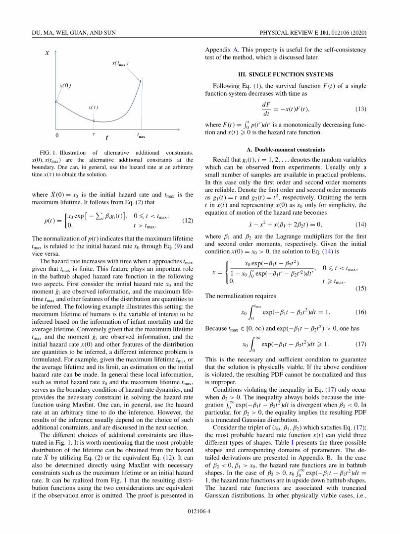
FIG. 4. Four additional shapes of the hazard rate function x(t )with a quadruple-moment constraint. The initial hazard rate x0 isset to 1. The parameters associated with the four shapes are onlyfor illustration purposes. These parameters satisfy the condition ofx0

∫ ∞0 exp(−β1t − β2t2 − β3t3 − β4t4)dt � 1.

battery source, the lamp and the conducting wire. The termE denotes the electromotive force of the source. The internalresistances of the lamp and the conducting wire are denotedby R and r, respectively. The resistance of the conductingwire increases due to the heat generation. For demonstrationpurposes, the regime where the temperature T is much higherthan the Debye temperature is considered, and the resistancer ∝ T [41]. The aging process due to the heat generation ofthe wire can be modeled with the thermodynamical consider-ation by

CdT

dt= λr

(E

R + r

)2

, (19)

where C is the heat capacity of the material of the conductingwire. The right hand side of the above equation denotes theremaining heat generated by the wire, and λ is a factor whichdepends on the heat conduction between the wire and theenvironment. With the high temperature approximation r ∝ T ,the above equation becomes

dr

dt= λr

(E

R + r

)2

, (20)

FIG. 5. Schematic of an electrical system consisting of thesource, the lamp, and the conducting wire.

where λ is the effective ratio parameter. This equation de-scribes the behavior of the time-dependent resistance r(t ).One can see that the efficiency η = R/(r + R) of the circuitdecreases in the aging process. The system failure criterionis defined as η � 50%. The aging process is stochasticwhen r(0) and λ are considered random variables. Numericalexperiments are made to generate data representing the actualobserved quantities. The initial resistance r(0) follows a PDFof p[r(0)] ∝ exp[−r(0)] in the interval [0.033,1]. The ratioterm λ is considered as a uniform distribution in [1,). Thefirst order and second order moments are used as constraints.To investigate the performance of the method under differentdistributions of r(0) and λ, different combinations of (,)are used. The Kolmogorov distance [42] between the esti-mated distribution pe and the simulated distributions ps isused as a measure to evaluate the performance of MaxEnt.The distance is defined as

ε =∫

dt1

2|pe(t ) − ps(t )|. (21)

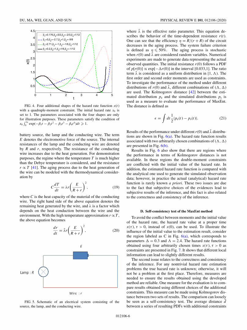
Results of the performance under different r(0) and λ distribu-tions are shown in Fig. 6(a). The hazard rate function resultsassociated with two arbitrarily chosen combinations of (,)are presented in Fig. 6(b).

Results in Fig. 6 also show that there are regions wherethe performance in terms of Kolmogorov distances is notavailable. In these regions the double-moment constraintsare conflicted with the initial value of the hazard rate. Inaddition, the estimated hazard rate function is compared withthe analytical one used to generate the simulated observationdata; however, in practice the actual (analytical) hazard ratefunction is rarely known a priori. These two issues are dueto the fact that subjective choices of the evidences lead tosubjective results of the inference, and this fact is also relatedto the correctness and consistency of the inference.

D. Self-consistency test of the MaxEnt method

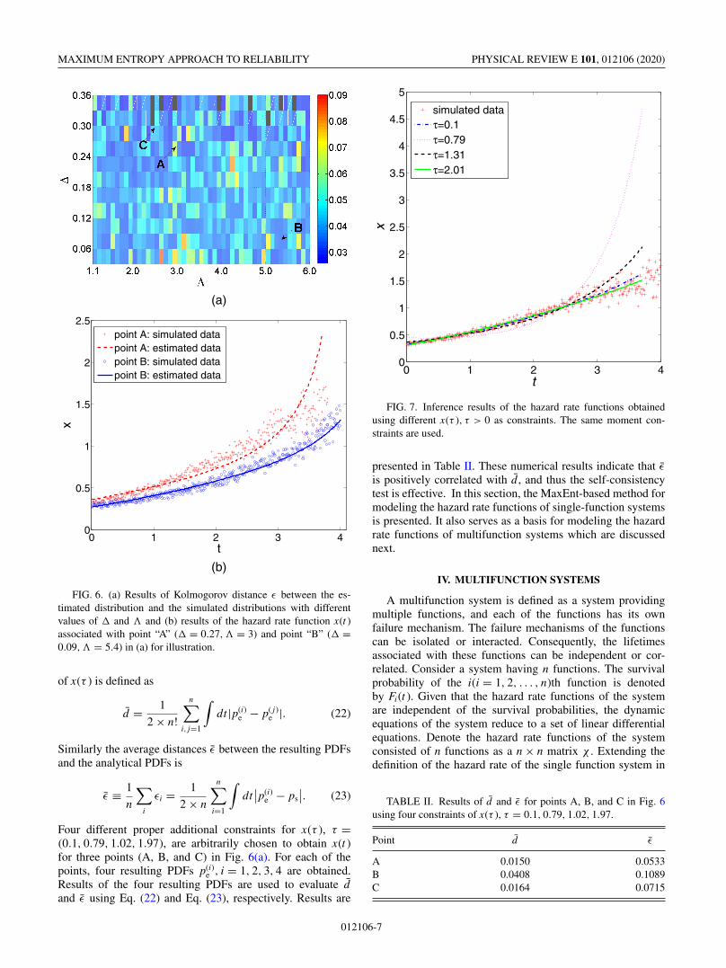
To avoid the conflict between moments and the initial valueof the hazard rate, the hazard rate value at a proper timex(τ ), τ > 0, instead of x(0), can be used. To illustrate theinfluence of the initial value to the estimation result, considerthe region labeled as C in Fig. 6(a), which corresponds toparameters = 0.3 and = 2.4. The hazard rate functionsobtained using four arbitrarily chosen times x(τ ), τ > 0 asconstraints are presented in Fig. 7. It shows that different localinformation can lead to slightly different results.

The second issue relates to the correctness and consistencyof the inference. For any nontrivial hazard rate estimationproblems the true hazard rate is unknown; otherwise, it willnot be a problem at the first place. Therefore, measures areneeded to ensure the results obtained using the developedmethod are reliable. One measure for the evaluation is to com-pare results obtained using different choices of the additionalconstraints. This measure can be made using Kolmogorov dis-tance between two sets of results. The comparison can looselybe seen as a self-consistency test. The average distance dbetween a series of resulting PDFs with additional constraints

012106-6

MAXIMUM ENTROPY APPROACH TO RELIABILITY PHYSICAL REVIEW E 101, 012106 (2020)

0 1 2 3 40

0.5

1

1.5

2

2.5

t

x

ponit A: simulated dataponit A: estimated dataponit B: simulated dataponit B: estimated data

0 1 2 3 40

0.5

1

1.5

2

2.5

t

(b)

(a)

x

point A: simulated datapoint A: estimated datapoint B: simulated datapoint B: estimated data

FIG. 6. (a) Results of Kolmogorov distance ε between the es-timated distribution and the simulated distributions with differentvalues of and and (b) results of the hazard rate function x(t )associated with point “A” ( = 0.27, = 3) and point “B” ( =0.09, = 5.4) in (a) for illustration.

of x(τ ) is defined as

d = 1

2 × n!

n∑i, j=1

∫dt |p(i)

e − p( j)e |. (22)

Similarly the average distances ε between the resulting PDFsand the analytical PDFs is

ε ≡ 1

n

∑i

εi = 1

2 × n

n∑i=1

∫dt

∣∣p(i)e − ps

∣∣. (23)

Four different proper additional constraints for x(τ ), τ =(0.1, 0.79, 1.02, 1.97), are arbitrarily chosen to obtain x(t )for three points (A, B, and C) in Fig. 6(a). For each of thepoints, four resulting PDFs p(i)

e , i = 1, 2, 3, 4 are obtained.Results of the four resulting PDFs are used to evaluate dand ε using Eq. (22) and Eq. (23), respectively. Results are

0 1 2 3 40

0.5

1

1.5

2

2.5

3

3.5

4

4.5

5

tx

simulated dataτ=0.1τ=0.79τ=1.31τ=2.01

FIG. 7. Inference results of the hazard rate functions obtainedusing different x(τ ), τ > 0 as constraints. The same moment con-straints are used.

presented in Table II. These numerical results indicate that ε

is positively correlated with d , and thus the self-consistencytest is effective. In this section, the MaxEnt-based method formodeling the hazard rate functions of single-function systemsis presented. It also serves as a basis for modeling the hazardrate functions of multifunction systems which are discussednext.

IV. MULTIFUNCTION SYSTEMS

A multifunction system is defined as a system providingmultiple functions, and each of the functions has its ownfailure mechanism. The failure mechanisms of the functionscan be isolated or interacted. Consequently, the lifetimesassociated with these functions can be independent or cor-related. Consider a system having n functions. The survivalprobability of the i(i = 1, 2, . . . , n)th function is denotedby Fi(t ). Given that the hazard rate functions of the systemare independent of the survival probabilities, the dynamicequations of the system reduce to a set of linear differentialequations. Denote the hazard rate functions of the systemconsisted of n functions as a n × n matrix χ . Extending thedefinition of the hazard rate of the single function system in

TABLE II. Results of d and ε for points A, B, and C in Fig. 6using four constraints of x(τ ), τ = 0.1, 0.79, 1.02, 1.97.

Point d ε

A 0.0150 0.0533B 0.0408 0.1089C 0.0164 0.0715

012106-7

DU, MA, WEI, GUAN, AND SUN PHYSICAL REVIEW E 101, 012106 (2020)

FIG. 8. Schematic of the reducible and irreducible cases for adouble-function system. The ellipse with the red borderline denotesthe event that the function a works, and the blue ellipse denotesthe event that the function b works. (1) The reducible case wherethe event that the function a works and the event that the functionb works are not strongly correlated. In this case, the intersectionbetween the sets A and B does not affect the reducibility of the matrixχ . (2) The irreducible case where the function b works only if thefunction a also works, i.e., B ⊆ A.

Eq. (1) to a multidimensional case, the dynamic equations ofthe system can be written using a matrix form as

dF

dt= −χF, (24)

where F = (F1, F2, . . . , Fn)T and χ is a n × n hazard ratematrix.

Note that the above equation is obtained based on thecondition that the hazard rate x or χ only depends on timet and is independent of F . For single function systems, thex(t ) and F (t ) are independent variables, because there isno physical interaction or statistical correlation in samplingduring the aging processes. For multifunction systems, itshould be regarded as an approximation for the hazard rate.A sufficient condition for the linear assumption to hold ispresented in Appendix D.

It is worth mentioning that the difference between a single-variable hazard rate x and a multidimensional hazard ratematrix χ is not only the dimension. The term x is only relatedto the probability distribution (if one knows the PDF, thenx can directly be calculated and vice versa); however, theterm χ also encodes the information of the interaction amongdifferent functions in the aging process. Depending on theinteraction, two cases are discussed below.

A. Reducibility of hazard-rate matrices

The nonincreasing nature of the survival probability Fi(t )implies that

dFi

dt� 0, (25)

and dFi/dt and Fi approach zero simultaneously. These twobasic properties will result in a constraint on the hazard ratematrix χ .

To illustrate this consider the following simplest case: adouble-function system shown in Fig. 8. To avoid confusion,the two functions are labeled by a and b. The ellipses Aand B represent the domains that functions a and b work,respectively.

These are two typical cases of the double-function system.The first one shown in Fig. 8(1) denotes the case that a and

TABLE III. Four states of a double-function system in a re-ducible case.

States Function a Function b

1 Work Work2 Work Break down3 Break down Work4 Break down Break down

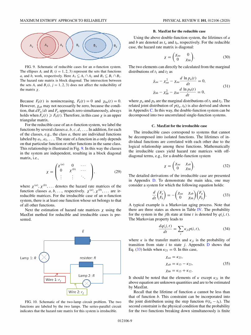
b are not fully correlated. In this case the system has fourstates listed in Table III, labeled by 1,2,3,4. Similarly, thesecond case presented in Fig. 8(2) denotes that if the functionb works, then function a must work, i.e., B ⊆ A. In this casethe system has three states listed in Table IV, labeled by 1,2,3.A typical example for this case is a series-parallel electriccircuit presented in Fig. 10, where the two functions of thesystem are denoted by the two lamps. One can see that if lamp2 works lamp 1 must work and thus this system contains onlythree states. It can be shown that for the first case the hazardmatrix χ must be diagonal or said reducible. For the secondcase χ is an upper triangular matrix or said irreducible.

Consider the first case; without loss of generality the initialstate of the system is assumed to be 2 in Table III. This initialstate corresponds to the following condition:(

Fa(0)Fb(0)

)=

(10

). (26)

Because Fb(t ) is nonincreasing, Fb(t ) = 0. Since dFb/dt andFb approach zero simultaneously, one has

dFb

dt= χbaFa(t ) = 0

and χba(t ) = 0. Similarly, assuming the initial state of thesystem is state 3 in Table III, the initial condition is(

Fa(0)Fb(0)

)=

(01

). (27)

Because Fa(t ) is nonincreasing, Fa(t ) = 0. As dFa/dt and Fa

approach zero simultaneously, one gets

dFa

dt= χabFb(t ) = 0

and χab(t ) = 0. Therefore, in this case χ is diagonal.The second case shown in Fig. 8(2) indicates Fa(t ) � Fb(t ).

Assuming the system is initially at state 2 in Table III, theinitial condition is (

Fa(0)Fb(0)

)=

(10

). (28)

TABLE IV. Three states of a double-function system in an irre-ducible case.

States Function a Function b

1 Work Work2 Work Break down3 Break down Break down

012106-8

MAXIMUM ENTROPY APPROACH TO RELIABILITY PHYSICAL REVIEW E 101, 012106 (2020)

FIG. 9. Schematic of reducible cases for an n-function system.The ellipses Ai and Bi (i = 1, 2, 3) represent the sets that functionsai and bi work, respectively. Here A3 ⊆ A1 ∩ A2 and B3 ⊆ B1 ∩ B2.The hazard rate matrix is block diagonal. The intersection betweenthe sets Ai and Bj (i, j = 1, 2, 3) does not affect the reducibility ofthe matrix χ .

Because Fb(t ) is nonincreasing, Fb(t ) = 0 and χba(t ) = 0.However, χab may not necessarily be zero, because the condi-tion, that dFa/dt and Fa approach zero simultaneously, alwaysholds when Fa(t ) � Fb(t ). Therefore, in this case χ is an uppertriangular matrix.

For the reducible case of an n-function system, we label thefunctions by several classes a, b, c, d, . . .. In addition, for eachof the classes, e.g., the class a, there are individual functionslabeled by a1, a2, . . .. The state of a function in a only dependson that particular function or other functions in the same class.This relationship is illustrated in Fig. 9. In this way the classesin the system are independent, resulting in a block diagonalmatrix, i.e.,

χ =

⎛⎜⎝

χ (a) 0 · · ·0 χ (b) · · ·...

.... . .

⎞⎟⎠, (29)

where χ (a), χ (b), . . . denotes the hazard rate matrices of thefunction classes a, b, . . ., respectively. χ (a), χ (b), . . . are ir-reducible matrices. For the irreducible case of an n-functionsystem, there is at least one function whose set belongs to thatof all other functions.

Next the estimation of hazard rate matrices χ using theMaxEnt method for reducible and irreducible cases is pre-sented.

FIG. 10. Schematic of the two-lamp circuit problem. The twofunctions are labeled by the two lamps. The series-parallel circuitindicates that the hazard rate matrix for this system is irreducible.

B. MaxEnt for the reducible case

Using the above double-function system, the lifetimes of aand b are denoted as ta and tb, respectively. For the reduciblecase, the hazard rate matrix is diagonal:

χ =(

χaa 00 χbb

). (30)

The two elements can directly be calculated from the marginaldistributions of t1 and t2 as

χaa − χ2aa − χaa

d ln pa(t )

dt= 0,

χbb − χ2bb − χbb

d ln pb(t )

dt= 0,

(31)

where pa and pb are the marginal distributions of t1 and t2. Therelated joint distribution of p(ta, tb) is also derived and shownin Appendix C. In this way, the double-function system can bedecomposed into two uncorrelated single-function systems.

C. MaxEnt for the irreducible case

The irreducible cases correspond to systems that cannotbe decomposed into isolated functions. The lifetimes of in-dividual functions are correlated with each other due to thelogical relationship among these functions. Mathematicallythe irreducible cases yield hazard rate matrices with off-diagonal terms, e.g., for a double-function system

χ =(

χaa χab

0 χbb

). (32)

The detailed derivations of the irreducible case are presentedin Appendix D. To demonstrate the main idea, one mayconsider a system for which the following equation holds:

d

dt

(Fa

Fb

)= −

(χaa χab

0 χbb

)(Fa

Fb

). (33)

A typical example is a Markovian aging process. Note thatthere are three states as shown in Table IV. The probabilityfor the system in the jth state at time t is denoted by q( j, t ).The Markovian property leads to

dq( j, t )

dt=

∑i

κ ji p(i, t ), (34)

where κ is the transfer matrix and κ ji is the probability oftransition from state i to state j. Appendix D shows thatEq. (33) holds when κ21 = 0. In this case,

χaa = κ23,

χab = κ13 − κ23,

χbb = κ13 + κ12.

(35)

It should be noted that the elements of κ except κ21 in theabove equation are unknown quantities and are to be estimatedby MaxEnt.

Recall that the lifetime of function a cannot be less thanthat of function b. This constraint can be incorporated intothe joint distribution using the step function θ (ta − tb). Thesecond constraint is the physical condition that the probabilityfor the two functions breaking down simultaneously is finite

012106-9

DU, MA, WEI, GUAN, AND SUN PHYSICAL REVIEW E 101, 012106 (2020)

when κ13 = 0. The condition of κ13 = 0 is the probabilityof transition from the normal state to the failure state. Thisconstraint can be incorporated into the joint distribution usingthe delta function δ(ta − tb). The detailed proof is given inAppendix D. Based on the above constraints, the joint dis-tribution is written

p(ta, tb) = (1 − μ)pN(ta, tb)θ (ta − tb)

+ μpA(ta)δ(ta − tb),(36)

where θ (·) denotes the step function and δ(·) denotes the deltafunction. In the above equation pN and

pA = 1

μκ13 exp

(∫ t

0κ22dt

)(37)

are both normalized PDFs; 0 < μ < 1 is the total probabilitythat the two functions break down simultaneously. pN and pA

can be determined by MaxEnt as

δS = −∫∫

DpN(ta, tb)[ln pN(ta, tb) + αN]dtadtb

−∫∫

DpN(ta, tb)

[∑i

βN,ihN,i(ta, tb)

]dtadtb

−∫

pA(t )

[ln pA(t ) + αA +

∑i′

βA,i′gA,i′ (t )

]dt

= 0, (38)

where D denotes that the domain of ta > tb, αN, βN,i, αA, βA,i′

are the Lagrangian multipliers and pN and pA are independentfunctions.

The connection between the hazard rate matrix and themarginal distributions can then be constructed as the follow-ing equations:

dχaa

dt− χ2

aa

pN,a − pN,b

pN,a− χaa

d ln pN,a

dt= 0,

dχbb

dt− χ2

bb − χbbd ln pb

dt= 0,

χab = μχbbpA

pb− χaa,

(39)

where pN,a and pN,b are the marginal distributions relatedto the PDF of pN(ta, tb) and pb = (1 − μ)pN,b + μpA is themarginal distribution related to the joint PDF of p(ta, tb). Thesolution to the above equation is the resulting hazard ratematrix of the system.

D. Two-lamp circuit model

A two-lamp circuit shown in Fig. 10 is used to represent adouble-function system for demonstration. The two functionsof the system are denoted by the two lamps. One can see thatif lamp 2 works lamp 1 must work. This dependence indicatesthe system is irreducible. The degradation driving factor in theproblem is the heat generation of the two wires.

In the model the physical degradation is also related to thetemperature of the wires. The heat conductance between thewires is also considered in this two-lamp circuit model.

The equation of heat conductance is assumed as

dT1

dt= −ϒT1 + ϒT2,

dT2

dt= −ϒT2 + ϒT1,

(40)

where T1(2) denote the temperature of wire 1(2) and ϒ isassumed as a material dependent constant. For demonstrationpurposes, the regime where the temperatures are much higherthan the Debye temperature is considered. The resistance isproportional to the temperature [41], i.e., r1, r2 ∝ T , and theresistances follow the equation

dr1

dt= −ϒr1 + ϒr2 + �1,

dr2

dt= −ϒr2 + ϒr1 + �2,

(41)

where the first two terms in the right hand side representthe heat conduction between the two wires. The term ϒ isassumed as a material dependent constant, and the term �1(2)

represents the heat generation of the two wires. The heat gen-eration of wire 1(2) is proportional to its power I2

1(2) × r1(2),where I1(2) denote the electric current in wire 1(2). UsingKirchhoff’s law, the electric current in the circuit model canbe directly calculated, and is presented in Appendix E. Theheat generation variables read

�1 = 1r1

((2R + r2)

3R2 + 2(r1 + r2)R + r1r2

)2

,

�2 = 2r2

(R

3R2 + 2(r1 + r2)R + r1r2

)2

,

(42)

where R is the overall resistance of the lamps and the resistor.1(2) is the effective ratio parameter. For illustration purposes,let 21 = 2 ≡ .

The terms pN,1, pN,2, and pA can be estimated separately.Note that in this case Eq. (36) indicates that pN,1(0) = 0. Thisprior knowledge leads to the breaking down of the problem.To avoid that a nonlinear measure of the integral of t , i.e.,dt → t dt , is added. This modification of the measure isequivalent to the maximization of the cross entropy. The proofis as follows:∫

(−p ln p)ν(t )dt ≡ −∫

pν(t ) lnpν(t )

ν(t )dt, (43)

where ν(t ) is the proper measure. Recall the constraint of∫pν dt = 1. The variational term of the entropy is

δ

[∫(−p ln p)ν dt − α

∫pν dt

]

= δ

[−

∫pν ln

pν

νdt − α

∫pν dt

]

= δ

[−

∫pν ln

pν

exp(−αν )νdt − αp

∫pν dt

]

= δ

[−

∫p ln

p

p0dt − αp

∫p dt

], (44)

012106-10

MAXIMUM ENTROPY APPROACH TO RELIABILITY PHYSICAL REVIEW E 101, 012106 (2020)

where α = αp + αν and αp are Lagrange multipliers,p0 ≡ exp(−αν )ν(t ) is a prior distribution which satisfiesexp(−αν )

∫ν(t )dt = 1, and p ≡ pν is the variational PDF.

Note that this modification requires prior knowledge abouthazard rates of the two functions and its time derivations neart = 0.

To demonstrate the effectiveness of the method, numericalexperiments are made to simulate actual experimental data.Parameters of R = 1, ϒ = 0.01, and ( = 0.09, = 2) areused to generate simulated data. In this setting the numericalcalculation yields μ ≈ 0.1266. In estimation χ (τ = 0.32) isused as the additional constraint. The estimated results areshown in Fig. 11, which are close to the simulated data.These results indicate that the method combining the linearassumption with the double-moment constraint is effective toanalyze a multifunction system.

V. CONCLUSIONS AND DISCUSSIONS

Inspired by statistical mechanics in physics, as a theoryof statistical inference, a MaxEnt approach to reliability isdeveloped in this study, allowing for constructing the hazardrate function in a rational manner. The hazard rate functionis a fundamental quantity in the disciplines of reliability andrisk analysis, characterizing the aging process of a system. Inparticular, the time-dependent hazard rate can fully describethe dynamics of the aging system. The basic idea of thedeveloped method is to recast an estimation problem to aprobabilistic inference problem using the principle of max-imum entropy. The most probable hazard rate function is theone that maximizes the information entropy. Information suchas observed data in terms of statistical moments are used asconstraints to obtain the most probable hazard rate function.

It is shown that different shapes of hazard rate functions,such as the widely observed bathtub shape in engineering,upside down bathtub shape in biological system, and W/Nshapes can all be interpreted as the most probable hazard rateunder certain constraints. In addition to the single-functionsystem, the multifunction system consisting of multiple in-dividual isolated and/or correlated functions is investigatedby extending the hazard rate function to a multidimensionalhazard rate matrix. For a system with isolated functions, it canbe reduced to a set of independent hazard rate functions andyield a block diagonal hazard rate matrix. For a system withcorrelated functions, the interaction terms yield off-diagonalterms in the hazard rate matrix and the system is the so-calledirreducible system. The overall method is demonstrated usingnumerical examples, and the effectiveness of the method isverified for both single- and multifunction systems.

The application of the proposed methods in general in-volves the following steps. (1) Process the observed lifetimedata as testable information, e.g., calculate the statistical mo-ments; (2) choose several time points τ1, τ2, . . . and evaluatethe corresponding hazard rate x(τ1), x(τ2), . . . from the life-time data; (3) use the hazard rate at one chosen time point andobtain the parameters, i.e., the Lagrange multipliers, using thetestable information as constraints; (4) perform consistencycheck following step (3) using other time points.

To understand the “physical” meaning of parameters, theinformation beyond lifetime is necessary. In this paper, the

0 2 4 6 80

0.1

0.2

0.3

0.4

0.5

0.6

0.7

t

χ 11

simulated dataestimated data

(a)

0 2 4 6 8

−0.4

−0.2

0

0.2

0.4

0.6

t

χ 12

simulated dataestimated data

(b)

0 2 4 6 80

0.1

0.2

0.3

0.4

0.5

0.6

0.7

0.8

t

χ 22

simulated data

estimated data

(c)

FIG. 11. Comparisons of the estimated components of the hazardrate matrix with the simulated data.

approach is independent of specific systems. This is based onthe assumption that no other information is accessed exceptto the information of lifetime. In realistic applications, thesystem may contain other information, e.g., lifetime data oncomponents, structures, and their correlations and so on. Theinformation can result in different hazard rate functions whenit is used as constraints. Moreover, the linear approximation isapplied in the multifunction cases. The linear approximationmay not be valid and the justification must be carefully made.

012106-11

DU, MA, WEI, GUAN, AND SUN PHYSICAL REVIEW E 101, 012106 (2020)

The features of structures and correlations are also relatedto nonlinearity of multicomponent systems. How to fuse thehierarchical information using the proposed method should tobe further investigated.

In addition, Eq. (7) generates the PDFs belonging tothe exponential family. For specific cases, to generate PDFswhich do not belong to the exponential family, differentequations of motion should be considered. There are atleast two ways to achieve this. One is to adopt a nonlinearmeasure in the integrals, which has been discussed in theprevious section. Another is to construct a distribution F (t ) =exp(−X )φ(X ) where φ(X ) is a suitable function satisfyingdF/dt � 0, φ(0) = 1, such as F (t ) = exp(−X )(1 + X ).

The significance of the developed method lies in the factthat (1) it provides a rational instrument to construct thehazard rate function consistently given any available infor-mation from experimental data, (2) it provides a statisticalmechanics-based approach to interpreting the generation ofdifferent shapes of the hazard rate curves observed in the fieldof reliability over the past few decades, and (3) it providesa theoretical bridge linking the reliability engineering to oneof the most fundamental principles, MaxEnt, in physics. Thisstudy lays out a possible pathway to the enlightened goal inRef. [36], which is “the reliability theory is a new science.”

ACKNOWLEDGMENTS

The work in this study was supported by NationalBasic Program of China (Grant No. 2016YFA0301201),NSFC (Grants No. 11534002 and No. 51975546), NSAF(Grants No. U1730449, No. U1530401, No. U1930402, andNo. U1930403), and Science Challenge Project (Grant No.TZ2018007). The support is greatly acknowledged. The au-thors would like to thank the anonymous reviewers for theirconstructive comments.

APPENDIX A: MOST PROBABILITY DISTRIBUTION ANDTHE EQUATION OF MOTION OF THE HAZARD

RATE FUNCTION

In general, the entropy is given as

S = −∫ tmax

tmin

p(t ) ln p(t )dt, (A1)

where tmin and tmax are the minimum and the maximumlifetime, respectively. We maximize the entropy with momentconstraints using variations

δS = δ

{−

∫ tmax

tmin

dt ′ p(t ′) ln p(t ′) − βi

∫ tmax

tmin

dt ′gi(t′)p(t ′)

−α

∫ tmax

0dt ′(t ′)p(t ′)

}= 0, (A2)

where ∫ tmax

tmin

dt ′gi(t′)p(t ′), (A3)

with i = 1, 2, . . ., are the moments from observation.

The most probable distribution is

p(t ) ={

1Z exp

[ − ∑i βigi(t )

], tmin � t � tmax,

0, else,(A4)

where

Z =∫ tmax

tmin

exp

[−

∑i

βigi(t )

]dt (A5)

is the partition function or so-called normalizing constant inprobability.

The motion equation in Eq. (7) can be also derived fromthe most probable distribution. We use

p(t ) = x exp(−X ), (A6)

where

X (t ) =∫ t

tmin

x(t ′)dt ′, (A7)

to obtain

x(t ) exp[−X (t )] = 1

Zexp

[−

∑i

βigi(t )

]. (A8)

Its derivation with respect to time t reads

x exp(−X ) − x2 exp(−X )

= 1

Zexp

[−

∑i

βigi(t )

][−

∑i

βigi(t )

]. (A9)

Namely,

x − x2 +∑

i

βigi(t )x = 0 (A10)

is obtained. By assuming tmin = 0 and gi(t ) satisfy gi(0) = 0,the initial condition is given by x(0) = 1/Z . Finally, thesolution to Eq. (7) is

x(t ) = x0 exp( − ∑

i βigi)

1 − x0∫ t

0 exp( − ∑

i βigi)dt ′ . (A11)

We define a new function x = x exp[∑

i βigi(t )] and substi-tute it into Eq. (7) to have

˙x = exp

[−

∑i

βigi(t )

]x2. (A12)

Solving Eq. (A12) we obtain

1

x0− 1

xt=

∫ t

0exp

[−

∑i

βigi(t′)

]dt ′. (A13)

The initial condition is x(0) = exp[−∑i βigi(0)]x0 = x0.

From the above equation and x = x exp[−∑i βigi(t )], one

can verify Eq. (A11).

APPENDIX B: NUMBER OF INFLECTION POINTS

The most probable hazard rate function constructed usinga double-moment constraint can have at most one point ofinflection. The proof is given below.

012106-12

MAXIMUM ENTROPY APPROACH TO RELIABILITY PHYSICAL REVIEW E 101, 012106 (2020)

Rewrite Eq. (14) as

x = x(x − β1 − 2β2t ), (B1)

where () denotes d ()/dt . For x > 0 the points of inflec-tion must be located at x = β1 + 2β2t . For convenience wedefine a function y(t ) = β1 + 2β2t . Consider the functionx(t ) − y(t ), where x(t ) is the hazard rate function whichsatisfies Eq. (14). The time derivative of x(t ) − y(t ) is

x − y = x(x − y) − 2β2, (B2)

where the hazard rate function satisfies x(t ) > 0.For β2 < 0, if x(t0) − y(t0) � 0 with t0 > 0 then the above

equation implies that x(t ) − y(t ) > 0 with arbitrary t > t0,i.e., the region x(t ) � y(t ) is the absorption domain forEq. (14) with β2 < 0. Therefore, there is at most one point ofinflection for β2 < 0. More precisely, for β2 < 0, x0 > 0 > β1

and for β2 < 0, x0 � β1 > 0, there is no point of inflection.For β2 < 0, 0 < x0 < β1 there is one point of inflection andthe function is in bathtub shapes.

Similarly, for β2 > 0, if x(t0) − y(t0) � 0 with t0 > 0 thenthe above equation implies that x(t ) − y(t ) < 0 with arbi-trary t > t0, i.e., the region x(t ) � y(t ) is the absorptiondomain for Eq. (14) with β2 > 0. Therefore, there is alsoat most one point of inflection for β2 > 0. More precisely,for β2 > 0, 0 < x0 � β1 and for β2 > 0, x0

∫ ∞0 exp(−β1t −

β2t2)dt > 1, there are no points of inflection; for β2 > 0,

x0∫ ∞

0 exp(−β1t − β2t2)dt = 1 there is one point of inflectionand the function is in upside down bathtub shapes.

The hazard rate for β2 > 0, x0 � β1 is monotonically de-creasing; however, this condition violates Eq. (17). From theabove discussion, the shapes of x(t ) can be divided into threetypes, i.e., the monotonically increasing, the bathtub shape,and the upside down bathtub shape.

It can be shown, as follows, that the hazard rate func-tion constructed using an n-moment constraint contains atmost n − 1 inflection points. For convenience, let y(t ) =∑

n=1 nβntn−1 and the time derivative of x(t ) − y(t ) reads

x − y = x(x − y) −∑n=2

n(n − 1)βntn−2. (B3)

The location of the absorption domain depends on the sign ofy = ∑

n=2 n(n − 1)βntn−2. The function y(t ) here has at mostn − 2 inflection points, i.e., the function y has at most n − 2zero points.

We denote t1, t2, . . . , tn−2 as the zero points and 0 <

t1 < t2 < · · · < tn−2. The sign of y in the time intervals(ti, ti+1), i = 1, 2, . . . , n − 3 and intervals [0, 1), (tn−2,∞) re-mains unchanged. In any one of these time intervals, x(t ) hasat most one inflection point, and therefore x(t ) has a totalof n − 1 inflection points at most. In addition, the n-momentconstraint is capable of generating 2n − 1 types of shapes. Themonotonically decreasing curve has been excluded because itviolates the normalization condition.

APPENDIX C: JOINT AND THE MARGINALDISTRIBUTIONS FOR REDUCIBLE AND IRREDUCIBLE

CASES IN A DOUBLE-FUNCTION SYSTEM

In the reducible cases, the marginal distributions related tothe joint PDF of p(t1, t2) can be obtained by MaxEnt,

S = −∫ ta,max

ta,min

∫ tb,max

tb,min

p(t1, t2)[ln p(t1, t2) − α]dt1dt2

−∑

i

βi

∫ ta,max

ta,min

∫ tb,max

tb,min

hi(t1, t2)p(t1, t2)dt1dt2, (C1)

where α and βi, i = 1, 2, . . . are the Lagrangian multipliersand hi(t1, t2) are the correlation functions. We maximize S toobtain the joint PDF for ti ∈ [ti,min, ti,max], i = a, b as

p(ta, tb) = 1

Zexp

[−

∑i

βihi(ta, tb)

], (C2)

where Z =∫ ta,max

ta,min

∫ tb,max

tb,min

p(ta, tb)dtadtb is the partition func-

tion. The marginal distributions are given as

pa(t ) =∫ tb,max

tb,min

p(t, tb)dtb,

pb(t ) =∫ ta,max

ta,min

p(ta, t )dta. (C3)

In the irreducible cases, we maximize the entropy inEq. (38) and obtain

pN(ta, tb) = 1

ZNexp

[−

∑i

βN,ihN,i(ta, tb)

],

pA(t ) = 1

ZAexp

[−

∑i

βA,igN,i(t )

].

(C4)

The marginal distributions pi(t ) = pN,i(t ) + pA,i(t ), i = a, bare given as

pN,a(t ) = (1 − μ)∫ tb,max

tb,min

dtb pN(t, tb),

pN,b(t ) = (1 − μ)∫ ta,max

ta,min

dta pN(ta, t ),

pA,a(t ) = pA,b(t ) = μpA(t ),

(C5)

where μ is defined as before.

APPENDIX D: MARKOVIAN AGING PROCESS

We consider a Markovin process, and denote the probabil-ity of the trajectory (i1, t1; i2, t2; . . .) as q(i1, t1; i2, t2; . . .). TheMarkovian approximation is

q( jm+1, tm+1| jm, tm; jm−1, tm−1; . . . ; j0, t0)

= q( jm+1, tm+1| jm, tm), (D1)

where the conditional probability q(A|B) denotes the probabil-ity of event A conditional on event B. The diffusion equation

012106-13

DU, MA, WEI, GUAN, AND SUN PHYSICAL REVIEW E 101, 012106 (2020)

isdq( j, t )

dt= lim

t→0

1

t

∑i

[q( j, t |i, t − t ) − δi, j]q(i, t − t ) =∑

i

κ ji p(i, t ). (D2)

The joint PDF p(ta, tb) is related to the trajectory probability. In the irreducible cases, one has

p(ta, tb)t2 = q(3, ta; 2, ta − t ; 2, ta − 2t ; . . . ; 2, tb; 1, tb − t ; 1, tb − 2t ; . . . ; 1, 0), (D3)

where q(3, ta; 2, ta − t ; . . .) is the probability of the trajectory. It is shown that

p(t, t )t2 = q(3, ta; 1, ta − t ; 1, ta − 2t ; . . . ; 1, tb; 1, tb − t ; 1, tb − 2t ; . . . ; 1, 0)

= q(3, ta|1, ta − t )q(1, ta − t ; 1, ta − 2t ; . . . ; 1, tb; 1, tb − t ; 1, tb − 2t ; . . . ; 1, 0)

= q(3, ta|1, ta − t )q(1, ta − t |1, ta − 2t ) . . . q(1,t |1, 0)

= κ13(1 + κ22t )t/tt . (D4)

Furthermore,

p(t, t − t ) = q(3, ta; 2, ta − t ; 1, ta − 2t ; . . . ; 1, tb; 1, tb − t ; 1, tb − 2t ; . . . ; 1, 0)1

t2

= q(3, ta|2, ta − t )q(2, ta − t ; 1, ta − 2t ; . . . ; 1, tb; 1, tb − t ; 1, tb − 2t ; . . . ; 1, 0)1

t2

= q(3, ta|2, ta − t )q(2, ta − t |1, ta − 2t ) . . . q(1,t |1, 0)1

t2

= κ23κ12(1 + κ22t )t/t−1t2 1

t2

= κ23κ12(1 + κ22t )t/t−1. (D5)

The above two equations imply that

p(t, t ) = limt→0

κ13

texp

(∫ t

0κ22dt ′

)= lim

t ′→tδ(t − t ′)κ13 exp

(∫ t

0κ22dt ′′

). (D6)

Comparing the above equation to Eq. (36), one has

μpA = κ13 exp

(∫ t

0κ22dt ′

). (D7)

We rewrite the diffusion equation as

d

dtq1 = I (2→1) − I (1→3) + I (3→1) − I (1→2),

d

dtq2 = −I (2→1) + I (1→2) + I (3→2) − I (2→3),

d

dtq3 = I (2→3) − I (3→2) − I (3→1) + I (1→3),

(D8)

where I (i→ j)(t ) = κ ji p(i, t ) is the current of probability fromi to j at time t .

The survival functions of a and b are denoted as Fa and Fb,respectively. We denote the probability that the system is instate i, i = 1, 2 without previously being in state 3 as Gi. Sucha condition leads to Fa = G1 + G2, and G1, G2, Fb satisfy thefollowing equations:

d

dtG1 = −G1

q1[I (1→2) + I (1→3)] + G2

q2I (2→1),

d

dtG2 = −G2

q2[I (2→1) + I (2→3)] + G1

q1I (1→2),

d

dtFb = −Fb

q2[I (1→2) + I (1→3)]. (D9)

We rewrite the above equation as

d

dt

⎛⎝G1

G2

Fb

⎞⎠ =

⎛⎝−κ12 − κ13 κ21 0

κ12 −κ21 − κ23 00 0 −κ12 − κ13

⎞⎠

⎛⎝G1

G2

Fb

⎞⎠.

(D10)If κ21 = 0, the above equation is reduced to

d

dt

(Fa

Fb

)=

(−κ23 κ23 − κ13

0 −κ13 − κ12

)(Fa

Fb

). (D11)

The hazard rate matrix is

χ = −(−κ23 κ23 − κ13

0 −κ13 − κ12

), (D12)

where the elements of the matrix are to be determined byMaxEnt.

The result of Eq. (39) is obtained as follows. Consid-ering the initial condition Fa(0) = 1, Fb(0) = 1, we rewriteEq. (D11) in integral form as

Fa = exp(−χaa)

[1 −

∫ t

0χab exp(χaa − χbb)dt ′

],

Fb = exp(−χbb).

(D13)

012106-14

MAXIMUM ENTROPY APPROACH TO RELIABILITY PHYSICAL REVIEW E 101, 012106 (2020)

With Fi = ∫ t0 pi(t ′)dt ′, i = a, b, we take the time derivative of

the above equation to have

pa = χaa exp(−χaa)

[1 −

∫ t

0χab exp(χaa − χbb)dt ′

]

+ χab exp(−χbb),

pb = χbb exp(−χbb), (D14)

where pa = pN,a(t ) + pA,a(t ) and pb = pN,b(t ) + pA,b(t ) arethe marginal distributions shown in Eq. (C5). Combining theabove equations with Eq. (D7) and taking the time derivativeagain, one can verify Eq. (39). Given ta,min = tb,min = 0 andta,max = tb,max = tmax, the solution to Eq. (39) is finally ob-tained as

χaa = − pN,a∫ t0 dt ′(pN,a − pN,b)

,

χbb = pb

1 − ∫ t0 dt ′ pb

,

χab = μpA

1 − ∫ t0 dt ′ pb

+ pN,a∫ t0 dt ′(pN,a − pN,b)

. (D15)

APPENDIX E: POWER OF THE WIRES IN THETWO-LAMP CIRCUIT MODEL

Let P1(2) denote the power of wire 1(2). The term E denotesthe electromotive force of the source. The currents in wires 1and 2 are

I1 = E/

[R+r1+R(R + r2)

2R + r2

]= E (2R + r2)

3R2 + 2(r1 + r2)R + r1r2,

I2 = I1R

2R + r2= ER

3R2 + 2(r1 + r2)R + r1r2. (E1)

Consequently,

P1 = I21 r1 ∝

(2R + r2

3R2 + 2(r1 + r2)R + r1r2

)2

r1,

P2 = I22 r2 ∝

(R

3R2 + 2(r1 + r2)R + r1r2

)2

r2. (E2)

We introducing an effective coefficient term to the aboveequation to obtain Eq. (42).

0 10 20 30 40 50 600

0.01

0.02

0.03

0.04

0.05

0.06

Time(days)

Dea

th r

ate

FIG. 12. Estimated death rate curve for fruit fly.

APPENDIX F: BIOLOGICAL EXAMPLE: FRUIT FLY

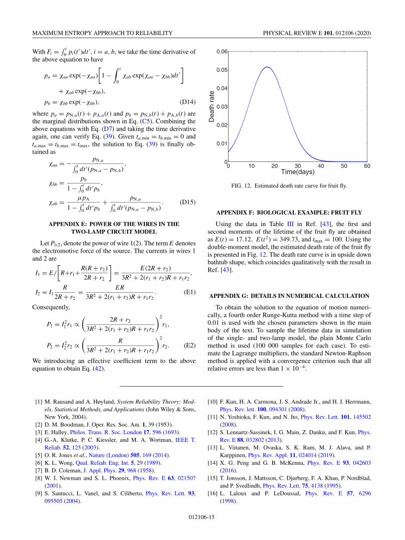
Using the data in Table III in Ref. [43], the first andsecond moments of the lifetime of the fruit fly are obtainedas E (t ) = 17.12, E (t2) = 349.73, and tmax = 100. Using thedouble-moment model, the estimated death rate of the fruit flyis presented in Fig. 12. The death rate curve is in upside downbathtub shape, which coincides qualitatively with the result inRef. [43].

APPENDIX G: DETAILS IN NUMERICAL CALCULATION

To obtain the solution to the equation of motion numeri-cally, a fourth order Runge-Kutta method with a time step of0.01 is used with the chosen parameters shown in the mainbody of the text. To sample the lifetime data in simulationof the single- and two-lamp model, the plain Monte Carlomethod is used (100 000 samples for each case). To esti-mate the Lagrange multipliers, the standard Newton-Raphsonmethod is applied with a convergence criterion such that allrelative errors are less than 1 × 10−4.

[1] M. Rausand and A. Høyland, System Reliability Theory: Mod-els, Statistical Methods, and Applications (John Wiley & Sons,New York, 2004).

[2] D. M. Boodman, J. Oper. Res. Soc. Am. 1, 39 (1953).[3] E. Halley, Philos. Trans. R. Soc. London 17, 596 (1693).[4] G.-A. Klutke, P. C. Kiessler, and M. A. Wortman, IEEE T.

Reliab. 52, 125 (2003).[5] O. R. Jones et al., Nature (London) 505, 169 (2014).[6] K. L. Wong, Qual. Reliab. Eng. Int. 5, 29 (1989).[7] B. D. Coleman, J. Appl. Phys. 29, 968 (1958).[8] W. I. Newman and S. L. Phoenix, Phys. Rev. E 63, 021507

(2001).[9] S. Santucci, L. Vanel, and S. Ciliberto, Phys. Rev. Lett. 93,

095505 (2004).

[10] F. Kun, H. A. Carmona, J. S. Andrade Jr., and H. J. Herrmann,Phys. Rev. lett. 100, 094301 (2008).

[11] N. Yoshioka, F. Kun, and N. Ito, Phys. Rev. Lett. 101, 145502(2008).

[12] S. Lennartz-Sassinek, I. G. Main, Z. Danku, and F. Kun, Phys.Rev. E 88, 032802 (2013).

[13] L. Viitanen, M. Ovaska, S. K. Ram, M. J. Alava, and P.Karppinen, Phys. Rev. Appl. 11, 024014 (2019).

[14] X. G. Peng and G. B. McKenna, Phys. Rev. E 93, 042603(2016).

[15] T. Jonsson, J. Mattsson, C. Djurberg, F. A. Khan, P. Nordblad,and P. Svedlindh, Phys. Rev. Lett. 75, 4138 (1995).

[16] L. Laloux and P. LeDoussal, Phys. Rev. E 57, 6296(1998).

012106-15

DU, MA, WEI, GUAN, AND SUN PHYSICAL REVIEW E 101, 012106 (2020)

[17] A. Dechant, E. Lutz, D. A. Kessler, and E. Barkai, Phys. Rev. X4, 011022 (2014).

[18] P. Lunkenheimer, R. Wehn, U. Schneider, and A. Loidl, Phys.Rev. Lett. 95, 055702 (2005).

[19] S. Boettcher, D. M. Robe, and P. Sibani, Phys. Rev. E 98,020602(R) (2018).

[20] Y. T. Lou, J. F. Xia, W. Tang, and Y. Chen, Phys. Rev. E 96,062418 (2017).

[21] H. Pham and C. D. Lai, IEEE T. Reliab. 56, 454 (2007).[22] D. V. Lindley, J. R. Stat. Soc.: Ser. B 20, 102 (1958).[23] Z. Ahmad, G. G. Hamedani, and N. S. Butt, Pak. J. Stat. Oper.

Res. 15, 87 (2019).[24] C. D. Lai, M. Xie, and D. N. P. Murthy, Handbook Stat. 20, 69

(2001).[25] R. Jiang, Reliab. Eng. Syst. Safe. 119, 44 (2013).[26] R. Jiang, Int. J. Perform. Eng. 9, 569 (2013).[27] N. Ebrahimi, Sankhya Ser. A 58, 48 (1996).[28] N. Ebrahimi, Sankhya Ser. A 62, 236 (2000).[29] M. Asadi and N. Ebrahimi, Stat. Probab. Lett. 49, 263 (2000).[30] M. Asadi, N. Ebrahimi, G. G. Hamedani, and E. S. Soofi,

J. Appl. Prob. 41, 379 (2004).

[31] M. Asadi, N. Ebrahimi, E. S. Soofi, and S. Zarezadeh, Nav. Res.Log. 61, 427 (2015).

[32] A. D. Crescenzo and M. Longobard, J. Appl. Prob. 39, 434(2002).

[33] X. Guan, R. Jha, and Y. Liu, J. Intell. Manufact. 23, 163(2012).

[34] X. Guan, R. Jha, and Y. Liu, Probab. Eng. Mech. 29, 157(2012).

[35] P. Rocchi and G. Capacci, Entropy 17, 502 (2015).[36] P. Rocchi, Reliability is a New Science (Springer International

Publishing, Berlin, 2017).[37] C. E. Shannon, Bell Syst. Tech. J. 27, 379 (1948).[38] E. T. Jaynes, Phys. Rev. 106, 620 (1956).[39] E. T. Jaynes, Phys. Rev. 108, 171 (1957).[40] E. T. Jaynes, Proc. IEEE 70, 939 (1982).[41] See, for example, N. W. Ashcroft and N. David Mermin, Solid

State Physics (Saunders College, Philadelphia, 1976), Chap. 26.[42] See, for example, C. A. Fuchs and J. V. D. Graaf, IEEE Trans.

Inf. Theory 45, 1216 (1999).[43] J. R. Carey, P. Liedo, and J. W. Vaupel, Experiment. Gerontol.

30, 605 (1995).

012106-16