Maximin Utility with Renewable and Nonrenewable Resources

Jon M. Conrad

In the spirit of Rawls (1971):

• If you did not know the generation into which you would be born, what rules would you want society to adopt relating to consumption, the rate of harvest from a renewable resource, and the rate of extraction from a nonrenewable resource?

• You might want rates of consumption harvest, and extraction which maximized the utility of the least-well-off generation. This is known as the maximin criterion.

• In this paper, Conrad numerically explores the maximin criterion in a discrete-time model with a renewable and a nonrenewable resource and a finite number of non-overlapping generations.

The Rawlsian social contract

Takes the form of a vector of four rates:

• α: the fraction of a manufactured good that is consumed• β : the fraction of a renewable resource that is harvested• γF : the fraction of a nonrenewable resource extracted for

production of the manufactured good, and • γU : the fraction of the nonrenewable resource extracted

for direct consumption (utility).

These rates are adopted by all generations.

The maximin social contract

• The maximin social contract does not lead to equal utility across a finite number of generations

• But it typically results in an equitable intergenerational distribution of utility, as measured by the Gini coefficient.

• We explore how the four rates in the maximin social contract depend on initial conditions and the number of generations.

Introduction Rawls (1971) asked what social contract one would want in place if

• "no one knows his place in society, his class position or social status, nor does anyone know his fortune in the distribution of natural assets and abilities, his intelligence, strength, and the like. … The principles of justice are chosen behind a veil of ignorance." (Rawls, 1971, p.11.)

• To Rawls, the rational individual, not knowing his or her lot in life, would want rules in place that would maximize the utility of the least-well-off individual.

• This is now referred to as the maximin criterion.

II. The Model (a)

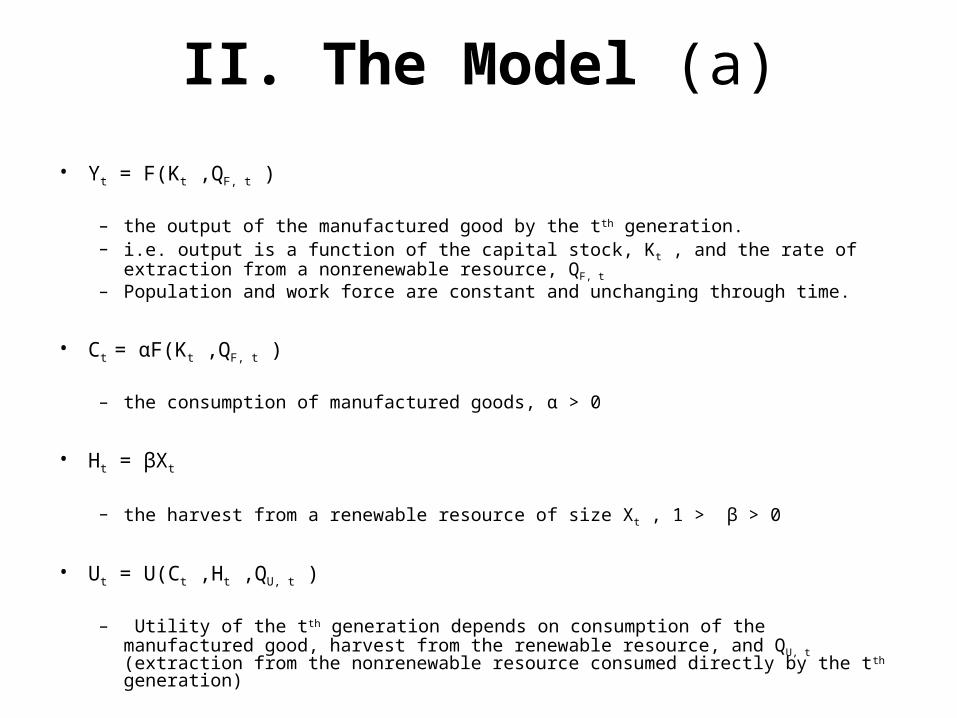
• Yt = F(Kt ,QF, t )

– the output of the manufactured good by the tth generation.– i.e. output is a function of the capital stock, Kt , and the rate of extraction from a

nonrenewable resource, QF, t – Population and work force are constant and unchanging through time.

• Ct = αF(Kt ,QF, t )

– the consumption of manufactured goods, α > 0

• Ht = βXt

– the harvest from a renewable resource of size Xt , 1 > β > 0

• Ut = U(Ct ,Ht ,QU, t )

– Utility of the tth generation depends on consumption of the manufactured good, harvest from the renewable resource, and QU, t (extraction from the nonrenewable resource consumed directly by the tth generation)

• QF, t = γFRt and QU, t = γURt

• denote the levels of extraction for production of the manufactured good and for direct consumption when the remaining reserves of the nonrenewable resource are Rt

• 1 > γF > 0 , 1 > γU > 0 , 1 > (γF + γU ) > 0 ,

• Rt+1 = [1 - (γF + γU)] Rt

• the dynamics of remaining reserves,

• Kt+1 = Kt + (1- α)F(Kt ,QF, t )

• the dynamics of the capital stock,

• Xt+1 = [1- β + r(1- Xt/Xc )]Xt

• the dynamics of the renewable resource• r > 0 is the intrinsic growth rate• Xc > 0 is the environmental carrying capacity• and it is assumed that |1- r + β | < 1 (to avoid chaos)

• Let t = 0,1,2,...,T be the number of generations under consideration, where t = 0 is the current generation and T is the terminal generation

• [α, β, γF , γU] denotes a social contract, invariant across the generations.

The optimization problem

Seeks to find the social contract which will

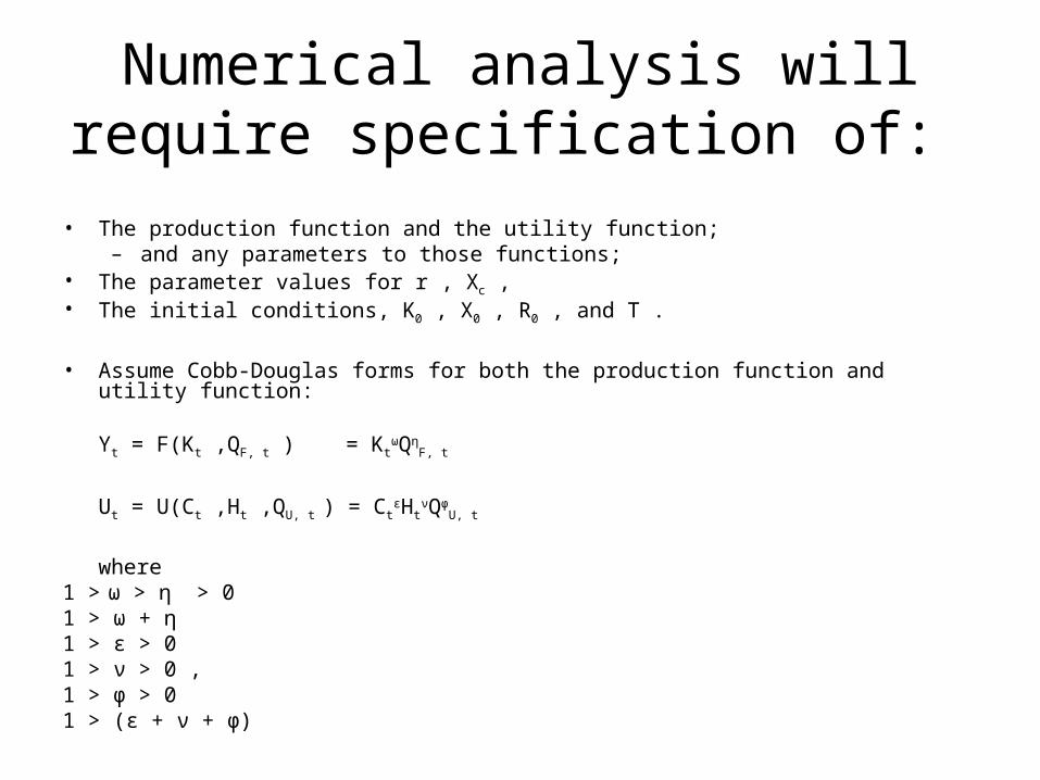
Numerical analysis will require specification of:

• The production function and the utility function;– and any parameters to those functions;

• The parameter values for r , Xc , • The initial conditions, K0 , X0 , R0 , and T .

• Assume Cobb-Douglas forms for both the production function and utility function:

Yt = F(Kt ,QF, t ) = KtωQη

F, t

Ut = U(Ct ,Ht ,QU, t ) = CtεHt

νQφU, t

where1 > ω > η > 0 1 > ω + η 1 > ε > 0 1 > ν > 0 ,1 > φ > 0 1 > (ε + ν + φ)

Properties

• The production function and the utility function exhibit declining marginal product or utility, respectively, and both functions are homogeneous of degree less than one.

• These functions both have unitary elasticity of substitution between inputs (in the case of the production function) or commodities (in the case of the utility function).

• This will allow capital to substitute for extraction of the nonrenewable resource in production

• And for consumption or harvest to substitute for extraction from the nonrenewable resource in utility.

• In the social contract, [α, β, γF , γU], a positive, steady-state, level for Xt will be achieved at

X* = Xc (r - β)/r

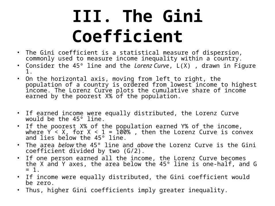
III. The Gini Coefficient • The Gini coefficient is a statistical measure of dispersion, commonly used to

measure income inequality within a country. • Consider the 45º line and the Lorenz Curve, L(X) , drawn in Figure 1. • On the horizontal axis, moving from left to right, the population of a country

is ordered from lowest income to highest income. The Lorenz Curve plots the cumulative share of income earned by the poorest X% of the population.

• If earned income were equally distributed, the Lorenz Curve would be the 45º line.

• If the poorest X% of the population earned Y% of the income, where Y < X, for X < 1 = 100% , then the Lorenz Curve is convex and lies below the 45º line.

• The area below the 45º line and above the Lorenz Curve is the Gini coefficient divided by two (G/2).

• If one person earned all the income, the Lorenz Curve becomes the X and Y axes, the area below the 45º line is one-half, and G = 1.

• If income were equally distributed, the Gini coefficient would be zero. • Thus, higher Gini coefficients imply greater inequality.

More on Gini

IV. Maximin Social Contracts

• To start, we consider a simple maximin problem where T = 10 , implying that 11 generations will be bound by the social contact [α, β, γF , γU].

• Table 1 shows an initial spreadsheet where the social contract has been arbitrarily set to [α, β, γF , γU] = [0.90, 0.20, 0.05, 0.05] , as indicated by the values in cells I8:I11

• Other parameter values are shown in cells B3:B13.

Simulation 1

• Given these parameter values, initial conditions, and the social contract, the spreadsheet in Table 1 simulates the values for consumption, harvest from the renewable resource, extraction for utility, extraction for production, the capital stock, remaining reserves, and utility in columns B through I.

• Column J indicates the rank of each utility level and column K computes the term (T + 2 - RankUt )Ut , whose sum will be used in computing the Gini coefficient.

• In cells I28:I30 we use the Excel functions =MIN($I$16:$I$26) to return the minimum utility, =MAX($I$16:$I$26) to return the maximum utility (just for comparison to the minimum), and compute the Gini coefficient for the utility vector using Equation (2).

• For this initial social contract we see utility monotonically declines from U0 = 3.28787 to U10 = 2.86017 .

• The Gini coefficient registers G = 0.02357 .

• In this initial spreadsheet, the steady-state stock for the renewable resource is X* = 80 , which is reached in t = 1.

Simulation 1 (Optimised)

• We now use Excel’s Solver to maximize the minimum utility in cell I28 by changing the social contract in cells I8:I11.

• The maximin social contract and time paths for consumption, harvest, extraction, the capital stock, remaining reserves, and utility are given in Table 2. For this numerical example the maximin social contract is given by [α, β, γF , γU] = 0.634, 0.5, 0.082, 0.087] . The maximized minimum utility is U2= 3.87149 .

• Perhaps surprisingly, we see that the maximin social contract is Pareto superior to the initial social contact in that all utility levels have been increased.

• When the initial stock of the renewable resource exceeds the stock necessary to support maximum sustainable yield, XMSY , the maximin social contract will choose β so that X* = XMSY = Xc/2 . But, as noted above, X* = Xc (r - β)/ r . With r = 1, equating these last two expressions for X* implies β = 0.5.

• Under the maximin social contract, the nonrenewable resource has been depleted to a lower level than in the initial spreadsheet, R10= 15.84645 < 34.86784 , while the terminal capital stock is higher, K10 = 15.39637 > 2.97142 .

• Finally, the Gini coefficient is slightly lower under the maximin contract ( 0.02180 < 0.02357 ) indicating slightly more equitable time paths for consumption, harvest, and extraction.

Maximin Social Contract

• Why, in a finite-generation model, is it is not optimal to completely exhaust the nonrenewable resource. As Rt is reduced so too are the extraction levels, QF, t = γF Rt and Q U, t = γURt , leading to lower levels for QU, t and Ut . With all generations committed to the maximin social contract, compensating adjustments in consumption of the manufactured good or harvest of the renewable resource are more limited than if rates of consumption, harvest and extraction were allowed to vary over time. Complete exhaustion in T = 10 would cause U10 = 0 . With the objective of maximizing the minimum utility, this is not optimal. Remaining reserves can only be depleted so far before the utility of later generations is reduced below the minimum utility under the maximin social contract.

• Solow (1974) noted the importance of initial conditions in the maximin problem.

• In the initial spreadsheet in Table 1, we arbitrarily set K(0) = K0 = 1, R(0) = R0 = 100 , and X(0) = X0 = 100 . We will refer to this initial condition as the “less developed, resource-rich” initial condition.

• For contrast, we consider two other initial conditions: • K(0) = K0 = 1,R(0) = R0 = 100 , and X(0) = X0 = 40 , the “less developed,

nonrenewable rich” initial condition• K(0) = K0 = 100 , R(0) = R0 = 40 , and X(0) = X0 = 40 ,the “developed, resource-

depleted” initial condition.

• We compute the maximin social contract for these three initial conditions for T = 10, 20, 50 . We are interested in how individual rates within the social contract change with a change in the initial condition and in the horizon length (number of generations). The results are shown in Table 3.

What can be gleaned from Table 3?

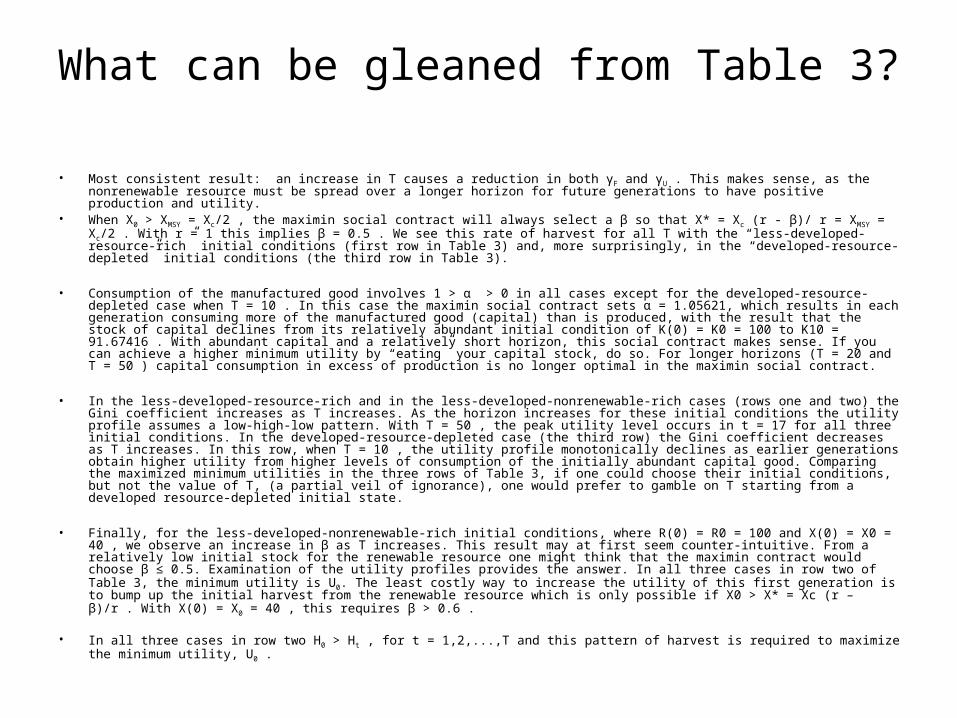
• Most consistent result: an increase in T causes a reduction in both γF and γU . This makes sense, as the nonrenewable resource must be spread over a longer horizon for future generations to have positive production and utility.

• When X0 > XMSY = Xc/2 , the maximin social contract will always select a β so that X* = Xc (r - β)/ r = XMSY = Xc/2 . With r = 1 this implies β = 0.5 . We see this rate of harvest for all T with the “less-developed-resource-rich” initial conditions (first row in Table 3) and, more surprisingly, in the “developed-resource-depleted” initial conditions (the third row in Table 3).

• Consumption of the manufactured good involves 1 > α > 0 in all cases except for the developed-resource-depleted case when T = 10 . In this case the maximin social contract sets α = 1.05621, which results in each generation consuming more of the manufactured good (capital) than is produced, with the result that the stock of capital declines from its relatively abundant initial condition of K(0) = K0 = 100 to K10 = 91.67416 . With abundant capital and a relatively short horizon, this social contract makes sense. If you can achieve a higher minimum utility by “eating” your capital stock, do so. For longer horizons (T = 20 and T = 50 ) capital consumption in excess of production is no longer optimal in the maximin social contract.

• In the less-developed-resource-rich and in the less-developed-nonrenewable-rich cases (rows one and two) the Gini coefficient increases as T increases. As the horizon increases for these initial conditions the utility profile assumes a low-high-low pattern. With T = 50 , the peak utility level occurs in t = 17 for all three initial conditions. In the developed-resource-depleted case (the third row) the Gini coefficient decreases as T increases. In this row, when T = 10 , the utility profile monotonically declines as earlier generations obtain higher utility from higher levels of consumption of the initially abundant capital good. Comparing the maximized minimum utilities in the three rows of Table 3, if one could choose their initial conditions, but not the value of T, (a partial veil of ignorance), one would prefer to gamble on T starting from a developed resource-depleted initial state.

• Finally, for the less-developed-nonrenewable-rich initial conditions, where R(0) = R0 = 100 and X(0) = X0 = 40 , we observe an increase in β as T increases. This result may at first seem counter-intuitive. From a relatively low initial stock for the renewable resource one might think that the maximin contract would choose β ≤ 0.5. Examination of the utility profiles provides the answer. In all three cases in row two of Table 3, the minimum utility is U0. The least costly way to increase the utility of this first generation is to bump up the initial harvest from the renewable resource which is only possible if X0 > X* = Xc (r – β)/r . With X(0) = X0 = 40 , this requires β > 0.6 .

• In all three cases in row two H0 > Ht , for t = 1,2,...,T and this pattern of harvest is required to maximize the minimum utility, U0 .

Conclusions

• The model lead to an operational definition of the Rawlsian “social contract.” The social contract became a vector of rates of consumption, harvest, extraction for production of the manufactured good and extraction for direct utility. It was a social contract because it was adopted by all generations.

• The maximin social contract maximized the minimum generational utility over the horizon t = 0,1,...,T .

• While an analytic solution for the maximin social contract was not possible, the problem could be programmed on an Excel spreadsheet and easily solved for modest values of T .

• Is there anything to be learned from this simple model? Perhaps.

• When adding a renewable resource to the maximin problem, if there is no cost to harvest and if X0> XMSY , the maximin social contract would move the resource stock to the level that supports maximum sustainable yield. This adjustment takes place in t = 0 where H0 = (X0 ! XMSY ) and then Xt = XMSY and Ht= HMSY for t ! 1 regardless of the value for T .

• If X 0 < XMSY the harvest rate β may be greater than the rate associated with maximum sustainable yield if it is the least-cost way to increase Min Ut = U0 .

• Does the finite horizon in this computational model diminish it relevance. I think not. The difficulty with making sustainable choices when one cares about future generations is that we don’t know the stocks that future generations will find essential or desirable. We don’t know the preferences of future generations nor the technologies which will influence the value of manufactured or natural capital in the future.

• Uncertainty about preferences and technology make maximin over an infinite horizon an elegant exercise of questionable relevance. It may be better to build finite-horizon models with greater reality in their economic and resource structure and explore, computationally, maximin in greater detail.

References d´Autume, A. and K. Schubert. 2008. “Hartwick’s Rule and Maximin Paths when the Exhaustible Resource has Amenity Value,” Journal of Environmental Economics and Management, 56(3) 260-274.

Hartwick, J. M. 1977. “Intergenerational Equity and the Investing of Rents from Exhaustible Resources,” American Economic Review, 66(5):972-974.

Rawls, J. 1971. A Theory of Justice, Harvard University Press, Cambridge.

Solow, R. M. 1974. “Intergenerational Equity and Exhaustible Resources,” Review of Economic Studies (Symposium on the Economics of Exhaustible Resources), 29-45.

Withagen, C and G. B. Asheim. 1998. “Characterizing Sustainability: The Converse of Hartwick’s Rule,” Journal of Economic Dynamics and Control, 23:159-165.