max planck institute for dynamics and self-organization
TRANSCRIPT

arX
iv:1
610.
0694
2v3
[co
nd-m
at.d
is-n
n] 9
Jan
201
8
Modes of failure in disordered solids
Subhadeep Roy1,2,∗ Soumyajyoti Biswas3,† and Purusattam Ray1‡1 The Institute of Mathematical Sciences, Taramani, Chennai-600113, India.
2 Earthquake Research Institute, University of Tokyo, 1-1-1 Yayoi, Bunkyo, 113-0032 Tokyo, Japan.3 Max Planck Institute for Dynamics and Self-Organization, Am Fassberg 17, Gottingen, Germany.
(Dated: August 4, 2021)
The two principal ingredients determining the failure modes of disordered solids are the strength ofheterogeneity and the length scale of the region affected in the solid following a local failure. Whilethe latter facilitates damage nucleation, the former leads to diffused damage – the two extreme natureof the failure modes. In this study, using the random fiber bundle model as a prototype for disordersolids, we classify all failure modes that are the results of interplay between these two effects. Weobtain scaling criteria for the different modes and propose a general phase diagram that providesa framework for understanding previous theoretical and experimental attempts of interpolationbetween these modes. As the fiber bundle model is a long standing model for interpreting variousfeatures of stressed disordered solids, the general phase diagram can serve as a guiding principle inanticipating the responses of disordered solids in general.
I. INTRODUCTION
Response of a disordered solid subjected to stress pro-vide a vital route in predicting imminent breakdown inthose systems. Understanding such responses is a ma-jor goal for myriads of situations starting from micro-fracture to earthquakes [1]. The apparent independenceof the effect of the structural details in the static anddynamic responses of the disordered solids, for exampleroughness of a fractured front, avalanche size distribu-tions etc., fueled decades of efforts in modeling thesephenomena using simple, generic and minimal ingredi-ents [2]. The focus of these studies is on the understand-ing of the mechanical stability of the systems, precursorto catastrophic failure and also to explore the possibilityof universality of the above mentioned response statisticsin the sense of critical phenomena. However, while therecan be scale free behavior of response functions indicat-ing criticality in some cases, there can also be nucleationdriven abrupt failures in others. Therefore, such associ-ation of fracture with critical phenomena is not straightforward (see e.g. [3, 4]).It is, however, known that the two main factors that
determine such modes of failures are the strength of dis-order and the range of interaction within the solid interms of stress transfer. The aim of this work is to clas-sify all the phases arising out of the interplay of thesetwo effects and to arrive at criteria in distinguishing suchphases, thereby providing a framework for understand-ing all the modes of failure using a simple model for thedisordered solids.It is known experimentally that the presence of hetero-
geneity increases the precursory signals prior to failure[5]. The strain energy is dissipated within a short rangeof crack propagation in heterogeneous solids, as opposed
∗ [email protected]† [email protected]‡ [email protected]
to those lacking heterogeneity. Strong heterogeneities,therefore, compel the system transit from a brittle liketo a quasi-brittle like failure mode [6]. Such a transi-tion in porous media was observed in Ref. [7], while thedisorder (porosity) spanned two decades in magnitude.The apparent contradiction of scale free size distributionfor acoustic emission and subsequent damage nucleationwas also observed in Ref. [8]. While experimentally it isnot easy to tune the strength of disorder precisely, heattreatment can tune the length scale of disorder in phase-separated glasses [9]. There have been many other exper-iments and simulations describing the effect of increaseddisorder on roughness [10], pattern formation in springnetworks [11, 12], damage nucleation and percolation inrandom fuse models [13, 14] etc.
As for the range of stress redistribution, linear elasticfracture mechanics predict a 1/r2 type load redistribu-tion around an Inglis crack [15, 16]. However this formis not always guaranteed and can change due to finitewidth of the sample [17], correlation in disorder [18], sizeof agglomerate [19] and so on. Here we attempt to charac-terize the formation of spatial and temporal correlationarising out of the interplay of the stress redistribution,which enhances damage nucleation, and the presence ofdisorder, which leads to diffused damage [20–22].
In this work, we report a phase diagram in the stressredistribution range and strength of disorder that cap-tures all failure modes arising out of the interplay be-tween these two. We consider the fiber bundle model[2, 23], which has been widely used as a generic model forfracture in disordered system over many years. Amongthe many modeling approaches that attempt to capturethe statistics of failure of disordered solids, fiber bundlemodel is arguably the simplest. Introduced in the textileengineering [24], it has been proven very useful in repro-ducing behaviors near failure [2]. The avalanche statisticsand also the roughness of fracture propagation front aris-ing out of its intermittent dynamics, compares favorablywith experiments [25]. The model is a set of elements ar-ranged in a lattice, each having a finite failure threshold

2
drawn randomly from a distribution. On application ofload, the elements —fibers — fail irreversibly and redis-tribute their load in a pre-defined neighborhood.
The two main ingredients of the model are the afore-mentioned neighborhood of load redistribution and thestrength of the disorder in the failure thresholds of theindividual fibers. The two extreme ways of defining theneighborhood are the equal and local load sharing mod-els. In the former, the load of a broken fiber is sharedequally among all the remaining intact fibers and in thelatter, it is shared only with its nearest surviving neigh-bors. Neither of these two extremes are realistic, howeverthey are important in establishing limiting behaviors ofthe model. Particularly, for local load sharing, the localstress concentration around damage is so high that thefailure statistics is governed by extreme statistics [26–29]and the critical load for the system decreases with systemsize [30, 31]. On the other hand, a global load sharingmodel gives a finite failure threshold, as the stress concen-tration is much lower here. Other than the two extremes,there has been a lot of studies that attempt to capture amore realistic way of redistributing the stress. An obvi-ous candidate was power-law load sharing [32], where theexponent of the power law determines the localization ofstress, which we will discuss later. Among other more re-alistic attempts was the one by Hedgepeth and Van Dyke[33], applied for polymer matrix composites. While therecan be situations such as plastic deformation, highly non-linear effects nea the crack-tip in the above examples,where a simple redistribution rule is no longer valid, herewe limit ourselves to the smooth asymptotics describedby a power law load sharing. The asymptotic form of theHedgepeth load sharing rule, however, is inverse cubicfor two-dimensions [34]. More detailed load sharing rulesinclude those proposed by Okabe et al. among others [35–38]. Particularly, as plastic and interfacial damages areconsidered, the load sharing for these cases interpolatebetween global and Hedgepeth load sharing. Further-more, there are time dependent load sharing rules [39, 40]that also interpolate between local and global load shar-ing. Therefore, a substantial literature in physics andengineering community has been developed in addressingthe question of load redistribution range and their effecton stress localization and ultimately the failure thresholdof the materials, using the fiber bundle model.
On the other hand, the disorder in the model comesfrom the distribution of the failure threshold. The prop-erties of the distribution function can influence the stresslocalization, and that, in turn, can determine the fail-ure strength of the system. The spread of damage andthe crackling noise, which can be used as a pre-cursor tocatastrophic failure, is significantly affected by the pres-ence of disorder. Particularly, higher disorder increasesthe pre-cursory events in the solids [5]. Due to its im-portance, there have been many efforts in looking for theeffect of disorder strength was made on the fiber bundlemodel [41, 42]. Particularly in the global load sharingcase, the effect of high disorder in known to bring the
system from brittle to quasi-brittle state [43].
Using the simplicity and flexibility of the fiber bun-dle model, we can tune both the strength of disorder andstress redistribution range and obtain the different phasesof failure in the fiber bundle model by varying the rangeof stress redistribution and strength of disorder. Withthe help of the phase diagram, we can now identify all itsmodes of failure, classify previous attempts to interpo-late between some of those modes and most importantlyarrive at scaling prescriptions in categorizing and predict-ing such failure modes. The scaling prescriptions differfrom their equilibrium, and often intuitive, counterparts(say, in Ising model), making them interesting also fromthe point of view of critical phenomena.
II. MODEL & SIMULATION
Here we simulate the failure in fiber bundle model inone and two dimensions – the one dimensional case isan idealized but the simplest one, while the two dimen-sional case is more realistic and has been used to modelfailure in fibrous materials (e.g. fiber reinforced com-posites) for many years [26–29]. We choose the failurethresholds of the fibers from a distribution of the formp(x) ∼ 1/x within a range [10−β : 10β]. For high valuesof β, the distribution becomes very broad, making thesystem a highly disordered one. Physically, this impliesvarying strength of impurities in the system, that cansignificantly influence the overall critical strength of thesystem. Following the failure of a fiber, the load on thefailed fiber is redistributed uniformly up to a distance R.In one dimension, this is simply R surviving neighboringfibers on either side of the failed one. In two-dimensionswe search along positive and negative x and y axes andgo up to a distance x+, x−, y+ and y− until R surviv-ing neighbors are found along each direction (see Fig.1). We then redistribute the load within the rectangularregion (x+, y+), (x−, y+), (x−, y−), (x+, y−) (assumingthe origin at the failed fiber). Of course, there can beother choices, for example a circular region of radius R.While that could work well for higher values of R, butfor smaller values there could be situations where therewere no surviving fibers within that region. Moreover,such details are unlikely to affect the scaling behavior,which is also evident from the fact that our predictionmatches well with power-law load redistribution studiedin Ref. [32].
With changes in these two parameters (β and R) weget the different failures modes of the model. We willfirst describe the phase diagram to explain the differ-ent modes. Subsequently we will discuss the methodsof drawing the boundaries and relate them to previousnumerical and experimental attempts of interpolations.

3
FIG. 1. The load redistribution region for a finite range R isshown for the one dimensional and two dimensional version ofthe model. The intact fibers in the shaded region (denoted byfilled circles) are affected by the load redistribution following afailure of a fiber (denoted by a cross), while the empty dottedcircles are broken fibers and empty circles outside the regionare sites of fibers that are not affected by this event. For amore general power law load redistribution (not shown), how-ever, all intact fibers are affected but the shared load variesinversely with the distance from the broken fiber.
III. NUMERICAL RESULTS
Numerical results are produced for different systemsizes over a wide range disorder and stress release range.Six different regions are observed through numerical sim-ulations with individual modes of failure.
A. The R − β Plane
Intuitively, we expect a nucleating failure for low valuesof R and β. This resembles brittle failures of perfectlycrystalline structures. The failure thresholds of each partof the system are almost same, therefore an initial failureand subsequent load concentration around it (due to lowR values) compels the subsequent damages to be nearthat initial damage and it will continue to grow. Thussmall R and β imply high spatial correlation in dam-age. This damage nucleation can be prevented by eitherredistributing the load of a failed fiber to a relativelylarge distance, or by increasing the disorder such thatthe nearby fiber can have high failure threshold whichcompels distant fibers to fail first.On the other hand, higher the number of fibers break-
ing due to stress redistribution, higher is the temporal
1000
3000
5000
7000
0.1 0.3 0.5 0.7 0.9 1.1
R
β
B
D
A
C
E
(a) 1d Model
F
10
30
50
0.6 1.2 1.8
R
β
B
D
A
C
E
(b) 2d Model
F
FIG. 2. The figure shows all the regions on R − β plane for:(a) 1d and (b) 2d bundle. B and D are brittle regions andshow abrupt failure. A and C show quasi-brittle response.Only difference is, in region A and B rupture process is spa-tially correlated. In region E (spatially uncorrelated) and F(spatially correlated), the failure process is mainly dominatedby stress increment.
correlation (we will present quantitative measures later).The temporal correlation in damage, i.e. avalanches, alsobehave similarly with R and β. Small R and β implyhigher correlation. The difference is that the temporalcorrelation does not vanish at the same values of R andβ, as the spatial correlation. The phase diagram (Fig.2), therefore, has regions where temporal correlation ex-ists without spatial correlation, hence giving interestingphases for the model.
B. Description of the Phases
Below we first describe each of the phases depictedin Fig.2 and then describe the quantitative measures fordrawing the boundaries between the phases.

4
1. B: Brittle-nucleating
In this region, as soon as the weakest fiber is broken,the entire system collapses starting from damage nucle-ation happening next to the failed fiber. This is a brittlelike failure (like in ceramics, say) and have both temporaland spatial correlations. The avalanche is a catastrophicfailure here, with size ∼ L.
2. D: Brittle-percolating
The system here also collapses following the breakingof the weakest fiber, but as R is large enough, the sub-sequent damage is spatially uncorrelated i.e. multipledamage nucleation zones are formed.
3. A: Quasi-brittle nucleating
In this region, the system fails after multiple stablestates, hence the nature of failure is quasi-brittle. In thisregion, an apparent random failure eventually forms aspatially correlated failure i.e. the system begins with ascale free avalanche distribution, but for larger systemsthe final failure is nucleation driven (see reference [44, 45]for electrical analogue).
4. C: Quasi-brittle percolating
This is the region where the R and β combination issuch that although the spatially correlation has vanished,the temporal correlation exists. This is the region withscale free size distribution (exponent −5/2 [2]) of theavalanches.
5. E: High disorder limit
In this region, neither the spatial correlation nor thetemporal correlation exists. As can be seen, this regionappears even for very low R values, given the disorderdistribution is broad enough (high β).
6. F: Temporally uncorrelated region
In this region the temporal correlation in rupturingfibers vanishes. Since the spatial correlation still exists,the failure happens in a nucleating manner.
C. Visualizing the failure modes
Before we go to the description of the methods fordrawing the phase boundaries, let us first look at the var-
ious failure modes described above. The temporal con-figurations of the damages and stress profiles can give aqualitative idea of the different modes, which we will laterdescribe in the quantitative forms. In one dimension, it is
FIG. 3. The configurations of the failures in one dimensionfor different values of R and β. The x-axis is time and y-axis is the whole system. Zero stress imply broken fibers.For different values of the parameters nucleation phenomenoncan be clearly seen. The difference between the avalancheand percolative failures are not apparent from the snap-shot,which will become clearer with the quantitative analysis inthe following section.
easier to see the full temporal evolution of the damagesand stress concentrations. In Fig. 3 we plot the timeevolution of the model for different ranges of the R, βparameters. The x-axis is the time, and in the y-axisthe temporal stress profiles of the system is shown, zerostress imply broken fibers. For low values of β and R, wesee clear nucleation, which eventually engulfs the wholesystem. For slightly higher values, we see initial randomfailures, but in time a nucleation center grows, till thewhole system collapses. For high values of β and R, onthe other hand, there is no nucleation, and the damageprofile is rather random in space. For this qualitative pic-ture, it is not possible to see the distinctions between thetemporally correlated failures for high R and intermedi-ate β values, and the percolative failure for very high βvalues. For that we need to look at the more quantita-tive measures described below. But this gives a pictorialsense of the damage profile and the dynamics prior tofailure in the model for different ranges of values of Rand β.In two dimensions, it is harder to see the temporal
effects for obvious reasons. Nevertheless, in Fig. 4 weplot the stress/damage profile of the system for variousmodes of failures. The horizontal axis is snaps at differenttimes. Vertically from top to bottom we show the failuresmodes of avalanche, percolation, brittle and nucleation.It is to be noted that the snaps are not in equal timeintervals. In the avalanche process, we see that there isno spatial correlation of the damages and the stress pro-

5
FIG. 4. The different modes of failures for two-dimensionsare shown in terms of the stress profile at various times priorto failure in a 100 × 100 lattice, for different R and β val-ues. The black regions are broken fibers. From top to bot-tom the modes are avalanche, percolative, brittle and nucle-ating. Along horizontal axis snaps for different time stepsare shown. The times are not equispaced for different modes.In the avalanche mode (γ = −1.0, β = 0.6), the time stepsshown are 415, 568, 630 and 676. For the percolating region(γ = −6.0, β = 2.5), the steps are 83, 199, 269, 385. Forthe brittle region (γ = −3.0, β = 0.1) 99, 100, 101, 102. Fi-nally, for the nucleation mode (γ = −6.0, β = 0.5), the timesteps are 92, 165, 203 and 215. The stress profiles and dam-age configurations give a qualitative idea about the differentfailure modes. For the avalanche mode in the top, there is nospatial correlation in damage and the stress profile is moreor less uniform. The similar feature can also be seen for thepercolative failure, but in general with higher stress due tohigher disorder. For the brittle failure the stress is uniformtoo and the failure is very abrupt. For the nucleation, a stressconcentration in the spatially correlated damage region canclearly be seen.
files are more or less uniform. In the percolation processtoo, there is no spatial correlation in damage, but thestress values here goes to much higher values, since thedisorder in very high and there are many strong fibers.The principal distinction between the brittle region andthe nucleation region is in the time scales. While in thebrittle region the snaps are unit time step apart, in thenucleation regions they are much further apart. It showsthat in the brittle region the whole system collapse sud-denly. On the other hand, in the nucleating region, theinitial damages were random. But at later times onedamaged area starts growing, due to the high stress con-centration at its boundary, which can also be clearly seen.This gives a qualitative idea about the phases of failures,which we will now discuss more quantitatively in termsof the phase boundaries.
D. Description of the Phase Boundaries
The various phases described above are separated byphase boundaries drawn on specific criteria. We will de-scribe those now.
1. Quasi-brittle percolating (A) − quasi-brittle nucleating(C) boundary
A general way to determine spatial correlation is tomonitor the cluster density with fraction of broken fibers.Fig. 5 shows the variation of cluster density np (numberof cluster divided by system size) with fraction of bro-ken bonds 1 − U , at different R and β values, for bothone and two dimension. In one dimension, the numberof clusters of broken fibers is simply the number of sideby side broken and unbroken fibers present. If U is thefraction of surviving fibers at any time, then for com-plete random failure, the number of side by side bro-ken and unbroken fiber will be U(1 − U) (normalizedby system size). Any deviation of np from this func-tion would indicate spatial correlation. A quantitativemeasure for such departure is the area under this np v/s(1 − U) curve and compared it with the situation whenthe rupture is completely uncorrelated. In case of un-correlated failure (for high R or β) the area under the
curve will be A1d =
∫ 1
0
U(1 − U)dU = 1/6. At low R
and β, the area under the curve deviates from A1d. Fortwo dimensions the situation is qualitatively similar. Butthe general shape of the curve for random failure is notknown. However, there are many numerical studies interms of random site percolation (see Ref. [46] and ref-erences therein) that looks at density of patches underrandom occupations (see Fig.5).
The deviation of the np v/s 1 − U curves from therandom case determines this boundary. This gives acrossover scale Rc, which scales with the system size asL2/3 [47] in one-dimension. In two dimension the scalingchanges to
Rc ∼ Lb, (1)
with b = 0.85± 0.01. Fig.6 shows the scaling of Rc withsystem size L in a two dimensional fiber bundle model.The areas (A2d) under np vs 1−U curves (see Fig.5) fordifferent L values are observed to scale with RL−b, whereb = 0.85.
One interesting implication of the scaling is, when theload sharing is a power law, the effective range of the loadredistribution can be shown to be Reff ∼ L3−γ , whereγ is the power of the load redistribution process. Thiscan be understood through following calculation. Withpower law redistribution rule an effective range can be

6
0
0.1
0.2
0 0.4 0.8
n p
1-U
(d)
β=0.5
R=5R=50
R=100
0 0.4 0.8
1-U
(e)
β=0.9R=1
R=10R=100
0 0.4 0.8
1-U
(f)
β=4.0
R=1R=10
R=100
0
0.1
0.2
n p(a)
R=1
β=0.8β=2.0β=4.0
(b)R=10
β=0.5β=1.0β=2.0
(c)
R=200
β=0.5β=2.0β=4.0
0
0.05
0.1
0 0.4 0.8
n p
1-U
(d)
β=0.5
R=1R=5
R=10R=30rand
0 0.4 0.8
1-U
(e)
β=1.0
R=1R=5
R=10R=30rand
0 0.4 0.8
1-U
(f)
β=4.0
R=1R=5
R=30rand
0
0.05
0.1
n p
(a)
R=1
β=0.5β=0.7β=1.0β=4.0rand
(b)
R=5
β=0.5β=0.7β=1.0β=4.0rand
(c)
R=30
β=0.5β=1.0β=4.0rand
FIG. 5. The variations of number of patch per fiber (np) areshown for constant range (R) and different strength of disor-der β [(a-c) for one dimension and (d-f) for two dimension]and for constant strength of disorder and different ranges [(g-i) for one dimension and (j-l) for two dimension] with fractionof broken fibers (1− U). It can be seen that for both high Rand high β values, the curves merge with the ones obtained forcompletely random failures. The two limits, however, differin term of dynamics, as discussed in the text.
defined as:
Reff = 〈r〉 =
L∫
1
rP (r)2πrdr =2− γ
3− γ
L3−γ − 1
L2−γ − 1, (2)
where P (r) ∼ 1/rγ . For γ < 2, Reff ∼ L, implyingmean-field regime. Also, for γ > 3, Reff ∼ const., there-fore it is always local load sharing type. However, for2 < γ < 3, Reff ∼ L3−γ in the large system size limit.Since Rc ∼ Lb, to get the crossover value for γ we haveto compare Reff (γc) ∼ Rc, giving
γc = 3− b. (3)
But b < 1(= 0.85), giving γc > 2(2.15). This explainsan apparent result for γc > 2 [32], which can now beclaimed with much higher numerical accuracy. To ver-ify this point, we have performed numerical simulations
0.054
0.056
0.058
0.06
0.062
0.064
0.066
0.068
0 0.05 0.1 0.15 0.2 0.25 0.3 0.35 0.4
Are
a (A
2d)
R/Lb
b=0.85
b=1
L=100L=200L=300L=400L=800
0.054
0.058
0.062
0.066
0 20 40 60 80 100
Are
a (A
2d)
R
L=100L=200L=300L=400L=800
FIG. 6. For the two dimensional model, the scaling of the areaunder the patch density versus fraction of failed fibers curves(shown in Fig. 5) with R are shown. The linear scaling inthe x-axis does not show satisfactory data collapse. The bestcollapse is seen when b = 0.85. The unscaled data are shownin the inset.
20
30
40
50
60
70
80
90
100
110
1.4 1.6 1.8 2 2.2 2.4 2.6
m2/
m1
γ
L=200L=300L=800
L=200, β=0.5L=300, β=0.5
FIG. 7. The moment ratios of the cluster size distribution ofthe broken fibers in a two-dimensional power-law load sharingfiber bundle model are shown for different system sizes withγ. The peaks are consistently at γ > 2. The threshold dis-tributions are either uniform, or power-law with β dependentcut-off, as mentioned.
with power-law load redistribution. We have studied thecluster statistics of the broken fibers in the final stableconfiguration prior to complete failure (as was done in thepaper by Hidalgo et al [32]). We measured the momentsof the cluster size distributions n(s). The k-th momentis defined as
mk =
∫skn(s)ds (4)
We have plotted the moment ratio m2/m1 in Fig.7. Thepeaks of the curves occur consistently above γ = 2 fordifferent system sizes and threshold distributions.

7
2. Brittle nucleating(B) − brittle percolating (D) boundary
The nature of this crossover line is the same as be-fore and is drawn by monitoring the cluster density. Thecrossover length scale Rc now scales non-universally withL, as Rc ∼ Lζ with ζ = ζ(β) [48].
3. High disorder nucleating (F) − high disorder percolating(E) boundary
This boundary is also drawn from the same measure asB-D boundary but the crossover scale here is independentof the strength of the disorder (Rc ∼ L2/3).
4. Brittle percolating (D) − quasi-brittle percolating (C)boundary
This class of boundaries separate brittle to quasi-brittle transitions. Particularly, in the brittle region, thebreaking of the weakest fiber will cause the breakdownof the entire system. Hence, by measuring the fractionof surviving fibers in the last stable configuration be-fore breakdown (Uc), we track the transition from brittle(with Uc = 1) to quasi-brittle (with Uc < 1) region. Aphase transition occurs only across this line [43, 49–51],with no system size dependence of the transition line.
5. Brittle nucleating (B) − quasi-brittle nucleating (A)boundary
This boundary is also drawn with the same criterionthat leads to the D-C boundary. There is, however, asystem size dependence of the line and it gets shifted tohigher β value with increasing system size in a inverselogarithmic manner (see Ref.[52]), for a particular stressrelease range.
6. Quasi-brittle percolating (C) − high disorder percolating(E) boundary
This boundary separates the completely uncorrelatedphase from temporally correlated quasi-brittle region C.We evaluate it in two different ways and the results matchfor the two cases. Fig.8 shows the behavior of averageavalanche size 〈s〉 in the mean filed limit against disor-der β and for system sizes ranging in between 103 and104. We have also discussed the scaling of the averageavalanche size 〈s〉 ∼ Lξ (see Fig.9). In the quasi-brittleregion, ξ is a (decreasing) function of β and eventually〈s〉 becomes independent of L in the high disorder limitE. The β value at which 〈s〉 becomes system size inde-pendent gives the boundary between C and E, becausesystem size independence signifies complete removal ofcorrelation in the system.
10-1
100
101
102
103
104
10-1 100 101
<s>
β
TemporallyUncorelated
TemporallyCorelated
D C Eβ1 β2 β*
L=1000L=3000L=5000
L=10000
FIG. 8. The variation of average avalanche size 〈s〉 with dis-order for different L values (in the mean-field limit). Middle:〈s〉/L vs β for 103 < L < 104.
0 0.2 0.4 0.6 0.8
1 1.2
0 0.2 0.4 0.6 0.8 1 1.2 1.4
ξ
β
(b) R=100R=1
100
101
102
103
104
105
102 103 104 105
<s>
L
(a) R=100β=0.1β=0.2
β=0.25β=0.27
β=0.3β=0.4β=0.5
FIG. 9. (a) System size effect of 〈s〉 at various disorder valuesfor for a particular stress release range (say R = 100). 〈s〉 ∼Lξ, where ξ is decreasing function of β. (b) ξ as a function ofdisorder β.
Different regions, according to Fig.8, is described below(see Fig.9 in support of the following behavior):
(i) For β < β1, the failure process is brittle like abrupt.〈s〉 ∼ L, since all the fibers break in a singleavalanche.
(ii) For β1 < β < β2, 〈s〉 ∼ Lξ, where ξ is an decreas-ing function of β and reaches to a very low value atβ2 (shown in main text). In this region the bundlebreaks in many avalanches like quasi-brittle mate-rial.
(iii) For β2 < β < β∗, 〈s〉 = k(> 1). Here k is func-tion of β only and independent of L. Very fewavalanches are observed in this region.

8
1.1
1.2
1.3
1.4
1.5
1.6
1.7
1.8
0 10 20 30 40 50 60 70 80 90 100
β*
R
L=104
<s> = 1
<s> > 1
FIG. 10. Behavior of β∗ with stress release range R. In thegreen region, there is no temporal correlation between therupturing fibers.
-20
-10
0
10
20
30
40
50
60
-150 -100 -50 0 50 100 150
(Ns-N
r)L
-α
[β-β2(L)]Lγ
(c)
α = γ = 1/2
R>Rc
L=105
L=5x10⁴
L=104
L=103
-50000
50001000015000
0.1 0.3 0.5 0.7 0.9
(Ns-N
r)
β
(d)
0
2000
4000
0.1 0.3 0.5 0.7 0.9
Ns
or
Nr
β
(a) Ns
Nr
β2(R>Rc)
R=500R=700
R=1000
10-2
10-1
103
104
105
[β2(L
)-β
2(∞
)]
L
R>Rc
(b)
L-1/2
FIG. 11. (a) Variation of Ns and Nr as a function of β forL = 104. (b) System size effect of β2, as the model approachesthermodynamic limit. (c) System size scaling of (Ns − Nr)around β = β2. The inset shows the unscaled behavior.
(iv) The green vertical line (see Fig.8), drawn at β =β∗, shows an extreme limit of temporal correlation.The variation of β∗ with R is shown in Fig.10. Withhigh local stress concentration (low R value), β∗
is around 1.7. With increasing R, as the modelentires the mean-field limit, β∗ saturates at 1.3. Inthe region β > β∗, the fibers break only by stressincrement, giving 〈s〉 = 1.
A second way to approach the problem is to measurethe number of stress increment Ns and the number of
times Nr stress were redistributed during the entire timeof survival of the system. Such interplay of Ns and Nr
is shown in Fig.11. When Ns outruns Nr, i.e. morefibers break due to stress increment (without spatial ortemporal correlations) than due to stress redistributions,the uncorrelated region E is obtained. We find that thedisorder strength β2 when this happens scales with thesystem size as: β2(L) = β2(∞) + L−α, with α = 1/2(see Fig.11). Also, the system size scaling of (Ns − Nr)is given by
(Ns −Nr) = LαΦ[(β2 − β2(L))Lγ ], (5)
with α = γ = 1/2. The β2 obtained in this way matcheswith the boundary obtained from the scaling of the aver-age avalanche size before. Hence we conclude that β2 isthe range of disorder beyond which the system becomescompletely uncorrelated (region E).
-200
-100
0
100
200
300
400
500
600
-150 -100 -50 0 50 100 150
(Ns-
Nr)
(L2d
)-α2d
[β-β2(L)](L2d)γ2d
(c)
α2d=γ2d=1
L2d=300
L2d=200
L2d=100
L2d=50
-60000-20000 20000 60000
0.2 0.5 0.8
(Ns-
Nr)
β
(d)
0
10000
20000
30000
40000
0.2 0.5 0.8
Ns
or N
r
β
(a) NsNr
β2(R>Rc)
R2d=20R2d=30R2d=50
10-2
10-1
102
[β2(
L 2d)
-β2(
∞)]
L2d
R>Rc
(b)L-1
FIG. 12. System size effect of β2 for different stress releaserange, for two dimensional model. (a) Variation of Ns and Nr
as a function of β for L = 102. (b) System size effect of β2,as the model approaches thermodynamic limit. (c) Systemsize scaling of (Ns −Nr) around β = β2. The inset shows theunscaled behavior.
Fig.12 shows this system size scaling of (Ns − Nr) inthe two dimension. The scaling shown in 5, holds thesame in two dimension also with respective exponentsα2d = γ2d = 1. This in turn establish the scaling of β2
as: β2(L) = β2(∞) + 1/L.

9
7. Quasi-brittle nucleating (A) − high disorder nucleating(F) boundary
This boundary is drawn with the same criterion usedto draw the boundary between C and E. Across thisboundary the temporal correlation vanishes but thespatial correlation still exists. At a certain stress release
100
103 104 105
β 2
L
L-0.06
L0.0
L0.07
R=1R=10
R=100
FIG. 13. System size effect of β2 for different stress releaserange R.
range R, β2 is not being observed to change much whilewe alter the system size (see Fig.13). β2 shows a scalefree behavior with L but with an extremely low exponentthat suggest a very very weak system size dependence ofβ2.
Finally, using the criteria outlined above, we arrive atthe quantitative phase diagram for fiber bundle modelin one and two dimensions (see Fig.2). Almost all thestudies in fiber bundle model fall in some point of thisphase diagram. The most studied region being the regionC, which is also historically the earliest. Subsequentlyregion A was studied, which is qualitatively differentfrom region C in the sense that we no longer observescale free avalanche statistics here. We provide a scalingcriterion to separate these two regions.
IV. DISCUSSIONS AND CONCLUSION
In fracture of disordered solids, the two main factorsdetermining the mode of failures are the range of interac-tion and the strength of disorder in the solids. It is knownthat higher disorder produce higher precursory events [5]in a solid prior to failure, which is important in predict-ing catastrophic breakdowns. A transition from brittleto quasi-brittle modes of failure was observed both the-oretically (see e.g. [43, 53, 54]) and experimentally (seee.g. [7, 55]) where the strength of disorder played a ma-jor role. However, the range of interaction i.e. the regionaffected by the load redistribution following a local fail-
ure also plays a crucial role in determining the effect ofdisorder strength. Generally, the compliance of the solid,determined by its elasticity, effect of agglomerate sizes,correlation or plastic deformation etc. determines therange of interaction. A localized redistribution promotesstress/damage nucleation whereas the disorder promotesspreading of damage. It is the interplay between the twothat gives many interesting effects in length and timescales in various failure modes for fracture of disorderedsolids. In this work we have addressed the interplay ofthese two effects using a random fiber bundle model inone and two dimensions. In isolation some of the lim-iting cases were studied before. But the full range oflocalization of strength and width of the disorder distri-bution give various phases and boundaries across whichthe relative influence of these two competing effects vary.In particular, we recover by increasing the range of in-teraction, a region with no spatial correlation, where thetemporal correlation still exists (avalanche region C) thatsurvives in the large system size limit (see Eq. 1), whichwas absent in the random fuse model. In that model theeventual nucleation was always dominant in the large sys-tem size limit (equivalent of region A). Experimentally,of course such regions are observed for many decades(see [1] for detailed discussions). Furthermore, we arealso able to verify the unusual scaling of the interactionrange that leads to nucleation. The fact that γc > 2 inEq. 3 (b < 1) has interesting consequences particularlyfor fracture, given the inverse square interaction is usu-ally expected for elastic solids. The criteria for drawingdifferent phase boundaries and the size-scaling in each ofthose phases are summarized in forms of table in the Ap-pendix. It is also to be noted that the phase boundariessometimes have dependence on system size (see e.g. Eq.(1)), therefore appropriate finite size scaling needs to bedone (as are mentioned for applicable cases) in order totranslate the results into different system sizes.
There have been many studies over the years in inter-polating between various phases of the fiber bundle modeldescribed above. Among these, most efforts were con-centrated in interpolating between regions A and C, be-cause this region gives the critical interaction range belowwhich the eventual failure will be nucleation dominated,a much debated topic in fracture [4]. The crossover fromA to C was also accessed in Ref. [56] by tuning the elasticmodulus of the bottom plate of the model, which in turncontrols the range of interaction. In Ref. [43] the authorsmoved from region D to C in the mean-field limit. Thevalue of β was exactly calculated in the mean-field limit[49]. Similar transitions between D and C phases for ageneric class of disorder distribution was also noted inrefs.[50, 51].
Many experimental observations, like brittle (region B& D) to quasi-brittle/ductile (region A & C) transition[7], scale free size distribution for acoustic emission [8],subsequent damage nucleation [8] etc., can also be ex-plained by this phase diagram. Such properties are char-acteristic of region A, where the so called ‘finite size crit-

10
icality’ [45] is observed, i.e. the system starts off givingscale free avalanches, but the final failure is nucleationdriven. Unlike random resistor network [44], where nu-cleation always dominates in the final failure mode, in thefiber bundle model phase diagram, there exists a tempo-rally correlated failure mode that sustains in the thermo-dynamics limit.
In conclusion, we have obtained a phase diagram forfailure of disordered solids using random fiber bundlemodel. We describe all distinct modes of failure with
varying disorder (β) and stress release range (R). Dis-order effects the abruptness of the failure process whilethe stress release range influences the correlation betweensuccessive rupturing of fibers. Interplay of these two af-fects leads to spatial and/or temporal correlation or ran-dom failures. The resulting phase diagram gives a frame-work for understanding previous theoretical and exper-imental attempts to interpolate between these differentfailure modes.SB acknowledges Alexander von Humboldt foundation
for funding.
[1] B. K. Chakrabarti and L. G. Benguigui, StatisticalPhysics of Fracture and Breakdown in Disordered Sys-tems (Oxford University Press, Oxford, 1997); M.Sahimi, Heterogeneous Materials II: Nonlinear andBreakdown Properties (Springer-Verlag, New York,2003); S. Biswas, P. Ray, B. K. Chakrabarti, Statisti-cal physics of fracture, breakdown and earthquake (Wiley-VCH, July 2015).
[2] S. Pradhan, A. Hansen, B. K. Chakrabarti, Rev. Mod.Phys 82, 499 (2010).
[3] Y. Moreno, J. B. Gomez, A. F. Pacheco, Phys. Rev. Lett.85, 2865 (2000).
[4] S. Zapperi, P. Ray, H. E. Stanley, A. Vespignani, Phys.Rev. Lett. 78, 1408 (1997).
[5] J. Vasseur, F. B. Wadsworth, Y. Lavallee, A. F. Bell, I.G. Main, D. B. Dingwell, Sci. Rep. 5, 13259 (2015).
[6] T.-F. Wong, P. Baud, J. Struct. Geol. 44, 25 (2012).[7] R. Li, K. Sieradzki, Phys. Rev. Lett. 68, 1168 (1992).[8] A. Guarino, A. Garcimartin, S. Ciliberto, Eur. Phys. J.
B 6, 13 (1998).[9] D. Dalmas, A. Lelarge, D. Vandembroucq, Phys. Rev.
Lett. 101, 255501 (2008).[10] V. V. Silberschmidt, Int. J. Fract. 140, 73 (2006).[11] I. Malakhovsky, M. A. J. Michels, Phys. Rev. B 76,
144201 (2007).[12] P. Ray, G. Date, Physica A 229, 26 (1996).[13] P. K. V. V. Nukala, S. imunovi, S. Zapperi, J. Stat. Mech
2004 P08001 (2004).[14] B. Kahng, G. G. Batrouni, S. Redner, L. de Arcangelis,
H. J. Herrmann, Phys. Rev. B 37, 7625 (1988).[15] J. Schmittbuhl, S. Roux, J.-P. Vilotte, K. J. Maløy, Phys.
Rev. Lett. 74, 1787 (1995).[16] S. Ramanathan, D. Ertas, D. S. Fisher, Phys. Rev. Lett.
79, 873 (1997).[17] Z. C. Xia, J. W. Hutchinson, J. Mech. Phys. Solids 48,
1107 (2000).[18] C. K. Peng, S. Havlin, M. Schwartz, H. E. Stanley, Phys.
Rev. A 44, R2239 (1991).[19] K. Kendall, N. McN Alford, W. J. Clegg, J. D. Birchall,
Nature 339, 130 (1989).[20] W. A. Curtin, J. Mech. Phys. Solids 41, 217 (1993).[21] D. Amitrano, J. Grasso, D. Hantz, Geophys. Res. Lett.
26, 2109 (1999).[22] D. De Tommasi, G. Puglisi, G. Saccomandi, Phys. Rev.
Lett. 100, 085502 (2008).[23] A. Hansen, P. C. Hemmer & S. Pradhan, The Fiber Bun-
dle Model: Modeling Failure in Materials Wiley VCH
Berlin (2015).[24] F. T. Peirce, J. Text. Inst. 17, T355 (1926).[25] D. Bonamy, J. Phys. D 42, 214014 (2009).[26] D. G. Harlow, S. L. Phoenix, J. Composite Mater. 12,
195 (1978).[27] D. G. Harlow, S. L. Phoenix, J. Mech. Phys. Solids 39,
173 (1991).[28] S. L. Phoenix, Fibre Sci. and Tech. 7, 15 (1974).[29] S. L. Phoenix, Int. J. Engrg. Sci. 13, 287 (1975).[30] D. G. Harlow, Proc. R. Soc. London A 397, 211 (1985).[31] G. Dill-Langer, R. C. Hidalgo, F. Kun, Y. Moreno, S.
Aicher, H. J. Herrmann, Physica A 325, 547 (2003).[32] R. C. Hidalgo, Y. Moreno, F. Kun, H. J. Herrmann, Phys.
Rev. E 65, 046148 (2002).[33] J. M. Hedgepeth, P. V. Dyke, J. Compos. Mater. 1, 294
(1967).[34] A. Gupta, S. Mahesh, S. M. Keralavarma, Int. J. Fract.
204, 121 (2017).[35] T. Okabe, N. Takeda, Y. Kamoshida, M. Shimizu, W.
Curtin, Comp. Sci. Technol. 61, 1773 (2001).[36] T. Okabe, N. Takeda, Composites A 33, 1327 (2002).[37] A. Mishra, S. Mahesh, Int. J. Solids Struct. 121, 228
(2017).[38] A. Gupta, S. Mahesh, S. M. Keralavarma, Phys. Rev. E
96, 043002 (2017).[39] W. I. Newman, S. L. Phoenix, Phys. Rev. E 63, 021507
(2001).[40] S. L. Phoenix, W. I. Newman, Phys. Rev. E 80, 066115
(2009).[41] Z. Danku, F. Kun, J. Stat. Mech. 2016, 073211 (2016).[42] V. Kadar, Z. Danku, F. Kun, Phys. Rev. E 96, 033001
(2017).[43] S. Roy, P. Ray, EPL 112, 26004 (2015).[44] A. A. Moreira, C. L. N. Oliveira, A. Hansen, N. A.
M.Araujo, H. J. Herrmann, and J. S. Andrade, Jr., Phys.Rev. Lett. 109, 255701 (2012).
[45] A. Shekhawat, S. Zapperi, and J. P. Sethna, Phys. Rev.Lett. 110, 185505 (2013).
[46] R. M. Ziff, S. R. Finch, V. S. Adamchik, Phys. Rev. Lett.79, 3447 (1997).
[47] S. Biswas, S. Roy, P. Ray, Phys. Rev. E 91, 050105(R)(2015).
[48] S. Roy, S. Biswas, P. Ray, arxiv:1606:06062.[49] C. Roy, S. Kundu, S. S. Manna, Phys. Rev. E 91, 032103
(2015).[50] J. V. Andersen, D. Sornette, and K. T. Leung, Phys.
Rev. Lett. 78, 2140 (1997).
11
[51] R. daSilveira, Phys. Rev. Lett. 80, 3157 (1998).[52] Subhadeep Roy, arXiv:1707.02422 (2017).[53] E. Karpas, F. Kun, EPL 95, 16004 (2011).[54] S. Papanikolaou, J. Thibault, C. Woodward, P. Shan-
thraj, F. Roters, arXiv:1707.04332 (2017).[55] J. Scheibert, C. Guerra, F. F. Celarie, D. Dalmas, D.
Bonamy, Phys. Rev. Lett. 104, 045501 (2010).[56] A. Stormo, K. S. Gjerden, A. Hansen, Phys. Rev. E 86,
025101(R) (2012).
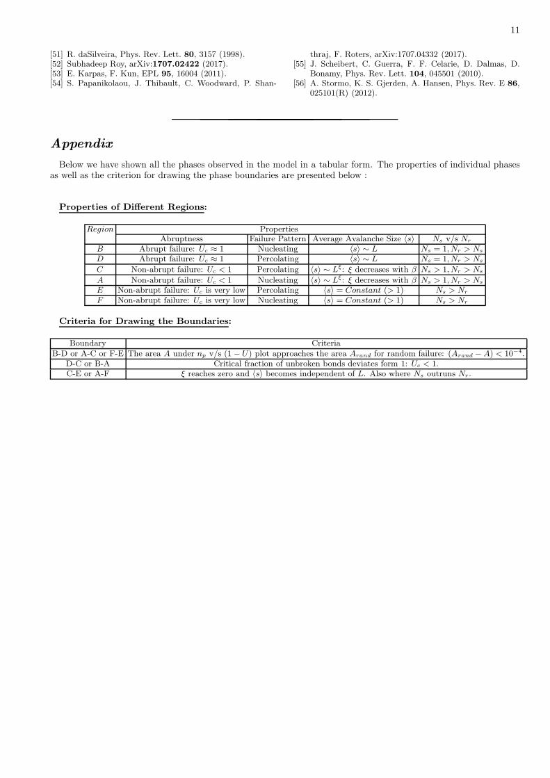
Appendix
Below we have shown all the phases observed in the model in a tabular form. The properties of individual phasesas well as the criterion for drawing the phase boundaries are presented below :
Properties of Different Regions:
Region PropertiesAbruptness Failure Pattern Average Avalanche Size 〈s〉 Ns v/s Nr
B Abrupt failure: Uc ≈ 1 Nucleating 〈s〉 ∼ L Ns = 1, Nr > Ns
D Abrupt failure: Uc ≈ 1 Percolating 〈s〉 ∼ L Ns = 1, Nr > Ns
C Non-abrupt failure: Uc < 1 Percolating 〈s〉 ∼ Lξ: ξ decreases with β Ns > 1, Nr > Ns
A Non-abrupt failure: Uc < 1 Nucleating 〈s〉 ∼ Lξ: ξ decreases with β Ns > 1, Nr > Ns
E Non-abrupt failure: Uc is very low Percolating 〈s〉 = Constant (> 1) Ns > Nr
F Non-abrupt failure: Uc is very low Nucleating 〈s〉 = Constant (> 1) Ns > Nr
Criteria for Drawing the Boundaries:
Boundary CriteriaB-D or A-C or F-E The area A under np v/s (1− U) plot approaches the area Arand for random failure: (Arand − A) < 10−4.
D-C or B-A Critical fraction of unbroken bonds deviates form 1: Uc < 1.C-E or A-F ξ reaches zero and 〈s〉 becomes independent of L. Also where Ns outruns Nr.