Noname manuscript No.(will be inserted by the editor)

Max Margin Learning of Hierarchical Configural Deformable Templates(HCDTs) for Efficient Object Parsing and Pose Estimation

Long (Leo) Zhu · Yuanhao Chen · Chenxi Lin · Alan Yuille

the date of receipt and acceptance should be inserted later

Abstract In this paper we formulate a hierarchical config-urable deformable template (HCDT) to model articulatedvisual objects – such as horses and baseball players – fortasks such as parsing, segmentation, and pose estimation.HCDTs represent an object by an AND/OR graph where theOR nodes act as switches which enables the graph topologyto vary adaptively. This hierarchical representation is com-positional and the node variables represent positions andproperties of subparts of the object. The graph and the nodevariables are required to obey the summarization principlewhich enables an efficient compositional inference algorithmto rapidly estimate the state of the HCDT. We specify thestructure of the AND/OR graph of the HCDT by hand andlearn the model parameters discriminatively by extendingMax-Margin learning to AND/OR graphs. We illustrate thethree main aspects of HCDTs – representation, inference,and learning – on the tasks of segmenting, parsing, and pose(configuration) estimation for horses and humans. We demon-strate that the inference algorithm is fast and that max-marginlearning is effective. We show that HCDTs gives state of the

Long (Leo) ZhuDepartment of StatisticsUniversity of California at Los AngelesLos Angeles, CA 90095E-mail: lzhu@stat.ucla.edu

Yuanhao ChenUniversity of Science and Technology of ChinaHefei, Anhui 230026 P.R.ChinaE-mail: yhchen4@ustc.edu

Chenxi LinAlibaba Group R&DE-mail: chenxi.lin@alibaba-inc.com

Alan YuilleDepartment of Statistics,Psychology and Computer ScienceUniversity of California at Los AngelesLos Angeles, CA 90095E-mail: yuille@stat.ucla.edu

art results for segmentation and pose estimation when com-pared to other methods on benchmarked datasets.

KeywordsHierarchy, Shape Representation, Object Parsing, Seg-

mentation, Structure Learning, Max Margin.

1 Introduction

Vision is a pre-eminent machine intelligence problem whichis extremely challenging due to the complexity and ambigu-ity of natural images. Its importance and difficulty can be ap-preciated by realizing that the human brain devotes roughlyhalf of the cortex to visual processing.

In recent years there has been encouraging progress inaddressing challenging machine intelligence problems byformulating them in terms of probabilistic inference usingprobability models defined on structured knowledge repre-sentations. These structured representations, which can beformalized by attributed graphs, encode knowledge aboutthe structure of the data. Important examples include stochas-tic context free grammars [24] and AND/OR graphs [15,6,17]. The probability distributions deal with the stochas-tic variability in the data and, when training data is avail-able, enable the models to be learnt rather than being spec-ified by hand. But although this approach is conceptuallyvery attractive for vision [52] it remains impractical unlesswe can specify efficient algorithms for performing inferenceand learning. For example, the success of stochastic contextfree grammars [24] occurs because the nature of the struc-tured representation for these types of grammars enablesefficient inference by dynamic programming. The classicapplications of machine learning to vision concentrated onapplications where there was no need to model the struc-ture (i.e. there was no benefit to having unobserved hiddenstates) such as support vector machines [28] and AdaBoost

2

applied to face [43] and text detection [5]. More recent work– such as latent SVM [16] and boosting [44] – does involvesome hidden variables but these models still contain far lessstructure than the probabilistic grammars, such as AND/ORgraphs, which seem necessary to deal with the full complex-ity of vision.

In this paper we address the problem of parsing, seg-menting and estimating the pose/configuration of articulatedobjects, such as horses and humans, in cluttered backgrounds.By parsing, we mean estimating the positions and propertiesof all sub-parts of the object. Pose estimation for articulatedobjects, and in particular humans, has recently received a lotof attention. Such problems arise in many applications in-cluding human action analysis, human body tracking, andvideo analysis. But the major difficulties of parsing the hu-man body, which arise from the large appearance variations(e.g. different clothes) and enormous number of poses, havenot been fully solved. From our machine learning perspec-tive, we must address three issues. Firstly, what object rep-resentation is capable of modeling the large variation of bothshape and appearance? Secondly, how can we learn a proba-bilistic model defined on this representation? Thirdly, if wehave a probabilistic model, how can we perform inferenceefficiently (i.e. rapidly search over all the possible configu-rations of the object in order to estimate the positions andproperties of the object subparts for novel images). Thesethree issues are clearly related to each other. Intuitively, thegreater the representational power, the bigger the computa-tional complexity of learning and inference. Most works inthe literature, e.g. [38,27,7], focus on only one or two as-pects, and not on all of them (see section (2.2) for a reviewof the literature). In particular, the representations used havebeen comparatively simple. Moreover, those attempts whichdo use complex representations tend to specify their param-eters by hand and do not learn them from training data.

In this paper, we represent the different configurations/posesof humans and horses by the hierarchical AND/OR graphsproposed by Chen et al. for modeling deformable articulatedobjects [7], see figure (1). The nodes of this graph specifythe position, orientation and scale of sub-parts of the object(together with an index variable which specifies which sub-parts of the object are present). This gives a representationwhere coarse information about the object – such as its posi-tion and size – are specified at the top level node of the graphand more precise details are encoded at the lower levels. Wecall this the summarization principle because, during infer-ence and learning, the lower level nodes in the graph onlypass on summary statistics of their states to the higher levelnodes – alternatively, the higher level nodes give an “exec-utive summary” of the lower level nodes. In this paper werestrict the graph to be a tree which simplifies the inferenceand learning problems.

Fig. 1 The HCDT uses an AND/OR representation which enables us torepresent many different configurations/poses of the object by exploit-ing reusable subparts. The AND nodes (squares) represent composi-tions of subparts represented by their children. The OR nodes (circles)are “switch nodes” where the node can select one of its child nodes,hence enabling the graph to dynamically change topology. The LEAFnodes (triangles) relate directly to the image. The compositional infer-ence algorithm estimates a parse tree which is an instantiation of theAND/OR graph. This involves determining which subparts are present– i.e. the graph topology specified by the OR nodes – and estimating thepositions and properties of the subparts. For the baseball player dataset[26], the topology of the parse tree specifies the pose/configuration ofthe baseball player. The nodes and edges in red indicate one parse tree.In this paper, the HCDT for baseball players represents 98 possibleposes – i.e. parse tree topologies.

The probability distribution defined on this representa-tion is built using local potentials, hence obeying the Markovcondition, and is designed to be invariant to the position,pose, and size of the object. The AND nodes encodes spatialrelationships between different sub-parts of the graph whilethe OR nodes act as switches to change the graph topol-ogy. The AND/OR graph represents a mixture of distribu-tions where the state of the OR nodes determines the mix-ture component. But the AND/OR graph is compact becausedifferent topologies can contain the same sub-parts (see re-usable parts [17]). Hence the AND/OR graph (see figure (1))can represent a large number of different topologies (98 forhumans and 40 for horses) while using only a small totalnumber of nodes (see analysis in section (3.3).

We perform inference on the HCDT to parse the object– determine which subparts are present in the image and es-timate their positions and properties. Inference is made effi-cient by exploiting the hierarchical tree structure, the sum-marization principle, and the reusable parts. These implythat we can perform exact inference by dynamic program-ming which is of polynomial complexity in terms of the di-mensions of the state space (e.g. the number of positionsand orientations in the image). But these dimensions areso high that we perform pruning to restrict the number ofstate configurations that we evaluate (pruning is often donein practical implementations of dynamic programming [9]).This leads to a very intuitive algorithm where proposals for

3

the states of the higher level nodes are constructed by com-posing proposals for the lower level nodes and keeping thenumber of proposals small by pruning. Pruning is done intwo ways: (i) removing proposals whose goodness of fit (i.e.energy) is poor, and (ii) performing surround suppressionto remove proposals that are very similar (e.g. in space andorientation). We show that this pruned dynamic program-ming algorithm performs rapidly on benchmarked datasetsand yields high performance (see results section).

Finally, we learn the model parameters, which specifyboth the geometry and appearance variability. We designthe graph structure by hand (which takes a few days) butour more recent work [50] suggests how the graph struc-ture without OR nodes could be learnt in an unsupervisedmanner (i.e. performing “structure induction” in machinelearning terminology). To learn the parameters we extendthe max-margin structure learning algorithm [1,39,40] toHCDTs – AND/OR graphs – (these papers extended max-margin learning from classification to estimating the param-eters of structured models such as stochastic context freegrammars). Max-margin learning is a supervised approachwhere the groundtruth of parse tree is given for training.Max-margin learning is global in the sense that we learn allthe parameters simultaneously (by an algorithm that is guar-anteed to find the global minimum) rather than learning localsubsets of the parameters independently. The discriminativenature of max-margin learning means that it is often more ef-fective than standard maximum likelihood estimation whenthe overall goal is classification (e.g. into different poses).It also has some technical advantages such as: (i) avoidingthe computation of the partition function of the distribution,and (ii) the use of the kernel trick to extend the class of fea-tures. We perform some pre-processing to estimate poten-tials which are then fed into the max-margin procedure. Wenote that max margin learning requires an efficient inferencealgorithm – and is only possible for HCDTs graphs becausewe have an efficient compositional inference algorithm. Theshorter vision of this learning has appeared in our previouswork [51].

In summary, our paper makes contributions to both ma-chine learning and computer vision. The contribution to ma-chine learning is the AND/OR graph representation (withthe summarization principle), the compositional inferencealgorithm, and the extension of max-margin learning to AND/ORgraphs. The contribution to computer vision is HCDT modelfor deformable objects with multiple configurations and itsapplication to model objects such as horses and humans. Ourexperimental results, see section (6), show that we can per-form rapid inference and achieve state of the art results ondifficult benchmarked datasets.

2 Background

To describe the computer vision background we first needto emphasize that an HCDT is able to perform several dif-ferent visual tasks which are often studied independently inthe literature. Recall that the compositional inference willoutput a parse tree which includes a specification of whichsubparts of the object are present (i.e. the topology), and thepositions and properties of these subparts. An HCDT canperform: (i) the pose/configuration estimation task by out-putting the estimated topology, (ii) the segmentation task byoutputting the states of the leaf nodes (and some postpro-cessing to fill in the gaps), (iii) the parsing task by detectingthe positions and properties of the sub-parts (by the nodesabove the leaves), and (iv) the weak-detection task of de-tecting where the object is located in an image (but knowingthat the object is present). We use “weak-detection” to dis-tinguish this from the much harder “strong-detection” taskwhich requires estimating whether or not an object is presentin the image.

2.1 Object Representation

Detection, segmentation and parsing are all challenging prob-lems. Most computer vision systems only address one ofthese tasks. There has been influential work on weak-detection[11] and on the related problem of registration [8,2]. Workon segmentation includes [18,22,4,12,23,45], and [33].

Much of this work is formulated, or can be reformulated,in terms of probabilistic inference. But the representationsare fixed graph structures defined at a single scale. This re-stricted choice of representation enables the use of standardinference algorithms (e.g., the hungarian algorithm, beliefpropagation) but it puts limitations on the types of tasksthat can be addressed (e.g. it makes parsing impossible),the number of different object configurations that can be ad-dressed, and on the overall performance of the systems.

In the broader context of machine learning, there hasbeen a growing use of probabilistic models defined overvariable graph structures. Important examples include stochas-tic grammars which are particularly effective for natural lan-guage processing [24].

In particular, vision researchers have advocated the useof probability models defined over AND/OR graphs [6],[17]where the OR nodes enable the graph to have multiple topo-logical structures. Zhu and Mumford [52] have made a strongcase for the use of AND/OR graphs in vision and given prac-tical examples. Similar AND/OR graphs have been used inother machine learning problems [15].

But the representational power of AND/OR graphs comesat the price of increased computational demands for per-forming inference (and learning). For one dimensional prob-lems, such as natural language processing, this can be han-

4

dled by dynamic programming. But computation becomesconsiderably harder for vision problems and it is not clearhow to efficiently search over the large number of configu-rations of an AND/OR graph. The inference problem sim-plifies significantly if the OR nodes are restricted to lie atcertain levels of the graph (e.g. [25], [47]), but these sim-plifications are not suited to the problem we are addressing.These models have OR nodes only at the top level whichmeans they are like conventional mixture distributions anddo not have re-usable parts.

2.2 Human Body Parsing

There has been considerable recent interest in human bodyparsing. Sigal and Black [36] address the occlusion prob-lem by enhancing appearance models. Triggs and his col-leagues [34] learn more complex models for individual partsby SVM and combine them by an extra classifier. Mori [27]use super-pixels to reduce the search space and thus speedup the inference. Ren et al. [32] present a framework to inte-grate multiple pairwise constraints between parts, but theirmodels of body parts are independently trained. Ramanan[31] proposes a tree structured CRF to learn a model forparsing human body. Lee and Cohen [21] and Zhang et al.[46] use MCMC for inference. In summary, these methodsinvolve representations of limited complexity (i.e. with lessvarieties of pose than AND/OR graphs). If learning is in-volved, it is local but not global (i.e. the parameters are notlearnt simulateously) [32,36,34,27]. Moreover, the perfor-mance evaluation is performed by the bullseye criterion: out-putting a list of poses and taking credit if the groundtruthresult is in this list [27,46,38].

The most related work is by Srinivasan and Shi [38] whointroduced a grammar for dealing with the large number ofdifferent poses. Their model was manually defined, but theyalso introduced some learning in a more recent paper [37].Their results are the state of the art, so we make comparisonsto them in section (6).

By contrast, our model uses the AND/OR graph in theform of Chen et al. [7] which combines a grammatical com-ponent (for generating multiple poses) with a markov ran-dom field (MRF) component which represents spatial rela-tionships between components of the model (see [17,6,52]for different types of AND/OR graph models). We performglobal learning of the model parameters (both geometric andappearance) by max-margin learning. Finally, our inferencealgorithm outputs a single pose estimate which, as we showin section (6), is better than any of the results in the list out-put by Srinivasan and Shi [38] (and their output list is betterthan that provided by other algorithms [27]).

2.3 Max Margin Structure Learning

The first example of max-margin structure learning was pro-posed by Altun et al. [1] to learn Hidden Markov Models(HMMs) discriminatively. This extended the max margincriterion, used in binary classification [42] and multi-classclassification [13], to learning structures where the outputcan be a sequence of binary vectors (hence an extensionof multi-class classification to cases where the number ofclasses is 2n, where n is the length of the sequence). We notethat there have been highly successful examples in computervision of max-margin applied to binary classification, seeSVM-based face detection [29].

Taskar et al. [39] generalized max margin structure learn-ing to general markov random fields (MRF’s), referred to amax margin markov network (M3). Taskar et al. [40] alsoextended this approach to probabilistic context-free gram-mar (PCFG) for language parsing. But max-margin learn-ing has not, until now, been extended to learning AND/ORgraph models which can be thought of as combinations ofPCFG’s with MRF’s.

This literature on max-margin structure learning showsthat it is highly competitive with conventional maximumlikelihood learning methods as used, for example, to learnconditional random fields (CRF’s) [19]. In particular, max-margin structure learning avoids the need to estimate thepartition function of the probability distribution (which ismajor technical difficulty of maximum likelihood estima-tion). Max-margin structure learning essentially learns theparameters of the model so that the groundtruth states arethose with least energy (or highest probability) and stateswhich are close to groundtruth also have low energy (or highprobability). See section (5) for details.

3 The Hierarchical Configural Deformable Template

We represent an object by a hierarchical graph defined byparent-child relationships, illustrated in figures (2) and (3).The state variables defined at the top node of the hierarchyrepresents the position and properties (position, orientation,and scale) of the center of the object. The state variables atthe leaf nodes and the intermediate nodes represent the po-sition and properties of points on the object boundary and ofsubparts of the object respectively. Nodes are classified intothree types depending on their type of parent-child relation-ships: (i) “AND” nodes have fixed parent-child relationshipsand their states are compositions of their children’s states,(ii) “OR” nodes are switchable [52] which enables the par-ent node to choose one of its children thereby affecting thetopology of the graph, (iii) the “LEAF” nodes are connecteddirectly to the image. The children of AND nodes are relatedby sideways connections which enforce spatial relationshipson the states of the child nodes.

5

The graph structure is specified so that AND and ORnodes appear in neighboring levels with the top node beingan AND node and the LEAF nodes being children of ANDnodes. There are 98 possible configurations/parse trees forthe human body, some of which are shown in figure (2).The subparts include the torso, the left leg, and the right legof the body (see circular nodes in the second row). Eachof these subparts is built out of sub-subparts, shown by theAND nodes (rectangles in the third row), which are selectedby the OR nodes.These are, in turn, composed by AND-ingmore elementary subparts (see fourth and fifth row).

The graph structure was hand-specified as follows. Firstwe decompose the object into natural parts – e.g. the horse isdecomposed into the head, upper body, front legs and backlegs, see second row of figure (3). The horse is an ’AND’ ofthese four parts. Next we consider all possible ’heads’ thatoccur in the dataset and group them into a small numberof ’types’ (between 3 and 6). The ’head’ is an OR of thesedifferent types. Heads within each type are required to besimilar and to share similar subparts. For example, the thirdnode from the left in the third row of figure (3), shows twoheads of the same type which share two subparts, see fourthrow. We repeat the process by considering the exemplars ofall these subparts and dividing them up into types. Alter-natively we can think of this as a bottom-up process whichcombines subparts (fifth row) by AND-ing and OR-ing toform larger parts (third row) which are combined by ADD-ing and OR-ing to form the object (first row). Hence we cancombine the most elementary parts – at the leaf nodes – bycomposition (AND-ing) and selection (OR-ing) to build ob-jects with varying poses and viewpoint. A similar strategyis used to obtain a graph structure for the baseball player,see figure (2). We decompose the baseball player into torsoand head, left leg, and right leg – i.e. the baseball playeris an ’AND’ of these three parts – and then we proceed asfor horses. Note that the arms were not labeled in the base-ball dataset [27] so we do not model them in our graph. Ittook us about three days to determine the graph structure forhumans and horses. After determining the structure it takesthree minutes to hand-label an image.

The graph structures are specified as follows. For thebaseball player, see figure (2), there are seven levels start-ing at the root node. The nodes at the following levels aregiven by: (i) 94 LEAF nodes at level 1, (ii) 94 OR nodesat level 2, (iii) 24 AND nodes at level 3, (iv) 14 OR nodesat level 4, (v) 10 AND nodes at level 5, (vi) 3 OR nodes atlevel 6, and (vii) 1 AND node at level 7. The horse model infigure (3) also has seven levels. The nodes are specified by:(i) 68 LEAF nodes at level level 1, (ii) 68 OR nodes at level2, (iii) 27 AND nodes at level 3, (iv) 24 OR nodes at level 4,(v) 8 AND nodes at level 5, (vi) 4 OR nodes at level 6, and(vii) one AND node at level 8.

We define a probability distribution over the state vari-ables of the graph which is specified by potentials definedover the cliques. These cliques are specified by the parent-child relations for the OR and AND nodes and between thechildren of the AND nodes. In addition, there are potentialsfor the appearance terms linking the LEAF nodes to the im-age. This probability distribution specifies the configurationof the object including its topology, which will correspondto the pose of the object in the experimental section. Theprobability distribution over the AND/OR graph is a mix-ture model where the number of mixture components is de-termined by the number of different topologies of the graph.But the AND/OR graph is much more compact than tradi-tional mixture distributions because it uses re-usable parts[17] which are shared between mixtures. This compactnessenables a large number of mixture distributions to be repre-sented by a graph with a limited number of nodes, see sub-section (3.3). As we will describe later in section (4) thisleads to efficient inference and learning.

3.1 The Structure of the AND/OR Graph

Notation MeaningV the set of nodesE the set of edges

V AND, V OR, V LEAF sets of “AND”, “OR” and “LEAF” nodesµ, ν, ρ, τ the index of nodes

Chν the children of node νzν the state of node νtν the switch variable for node ν

V (t) the set of “active” nodesztν the state of the “active” child node

(xν , θν , sν) position, orientation and sizezChν the states of child nodes of ν

I input imagey = (z, t) the parse tree

m the max num. of children of AND nodesn the max num. of children of OR nodesh the num. of layers containing OR nodes

αANDµ , αOR

µ , αDµ the parameters

φAND, φOR, φD the potentials

Table 1 The terminology used in the HCDT model.

We use the notations listed in table (1) to define theHCDT. Formally, an HCDT is a graph G = (V, E) where V

is the set of nodes (vertices) and E is the set of edges (i.e.,nodes µ, ν ∈ V are connected if (µ, ν) ∈ E)). The edges aredefined by the parent-child structure where Chν denotes thechildren of node ν. The graph is required to be tree-like sothat each node has only one parent – e.g., Chν

⋂Chµ = ∅

for all ν, µ ∈ V .There are three types of nodes,“OR”,“AND” and “LEAF”

nodes which specify different parent-child relationships. Theseare depicted in figure (1) by circles, rectangles and triangles

6

...

...

... ...

......

...

......

Fig. 2 The HCDT uses an AND/OR graph as an efficient way to represent different configurations of an object by selecting different subparts. Thegraph in this figure, and the next, were both hand designed (taking a few days). The leaf nodes of the graph indicates points on the boundary of theobject (i.e. the baseball player). The higher levels nodes represent the positions and properties of sub-parts of the object, and whether the sub-partsare used. The HCDT for baseball players uses eight levels, but we only show five for reasons of space. Color is used to distinguish different bodyparts. The arms are not modeled in this paper (or in related work in the literature due to the nature of the database).

...

... ......

Fig. 3 The HCDT AND/OR graph for horses which has 40 different topologies. The first pose (far left of top row) is the most common and is usedfor the fixed hierarchy model (whose performance is compared to HCDT).

respectively. LEAF nodes have no children, so Chν = ∅if ν ∈ V LEAF . The children Chν of AND nodes ν ∈V AND are connected by horizontal edges defined over alltriplets (µ, ρ, τ) (i.e. we have horizontal edges for all tripletsµ, ρ, τ ∈ Chν if ν ∈ V AND). These connections betweenthe child nodes means that the graph does contain someclosed loops, but the restriction that each child node has asingle parent means that we can convert the graph into a treeby merging the states of all child nodes into a single nodeas done in the junction tree algorithm [20] (this will enableour inference algorithm). The children Chν of OR nodesν ∈ V OR are not connected. We let V LEAF denote the leafnodes. See the examples in figures (2) and (3).

3.2 The State Variables

The state variables of the graph specify the graph topologyand the positions and properties of the subparts of the ob-ject. The graph topology is specified by a variable t which

indicates the set of nodes V (t) which are active (i.e. whichcomponent of the mixture model). The topologies are de-termined by the switches at the OR nodes. Hence, startingfrom the top level, an active OR node ν ∈ V OR(t) mustselect a child tν ∈ Chν , where tν is a switch variable, seefigure (2). The topology is changed by an active OR node“switching” to a different child. The active nodes ν ∈ V (t)also have states zν = (xν , θν , sν) which specify the po-sition xν , orientation θν , and size sν of the subpart of theobject. The states of the active AND and LEAF nodes ν ∈V AND(t)

⋃V LEAF (t) are specified by zν , and the states of

the active OR nodes are specified by (zν , tν). In summary,we specify the state of the tree by the states y = {(zν , tν) :ν ∈ V OR(t)}⋃{zν : ν ∈ V AND(t)

⋃V LEAF (t)} where

the active nodes V (t) are determined from the {tν : ν ∈V (t)} by recursively computing from the top node, see fig-ure (2). We let zChν = {zµ : µ ∈ ChAND

ν } denote thestates of all the child nodes of an AND node ν ∈ V AND.We let ztν denote the state of the selected child node of anOR node ν ∈ V OR.

7

Observe that the node variables zν take the same format all levels of the hierarchy. This relates to the summariza-tion principle, see section (3.4), and means that the state ofparent nodes are simple deterministic function of the statevariables of the children, see section (3.5). The use of thesummarization principle is exploited in a later section (4) todesign an efficient inference algorithm.

The task of parsing an object from an input image - i.e.determining the parse tree – requires estimating the statevariables. This includes determining the graph topology, whichcorresponds to the object configuration (e.g. the pose of ahuman), and the positions and properties of the active nodes.Different vision tasks are “solved” by different state vari-ables. The segmentation task is solved by the state variables{zν ∈ V LEAF (t)} of the active LEAF nodes (followed bysome post-processing). The parsing task is to determine thepositions and properties of specific subparts of the object. Inthe experimental section we evaluate it by determining thatstates of the LEAF nodes {zν ∈ V LEAF (t)} (i.e. the small-est sub-parts), but we could also include the higher levelnodes {zν ∈ V AND(t)

⋃V OR(t)}. The configuration es-

timation task is determined by estimating the topology t ofthe graph and is used, for example, to determine the pose ofhumans playing baseball.

3.3 The Compactness of the AND/OR GraphRepresentation

The AND/OR graph used by HCDTs is a very powerful,but compact, representation of objects since it allows manydifferent topologies/parse trees which can be used for de-scribing different object configurations (e.g. different posesof baseball players). This efficiency occurs because differ-ent configurations share subparts. This enables an enormousnumber of topologies to be represented with only a limitednumber of nodes and with a limited number of cliques. Thiscompactness is of great help for inference and learning. Itenables rapid inference since we can search over the dif-ferent topologies very efficiently by exploiting their sharedsubparts. Similarly the sharing of subparts, and hence thelimited number of parameters required to specify all the cliquepotentials, enables us to achieve good learning performancewhile requiring comparatively little training data.

The following argument illustrates the compactness ofthe HCDT by giving an upper bound for the number of dif-ferent topologies/parse trees and showing that the numberof topologies becomes exponentially larger than the num-ber of nodes. We calculate the number of topologies andthe number of nodes assuming that all OR and AND nodeshave a fixed number of children n and m respectively. Thesecalculations become upper bounds for HCDTs where thenumber of child nodes are variable provided we set n =maxν∈V OR |Chν | and m = maxν∈V AND |Chν | (where |Chν |

is the size of the set Chν of children of ν). We can convertthese into lower bounds by replacing maxν with minν .

With these assumptions, we calculate (or bound) the num-ber of topologies by n(mh)n(mh−1)...nm which is of ordernmh

. The calculation proceeds by induction recalling thateach topology (parse tree) corresponds to a specification ofthe switch variables {tν}which select the children of the ORnodes. Suppose gh is the number of topologies for an HCDTwith h OR levels. Then adding a new level of OR and ANDnodes gives the recursive formula gh+1 = {ngh}m, withg0 = 1, and the result follows.

Similarly, we can calculate (or bound) the number ofnodes by the series 1+m+mn+m2n+...(mn)h which canbe summed to obtain {(1 + n)mh+1nh− (1 + m)}/{mn−1}, which is of order O({nm}h). Hence the ratio of thenumber of topologies to the number of nodes is of ordernmh

/{nm}h which becomes enormous very rapidly as h

increases.

By comparison, mixture models which do not use part-sharing will require far more nodes to represent an equiva-lent number of mixtures (equating each mixture with a topol-ogy). The ratio of the number of nodes used (by all compo-nents) to the number of mixture components is simply theaverage number of nodes for each mixture component andwill be finite and large. Hence, unless the mixture compo-nents are very simple, standard mixture models will usu-ally have a much larger ratio of nodes to mixtures/topologiesthan HCDTs.

We stress that a small node-to-topology ratio not onlygives a compact representation but also enables efficient learn-ing and inference. The number of parameters to be learntdepends on the total number of nodes and the size of thecliques. Hence keeping the node-to-topology ratio small willreduce the number of parameters to be learnt (assuming thatthe number of topologies/object configurations is fixed) andhence simplify the learning and reduce the amount of train-ing data required. Moreover, the complexity of the inferencealgorithm depends on the number of nodes and hence is alsoreduced by keeping the node-to-topology ratio as small aspossible.

For the baseball player HCDT in the results section wehave m = 4, n = 3, h = 4, |V LEAF | = 94, |V OR| = 112,|V AND| = 129. The number of the active LEAF nodes is al-ways 27. The total number of different toplogies/parse treesis 98. Note that for this HCDT the bounds on the number ofnodes is not tight – the bounds give a total of (144)2 nodeswhich the total number of nodes is 335. So, in practice, thenumber of nodes does not need to grow exponentially withthe number of layers.

8

3.4 The Summarization Principle and HCDT

We now describe the summarization principle in more detail.This principle is critical to make the HCDT computationallytractable – i.e. to make inference and learning efficient. Itwas not used in our early work on hierarchical modeling [48]or in alternative applications of AND/OR graphs to vision[6], [17],[52].

Fig. 4 The Summarization Principle for a simple model. All nodesshown are active and nodes 1, 2, 3 are AND nodes. See text for details.

In figure (4), we show a simple parse graph keeping onlythe nodes which have been selected by the topology variablet, hence all the nodes shown are active. Each node has a statevariable z = (x, θ, s). The summarization principle has fouraspects:

(i) The state variable of node ν is the summary of thestate variables of its children – e.g., the state of node 2 is asummary of the states of nodes 4 and 5. In this paper, thestate variables of the parent are deterministic functions ofthe state variables of its active children (see next subsectionfor details).

(ii) The clique potentials defined for the clique contain-ing nodes 1, 2, 3 do not depend on the states of their childnodes 4, 5, 6, 7 (e.g., the Markov property).

(iii) The representational complexity of the node is thesame at all levels of the tree. More specifically, the state vari-able at each node has the same low-dimensional representa-tion which does not grow (or decrease) with the level of thenode or the size of the subpart that the node represents.

(iv) The potentials defined over the cliques are simplesince they are defined over low-dimensional spaces and usesimple statistics (see next subsection).

As we will describe in section (4), the use of the summa-rization principle enables polynomial time inference usingdynamic programming (with a junction tree representation).The complexity of inference is partially determined by theclique size which has been designed to be small (but dueto the size of the state space we need to perform pruning).The learning is practical because of: (1) the small cliquesize, (2) the potentials depend on simple statistics of thestate variables (which are the same at all levels of the hierar-chy), and (3) the efficiency of the inference algorithm, whichis required during learning to compare the performance of

the model, with its learnt values of the parameters, to thegroundtruth.

3.5 The Probability Distributions: the potential functions

We now define a conditional probability distribution for thestate variables y conditioned on the input image I. This dis-tribution is specified in terms of potentials/statistics definedover the cliques of the AND/OR graph.

The conditional distribution on the states and the data isgiven by a Gibbs distribution:

P (y|I; α) =1

Z(I; α)exp{−α ·Φ(I,y)}. (1)

where I is the input image, y is the parse tree, α denotesmodel parameters (which will be learnt), Φ(I,y) are poten-tials and Z(I, α) is the partition function.

Let E(y|I) denote the energy, i.e. E(y|I) = α ·Φ(I,y).The energy E(y|I) is specified by potential defined overcliques of the graph and data terms. This gives three typesof potential terms: (i) cliques with AND node parents, (ii)cliques with OR node parents, and (iii) LEAF terms (i.e.data terms). Hence we can decompose the energy into threeterms:

E(y|I) =∑

µ∈V AND(t)

αANDµ · φAND(zµ, zChµ)

+∑

µ∈V OR(t)

αORµ · φOR(zµ, tµ, ztµ)

+∑

µ∈V LEAF (t)

αDµ · φD(I, zµ). (2)

The first two terms – the clique terms – are independentof the data and can be considered as priors on the spatialgeometry of the HCDT. These clique terms are defined asfollows.

The cliques with AND node parents can be expressedby horizontal and vertical terms. The horizontal terms spec-ify spatial relationships between triplets of the child nodewhich are invariant to scale and rotation. For each triplet(ν, ρ, τ) such that ν, ρ, τ ∈ Chµ we specify the invariantshape vector ITV [49] l(zν , zρ, zτ ), see figure (5), and de-fine a potential φAND

H (zν , zρ, zτ ) to be Gaussian (i.e. thefirst and second order statistics of l(zν , zρ, zτ )). Recall thatl(zν , zρ, zτ ) is independent of the scale and rotation of thepoints zν , zρ, zτ and so the HCDT is independent of scaleand rotation. Denote Tri(µ) to be the set of triples of chil-dren of node µ – i.e. Tri(µ) = {(ν, ρ, τ) : ν, ρ, τ ∈ Chµ}.This gives horizontal potential terms:

∑

(ν,ρ,τ)∈Tri(µ)

αANDµ (ν, ρ, τ)φAND

H (l(zν , zρ, zτ )), (3)

9

l3

l1

l2β1

β2

β3

α1

α2

α3

θ2

θ3

θ1

Fig. 5 The horizontal terms for the AND clique potentials. The firstpanel demonstrates the invariant shape vector (ITV) constructed fromthe positions and properties z = (x, θ, s) of a triplet of nodes (whichare children of AND nodes). The ITV l(z1, z2, z3) depends only onproperties of the triplet – such as the internal angles, the ratios of thedistances between the nodes, the angles between the orientations at thenodes (i.e. the θ’s) and the orientations of the segments connecting thenodes – which are invariant to the translation, rotation, and scaling ofthe triplet. The second panel show how the triplets are constructed fromall child nodes of an AND node. In this example, there are four childnode and so four triplets are constructed. Each circle corresponds to achild node with property (x, θ, s). The potentials for each triplet are ofGaussian form defined over the ITV’s of the triplets – the φAND cor-responds to the sufficient statistics of the Gaussian and the parametersαAND will be learnt.

where there are coefficients αANDµ (ν, ρ, τ) for each triplet.

The vertical terms relate the state variable zµ of the par-ent node to the state variables of its children zChµ = {zν :ν ∈ Chµ} by a deterministic function. This is defined byf(zChµ) = (xChµ , θChµ , sChµ), where xChµ , θChµ are theaverages of the positions and orientations of the states xν , θν

of the children ν ∈ Chµ, and sChµ is the size of the regiondetermined by the zChµ .

The vertical potential terms are defined to be φANDV (zµ,

zChµ) = δ(zµ, f(zChµ)) (where δ(zµ, f(zChµ)) = 0 ifzµ = f(zChµ), and δ(., .) takes an arbitrarily large valueotherwise). This eliminates state configurations where thedeterministic relation between the parents and children arenot enforced.

The clique with OR node parents are expressed by a ver-tical term which puts a probability on the different switchesthat can be performed, and constrains the state (i.e. positionand properties) to be those of the selected child. This givesa potential φOR(zµ, tµ, ztµ) = αtµ + δ(zµ, f(ztµ)), whereαtµ species the probabilities of the switches.

The data terms φD(I, zµ) are specified only at LEAFnodes µ ∈ V LEAF (t) and are defined in terms of a dictio-nary of potentials computed from image features F (I, D(zµ))computed from regions in the image I specified by D(zµ)(i.e. local “evidence” for a LEAF state zµ is obtained bycomputing image features from the domain D(zµ) which

surrounds zµ). More precisely, the potentials are of form

φD(I, zµ) = logP (F (I, D(zµ))|object)

P (F (I, D(zµ))|background). (4)

The distributions P (F (I, D(zµ))|object) and P (F (I,D(zµ))|background) are the distributions of the feature re-sponse F (.) conditioned on whether zµ is on the object or inthe background. They are univariate Gaussian distributions.There are 37 features in total including: (i) the intensity (1feature), (ii) the intensity gradient represented both by the(x, y) components and by the magnitude and orientation atfour scales (16 features), (iii) the Canny edge detector at fourscales (1, 2, 4, 8) (4 features), (iv) the Difference of Gaus-sian at four scales (7*7, 9*9,19*19 and 25*25) (4 features),(v) the Difference of Offset Gaussian (DOOG) at two scales(13*13 and 22*22) and six orientations (0, 1

6π, 26π, ...) (12

features).

4 The Inference/Parsing Algorithm

We now describe our inference algorithm which is designedto exploit the hierarchical structure of the HCDT. Its goal isto obtain the best state y∗ by estimating y∗ = arg max P (y|I;α)which can be re-expressed in terms of minimizing the energyfunction:

y∗ = arg miny{α ·Φ(I,y)}, (5)

where the energy α ·Φ(I,y) is given by the three terms inequation (2).

To perform inference, we observe that the hierarchicalstructure of the HCDT, and the lack of shared parents (i.e.,the independence of different parts of the tree), means thatwe can express the energy function recursively and hencefind the optimum y using dynamic programming (DP). Butalthough DP is guaranteed to be polynomial in the relevantquantities (number of layers and graph nodes, the size ofstate space of the node variables z and t) full DP is too slowbecause of the large size of the state space – every sub-partof the object can occur in any position of the image, at anyorientation, and any scale (recall that zν = (xν , θν , sν)) sothe states of the nodes depend on the image size, the numberof allowable orientations, and the allowable range of sizes ofthe sub-parts). Hence, as in other applications of DP or BPto vision [10,11] we must perform pruning to reduce the setof possible states and ensure that the algorithms convergesrapidly.

We call the algorithm compositional inference [48,7],see table (6). It has a bottom-up pass which starts by esti-mating possible states, or proposals, for the leaf nodes andproceeding to estimate states/proposals for the nodes higherup the tree, hence determining the lowest energy states ofthe tree (subject to pruning). The top-down pass (not shown

10

here) selects the optimal states of the nodes from the prunedstates (the bottom-up and top-down passes are analogous tothe forward and backward passes in standard DP). We haveexperimented with modifying the top-down pass to deal witherrors which might arise from the pruning but, in our ex-perience, such errors occurred rarely so we do not reportit here (the modification involved keeping additional clus-ters of proposals which were not propagated upward in thebottom-up pass but which could be accessed in the top-downpass – see [48]).

The pruning is used in the bottom-up pass to restrict theallowable states of a node µ to a set of proposals (borrowingterminology from the MCMC literature) which are repre-sented including their energies. These proposals are selectedby two mechanisms: (i) energy pruning - to remove propos-als corresponding to large energy, and (ii) surround suppres-sion - to suppress proposals that occur within a surroundingwindow in z (similar to non-maximal suppression). Intu-itively, the first pruning mechanism rejects high energy con-figurations (which is a standard pruning technique for DP– see [10,11]) while the second mechanism rejects stateswhich are too similar. The second pruning mechanism is lesscommonly used but the errors it may cause are fairly benign– e.g. it may make a small error in the position/orientation/sizeof a sub-part but would not fail to detect the subpart.

The pruning threshold, and the window for surround sup-pression, must be chosen to that there are very few false neg-atives (i.e. the object is always detected as, at worst, a smallvariant of one of the proposals). In practice, the window is(5, 5, 0.2, π/6) (i.e., 5 pixels in the x and y directions, upto a factor of 0.2 in scale, and π/6 in orientation – samefor all experiments). Rapid inference is achieved by keepingthe number of proposals small. We performed experimentsto balance the trade-off between performance and computa-tional speed. Our experiments show good scaling, see exper-imental section (6).

Compositional inference has an intuitive interpretationsince it starts by detecting states/proposals for the low-levelsub-parts of the object and proceeds to combine these to-gether to give proposals for the higher level states. It is remi-niscent of constraint satisfaction since the proposals for nodesat low levels in the tree are obtained only by using the en-ergy potentials for the corresponding subpart of the tree (i.e.the subtree whose root node is the node for which we aremaking the proposals), but the proposals for nodes at higherlevels involves imposes more energy potentials (ensuringthat the higher level subparts have plausible spatial relation-ships).

We now specify compositional inference precisely byfirst specifying how to recursively compute the energy func-tion – which enables dynamic programming – and then de-scribe the algorithm including the approximations (energypruning and surround suppression) made to speed up the al-

Input: {p1ν1}. Output:{pL

νL}– Bottom-Up(p1)

Loop : l = 1 to L, for each node ν at level l– If ν is an OR node:1. Union {pl

µ,b} =⋃

ρ∈Chµpl−1

ρ,a

– If ν is an AND node:1. Composition: {pl

ν,b} = ⊕ρ∈Chν ,apl−1ρ,a

2. Pruning by Energy: {plν,a} = {pl

ν,a|α · Φν(I, plν,a) >

Thl}3. Surround Suppression: {(pl

ν,a} =

LocalMaximum({plν,a}, εW ) where εW is the

size of the window W lν defined in space, orientation,

and scale.

Fig. 6 The inference algorithm. ⊕ denotes the operation of combiningproposals from child nodes to make proposals for parent nodes.

gorithm. Pseudocode for compositional inference is speci-fied in figure (6).

Recursive Formulation of the Energy The HCDT isspecified by a Gibbs distribution, see equations (1,2). Weexploit the tree-structure to express this energy function re-cursively by defining an energy function Eν(ydes(ν)|I) overthe subtree with root node ν in terms of the state variablesydes(ν) of the subtree – where des(ν) stands for the set ofdescendent nodes of ν so zdes(ν) = {zµ : µ ∈ Vν(t)} (Forany node ν, we define Vν to be the subtree formed by the setof descendent node with ν as the root node).

There are two different cases for this recursion depend-ing on whether the level contains AND or OR nodes. Wespecify these, respectively, as follows:

Eν(ydes(ν)|I) =∑

ρ∈Chν

Eρ(ydes(ρ)|I)

+αANDν · φAND(zν , zChν ). ν ∈ V AND(t) (6)

Eν(ydes(ν)|I) = Etν (ydes(tν)|I) + αORν · φOR(zν , tν , ztν )

(7)

Compositional Inference. Initialization: at each leaf nodeν ∈ V LEAF we calculate the states {pν,b} (b indexes theproposal) such that Eν(pν,b|I) < Th (energy pruning withthreshold Th) and Eν(pν,b|I) ≤ Eν(pν |I) for all zν ∈ W (pν,b)(surround suppression where W (pν,b) is a window centeredon pν,b). (The window W (pν,b) is (5, 5, 0.2, π/6) centeredon pν,b). We refer to the {pν,b} as proposals for the state zν

and store them with their energies Eν(pν,b|I).Recursion for parent AND nodes: to obtain the proposals

for a parent node µ at a higher level of the graph µ ∈ V AND,we first access the proposals for all its child nodes {pµi,bi}where {µi : i = 1, ..., |Chµ|} denotes the set of child nodesof µ and their energies {Eµi(pµi,bi |I) : i = 1, ..., |Chµ|}.Then we compute the states {pµ,b} such that Eµ(pµ,b|I) ≤

11

Eµ(zµ|I) for all zµ ∈ W (pµ,b) where

Eµ(pµ,b|I) = min{bi}{|Chµ|∑

i=1

Eµi(zdes(µi,bi)|I)+

αµ · φAND(pµ,b, {pµi,bi})} (8)

In our experiments, the thresholds Th are set adaptively tokeep the top K proposals (K = 300 in our experiments). Inrare situations we may find no proposals for the state of onenode of a triplet. In this case, we use the states of the othertwo nodes together with the horizontal potentials (geomet-rical relationship) to propose states for the node. A similartechnique was used in [47].

Recursion for parent OR nodes: this simply requires enu-merating all proposals (without composition) and pruningout proposals which have a weak energy score.

The number q of proposals of each node at different lev-els is linearly proportional in the size of the image. It isstraightforward to conclude that the complexity of our al-gorithm is bounded above by Mnmqm. Recall that m is themaximum number of children of AND nodes (in this paperwe restrict m ≤ 4), n denotes the maximum number of pos-sible children of OR nodes and M is the number of ANDnodes connected to OR nodes (M = 35 for the baseballplayer). This shows that the algorithm speed is polynomialin n and q (and hence in the image size). The complexity forour experiments is reported in section (6).

5 Max Margin HCDT AND/OR Graph Learning

5.1 Primal and Dual Problems

The task of learning an HCDT is to estimate the param-eters α from a set of training samples (I1, y1),...,(Ie, ye)∈ I × Y drawn from some fixed, but unknown probabil-ity distribution. In this paper, the set of examples {i : i =1, ..., Ne} corresponds to Ne images and Ne states of theHCDT. The learning is performed in a supervised mannerwhere the states of parse tree which are labeled by hand areprovided for training.

We formulate this learning task by using the max-margincriterion [42]. This is a discriminative criterion whose goalis to learn the parameters which are best for classificationand be contrasted with maximum likelihood estimation (MLE).Max-margin is arguably preferable to MLE when the goal isdiscrimination and when limited amounts of data are avail-able, see [42]. Standard max-margin was developed for bi-nary classification – i.e. when y takes only two values – andso cannot be directly applied to HCDTs. But we build onrecent work [51] which has extended max-margin to hid-den markov models, markov models, and stochastic contextfree grammars [1],[39],[40]. A practical advantages of max-margin learning is that it gives a computationally tractable

learning algorithm which, unlike MLE, avoids the need forcomputing the partition function Z[I, α] of the distribution.

Max-margin learning seeks to find values of the param-eters α which ensure that the energies α ·Φ(I,y) are small-est for the ground-truth states y and for states close to theground-truth. To formulate the learning for HCDTs we firstexpress the negative of the energy Eneg as a function ofI, y, α:

Eneg(I, y, α) = α ·Φ(I, y). (9)

We define the margin γ of the parameter α on examplei as the difference between the true parse (groundtruth) yi

and the best parse y∗:

γi = Eneg(Ii, yi,α)−maxy 6=yi

Eneg(Ii, y, α) (10)

= α · {Φi,yi −Φi,y∗} (11)

where Φi,yi = Φ(Ii, yi) and Φi,y = Φ(Ii, y).Intuitively, the size of the margin quantifies the confi-

dence in rejecting an incorrect parse y. Larger margins [42]leads to better generalization and prevents over-fitting.

The goal of max margin learning of an HCDT is to maxi-mize the margin subject to obtain correct results on the train-ing data:

maxγ

γ (12)

s.t. α · {Φi,yi − Φi,y} ≥ γLi,y, ∀y; ‖α‖2 ≤ 1; (13)

where Li,y = L(yi, y) is a loss function which penalizesincorrect estimate of y. This loss function gives partial creditto states which differ from the groundtruth by only smallamounts (i.e. it will encourage the energy to be small forstates near the groundtruth).

The loss function is defined as follows:

L(yi, y) =∑

ν∈V AND(ti)

4(ziν , zν) +

∑

ν∈V LEAF (ti)

4(ziν , zν)

(14)

where4(ziν , zν) = 1 if dist(zi

ν , zν) ≥ σ or ν /∈ V (t) (Notethat if node ν ∈ V (ti) from the ground truth is not activein V (t), then the cost is set to 1, which penalizes config-urations which have the “wrong” topology). Otherwise, wehave4(zi

ν , zν) = 0. dist(., .) is a measure of the spatial dis-tance between two image points and σ is a threshold. Notethat the summations are defined over the active nodes. Thisloss function, which measures the distance/cost between twoparse trees, is calculated by summing over individual sub-parts. This ensures that the computational complexity of theloss function is linear in the size of the LEAF and ANDnodes of the hierarchy.

12

Max-margin can be reformulated as minimizing the con-strained quadratic cost function of the weights:

minα

12‖α‖2 + C

∑

i

ξi (15)

s.t. α · {Φi,yi−Φi,y} ≥ Li,y − ξi, ∀y; (16)

where C is a fixed penalty parameter which balances thetrade-off between margin size and outliers (its value is spec-ified in the experimental section). Outliers are training sam-ples which are only correctly classified after using a slackvariable ξi to “move them” to the correct side of the mar-gin. The constraints are imposed by introducing Lagrangeparameters λi,y (one λ for each constraint).

The solution to this minimization can be found by dif-ferentiation and expressed in form:

α∗ = C∑

i,y

λ∗i,y (Φi,yi−Φi,y) , (17)

where the λ∗ are obtained by maximizing the dual function:

maxλ

∑

i,y

λi,yLi,y−

12C

∑

i,j

∑y,w

λi,yλj,w(Φi,yi −Φi,y) · (Φj,yj −Φj,w) (18)

s.t.∑

y

λi,y = 1, ∀i; λi,y ≥ 0, ∀i, y; (19)

Observe that the solution will only depend on the trainingsamples (Ii, yi) for which λi,y 6= 0. These are the so-calledsupport vectors. They correspond to training samples thateither lie directly on the margin or are outliers (that needto use slack variables). The concept of support vectors isimportant for the optimization algorithm that we will use toestimate the λ∗ (see next subsection).

It follows from equations (17,18), that the solution onlydepends on the data by means of the inner product Ψ · Ψ ′of the potentials. This enables us to use the kernel trick[14] which replaces the inner product by a kernel K(, ) (in-terpreted as using features in higher dimensional spaces).In this paper, the kernels K(, ) take two forms, the linearkernel, K(Φ,Φ′) = Φ · Φ′ for the data potentials ΨD

and the radial basis function (RBF) kernel, K(Φ,Φ′) =exp

(−r‖Φ−Φ′‖2) for the remaining potentials Φ – thosedefined on the AND and OR cliques – where r is the scaleparameter of the RBF (specified in the experimental sec-tion).

5.2 Optimization of the Dual

The main difficulty with optimizing the dual, see equation(18), is the enormous number of constraints (i.e. the large

number of {λi,y} to solve for). We risk having to enumer-ate all the parse trees y ∈ Y which is almost impracticalfor an HCDT. Fortunately, in practice only a small num-ber of support vectors will be needed. More precisely, onlya small number of the {λi,y} will be non-zero. This mo-tivates the working set algorithm [1,41] to optimize theobjective function in equation (18). The algorithm aims atfinding a small set of active constraints that ensure a suf-ficiently accurate solution. More precisely, it sequentiallycreates a nested working set of successively tighter relax-ations using a cutting plane method. It is shown [1,41] thatthe remaining constraints are guaranteed to be violated byno more than ε, without needing to explicitly add them tothe optimization problem. The pseudocode of the algorithmis given in figure (7). Note that the inference algorithm isperformed at the first step of each loop. Therefore, the effi-ciency of the training algorithm highly depends on the com-putational complexity of the inference algorithm (recall thatwe show in section (4) that the complexity of the inferencealgorithm is polynomial in the size of the AND/OR graphand the size of the input image). Thus, the efficiency ofinference makes the learning practical. The second step isto create the working set sequentially and then estimate theparameter λ on the working set. The optimization over theworking set is performed by Sequential Minimal Optimiza-tion (SMO) [30]. This involves incrementally satisfying theKarush-Kuhn-Tucker (KKT) conditions which are used toenforce the constraints. The pseudo-code of the SMO algo-rithm is depicted in figure (8). This procedure consists oftwo steps. The first step selects a pair of data points not sat-isfying the KKT conditions. The pseudo-code of pair selec-tion is shown in figure (9). Two KKT conditions are definedby:

λi,y = 0 ⇒ H(Ii, y) ≤ H(Ii, y∗) + ε; (KKT1)

λi,y > 0 ⇒ H(Ii, y) ≥ H(Ii, y∗)− ε; (KKT2)

where H(Ii, y) = α·Φi,y+L(yi, y), y∗ = arg maxy H(Ii, y)and ε is a tolerance parameter.

The second step is a local ascent step which attempts toupdate the parameters given the selected pair. The updatingequations are defined as:

λnewi,y′ = λi,y′ + δ

λnewi,y′′ = λi,y′′ − δ (20)

The dual optimization problem in equation (18) reduces tothe simple problem of solving for δ:

maxδ

[H(Ii, y′)−H(Ii, y

′′)]δ − 12C‖Φi,y′ −Φi,y′′‖2δ2

(21)

s.t. λi,y′ + δ ≥ 0, λi,y′′ − δ ≥ 0. (22)

13

Loop over i

1. y∗ = arg maxy H(Ii, y) where H(Ii, y) = 〈α, Ψi,y〉 +L(yi, y).

2. if H(Ii, y∗)−maxy∈Si

H(Ii, y) > εSi ← Si

⋃y∗

λs ←optimize dual over S, S = S⋃

Si

Fig. 7 Working Set Optimization

Given a training set S and parameter λRepeat

1. select a pair of data points (y′, y′′) not satisfying the KKTconditions.

2. solve optimization problem on (y′, y′′)

Until all pairs satisfy the KKT conditions.

Fig. 8 Sequential Minimal Optimization (SMO)

1. V iolation = False2. For each Ii, y′, y′′ ∈ Si

(a) If H(Ii, y′) > H(Ii, y′′) + ε and λi,y′ = 0 (KKT 1)V iolation = TRUE; Goto step 3.

(b) If H(Ii, y′) < H(Ii, y′′)− ε and λi,y′ > 0 (KKT 2)V iolation = TRUE; Goto step 3.

3. Return y′, y′′, V iolation

Fig. 9 Pair Selection in SMO

This can be re-expressed as solving:

maxδ{aδ − b

2δ2} (23)

s.t. c ≤ δ ≤ d (24)

where a = H(Ii, y′)−H(Ii, y

′′), b = C‖Φi,y′ −Φi,y′′‖2,c = −λi,y′ , d = λi,y′′ .

Hence, the analytical solution for two data points can beeasily obtained by

δ∗ = max(c, min(d, a/b)). (25)

This completes the description for how to get solutionsfor the update equations in (20). More details can be foundin [30] and [39].

6 Experiments

In this section, we study the performance of HCDTs forsegmentation, parsing, and weak-detection. We first studyHCDT’s performance on the horse dataset [3] and analyzethe computational complexity of the inference. Next we ap-ply HCDT’s to determine the pose of baseball players.

6.1 Datasets and Implementation Details.

Datasets. We performed the experimental evaluations ontwo datasets: (i) the Weizmann Horse Dataset [3] and (ii)the Human Baseball dataset [27]. Some examples from these

datasets are shown in figures (12) and (13) with parsing andsegmentations results obtained by our method. Many resultshave been reported for these datasets which we use for com-parison – see [33,12,23,18,45] for the horse dataset and [38,26,27] for the baseball dataset.

The Weizmann horse dataset is designed to evaluate seg-mentation, so the groundtruth only gives the regions of theobject and the background. To supplement this groundtruth,we asked students to manually parse the images by locat-ing the positions of active leaf nodes (about 24 to 36 nodes)of the HCDT in the images. These parse trees are used asgroundtruth to evaluate the ability of the HCDT to parse thehorses. There are 328 horse images in [3] of which 100 im-ages are used for testing. The remaining 228 images andtheir parsing groundtruth are used for training. The HCDTmodel has 40 possible configurations to deal with the rangeof horse poses.

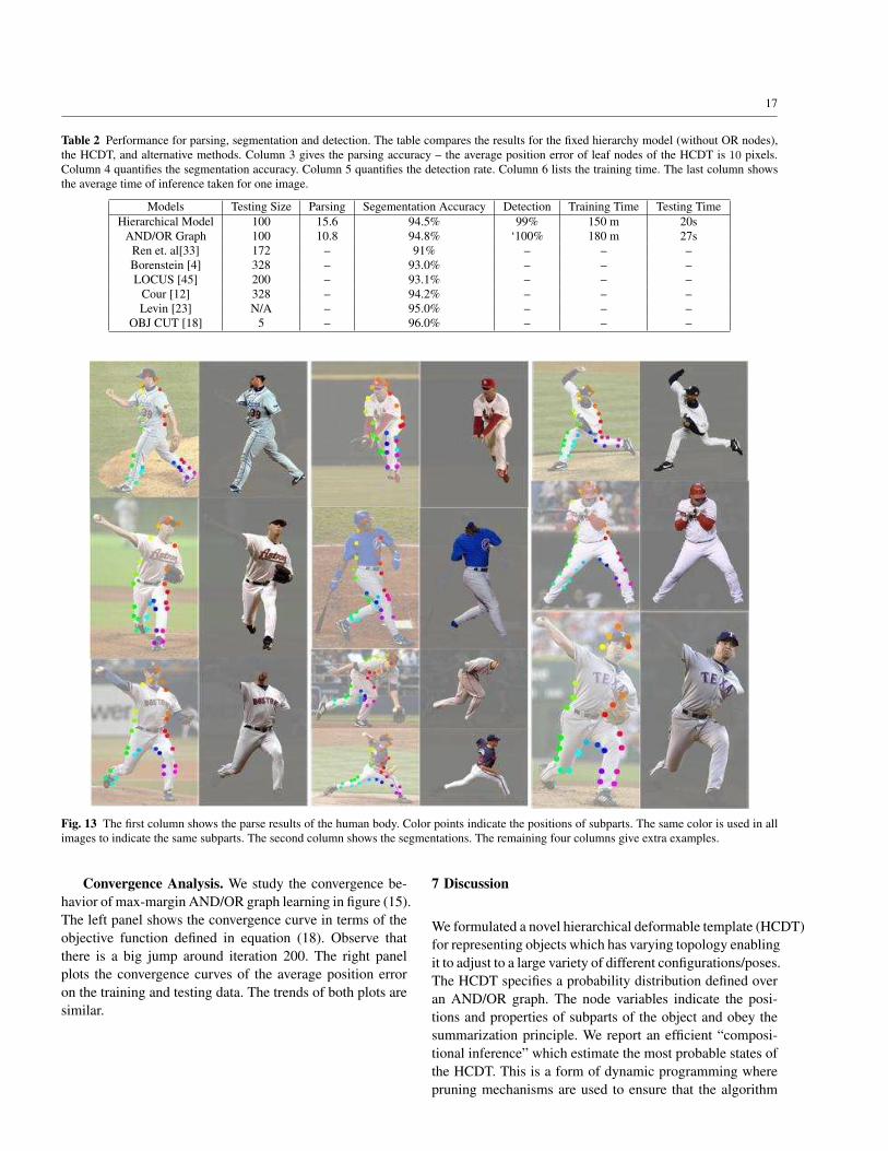
For the baseball dataset Srinivasan and Shi [38] onlyused 5 joint nodes (head-torso, torso-left thigh, torso-rightthigh, left thigh-left lower leg, right thigh-right lower leg).For HCDTs there are 27 nodes on the boundary of eachbaseball player which gives more detailed parsing than al-ternatives [38,26,27]. These 27 points correspond to the 94leaf nodes of the AND/OR graph in figure (2). Each (small-est) part has on average 3.48 (94/27) poses (e.g. orientation).We also asked students to label the parts of the baseballplayers (i.e. to identify different parts of the humans). Forhuman body parsing, we used 48 human baseball images inMori’s dataset [27] as the testing set. The HCDT for humansis able to model 98 poses. In figure (13), observe that thedataset contains a large variety of human poses and the ap-pearance of clothes changes a lot from image to image. Wecreated a training dataset by collecting 156 human baseballimages from the internet and got students to manually labelthe parse tree for each image for training.

Parameter Settings. The HCDT (after training by max-margin) was used to obtain the parse y (i.e. to locate thebody parts). We used max-margin on the training datasetto learn the parameters of the max-margin model. Duringlearning, we set C = 0.1 in equation (18), used the radialbasis function kernel with r = 0.1, set the parameter in theloss function equation (14) to be σ = 12, and set ε = 0.01in figure (7). Our strategy for segmentation, which is in-spired by Grab-Cut [35], is to obtain the parse by the infer-ence algorithm on the HCDT to determine the positions ofthe leaf nodes on the boundary of the object. Then we per-formed postprocessing to give a continuous closed boundaryby graph-cut (using the positions of the leaf nodes to yieldan initial estimate of the feature statistics).

The Parsing Criterion. We used the average positionerror [38] as a criterion to measure the quality of the pars-ing. The position error is defined to be the distance (in pix-els) between the positions of groundtruth and the parsing

14

result (leaf nodes). The smaller the position error, the betterthe quality of the parsing. For horses, there are between 24and 36 leaf nodes which appear on the boundary of a horse.For the baseball player experiments, Srinivasan and Shi [38]only used 5 joint nodes (head-torso, torso-left thigh, torso-right thigh, left thigh-left lower leg, right thigh-right lowerleg) per image. For HCDTs, there are 27 nodes along theboundary of human body which gives more detailed pars-ing.

The Segmentation Criterion Two evaluation criteria areused to measure the performances of segmentation. We usesegmentation accuracy to quantify the proportion of the cor-rect pixel labels (object or non-object). For the baseball playerexperiments, we use the segmentation measure, ‘overlap score’,which is defined by area(P∩G)

area(P∪G) , where P is the area whichthe algorithm outputs as the segmentation and G is the areaof ground-truth. The larger the overlap score, the better thesegmentation.

The Criterion for Weak-Detection We also evaluatedthe performance of HCDTs for the weak-detection task (wherethe object is known to be in the image but its location is un-known). Our criterion judges detection to be successful if thearea of the intersection of the detected object region and thetrue object region is greater than half the area of the unionof these two regions.

6.2 Performance of HCDT’s on the Horse dataset

Results. In table (2) we compare the performances of anHCDT with 40 configurations/topologies against a simplehierarchical model with a fixed topology (i.e. we fix thestates of the OR nodes). The topology of this fixed hierar-chical model (the first one in the top node in figure (3) waschosen to be the topology that most frequently occurred (af-ter doing inference with the HCDT with variable topology).The evaluations are performed on the same 100 test images.To quantify the significance of the improvement made by theHCDT (i.e. the AND/OR representation) we plot the 100paired comparisons in figures (10,11). The p-value for thet-test on parsing is less than 10−5 while the p-value for seg-mentation is 0.03. These tests show that the improvementmade by adding OR nodes is statistically significant for pars-ing (alignment of object parts), but less so for segmentation.

For all experiments we used a computer with 4 GB mem-ory and 2.4 GHz CPU. Learning took 150 minutes for themodel with fixed hierarchy and 180 minutes for the full HCDT.The inference time per image was 20 seconds for the fixedhierarchy model and 27 second for the full HCDT.

Our results show that the HCDT outperforms the fixedhierarchy model for all tasks (i.e. parsing, detection and seg-mentation) with only 30% more computational cost. In fig-ure (12), we compare the parse and segmentation results ob-tained by the fixed hierarchical model and the HCDT. The

0.0

5.0

10.0

15.0

20.0

25.0

30.0

35.0

40.0

45.0

50.0

1 5 9 13 17 21 25 29 33 37 41 45 49 53 57 61 65 69 73 77 81 85 89 93 97

Av

era

ge

po

sit

ion

err

or

# of images

Hierarchical Model And Or Graph

Fig. 10 We compare the parsing performance of hierarchical modeland AND/OR graph on 100 test images.

80.0

82.0

84.0

86.0

88.0

90.0

92.0

94.0

96.0

98.0

100.0

1 5 9

13

17

21

25

29

33

37

41

45

49

53

57

61

65

69

73

77

81

85

89

93

97

Se

ge

me

nta

tio

n A

ccu

racy

# of images

Hierarchical Model And Or Graph

Fig. 11 We compare the segmentation performance of hierarchicalmodel and AND/OR graph on 100 test images.

states of the leaf nodes of parse tree give the estimated po-sitions of the points along the boundary and are illustratedby colored dots (the same colors for corresponding subpartsin different images). Observe that both models (i.e. fixed hi-erarchy and HCDT) are able to deal with large shape defor-mation and appearance variations (after training with maxmargin), see the top four examples, despite cluttered back-ground and varied texture on the horses. But the HCDT ismuch better at locating subparts, such as the legs and thehead, than the fixed hierarchy model which is only able todetect locate the torso reliably. This is illustrated by the lastfour examples in figure (12) where the legs and heads ap-pear in different poses. The fixed hierarchy model succeedsat performing segmentation reasonably well even though itsparsing results are not very good (mainly because of the ef-fectiveness of grab cut). This observation is consistent withthe quantitative comparisons in table (2). But the last exam-ple shows a case where incorrect parsing – the fixed hierar-chy model locates the head in the wrong position – can resultin poor segmentation. In summary, the HCDT performs wellfor both parsing and segmentation in these experiments.

Comparisons. In table (2), we compare the segmenta-tion performance of our approach with other successful meth-ods. Note that the object cut method [18] was reported ononly 5 images. Levin and Weiss [23] make the assumptionthat the position of the object is given (other methods do

15

Fig. 12 This figure is best viewed in color. Columns (a) to (d) show the parsing and segmentation results obtained by the fixed hierarchy modeland the HCDT respectively. The colored dots show the positions of the leaf nodes of the object.

16

Table 3 Empirical Complexity Analysis. This table shows the num-bers of proposals and the time costs at different levels of the hierarchy(“clusters” means the number of proposals accepted after surround sup-pression). ’Aspects’ is the average number of grandchildren nodes foreach level, see text for details.

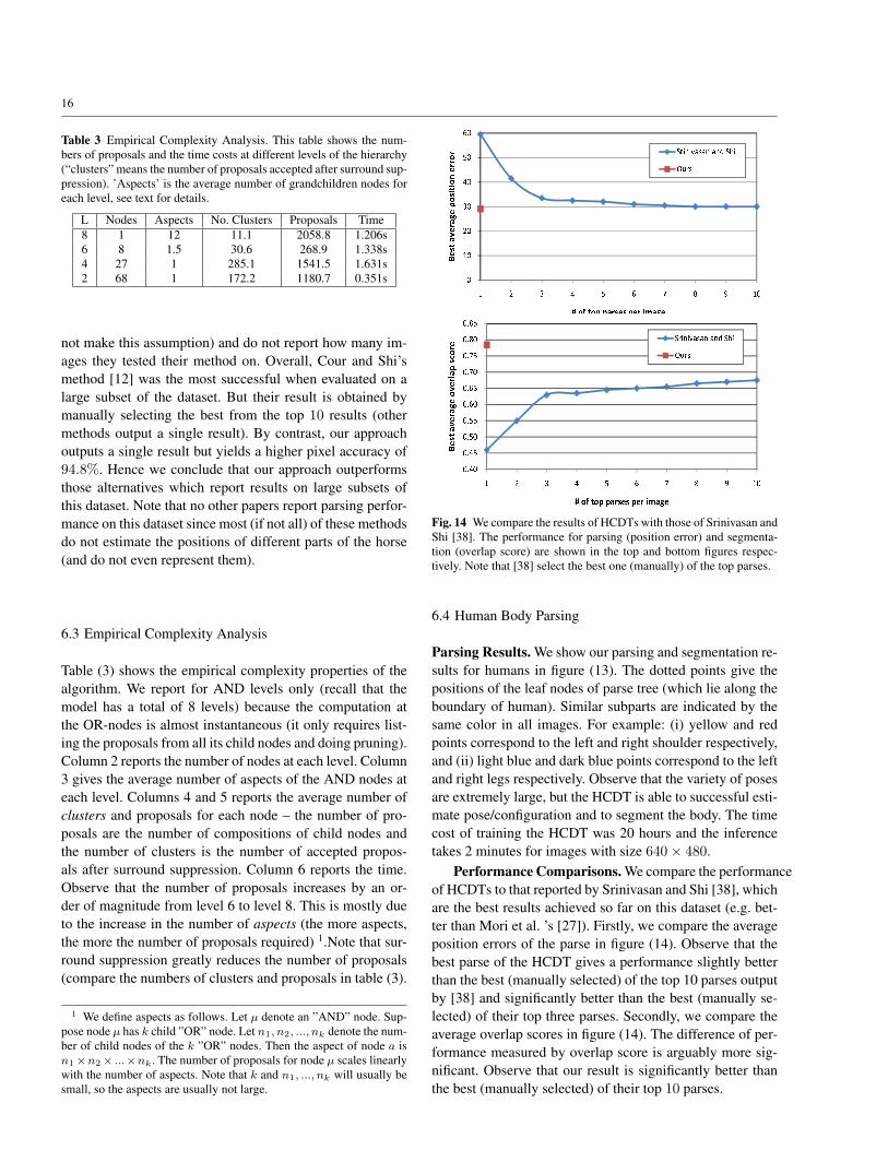
L Nodes Aspects No. Clusters Proposals Time8 1 12 11.1 2058.8 1.206s6 8 1.5 30.6 268.9 1.338s4 27 1 285.1 1541.5 1.631s2 68 1 172.2 1180.7 0.351s

not make this assumption) and do not report how many im-ages they tested their method on. Overall, Cour and Shi’smethod [12] was the most successful when evaluated on alarge subset of the dataset. But their result is obtained bymanually selecting the best from the top 10 results (othermethods output a single result). By contrast, our approachoutputs a single result but yields a higher pixel accuracy of94.8%. Hence we conclude that our approach outperformsthose alternatives which report results on large subsets ofthis dataset. Note that no other papers report parsing perfor-mance on this dataset since most (if not all) of these methodsdo not estimate the positions of different parts of the horse(and do not even represent them).

6.3 Empirical Complexity Analysis

Table (3) shows the empirical complexity properties of thealgorithm. We report for AND levels only (recall that themodel has a total of 8 levels) because the computation atthe OR-nodes is almost instantaneous (it only requires list-ing the proposals from all its child nodes and doing pruning).Column 2 reports the number of nodes at each level. Column3 gives the average number of aspects of the AND nodes ateach level. Columns 4 and 5 reports the average number ofclusters and proposals for each node – the number of pro-posals are the number of compositions of child nodes andthe number of clusters is the number of accepted propos-als after surround suppression. Column 6 reports the time.Observe that the number of proposals increases by an or-der of magnitude from level 6 to level 8. This is mostly dueto the increase in the number of aspects (the more aspects,the more the number of proposals required) 1.Note that sur-round suppression greatly reduces the number of proposals(compare the numbers of clusters and proposals in table (3).

1 We define aspects as follows. Let µ denote an ”AND” node. Sup-pose node µ has k child ”OR” node. Let n1, n2, ..., nk denote the num-ber of child nodes of the k ”OR” nodes. Then the aspect of node a isn1×n2× ...×nk. The number of proposals for node µ scales linearlywith the number of aspects. Note that k and n1, ..., nk will usually besmall, so the aspects are usually not large.

�������������

� � � � � � � � �� �� ����������� � �������

� �� ��� ������ ��� � �!�"#$%$&'('% '%) "*$+,#(

����������������������������������������� � � � � � � ��� � � ������������ �� ���� � �� ��� ������ ��� !�"�

#$%&%'()(& (&* #+%,-$)Fig. 14 We compare the results of HCDTs with those of Srinivasan andShi [38]. The performance for parsing (position error) and segmenta-tion (overlap score) are shown in the top and bottom figures respec-tively. Note that [38] select the best one (manually) of the top parses.

6.4 Human Body Parsing

Parsing Results. We show our parsing and segmentation re-sults for humans in figure (13). The dotted points give thepositions of the leaf nodes of parse tree (which lie along theboundary of human). Similar subparts are indicated by thesame color in all images. For example: (i) yellow and redpoints correspond to the left and right shoulder respectively,and (ii) light blue and dark blue points correspond to the leftand right legs respectively. Observe that the variety of posesare extremely large, but the HCDT is able to successful esti-mate pose/configuration and to segment the body. The timecost of training the HCDT was 20 hours and the inferencetakes 2 minutes for images with size 640× 480.

Performance Comparisons. We compare the performanceof HCDTs to that reported by Srinivasan and Shi [38], whichare the best results achieved so far on this dataset (e.g. bet-ter than Mori et al. ’s [27]). Firstly, we compare the averageposition errors of the parse in figure (14). Observe that thebest parse of the HCDT gives a performance slightly betterthan the best (manually selected) of the top 10 parses outputby [38] and significantly better than the best (manually se-lected) of their top three parses. Secondly, we compare theaverage overlap scores in figure (14). The difference of per-formance measured by overlap score is arguably more sig-nificant. Observe that our result is significantly better thanthe best (manually selected) of their top 10 parses.

17

Table 2 Performance for parsing, segmentation and detection. The table compares the results for the fixed hierarchy model (without OR nodes),the HCDT, and alternative methods. Column 3 gives the parsing accuracy – the average position error of leaf nodes of the HCDT is 10 pixels.Column 4 quantifies the segmentation accuracy. Column 5 quantifies the detection rate. Column 6 lists the training time. The last column showsthe average time of inference taken for one image.

Models Testing Size Parsing Segementation Accuracy Detection Training Time Testing TimeHierarchical Model 100 15.6 94.5% 99% 150 m 20s

AND/OR Graph 100 10.8 94.8% ‘100% 180 m 27sRen et. al[33] 172 – 91% – – –Borenstein [4] 328 – 93.0% – – –LOCUS [45] 200 – 93.1% – – –

Cour [12] 328 – 94.2% – – –Levin [23] N/A – 95.0% – – –

OBJ CUT [18] 5 – 96.0% – – –

Fig. 13 The first column shows the parse results of the human body. Color points indicate the positions of subparts. The same color is used in allimages to indicate the same subparts. The second column shows the segmentations. The remaining four columns give extra examples.

Convergence Analysis. We study the convergence be-havior of max-margin AND/OR graph learning in figure (15).The left panel shows the convergence curve in terms of theobjective function defined in equation (18). Observe thatthere is a big jump around iteration 200. The right panelplots the convergence curves of the average position erroron the training and testing data. The trends of both plots aresimilar.

7 Discussion

We formulated a novel hierarchical deformable template (HCDT)for representing objects which has varying topology enablingit to adjust to a large variety of different configurations/poses.The HCDT specifies a probability distribution defined overan AND/OR graph. The node variables indicate the posi-tions and properties of subparts of the object and obey thesummarization principle. We report an efficient “composi-tional inference” which estimate the most probable states ofthe HCDT. This is a form of dynamic programming wherepruning mechanisms are used to ensure that the algorithm

18 ����������������������� �� � ������������������� � � ��� ��� ��� ��� ��� ��� ��� ��� ��� ���������������������

������� ��� ��� ��� ��� ��� ��� ��� ��� �� ���� �� ���� ��� �� ���� �� ���� ���������

!"#$ %"$!&'() %"$Fig. 15 Convergence Analysis. We study the behavior of max margintraining. The first panel shows the convergence curve of the objectivefunction defined in equation (18). The second panel shows the convergecurves of the average position error evaluated on training and testingset.

is fast when evaluated on two public datasets. The structureof the AND/OR graph is specified by hand but the parame-ters are learnt in a globally optimal way by extending max-margin structure learning technique developed in machinelearning. Advantages of our approach include (i) the abil-ity to model the enormous number of poses/configurationsthat occur for articulated objects such as humans and horses,(ii) the discriminative power provided by max-margin learn-ing (by contrast to MLE), and (iii) the use of the kerneltrick to make use of high-dimensional features. We gave de-tailed experiments on the Weizmann horse and human base-ball datasets, showing improvements over the state-of-the-art methods. We are currently working on improving theinference speed of our algorithm by using a cascade strat-egy. We are also extending the model to represent humansin more details.

Acknowledgements

We gratefully acknowledge support from the National Sci-ence Foundation with NSF grant number 0413214, IIS-0917141,and from the W.M. Keck Foundation.

References

1. Y. Altun, I. Tsochantaridis, and T. Hofmann, “Hidden markov sup-port vector machines,” in ICML, 2003, pp. 3–10.

2. S. Belongie, J. Malik, and J. Puzicha, “Shape matching and objectrecognition using shape contexts,” IEEE Trans. Pattern Anal. Mach.Intell., vol. 24, no. 4, pp. 509–522, 2002.

3. E. Borenstein and S. Ullman, “Class-specific, top-down segmenta-tion,” in ECCV (2), 2002, pp. 109–124.

4. E. Borenstein and J. Malik, “Shape guided object segmentation,” inCVPR (1), 2006, pp. 969–976.

5. X. Chen and A. Yuille, “A time-efficient cascade for real-time ob-ject detection:. with applications for the visually impaired,” in CVPR,2005.

6. H. Chen, Z. Xu, Z. Liu, and S. C. Zhu, “Composite templates forcloth modeling and sketching,” in CVPR (1), 2006, pp. 943–950.

7. Y. Chen, L. Zhu, C. Lin, A. L. Yuille, and H. Zhang, “Rapid infer-ence on a novel and/or graph for object detection, segmentation andparsing,” in NIPS, 2007.

8. H. Chui and A. Rangarajan, “A new algorithm for non-rigid pointmatching,” in CVPR, 2000, pp. 2044–2051.

9. J.M. Coughlan, A. L. Yuille, C. English and D. Snow, “ EfficientOptimization of a Deformable Template Using Dynamic Program-ming,” in CVPR 1998.

10. J.M. Coughlan, A. L. Yuille, C. English and D. Snow,“ EfficientDeformable Template Detection and Localization without User Ini-tialization,” Computer Vision and Image Understanding 78(3): 303-319. 2000.

11. J. M. Coughlan and S. J. Ferreira, “Finding deformable shapesusing loopy belief propagation,” in ECCV (3), 2002, pp. 453–468.

12. T. Cour and J. Shi, “Recognizing objects by piecing together thesegmentation puzzle,” in CVPR, 2007.

13. K. Crammer and Y. Singer, “On the algorithmic implementationof multiclass kernel-based vector machines,” Journal of MachineLearning Research, vol. 2, pp. 265–292, 2001.

14. N. Cristianini and J. Shawe-Taylor, An introduction to supportVector Machines: and other kernel-based learning methods. NewYork, NY, USA: Cambridge University Press, 2000.

15. R. Dechter and R. Mateescu, “And/or search spaces for graphicalmodels,” Artif. Intell., vol. 171, no. 2-3, pp. 73–106, 2007.

16. P. Felzenszwalb and D. McAllester and D. Ramanan,“ A Discrim-inatively Trained, Multiscale, Deformable Part Model” in Proceed-ings of the IEEE CVPR 2008.

17. Y. Jin and S. Geman, “Context and hierarchy in a probabilisticimage model,” in CVPR (2), 2006, pp. 2145–2152.

18. M. P. Kumar, P. H. S. Torr, and A. Zisserman, “Obj cut,” in CVPR(1), 2005, pp. 18–25.

19. J. D. Lafferty, A. McCallum, and F. C. N. Pereira, “Conditionalrandom fields: Probabilistic models for segmenting and labeling se-quence data,” in ICML, 2001, pp. 282–289.

20. S.L. Lauritzen, and D.J. Spiegelhalter. ”Local Computations withProbabilities on Graphical Structures and their Application to ExpertSystems”. Journal of the Royal Statistical Society. Series B. 50 (2):157224. 1988.

21. M. W. Lee and I. Cohen, “Proposal maps driven mcmc for esti-mating human body pose in static images,” in CVPR (2), 2004, pp.334–341.

22. B. Leibe, A. Leonardis, and B. Schiele, “Combined object cat-egorization and segmentation with an implicit shape model,” inECCV’04 Workshop on Statistical Learning in Computer Vision,Prague, Czech Republic, May 2004, pp. 17–32.

23. A. Levin and Y. Weiss, “Learning to combine bottom-up and top-down segmentation,” in ECCV (4), 2006, pp. 581–594.

24. C. Manning and H. Schuetze, Foundations of statistical naturallanguage processing. Cambridge, Mass, USA: MIT Press, 1999.

25. M. Meila and M. I. Jordan, “Learning with mixtures of trees,”Journal of Machine Learning Research, vol. 1, pp. 1–48, 2000.

19

26. G. Mori, X. Ren, A. A. Efros, and J. Malik, “Recovering humanbody configurations: Combining segmentation and recognition,” inCVPR (2), 2004, pp. 326–333.

27. G. Mori, “Guiding model search using segmentation,” in ICCV,2005, pp.1417–1423.

28. M. Oren, C. Papageorgiou, P. Sinha , E. Osuna and T. Poggio,“Pedestrian detection using wavelet templates,” In Proc. ComputerVision and Pattern Recognition, pages 193–199, Puerto Rico, June16–20 1997.

29. E. Osuna, R. Freund, and F. Girosi, “Training support vector ma-chines: an application to face detection,” in CVPR, 1997, pp. 130–136.

30. J. C. Platt, “Using analytic qp and sparseness to speed training ofsupport vector machines,” in NIPS, 1998, pp. 557–563.

31. D. Ramanan, “Learning to parse images of articulated bodies,” inNIPS, 2006, pp. 1129–1136.

32. X. Ren, A. C. Berg, and J. Malik, “Recovering human body con-figurations using pairwise constraints between parts,” in ICCV, 2005,pp. 824–831.

33. X. Ren, C. Fowlkes, and J. Malik, “Cue integration for fig-ure/ground labeling,” in NIPS, 2005.

34. R. Ronfard, C. Schmid, and B. Triggs, “Learning to parse picturesof people,” in ECCV (4), 2002, pp. 700–714.

35. C. Rother, V. Kolmogorov, and A. Blake, ““grabcut”: interac-tive foreground extraction using iterated graph cuts,” ACM Trans.Graph., vol. 23, no. 3, pp. 309–314, 2004.

36. L. Sigal and M. J. Black, “Measure locally, reason globally:Occlusion-sensitive articulated pose estimation,” in CVPR (2), 2006,pp. 2041–2048.

37. P. Srinivasan and J. Shi, “Bottom-up recognition and parsing ofthe human body,” in EMMCVPR, 2007, pp. 153–168.

38. P. Srinivasan and J. Shi, “Bottom-up recognition and parsing ofthe human body,” in CVPR, 2007.

39. B. Taskar, C. Guestrin, and D. Koller, “Max-margin markov net-works,” in NIPS, 2003.

40. B. Taskar, D. Klein, M. Collins, D. Koller, and C. Manning, “Max-margin parsing,” in EMNLP, 2004.

41. I. Tsochantaridis, T. Hofmann, T. Joachims, and Y. Altun, “Sup-port vector machine learning for interdependent and structured out-put spaces,” in ICML, 2004.

42. V. N. Vapnik, The nature of statistical learning theory. New York,NY, USA: Springer-Verlag New York, Inc., 1995.

43. P. A. Viola and M. J. Jones, “Robust real-time face detection,”International Journal of Computer Vision, vol. 57, no. 2, pp. 137–154, 2004.

44. P. Viola, J. C. Platt, C. Zhang, “Multiple Instance Boosting forObject Detection,”in NIPS 2005.

45. J. M. Winn and N. Jojic, “Locus: Learning object classes withunsupervised segmentation,” in ICCV, 2005, pp. 756–763.

46. J. Zhang, J. Luo, R. T. Collins, and Y. Liu, “Body localization instill images using hierarchical models and hybrid search,” in CVPR(2), 2006, pp. 1536–1543.

47. L. Zhu, Y. Chen, and A. L. Yuille, “Unsupervised learning of aprobabilistic grammar for object detection and parsing,” in NIPS,2006, pp. 1617–1624.

48. L. Zhu and A. L. Yuille, “A Hierarchical Compositional Systemfor Rapid Object Detection,” in NIPS, 2005.

49. L. Zhu, Y. Chen and A. Yuille, “ Unsupervised Learning of Prob-abilistic Grammar-Markov Models for Object Categories,” IEEETrans. Pattern Anal. Mach. Intell. 2009.

50. L. Zhu, C. Lin, H. Huang, Y. Chen and A. Yuille, “ UnsupervisedStructure Learning: Hierarchical Recursive Composition, SuspiciousCoincidence and Competitive Exclusion,” in ECCV 2008.

51. L. Zhu, Y. Chen, Y. Lu, C. Lin and A. Yuille, “Max MarginAND/OR Graph Learning for Parsing the Human Body,” in CVPR2008.

52. S. Zhu and D. Mumford, “A stochastic grammar of images,” vol. 2,no. 4, pp. 259–362, 2006.