max dama automated trading
TRANSCRIPT
Max Dama onAutomated TradingJune 2008 - May 2011
Contents
1 Introduction 3
2 Industry 42.1 History . . . . . . . . . . . . . . . . . . 42.2 Overview . . . . . . . . . . . . . . . . . 52.3 Buy Side . . . . . . . . . . . . . . . . . . 52.4 Companies . . . . . . . . . . . . . . . . 72.5 Sell Side . . . . . . . . . . . . . . . . . . 8
3 Brainteasers 83.1 Market Making and Betting . . . . . . . 93.2 Probability . . . . . . . . . . . . . . . . 93.3 Retention of Coursework . . . . . . . . . 103.4 Mental Math . . . . . . . . . . . . . . . 103.5 Pattern Finding . . . . . . . . . . . . . . 113.6 Math and Logic . . . . . . . . . . . . . . 12
4 Alpha 134.1 Reuter’s Carrier Pigeons . . . . . . . . . 154.2 Traffic Analysis . . . . . . . . . . . . . . 154.3 Dispersion . . . . . . . . . . . . . . . . . 164.4 StarMine . . . . . . . . . . . . . . . . . 164.5 First Day of the Month . . . . . . . . . 174.6 Stock Market Wizards . . . . . . . . . . 174.7 Weighted Midpoint . . . . . . . . . . . . 174.8 Toolbox . . . . . . . . . . . . . . . . . . 174.9 Machine Learning . . . . . . . . . . . . . 214.10 Checklist . . . . . . . . . . . . . . . . . 22
5 Simulation 235.1 Data . . . . . . . . . . . . . . . . . . . . 235.2 Simulators . . . . . . . . . . . . . . . . . 245.3 Pitfalls . . . . . . . . . . . . . . . . . . . 255.4 Optimization . . . . . . . . . . . . . . . 265.5 Extra: Michael Dubno . . . . . . . . . . 28
6 Risk 286.1 Single Strategy Allocation . . . . . . . . 296.2 Multiple Strategies . . . . . . . . . . . . 316.3 Porfolio Allocation Summary . . . . . . 346.4 Extra: Empirical Kelly Code . . . . . . 346.5 Extra: Kelly ≈ Markowitz . . . . . . . . 37
7 Execution 387.1 Liquidity Impact . . . . . . . . . . . . . 397.2 Slicing Up Orders . . . . . . . . . . . . . 397.3 Alpha Loss . . . . . . . . . . . . . . . . 407.4 Execution Shortfall . . . . . . . . . . . . 417.5 Capacity . . . . . . . . . . . . . . . . . . 417.6 Practical Transaction Costs . . . . . . . 427.7 Extra: Measuring Impact . . . . . . . . 43
8 Programming 478.1 Design Patterns . . . . . . . . . . . . . . 478.2 Common Specialized Patterns . . . . . . 498.3 APIs . . . . . . . . . . . . . . . . . . . . 498.4 Programming Language . . . . . . . . . 538.5 OS and Hardware Platform . . . . . . . 54
9 Fix-it Game 55
10 Pit Trading Game 56
11 Recommended Media 58
1
1 Introduction
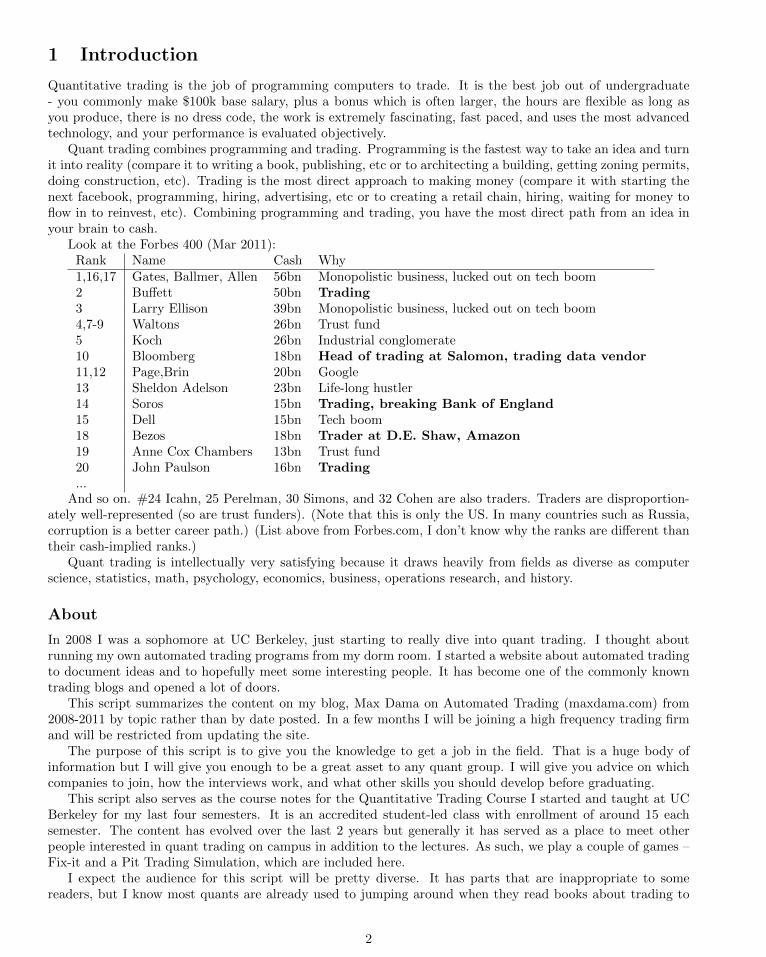
Quantitative trading is the job of programming computers to trade. It is the best job out of undergraduate- you commonly make $100k base salary, plus a bonus which is often larger, the hours are flexible as long asyou produce, there is no dress code, the work is extremely fascinating, fast paced, and uses the most advancedtechnology, and your performance is evaluated objectively.
Quant trading combines programming and trading. Programming is the fastest way to take an idea and turnit into reality (compare it to writing a book, publishing, etc or to architecting a building, getting zoning permits,doing construction, etc). Trading is the most direct approach to making money (compare it with starting thenext facebook, programming, hiring, advertising, etc or to creating a retail chain, hiring, waiting for money toflow in to reinvest, etc). Combining programming and trading, you have the most direct path from an idea inyour brain to cash.
Look at the Forbes 400 (Mar 2011):Rank Name Cash Why1,16,17 Gates, Ballmer, Allen 56bn Monopolistic business, lucked out on tech boom2 Buffett 50bn Trading3 Larry Ellison 39bn Monopolistic business, lucked out on tech boom4,7-9 Waltons 26bn Trust fund5 Koch 26bn Industrial conglomerate10 Bloomberg 18bn Head of trading at Salomon, trading data vendor11,12 Page,Brin 20bn Google13 Sheldon Adelson 23bn Life-long hustler14 Soros 15bn Trading, breaking Bank of England15 Dell 15bn Tech boom18 Bezos 18bn Trader at D.E. Shaw, Amazon19 Anne Cox Chambers 13bn Trust fund20 John Paulson 16bn Trading...
And so on. #24 Icahn, 25 Perelman, 30 Simons, and 32 Cohen are also traders. Traders are disproportion-ately well-represented (so are trust funders). (Note that this is only the US. In many countries such as Russia,corruption is a better career path.) (List above from Forbes.com, I don’t know why the ranks are different thantheir cash-implied ranks.)
Quant trading is intellectually very satisfying because it draws heavily from fields as diverse as computerscience, statistics, math, psychology, economics, business, operations research, and history.
About
In 2008 I was a sophomore at UC Berkeley, just starting to really dive into quant trading. I thought aboutrunning my own automated trading programs from my dorm room. I started a website about automated tradingto document ideas and to hopefully meet some interesting people. It has become one of the commonly knowntrading blogs and opened a lot of doors.
This script summarizes the content on my blog, Max Dama on Automated Trading (maxdama.com) from2008-2011 by topic rather than by date posted. In a few months I will be joining a high frequency trading firmand will be restricted from updating the site.
The purpose of this script is to give you the knowledge to get a job in the field. That is a huge body ofinformation but I will give you enough to be a great asset to any quant group. I will give you advice on whichcompanies to join, how the interviews work, and what other skills you should develop before graduating.
This script also serves as the course notes for the Quantitative Trading Course I started and taught at UCBerkeley for my last four semesters. It is an accredited student-led class with enrollment of around 15 eachsemester. The content has evolved over the last 2 years but generally it has served as a place to meet otherpeople interested in quant trading on campus in addition to the lectures. As such, we play a couple of games –Fix-it and a Pit Trading Simulation, which are included here.
I expect the audience for this script will be pretty diverse. It has parts that are inappropriate to somereaders, but I know most quants are already used to jumping around when they read books about trading to
2

try to extract all the useful bits, and sift through the mumbo jumbo and filler. I have attempted to omit all thefiller and of course mumbo jumbo. While this is relative, most books seem to inanely target a certain page count(150+) in order to be seen as a more legitimate book. Besides this sentence, I try to ignore this compulsion.This book has a lower price than any other book on quant trading because I have no editor. It has fewer pagesbecause the pages are much bigger to accommodate code more clearly. Please take it for what it is.
The best way to read this script is to jump to sections you are interested in. However, read the Risk andExecution sections sequentially because they follow a logical flow. If you are completely new to quant trading,e.g. you are in college, read each section in order starting from “Industry”.
Please email me at [email protected] if you have comments.
2 Industry
Work shall set you free
2.1 History
A big purpose of the Quantitative Trading Course’s history lecture is just presenting material that is friendly tothe class asking questions. The content is fictional but draws lots of questions about how markets and differentproducts function. It is many students’ first introduction to how markets work. Sketches on the whiteboard area big part of the lecture but are not included here.
Wall Street seems pretty complicated today, but if you look at how trading started, it’s much easier tounderstand.
Arabia 0 B.C.
• Venue: Bazaar
• Participants: Traders, Merchants, Villagers
• Reasons: hedgers, informed traders, liquidity seekers, position traders
• Traders can become market makers by setting up a tent
• Queues form outside of market maker’s tents
• Market is based on the Bazaar’s schedule and the merchant’s travel plans
Wall Street 1880
• Venue: Banks’ Telephones
• Participants: Bankers acting as market makers and as salesmen
• Reasons: Ripping off clients
• Electronic communication
• Trading fees and bid/ask spreads
• Goods, money, and trading separate
Wall Street 1950
• Venue: Big Board
• Participants: Pit traders, specialists
• Reasons: investment, speculation, excitement
3
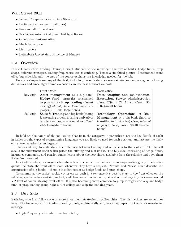
Wall Street 2011
• Venue: Computer Science Data Structure
• Participants: Traders (in all roles)
• Reasons: all of the above
• Trades are automatically matched by software
• Guarantees best execution
• Much faster pace
• Limit orders
• Heisenberg Uncertainty Principle of Finance
2.2 Overview
In the Quantitative Trading Course, I orient students to the industry. The mix of banks, hedge funds, propshops, different strategies, trading frequencies, etc, is confusing. This is a simplified picture. I recommend frontoffice buy side jobs and the rest of the course explains the knowledge needed for the job.
Here is a simple taxonomy of the field, including the sell side since some strategies can be augmented usingderivatives and since algorithmic execution can decrease transaction costs:
Front Office Back OfficeBuy Side Asset management at a big bank.
Hedge fund (strategies constrainedto prospectus) Prop trading (fastestmoving) Matlab, Java, Functional Lan-guages. 70-100k+large bonus
Data scraping and maintenance,Execution, Server administrationBash, SQL, SVN, Linux, C++. 90-100k+small bonus
Sell Side Sales & Trading at a big bank (taking& executing orders, creating derivativesby client reques, execution algos) Excel.70-80k+medium bonus
Technology, Operations, or RiskManagement at a big bank (hard totransition to front office) C++, internallanguage, hacky code. 90-100k+smallbonus
In bold are the names of the job listings that fit in the category; in parentheses are the key details of each;in italics are the types of programming languages you are likely to need for each position; and last are the likelyentry level salaries for undergrads.
The easiest way to understand the difference between the buy and sell side is to think of an IPO. The sellside is the investment bank which prices the offering and markets it. The buy side, consisting of hedge funds,insurance companies, and pension funds, learns about the new shares available from the sell side and buys themif they’re interested.
Front office refers to someone who interacts with clients or works in a revenue-generating group. Back officequants facilitate the front office team whenever they have a request. “Front” and “back” office describe theorganization of big banks – there is less distinction at hedge funds and prop shops.
To summarize the easiest cookie-cutter career path in a sentence, it’s best to start in the front office on thesell side, specialize in a certain product, and then transition to the buy side about halfway in your career aroundVP level of course staying front office. It’s also becoming more common to jump straight into a quant hedgefund or prop trading group right out of college and skip the banking years.
2.3 Buy Side
Each buy side firm follows one or more investment strategies or philosophies. The distinctions are sometimeshazy. The frequency a firm trades (monthly, daily, millisecondly, etc) has a big impact on the firm’s investmentstrategy.
• High Frequency - intraday: hardware is key
4

Market Making Get inside the bid-ask spread and buy low, sell high
Arbitrage Take advantage of things trading at different prices on different exchanges or through differentderivatives
Momentum If it’s going up, it’s going to go up more: filters are key
Mean Reversion If it’s going up, it’s going to go down: filters are key
• Low Frequency - monthly holding period: bigger better models win
Relative Value model stock-vs-stock by management quality, accounting criteria (often normalized bysector), analyst estimates, news, etc
Tactical Asset Allocation model sector-vs-currency-vs-commodities by macroeconomic trends, com-modity prices, FX rates: the key word is factors - research them and add them to the company’smodel
• Specialty
Emerging market for example the India Fund
Behavioral model human-vs-self
News Based text mining, web scraping, NLP
5

2.4 Companies
College grads should apply to every single company onthis list if possible. The best way to get a job is not tocarefully court a specific firm, but to apply to as manyas possible.
Internship
• Jane Street
• SIG
• IMC
• DE Shaw
• Jump
Full Time
• Renaissance
• Getco
• Jane Street
• Allston
• IMC
• Chopper
• Hudson River Trading
• Optiver
• CTC
• Fox River Partners
• Sun Trading
• Matlock Capital
• Ronin Capital
• Tradelink
• DRW
• Traditum
• Infinium
• Transmarket
• Spot
• Geneva Trading
• Quantres
• Tradebot
• Tradeworx
• Virtu
• Cutler Group
• Two Sigma
• Millennium / World Quant
• SAC
• HBK
• Citadel
• IV Capital
• Tower Research
• Knight
• Blue Crest
• Winton Capital
• GSA Capital
Startups (as of Mar 2011)
• Headlands
• Teza
• Aardvark
• Eladian
• AienTech
• Circulum Vite
6
2.5 Sell Side
In this script I don’t focus on the sell side. However it is usually the first step available to new grads to get intothe industry. Look on any big bank’s (Goldman, MS, UBS, etc) website for positions titled “Sales and Trading”to apply. It’s hard to say which banks are good or bad because it varies desk to desk, product to product.
Derivatives
When most people talk about financial engineering, they are referring to derivatives. Derivatives are not a topicof this script either so I briefly give the main idea of them here and then move on.
Most derivatives are just combinations of swaps and options. You should already be familiar with options.Swaps are basically pieces of paper that entitle the signing parties to get money from each other depending onwhat happens in the future. For example interest rate swaps entitle one party to payments based on the levelof let’s say LIBOR while the other gets fixed payments. Another example are credit default swaps which entitleone party to a lump sum of cash if a company fails to pay interest on a loan (defaults) while the other getsperiodic payments in normal conditions. A final example are equity swaps. A bank will buy a stock you wantto own and then sell you a peice of paper saying you owe them for it. For example, if you are Mark Cuban andyou get $5.7 billion worth of YHOO stock but you are contractually restricted from selling it, you can sell anequity swap on YHOO and completely sidestep the legal restrictions. The bank hedges their risk by selling thestock and you don’t have to worry if there is a tech bubble because you essentially dumped your stock.
In general, derivatives are designed for one or more of the following reasons:
• Avoid or shield taxes
• Decrease capital or margin requirements
• Repackage risk factors (ex. skew swaps)
• Dodge other regulations: short sale restrictions, international investment restrictions, AAA rating require-ments
Algorithmic Execution
The phrase “algorithmic trading” has a different meaning depending on if you are in Chicago or New York. InChicago it will mean using a computer to place trades to try to make a profit. In New York it means to use acomputer to work client orders to try to minimize impact.
Algorithmic execution/trading (in the New York sense) is the automation of the role of the execution trader.We will talk more about algos later in the context of transaction cost minimization. However realize that thisis one popular quant job for college grads.
3 Brainteasers
When you laugh, the world laughs with you. When you cry, you cry alone. –Korean proverb
I never wanted to do brainteasers. I thought I should spend my time learning something useful and not tryto “game” job interviews. Then I talked to a trader at Deutche Bank that hated brainteasers but he told methat he, his boss, and all his co-workers did brainteasers with each other everyday because if DB ever failed orthey somehow found themselves out of a job (even the boss), then they knew they would have to do brainteasersto get another. So I bit the bullet and found out it does not take a genius to be good at brainteasers, just a lotof practice.
In this section are brainteasers I have gotten in interviews with quantitative high frequency trading groups.
7
3.1 Market Making and Betting
• Flip 98 fair coins and 1 HH coin and 1 TT coin. Given that you see an H, what is the probability that itwas the HH coin? Explain in layman’s terms.
• Flip 10000 fair coins. You are offered a 1-1 bet that the sum is less than 5000. You can bet 1, 2, ..., 100dollars. How much will you bet. How much will you bet if someone tells you that the sum of the coins isless than 5100?
• Roll a die repeatedly. Say that you stop when the sum goes above 63. What is the probability that thesecond to last value was X. Make a market on this probability. Ie what is your 90 percent confidenceinterval.
• There are closed envelopes with $2, $4, $8, $16, $32, and $64 lined up in sorted order in front of you.Two envelopes next to each other are picked up and shuffled. One is given to you and one is given to yourfriend. You and you friend then open your own envelopes, look inside, and then decide whether or not tooffer to trade. If you both agree to trade, then you will swap. Assume you open your envelope and see$16. Should you offer to trade?
• Generate N random values from a random variable where the value N comes from some other variable.Make a market on the sum of the values.
• Find the log-utility optimal fraction of your capital to bet on a fair coinflip where you win x on a headsand lose y on tails.
• This question is very hard to explain. It is intended to judge how much of a feel you have for risk in anadversarial setting with various bits of information about how much your counterparty might be trying toscrew you and how much control they have over the game. It goes something like this: The interviewer,who has the mannerisms of an amateur magician, holds up a top hat. He puts five yellow nerf balls in it.Pulls one ball from the hat. It is a yellow nerf ball. Would you bet on the next four balls being yellow?What if I made you pay to play? What if I was your friend? What if your friend put the balls in? Whatif I made you pay more? etc etc...
• Explain how you would handle a trading model with 25 factors differently than one with 100. What youwould ask or do next if the 100 factor model had 25% better performance than the 25 factor model?
• If a stock starts at a price of p and then goes up x% then down x%, is its price greater than, less than, orequal to p?
• You have 100 dollars. You are playing a game where you wager x dollars on a biased coin flip with a 90percent probability of heads. You make 2x if it’s heads and lose the x dollars if it’s tails. How much doyou think you should bet on each flip if you are going to play for 100 flips?
• Make a market on a derivative with a price equal to the number of pothole covers in New York.
3.2 Probability
• What is the pobability of getting exactly 500 heads out of 1000 coin flips? Approximate it to within 5%of the true value without a calculator.
• Play a game like chess or pingpong. You only have two opponents, A and B. A is better than B. Youwill play three games. There are only two orders you can play: ABA and BAB. Which gives you a betterchance of winning?
• Play a 1 vs 1 game. I roll a 6 sided die, if I get a 1 I win, if not you roll. If you get a 6 you win, otherwiseI go again... What are my chances of winning and what are yours?
• Normal 52 card deck. Cards are dealt one-by-one. You get to say when to stop. After you say stopyou win a dollar if the next card is red, lose a dollar if the next is black. Assuming you use the optimalstopping strategy, how much would you be willing to pay to play? Proof?
8

• Assume there is a diagnostic drug for detecting a certain cancer. It is 99% sensitive and 99% specific.0.5% of the population has this cancer. What is the probability that a randomly selected person from thepopulation has this cancer given that you diagnose them using the drug and it comes back positive?
• You have 3 pancakes in a stack. 1 is burned on both sides, 1 burned on 1 side, 1 burned on no sides.What is P(burned on other side — burned on the top)?
• Roll a die until the first 6. What’s the expected number of rolls? What’s the expected number of rollsuntil two sixes in a row? How about a six then a five? Are they different?
• Say you roll a die, and are given an amount in dollar equal to the number on the die. What would youpay to play this game if you played it a many times in a row? Now say that when you roll the die, you’reallowed to either take the money that you’d get with the roll, or roll a second time; if you roll a secondtime, you’re obligated to take the number of dollars that you get with the second roll. Now what is theworth of the game? Same thing as above, except you have an option to play the game a third time.
• Let’s say you’re playing a two-player game where you take turns flipping a coin and whoever flips headsfirst wins. If the winner gets 1 dollar, how much would you pay to go first instead of second?
• Two fair coins are flipped behind a curtain. You are told at least one came up heads. Given thatinformation and nothing else, what is the probability that both landed heads?
• You are trying to determine the price a casino should charge to play a dice game. The player rolls a dieand gets paid the amount on the face, however he can choose to re-roll the dice, giving up the chanceto take the first payout amount before seeing the second result. Similarly he has the same option onthe second roll, but after the second re-roll, he must keep the amount shown the third time. How muchshould the casino charge to break even in expectation on this game assuming the player chooses the beststrategy?
• You have 5 quarters on the table in front of you: four fair (regular two-sided coins) and one double-sided(both sides are heads). You pick one of them up at random, flip it five times, and get heads each time.Given this information, what is the probability that you picked up the double-sided quarter?
3.3 Retention of Coursework
• Analyze the results of a multiple linear regression given a few plots, datapoints, and p-values.
• Explain collinearity
• Assume you have data generated by the process y = Ax + w where w is white noise. What is the leastsquares estimate of x? Give the matrix equation and the intuition behind “least squares”.
• What is the t-value in a linear regression and how is it calculated?
• Derive the maximum likelihood estimate for the mean of a bernoulli random variable given data [on awhiteboard].
• If v is a column vector, then how many non-zero eigenvalues does the matrix aaT have? what are theeigenvalues? What are the corresponding eigenvectors? What are the eigenvectors corresponding to thezero eigen values?
3.4 Mental Math
Answer as quickly as possible.
• 73
• 15% of 165
9
• one million minus 1011
• 54% of 123
• 552
3.5 Pattern Finding
• Find the next number in the sequence (2.1 pts):
1, 3, 7, 12, 18, 26, 35, 45, 56, 69, 83, 98, 114, 131...
Ans: 150
Sol: take first differences twice (second differences) and then notice the pattern:
first diffs: 2, 4, 5, 6, 8, 9, 10, 11, 13, 14, 15, 16, 17
2nd diffs: 2, 1, 1, 2, 1, 1, 1, 2, 1, 1, 1, 1, 2, so the next first diff is 19, so the next number is 150
• Find three whole, positive numbers that have the same answer when multiplied together as when addedtogether (1.0 pt).
Ans: 1, 2, 3
• We put a spore in a test tube. Every hour the spore divides into three parts, each the same size as theoriginal spore. If we put the first spore in the tube at noon and at 6pm the tube is completely full, atwhat time is the tube 1/3 full? (1.8 pts)
Ans: 5pm
• If 75% of all women are tall, 75% of all women are brunette, and 75% of all women are pretty, what is theminimum percentage who are tall, brunette, pretty women? (2.7 pts)
Ans: 25%
Sol: Use geometric probability
• A month begins on a Friday and ends on a Friday, too. What month is it? (1.0 pt)
Ans: February
Sol: February is the only month with a number of days which is divisible by 7 (28 days).
• There is one in a minute, two in a moment, but only one in a million years. What is it? (1.1 pts)
Ans: the letter ‘m’
Sol: ‘m’inute = 1; ‘m’o‘m’ent = 2; ‘m’illion years = 1
• Find the next number in this sequence: (3.2 pts)
1248, 1632, 6412, 8256...
Ans: 5121
Sol: Write down the sequence: 1, 2, 4, 8, 16, 32, 64, 128, 256...
Delete all the spaces: 1248163264128256...
Add spaces back after ever four numbers to get the original sequence.
So extending it we know the next numbers are 512, 1024 ie 5121024 ie 5121, ...
10
3.6 Math and Logic
• A girl is swimming in the middle of a perfectly circular lake. A wolf is running at the edge of the lakewaiting for the girl. The wolf is within a fence surrounding the lake, but it cannot get out of the fence.The girl can climb over the fence. However if the wolf is at the edge of the lake where the girl touches it,then it will eat her. The wolf runs 2 times faster than the girl can swim. Assume the wolf always runstoward the closest point on the edge of the lake to where the girl is inside. Can the girl escape? If so,what path should she swim in?
• The hands on a clock cross each other at midnight. What time do they cross each other next?
• Three people are standing in a circle in a duel. Alan has 100% accuracy, Bob has 66% accuracy, and Carlhas 33%. It is a fight to the death – only one person can walk away. They take turns starting with Carl,then Bob, then Alan, and so on. Assume each person plays rationally to maximize their chance of walkingaway. What is Carl’s action on the first round?
• xxxxx···
= 2. What is x?
• What is
√2 +
√2 +
√2 +
√2 +√
2 + · · ·?
• A line segment is broken into three pieces. What is the probability they form a triangle?
• What is the probability that three points chosen uniformly and independently on a circle fall on a semi-circle?
• We have two concentric circles. A chord of the larger circle is tangent to the smaller circle and has length8. What’s the area of the annulus–the region between the two circles?
• There are a cup of milk and a cup of water. Take one teaspoon of milk, put into the water cup; mix well.Take one teaspoon of the mixture in the water cup and put into the milk cup then mix well. Which ishigher: the percentage of water in the milk cup or the percentage of milk in the water cup ?
• Two trains are 30 miles apart and are on track for a head-on collision – one train is going at 20 milesper hour and the the other is going at 40 miles per hour. If there is a bird flying back and forth betweenthe fronts of the two trains at 10 miles per hour, what is the total distance the bird will travel before thetrains hit?
• A 10-by-10-by-10 cube constructed from 1-by-1-by-1 cubes falls into a bucket of paint. How many littlecubes have at least one face with paint on it?
• Write a function to find the median of a list.
• You have an unsorted array of the numbers 1 to 50 in a random order. Let’s say one of the numbers issomehow missing. Write an efficient algorithm to figure which is missing.
• What is (1 + 1n )n as n→∞?
• The number of lilipads on a pond doubles each minute. If there is 1 lilipad initially at time t = 0, therefore2 at t = 1, 4 at t = 3, 8 at t = 4, etc and the pond is totally covered at time t = 60, then how much ofthe pond’s surface is still visible at time t = 58?
• How can a cheesecake be cut three times to get eight equal slices?
• The airplane passengers problem (can be looked up in the brainteasers forum): say you have 100 passengersboarding a plane with 100 seats. the first person to board is a weird old lady who, instead of going to herown seat, seats in one of the seats uniformly at random (she could pick her own, but she could also picksomeone else’s seat). From then on, when a person boards, they’ll sit in their own seat if it’s available,and if their seat is taken by someone, they’ll pick one of the remaining seats uniformly at random and sitthere. What is the probability that the last person sits in his/her own seat?
11
• A company has a value V which is uniformly distributed between 0 and 1. You are planning to place abid B for the company. If B is smaller than V, then your bid loses and you get nothing; if B is larger thanV, you get to purchase the company at price B, and the company will end up being worth 1.5 * V. Whatprice B should you bid to maximize your profit?
• On a sheet of paper, you have 100 statements written down. the first says, “at most 0 of these 100statements are true.” The second says, “at most 1 of these 100 statements are true.” ... The nth says,“at most (n-1) of these 100 statements are true.” ... the 100th says, “at most 99 of these statements aretrue.” How many of the statements are true?
• You and your spouse host a party with eight other couples. At the beginning of the party, people proceedto shake the hands of those they know. No one shakes their own hand or their spouse’s hand. After thisshaking of hands is done, you take a survey of how many hands each person shook, and it turns out thatexcluding yourself, the numbers of hands shook by everyone else are distinct—that is, no one shook thesame number of hands as anyone else. How many hands did your spouse shake?
• You have two decks of cards: one has 13 reds and 13 blacks, and the other has 26 reds and 26 blacks. Weplay a game in which you select one of the two decks, and pick two cards from it; you win the game ifyou select two black cards. Which deck should you select to maximize your chances of winning? Try todo this problem in your head, without writing any calculations down.
• You have a deck of 52 cards, and you keep taking pairs of cards out of the deck. If a pair of cards are bothred, then you win that pair; if a pair of cards are both black, then I win that pair; if a pair of cards hasone red and one black, then it’s discarded. If, after going through the whole deck, you have more pairsthan I do, then you win 1 dollar, and if I have more pairs than you do, I win 1 dollar. What is the valueof this game in the long run?
4 Alpha
A man always has two reasons for doing anything: a good reason and the real reason. –J.P. Morgan
Alpha is the ability to predict the future. Alpha is defined as the additional return over a naive forecast.Finding alpha is the job of a quant research analyst.
Alpha comes from four sources:
• Information
• Processing
• Modeling
• Speed
Speed is a source of alpha since acting in the future relative to other traders is equivalent to predicting thefuture (think of the uncertainty principle).
A toy example of predicting a person’s weight from height illustrates the first three. The naive predictonis that weight will be equal to the mean weight of the overall population. An improved prediction is weight =mean(weight) + β ∗ height3 where β is the regression coefficient. The informational alpha is the use of height.The preprocessing alpha is cubing height. The modeling alpha is usage of the linear model. Modeling andprocessing are only subtly different in this case.
There are six common trading strategies. These are frameworks for coming up with new models and jargonfor communicating concisely. These are not exhaustive. The pairs of stacked horizontal bars are the bid andoffer. Remember a market order is buying at an offer or selling at a bid and a limit order is selling at an offeror buying at a bid. Imagine a vertical y-axis with price.
12
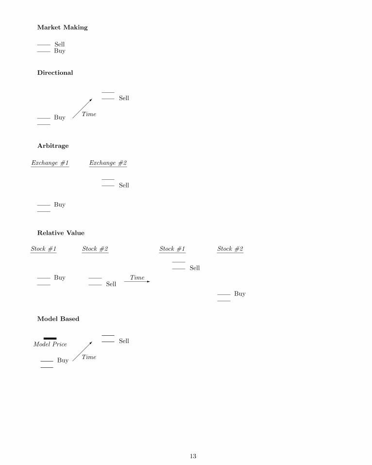
Market Making
SellBuy
Directional
Sell
����
TimeBuy
Arbitrage
Exchange #2
Sell
Exchange #1
Buy
Relative Value
Stock #2
Sell
Stock #1
Buy -Time
Stock #1
Sell
Stock #2
Buy
Model Based
Model Price Sell
����
TimeBuy
13
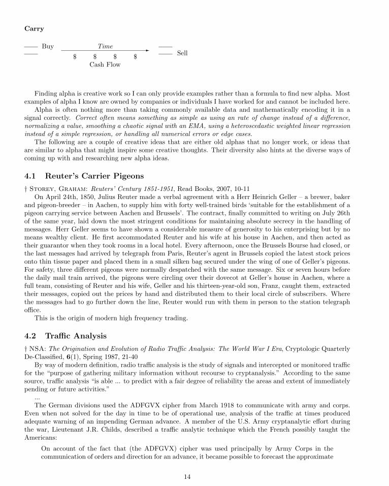
Carry
Buy -TimeSell
$ $ $ $Cash Flow
Finding alpha is creative work so I can only provide examples rather than a formula to find new alpha. Mostexamples of alpha I know are owned by companies or individuals I have worked for and cannot be included here.
Alpha is often nothing more than taking commonly available data and mathematically encoding it in asignal correctly. Correct often means something as simple as using an rate of change instead of a difference,normalizing a value, smoothing a chaotic signal with an EMA, using a heteroscedastic weighted linear regressioninstead of a simple regression, or handling all numerical errors or edge cases.
The following are a couple of creative ideas that are either old alphas that no longer work, or ideas thatare similar to alpha that might inspire some creative thoughts. Their diversity also hints at the diverse ways ofcoming up with and researching new alpha ideas.
4.1 Reuter’s Carrier Pigeons
† Storey, Graham: Reuters’ Century 1851-1951, Read Books, 2007, 10-11On April 24th, 1850, Julius Reuter made a verbal agreement with a Herr Heinrich Geller – a brewer, baker
and pigeon-breeder – in Aachen, to supply him with forty well-trained birds ‘suitable for the establishment of apigeon carrying service between Aachen and Brussels’. The contract, finally committed to writing on July 26thof the same year, laid down the most stringent conditions for maintaining absolute secrecy in the handling ofmessages. Herr Geller seems to have shown a considerable measure of generosity to his enterprising but by nomeans wealthy client. He first accommodated Reuter and his wife at his house in Aachen, and then acted astheir guarantor when they took rooms in a local hotel. Every afternoon, once the Brussels Bourse had closed, orthe last messages had arrived by telegraph from Paris, Reuter’s agent in Brussels copied the latest stock pricesonto thin tissue paper and placed them in a small silken bag secured under the wing of one of Geller’s pigeons.For safety, three different pigeons were normally despatched with the same message. Six or seven hours beforethe daily mail train arrived, the pigeons were circling over their dovecot at Geller’s house in Aachen, where afull team, consisting of Reuter and his wife, Geller and his thirteen-year-old son, Franz, caught them, extractedtheir messages, copied out the prices by hand and distributed them to their local circle of subscribers. Wherethe messages had to go further down the line, Reuter would run with them in person to the station telegraphoffice.
This is the origin of modern high frequency trading.
4.2 Traffic Analysis
† NSA: The Origination and Evolution of Radio Traffic Analysis: The World War I Era, Cryptologic QuarterlyDe-Classified, 6(1), Spring 1987, 21-40
By way of modern definition, radio traffic analysis is the study of signals and intercepted or monitored trafficfor the “purpose of gathering military information without recourse to cryptanalysis.” According to the samesource, traffic analysis “is able ... to predict with a fair degree of reliability the areas and extent of immediatelypending or future activities.”
...The German divisions used the ADFGVX cipher from March 1918 to communicate with army and corps.
Even when not solved for the day in time to be of operational use, analysis of the traffic at times producedadequate warning of an impending German advance. A member of the U.S. Army cryptanalytic effort duringthe war, Lieutenant J.R. Childs, described a traffic analytic technique which the French possibly taught theAmericans:
On account of the fact that (the ADFGVX) cipher was used principally by Army Corps in thecommunication of orders and direction for an advance, it became possible to forecast the approximate
14
time of some of the later German offensive of the spring and summer of 1918 from activity of thecipher. Several days prior to an operation the volume of messages which were intercepted alwaysincreased noticeably above the normal.
The same technique is being profitably used as of this writing to monitor the hype of penny stocks on internetmessage boards/forums. Although natural language processing methods are not advanced enough to automatethe actual interpretation of the content of message posts, just seeing that a certain ticker has sudden extremeactivity turns out to have predictive value since penny stock hype usually results in the price being run up.
Traffic analysis also being profitably used to monitor SEC filings. Before Enron failed, they filed a huge‘barrage of BS’ (David Leinweber) with the SEC to cover up and obfuscate the accounting tricks that were goingon. It’s a simple way to gather information from a data source that may be too hard to interpret, especially fora computer or because of massive amounts of data to process.
4.3 Dispersion
The volatility of a basket of random variables is:
σ2basket =
N∑i
w2i σ
2i +
N∑i
N∑j 6=i
wiwjσiσjρij (1)
This equation shows that if the correlation of the components of a basket increases, then the volatility willtoo. Correlation is mean-reverting so if it is low it will likely go up, and if it is high it will likely go down.Translating this into an options trade is the alpha.
The price of an option is directly related to its volatility. The volatility of the sum of the components of abasket are equal to the overall basket’s volatility. Therefore the value of a basket of options should be equal toan option on the entire basket. So if the average market correlation is unusually low, then the price of a basketof options will likely decrease as the price of an option on the basket increases.
One example of a basket is an ETF. When correlation is historically low, buy options on the ETF and sellthem on the components of the ETF.
4.4 StarMine
† Thomson Reuters“StarMine Analyst Revisions (ARM) Model is a 1100 percentile ranking of stocks designed to predict future
changes in analyst sentiment. Our research has shown that past revisions are highly predictive of future revisions,which in turn are highly correlated to stock price movements. StarMines proprietary formulation includesoverweighting the more accurate analysts and the most recent revisions and intelligently combining multipledimensions of analyst activity to provide a more holistic portrait of analyst sentiment and a better predictor offuture changes.
Unique blend of factorsStarMine improves upon basic EPS-only revisions strategies by incorporating proprietary inputs and a unique
blend of several factors:
• Individual analyst performance
• SmartEstimates and Predicted Surprises
• Non-EPS measures such as revenue and EBITDA
• Analyst buy/sell recommendations
• Multiple time horizons
PerformanceStarMine ARM is positively correlated to future stock price movements. Top-decile (top 10%) stocks have
annually outperformed bottom-decile stocks by 28 percentage points over the past twelve years across all globalregions.”
15

4.5 First Day of the Month
† James AltucherThe First Day of the Month. Its probably the most important trading day of the month, as inflows come
in from 401(k) plans, IRAs, etc. and mutual fund have to go out there and put this new money into stocks.Over the past 16 years, buying the close on SPY (the S&P 500 ETF) on the last day of the month and sellingone day later would result in a successful trade 63% of the time with an average return of 0.37% (as opposedto 0.03% and a 50%-50% success rate if you buy any random day during this period). Various conditions takeplace that improve this result significantly . For instance, one time I was visiting Victor s office on the first dayof a month and one of his traders showed me a system and said, If you show this to anyone we will have to killyou. Basically, the system was: If the last half of the last day of the month was negative and the first half of thefirst day of the month was negative, buy at 11a.m. and hold for the rest of the day. This is an ATM machinethe trader told me. I leave it to the reader to test this system.”
4.6 Stock Market Wizards
Jack Schwager’s Market Wizards Series is a goldmine of strategies. Most are qualitative, not quantitative, so ittakes some effort to apply them. Here are two simple ones from Stock Market Wizards:
p.61, Cook. Cumulative TICK indicator: number of NYSE stocks trading up minus trading down (meanreversion signal, only trade 95th percentile long/short readings, expect just 2-4 setups per year), trade by buyingcall/put options, may take a few weeks to resolve
p.86, Okumus. To judge if an insider buying is significant, look at their net worth and salary (eg if amountinsider bought is greater than their annual salary then it’s significant) and make sure it’s purchase of new shares,not the exercise of options.
4.7 Weighted Midpoint
Citadel vs Teza was a legal case in 2010 where Citadel, one of the largest hedge funds, sued Teza, a startuptrading firm founded by an ex-Citadel executive, for stealing trading strategies.
The case filings mention the “weighted midpoint” indicator used in high frequency trading. In marketmaking, one would like to know the true price of an instrument. The problem is that there is no true price.There is a price where you can buy a certain size, and a different one where you can sell. How one combinesthese (possibly also using the prices at which the last trades occurred, or the prices of other instruments) is asource of alpha.
One sophisticated approach is the “microprice”, which weights the bid price by the proportion of size on theask, and vice versa. This makes sense because if the ask is bigger, it is likely that the bid will be knocked outfirst because fewer trades have to occur there to take all the liquidity and move it to the next price level. So abigger ask than bid implies the true price is closer to the bid.
4.8 Toolbox
These are a set of mathematical tools that I have found are very useful in many different strategies.
Regression
Regression is an automatic way to find the relationship between a signal and returns. It will find how wellthe signal works, how strong signals correspond to big returns, and whether to flip the sign of the signal’spredictions.
Let us say you are using an analyst’s estimates to predict a stock’s returns. You have a bunch of confusing,contradictory prior beliefs about what effect they will have:
1. The analyst knows the company the best so the predictions are good
2. Everyone follows the analyst’s predictions so the trade is overcrowded and we should trade opposite
3. The prediction is accurate in the near-term, but it is unclear how far into the future it might help
4. Analysts are biased by other banking relationships to the company and so produce biased reports
16
5. It is unclear if the analyst is smart or dumb since the predictions can never be perfect
In this case, you can take a time series of the analyst’s predictions, and a timeseries of the stock’s returns,run regression on the returns given the predictions, and the computer will instantaneously tell the relationship.
Furthermore you can plug in multiple inputs, such as the lagged returns of other securities. And it willoutput estimates of how accurate the predictions are.
Although it is called linear regression, if you just do separate regressions on subsets of the data, it will find“non-linear” patterns.
I will not list the formula here because there are highly optimized libraries for almost every language.If you are not sure of the connection between a numerical signal and future returns, then you should introduce
a regression step.One of the best ways to think about regression is to think of it as a conversion between units. When you
train a regression model, it is equivalent to finding a formula for converting units of signal or data into unitsof predicted returns. Even if you think your signal is already in units of predicted returns, adding a regressionstep will ensure that it is well-calibrated.
Machine Learning
Machine learning is like linear regression but more general. It can predict categories or words or pretty muchanything else, rather than just numerical values. It can also find more complicated patterns in data, suchas V-shapes or curves rather than just single straight lines. I go more in depth on this topic in a seperatesub-section.
Normalization
Consider the signal that is the size on the bid minus the size on the ask. If the bid size is much larger, it islikely the price will go up. Therefore the signal should be positively correlated with the future return over a fewmillisecond horizon (Note: this is untradable since you would get in the back of a long queue on the bid if yousee it is much larger than the ask and never get filled before the ask gets knocked out. Assume you are usingthis signal calculated on one instrument to get information about a correlated instrument, to make it tradable.)
signal = best_bid_size - best_ask_size
This is a good core signal. But it can be improved by normalizing the value.The problem is that when the overall size on the bid and ask are larger, the difference between them will also
likely be larger, even though we would probably not like the signal value to be larger. We are more interestedin the proportional difference between the bid and ask. Or to be more clever, we are interested in the sizedifference between the bid and ask relative to the average volume traded per interval, since that should give anumber which accurately encodes the “strength” of the signal.
So two ways of making a better signal would be to use:
signal_2 = (best_bid_size - best_ask_size) / (best_bid_size + best_ask_size)
or
signal_3 = (best_bid_size - best_ask_size) / (avg volume per x milliseconds)
With one signal I worked on which was very similar to this, normalizing as in the first formula above increasedthe information coefficient from 0.02907 to 0.03893.
EMA Smoothing
Consider the same signal as above. There is another problem with it. The bid and the ask change so rapidlythat the signal values are all over the place. Sometimes when signals change so rapidly they can have a goodalpha but information horizon has a peak in the extremely near future. This means the prediction is strong butlasts only a brief time, sometimes only seconds. This is bad because then it can result in a lot more turnover
17
and transaction costs than you can afford, and it can be so short you do not have time to act on it given yournetwork latency.
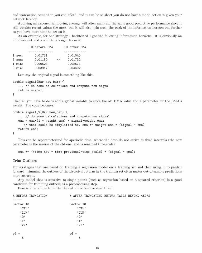
Applying an exponential moving average will often maintain the same good predictive performance since itstill weights recent values the most, but it will also help push the peak of the information horizon out furtherso you have more time to act on it.
As an example, for one strategy I backtested I got the following information horizons. It is obviously animprovement and a shift to a longer horizon:
IC before EMA IC after EMA
------------- ------------
1 sec: 0.01711 0.01040
5 sec: 0.01150 -> 0.01732
1 min: 0.00624 0.02574
5 min: 0.03917 0.04492
Lets say the original signal is something like this:
double signal(Bar new_bar) {
... // do some calculations and compute new signal
return signal;
}
Then all you have to do is add a global variable to store the old EMA value and a parameter for the EMA’sweight. The code becomes:
double signal_2(Bar new_bar) {
... // do some calculations and compute new signal
ema = ema*(1 - weight_ema) + signal*weight_ema;
// that could be simplified to, ema += weight_ema * (signal - ema)
return ema;
}
This can be reparameterized for aperiodic data, where the data do not arrive at fixed intervals (the newparameter is the inverse of the old one, and is renamed time scale):
ema += ((time_now - time_previous)/time_scale) * (signal - ema);
Trim Outliers
For strategies that are based on training a regression model on a training set and then using it to predictforward, trimming the outliers of the historical returns in the training set often makes out-of-sample predictionsmore accurate.
Any model that is sensitive to single points (such as regression based on a squared criterion) is a goodcandidate for trimming outliers as a preprocessing step.
Here is an example from the the output of one backtest I ran:
% BEFORE TRUNCATION % AFTER TRUNCATING RETURN TAILS BEYOND 4SD’S
----- -----
Sector 10 Sector 10
’CTL’ ’CTL’
’LUK’ ’LUK’
’Q’ ’Q’
’T’ ’T’
’VZ’ ’VZ’
pd = pd =
5 5
18
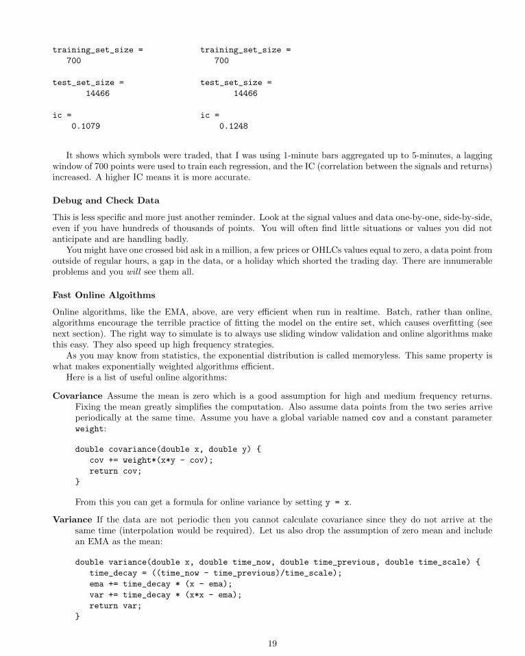
training_set_size = training_set_size =
700 700
test_set_size = test_set_size =
14466 14466
ic = ic =
0.1079 0.1248
It shows which symbols were traded, that I was using 1-minute bars aggregated up to 5-minutes, a laggingwindow of 700 points were used to train each regression, and the IC (correlation between the signals and returns)increased. A higher IC means it is more accurate.
Debug and Check Data
This is less specific and more just another reminder. Look at the signal values and data one-by-one, side-by-side,even if you have hundreds of thousands of points. You will often find little situations or values you did notanticipate and are handling badly.
You might have one crossed bid ask in a million, a few prices or OHLCs values equal to zero, a data point fromoutside of regular hours, a gap in the data, or a holiday which shorted the trading day. There are innumerableproblems and you will see them all.
Fast Online Algoithms
Online algorithms, like the EMA, above, are very efficient when run in realtime. Batch, rather than online,algorithms encourage the terrible practice of fitting the model on the entire set, which causes overfitting (seenext section). The right way to simulate is to always use sliding window validation and online algorithms makethis easy. They also speed up high frequency strategies.
As you may know from statistics, the exponential distribution is called memoryless. This same property iswhat makes exponentially weighted algorithms efficient.
Here is a list of useful online algorithms:
Covariance Assume the mean is zero which is a good assumption for high and medium frequency returns.Fixing the mean greatly simplifies the computation. Also assume data points from the two series arriveperiodically at the same time. Assume you have a global variable named cov and a constant parameterweight:
double covariance(double x, double y) {
cov += weight*(x*y - cov);
return cov;
}
From this you can get a formula for online variance by setting y = x.
Variance If the data are not periodic then you cannot calculate covariance since they do not arrive at thesame time (interpolation would be required). Let us also drop the assumption of zero mean and includean EMA as the mean:
double variance(double x, double time_now, double time_previous, double time_scale) {
time_decay = ((time_now - time_previous)/time_scale);
ema += time_decay * (x - ema);
var += time_decay * (x*x - ema);
return var;
}
19
Note that you may use two different values for the EMA and Variance’s time decay constants.
Linear Regression With Variance and Covariance, we can do linear regression. Assume no intercept, as isthe case when predicting short-term returns. The formula is:
y_predicted = x * cov / var_x;
And we can calculate the standard error of the regression, σ2Y |X . It comes from combinging the two
expressions: σ2xy/σxσy = ρxy, σ
2Y |X = σ2
y ∗ (1− ρ2xy) = σ2y ∗ (1− σ22
xy/σ2xσ
2y)). The formula is:
var_y_given_x = var_y * (1 - cov*cov / (var_x*var_y));
4.9 Machine Learning
Machine learning is a higher level way of coming up with alpha models. You pick a parameterized set ofmodels, input variables, target variable, representative historical dataset, and objective function and then itautomatically picks a certain model.
If you give a machine learning algorithm too much freedom, it will pick a worse model. The model will workwell on the historical data set but poorly in the future. However the whole point of using machine learning isto allow some flexibility. This balance can be studied as a science, but in practice finding the right balance isan art.
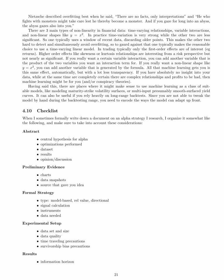
With experience you will get a feel for the “Voodoo Spectrum of Machine Learning”.I used to be very gung-ho about machine learning approaches to trading but I’m less so now. You have to
understand that that there is a spectrum of alpha sources, from very specific structural arbitrage to stat arb tojust voodoo nonsense.
As history goes on, hedge funds and other large players are absorbing the alpha from left to right. Havingsqueezed the pure arbs (ADR vs underlying, ETF vs components, mergers, currency triangles, etc) they thenbecame hungry again and moved to stat arb (momentum, correlated pairs, regression analysis, news sentiment,etc). But now even the big stat arb strategies are running dry so people go further, and sometimes end upchasing mirages (nonlinear regression, causality inference in large data sets, etc).
In modeling the market, it’s best to start with as much structure as possible before moving on to moreflexible statistical strategies. If you have to use statistical machine learning, encode as much trading domainknowledge as possible with specific distance/neighborhood metrics, linearity, variable importance weightings,hierarchy, low-dimensional factors, etc.
It’s good to have a heuristic feel for the danger/flexibility/noise sensitivity (synonyms) of each statisticallearning tool. Here is roughly the “voodoo spectrum” that I have a feel for based on my experience:
Voodoo Spectrum of Machine LearningVery specific, structured, safe
Optimize 1 parameter, require crossvalidation↓
Optimize 2 parameters, require crossvalidation↓
Optimize parameters with too little data, require regularization↓
Extrapolation↓
Nonlinear (SVM, tree bagging, etc)↓
Higher-order variable dependencies↓
Variable selection↓
Structure learningVery general, dangerous in noise, voodoo
20
Nietzsche described overfitting best when he said, “There are no facts, only interpretations” and “He whofights with monsters might take care lest he thereby become a monster. And if you gaze for long into an abyss,the abyss gazes also into you.”
There are 3 main types of non-linearity in financial data: time-varying relationships, variable interactions,and non-linear shapes like y = x2. In practice time-variation is very strong while the other two are lesssignificant. So one typically uses a window of recent data, discarding older points. This makes the other twohard to detect and simultaneously avoid overfitting, so to gaurd against that one typically makes the reasonablechoice to use a time-varying linear model. In trading typically only the first-order effects are of interest (egreturns). Higher order effects like skewness or kurtosis relationships are interesting from a risk perspective butnot nearly as significant. If you really want a certain variable interaction, you can add another variable that isthe product of the two variables you want an interaction term for. If you really want a non-linear shape likey = x2, you can add another variable that is generated by the formula. All that machine learning gets you isthis same effect, automatically, but with a lot less transparency. If you have absolutely no insight into yourdata, while at the same time are completely certain there are complex relationships and profits to be had, thenmachine learning might be for you (and/or conspiracy theories).
Having said this, there are places where it might make sense to use machine learning as a class of suit-able models, like modeling maturity-strike volatility surfaces, or multi-input presumably smooth-surfaced yieldcurves. It can also be useful if you rely heavily on long-range backtests. Since you are not able to tweak themodel by hand during the backtesting range, you need to encode the ways the model can adapt up front.
4.10 Checklist
When I sometimes formally write down a document on an alpha strategy I research, I organize it somewhat likethe following, and make sure to take into account these considerations:
Abstract
• central hypothesis for alpha
• optimizations performed
• dataset
• results
• opinion/discussion
Preliminary Evidence
• charts
• data snapshots
• source that gave you idea
Formal Strategy
• type: model-based, rel value, directional
• signal calculation
• instruments
• data needed
Experimental Setup
• data set and size
• data quality
• time traveling precautions
• survivorship bias precautions
Results
• information horizon
21
• sharpe
• max drawdown
• percent positive days/weeks/months
• correlation to VIX and S&P
• monthly volatility
• average and max leverage
• monthly performance calendar
• returns by day/hour
• equity curve
• big events during test set
Risks
• market regimes
• scenario analysis
• liquidity risk
• time persistance of the arbitrage
• shut-off criteria
Further Work
• estimated capacity
• squeeze more capacity
• hedge/eliminate risks
• get more leverage
• generalize to other asset classes
5 Simulation
If past history was all there was to the game, the richest people would be librarians. –Warren Buffett
Simulation is the number one tool of the quant trader. Simulating a strategy on historic data shows whetherit is likely to make money.
5.1 Data
Periodic “bar” data is the easiest to get. Is sampled at regular intervals (minutely, hourly, daily, weekly) andlooks like this:
Date,Open,High,Low,Close,Volume
11-May-09,33.78,34.72,33.68,34.35,142775884
12-May-09,34.42,34.48,33.52,33.93,147842117
13-May-09,33.63,33.65,32.96,33.02,175548207
14-May-09,33.10,33.70,33.08,33.39,140021617
15-May-09,33.36,33.82,33.23,33.37,121326308
18-May-09,33.59,34.28,33.39,34.24,114333401
19-May-09,34.14,34.74,33.95,34.40,129086394
20-May-09,34.54,35.04,34.18,34.28,131873676
21-May-09,34.02,34.26,33.31,33.65,139253125
“Quote” data shows the best bid and offer:
SYMBOL,DATE,TIME,BID,OFR,BIDSIZ,OFRSIZ
QQQQ,20080509,9:36:26,47.94,47.95,931,964
QQQQ,20080509,9:36:26,47.94,47.95,931,949
22
QQQQ,20080509,9:36:26,47.94,47.95,485,616
QQQQ,20080509,9:36:26,47.94,47.95,485,566
QQQQ,20080509,9:36:26,47.94,47.95,485,576
QQQQ,20080509,9:36:26,47.94,47.95,931,944
QQQQ,20080509,9:36:26,47.94,47.95,849,944
QQQQ,20080509,9:36:26,47.94,47.95,837,944
QQQQ,20080509,9:36:26,47.94,47.95,837,956
“Tick” or “trade” data shows the most recent trades:
SYMBOL,DATE,TIME,PRICE,SIZE
QQQQ,20080509,8:01:29,47.97,1000
QQQQ,20080509,8:01:56,47.97,500
QQQQ,20080509,8:01:56,47.97,237
QQQQ,20080509,8:02:20,47.98,160
QQQQ,20080509,8:02:50,47.98,100
QQQQ,20080509,8:02:50,47.98,200
QQQQ,20080509,8:02:50,47.98,1700
QQQQ,20080509,8:02:50,47.98,500
QQQQ,20080509,8:02:53,47.98,100
“Order book” data shows every order submitted and canceled. If you do not know what it looks like, thenodds are you do not have the resources to be fast enough to trade on it, so do not worry about it.
5.2 Simulators
Here are the most common simulation tools. These are too well known to use space here, so I just give pointersto each and recommend you to google them.
Test Run Time Setup Time Completeness Good ForBacktest Long Long Good EverythingEvent Study Medium Medium Good NewsCorrelation Fast Fast Bad PrototypingPaper Trading Live None Good Production Testing
Backtest
Backtesting is simulating a strategy on historic data and looking at the PnL curve at the end. Basically yourun the strategy like normal, but the data comes from a historical file and time goes as fast as the computercan process.
Event Study
In an event study, you find all the points in time that you have a signal and then average the proceeding andpreceding return paths. This shows you on average what happens before and after. You can see how alphaaccumulates over time and if there is information leakage before the event.
Correlation
The correlation of a signal with future returns is a quick measure of how accuately it predicts. It is betterthan a backtest when you need just a single number to compare strategies, such as for plotting an informationhorizon. You can configure a lagged correlation test in Excel in under a minute. However it doesn’t take intoaccount transaction costs, and it doesn’t output trading-relevant metrics like Sharpe ratio or drawdown.
The information horizon diagram was published in Grinold and Kahn’s Active Portfolio Management. It isa principled way of determining how long to hold positions.
23
Paper Trading
Paper trading refers to trading a strategy through your broker’s API, but using a demo account with fakemoney. It’s good because you can see that the API works, and see if it crashes or if there are data errors. Andit also gives you a better feel for the number of trades it will make and how it will feel emotionally. However ittakes a long time since you have to wait for the markets. It is more practical for high frequency systems whichcan generate a statistically significant number of data points in a short amount of time.
5.3 Pitfalls
Timetravel
When you are testing a strategy on historical data, you have the ability to give it access to more knowledgethan it could possibly have had at that point, like predicting sports with an almanac from the future. Of courseit would be dumb to do that, since it is unrealistic, but usually it is accidental. It is not always easy to notice.If you have a strategy that gives a Sharpe over 3 or so on the first test, you should check very carefully thatyou are not accidentally introducing omniscience. For example, if you use lagged correlation to test a 6-periodmoving average crossover trend-following strategy and use the moving average through time T to predict timeT itself, then you will get a high, but not unreasonable correlation, like .32. It is a hard error to catch and willmake your results during live trading quite disappointing.
Survivorship Bias
If you test a strategy on all the companies in the S&P500 using their prices over the last 10 years, yourbacktest results will be biased. Long-only strategies will have higher returns and short-only will have worsereturns, because the companies that went bankrupt have disappeared from the data set. Even companies whosemarket capitalizations decreased because their prices fell will be missing. You need a data source that includescompanies’ records even after they have gone bankrupt or delisted. Or you need to think very carefully aboutthe strategy you are testing to make sure it is not susceptible to this bias. For an independent trader, the latteris more practical.
Adverse Selection
When executing using limit orders, you will only get filled when someone thinks it will be profitable to trade atyour price. That means every position is slightly more likely to move against you than you may have assumedin simulation.
Instantaneous Communication
It is impossible to trade on a price right when you see it, although this is a common implementation for abacktester. This is mainly a problem for high-frequency systems where communication latency is not negligiblerelative to holding periods.
Transaction Costs
It is also easy to inaccurately estimate transaction costs. Transaction costs change over time, for exampleincreasing when volatility rises and market makers get scared. Market impact also depends on the liquidity ofthe stock, with microcaps being the least liquid.
Unrealistic Backtesting
There are other issues that sometimes cause problems up but are less universal. For example, your data mightnot be high enough resolution to show precisely how the strategy will perform. Another problem is if theexchange does not provide enough data to perfectly reconstruct the book (eg the CME).
24
5.4 Optimization
After developing a strategy and backtesting it, most people try to optimize it. This usually consists of tweakinga parameter, re-running the backtest, keeping the result if the results are better, and repeating multiple times.
If you think about backtesting a strategy, you can see how it could be represented as a function:
profit = backtest_strategy(parameter_1, parameter_2, ...)
Looking at it this way, it is easy to see how to make the computer test all the possible parameter values foryou. Usually it is best to list all the values you want to test for a parameter and try them all (called bruteforce or grid search) rather than to try to save computation time using hill-climbing, simulated annealing, ora genetic algo optimizer.
With hill climbing, you start with a certain parameter value. Then you tweak it by adding a little orsubtracting a little. If it’s an improvement, keep adding until it stops improving. If it’s worsened, then trysubtracting a little and keep subtracting until it stops improving.
Simulated annealing adds one feature to hill climbing. After finding a point where no parameter changeswill help, in simulated annealing you add some random amount to the parameter value and see if it improvesfrom there. This can help “jump” out of a locally optimal parameter setting, which hill climbing would getstuck in.
Genetic algo optimizers add three features. First they run multiple simulated annealings at once withdifferent initial parameter values. The second feature only applies to strategies with multiple parameters. Thegenetic algo periodically stops the set of simulated annealing algos, and creates new ones by combining subsetsof different algo’s parameters. Then it throws away the ones with the least profitable parameter values andstarts extra copies of the most profitable ones. Finally, it creates copies that take a little bit from each of twoprofitable ones. (note: the hill climbing feature is renamed “natural selection,” the simulated annealing featureis renamed “mutation,” the parameter sets are renamed “DNA,” and the sharing feature is called “crossover”)
Let’s see how each of these optimizers looks in a diagram. First, think of the arguments to:
profit = backtest_strategy(parameter_1, parameter_2, ...)
as decimal numbers written in a vector:
| X_1 | X_2 | X_3 | X_4 | X_5 | X_6 | ... | ==> $ Y
Let’s say each X variable is in the range -10 to 10. Let’s say there are only two X variables. Then the bruteforce approach would be (assuming you cut X’s range up into 3 points):
| X_1 | X_2 | ==> $ Y
| -10 | -10 | ==> $ 5
| -10 | 0 | ==> $ 6 best
| -10 | 10 | ==> $ 5
| 0 | -10 | ==> $ 4
| 0 | 0 | ==> $ 5
| 0 | 10 | ==> $ 3
| 10 | -10 | ==> $ 3
| 10 | 0 | ==> $ 3
| 10 | 10 | ==> $ 3
The best point is at (-10,0) so you would take those parameter values. This had 32 combinations we had tobacktest. But let’s say you have 10 parameters. Then there are 310 ≈ 60, 000 combinations and you will wastea lot of time waiting for it to finish.
Hill climbing will proceed like the following. With hill climbing you have to pick a starting point, which wewill say is (0,0), right in the middle of the parameter space. Also we will now change the step size to 5 insteadof 10 since we know this optimizer is more efficient.
| 0 | 0 | ==> $ 5
| 5 | 0 | ==> $ 4 worse, try other direction
25
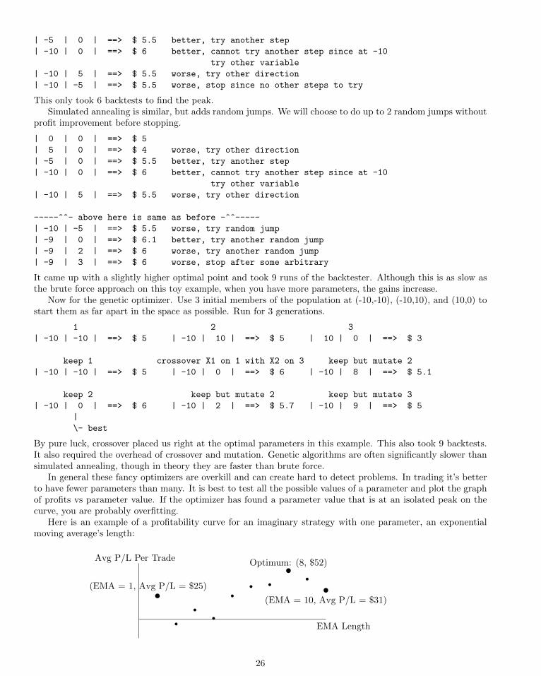
| -5 | 0 | ==> $ 5.5 better, try another step
| -10 | 0 | ==> $ 6 better, cannot try another step since at -10
try other variable
| -10 | 5 | ==> $ 5.5 worse, try other direction
| -10 | -5 | ==> $ 5.5 worse, stop since no other steps to try
This only took 6 backtests to find the peak.Simulated annealing is similar, but adds random jumps. We will choose to do up to 2 random jumps without
profit improvement before stopping.
| 0 | 0 | ==> $ 5
| 5 | 0 | ==> $ 4 worse, try other direction
| -5 | 0 | ==> $ 5.5 better, try another step
| -10 | 0 | ==> $ 6 better, cannot try another step since at -10
try other variable
| -10 | 5 | ==> $ 5.5 worse, try other direction
-----^^- above here is same as before -^^-----
| -10 | -5 | ==> $ 5.5 worse, try random jump
| -9 | 0 | ==> $ 6.1 better, try another random jump
| -9 | 2 | ==> $ 6 worse, try another random jump
| -9 | 3 | ==> $ 6 worse, stop after some arbitrary
It came up with a slightly higher optimal point and took 9 runs of the backtester. Although this is as slow asthe brute force approach on this toy example, when you have more parameters, the gains increase.
Now for the genetic optimizer. Use 3 initial members of the population at (-10,-10), (-10,10), and (10,0) tostart them as far apart in the space as possible. Run for 3 generations.
1 2 3
| -10 | -10 | ==> $ 5 | -10 | 10 | ==> $ 5 | 10 | 0 | ==> $ 3
keep 1 crossover X1 on 1 with X2 on 3 keep but mutate 2
| -10 | -10 | ==> $ 5 | -10 | 0 | ==> $ 6 | -10 | 8 | ==> $ 5.1
keep 2 keep but mutate 2 keep but mutate 3
| -10 | 0 | ==> $ 6 | -10 | 2 | ==> $ 5.7 | -10 | 9 | ==> $ 5
|
\- best
By pure luck, crossover placed us right at the optimal parameters in this example. This also took 9 backtests.It also required the overhead of crossover and mutation. Genetic algorithms are often significantly slower thansimulated annealing, though in theory they are faster than brute force.
In general these fancy optimizers are overkill and can create hard to detect problems. In trading it’s betterto have fewer parameters than many. It is best to test all the possible values of a parameter and plot the graphof profits vs parameter value. If the optimizer has found a parameter value that is at an isolated peak on thecurve, you are probably overfitting.
Here is an example of a profitability curve for an imaginary strategy with one parameter, an exponentialmoving average’s length:
EMA Length
Avg P/L Per Trade
t(EMA = 1, Avg P/L = $25)
r r rr r r tOptimum: (8, $52)r t
(EMA = 10, Avg P/L = $31)
26
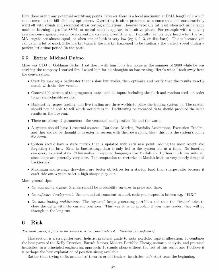
Here there aren’t any potential overfitting points, however there is a local maximum at EMA length of 1 whichcould mess up the hill climbing optimizers. Overfitting is often presented as a curse that one must carefullyward off with rituals and sacrificial stress testing simulations. However typically (at least when not using fancymachine learning algos like SVMs or neural nets) it appears in intuitive places. For example with a movingaverage convergance-divergance momentum strategy, overfitting will typically rear its ugly head when the twoMA lengths are almost equal, or when one or both is very low (eg 1, 2, 3, or 4ish bars). This is because youcan catch a lot of quick little market turns if the market happened to be trading a the perfect speed during aperfect little time period [in the past].
5.5 Extra: Michael Dubno
Mike was CTO of Goldman Sachs. I sat down with him for a few hours in the summer of 2009 while he wasadvising the company I worked for. I asked him for his thoughts on backtesting. Here’s what I took away fromthe conversation:
• Start by making a backtester that is slow but works, then optimize and verify that the results exactlymatch with the slow version.
• Control 100 percent of the program’s state - and all inputs including the clock and random seed - in orderto get reproducible results.
• Backtesting, paper trading, and live trading are three worlds to place the trading system in. The systemshould not be able to tell which world it is in. Backtesting on recorded data should produce the sameresults as the live run.
• There are always 2 parameters - the versioned configuration file and the world.
• A system should have 4 external sources - Database, Market, Portfolio Accountant, Execution Trader -and they should be thought of as external servers with their own config files - this cuts the system’s configfile down.
• System should have a state matrix that is updated with each new point, adding the most recent andforgetting the last. Even in backtesting, data is only fed to the system one at a time. No functioncan query external stats. [This makes interpreted languages like Matlab and Python much less suitable,since loops are generally very slow. The temptation to vectorize in Matlab leads to very poorly designedbacktesters]
• Maximum and average drawdown are better objectives for a startup fund than sharpe ratio because itcan’t ride out 3 years to let a high sharpe play out.
More general tips:
• On combining signals. Signals should be probability surfaces in price and time.
• On software development. Use a standard comment to mark code you suspect is broken e.g. “FIX:”
• On auto-trading architecture. The “system” keeps generating portfolios and then the “trader” tries toclose the delta with the current positions. This way it is no problem if you miss trades, they will gothrough in the long run.
6 Risk
The most powerful force in the universe is compound interest. –Einstein (unconfirmed)
This section is a straightforward, holistic, practical guide to risky portfolio capital allocation. It combinesthe best parts of the Kelly Criterion, Barra’s factors, Modern Portfolio Theory, scenario analysis, and practicalheuristics, in a principled engineering approach. It stands alone without the rest of this script and I believe itis perhaps the best explanation of position sizing available.
Rather than trying to fix academics’ theories or old traders’ heuristics, let’s start from the beginning.
27
6.1 Single Strategy Allocation
Assume you have a strategy that is profitable, otherwise, bet $0. How do you make as much money as possible?Assume you have $100 to trade with– your total net worth including everything anyone would loan you. Putall your money into it? No, then on the first losing trade you go to $0. Put 99% of your money in it? No, thenon the first losing trade you go to $1, and even a 100% winner after that only brings you to $2, down a net of$98. Put 98% in it? No then you still go down too much on losers. Put 1% in it? No then you barely make anymoney. Clearly there is an optimization problem here, with a curve we are starting to uncover. It has minimaaround 0% and 100% and a peak somewhere in between.
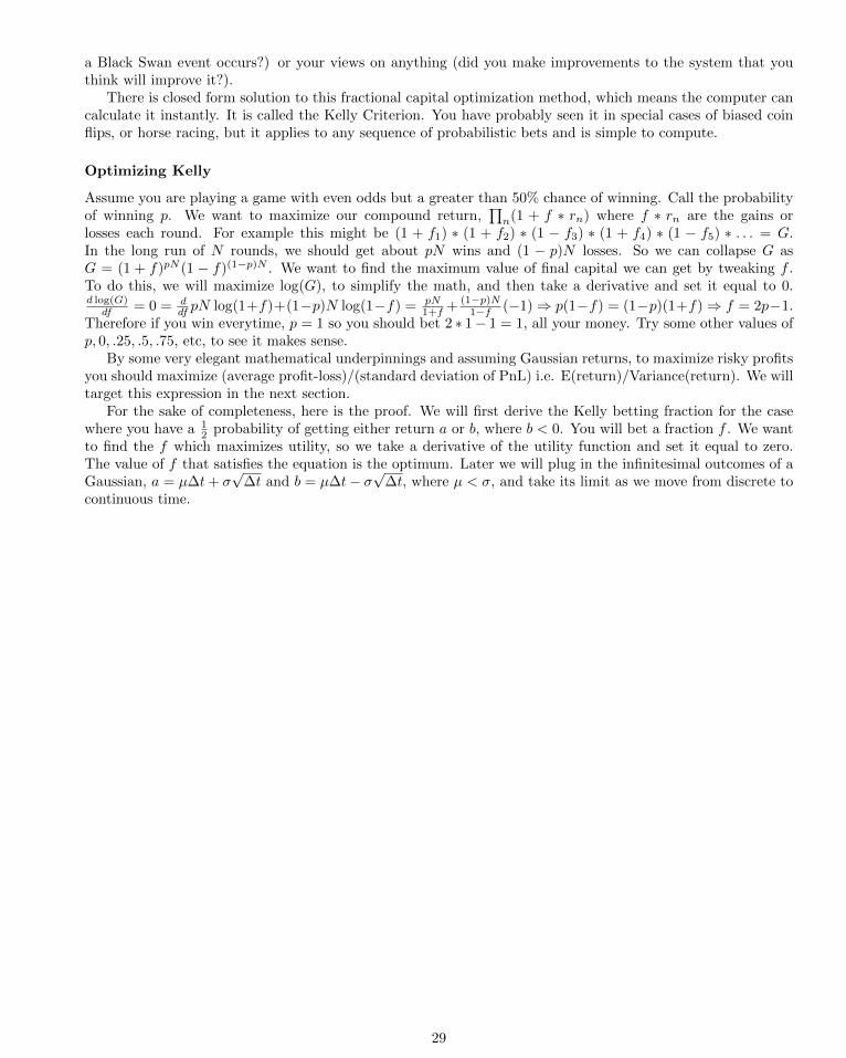
Skewed die roll
Consider the case where you are trying to find the best amount to bet on a game where you roll a die andwin 1 on any number but 6, and lose 4 on a 6. This is a good strategy because on average you make money5/6 ∗ 1− 1/6 ∗ 4 = 1/6 > 0. Let’s look at a graph of the PnL from betting on this game 100 times with differentamounts of your capital. In R, type:
X = rep(1,100);
X[which(rbinom(100, 1, 1/6)==1)] = -4;
profit = function(f)prod(1+f*X);
fs = seq(0,2/24,1/24/10);
profits = sapply(fs, profit);
plot(fs, profits, main=’Optimum Profit’)
We have plotted all levels of leverage between 0 and 1/12:
y(0.0%, 0.0%)
t t t t t t t
(% Leverage, % Return)
t yOptimum: (3.75%, 7.82%)t t t t t t tt
tty(0.0833%, -6.641%)
Backtesting
You need to optimize your position size in a principled, consistent method. First you need more detailedassumptions. Assume the strategies profits and losses are governed by probability, rather than deterministicor determined adversarially. Assume this distribution is the same on each trade (we’ll get rid of this obviouslyimpossible to satisfy assumption later). Now optimize based on the results of a backtest. Assume the samefraction of your total capital was placed into each trade. Take the sequence of profits and losses and calculatewhat fraction would have resulted in the most profit. Think of the backtest PnL as the sequence of die rollsyou get playing the previous game, and position sizing as optimizing the curve above.
You are right if you think solely looking at the past is silly. You can freely add in imaginary PnLs whichyou think are likely to happen in the future. Add them in proportion to the frequency that you think they willoccur so the math doesn’t become biased. These imaginary PnLs could be based on scenario analysis (what if
28
a Black Swan event occurs?) or your views on anything (did you make improvements to the system that youthink will improve it?).
There is closed form solution to this fractional capital optimization method, which means the computer cancalculate it instantly. It is called the Kelly Criterion. You have probably seen it in special cases of biased coinflips, or horse racing, but it applies to any sequence of probabilistic bets and is simple to compute.
Optimizing Kelly
Assume you are playing a game with even odds but a greater than 50% chance of winning. Call the probabilityof winning p. We want to maximize our compound return,
∏n(1 + f ∗ rn) where f ∗ rn are the gains or
losses each round. For example this might be (1 + f1) ∗ (1 + f2) ∗ (1 − f3) ∗ (1 + f4) ∗ (1 − f5) ∗ . . . = G.In the long run of N rounds, we should get about pN wins and (1 − p)N losses. So we can collapse G asG = (1 + f)pN (1 − f)(1−p)N . We want to find the maximum value of final capital we can get by tweaking f .To do this, we will maximize log(G), to simplify the math, and then take a derivative and set it equal to 0.d log(G)
df = 0 = ddf pN log(1+f)+(1−p)N log(1−f) = pN
1+f + (1−p)N1−f (−1)⇒ p(1−f) = (1−p)(1+f)⇒ f = 2p−1.
Therefore if you win everytime, p = 1 so you should bet 2 ∗ 1− 1 = 1, all your money. Try some other values ofp, 0, .25, .5, .75, etc, to see it makes sense.
By some very elegant mathematical underpinnings and assuming Gaussian returns, to maximize risky profitsyou should maximize (average profit-loss)/(standard deviation of PnL) i.e. E(return)/Variance(return). We willtarget this expression in the next section.
For the sake of completeness, here is the proof. We will first derive the Kelly betting fraction for the casewhere you have a 1
2 probability of getting either return a or b, where b < 0. You will bet a fraction f . We wantto find the f which maximizes utility, so we take a derivative of the utility function and set it equal to zero.The value of f that satisfies the equation is the optimum. Later we will plug in the infinitesimal outcomes of aGaussian, a = µ∆t+ σ
√∆t and b = µ∆t− σ
√∆t, where µ < σ, and take its limit as we move from discrete to
continuous time.
29
0 =d
df(.5 log(1 + fa) + .5 log(1 + fb))
=d
df(log(1 + fa) + log(1 + fb)) multiply both sides by 2
=a
1 + fa+
b
1 + fbderivative, chain rule
=a(1 + fb) + b(1 + fa)
(1 + fa)(1 + fb)common denominator
= a(1 + fb) + b(1 + fa) multiply by the denominator
= a+ fab+ b+ fab distribute
⇐⇒ −2fab = a+ b subtract 2fab
⇐⇒ f =a+ b
− 2abdivide by− 2ab
=µ∆t+ σ
√∆t+ µ∆t− σ
√∆t
− 2(µ∆t+ σ√
∆t)(µ∆t− σ√
∆t)plugging in a, b
=2µ∆t
− 2((µ∆t)2 − (σ√
∆t)2)simplify with algebra
=µ∆t
σ2∆t− µ2(∆t)2simplify more with algebra
=µ
σ2 − µ2∆tcancelling ∆t
→ µ
σ2limit as ∆t→ 0
6.2 Multiple Strategies
Assume now that you have multiple profitable strategies. You can decrease the risk of your net position byallocating parts of your capital to strategies with risks that cancel each other out. Even putting money in astrategy with lower expected profit can help out because the benefits of canceling risk are initially more powerfulthan sacrificing some profit. With less risk, you can invest a higher fraction of your capital and make profits offof the extra part you invest rather than sidelining it.
To balance position sizes in multiple strategies in a principled fashion requires more mathematical sophis-tication. Let
∑(wiXi) be the portfolio represented as a random variable. The uncertain numbers (random
variables) Xi are the PnL distributions of each strategy. The numbers wi are the fractions of your investedcapital in each strategy. The sum of all wi is 1. The expected return is then E(
∑wiXi) =
∑E(wiXi), which
is easy to maximize. The risk is then Var(∑wiXi) =
∑w2
i Var(Xi) +∑∑
wiwjCovariance(Xi, Xj). Covari-ance is the shared risk between the two strategies. Covariance can be broken down into standard deviationand correlation since Covariance(Xi, Xj) = SD(Xi)SD(Xj)Correlation(Xi, Xj). The portfolio variance is moreinteresting than the expected profit, since by changing the weights we can decrease it substantially.
Covariance as coin flipping from 2 pools
The intuition behind correlation is simple. Say two random variables X1 and X2 are generated by flipping 10coins each. If they are uncorrelated, then we flip the 10 coins separately for X1 and X2. If we flip the 10coins to first generate X1, and then leave 1 coin lying down and only flip the other 9 when generating X2, thenCorrelation(X1, X2) = 1/10 = .1. If we don’t touch 2 coins and only reflip 8 of them for X2, then the correlationwill be 2/10. In terms of trading strategies, you can imagine that the coins in common represent common riskfactor exposures. For example stocks typically have correlation to the overall market of about .5 − .8. This isequivalent to saying that after generating the overall market returns by flipping 10 coins, you only pick up and
30
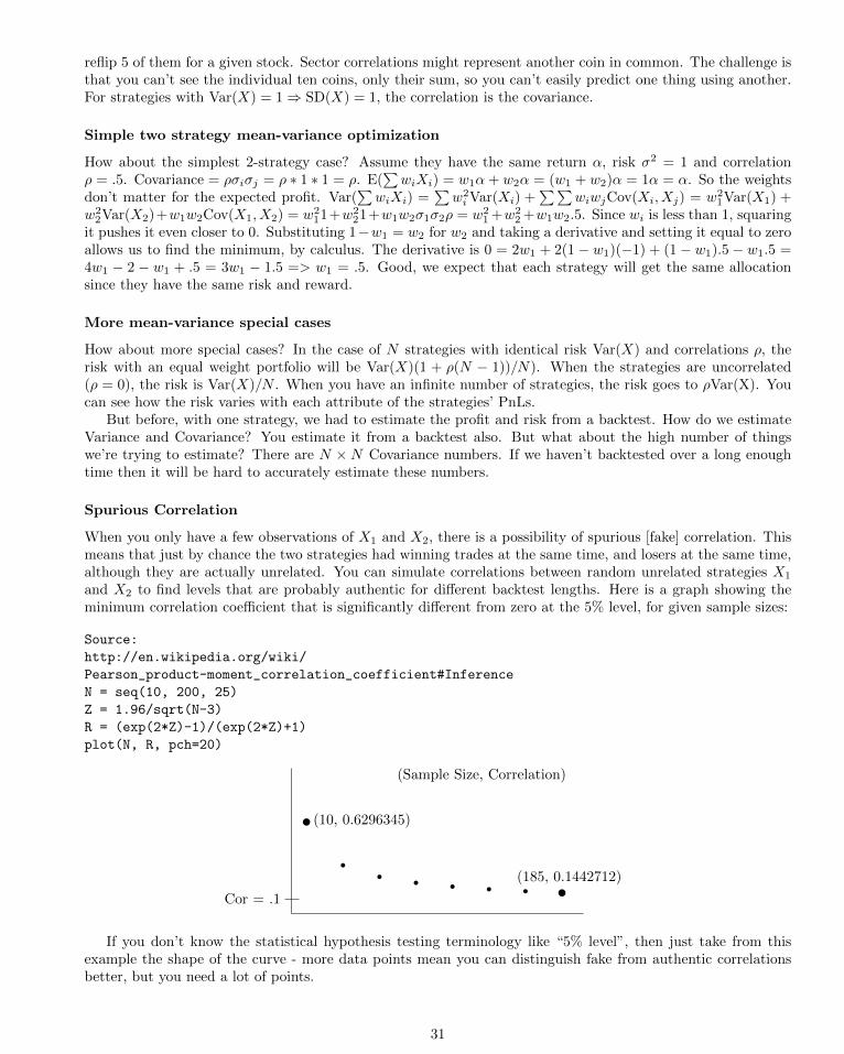
reflip 5 of them for a given stock. Sector correlations might represent another coin in common. The challenge isthat you can’t see the individual ten coins, only their sum, so you can’t easily predict one thing using another.For strategies with Var(X) = 1⇒ SD(X) = 1, the correlation is the covariance.
Simple two strategy mean-variance optimization
How about the simplest 2-strategy case? Assume they have the same return α, risk σ2 = 1 and correlationρ = .5. Covariance = ρσiσj = ρ ∗ 1 ∗ 1 = ρ. E(
∑wiXi) = w1α+ w2α = (w1 + w2)α = 1α = α. So the weights
don’t matter for the expected profit. Var(∑wiXi) =
∑w2
i Var(Xi) +∑∑
wiwjCov(Xi, Xj) = w21Var(X1) +
w22Var(X2)+w1w2Cov(X1, X2) = w2
11+w221+w1w2σ1σ2ρ = w2
1 +w22 +w1w2.5. Since wi is less than 1, squaring
it pushes it even closer to 0. Substituting 1−w1 = w2 for w2 and taking a derivative and setting it equal to zeroallows us to find the minimum, by calculus. The derivative is 0 = 2w1 + 2(1 − w1)(−1) + (1 − w1).5 − w1.5 =4w1 − 2 − w1 + .5 = 3w1 − 1.5 => w1 = .5. Good, we expect that each strategy will get the same allocationsince they have the same risk and reward.
More mean-variance special cases
How about more special cases? In the case of N strategies with identical risk Var(X) and correlations ρ, therisk with an equal weight portfolio will be Var(X)(1 + ρ(N − 1))/N). When the strategies are uncorrelated(ρ = 0), the risk is Var(X)/N . When you have an infinite number of strategies, the risk goes to ρVar(X). Youcan see how the risk varies with each attribute of the strategies’ PnLs.
But before, with one strategy, we had to estimate the profit and risk from a backtest. How do we estimateVariance and Covariance? You estimate it from a backtest also. But what about the high number of thingswe’re trying to estimate? There are N ×N Covariance numbers. If we haven’t backtested over a long enoughtime then it will be hard to accurately estimate these numbers.
Spurious Correlation
When you only have a few observations of X1 and X2, there is a possibility of spurious [fake] correlation. Thismeans that just by chance the two strategies had winning trades at the same time, and losers at the same time,although they are actually unrelated. You can simulate correlations between random unrelated strategies X1
and X2 to find levels that are probably authentic for different backtest lengths. Here is a graph showing theminimum correlation coefficient that is significantly different from zero at the 5% level, for given sample sizes:
Source:
http://en.wikipedia.org/wiki/
Pearson_product-moment_correlation_coefficient#Inference
N = seq(10, 200, 25)
Z = 1.96/sqrt(N-3)
R = (exp(2*Z)-1)/(exp(2*Z)+1)
plot(N, R, pch=20)
(Sample Size, Correlation)
t(10, 0.6296345)
r r r r r r t(185, 0.1442712)
Cor = .1
If you don’t know the statistical hypothesis testing terminology like “5% level”, then just take from thisexample the shape of the curve - more data points mean you can distinguish fake from authentic correlationsbetter, but you need a lot of points.
31
You need to decrease the number of parameters. Academics and traders have come up with tons of differentways of doing this. There are problems with most methods. Before you get lost in the trees of the forest,remember that you are trying to balance strategies’ PnLs so their risks cancel out, so that you can safely put abigger fraction of your capital to work. Estimating which strategies’ risks cancel out is hard to do because thenumber of pairings of N strategies is N ×N and you only have a limited amount of backtest data. Here are thekey ideas behind each approach:
1. Buy it from Barra to pass on the blame BARRA was started in 1974 to improve portfolio constuction.They were the first to predict covariances rather than just base them on historical data. They alsoexplained covariance (beta) in terms of fundamental risk factors to make the quantitative approach morepalatable to portfolio managers.
2. Factor Model A matrix like the covariance matrix can be broken up into columns or rows. Rather thanhaving the matrix derived from the strategies themselves, you can have it based on a smaller number ofintuitive components such as a stock sector, commodity, or interest rate. So instead of having to estimateN ×N numbers, you will have N × F where F is the number of factors and hopefully less than N . Theimportant thing is that the factors are independent in the linear algebra sense.
3. Regularization The covariance matrix has variance terms along the diagonal and covariance terms offthe diagonal. It is the covariance terms that will mess up position sizing. This is because there are alot more of them and because having the wrong covariance number effects two strategies, not just 1, andit can affect them a lot if the covariance comes out negative. In regularization you take a weighted sumof the sample covariance matrix and the identity matrix. This decreases the influence of the covarianceterms and balances the position sizes to be more even across all strategies.
4. Bootstrap Bootstrapping is a way of estimating the error in your covariance number. In this method,you take B random subsamples of the strategies’ PnL curves and calculate the covariance of these samples.After doing this you will get B covariance numbers, all a little bit different depending on which pointswere excluded. Typically then one will take the number which is closest to 0. Choosing covariances closerto 0 balances out the strategies’ allocations.
5. Universal Portfolio A product of game theory and information theory (which was also the origin ofthe Kelly Criterion), the universal portfolio approach attempts to minimize the difference between theperformance of the portfolio of strategies and the best strategy in the portfolio from the very first trade(including simulated trades). It does not give the kind of performance we want since it seeks minimaxoptimality rather than in-expectation optimality.
6. Scenario Analysis The covariance term numerically represents how the two strategies will move togetherin the future. Future movements are driven by human events. Listing the most probable scenarios alongwith their probabilities and anticipated effects on each strategy is another principled way to calculatecovariance. This is most appropriate for long-term fundamental investors.
7. Random Matrix Theory Random matrix theory has two components. The first contribution is amethod to estimate the typical level of spurious correlations by measuring the average correlation betweenuncorrelated random sequences. Making this precise in the case of N ×N correlations is the interestingcase. The second contribution is a method to extract the true correlations by building the covariancematrix from the largest eigenvalue eigenvectors (and throwing away the rest) of the sample covariance.
8. Realized Variance By using higher frequency data to construct the covariance matrix, you can get moredatapoints so there’s less risk of spurious correlation. The relationships between strategies that exist athigh frequencies typically also hold at lower frequencies. This has been termed “realized variance.” Whenyou go to very high frequency data, problems arise because trades actually occur asyncronously, not atfixed periods like OHLC-bar data. As long as you stay above 5-min bars for large caps and 30-min barsfor small caps, the realized variance approach to high frequency covariance estimation will work well.However you need access to higher frequency bars and the infrastructure to trade at multiple horizons.
32
9. Equal Weight Portfolio :( If you become pessimistic on all this complicated estimation nonsense andjust want to get on with trading, the the 1/N portfolio is for you. 1/N means you just allocate equalamounts to each strategy. A lot of academic research shows that this allocation beats fancier methodswhen you go out of the training data.
10. Decompose and Forecasts Covariance is really some part of each of the approaches above. The rightthing to do is fuse them all. Covariance = V ariance ∗ Correlation.
V ariance is predictable, and even very short term exponentially weighted dynamic linear forecasting canperform very well, predicting about 30% of the hourly changes using a 10 minute window. Incorporatingchanges in spreads and implied volatilities provides another marginal improvement. News will improve ittoo.
Correlation is a matrix decomposable into factor vectors corresponding to noise and to fundamentalfactors, which will result from the future’s scenario, but it is affected by sampling error. Statistical andscenario-based forecasts of the factors’ correlations will improve portfolio risk estimates. Isolating the noisein the matrix and smoothing globally prevents overfitting to the risk estimates. Correlation should bestatistically predicted using exponentially weighted windows of 1 week of 1-minute data. A simple linearfactor models on related assets’ prices is sufficient for another significant fundamentals-based improvement.
6.3 Porfolio Allocation Summary
After you get the expected returns, variances, and covariances, you are ready to allocate capital to multiplestrategies. After getting the right weights for each strategy, treat the strategy portfolio as a single strategy andapply the Kelly Criterion optimization to the net strategies’ PnL. If you don’t like any of the numbers that popout from the formulas or backtest, feel free to modify them. If you see a correlation at 0.2 and you think 0.5 ismore reasonable, change it. The numbers are only estimates based on the past. If you have some insight to thefuture, feel free to apply it.
There are still unanswered questions which I will briefly answer here.If you have strategies that trade over different horizons, what horizon should the strategy portfolio use?
Calculate the risk at the longer horizon but use separate estimators optimized for each horizon.How can you tell if your principled estimation recipe worked? Compare it to an alternative method. How do
you compare them? The general approach is to calculate the 1-period realized risk at the horizon for multiplesets of random weights; a more specific approach is appropriate for other objectives - such as constructingminimum variance portfolios.
6.4 Extra: Empirical Kelly Code
The following Kelly optimization code is very general and useful for the case when your strategy has very skewedor fat tailed returns. I have not seen it published anywhere else so I include it here.
"""
These python functions are used to calculate the growth-optimal
leverage for a strategy based on its backtest performance. Each
trade’s profit or loss is treated as one sample from an underlying
probability distribution which is generating the PnLs. This function
optimizes the amount of leverage one would use when betting on this
distribution, assuming that the strategy will have the same performance
in the near future.
Example:
# Load some data from yahoo
import matplotlib.finance as fin
import datetime as dt
33
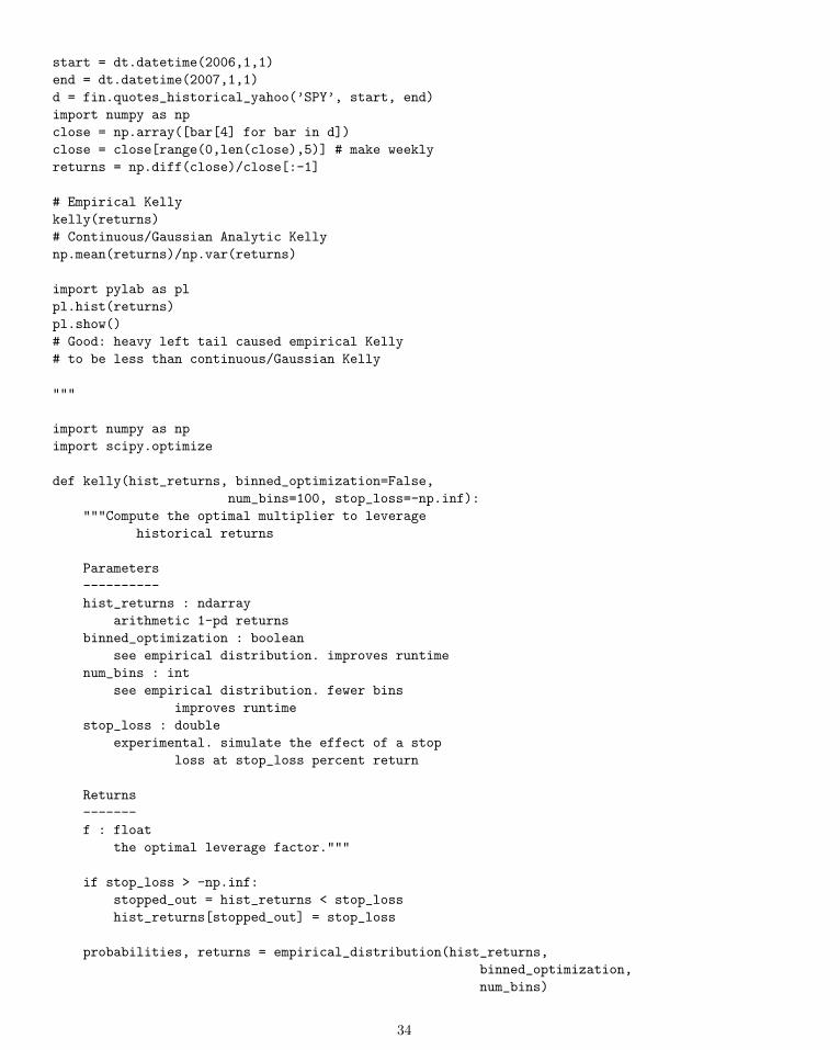
start = dt.datetime(2006,1,1)
end = dt.datetime(2007,1,1)
d = fin.quotes_historical_yahoo(’SPY’, start, end)
import numpy as np
close = np.array([bar[4] for bar in d])
close = close[range(0,len(close),5)] # make weekly
returns = np.diff(close)/close[:-1]
# Empirical Kelly
kelly(returns)
# Continuous/Gaussian Analytic Kelly
np.mean(returns)/np.var(returns)
import pylab as pl
pl.hist(returns)
pl.show()
# Good: heavy left tail caused empirical Kelly
# to be less than continuous/Gaussian Kelly
"""
import numpy as np
import scipy.optimize
def kelly(hist_returns, binned_optimization=False,
num_bins=100, stop_loss=-np.inf):
"""Compute the optimal multiplier to leverage
historical returns
Parameters
----------
hist_returns : ndarray
arithmetic 1-pd returns
binned_optimization : boolean
see empirical distribution. improves runtime
num_bins : int
see empirical distribution. fewer bins
improves runtime
stop_loss : double
experimental. simulate the effect of a stop
loss at stop_loss percent return
Returns
-------
f : float
the optimal leverage factor."""
if stop_loss > -np.inf:
stopped_out = hist_returns < stop_loss
hist_returns[stopped_out] = stop_loss
probabilities, returns = empirical_distribution(hist_returns,
binned_optimization,
num_bins)
34
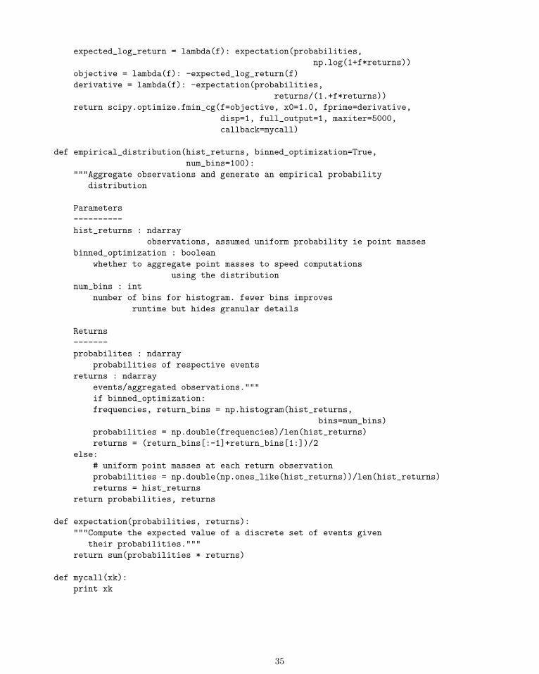
expected_log_return = lambda(f): expectation(probabilities,
np.log(1+f*returns))
objective = lambda(f): -expected_log_return(f)
derivative = lambda(f): -expectation(probabilities,
returns/(1.+f*returns))
return scipy.optimize.fmin_cg(f=objective, x0=1.0, fprime=derivative,
disp=1, full_output=1, maxiter=5000,
callback=mycall)
def empirical_distribution(hist_returns, binned_optimization=True,
num_bins=100):
"""Aggregate observations and generate an empirical probability
distribution
Parameters
----------
hist_returns : ndarray
observations, assumed uniform probability ie point masses
binned_optimization : boolean
whether to aggregate point masses to speed computations
using the distribution
num_bins : int
number of bins for histogram. fewer bins improves
runtime but hides granular details
Returns
-------
probabilites : ndarray
probabilities of respective events
returns : ndarray
events/aggregated observations."""
if binned_optimization:
frequencies, return_bins = np.histogram(hist_returns,
bins=num_bins)
probabilities = np.double(frequencies)/len(hist_returns)
returns = (return_bins[:-1]+return_bins[1:])/2
else:
# uniform point masses at each return observation
probabilities = np.double(np.ones_like(hist_returns))/len(hist_returns)
returns = hist_returns
return probabilities, returns
def expectation(probabilities, returns):
"""Compute the expected value of a discrete set of events given
their probabilities."""
return sum(probabilities * returns)
def mycall(xk):
print xk
35
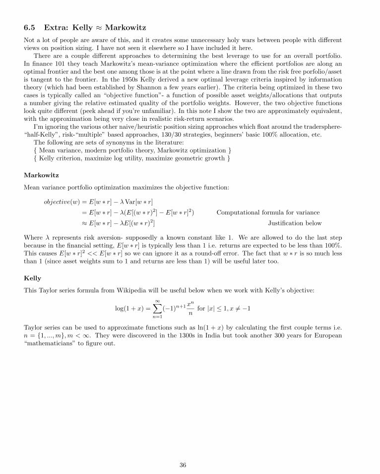
6.5 Extra: Kelly ≈ Markowitz
Not a lot of people are aware of this, and it creates some unnecessary holy wars between people with differentviews on position sizing. I have not seen it elsewhere so I have included it here.
There are a couple different approaches to determining the best leverage to use for an overall portfolio.In finance 101 they teach Markowitz’s mean-variance optimization where the efficient portfolios are along anoptimal frontier and the best one among those is at the point where a line drawn from the risk free porfolio/assetis tangent to the frontier. In the 1950s Kelly derived a new optimal leverage criteria inspired by informationtheory (which had been established by Shannon a few years earlier). The criteria being optimized in these twocases is typically called an “objective function”- a function of possible asset weights/allocations that outputsa number giving the relative estimated quality of the portfolio weights. However, the two objective functionslook quite different (peek ahead if you’re unfamiliar). In this note I show the two are approximately equivalent,with the approximation being very close in realistic risk-return scenarios.
I’m ignoring the various other naive/heuristic position sizing approaches which float around the tradersphere-“half-Kelly”, risk-“multiple” based approaches, 130/30 strategies, beginners’ basic 100% allocation, etc.
The following are sets of synonyms in the literature:{ Mean variance, modern portfolio theory, Markowitz optimization }{ Kelly criterion, maximize log utility, maximize geometric growth }
Markowitz
Mean variance portfolio optimization maximizes the objective function:
objective(w) = E[w ∗ r]− λVar[w ∗ r]= E[w ∗ r]− λ(E[(w ∗ r)2]− E[w ∗ r]2) Computational formula for variance
≈ E[w ∗ r]− λE[(w ∗ r)2] Justification below
Where λ represents risk aversion- supposedly a known constant like 1. We are allowed to do the last stepbecause in the financial setting, E[w ∗ r] is typically less than 1 i.e. returns are expected to be less than 100%.This causes E[w ∗ r]2 << E[w ∗ r] so we can ignore it as a round-off error. The fact that w ∗ r is so much lessthan 1 (since asset weights sum to 1 and returns are less than 1) will be useful later too.
Kelly
This Taylor series formula from Wikipedia will be useful below when we work with Kelly’s objective:
log(1 + x) =
∞∑n=1
(−1)n+1xn
nfor |x| ≤ 1, x 6= −1
Taylor series can be used to approximate functions such as ln(1 + x) by calculating the first couple terms i.e.n = {1, ...,m},m < ∞. They were discovered in the 1300s in India but took another 300 years for European“mathematicians” to figure out.
36
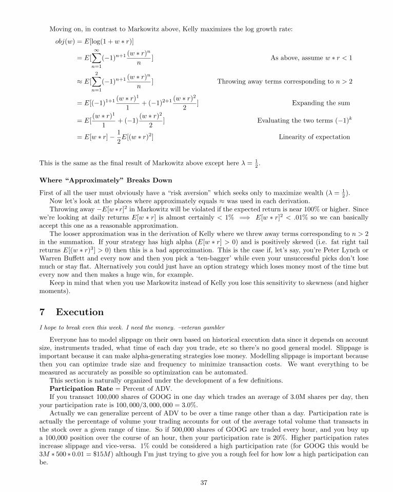
Moving on, in contrast to Markowitz above, Kelly maximizes the log growth rate:
obj(w) = E[log(1 + w ∗ r)]
= E[
∞∑n=1
(−1)n+1 (w ∗ r)n
n] As above, assume w ∗ r < 1
≈ E[
2∑n=1
(−1)n+1 (w ∗ r)n
n] Throwing away terms corresponding to n > 2
= E[(−1)1+1 (w ∗ r)1
1+ (−1)2+1 (w ∗ r)2
2] Expanding the sum
= E[(w ∗ r)1
1+ (−1)
(w ∗ r)2
2] Evaluating the two terms (−1)k
= E[w ∗ r]− 1
2E[(w ∗ r)2] Linearity of expectation
This is the same as the final result of Markowitz above except here λ = 12 .
Where “Approximately” Breaks Down
First of all the user must obviously have a “risk aversion” which seeks only to maximize wealth (λ = 12 ).
Now let’s look at the places where approximately equals ≈ was used in each derivation.Throwing away −E[w∗r]2 in Markowitz will be violated if the expected return is near 100% or higher. Since
we’re looking at daily returns E[w ∗ r] is almost certainly < 1% =⇒ E[w ∗ r]2 < .01% so we can basicallyaccept this one as a reasonable approximation.
The looser approximation was in the derivation of Kelly where we threw away terms corresponding to n > 2in the summation. If your strategy has high alpha (E[w ∗ r] > 0) and is positively skewed (i.e. fat right tailreturns E[(w ∗ r)3] > 0) then this is a bad approximation. This is the case if, let’s say, you’re Peter Lynch orWarren Buffett and every now and then you pick a ‘ten-bagger’ while even your unsuccessful picks don’t losemuch or stay flat. Alternatively you could just have an option strategy which loses money most of the time butevery now and then makes a huge win, for example.
Keep in mind that when you use Markowitz instead of Kelly you lose this sensitivity to skewness (and highermoments).
7 Execution
I hope to break even this week. I need the money. –veteran gambler
Everyone has to model slippage on their own based on historical execution data since it depends on accountsize, instruments traded, what time of each day you trade, etc so there’s no good general model. Slippage isimportant because it can make alpha-generating strategies lose money. Modelling slippage is important becausethen you can optimize trade size and frequency to minimize transaction costs. We want everything to bemeasured as accurately as possible so optimization can be automated.
This section is naturally organized under the development of a few definitions.Participation Rate = Percent of ADV.If you transact 100,000 shares of GOOG in one day which trades an average of 3.0M shares per day, then
your participation rate is 100, 000/3, 000, 000 = 3.0%.Actually we can generalize percent of ADV to be over a time range other than a day. Participation rate is
actually the percentage of volume your trading accounts for out of the average total volume that transacts inthe stock over a given range of time. So if 500,000 shares of GOOG are traded every hour, and you buy upa 100,000 position over the course of an hour, then your participation rate is 20%. Higher participation ratesincrease slippage and vice-versa. 1% could be considered a high participation rate (for GOOG this would be3M ∗ 500 ∗ 0.01 = $15M) although I’m just trying to give you a rough feel for how low a high participation canbe.
37
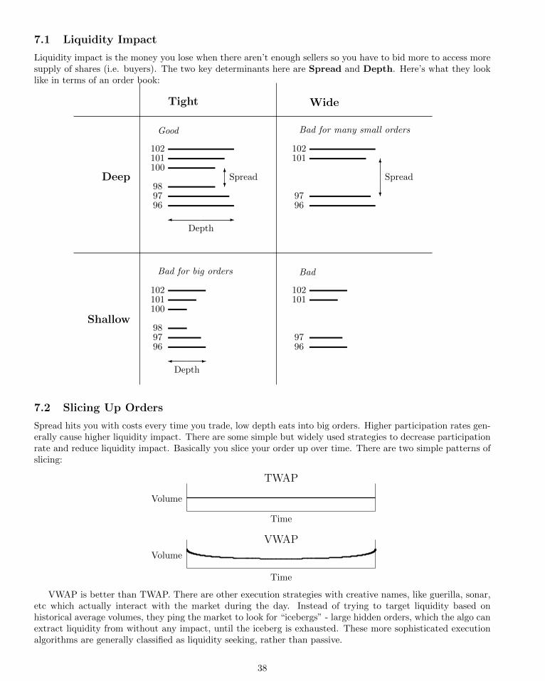
7.1 Liquidity Impact
Liquidity impact is the money you lose when there aren’t enough sellers so you have to bid more to access moresupply of shares (i.e. buyers). The two key determinants here are Spread and Depth. Here’s what they looklike in terms of an order book:
Tight
Deep
Good
102101100
6?Spread
989796
-�Depth
Wide
Bad for many small orders
102101
6
?
Spread
9796
Bad for big orders
Shallow
102101100
989796
-�Depth
Bad
102101
9796
7.2 Slicing Up Orders
Spread hits you with costs every time you trade, low depth eats into big orders. Higher participation rates gen-erally cause higher liquidity impact. There are some simple but widely used strategies to decrease participationrate and reduce liquidity impact. Basically you slice your order up over time. There are two simple patterns ofslicing:
Volume
Time
Volume
Time
TWAP
VWAP
VWAP is better than TWAP. There are other execution strategies with creative names, like guerilla, sonar,etc which actually interact with the market during the day. Instead of trying to target liquidity based onhistorical average volumes, they ping the market to look for “icebergs” - large hidden orders, which the algo canextract liquidity from without any impact, until the iceberg is exhausted. These more sophisticated executionalgorithms are generally classified as liquidity seeking, rather than passive.
38
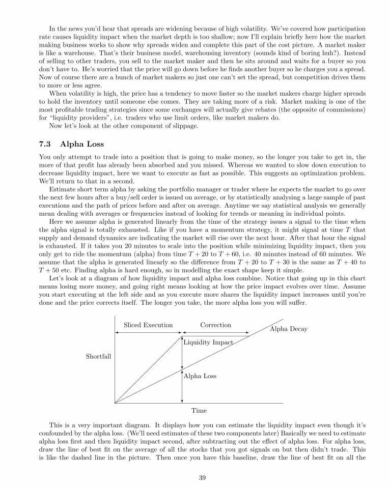
In the news you’d hear that spreads are widening because of high volatility. We’ve covered how participationrate causes liquidity impact when the market depth is too shallow; now I’ll explain briefly here how the marketmaking business works to show why spreads widen and complete this part of the cost picture. A market makeris like a warehouse. That’s their business model, warehousing inventory (sounds kind of boring huh?). Insteadof selling to other traders, you sell to the market maker and then he sits around and waits for a buyer so youdon’t have to. He’s worried that the price will go down before he finds another buyer so he charges you a spread.Now of course there are a bunch of market makers so just one can’t set the spread, but competition drives themto more or less agree.
When volatility is high, the price has a tendency to move faster so the market makers charge higher spreadsto hold the inventory until someone else comes. They are taking more of a risk. Market making is one of themost profitable trading strategies since some exchanges will actually give rebates (the opposite of commissions)for “liquidity providers”, i.e. traders who use limit orders, like market makers do.
Now let’s look at the other component of slippage.
7.3 Alpha Loss
You only attempt to trade into a position that is going to make money, so the longer you take to get in, themore of that profit has already been absorbed and you missed. Whereas we wanted to slow down execution todecrease liquidity impact, here we want to execute as fast as possible. This suggests an optimization problem.We’ll return to that in a second.
Estimate short term alpha by asking the portfolio manager or trader where he expects the market to go overthe next few hours after a buy/sell order is issued on average, or by statistically analysing a large sample of pastexecutions and the path of prices before and after on average. Anytime we say statistical analysis we generallymean dealing with averages or frequencies instead of looking for trends or meaning in individual points.
Here we assume alpha is generated linearly from the time of the strategy issues a signal to the time whenthe alpha signal is totally exhausted. Like if you have a momentum strategy, it might signal at time T thatsupply and demand dynamics are indicating the market will rise over the next hour. After that hour the signalis exhausted. If it takes you 20 minutes to scale into the position while minimizing liquidity impact, then youonly get to ride the momentum (alpha) from time T + 20 to T + 60, i.e. 40 minutes instead of 60 minutes. Weassume that the alpha is generated linearly so the difference from T + 20 to T + 30 is the same as T + 40 toT + 50 etc. Finding alpha is hard enough, so in modelling the exact shape keep it simple.
Let’s look at a diagram of how liquidity impact and alpha loss combine. Notice that going up in this chartmeans losing more money, and going right means looking at how the price impact evolves over time. Assumeyou start executing at the left side and as you execute more shares the liquidity impact increases until you’redone and the price corrects itself. The longer you take, the more alpha loss you will suffer.
Shortfall
Time
� -Sliced Execution
� -Correction
?
6Liquidity Impact
?
6Alpha Loss
����������
���
���
���
���
���
���
���
���
�
Alpha Decay
This is a very important diagram. It displays how you can estimate the liquidity impact even though it’sconfounded by the alpha loss. (We’ll need estimates of these two components later) Basically we need to estimatealpha loss first and then liquidity impact second, after subtracting out the effect of alpha loss. For alpha loss,draw the line of best fit on the average of all the stocks that you got signals on but then didn’t trade. Thisis like the dashed line in the picture. Then once you have this baseline, draw the line of best fit on all the
39
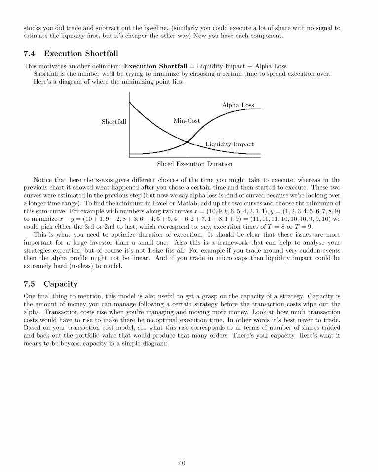
stocks you did trade and subtract out the baseline. (similarly you could execute a lot of share with no signal toestimate the liquidity first, but it’s cheaper the other way) Now you have each component.
7.4 Execution Shortfall
This motivates another definition: Execution Shortfall = Liquidity Impact + Alpha LossShortfall is the number we’ll be trying to minimize by choosing a certain time to spread execution over.Here’s a diagram of where the minimizing point lies:
Shortfall
Sliced Execution Duration
Min-Cost
Alpha Loss
Liquidity Impact
Notice that here the x-axis gives different choices of the time you might take to execute, whereas in theprevious chart it showed what happened after you chose a certain time and then started to execute. These twocurves were estimated in the previous step (but now we say alpha loss is kind of curved because we’re looking overa longer time range). To find the minimum in Excel or Matlab, add up the two curves and choose the minimum ofthis sum-curve. For example with numbers along two curves x = (10, 9, 8, 6, 5, 4, 2, 1, 1), y = (1, 2, 3, 4, 5, 6, 7, 8, 9)to minimize x+ y = (10 + 1, 9 + 2, 8 + 3, 6 + 4, 5 + 5, 4 + 6, 2 + 7, 1 + 8, 1 + 9) = (11, 11, 11, 10, 10, 10, 9, 9, 10) wecould pick either the 3rd or 2nd to last, which correspond to, say, execution times of T = 8 or T = 9.
This is what you need to optimize duration of execution. It should be clear that these issues are moreimportant for a large investor than a small one. Also this is a framework that can help to analyse yourstrategies execution, but of course it’s not 1-size fits all. For example if you trade around very sudden eventsthen the alpha profile might not be linear. And if you trade in micro caps then liquidity impact could beextremely hard (useless) to model.
7.5 Capacity
One final thing to mention, this model is also useful to get a grasp on the capacity of a strategy. Capacity isthe amount of money you can manage following a certain strategy before the transaction costs wipe out thealpha. Transaction costs rise when you’re managing and moving more money. Look at how much transactioncosts would have to rise to make there be no optimal execution time. In other words it’s best never to trade.Based on your transaction cost model, see what this rise corresponds to in terms of number of shares tradedand back out the portfolio value that would produce that many orders. There’s your capacity. Here’s what itmeans to be beyond capacity in a simple diagram:
40
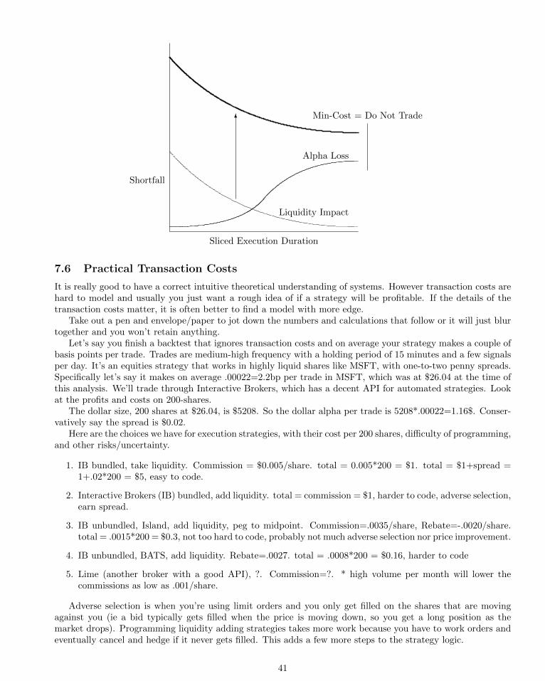
Shortfall
Sliced Execution Duration
Min-Cost = Do Not Trade
Alpha Loss
Liquidity Impact
6
7.6 Practical Transaction Costs
It is really good to have a correct intuitive theoretical understanding of systems. However transaction costs arehard to model and usually you just want a rough idea of if a strategy will be profitable. If the details of thetransaction costs matter, it is often better to find a model with more edge.
Take out a pen and envelope/paper to jot down the numbers and calculations that follow or it will just blurtogether and you won’t retain anything.
Let’s say you finish a backtest that ignores transaction costs and on average your strategy makes a couple ofbasis points per trade. Trades are medium-high frequency with a holding period of 15 minutes and a few signalsper day. It’s an equities strategy that works in highly liquid shares like MSFT, with one-to-two penny spreads.Specifically let’s say it makes on average .00022=2.2bp per trade in MSFT, which was at $26.04 at the time ofthis analysis. We’ll trade through Interactive Brokers, which has a decent API for automated strategies. Lookat the profits and costs on 200-shares.
The dollar size, 200 shares at $26.04, is $5208. So the dollar alpha per trade is 5208*.00022=1.16$. Conser-vatively say the spread is $0.02.
Here are the choices we have for execution strategies, with their cost per 200 shares, difficulty of programming,and other risks/uncertainty.
1. IB bundled, take liquidity. Commission = $0.005/share. total = 0.005*200 = $1. total = $1+spread =1+.02*200 = $5, easy to code.
2. Interactive Brokers (IB) bundled, add liquidity. total = commission = $1, harder to code, adverse selection,earn spread.
3. IB unbundled, Island, add liquidity, peg to midpoint. Commission=.0035/share, Rebate=-.0020/share.total = .0015*200 = $0.3, not too hard to code, probably not much adverse selection nor price improvement.
4. IB unbundled, BATS, add liquidity. Rebate=.0027. total = .0008*200 = $0.16, harder to code
5. Lime (another broker with a good API), ?. Commission=?. * high volume per month will lower thecommissions as low as .001/share.
Adverse selection is when you’re using limit orders and you only get filled on the shares that are movingagainst you (ie a bid typically gets filled when the price is moving down, so you get a long position as themarket drops). Programming liquidity adding strategies takes more work because you have to work orders andeventually cancel and hedge if it never gets filled. This adds a few more steps to the strategy logic.
41
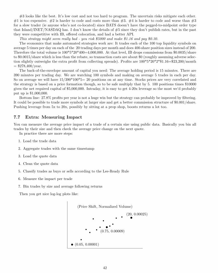
#3 looks like the best. It’s low cost and not too hard to program. The uncertain risks mitigate each other.#1 is too expensive. #2 is harder to code and costs more than #3. #4 is harder to code and worse than #3for a slow trader (ie anyone who’s not co-located) since BATS doesn’t have the pegged-to-midpoint order typethat Island/INET/NASDAQ has. I don’t know the details of #5 since they don’t publish rates, but in the pastthey were competitive with IB, offered colocation, and had a better API.
This strategy might seem really bad - you risk $5000 and make $1.16 and pay $0.30.The economics that make automated strategies work are: It trades each of the 100 top liquidity symbols on
average 5 times per day on each of the 20 trading days per month and does 400-share position sizes instead of 200.Therefore the total volume is 100*5*20*400=4,000,000. At that level, IB drops commissions from $0.0035/shareto $0.0015/share which is less than the rebate, so transaction costs are about $0 (roughly assuming adverse selec-tion slightly outweighs the extra profit from collecting spreads). Profits are 100*5*20*2*$1.16=$23,200/month= $278,400/year.
The back-of-the-envelope amount of capital you need: The average holding period is 15 minutes. There are390 minutes per trading day. We are watching 100 symbols and making on average 5 trades in each per day.So on average we will have 15/390*100*5= 20 positions on at any time. Stocks prices are very correlated andthe strategy is based on a price formation though, so to be safe multiply that by 5. 100 positions times $10000gives the net required capital of $5,000,000. Intraday, it is easy to get 4-20x leverage so the most we’d probablyput up is $1,000,000.
Bottom line: 27.8% profits per year is not a huge win but the strategy can probably be improved by filtering.It could be possible to trade more symbols at larger size and get a better commission structure of $0.001/share.Pushing leverage from 5x to 20x, possibly by sitting at a prop shop, boosts returns a lot too.
7.7 Extra: Measuring Impact
You can measure the average price impact of a trade of a certain size using public data. Basically you bin alltrades by their size and then check the average price change on the next quote.
In practice there are more steps:
1. Load the trade data
2. Aggregate trades with the same timestamp
3. Load the quote data
4. Clean the quote data
5. Classify trades as buys or sells according to the Lee-Ready Rule
6. Measure the impact per trade
7. Bin trades by size and average following returns
Then you get nice log-log plots like:
(Price Shift, Normalized Volume)
t (0.05, 0.00001)
rr r
rr r r t
(0.75, 0.00009)
r r r r t(20, 0.00025)
42
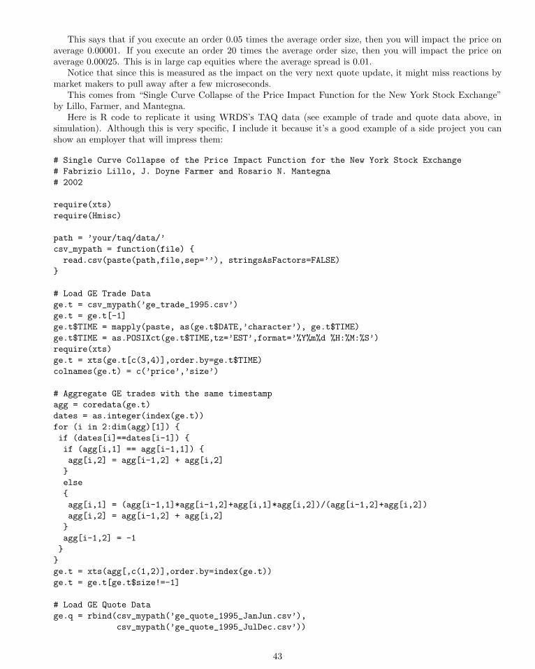
This says that if you execute an order 0.05 times the average order size, then you will impact the price onaverage 0.00001. If you execute an order 20 times the average order size, then you will impact the price onaverage 0.00025. This is in large cap equities where the average spread is 0.01.
Notice that since this is measured as the impact on the very next quote update, it might miss reactions bymarket makers to pull away after a few microseconds.
This comes from “Single Curve Collapse of the Price Impact Function for the New York Stock Exchange”by Lillo, Farmer, and Mantegna.
Here is R code to replicate it using WRDS’s TAQ data (see example of trade and quote data above, insimulation). Although this is very specific, I include it because it’s a good example of a side project you canshow an employer that will impress them:
# Single Curve Collapse of the Price Impact Function for the New York Stock Exchange
# Fabrizio Lillo, J. Doyne Farmer and Rosario N. Mantegna
# 2002
require(xts)
require(Hmisc)
path = ’your/taq/data/’
csv_mypath = function(file) {
read.csv(paste(path,file,sep=’’), stringsAsFactors=FALSE)
}
# Load GE Trade Data
ge.t = csv_mypath(’ge_trade_1995.csv’)
ge.t = ge.t[-1]
ge.t$TIME = mapply(paste, as(ge.t$DATE,’character’), ge.t$TIME)
ge.t$TIME = as.POSIXct(ge.t$TIME,tz=’EST’,format=’%Y%m%d %H:%M:%S’)
require(xts)
ge.t = xts(ge.t[c(3,4)],order.by=ge.t$TIME)
colnames(ge.t) = c(’price’,’size’)
# Aggregate GE trades with the same timestamp
agg = coredata(ge.t)
dates = as.integer(index(ge.t))
for (i in 2:dim(agg)[1]) {
if (dates[i]==dates[i-1]) {
if (agg[i,1] == agg[i-1,1]) {
agg[i,2] = agg[i-1,2] + agg[i,2]
}
else
{
agg[i,1] = (agg[i-1,1]*agg[i-1,2]+agg[i,1]*agg[i,2])/(agg[i-1,2]+agg[i,2])
agg[i,2] = agg[i-1,2] + agg[i,2]
}
agg[i-1,2] = -1
}
}
ge.t = xts(agg[,c(1,2)],order.by=index(ge.t))
ge.t = ge.t[ge.t$size!=-1]
# Load GE Quote Data
ge.q = rbind(csv_mypath(’ge_quote_1995_JanJun.csv’),
csv_mypath(’ge_quote_1995_JulDec.csv’))
43
ge.q = ge.q[-1]
ge.q$TIME = mapply(paste, as(ge.q$DATE,’character’), ge.q$TIME)
ge.q$TIME = as.POSIXct(ge.q$TIME,tz=’EST’,format=’%Y%m%d %H:%M:%S’)
ge.q = xts(ge.q[c(3,4)],order.by=ge.q$TIME)
colnames(ge.q) = c(’bid’,’ofr’)
# Clean GE Quote Data
ge.q = ge.q[!(ge.q$bid==0 | ge.q$ofr==0),] # Bid/Offer of 0 is a data error
ge = merge(ge.t, ge.q)
# Final Result: variable ’ge’ is an xts with NA’s showing trades / quotes
#ge.t = NULL
#ge.q = NULL
# Classify the direction of trades according to Lee-Ready (1991)
ge$mid = (ge$bid+ge$ofr)/2
ge$dir = matrix(NA,dim(ge)[1],1)
d = coredata(ge) # data.frame(coredata(ge)) is insanely slower
p1 = d[1,1]
d[1,6] = 1 # Assume the first trade was up
dir1 = d[1,6]
q1 = d[2,5]
for (i in 3:dim(d)[1])
{
p2 = d[i,1] # current price
if (!is.na(p2)) # Trade
{
# Quote Rule
if (p2 > q1)
{
d[i,6] = 1 # Direction
}
else if (p2 < q1)
{
d[i,6] = -1
}
else # p == midpoint
{
# Tick Rule
if (p2 > p1)
{
d[i,6] = 1
}
if (p2 < p1)
{
d[i,6] = -1
}
else # prices stayed the same
{
d[i,6] = dir1
}
}
p1 = p2
44
dir1 = d[i,6]
}
else # Quote
{
q1 = d[i,5] # Update most recent midpoint
}
}
# Measure impact per trade
d2 = cbind(d[,6],d[,2],log(d[,5]),matrix(NA,dim(d)[1],1))
colnames(d2) = c(’dir’,’size’,’logmid’,’impact’)
trade_i1 = 1
quote_i1 = 2
for (i2 in 3:dim(d2)[1])
{
dir_i2 = d2[i2,1]
if (!is.na(dir_i2)) # Trade
{
if (i2-trade_i1 == 1) # Following another a trade
{
d2[trade_i1,4] = 0 # \delta p = 0
}
trade_i1 = i2
}
else # Quote
{
if (i2-trade_i1 == 1) # Following a trade
{
d2[trade_i1,4] = d2[i2,3]-d2[quote_i1,3] # diff(logmids)
}
quote_i1 = i2
}
}
# Look only at buyer initiated trades
buy = d2[!is.na(d2[,4]) & d2[,1]==1,]
buy = buy[,c(2,4)]
buy[,1] = buy[,1]/mean(buy[,1])
require(Hmisc)
max_bins = 50
sizes = as.double(levels(cut2(buy[,1],g=max_bins,levels.mean=TRUE)))
buy[,1] = cut2(buy[,1],g=max_bins,levels.mean=TRUE)
ge_imp = aggregate(buy[,2], list(buy[,1]), mean)
plot(sizes,ge_imp[,2],log=’xy’,type=’o’,pch=15,ylab=’price shift’,
xlab=’normalized volume’,main=’GE’)
# Find how the price impact increases with volume
imp_fit = function(pow){summary(lm(ge_imp[,2] ~ I(sizes^pow)))$r.squared}
fits = sapply(seq(0,1,.01), imp_fit)
print(paste(’R^2 minimizing beta in volume^beta=impact:’,which.max(fits)/100))
print(’Difference is likely because of Lee-Ready flat trade/quote ambiguity’)
print(’and timestamp aggregation ambiguity.’)
print(’A huge number of trades were labeled as having 0 impact.’)
45
8 Programming
Computer Science is no more about computers than astronomy is about telescopes. –Dijkstra
This section contains standalone topics. Each is indirectly important for a quant researcher.
8.1 Design Patterns
In building trading systems, one notices patterns in how they are designing things. After you’ve built a couple,you start to see that they generally fall into certain classes based on time frequency and usage of data. Much ofthe infrastructure between systems feels the same, although getting the details right is always a little bit hardto do on the first attempt.
In computer science classes, one often encounters hard problems– designing efficient algorithms, writingsomething as concisely as possible, or solving a problem with only simple tools like bitwise operations. Howeverthere is another class of hard problems which one may unknowingly discuss in a class like “Software Engineering”but not directly encounter. Designing architectures is another category of hard problems which appear all thetime in real-world software engineering but are missed by classes because it’s infeasible to actually code alarge scale system in a semester and because it’s too hard for professors to grade vaguely specified projects.Design patterns are a way of coping with complexity and avoiding the tangles that can result from myopiccoding. Besides just guiding the architecture designer’s thought process, we can often construct re-usablemeta-frameworks and tools to speed future development.
Generally, the developer’s wisdom/learning curve follows these four steps, where you have to do each step3-5 times to move on to the next:
prototype→ full system→ intuit patterns→ extract frameworks
But let’s just jump ahead to the patterns.
Batch
Typically once per day or even less frequently, you run a script to download some historical data, run anotherscript to re-optimize a model based on that updated data, and finally output signals, typically to a file to beimported into the execution software and submitted, after a quick sanity check.
Let’s rewrite that as psuedocode to make it feel more actionable–
| Batch(Pattern)
1| download some historical data
2| re-optimize a model
3| if conditions met:
4| output buy signals
5| import into execution software
6| sanity check and submit
Batch systems are the most amenable to machine learning in terms of developer friendliness, but lowerfrequency systems unfortunately have less data to work with. For this kind of system, data is typically storedin a matrix where each row is a day of observations of all the interesting variables on a historical date.
Scheduled
I bring up schedule based systems second although they’re more challenging to design than event driven systemsbecause they are more intuitive based on human experience and more similar to TradeStation, OpenQuant, andother retail platforms which traders are probably familiar with. People are used to being driven by clocks ratherthan purely by unanticipatable external events and impulses.
Let’s go straight to code here, it’s clearer–
46
| Scheduled(Pattern)
1| turn on data stream
2| at time of day x:
3| calculate indicators
4| if conditions met:
5| submit order
One often designs according to this pattern when automating a strategy which is currently being tradeddiscretionarily. It might also arise in a case where you want to trade at the ‘close’, but to implement it youhave to check signals and place trades 10 minutes before, for example.
Event Driven
Event driven systems are the most powerful and flexible because they get closest to the raw data. Power andflexibility generally lead to more tedious code – think C++ vs. Excel. ‘High Frequency Trading’, as seen onTV, is generally event-driven.
The common patterns here are generally in seamlessly indexing by time and by message number, handlingstored data and indicators, and code efficiency. Execution and position tracking also become more complexwhen signals can change before executed trades are even confirmed.
In some sense though, these systems are the most fun to write because they don’t impose structural con-straints.
| Event(Pattern)
1| register data stream listener
2| turn on data stream
3| listener (on new data event):
4| calculate indicators
5| if conditions met:
6| submit order
Augmented Intelligence
GETCO, the world’s current top high frequency group, generally follows this pattern, and was the inspiration forits inclusion. Here the parts that humans are good at are delegated to humans, and the parts that a computer isgood at are delegated to the computer. Humans are good at analyzing world events, understanding what timeof day things will happen and what to watch out for, and developing a general feel for a certain day’s market.The computer is good at reacting on a microsecond basis and following parameters precisely and unemotionally.Basically a human is inserted as an intermediary between ‘the world’ and the automated trading system becausethere are a lot of common sense things a human knows about the world which turn out to be really hard to geta computer to understand.
squishy chaotic world→ human→ computer→ market
The human turns on or off the model whenever they feel like it. There are all kinds of models (I list somepossibilities here rather than previously because this is a relatively novel design pattern): A momentum modelthat is turned on a few minutes before earnings announcements and then turned off a few minutes after; a meanreversion algorithm that is activated on days that seem dull and don’t have any major news scheduled; a generalmarket making model that’s run all the time except in extreme circumstances; a triple-witching-day model; etc.
Some are designed to run for minutes, some all day. Some hold for milliseconds, some for hours. Asset classand breadth are similarly unrestricted.
Each model is unique, but they also have parameters, so they are optimizable to changing conditions.
| AugInt(Pattern)
1| have a feeling # human
2| set parameters # human
3| [other design pattern system here] # computer
47
8.2 Common Specialized Patterns
Session Management
This pattern, also called “fail-fast,” is used to make a system automatically recover from random disconnection.It is mandated by many of the main exchange’s DMA protocols (FIX, NASDAQ OUCH).
for(;;) {
connect()
while(isConnected()) {
doAutomatedTrading()
}
sleep(1)
print(attempting to connect!!)
}
This wraps the entire strategy and makes it more robust to network errors.
Finite State Machine
FSMs are used to locally track the state of objects on a remote server. This is good for handling multi-step asyncronous request-response—error—cancel logic chains. FSMs are also easy to visualize. For example,submitting a limit order to buy and working it at the best bid until it is executed or fails is a multi-step branchingprocess. The states are: { Submitted, Canceled, Accepted, Filled, Partially Filled }. Transitions occur whenthe bid changes, the exchange rejects the order, an execution report arrives, or a broker status message arrives.
There is not a one-size fits all FSM implementation. Sometimes you will want all the state transition logiccentralized in a switch-case statement, sometimes you will want it in each state. Sometimes states will be assimple as an enum, sometimes they will be full-fledged objects with multiple instance variables. Sometimes youwill want states to share information via global variables, sometimes via arguments. FSMs which are workingorders could be nested within an overall strategy FSM.
The FSM is a powerful tool for making complicated logic consistent and simpler to understand.
8.3 APIs
The API is the code library that lets your system send commands to the broker. Point and click trading GUIsthat most traders place trades through are built on top of an API. Some brokers allow you to access the API.This allows third party companies to build specialized GUIs and quants to build automated trading systems.The API code library handles opening a socket connection to the broker’s server, reading and writing to thesocket, constructing and parsing messages based on the brokers protocol, and passing data up to and down fromhigher level API calls. The API library is language specific, usually C++, Java, or Excel.
An API generally serves two concerns, data and execution.In each part there will be functions to login, place requests, and logout, and callbacks to receive data.We’ll compare a couple of designs closely based on actual brokers’ APIs (the names are changed, and the
code is made language agnostic although strongly typed). Let’s call these brokers A, B, and C. To connect wehave the following function signatures:
void connectA(string host_ip_address, int port, int connection_id)
int connectB(string host, string user, string pswrd, boolean cancel_on_disconnect)
/* connectC does not exist - GUI based */
Broker A requires the user to have another application logged-in and running in the background. So connectAdoes not require a username and password. Also, it returns void since Broker A’s API is totally asynchronous.You have to listen to callbacks to determine whether you are actually connected. It also requires a uniqueconnection id per session. There is a special case– connection id 0 is for the included GUI and receives callbacks
48
from all connections. The purpose and recommendations for what id number to use are not clearly explainedin the documentation.
connectB is better. The function to connect and login is a good candidate to make synchronous since it isnot speed-sensitive, is only called once, nothing else needs to be run while you are waiting for it, and loggingin does not produce a queue of messages coming over the network. It returns an int which is non-zero if thelogin was sucessful, just like the UNIX convention. It also has a convenient option to try to cancel all trades,reducing risk, if there is a network outage.
connectC does not exist since broker C requires you to have a lightweight GUI/console application runningin the background. Although not automated, this is ok since you typically only log in once per day or less.
connectA is the worst and connectB is the best. An API is a balance between flexibility and ease of use forcustomers’ typical use case. The common use case is having a fully automated system connecting once per day.C is not fully automated, A ignores the fact that you only connect once per day.
Now let’s look at requesting data:
void subscribeA(int request_id, Contract contract,
string tick_type_list, boolean snapshot)
/* Contract is data object with constructor and 16 fields, some of which are
optional, some of which have easy to misspell names, most of which are
only required under certain complicated conditions.
tick_type is a string of comma-separated ints corresponding to data such
as BID_SIZE, LOW_52_WEEK, INDEX_FUTURE_PREMIUM, and AUCTION_IMBALANCE
snapshot is a boolean saying whether you just want one point or an ongoing
subscription to the feed */
int subscribeB(string quote_source, string[] symbols)
int subscribeAllB(string quote_source)
/* subscribeC does not exist - automatically subscribed to all symbols in
symbol.list file on startup */
Broker A fails again, this time miserably. As consolation, they were historically one of the first to offer an API,and APIs are hard to change without breaking client applications. They also support more types of securities,more exchanges, more account types, and more countries so they require a lot more details to unambiguouslyspecify a contract. However they should have a more consistent contract naming scheme, eliminate special casesand conditionally required fields, and lean more heavily on the compiler’s type-checker to enforce proper usage.
connectB is great. Since broker B only offers access to US equities, it is easy to name contracts. It returnsan int to tell whether the request was acknowledged by the broker’s server. A separate function is offered torequest all contracts rather than creating a huge array of all the contracts’ symbols.
Broker C requires clients to be colocated in their data center at the exchange. Since the computer must beextremely special purpose, they can make it so that as soon as it connects, it automatically reads the config fileand requests the data without explicitly calling any function.
Broker A is bad, B is developer, user, and prototyping friendly, and C is the most barebones but effective.Like logging in, requesting data is a good candidate to make synchronized or automatic since it typically isn’tbeing called often.
Typically a trading system is designed as a set of logical rules within a data callback function, which placestrades if the new data point matches the right conditions. So the data callback is very important. Let’s look ata few side-by-side:
void priceA(int request_id, int field, double price, boolean can_auto_execute)
/*
field :=
Value Description
1 bid
2 ask
49
4 last
6 high
7 low
9 close
*/
void sizeA(int request_id, int field, int size)
/*
field :=
Value Description
0 bid
3 ask
5 last
8 volume
*/
void genericA(int request_id, int tick_type, double value)
void stringA(int request_id, int tick_type, string value)
void ask_quoteB(string symbol, long quote_server_id, int size, double price,
string mmid, string quote_source, long timestamp)
void bid_quoteB(string symbol, long quote_server_id, int size, double price,
string mmid, string quote_source, long timestamp)
void tradeB(string symbol, int size, double price, int total_volume,
string exchange_id, string quote_source, long timestamp,
string trade_type)
void quote_eventC(string symbol, long event_type, long bid_price, long bid_size,
long ask_price, int ask_size, long event_time, char venue)
/*
event_type :=
Value Description
0 NO_INSIDE_CHANGE
1 INSIDE_BID_PRICE_CHANGE_ONLY
2 INSIDE_BID_SIZE_CHANGE_ONLY
3 INSIDE_BID_PRICE_AND_SIZE_CHANGE
4 INSIDE_ASK_PRICE_CHANGE_ONLY
5 INSIDE_ASK_SIZE_CHANGE_ONLY
6 INSIDE_ASK_PRICE_AND_SIZE_CHANGE
}
venue :=
Value Description
I Nasdaq - INET
A NYSE ARCA
T BATS Exchange
G Direct Edge - EDGX
*/
Broker A is again the worst. They split the data across multiple overlapping callbacks. Tick size, price, andstring callbacks will be triggered with each new data point. The user has to match up the size to the price. Thedocumentation does not say whether the price or size should arrive first, so it is unclear which one you shouldhave trigger the trading logic. It also does not say whether every single data point triggers both a size and pricecallback. Splitting them up seems to imply they might not always be called at the same time, but as far as Iknow they are. stringA is redundant with the first two. genericA is used for special data as explained above.You also have to store and use the original request id number to figure out which contract the data refers to.
50
B and C are both good.Now that we have looked at logging in and data, let’s look at placing orders and receiving execution reports.
void orderA(int order_id, Contract contract, Order order)
/* Contract is same as in subscribeA(), Order is a data class with 62 fields */
long orderB(string symbol, int quantity, double price, string type, string route,
string properties)
/* where type := BUY, BUY_COVER, SELL, and SHORT,
properties is a key=value comma delimited string supporting algos, specific
routing, and special order types specific to certain exchanges
return value is the unique order_id for cancellation and modification */
long orderC(long * order_id, string symbol, char side, long quantity, long price,
char route, long tif, char display, long display_quantity,
long discretion_offset, char route_strategy, char algo, double account)
/*
return value :=
0 NO ERROR
2 ERROR BAD SYMBOL
3 ERROR BAD PRICE
4 ERROR GATEWAY CONNECTION DOWN
5 ERROR TOO MANY OPEN ORDERS ON THIS SYMBOL
6 ERROR CANNOT CREATE THIS ORDER
7 ERROR BAD ORDER TYPE
13 ERROR BAD ACCOUNT
*/
All three are close to equal for sending orders.A is again slightly worse though. Users have to furnish order id numbers, and it is not well specified what
should happen when you overflow int. It also has 4 different id’s and it’s not clear which are required, whichmust be unique, and which must be the same. The Order object itself has a “permanent”, “client” and “order”id. The function call specifies an order id. It’s not clear why the client id can’t be inferred from the currentsession settings, nor whether the permanent id matters. B and C assign the order id for you and then return it.
A again suffers from trying to pack functionality for all types of securities, exchanges, and clients into asingle function call.
Ideally, all APIs could be improved to use the type checker to catch errors at compile-time, rather thanruntime. Broker C made a half-hearted attempt to catch errors by having an error-status return type. How-ever multiple of these errors could be caught at compile time instead if runtime. Debugging event-driven,asynchronous systems is challenging so compile time checks are a huge benefit.
Placing orders with an API is more complicated than it looks, since after placing it a number of thingscan happen. The order can be filled, partially filled, rejected by the broker or exchange, sit on the book, thenetwork can become congested, or your program can crash. You will be tempted to prematurely optimize howyou track your current position. If you are just trading one contract you might have an int currentPosition
variable that is negative when you are short and positive when long. This is the wrong approach. Unless yoursystem is extremely simple and only uses market orders, you should not do this. Keep an (orderId, OpenOrder)hashmap of all orders. When one is filled or cancelled, remove it. When one is partially filled, deduct the size.Create seperate methods to calculate your total size in each contract. This is one of the best places to useencapsulation.
Finally, let’s look at execution notifications (all return void):
openA(int order_id, Contract contract, Order order, OrderState state)
statusA(int order_id, string status, int filled, int remaining,
double avg_price, int perm_id, int parent_id,
double last_price, int client_id, string locating)
51
update_portfolioA(Contract contract, int position, double market_price,
double mkt_value, double avg_cost, double unrealized_pnl,
double realized_pnl, string account_name)
executionA(int reqId, Contract contract, Execution execution)
statusB(int status_type, long order_id, string symbol, double quantity,
double price, string trade_type, string route, long timestamp,
string reason)
cancelrejectB(long order_id, string reason_text, int reason)
executionB(long order_id, string exec_id, string symbol, double quantity,
double price, string trade_type, string route, long timestamp,
string properties)
position_changeB(string symbol, double position)
openC(long order_id, string symbol, double account, long timestamp)
cancelC(long order_id, string symbol, double account, long timestamp)
rejectC(long order_id, string symbol, double account, long timestamp, char reason)
cancelrejectC(long order_id, string symbol, double account, long timestamp,
char reason)
executionC(long order_id, string symbol, char side, long quantity, long price,
long exec_id, string contra, char liquidity_fee, char exchange,
double account , long ecn_fee, long sec_fee, long timestamp)
Clearly the most functions are dedicated to execution reporting because there are multiple outcomes tosubmitting an order.
Unfortunately broker A again tried to cram all the functionality into one method, statusA. It’s not entirelyobvious from the signature, but the status field has the possible value “Submitted”, which supersedes openA;“Filled”, which supersedes part of executionA; “Cancelled” and “Inactive”. This is very confusing for beginningdevelopers because they wonder why 4 methods do overlapping things. So the beginner thinks that they areusing them wrong because no company would release such a poor design. Unfortunately, broker A did.
Again unfortunate is that A does not give any details about why an order might be cancelled, unlike brokersB and C do.
Broker A also does not provide detailed information about execution costs, liquidity rebates, and other fees.Broker B has a little bit of overlapping functionality in the position changeB callback since one could
reconstruct their position based on a series of execution reports. But many trading systems do not work limitorders, and simplicity is preferred to flexibility. The simple position changeB function, with just two arguments,satisfies this need without causing confusion.
B and C are again similar and both well-designed.In summary we can see broker A’s design flaws and B and C’s successes. You can see how they accomodate
users with difference levels of sophistication, running on different platforms, trading different contracts. BrokerB was slightly easier to use with a synchronized login and simple position change callback. C assumed userswould be colocated and had more development skill.
We have ignored many other functionality including requesting account information, other types of data,and session error handling, but the successes and failures are very similar across all parts of each brokers API. Ishould also mention that broker A’s documentation is far worse than B and C’s, making their flawed API evenmore frustrating.
8.4 Programming Language
“What programming language is the best for trading systems?” is a fairly common question on web forums.It’s hard to answer because it’s sort of like the question, “do you know you’re ugly?” – “yes” and “no” areimplied as the only possible answers, but you don’t want to say either since then you’re admitting you’re ugly.The implied answer set is all inapplicable. In this case, if you have to ask, then you probably have no idea what
52
you’re doing. You need to go through a formal computer science degree program at a college to have any hopeof designing a trading system from scratch.
Domain specific languages such as Tradestation’s EasyLanguage, Algodeal’s Market Runner, MetaTrader’sMQL5, and NinjaTrader’s Ninjascript are the best option for people with no programming experience. Forsimple, technical-indicator strategies that trade single assets independently and don’t use any regression andaren’t adaptive, a DSL is definitely the way to go even for experienced programmers. They typically handle allthe details of managing data, writing a backtester, calculating indicators, running things at the right time ofday, and so on.
One step up from this are Excel-based systems. Many brokers have an Excel API. Excel is easy to debugand tweak since all the numbers are always editable and visible. It is also the most sophisticated programmableenvironment that non-programmers are comfortable using. Computer scientists who are bothered by this shouldtake care not to think of everything as a nail just because you are skilled in the use of hammers. Manygood proprietary trading shops use Excel-based models for slower strategies such as fixed income trading. Forstrategies that are simple but don’t fit in the framework of the available DSLs or strategies which benefit fromhuman supervision and intervention, Excel is a good choice.
Moving beyond Excel, typically the choice of which langauge to use is most constrained by the APIs yourbroker offers. In practice all mainstream languages are pretty much equivalent (Java, C++, .NET, maybePython or a LISP). Most skilled programmers are indifferent between languages (except hipster programmerswho program just for its own sake). By skilled programmer I mean you are either majoring in computer scienceand have a good GPA or you work as a developer. If this is not you, be honest with yourself and don’t wastetime in this section because the complexity of a trading system will probably end up being too much. Howeverif you are a programmer, the best language to pick is the native one for your broker’s API.
The final step up is a developer working at a trading firm. You can use any language since your firm has theresources to develop to an exchange’s protocol rather than using an API. Most high frequency firms use C++or Java.
In summary:
Programming skill Language to useVery little Domain specific languageUse Excel or Matlab day-to-day Excel or domain specific languageProfessional developer Same as broker’s API (Java, C++, .NET)Developer at trading firm Any
8.5 OS and Hardware Platform
Unfortunately this section has to be negative like the previous one. Choice of operating system and hardwareplatform seems to be the most tempting place for premature optimization. It’s to the point that people won’teven create a single trading system because they are so busy debating the benefits of Linux and cloud hosting.Just go write version 1 and run it every day for a full week on whatever desktop or laptop you have if thisdescribes you. So much has been written about the topic of trader psychology, I think someone should writeabout quant trader psychology.
Use the operating system that your broker’s API targets – if they have Visual C++ project files or a .NETAPI then use Windows and if they use Linux system calls, use Linux. Don’t spend time trying to port it becausethen you will have to port every new version as well. The operating system imposes almost no new constraintson what you can do. There are high frequency trading firms using Windows.
There are three options for hardware platform: home computer, cloud host, or colocation.As I write this in Mar 2011, cloud hosting is getting to be about as easy to run a trading system on as a
computer at home. It has the advantages of 24/7 uptime, low costs, typically excellent network connections,choice of the operating system, and complete dedication to trading rather than shared with other programs.However if you have a good internet connection at home and an extra computer, then either one is fine.
Colocation has two benefits and a lot of costs. The benefits are low latency, which can make or break certaintypes of strategies, and access to tick data. Most data providers won’t deliver high-bandwidth tick data over theinternet. If you have a strategy idea that, say, requires counting the number of trades that were buyer initiatedvs seller initiated over the past minute, you will need tick data. The cheapest colocation provider I’m aware
53

of (Lime Brokerage) costs 400 dollars per month per server and you need to meet high but not unreasonabletrading volume minimums. Another cost is the hassle and experience required to buy a server, mail it to thecolocation facility, log in remotely, etc. Colocation facilities do have on-site staff so you can call and have themmake hardware changes remotely.
There are two options within colocation – placing trades through a broker and connecting directly to anexchange. The latter option costs tens of thousands of dollars per month or more and requires registering withthe SEC as a broker-dealer.
Here are rough latency numbers and a summary:
Platform Latency Upgrade to next ifHome PC 100ms No extra computer, patchy internetCloud 10ms Latency-sensitive, need tick dataColo with broker 1ms You are the CEO of a HFT prop shopColo with exchange 500ms
9 Fix-it Game
Description
Fix-it is a card game that is a lot like real trading. The job of a trader is to estimate the true value of sharesand buy or sell them to make a profit when the prices reach their true value. In this game, the average valueof the cards on the table represent the true value of some share. Some cards are known only to one person,some are known to everyone. The players are traders. They try to estimate the average value of the cards thathave been dealt (including hidden ones) and trade with other players so that they make a profit if that estimateis correct. One can also trade profitably by tricking other players, making a market, by luck, guessing whatcards other players have, or in other ways. The cards that are shown to everyone are revealed slowly so thatinformation is revealed gradually. After all the shared cards have been revealed and trading stops, players showtheir hidden cards, and players’ final positions are liquidated at the true price.
Supplies
A deck of cards, one sheet of paper, and a pen.
Setup
Every player is dealt 1 card, and there are 3 cards face down on the table. The cards are given numerical valuesfrom 1-13 for Ace to King.
Goal
Capture the largest positive spread between the average of all the cards in play and the trades in your book.
Accounting
One player must account for all trades. The other players will check what is written down as well. The tradeblotter has a column for each player and a row for each transaction. In a row, the price of the share that wastransacted is recorded as positive in the sellers column and negative in the buyers column.
All shares are liquidated at the true value once trading ends and the true value is revealed. To figure out aplayer’s inventory, add the count of negative numbers (shares bought) in their column and subtract the countof positive numbers (shares sold). The net liquidation value is the inventory times the true price. To see whomade the most profit, add up their column and their inventory liquidation value. The winner is the person withthe most money.
54

Rules
There are three rounds. A round ends before the next shared card is flipped up. The game ends when the thirdshared card is flipped up and everyone has finished trading.
Each player can buy or sell single shares to other players. Some player, call her A, engages the transactionby pinging the market. They ask if anyone is interested in buying (selling) at a specific price X. If some player,B, believes that price is good, then she will agree to buy (sell) one share at X. The accountant then recordsthe trade as a new row with +X under player A and −X under player B.
All players trade with each other until everyone agrees to finish the round. this process can be very chaotic,as there is no process for bidding.
Remember: no one knows what the true value of the sum of all the cards in play are until the end of thegame, so it is purely speculative.
Once no more trades are being done and everyone agrees to finish the round, it ends. Then another one ofthe 3 face down cards is flipped up and the next round of trading begins. Players trade again until they arefinished.
This repeats two more times, until all 3 cards on the table are face up. After this last trading round is over,all players show their cards, and the true price is calculated. The player with the most money after liquiditinginventory wins.
To liquidate a player’s inventory: (1) add up the number (not the value) of − trades in a player’s columnand (2) subtract the number of + trades, to get the total inventory, and then (3) multiply this by the finalprice, to get the value of inventory. Then (4) add up the total value of the trades in the players column and (5)add this to the value of the inventory to get the player’s total money.
It is easy to calculate the average value of the deck, which makes a good first estimate of the true value.After trading, players should begin to understand what other players cards are. If people are buying a lot orselling a lot, that is a useful piece of market information as to what card they may have.
10 Pit Trading Game
The Pit Trading Simulation is run semi-annually at UC Berkeley. The organizer invents a “security” to trade.The security is usually something like a car or bottle of wine. The organizer makes up a series of newsannouncements about the security, such as “the car came out in 2004,” “the car was bought used,” “the car hasspinning rims,” etc which dramatically change the price of the security throughout the game. Participants tradeon the price of the car. At the end of the game, the organizer announces the true price and everyone coverstheir inventory at that price. Whoever made the most money wins. The following page is the rules provided tocontestants.
55

Pit Trading Simulation The objective of this simulation is to simulate the trading environment of a Pit, suchas the S&P Futures Pit in Chicago. However we trade a common product instead of a financial asset like theS&P Futures.
You are split up into teams of 4 – 2 market makers and 2 traders. The job of the market makers is to writethe up-to-date Bid and Offer prices that the team wants to show on the board. When you want to changethe bid/offer price, you simply write a new one and then cross out the old one. The job of the traders is towalk around the Pit and trade with the other teams market makers. You cannot trade against your own teamsmarket makers or with other groups traders.
You have slips like this to record trades:
M. M. ID Tr. ID (B)uy/(S)ell Price
Here are a few examples of recording trades: You are Trader B of Team 2. Team 5 has a Bid of 10 and anOffer of 15. You like their offer, and buy at 15. Team 5s market maker B records that you have purchased onecontract at 15. Fill out a slip like this (the market maker fills in the M. M. ID field):
M. M. ID Tr. ID (B)uy/(S)ell Price5B 2B B 15
The market maker fills out a similar slip showing Sell instead of Buy and has you fill in Tr. ID:
M. M. ID Tr. ID (B)uy/(S)ell Price5B 2B S 15
You are Trader B of Team 1. Team 4 has a Bid of 4 and an Offer of 9. You like their bid, and sell at 4.Market maker A records the trade. Fill out a slip like this and have M. M. A write their ID:
M. M. ID Tr. ID (B)uy/(S)ell Price4A 1B S 4
The market maker fills out a similar slip showing Sell instead of Buy and has you fill in Tr. ID:
M. M. ID Tr. ID (B)uy/(S)ell Price4A 1B B 4
Remember, you buy at the offer and sell at the bid.A few other important rules: Traders: You cannot make more than one trade at once no matter how excited
you are at a teams Bid/Offer. Finish filling out the slips before trading again. Market Makers: Even if you arecurrently filling out a slip, if your bid or offer is hit, you must honor that price. This is why it is very helpfulto have two market makers per team, giving one the job of signing slips, and the other the job of updatingbid/offers. Only once a new price is written does the old price no longer count it does not matter if you crossit out.
NOTE: PLEASE WRITE CLEARLY! IF YOU CALCULATE YOUR PROFIT INCORRECTLY AT THEEND, YOU WILL BE FINED THE AMOUNT THAT YOU EXCEED THE AUDITED PROFIT.
First we will run a simulation that will run for only a few minutes where everyone can get somewhat familiarwith what they are doing. Then, we will run the full simulation which should last a bit longer. Every fewminutes, I will release news on the product being traded. It is your job as traders and market makers to digestthe news as it comes out, and act accordingly. Good luck.

11 Recommended Media
In conclusion, here’s what I recommend next:Books:
1. Active Portfolio Management, Grinold and Kahn
2. Trading and Exchanges, Larry Harris
3. A Perspective on Quantitative Finance: Models for Beating the Market, Quantitative FinanceReview 2003, Ed Thorp
4. Marco Dion: A researcher reveals a couple of his favorite strategies and why they tend towork so well, Active Trader Magazine Interview
5. Reminiscences of a Stock Operator, Jesse Livermore
6. Elements of Statistical Learning Theory, Hastie, Tibshirani
Videos:
1. Youtube: If You Had Everything Computationally Where Would You Put it, Financially?,GoogleTechTalks, David Leinweber
2. Matlab Webinars: Algorithmic Trading, Aly Kassam
3. Hulu: Wall St Warriors Seasons 1 and 2
57