matthias j. ehrhardt and lukas f. lang
TRANSCRIPT

Inverse Problems
Matthias J. Ehrhardt and Lukas F. Lang
Last updated on: March 9, 2018
Lecture NotesLent Term 2017/2018
This work is licensed under a Creative Commons “Attribution-NonCommercial-ShareAlike 3.0 Unported” license.

2

Contents
1 Introduction to inverse problems 71.1 Examples . . . . . . . . . . . . . . . . . . . . . . . . . . . . . . . . . . . . . 8
1.1.1 Matrix inversion . . . . . . . . . . . . . . . . . . . . . . . . . . . . . 81.1.2 Differentiation . . . . . . . . . . . . . . . . . . . . . . . . . . . . . . 91.1.3 Deconvolution . . . . . . . . . . . . . . . . . . . . . . . . . . . . . . . 91.1.4 Tomography . . . . . . . . . . . . . . . . . . . . . . . . . . . . . . . . 10
2 Linear inverse problems 132.1 Generalised solutions . . . . . . . . . . . . . . . . . . . . . . . . . . . . . . . 152.2 Generalised inverse . . . . . . . . . . . . . . . . . . . . . . . . . . . . . . . . 182.3 Compact operators . . . . . . . . . . . . . . . . . . . . . . . . . . . . . . . . 212.4 Singular value decomposition of compact operators . . . . . . . . . . . . . . 22
3 Regularisation 273.1 Parameter-choice strategies . . . . . . . . . . . . . . . . . . . . . . . . . . . 30
3.1.1 A-priori parameter choice rules . . . . . . . . . . . . . . . . . . . . . 313.1.2 A-posteriori parameter choice rules . . . . . . . . . . . . . . . . . . . 323.1.3 Heuristic parameter choice rules . . . . . . . . . . . . . . . . . . . . . 33
3.2 Spectral regularisation methods . . . . . . . . . . . . . . . . . . . . . . . . . 343.2.1 Convergence rates . . . . . . . . . . . . . . . . . . . . . . . . . . . . 363.2.2 Truncated singular value decomposition . . . . . . . . . . . . . . . . 373.2.3 Tikhonov regularisation . . . . . . . . . . . . . . . . . . . . . . . . . 373.2.4 Source-conditions . . . . . . . . . . . . . . . . . . . . . . . . . . . . . 373.2.5 Asymptotic regularisation . . . . . . . . . . . . . . . . . . . . . . . . 393.2.6 Landweber iteration . . . . . . . . . . . . . . . . . . . . . . . . . . . 40
3.3 Tikhonov regularisation revisited . . . . . . . . . . . . . . . . . . . . . . . . 44
4 Variational regularisation 474.1 Variational methods . . . . . . . . . . . . . . . . . . . . . . . . . . . . . . . 50
4.1.1 Background . . . . . . . . . . . . . . . . . . . . . . . . . . . . . . . . 504.1.2 Minimisers . . . . . . . . . . . . . . . . . . . . . . . . . . . . . . . . 554.1.3 Existence . . . . . . . . . . . . . . . . . . . . . . . . . . . . . . . . . 554.1.4 Uniqueness . . . . . . . . . . . . . . . . . . . . . . . . . . . . . . . . 58
4.2 Well-posedness and regularisation properties . . . . . . . . . . . . . . . . . . 594.2.1 Existence and uniqueness . . . . . . . . . . . . . . . . . . . . . . . . 594.2.2 Continuity . . . . . . . . . . . . . . . . . . . . . . . . . . . . . . . . . 644.2.3 Convergent regularisation . . . . . . . . . . . . . . . . . . . . . . . . 664.2.4 Convergence rates . . . . . . . . . . . . . . . . . . . . . . . . . . . . 69
3

4 CONTENTS
5 Numerical Solutions 715.1 More on derivatives in Banach spaces . . . . . . . . . . . . . . . . . . . . . . 715.2 Minimization problems . . . . . . . . . . . . . . . . . . . . . . . . . . . . . . 73
5.2.1 Gradient Descent . . . . . . . . . . . . . . . . . . . . . . . . . . . . . 73
CONTENTS 5
These lecture notes are based on the course “Inverse Problems in Imaging”, which washeld by Matthias J. Ehrhardt and Martin Benning in Michelmas term 2016 at the Universityof Cambridge.1 Complementary material can be found in the following books and lecturenotes:
(a) Heinz Werner Engl, Martin Hanke, and Andreas Neubauer. Regularization of InverseProblems. Vol. 375. Springer Science & Business Media, 1996.
(b) Martin Burger. Inverse Problems. Lecture notes winter 2007/2008.
http://www.math.uni-muenster.de/num/Vorlesungen/IP_WS07/skript.pdf
(c) Andreas Kirsch. An Introduction to the Mathematical Theory of Inverse Problems.Vol. 120. Springer Science & Business Media, 1996.
(d) Kazufumi Ito and Bangti Jin. Inverse Problems: Tikhonov Theory and Algorithms.World Scientific, 2014.
(e) Per Christian Hansen. Discrete Inverse Problems: Insight and Algorithms. Funda-mentals of Algorithms, SIAM Philadelphia, 2010.
(f) Otmar Scherzer, Markus Grasmair, Harald Grossauer, Markus Haltmeier and FrankLenzen. Variational Methods in Imaging. Applied Mathematical Sciences, SpringerNew York, 2008.
(g) Jennifer L. Mueller and Samuli Siltanen. Linear and Nonlinear Inverse Problemswith Practical Applications. Vol. 10. SIAM, 2012.
(h) Andreas Rieder. Keine Probleme mit Inversen Problemen (in German). Vieweg+TeubnerVerlag. 2003.
(i) Christian Clason. Inverse Probleme (in German), Lecture notes winter term 2016/2017
https://www.uni-due.de/~adf040p/skripte/InverseSkript16.pdf
These lecture notes are under constant redevelopment and might contain typos orerrors. We very much appreciate the finding and reporting of those (to [email protected] to [email protected]). Thanks!
1http://www.damtp.cam.ac.uk/research/cia/teaching/2016inverseproblems.html

6 CONTENTS

Chapter 1
Introduction to inverse problems
Solving an inverse problem is the task of computing an unknown quantity from observed(and potentially noisy) measurements. Typically, these two are related via a forwardmodel. Inverse problems appear in a variety of fields such as physics, biology, medicine,engineering, and finance, and include—for instance—tomography (e.g. computed tomog-raphy (CT)), machine learning, computer vision, and image processing. In this lecturecourse we address mathematical aspects of linear inverse problems that are needed to findstable and meaningful solutions.
The main focus of this lecture is the solution of the operator equation
Ku = f (1.1)
with given measurement data f for the unknown quantity u. Here, K : U → V denotes alinear operator that maps from a space U to a space V. We will restrict ourselves to thestudy of bounded linear operators between Hilbert spaces.
Computing a solution to (1.1) is typically not straightforward in most relevant appli-cations for three basic reasons:
• a solution might not exist,
• if it exists it might not be unique,
• small errors (such as noise) in the measurements get heavily amplified.
The latter has the potential to render solutions useless without proper treatment.In the sense of Hadamard the problem (1.1) is called well-posed if
• for all input data there exists a solution to the problem, i.e. for all f ∈ V there existsa u ∈ U with Ku = f .
• for all input data this solution is unique, i.e. u 6= v implies Kv 6= f .
• the solution of the problem depends continuously on the input datum, i.e. for allukk∈N with Kuk → f implies uk → u.
If any of these conditions is violated, problem (1.1) is called ill-posed. In the following wewill see that many relevant inverse problems are ill-posed.1
1In fact, the name ill-posed problems may be a more suitable name for this lecture, as the real challengeis to deal with the ill-posedness of these problems. However, the name inverse problems became morewidely accepted.
7
8 1.1. EXAMPLES
1.1 Examples
In the following we are going to present various examples of inverse problems and highlightthe challenges in solving them.
1.1.1 Matrix inversion
One of the most simple (class of) inverse problems that arises from (numerical) linearalgebra is the solution of linear systems. These can be written in the form of (1.1) withu ∈ Rn and f ∈ Rn being n-dimensional vectors with real entries and K ∈ Rn×n being amatrix with real entries. We further assume K to be symmetric, positive definite.
We know from the spectral theory of symmetric matrices that there exist eigenvaluesλ1 ≥ λ2 ≥ . . . ≥ λn > 0 and corresponding (orthonormal) eigenvectors kj ∈ Rn forj ∈ 1, . . . , n such that K can be written as
K =n∑j=1
λjkjk>j . (1.2)
It is well known from numerical linear algebra that the condition number κ = λ1/λn is ameasure of how stable (1.1) can be solved, which we will illustrate in the following.
We assume that we measure f δ instead of f , with ‖f − f δ‖2 ≤ δ‖K‖ = δλ1, where‖ · ‖2 denotes the Euclidean norm of Rn and ‖K‖ the operator norm of K (which equalsthe largest eigenvalue of K). Then, if we further denote with uδ the solution of Kuδ = f δ,the difference between uδ and the solution u to (1.1) is
u− uδ =
n∑j=1
λ−1j kjk
>j (f − f δ).
Therefore, we can estimate
‖u− uδ‖22 =n∑j=1
λ−2j ‖kj‖22︸ ︷︷ ︸
=1
|k>j (f − f δ)|2 ≤ λ−2n ‖f − f δ‖22,
due to the orthonormality of eigenvectors, the Cauchy-Schwarz inequality, and λn ≤ λj .Thus, taking square roots on both sides yields the estimate
‖u− uδ‖2 ≤ λ−1n ‖f − f δ‖2 ≤ κδ.
Hence, we observe that in the worst case an error δ in the data y is amplified by the con-dition number κ of the matrix K. A matrix with large κ is therefore called ill-conditioned.We want to demonstrate the effect of this error amplification with a small example.
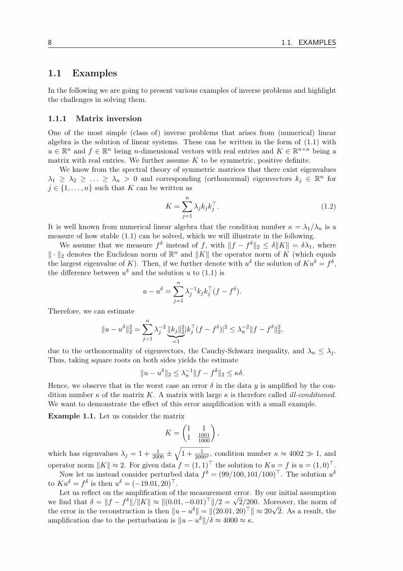
Example 1.1. Let us consider the matrix
K =
(1 11 1001
1000
),
which has eigenvalues λj = 1 + 12000 ±
√1 + 1
20002, condition number κ ≈ 4002 1, and
operator norm ‖K‖ ≈ 2. For given data f = (1, 1)> the solution to Ku = f is u = (1, 0)>.Now let us instead consider perturbed data f δ = (99/100, 101/100)>. The solution uδ
to Kuδ = f δ is then uδ = (−19.01, 20)>.Let us reflect on the amplification of the measurement error. By our initial assumption
we find that δ = ‖f − f δ‖/‖K‖ ≈ ‖(0.01,−0.01)>‖/2 =√
2/200. Moreover, the norm ofthe error in the reconstruction is then ‖u− uδ‖ = ‖(20.01, 20)>‖ ≈ 20
√2. As a result, the
amplification due to the perturbation is ‖u− uδ‖/δ ≈ 4000 ≈ κ.

CHAPTER 1. INTRODUCTION TO INVERSE PROBLEMS 9
1.1.2 Differentiation
Another classic inverse problem is differentiation of data. Assume we are given a functionf with f(0) = 0 for which we want to compute u = f ′. For f sufficiently smooth, theseconditions are satisfied if and only if u and f satisfy the operator equation
f(y) =
∫ y
0u(x) dx,
which can be written as the operator equation Ku = f with the linear operator (K·)(y) :=∫ y0 ·(x) dx.
As before, we assume that instead of f we measure a perturbed version f δ = f+nδ withf ∈ C1([0, 1]) and noise nδ ∈ L∞([0, 1]). It is obvious that the derivative u exists if thenoise nδ is differentiable. However, even in the (unrealistic) case that nδ is differentiable,the error in the derivative can become arbitrarily large as we will see.
Consider a sequence of noise functions nδ ∈ C1([0, 1]) → L∞([0, 1]) with
nδ(x) := δ sin
(kx
δ
), (1.3)
for a fixed but arbitrary k > 0. Then, the solution to Kuδ = f δ is
uδ(x) = f ′(x) + k cos
(kx
δ
).
Observe that, for ‖nδ‖L∞([0,1]) = δ → 0, we on the other hand have
‖u− uδ‖L∞([0,1]) = ‖(nδ)′‖L∞([0,1]) = k.
Thus, despite the error in the data becoming arbitrarily small (in the L∞ norm), the errorin the derivative can become arbitrarily big (in dependence of k). In any case, for k > 0we observe that the solution does not depend continuously on the data.
On the other hand, considering a decreasing error in the norm of the Banach spaceC1([0, 1]) yields a different result. If we have a sequence of noise functions (other thanthose defined in equation (1.3)) with ‖nδ‖C1([0,1]) ≤ δ → 0 instead, we can conclude
‖u− uδ‖L∞([0,1]) = ‖(nδ)′‖L∞([0,1]) ≤ ‖nδ‖C1([0,1]) → 0.
In contrast to the previous example the sequence of functions nδ(x) := δ sin(kx) forinstance satisfies
‖nδ‖C1([0,1]) = supx∈[0,1]
|nδ(x)|+ supx∈[0,1]
|(nδ)′(x)| = (1 + k)δ → 0.
However, for a fixed δ the bound on ‖u−uδ‖L∞([0,1]) can obviously still become fairly largecompared to δ, depending on how large k is.
1.1.3 Deconvolution
An interesting problem that occurs in many imaging, image- and signal processing ap-plications is the deblurring or deconvolution of signals from a known, linear degradation.Deconvolution of a signal f can be modelled as solving the inverse problem of the convo-lution, which reads as
f(y) = (Ku)(y) :=
∫Rnu(x)g(y − x) dx, (1.4)
10 1.1. EXAMPLES
Here, f denotes the blurry image, u is the (unknown) true image, and g is the functionthat models the degradation. Due to the Fourier convolution theorem we can rewrite (1.4)to
f = (2π)n2F−1(F(u)F(g)). (1.5)
with F denoting the Fourier transform
F(u)(ξ) := (2π)−n2
∫Rnu(x)e−ix·ξ dx (1.6)
and F−1 being the inverse Fourier transform
F−1(f)(x) := (2π)−n2
∫Rnf(ξ)eix·ξ dξ (1.7)
It is important to note that the inverse Fourier transform is indeed the unique, inverseoperator of the Fourier transform in the Hilbert space L2(Rn) due to the theorem ofPlancherel. If we rearrange (1.5) to solve for u we obtain
u = (2π)−n2F−1
(F(f)
F(g)
), (1.8)
and hence, we allegedly can recover u by simple division in the Fourier domain. How-ever, we will see that this inverse problem is ill-posed and the division will lead to heavyamplifications of small measurement errors.
Let u denote the image that satisfies (1.4). Further, we assume that instead of theblurry image f we observe f δ = f + nδ instead and that uδ is the solution of (1.8) withinput datum f δ. Hence, by the linearity of (1.6) and (1.7), we observe
(2π)n2 |u− uδ| =
∣∣∣∣F−1
(F(f − f δ)F(g)
)∣∣∣∣ =
∣∣∣∣F−1
(F(nδ)
F(g)
)∣∣∣∣ . (1.9)
As the convolution kernel g usually has compact support, F(g) will tend to zero for highfrequencies. Hence, the denominator of (1.9) becomes fairly small, whereas the numeratorwill be non-zero as the noise is of high frequency. Thus, in the limit the solution will notdepend continuously on the data and the convolution problem therefore be ill-posed.
1.1.4 Tomography
In almost any tomography application the underlying inverse problem is either the inversionof the Radon transform2 or of the X-ray transform.
For u ∈ C∞0 (Rn), s ∈ R, and θ ∈ Sn−1 the Radon transform R : C∞0 (Rn)→ C∞(Sn−1×R) can be defined as the integral operator
f(θ, s) = (Ru)(θ, s) =
∫x·θ=s
u(x) dx (1.10)
=
∫θ⊥u(sθ + y) dy,
which, for n = 2, coincides with the X-ray transform,
f(θ, s) = (Pu)(θ, s) =
∫Ru(sθ + tθ⊥) dt,
2Named after the Austrian mathematician Johann Karl August Radon (16 December 1887 – 25 May1956).

CHAPTER 1. INTRODUCTION TO INVERSE PROBLEMS 11
θ
s
u(x)
t
tθ⊥
Figure 1.1: Visualization of the Radon transform in two dimensions (which coincides with theX-ray transform). The function u is integrated over the ray parametrized by θ and s.3
for θ ∈ Sn−1 and θ⊥ being the vector orthogonal to θ. Hence, the X-ray transform (andtherefore also the Radon transform in two dimensions) integrates the function u over linesin Rn, see Fig. 1.1.
Example 1.2. Let n = 2. Then Sn−1 is simply the unit sphere S1 = θ ∈ R2 | ‖θ‖ = 1.We can choose for instance θ = (cos(ϕ), sin(ϕ))>, for ϕ ∈ [0, 2π), and parametrise theRadon transform in terms of ϕ and s, i.e.
f(ϕ, s) = (Ru)(ϕ, s) =
∫Ru(s cos(ϕ)− t sin(ϕ), s sin(ϕ) + t cos(ϕ)) dt. (1.11)
Note that—with respect to the origin of the reference coordinate system—ϕ determinesthe angle of the line along one wants to integrate, while s is the offset from that line fromthe centre of the coordinate system.
X-ray Computed Tomography (CT)
In X-ray computed tomography (CT), the unknown quantity u represents a spatially vary-ing density that is exposed to X-radiation from different angles, and that absorbs theradiation according to its material or biological properties.
The basic modelling assumption for the intensity decay of an X-ray beam is that withina small distance ∆t it is proportional to the intensity itself, the density, and the distance,i.e.
I(x+ (t+ ∆t)θ)− I(x+ tθ)
∆t= −I(x+ tθ)u(x+ tθ),
for x ∈ θ⊥. By taking the limit ∆t→ 0 we end up with the ordinary differential equation
d
dtI(x+ tθ) = −I(x+ tθ)u(x+ tθ), (1.12)
Let R > 0 be the radius of the domain of interest centred at the origin. Then, we integrate(1.12) from t = −
√R2 − ‖x‖22, the position of the emitter, to t =
√R2 − ‖x‖22, the position
3Figure adapted from Wikipedia https://commons.wikimedia.org/w/index.php?curid=3001440, byBegemotv2718, CC BY-SA 3.0.

12 1.1. EXAMPLES
of the detector, and obtain∫ √R2−‖x‖22
−√R2−‖x‖22
ddtI(x+ tθ)
I(x+ tθ)dt = −
∫ √R2−‖x‖22
−√R2−‖x‖22
u(x+ tθ) dt .
Note that, due to d/dx log(f(x)) = f ′(x)/f(x), the left hand side in the above equationsimplifies to∫ √R2−‖x‖22
−√R2−‖x‖22
ddtI(x+ tθ)
I(x+ tθ)dt = log
(I
(x+
√R2 − ‖x‖22θ
))− log
(I
(x−
√R2 − ‖x‖22θ
)).
As we know the radiation intensity at both the emitter and the detector, we thereforeknow f(x, θ) := log(I(x−θ
√R2 − ‖x‖22))− log(I(x+θ
√R2 − ‖x‖22)) and we can write the
estimation of the unknown density u as the inverse problem of the X-ray transform (1.11)(if we further assume that u can be continuously extended to zero outside of the circle ofradius R).
Positron Emission Tomography (PET)
In Positron Emission Tomography (PET) a so-called radioactive tracer (a positron emittingradionuclide on a biologically active molecule) is injected into a patient (or subject). Theemitted positrons of the tracer will interact with the subjects’ electrons after travelling ashort distance (usually less than 1mm), causing the annihilation of both the positron andthe electron, which results in a pair of gamma rays moving into (approximately) oppositedirections. This pair of photons is detected by the scanner detectors, and an intensityf(ϕ, s) can be associated with the number of annihilations detected at the detector pairthat forms the line with offset s and angle ϕ (with respect to the reference coordinatesystem). Thus, we can consider the problem of recovering the unknown tracer density uas a solution of the inverse problem (1.10) again. The line of integration is determined bythe position of the detector pairs and the geometry of the scanner.
Chapter 2
Linear inverse problems
Throughout this lecture we deal with functional analytic operators. For the sake of brevity,we cannot recall all basic concepts of functional analysis but refer to popular textbooksthat deal with this subject, like [4, 16]. Nevertheless, we want to recall a few importantproperties that will be important for this lecture.
In particular, we will focus mainly on inverse problems with bounded, linear operatorsK only, i.e. K ∈ L(U ,V) with
‖K‖L(U ,V) := supu∈U\0
‖Ku‖V‖u‖U
= sup‖u‖U≤1
‖Ku‖V <∞.
For K : U → V we further want to denote by
(a) D(K) := U the domain
(b) N (K) := u ∈ U | Ku = 0 the kernel
(c) R(K) := f ∈ V | f = Ku, u ∈ U the range
of K, see Figure 2.1We say that K is continuous in u ∈ U if there exists a δ > 0 for all ε > 0 with
‖Ku−Kv‖V ≤ ε for all v ∈ U with ‖u− v‖U ≤ δ.
For linear K it can be shown that continuity is equivalent to the existence of a constantC > 0 such that
‖Ku‖V ≤ C‖u‖U
for all u ∈ U . Note that this constant C actually equals the operator norm ‖K‖L(U ,V).For the first part of the lecture we only considerK ∈ L(U ,V) with U and V being Hilbert
spaces. From functional calculus we know that every Hilbert space is equipped with a scalarproduct, which we are going to denote by 〈·, ·〉U (if U denotes the corresponding Hilbertspace). In analogy to the transpose of a matrix, this scalar product structure togetherwith the theorem of Fréchet-Riesz [16, Section 2.10, Theorem 2.E] allows us to define the(unique) adjoint operator of K, denoted with K∗, as follows:
〈Ku, v〉V = 〈u,K∗v〉U , for all u ∈ U , v ∈ V.
13

14
U V
u
f
K
N (K)⊥
N (K)
R(K)
R(K)⊥
Figure 2.1: Visualization of the setting for linear inverse problems where we want to solve theinverse problem (1.1). The operator K is a linear mapping between U and V. The kernel N (U)and range R(K) are used to analyse solutions to the inverse problem.
In addition to that, a scalar product allows to have a notion of orthogonality. Twoelements u, v ∈ U are said to be orthogonal if 〈u, v〉U = 0. For a subset X ⊂ U theorthogonal complement of X in U is defined as
X⊥ := u ∈ U | 〈u, v〉U = 0 for all v ∈ X .
One can show that X⊥ is a closed subspace and that U⊥ = 0. Moreover, we haveX ⊂ (X⊥)⊥. If X is a closed subspace we even have X = (X⊥)⊥. In this case there existsthe orthogonal decomposition
U = X ⊕ X⊥,which means that every element u ∈ U can uniquely be represented as
u = x+ x⊥ with x ∈ X and x⊥ ∈ X⊥,
see for instance [16, Section 2.9, Corollary 1].The mapping u 7→ x defines a linear operator PX ∈ L(U ,U) that is called orthogonal
projection on X .
Lemma 2.1 (cf. [11, Section 5.16]). Let X ⊂ U be a closed subspace. The orthogonalprojection onto X satisfies the following conditions:
(a) PX is self-adjoint, i.e. P ∗X = PX ,
(b) ‖PX ‖L(U ,U) = 1 (if X 6= 0),
(c) I − PX = PX⊥ ,
(d) ‖u− PXu‖U ≤ ‖u− v‖U for all v ∈ X ,
(e) x = PXu if and only if x ∈ X and u− x ∈ X⊥.
Remark 2.1. Note that for a non-closed subspace X we only have (X⊥)⊥ = X . ForK ∈ L(U ,V) we therefore have
• R(K)⊥ = N (K∗) and thus N (K∗)⊥ = R(K),
• R(K∗)⊥ = N (K) and thus N (K)⊥ = R(K∗).
Hence, we can conclude the orthogonal decompositions
U = N (K)⊕R(K∗) and V = N (K∗)⊕R(K).

CHAPTER 2. LINEAR INVERSE PROBLEMS 15
In the following we want to investigate the concept of generalised inverses of bounded,linear operators, before we will identify compactness of operators as the major source of ill-posedness. Subsequently, we are going to discuss this in more detail by analysing compactoperators in terms of their singular value decomposition.
2.1 Generalised solutions
In order to overcome the issues of non-existence or non-uniqueness of (1.1) we want togeneralise the concept of least squares solutions to linear operators in Hilbert spaces.
If we consider the generic inverse problem (1.1) again, we know that there does notexist a solution of the inverse problem if f /∈ R(K). In that case it seems reasonable to findan element u ∈ U for which ‖Ku− f‖V gets minimal instead. If V = L2 then u minimizesthe squared error and thus motivates the name least squares solution.
However, for N (K) 6= 0 there are infinitely many solutions that minimise ‖Ku−f‖Vof which we have to pick one. Picking the one with minimal norm ‖u‖U brings us to thedefinition of the minimal norm solution.
Definition 2.1. We call u ∈ U a least squares solution of the inverse problem (1.1), if
‖Ku− f‖V ≤ ‖Kv − f‖V for all v ∈ U . (2.1)
Furthermore, we call u† ∈ U a minimal norm solution of the inverse problem (1.1), if
‖u†‖U ≤ ‖v‖U for all least squares solutions v. (2.2)
Remark 2.2. Let u be a least squares solution to Ku = f . It is easy to see that eachv ∈ u+N (K) is a least squares solution as well.
Moreover, let u† be a minimal norm solution, then u† ∈ N (K)⊥. Assume to thecontrary that this was not the case. Then, as N (K) is closed for K ∈ L(U ,V), there existselements x⊥ ∈ N (K)⊥ and x ∈ N (K) with ‖x‖U > 0 such that u† = x+ x⊥. Clearly, x⊥
is a least squares solution and by
‖u†‖2U = ‖x+ x⊥‖2U = ‖x⊥‖2U + 2 〈x⊥, x〉U︸ ︷︷ ︸=0
+‖x‖2U > ‖x⊥‖2U
has smaller norm than u†, which contradicts that u† is of minimal norm, thus u† ∈ N (K)⊥.
In numerical linear algebra it is a well known fact that the normal equations canbe considered to compute least squares solutions. The same holds true in the infinite-dimensional case.
Theorem 2.1. Let f ∈ V and K ∈ L(U ,V). Then, the following three assertions areequivalent.
(a) u ∈ U satisfies Ku = PR(K)f .
(b) u is a least squares solution of the inverse problem (1.1).
(c) u solves the normal equationK∗Ku = K∗f. (2.3)
16 2.1. GENERALISED SOLUTIONS
Remark 2.3. The name normal equation is derived from the fact that for any solution uits residual Ku− f is orthogonal (normal) to R(K). This can be readily seen, as we havefor any v ∈ U that
0 = 〈v,K∗(Ku− f)〉U = 〈Kv,Ku− f〉V
which shows Ku− f ∈ R(K)⊥.
Proof of Theorem 2.1. For (a)⇒ (b): Let u ∈ U such that Ku = PR(K)f and let v ∈ U be
arbitrary. With the basic properties of the orthogonal projection, Lemma 2.1 (d), we have
‖Ku− f‖2V = ‖(I − PR(K))f‖2V ≤ inf
g∈R(K)‖g − f‖2V ≤ inf
v∈U‖Kv − f‖2V ,
which shows that u is a least squares solution. Here, the last inequality follows fromR(K) ⊂ R(K).
For (b)⇒ (c): Let u ∈ U be a least squares solution and let v ∈ U an arbitrary element.We define the quadratic polynomial F : R→ R,
F (λ) := ‖K(u+ λv)− f‖2V = λ2‖Kv‖2V − 2λ〈Kv, f −Ku〉V + ‖f −Ku‖2V .
A necessary condition for u ∈ U to be a least squares solution is F ′(0) = 0, which leads to〈v,K∗(f −Ku)〉U = 0. As v was arbitrary, it follows that the normal equation (2.3) musthold.
For (c) ⇒ (a): From the normal equation it follows that K∗(f − Ku) = 0, which
is equivalent to f − Ku ∈ R(K)⊥, see Remark 2.3. Since R(K)⊥ =(R(K)
)⊥and
Ku ∈ R(K) ⊂ R(K), the assertion follows from Lemma 2.1 (e):
Ku = PR(K)f ⇔ Ku ∈ R(K) and f −Ku ∈
(R(K)
)⊥.
Lemma 2.2. Let f ∈ V and let L be the set of least squares solutions to the inverse problem(1.1). Then, L is non-empty if and only if f ∈ R(K)⊕R(K)⊥.
Proof. Let u ∈ L. It is easy to see that f = Ku + (f − Ku) ∈ R(K) ⊕ R(K)⊥ as thenormal equations are equivalent to f −Ku ∈ R(K)⊥.
Consider now f ∈ R(K) ⊕ R(K)⊥. Then there exists u ∈ U and g ∈ R(K)⊥ =(R(K)
)⊥such that f = Ku + g and thus PR(K)
f = PR(K)Ku + PR(K)
g = Ku and theassertion follows from Theorem 2.1 (a).
Remark 2.4. If the dimensions of U andR(K) are finite, thenR(K) is closed, i.e. R(K) =R(K). Thus, in a finite dimensional setting, there always exists a least squares solution.
It is natural to ask whether there are always least squares solutions. From the aboveremark it is clear that we have to look for an example in infinite dimensional spaces. Theanswer is negative as we see from the following counter example.
Example 2.1. Let U = `2,V = `2, where the space `2 is the space of all square summablesequences, i.e.
`2 :=
xjj∈N
∣∣∣∣ xj ∈ R,∞∑j=1
x2j <∞
.

CHAPTER 2. LINEAR INVERSE PROBLEMS 17
It is a Hilbert space with inner product and norm given by
〈x, y〉`2 :=∞∑j=1
xjyj and ‖x‖`2 :=
∞∑j=1
x2j
1/2
, respectively.
For more information see, for instance, [4].Consider the inverse problem Kx = f , where the linear operator K : `2 → `2 is defined
by(Kx)j :=
xjj.
and the data by fj := j−1. It is easy to see that K is linear and bounded, i.e. K ∈ L(`2, `2)and f ∈ `2.
We will show that f ∈ R(K) \ R(K) and thus f 6∈ R(K)⊕R(K)⊥. With Lemma 2.2it follows then that there are no least squares solutions.
First we show that f 6∈ R(K) by contradiction. Assume that f ∈ R(K), then thereexists x ∈ `2 such that Kx = f and thus j−1xj = j−1 for all j ∈ N. Therefore, we havexj = 1 and x 6∈ `2.
Next we show that f ∈ R(K). Let xkk∈N ⊂ `2 be a sequence in `2 (each element isa sequence as well), with
(xk)j :=
1, j ≤ k0, j > k
.
It is easy to see that xk ∈ `2 as it has only finitely many non-negative components. Inaddition, we have
fk := Kxk, (fk)j =
1j , j ≤ k0, j > k
and therefore
‖f − fk‖2`2 =∞∑
j=k+1
f2j =
∞∑j=1
f2j −
k∑j=1
f2j → 0 as k →∞
by definition of a convergent series. Therefore, fk → f in `2 and thus f ∈ R(K).
Theorem 2.2. Let f ∈ R(K)⊕R(K)⊥. Then there exists a unique minimal norm solutionu† to the inverse problem (1.1) and all least squares solutions are given by u†+N (K).
Proof. From Lemma 2.2 we know that there exist least squares solutions and denote anyarbitrary two of them (not necessarily different) by u, v ∈ U . Then there exist ϕ,ψ ∈N (K)⊥ and x, y ∈ N (K) such that u = ϕ+ x and v = ψ + y. As we noted in Remark 2.2ϕ and ψ are least squares solutions as well. With Theorem 2.1 we conclude
K(ϕ− ψ) = Kϕ−Kψ = PR(K)f − PR(K)
f = 0, (2.4)
which shows that ϕ− ψ ∈ N (K). But as ϕ− ψ ∈ N (K)⊥ and N (K) ∩ N (K)⊥ = 0 wesee that ϕ = ψ. Therefore all least squares solutions are of the form ϕ+N (K).
Moreover, we know that u† is a least squares solution and that u† ∈ N (K)⊥, seeRemark 2.2. Thus we have that u† = ϕ, which completes the proof.
Corollary 2.1. The minimal norm solution is the unique solution of the normal equationin N (K)⊥.

18 2.2. GENERALISED INVERSE
2.2 Generalised inverse
We have seen that, for arbitrary f ∈ V, a least squares solution does not need to exist ifR(K) is not closed. If, however, a least squares solution exists, then we have shown thatthe minimum norm solution is unique. We will see in the following that the minimum normsolution can be computed via the Moore-Penrose generalised inverse.
Definition 2.2. Let K ∈ L(U ,V) and let
K := K|N (K)⊥ : N (K)⊥ → R(K)
denote the restriction of K to N (K)⊥. The Moore-Penrose inverse K† is defined as theunique linear extension of K−1 to
D(K†) = R(K)⊕R(K)⊥
withN (K†) = R(K)⊥.
Remark 2.5. Due to the restriction to N (K)⊥ and R(K) we have that K is injective andsurjective. Hence, K−1 is linear and exists and—as a consequence—K† is well-defined onR(K) and linear.
Moreover, due to the orthogonal decomposition D(K†) = R(K)⊕R(K)⊥, there existsfor arbitrary f ∈ D(K†) elements f1 ∈ R(K) and f2 ∈ R(K)⊥ with f = f1 +f2. Therefore,we have
K†f = K†f1 +K†f2 = K†f1 = K−1f1 = K−1PR(K)f , (2.5)
where we used that f2 ∈ R(K)⊥ = N (K†). Thus, K† is well-defined on the entire domainD(K†).
Note that, if K is bijective we have that K† = K−1. Moreover, we highlight that theextension K† is not necessarily continuous.
Example 2.2. To illustrate the definition of the Moore-Penrose inverse we consider asimple example in finite dimensions. Let the linear operator K : R3 → R2 be given by
Kx =
(2 0 00 0 0
)x1
x2
x3
=
(2x1
0
).
It is easy to see that R(K) = f ∈ R2 | f2 = 0 and N (K) = x ∈ R3 | x1 = 0. Thus,N (K)⊥ = x ∈ R3 | x2, x3 = 0. Therefore, K : N (K)⊥ → R(K), given by x 7→ (2x1, 0)>,is bijective and its inverse K−1 : R(K)→ N (K)⊥ is given by f 7→ (f1/2, 0, 0)>.
As the orthogonal projection onto R(K) is given by f = (f1, f2) 7→ (f1, 0), the Moore-Penrose inverse of K is K† : R2 → R3,
K†f =
1/2 00 00 0
(f1
f2
)=
f1/200
.
Let us consider data f = (8, 1)> 6∈ R(K). Then, K†f = K†(8, 1)> = (4, 0, 0)>.
It can be shown that K† can be characterized by the Moore-Penrose equations.

CHAPTER 2. LINEAR INVERSE PROBLEMS 19
Lemma 2.3. The Moore-Penrose inverse K† satisfies R(K†) = N (K)⊥ and the Moore-Penrose equations
(a) KK†K = K,
(b) K†KK† = K†,
(c) K†K = I − PN (K),
(d) KK† = PR(K)
∣∣∣D(K†)
,
where PN (K) and PR(K)denote the orthogonal projections on N (K) andR(K), respectively.
Proof. First we prove that R(K†) = N (K)⊥. Let u ∈ R(K†). Then, there exists af ∈ D(K†) with u = K†f and according to (2.5) we observe that u = K†f = K−1PR(K)
f .Hence, u ∈ R(K−1) = N (K)⊥ and therefore R(K†) ⊆ N (K)⊥. To prove N (K)⊥ ⊆R(K†), let u ∈ N (K)⊥ and it holds u = K−1Ku = K†Ku. Thus, u ∈ R(K†) showing setequality.
It remains to prove the Moore-Penrose equations:(d): For f ∈ D(K†) it follows from (2.5) and K = K on N (K)⊥ that
KK†f = KK−1PR(K)f = KK−1PR(K)
f = PR(K)f.
(c): According to the definition of K† we have K†Ku = K−1Ku for all u ∈ U and thus
K†Ku = K−1KPN (K)u︸ ︷︷ ︸=0
+K−1K (I − PN (K))︸ ︷︷ ︸=PN (K)⊥
u = (I − PN (K))u,
where we have used Lemma 2.1 (c) and the fact that N (K) is closed.(b): Inserting (d) into (2.5) yields
K†f = K†PR(K)f = K†KK†f.
(a): With (c) we have
KK†K = K(I − PN (K)) = K −KPN (K) = K.
The following theorem states that minimum norm solutions can be computed via thegeneralised inverse.
Theorem 2.3. For each f ∈ D(K†), the minimal norm solution u† to the inverse problem(1.1) is given via
u† = K†f.
Proof. As f ∈ D(K†), we know from Theorem 2.2 that the minimal norm solution u† existsand is unique. With u† ∈ N (K)⊥, Lemma 2.3, and Theorem 2.1 we conclude that
u† = (I − PN (K))u† = K†Ku† = K†PR(K)
f = K†KK†f = K†f.

20 2.2. GENERALISED INVERSE
As a consequence of Theorem 2.3 and Theorem 2.1, we find that the minimum normsolution u† of Ku = f is a minimum norm solution of the normal equation (2.3), i.e.
u† = (K∗K)†K∗f.
Thus, in order to compute u† we can equivalently consider finding the minimum normsolution of the normal equation.
At the end of this section we further want to analyse the domain of the generalisedinverse in more detail. Due to the construction of the Moore-Penrose inverse we haveD(K†) = R(K)⊕R(K)⊥. As orthogonal complements are always closed we can conclude
D(K†) = R(K)⊕R(K)⊥ = V,and hence, D(K†) is dense in V. Thus, if R(K) is closed it follows that D(K†) = V andon the other hand, D(K†) = V implies R(K) is closed.
Moreover, for f ∈ R(K)⊥ = N (K†) the minimum norm solution is u† = 0. Therefore,for given f ∈ R(K), the important question to address is when f also satisfies f ∈ R(K).If this is the case, K† has to be continuous. However, the existence of a single elementf ∈ R(K) \ R(K) is enough already to prove that K† is discontinuous.
Definition 2.3. Let V and U be Hilbert spaces and consider A : V → U . We call the graphof A,
gr(A) := (f, u) ∈ V × U | Af = u,closed if for any sequence (fj , uj)j∈N with uj = Afj, fj → f ∈ V, and uj → u ∈ U wehave that Af = u.
Theorem 2.4 (Closed graph theorem [14, Proposition 2.14 and Theorem 2.15]). Let Vand U be Hilbert spaces and let A : V → U be a linear mapping with a closed graph. ThenA ∈ L(V,U).
Theorem 2.5. Let K ∈ L(U ,V). Then K† is continuous, i.e. K† ∈ L(D(K†),U), if andonly if R(K) is closed.
Proof. We will show first that the graph of the Moore-Penrose inverse is closed. To this end,let (fj , uj)j∈N ⊂ gr(K†) be a sequence in the graph of the Moore-Penrose inverse, i.e.uj = K†fj , and fj → f and uj → u. Then, because of the continuity of K, Lemma 2.3 (d),and the continuity of the orthogonal projection, we have
Ku = limj→∞
Kuj = limj→∞
KK†fj = limj→∞
PR(K)fj = PR(K)
f.
Thus, by Theorem 2.1, u is a least squares solution. As K†fj ∈ N (K)⊥ and N (K)⊥
is closed, we have u ∈ N (K)⊥ and it follows from the uniqueness of the minimal normsolution that u = K†f . This shows that the graph of K† is closed.
For the proof of the theorem, assume first that R(K) is closed so that D(K†) = V.Then, by the closed graph theorem (Theorem 2.4), K† is bounded and therefore continuous.
Conversely, let K† be continuous. As D(K†) is dense in V, there is a unique continuousextension A of K† to V,
Af := limj→∞
K†fj for fjj∈N ⊂ D(K†) with fj → f ∈ V.
Now let f ∈ R(K) and let fjj∈N ⊂ D(K†) with fj → f . Then, from Lemma 2.3 (d) wefind that
f = PR(K)f = lim
j→∞PR(K)
fj = limj→∞
KK†fj = KAf ∈ R(K)
and thus R(K) = R(K) showing that R(K) is closed.

CHAPTER 2. LINEAR INVERSE PROBLEMS 21
In the next section we are going to discover that the class of compact operators is aclass for which the Moore-Penrose inverses are discontinuous.
2.3 Compact operators
Compact operators are very common in inverse problems. In fact, almost all (linear) inverseproblems involve the inversion of compact operators. Compact operators are defined asfollows.
Definition 2.4. Let K ∈ L(U ,V). Then K is said to be compact if the image of a boundedsequence ujj∈N ⊂ U contains a convergent subsequence Kujkk∈N ⊂ V. We denote thespace of compact operators by K(U ,V).
Remark 2.6. We can equivalently define an operator K to be compact if and only if forany bounded set B, the closure of its image K(B) is compact.
Example 2.3 (Follows from e.g. [17, p. 49]). Let I : U → U be the identity operator onU , i.e. u 7→ u. Then I is compact if and only if the dimension of U is finite.
Example 2.4 (e.g. [17, p. 286, Proposition 5] or [4, p. 186]). Let K ∈ L(U ,V). If therange of K is finite dimensional, then K is compact.
Example 2.5 ([10, p. 230]). The operator K : `2 → `2, (Kx)j = j−1xj from Example 2.1is compact.
Example 2.6 ([10, p. 231]). Let ∅ 6= Ω ⊂ Rn be compact. Let k ∈ L2(Ω× Ω) and definethe integral operator K : L2(Ω)→ L2(Ω) with
(Ku)(x) =
∫Ωk(x, y)u(y) dy .
Then, K is compact.
Example 2.7 ([12, p. 38]). Let B := x ∈ R2 | ‖x‖ ≤ 1 denote the unit ball in R2 andZ := [−1, 1]× [0, π). Moreover, let θ(ϕ) := (cos(ϕ), sin(ϕ))>, θ⊥(ϕ) := (sin(ϕ),− cos(ϕ))>
be the unit vectors pointing in the direction described by ϕ and orthogonal to it. Then,the Radon transform/X-ray transform is defined as the operator R : L2(B)→ L2(Z) with
(Ru)(s, ϕ) :=
∫ √1−s2
−√
1−s2u(sθ(ϕ) + tθ⊥(ϕ)
)dt.
It can be shown that the Radon transform is linear and continuous, i.e. R ∈ L(L2(B), L2(Z)),and even compact, i.e. R ∈ K(L2(B), L2(Z)).
Compact operators can be seen as the infinite dimensional analogue to ill-conditionedmatrices. Indeed it can be seen that compactness is a main source of ill-posedness in infinitedimensions, confirmed by the following result.
Theorem 2.6. Let K ∈ K(U ,V) with an infinite dimensional range. Then, the Moore-Penrose inverse of K is discontinuous.

22 2.4. SINGULAR VALUE DECOMPOSITION OF COMPACT OPERATORS
Proof. As the range R(K) is of infinite dimension, we can conclude that U and N (K)⊥
are also infinite dimensional. We can therefore find a sequence ujj∈N with uj ∈ N (K)⊥,‖uj‖U = 1 and 〈uj , uk〉U = 0 for j 6= k. Since K is a compact operator the sequencefj = Kuj has a convergent subsequence, hence, for all δ > 0 we can find j, k such that‖fj − fk‖V < δ. However, we also obtain
‖K†fj −K†fk‖2U = ‖K†Kuj −K†Kuk‖2U= ‖uj − uk‖2U = ‖uj‖2U − 2〈uj , uk〉U + ‖uk‖2U = 2,
which shows thatK† is discontinuous. Here, the second identity follows from Lemma 2.3 (c)and the fact that uj , uk ∈ N (K)⊥.
To have a better understanding of when we have f ∈ R(K) \ R(K) for compactoperators K, we want to consider the singular value decomposition of compact operators.
2.4 Singular value decomposition of compact operators
We want to characterise the Moore-Penrose inverse of compact operators in terms of aspectral decomposition. Like in the finite dimensional case of matrices, we can only expecta spectral decomposition to exist for self-adjoint operators.
Theorem 2.7 ([10, p. 225, Theorem 9.16]). Let U be a Hilbert space and K ∈ K(U ,U) beself-adjoint. Then there exists an orthonormal basis ujj∈N ⊂ U of R(K) and a sequenceof eigenvalues λjj∈N ⊂ R with |λ1| ≥ |λ2| ≥ . . . > 0 such that for all u ∈ U we have
Ku =
∞∑j=1
λj〈u, uj〉Uuj .
The sequence λjj∈N is either finite or we have λj → 0.
Remark 2.7. The notation in the theorem above only makes sense if the sequence λjj∈Nis infinite. For the case that there are only finitely many λj the sum has to be interpretedas a finite sum.
Moreover, as the eigenvalues are sorted by absolute value |λj |, we have ‖K‖L(U ,U) =|λ1|.
Due to Theorem 2.1 we can consider K∗K instead of K, which brings us to the singularvalue decomposition of linear, compact operators.
Theorem 2.8. Let K ∈ K(U ,V). Then there exists
(a) a not-necessarily infinite null sequence σjj∈N with σ1 ≥ σ2 ≥ . . . > 0,
(b) an orthonormal basis ujj∈N ⊂ U of N (K)⊥,
(c) an orthonormal basis vjj∈N ⊂ V of R(K) with
Kuj = σjvj , K∗vj = σjuj , for all j ∈ N. (2.6)
Moreover, for all w ∈ U we have the representation
Kw =∞∑j=1
σj〈w, uj〉U vj . (2.7)
The sequence (σj , uj , vj) is called singular system or singular value decomposition(SVD) of K.
CHAPTER 2. LINEAR INVERSE PROBLEMS 23
Proof. As K is compact we have that K∗K : U → U is compact and self-adjoint. By Theo-rem 2.7 there exists a decreasing (in terms of absolute values) null sequence λjj∈N ⊂ R \0 and an orthonormal basis ujj∈N ⊂ U of R(K∗K) with K∗Ku =
∑∞j=1 λj〈u, uj〉Uuj
for all u ∈ U .Due to
λj = λj‖uj‖2U = 〈λjuj , uj〉U = 〈K∗Kuj , uj〉U = 〈Kuj ,Kuj〉V = ‖Kuj‖2V > 0
we can defineσj :=
√λj and vj := σ−1
j Kuj ∈ V for all j ∈ N.
Further, we observe
K∗vj = σ−1j K∗Kuj = σ−1
j λjuj = σjuj ,
which proves Equation (2.6).We also obverse that vjj∈N form an orthonormal basis due to
〈vi, vj〉V =1
σiσj〈Kui,Kuj〉V =
1
σiσj〈K∗Kui, uj〉U =
λiσiσj〈ui, uj〉U =
1 if i = j,
0 else.
We know that ujj∈N is an orthonormal basis of R(K∗K) and we want to show thatit is also an orthonormal basis of N (K)⊥. As made apparent in Remark 2.1, we haveR(K∗) = N (K)⊥ and thus it is sufficient to show that R(K∗K) = R(K∗).
It is clear that R(K∗K) = R(K∗|R(K)) ⊆ R(K∗), such that we are left to prove thatR(K∗) ⊆ R(K∗K).
Let u ∈ R(K∗) and let ε > 0. Then, there exists f ∈ N (K∗)⊥ with ‖K∗f −u‖U < ε/2.As N (K∗)⊥ = R(K) (again see Remark 2.1), there exists x ∈ U such that ‖Kx − f‖V <ε/(2‖K‖L(U ,V)). Putting these together we have
‖K∗Kx− u‖U ≤ ‖K∗Kx−K∗f‖U + ‖K∗f − u‖U≤ ‖K∗‖L(U ,V)‖Kx− f‖V︸ ︷︷ ︸
<ε/2
+ ‖K∗f − u‖U︸ ︷︷ ︸<ε/2
< ε
which shows that u ∈ R(K∗K) and thus also R(K∗) ⊆ R(K∗K).To show (2.7), observe that we have an orthonormal basis ujj∈N of R(K∗), which we
can extend to an orthonormal basis V of U . Since U = N (K) ⊕ N (K)⊥ and N (K)⊥ =R(K∗) we need to consider elements from N (K) for the extension.
Then,
Ku =∑v∈V〈u, v〉UKv =
∑j∈N〈u, uj〉UKuj =
∑j∈N〈u, uj〉Uσjvj
=∑j∈N〈u,K∗vj〉Uvj =
∑j∈N〈Ku, vj〉Vvj
The first line shows (2.7) and the second line shows that vjj∈N is an orthonormal basisof R(K).

24 2.4. SINGULAR VALUE DECOMPOSITION OF COMPACT OPERATORS
Remark 2.8. Since Eigenvalues ofK∗K with Eigenvectors uj are also Eigenvalues ofKK∗
with Eigenvectors vj , we further obtain a singular value decomposition of K∗, i.e.
K∗z =∞∑j=1
σj〈z, vj〉V uj .
A singular system allows us to characterize elements in the range of the operator.
Theorem 2.9. Let K ∈ K(U ,V) with singular system (σj , uj , vj)j∈N, and f ∈ R(K).Then f ∈ R(K) if and only if the Picard criterion
∞∑j=1
|〈f, vj〉V |2σ2j
<∞ (2.8)
is met.
Proof. Let f ∈ R(K), thus there is a u ∈ U such that Ku = f . It is easy to see that wehave
〈f, vj〉V = 〈Ku, vj〉V = 〈u,K∗vj〉U = σj〈u, uj〉U
and therefore
∞∑j=1
σ−2j |〈f, vj〉V |2 =
∞∑j=1
|〈u, uj〉U |2 ≤ ‖u‖2U <∞ .
Now let the Picard criterion (2.8) hold and define u :=∑∞
j=1 σ−1j 〈f, vj〉Vuj ∈ U . It is
well-defined by the Picard criterion (2.8) and we conclude
Ku =
∞∑j=1
σ−1j 〈f, vj〉VKuj =
∞∑j=1
〈f, vj〉Vvj = PR(K)f = f ,
which shows f ∈ R(K).
Remark 2.9. The Picard criterion is a condition on the decay of the coefficents 〈f, vj〉V .As the singular values σj decay to zero as j → ∞, the Picard criterion is only met if thecoefficients 〈f, vj〉V decay sufficiently fast.
In case the singular system is given by the Fourier basis, then the coefficents 〈f, vj〉Vare just the Fourier coefficents of f . Therefore, the Picard criterion is a condition on thedecay of the Fourier coefficients which is equivalent to the smoothness of f .
We can now derive a representation of the Moore-Penrose inverse in terms of the singularvalue decomposition.
Theorem 2.10. Let K ∈ K(U ,V) with singular system (σj , vj , uj)j∈N and f ∈ D(K†).Then the Moore-Penrose inverse of K can be written as
K†f =
∞∑j=1
σ−1j 〈f, vj〉Vuj . (2.9)

CHAPTER 2. LINEAR INVERSE PROBLEMS 25
Proof. As f ∈ R(K) ⊕ R(K)⊥ there exist u ∈ N (K)⊥ and g ∈ R(K)⊥ such that f =Ku+ g. As ujj∈N is an orthonormal basis of N (K)⊥ we have that
u =∞∑j=1
〈u, uj〉Uuj =∞∑j=1
σ−1j 〈u, σjuj〉Uuj =
∞∑j=1
σ−1j 〈u,K∗vj〉Uuj
=
∞∑j=1
σ−1j 〈Ku, vj〉Vuj =
∞∑j=1
σ−1j 〈f − g, vj〉Vuj =
∞∑j=1
σ−1j 〈f, vj〉Vuj
where we used for the last equality that g ∈ R(K)⊥ and vj ∈ R(K).Moreover, in addition to u ∈ N (K)⊥ we have that u satisfies the normal equation
K∗Ku =∞∑j=1
σ2jσ−1j 〈f, vj〉Vuj =
∞∑j=1
σj〈f, vj〉Vuj = K∗f
and is therefore the minimal norm solution to the inverse problem Ku = f (1.1). WithTheorem 2.3 we conclude that u = K†f .
From representation (2.9) we can see what happens in case of noisy measurements.Assume we are given f δ = f + δvj and denote by u† and u†δ the minimal norm solutions ofKu = f and Ku = f δ. Then we observe
‖u† − u†δ‖U = ‖K†f −K†f δ‖U = δ‖K†vj‖U =δ
σj→∞ for j →∞ .
For fixed j we see that the amplification of the error δ depends on how small σj is. Hence,the faster the singular values decay, the stronger the amplification of errors. For thatreason, one distinguishes between two classes of ill-posed problems:
Definition 2.5. We say that an ill-posed inverse problem (1.1) is severely ill-posed if thesingular values decay as σj = O(exp(−j)), where the “Big-O-notation” means that thereexists j0 and c > 0 such that for all j ≥ j0 there is σj ≤ c exp(−j). We call the ill-posedinverse problem mildly ill-posed if it is not severely ill-posed.
Example 2.8. Let us consider the example of differentiation again, as introduced in Sec-tion 1.1.2. The operator K : L2([0, 1])→ L2([0, 1]) of the inverse problem (1.1) of differen-tiation is given as
(Ku)(y) =
∫ y
0u(x) dx =
∫ 1
0k(x, y)u(x) dx ,
with k : [0, 1]× [0, 1]→ R defined as
k(x, y) :=
1 x ≤ y0 else
.
This is a special case of the integral operators as introduced in Example 2.6 due to itskernel k being square integrable and thus K is compact.
In order to compute the singular value decomposition of K we compute its adjoint K∗
first, which is characterised via
〈Ku, v〉L2([0,1]) = 〈u,K∗v〉L2([0,1]) .

26 2.4. SINGULAR VALUE DECOMPOSITION OF COMPACT OPERATORS
Hence, we obtain
〈Ku, v〉L2([0,1]) =
∫ 1
0
∫ 1
0k(x, y)u(x) dx v(y) dy =
∫ 1
0u(x)
∫ 1
0k(x, y)v(y) dy dx .
Hence, the adjoint operator K∗ is given via
(K∗v)(x) =
∫ 1
0k(x, y)v(y) dy =
∫ 1
xv(y) dy . (2.10)
Now we want to compute the Eigenvalues and Eigenvectors of K∗K, i.e. we look for λ > 0and u ∈ L2([0, 1]) with
λu(x) = (K∗Ku)(x) =
∫ 1
x
∫ y
0u(z) dz dy .
We immediately observe u(1) = 0 and further
λu′(x) =d
dx
∫ 1
x
∫ y
0u(z) dz dy = −
∫ x
0u(z) dz ,
from which we conclude u′(0) = 0. Taking the derivative another time thus yields theordinary differential equation
λu′′(x) + u(x) = 0 ,
for which solutions are of the form
u(x) = c1 sin(σ−1x) + c2 cos(σ−1x) ,
with σ :=√λ and constants c1, c2. In order to satisfy the boundary conditions u(1) =
c1 sin(σ−1) + c2 cos(σ−1) = 0 and u′(0) = c1 = 0, we chose c1 = 0 and σ such thatcos(σ−1) = 0. Hence, we have
σj =2
(2j − 1)πfor j ∈ N ,
and by choosing c2 =√
2 we obtain the following normalised representation of uj :
uj(x) =√
2 cos
((j − 1
2
)πx
).
According to (2.6) we further obtain
vj(x) = σ−1j (Kuj)(x) =
(j − 1
2
)π
∫ x
0
√2 cos
((j − 1
2
)πy
)dy =
√2 sin
((j − 1
2
)πx
),
and hence, for f ∈ L2([0, 1]) the Picard criterion becomes
2
∞∑j=1
σ−2j
(∫ 1
0f(x) sin
(σ−1j x
)dx
)2
<∞ .
Thus, the Picard criterion holds if f is differentiable and f ′ ∈ L2([0, 1]).From the decay of the singular values we see that this inverse problem is mildly ill-posed.
Chapter 3
Regularisation
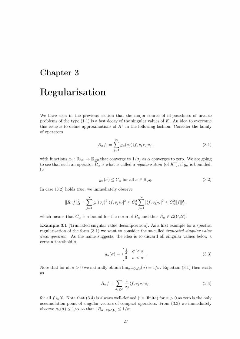
We have seen in the previous section that the major source of ill-posedness of inverseproblems of the type (1.1) is a fast decay of the singular values of K. An idea to overcomethis issue is to define approximations of K† in the following fashion. Consider the familyof operators
Rαf :=
∞∑j=1
gα(σj)〈f, vj〉V uj , (3.1)
with functions gα : R>0 → R≥0 that converge to 1/σj as α converges to zero. We are goingto see that such an operator Rα is what is called a regularisation (of K†), if gα is bounded,i.e.
gα(σ) ≤ Cα for all σ ∈ R>0. (3.2)
In case (3.2) holds true, we immediately observe
‖Rαf‖2U =∞∑j=1
gα(σj)2|〈f, vj〉V |2 ≤ C2
α
∞∑j=1
|〈f, vj〉V |2 ≤ C2α‖f‖2V ,
which means that Cα is a bound for the norm of Rα and thus Rα ∈ L(V,U).
Example 3.1 (Truncated singular value decomposition). As a first example for a spectralregularisation of the form (3.1) we want to consider the so-called truncated singular valuedecomposition. As the name suggests, the idea is to discard all singular values below acertain threshold α
gα(σ) =
1σ σ ≥ α0 σ < α
. (3.3)
Note that for all σ > 0 we naturally obtain limα→0 gα(σ) = 1/σ. Equation (3.1) then readsas
Rαf =∑σj≥α
1
σj〈f, vj〉V uj , (3.4)
for all f ∈ V. Note that (3.4) is always well-defined (i.e. finite) for α > 0 as zero is the onlyaccumulation point of singular vectors of compact operators. From (3.3) we immediatelyobserve gα(σ) ≤ 1/α so that ‖Rα‖L(U ,V) ≤ 1/α.
27

28
U V
δu† ff δ
K†f δ
Rαfδ
K
Figure 3.1: Visualization of reconstruction from noisy data. While the Moore–Penrose inverse re-constructs optimally from noiseless data, its noise amplification renders it useless when small errorsare present in the data. A regularisation operator gives a robust solution while still approximatingthe Moore–Penrose inverse.
Example 3.2 (Tikhonov regularisation). The main idea behind Tikhonov regularisation1
is to shift the singular values of K∗K by a constant factor, which will be associated withthe regularisation parameter α. This shift can be realised via the function
gα(σ) =σ
σ2 + α. (3.5)
Again, we immediately observe that for all σ > 0 we have limα→0 gα(σ) = 1/σ. Further,we can estimate gα(σ) ≤ 1/(2
√α) due to σ2 + α ≥ 2
√ασ. The corresponding Tikhonov
regularisation (3.1) reads as
Rαf =∞∑j=1
σjσ2j + α
〈f, vj〉V uj . (3.6)
After getting an intuition about regularisation of the form (3.1) via examples, we wantto define what a regularisation actually is, and what properties come along with it.
Definition 3.1. Let K ∈ L(U ,V) be a bounded operator. A family Rαα>0 of continuousoperators is called regularisation (or regularisation operator) of K† if
Rαf → K†f = u†
for all f ∈ D(K†) as α→ 0.
Definition 3.2. We further call Rαα>0 a linear regularisation, if Definition 3.1 is sat-isfied together with the additional assumption
Rα ∈ L(V,U) ,
for all α ∈ R>0.
Hence, a regularisation is a pointwise approximation of the Moore–Penrose inversewith continuous operators, see Figure 3.1 for an illustration. As in the interesting casesthe Moore–Penrose inverse may not be continuous we cannot expect that the norms of aregularisation stay bounded as α→ 0. This is confirmed by the following results.
1Named after the Russian mathematician Andrey Nikolayevich Tikhonov (30 October 1906 - 7 October1993)
CHAPTER 3. REGULARISATION 29
Theorem 3.1 (Banach–Steinhaus e.g. [4, p. 78], [17, p. 173]). Let U ,V be Hilbert spacesand Kjj∈N ⊂ L(U ,V) a family of point-wise bounded operators, i.e. for all u ∈ U thereexists a constant C(u) > 0 with supj∈N ‖Kju‖V ≤ C(u). Then
supj∈N‖Kj‖L(U ,V) <∞ .
Corollary 3.1 ([17, p. 174]). Let U ,V be Hilbert spaces and Kjj∈N ⊂ L(U ,V). Thenthe following two conditions are equivalent:
(a) There exists K ∈ L(U ,V) such that
Ku = limj→∞
Kju for all u ∈ U .
(b) There is a dense subset X ⊂ U such that limj→∞Kju exists for all u ∈ X and
supj∈N‖Kj‖L(U ,V) <∞ .
Theorem 3.2. Let U , V be Hilbert spaces, K ∈ L(U ,V) and Rαα>0 a linear regularisa-tion as defined in Definition 3.2. If K† is not continuous, Rαα>0 cannot be uniformlybounded. In particular this implies the existence of an element f ∈ V with ‖Rαf‖U → ∞for α→ 0.
Proof. We prove the theorem by contradiction and assume that Rαα>0 is uniformlybounded. Hence, there exists a constant C with ‖Rα‖L(V,U) ≤ C for all α > 0. Due toDefinition 3.1, we have Rα → K† on D(K†). Corollary 3.1 then already implies K† ∈L(V,U), which is a contradiction to the assumption that K† is not continuous.
It remains to show the existence of the element f ∈ V with ‖Rαf‖U → ∞ for α → 0.If such an element would not exist, we could conclude Rαα>0 ⊂ L(V,U). However,Theorem 3.1 then implies that Rαα>0 has to be uniformly bounded, which contradictsthe first part of the proof.
With the additional assumption that ‖KRα‖L(V,V) is bounded, we can even show thatRαf diverges for all f 6∈ D(K†).
Theorem 3.3. Let K ∈ L(U ,V) and Rαα>0 be a linear regularisation of K†, and defineuα := Rαf . If
supα>0‖KRα‖L(V,V) <∞ ,
then ‖uα‖U →∞ for f /∈ D(K†).
Proof. The convergence in case of f ∈ D(K†) simply follows from Definition 3.1. Wetherefore only need to consider the case f /∈ D(K†). We assume that there exists a sequenceαk → 0 such that ‖uαk‖U is uniformly bounded. Then there exists a weakly convergentsubsequence uαkl with some limit u ∈ U , cf. [9, Section 2.2, Theorem 2.1]. As continuouslinear operators are also weakly continuous, we further have Kuαkl Ku. However, asKRα are uniformly bounded operators, we also conclude Kuαkl = KRαklf PR(K)
f forall f ∈ V (and not just f ∈ D(K†)), because of Corollary 3.1. Hence, we further concludef ∈ R(K) and therefore f ∈ D(K†) in contradiction to the assumption f /∈ D(K†).

30 3.1. PARAMETER-CHOICE STRATEGIES
highlow regularisation
high
low
error
data errorapproximation errortotal error
Figure 3.2: The total error between a regularised solution and the minimal norm solution decom-poses into the data error and the approximation error. These two errors have opposing trends: Fora small regularisation parameter α the error in the data gets amplified through the ill-posednessof the problem and for large α the operator Rα is a poor approximation of the Moore–Penroseinverse.
Usually we cannot expect f ∈ D(K†) for most applications, due to measurement andmodelling errors. However, we assume that there exists f ∈ D(K†) such that we have∥∥∥f − f δ∥∥∥
V≤ δ
for measured data f δ ∈ V. For linear regularisations we can split the total error betweenthe regularised solution of the noisy problem Rαf
δ and the minimal norm solution of thenoise-free problem u† = K†f as
‖Rαf δ − u†‖U ≤ ‖Rαf δ −Rαf‖U + ‖Rαf − u†‖U≤ δ‖Rα‖L(V,U)︸ ︷︷ ︸
data error
+ ‖Rαf −K†f‖U︸ ︷︷ ︸approximation error
. (3.7)
The first term of (3.7) is the data error ; this term unfortunately does not stay boundedfor α → 0, which we can conclude from Theorem 3.2. The second term, known as theapproximation error, however vanishes for α→ 0, due to the pointwise convergence of Rαto K†. Hence it becomes evident from (3.7) that a good choice of α depends on δ, andneeds to be chosen such that the approximation error becomes as small as possible, whilstthe data error is being kept at bay. See Figure 3.2 for a visualisation of this situation. Inthe following we are going to discuss typical strategies for choosing α appropriately.
3.1 Parameter-choice strategies
In this section we want to discuss three standard rules for the choice of the regularisationparameter α and whether they lead to (convergent) regularisation methods.

CHAPTER 3. REGULARISATION 31
Definition 3.3. A function α : R>0 × V → R>0, (δ, f δ) 7→ α(δ, f δ) is called parameterchoice rule. We distinguish between
(a) a-priori parameter choice rules, if they depend on δ only;
(b) a-posteriori parameter choice rules, if they depend on δ and f δ;
(c) heuristic parameter choice rules, if they depend on f δ only.
In case of (a) or (c) we would simply write α(δ), respectively α(f δ), instead of α(δ, f δ).
Definition 3.4. If Rαα>0 is a regularisation of K† and α is a parameter choice rule,then the pair (Rα, α) is called convergent regularisation, if for all f ∈ D(K†) there existsa parameter choice rule α : R>0 × V → R>0 such that
limδ→0
sup∥∥∥Rαf δ −K†f∥∥∥
U
∣∣∣ f δ ∈ V,∥∥∥f − f δ∥∥∥V≤ δ
= 0 (3.8)
and
limδ→0
supα(δ, f δ)
∣∣∣ f δ ∈ V,∥∥∥f − f δ∥∥∥V≤ δ
= 0 (3.9)
are guaranteed.
3.1.1 A-priori parameter choice rules
First of all we want to discuss a-priori parameter choice rules in more detail. In fact, itcan be shown that for every regularisation an a-priori parameter choice rule, and thus, aconvergent regularisation, exists.
Theorem 3.4. Let Rαα>0 be a regularisation of K†, for K ∈ L(U ,V). Then there existsan a-priori parameter choice rule, such that (Rα, α) is a convergent regularisation.
Proof. Let f ∈ D(K†) be arbitrary but fixed. We can find a monotone increasing functionγ : R>0 → R>0 with limε→0 γ(ε) = 0 such that for every ε > 0 we have∥∥∥Rγ(ε)f −K†f
∥∥∥U≤ ε
2,
due to the pointwise convergence Rα → K†.As the operator Rγ(ε) is continuous for fixed ε, there exists ρ(ε) > 0 with∥∥Rγ(ε)g −Rγ(ε)f
∥∥U ≤
ε
2for all g ∈ V with ‖g − f‖V ≤ ρ(ε) .
Without loss of generality we can assume ρ to be a continuous, strictly monotone increasingfunction with limε→0 ρ(ε) = 0. Then, due to the inverse function theorem there exists astrictly monotone and continuous function ρ−1 on R(ρ) with limδ→0 ρ
−1(δ) = 0. Wecontinuously extend ρ−1 on R>0 and define our a-priori strategy as
α : R>0 → R>0, δ → γ(ρ−1(δ)) .
Then limδ→0 α(δ) = 0 follows. Furthermore, there exists δ := ρ(ε) for all ε > 0, such thatwith α(δ) = γ(ε)∥∥∥Rα(δ)f
δ −K†f∥∥∥U≤∥∥∥Rγ(ε)f
δ −Rγ(ε)f∥∥∥U
+∥∥∥Rγ(ε)f −K†f
∥∥∥U≤ ε
follows for all f δ ∈ V with ‖f − f δ‖V ≤ δ. Thus, (Rα, α) is a convergent regularisationmethod.

32 3.1. PARAMETER-CHOICE STRATEGIES
For linear regularisations we can characterise a-priori parameter choice strategies thatlead to convergent regularisation methods via the following theorem.
Theorem 3.5. Let Rαα>0 be a linear regularisation, and α : R>0 → R>0 an a-prioriparameter choice rule. Then (Rα, α) is a convergent regularisation method if and only if
(a) limδ→0 α(δ) = 0
(b) limδ→0 δ‖Rα(δ)‖L(V,U) = 0
Proof. ⇐: Let condition a) and b) be fulfilled. From (3.7) we then observe∥∥∥Rα(δ)fδ −K†f
∥∥∥U→ 0 for δ → 0.
Hence, (Rα, α) is a convergent regularisation method.⇒: Now let (Rα, α) be a convergent regularisation method. We prove that conditions 1and 2 have to follow from this by showing that violation of either one of them leads toa contradiction to (Rα, α) being a convergent regularisation method. If condition a) isviolated, (3.9) is violated and hence, (Rα, α) is not a convergent regularisation method. Ifcondition a) is fulfilled but condition b) is violated, there exists a null sequence δkk∈Nwith δk‖Rα(δk)‖L(V,U) ≥ C > 0, and hence, we can find a sequence gkk∈N ⊂ V with‖gk‖V = 1 and δk‖Rα(δk)gk‖U ≥ C for some C. Let f ∈ D(K†) be arbitrary and definefk := f + δkgk. Then we have on the one hand ‖f − fk‖V ≤ δk, but on the other hand thenorm of
Rα(δk)fk −K†f = Rα(δk)f −K†f + δkRα(δk)gk
cannot converge to zero, as the second term δkRα(δk)gk is bounded from below by con-struction. Hence, (3.8) is violated for f δ = gk and thus, (Rα, α) is not a convergentregularisation method.
3.1.2 A-posteriori parameter choice rules
In the following sections we are going to see that Theorem 3.5 basically means that α(δ)cannot converge too quickly to zero in relation to δ; typical parameter choice strategies willbe of the form α(δ) = δp. However, finding an optimal choice of p often requires additionalinformation about u†, for instance in terms of source conditions that we are going to discussin Section 3.2.4. A-posteriori parameter choice rules have the advantage that they do notrequire this additional information. The basic idea is as follows. We again have f ∈ D(K†)and f δ with ‖f − f δ‖V ≤ δ, and now consider the residual between f δ and uα := Rαf
δ,i.e.
‖Kuα − f δ‖V .
If we assume that u† is the minimal norm solution and f is given via f = Ku†, weimmediately observe that u† satisfies
‖Ku† − f δ‖V = ‖f − f δ‖V = δ .
Hence, it appears not to be useful to choose α(δ, f δ) with ‖Kuα(δ,fδ) − f δ‖V < δ, whichmotivates Morozov’s discrepany principle.

CHAPTER 3. REGULARISATION 33
Definition 3.5 (Morozov’s discrepancy principle). Let α(δ, f δ) be chosen such that
‖Kuα(δ,fδ) − f δ‖V ≤ ηδ (3.10)
is satisfied, for given δ, f δ, and a fixed constant η > 1. Then uα(δ,fδ) = Rα(δ,fδ)fδ is said
to satisfy Morozov’s discrepancy principle.
Remark 3.1. It is important to point out that (3.10) may never be fulfilled, as is the casefor f ∈ R(K)⊥. Following Lemma 2.3 (d), even for exact data f δ = f we observe
‖Ku† − f‖V = ‖KK†f − f‖V = ‖PR(K)f − f‖V = ‖f‖V > δ
in this case, for δ being small enough. In order to avoid this scenario, we ideally ensurethat R(K) is dense in V, as this already implies R(K)⊥ = 0 due to Remark 2.1.
Practical a-posteriori regularisation strategies are usually designed as follows. We picka null sequence αjj∈N and iteratively compute uαj = Rαjf
δ for j ∈ 1, . . . , j∗, j∗ ∈ N,until uαj∗ satisfies (3.10). This procedure is justified by the following theorem.
Theorem 3.6. Let Rαα>0 be a regularisation of K ∈ L(U ,V), and let R(K) be densein V. Further, let αjj∈N be a strictly monotonically decreasing null sequence, and letη > 1. If the family of operators KRαα>0 is uniformly bounded, there exists a finiteindex j∗ ∈ N such that for all f ∈ D(K†) and f δ with ‖f − f δ‖V ≤ δ the inequalities
‖Kuαj∗ − f δ‖V ≤ ηδ < ‖Kuαj − f δ‖V
are satisfied for all j < j∗.
Proof. We know that KRα converges pointwise to KK† = PR(K)in D(K†), which together
with the uniform boundedness assumption already implies pointwise convergence in V, aswe have already shown in the proof of Theorem 3.2. Hence, for all f ∈ D(K†) and f δ ∈ Vwith ‖f − f δ‖V ≤ δ we can conclude
limj→∞
‖Kuαj − f δ‖V = limj→∞
‖KRαjf δ − f δ‖V =∥∥∥PR(K)
f δ − f δ∥∥∥V
= infg∈R(K)
‖g − f δ‖V ≤ ‖f − f δ‖V ≤ δ .
We are going to demonstrate later that (3.10) in combination with specific regularisa-tions is indeed a regularisation method. Before we do so, we want to conclude the discussionof parameter choice strategies by investigating heuristic regularisation methods.
3.1.3 Heuristic parameter choice rules
Heuristic parameter choice rules do not require knowledge of the noise level δ, which makesthem popular strategies in practice. In the following we give three examples of popularheuristic parameter choice rules.
Quasi-optimality principle For the first n elements of a null sequence, i.e. αjj∈1,...,n,we choose α(f δ) = αj∗ with
j∗ = arg min1≤j<n
‖uαj+1 − uαj‖U .

34 3.2. SPECTRAL REGULARISATION METHODS
Hanke-Raus rule The parameter α(f δ) is chosen via
α(f δ) = arg minα>0
1√α‖Kuα − f δ‖V .
L-curve method The parameter α(f δ) is chosen via
α(f δ) = arg minα>0
‖uα‖U‖Kuα − f δ‖V .
Despite their popularity and the fact that they do not require any knowledge about δ,heuristic parameter choice rules have one significant theoretical disadvantage. While anyregularisation can be equipped with an a-priori parameter choice rule to form a convergentregularisation as seen in Theorem 3.4, heuristic parameter choice rules cannot lead toconvergent regularisations, a result that has become famous as the so-called Bakushinskiıveto [2].
Theorem 3.7. Let K ∈ L(U ,V) with R(K) 6= R(K). Then for any regularisationRαα>0 and any heuristic parameter choice rule α(f δ) the pair (Rα, α) is not a con-vergent regularisation.
Proof. Assume that (Rα, α) is a convergent regularisation method and that the param-eter choice rule is heurstic, i.e. α = α(f δ). Then it follows from (3.8) that
limδ→0
sup∥∥∥Rα(fδ)f
δ −K†f∥∥∥U
∣∣∣ f δ ∈ V,∥∥∥f − f δ∥∥∥V≤ δ
= 0
and in particular Rα(f)f = K†f for all f ∈ D(K†). Thus, for any sequence fjj∈N ⊂D(K†) which converges to f ∈ D(K†) we have that
limj→∞
K†fj = limj→∞
Rα(fj)fj = K†f
which shows that K† is continuous. It follows from Theorem 2.5 that the range of K isclosed, which contradicts the assumption.
Remark 3.2. We want to point out that Theorem 3.7 does not automatically make anyheuristic parameter choice rule useless, for two reasons. Firstly, because Theorem 3.7applies to infinite dimensional problems. Hence, discretised, ill-conditioned problems canstill benefit from heuristic parameter choice rules. Secondly, the proof of Theorem 3.7explicitly uses perturbed data fj ∈ D(K†) to show the contradiction. For actual perturbeddata f δ however, it is quite unusual that they will satisfy f δ ∈ D(K†). It can indeed beshown that, under the additional assumption f δ 6∈ D(K†), a lot of regularisation strategiestogether with a whole class of heuristic parameter choice strategies can be turned intoconvergent regularisations.
3.2 Spectral regularisation methods
Now we revisit (3.1) and finally prove that these methods are regularisation methods forpiecewise continuous functions gα satisfying (3.2).

CHAPTER 3. REGULARISATION 35
Theorem 3.8. Let gα : R>0 → R be a piecewise continuous function satisfying (3.2),limα→0 gα(σ) = 1
σ and
supα,σ
σgα(σ) ≤ γ , (3.11)
for some constant γ > 0. If Rα is defined as in (3.1), we have
Rαf → K†f as α→ 0,
for all f ∈ D(K†).
Proof. From the singular value decomposition of K† and the definition of Rα we obtain
Rαf −K†f =
∞∑j=1
(gα(σj)−
1
σj
)〈f, vj〉V uj =
∞∑j=1
(σjgα(σj)− 1) 〈u†, uj〉U uj .
From (3.11) we can conclude∣∣∣(σjgα(σj)− 1) 〈u†, uj〉U∣∣∣ ≤ (1 + γ)‖u†‖U ,
and hence, each element of the sum stays bounded. Thus, we can also estimate
‖Rαf −K†f‖2U =
∞∑j=1
|σjgα(σj)− 1|2∣∣∣〈u†, uj〉U ∣∣∣2 ≤ (1 + γ)2
∞∑j=1
∣∣∣〈u†, uj〉U ∣∣∣2= (1 + γ)2‖u†‖2U <∞
and conclude that ‖Rαf −K†f‖U is bounded from above. This allows the application ofthe reverse Fatou lemma, which yields the estimate
lim supα→0
∥∥∥Rαf −K†f∥∥∥2
U≤ lim sup
α→0
∞∑j=1
|σjgα(σj)− 1|2∣∣∣〈u†, uj〉U ∣∣∣2
≤∞∑j=1
∣∣∣ limα→0
σjgα(σj)− 1∣∣∣2 ∣∣∣〈u†, uj〉U ∣∣∣2 .
Due to the pointwise convergence of gα(σj) to 1/σj we obtain limα→0 σjgα(σj) − 1 = 0.Hence, we have
∥∥Rαf −K†f∥∥U → 0 for α→ 0 for all f ∈ D(K†).
Proposition 3.1. Let the same assumptions hold as in Theorem 3.8. Further, let α be ana-priori parameter choice rule. Then (Rα(δ), α(δ)) is a convergent regularisation method if
limδ→0
δCα(δ) = 0
is guaranteed.
Proof. The result follows immediately from ‖Rα(δ)‖L(V,U) ≤ Cα(δ) and Theorem 3.5.
36 3.2. SPECTRAL REGULARISATION METHODS
3.2.1 Convergence rates
Knowing that spectral regularisation methods of the form (3.1) together with (3.2) repre-sent convergent regularisation methods, we now want to understand how the error in thedata propagates to the error in the reconstruction.
Theorem 3.9. Let the same assumptions hold for gα as in Theorem 3.8. If we defineuα := Rαf and uδα := Rαf
δ, with f ∈ D(K†), f δ ∈ V and ‖f − f δ‖V ≤ δ, then
‖Kuα −Kuδα‖V ≤ γδ , (3.12)
and
‖uα − uδα‖U ≤ Cαδ (3.13)
hold true.
Proof. From the singular value decomposition we can estimate
‖Kuα −Kuδα‖2V ≤∞∑j=1
σ2j gα(σj)
2|〈f − f δ, vj〉V |2
≤ γ2∞∑j=1
|〈f − f δ, vj〉V |2 = γ2‖f − f δ‖2V ≤ γ2δ2 ,
which yields (3.12). In the same fashion we can estimate
‖uα − uδα‖2U ≤∞∑j=1
gα(σj)2|〈f − f δ, vj〉V |2
≤ C2α
∞∑j=1
|〈f − f δ, vj〉V |2 = C2α‖f − f δ‖2V ≤ C2
αδ2 ,
to obtain (3.13).
Remark 3.3. At first glance (3.13) gives the impression as if the error in the reconstructionis also of order δ. This, however, is not the case, as Cα also depends on δ, as we have seenin Proposition 3.1. The condition limδ→0 δCα = 0 will in particular force Cα to decay morequickly than δ. Hence, Cαδ will be of order δν , with 0 < ν < 1.
Combining the assertions of Theorem 3.8, Proposition 3.1 and Theorem 3.9, we obtainthe following convergence results of the regularised solutions.
Proposition 3.2. Let the assumptions of Theorem 3.8, Proposition 3.1 and Theorem 3.9hold true. Then,
uα(δ) → u†
is guaranteed as δ → 0.
CHAPTER 3. REGULARISATION 37
3.2.2 Truncated singular value decomposition
As a first example for a spectral regularisation of the form (3.1) we have considered theso-called truncated singular value decomposition in Example 3.1. From (3.3) we imme-diately observe gα(σ) ≤ Cα = 1/α. Thus, according to Proposition 3.1 the truncatedsingular value decomposition, together with an a-priori parameter choice strategy satisfy-ing limδ→0 α(δ) = 0, is a convergent regularisation method if limδ→0 δ/α(δ) = 0.
Moreover, we observe supσ,α σgα(σ) = γ = 1 and hence, we obtain the error estimates‖Kuα −Kuδα‖V ≤ δ and ‖uα − uδα‖U ≤ δ/α(δ) as a consequence of Theorem 3.9.
Let K ∈ K(U ,V) with singular system σj , uj , vj)j∈N, and choose for δ > 0 an indexfunction j∗ : R>0 → N with j∗(δ) → ∞ for δ → 0 and limδ→0 δ/σj∗(δ) = 0. We canthen choose α(δ) = σj∗(δ) as our a-priori parameter choice rule to obtain a convergentregularisation.
Note that in practice a larger δ implies that more and more singular values have to becut off in order to guarantee a stable recovery that successfully suppresses the data error.
3.2.3 Tikhonov regularisation
The second example we were considering was Tikhonov regularisation in Example 3.2,where we have shifted the singular values of K∗K by a constant factor, which will beassociated with the regularisation parameter α.
In case of gα as defined in (3.5) we observe limα→0 gα(σ) = 1/σ for σ > 0. Further,we can estimate gα(σ) ≤ 1/(2
√α) = Cα due to σ2 + α ≥ 2
√ασ. Moreover, we discover
σgα(σ) = σ2/(σ2 +α) < 1 =: γ for α > 0. Consequently, we have to ensure δ/(2√α(δ))→
0 for δ → 0 to obtain a convergent regularisation, and in that case get the estimates‖Kuα −Kuδα‖V ≤ δ and ‖uα − uδα‖U ≤ δ/(2
√α(δ)). Thus, equipping Rα(δ) for instance
with the a-priori parameter choice rule α(δ) = δ/4 will lead to a convergent regularisationfor which we have ‖uα − uδα‖U = O(
√δ).
Note that Tikhonov regularisation can be computed without knowledge of the singularsystem. Considering the equation (K∗K + αI)uα in terms of the singular value decompo-sition, we observe
∞∑j=1
σjσ2j + α
〈f, vj〉V K∗ Kuj︸︷︷︸=σjvj︸ ︷︷ ︸
=σ2juj
+∞∑j=1
ασjσ2j + α
〈f, vj〉V uj
=∞∑j=1
σj(σ2j + α)
σ2j + α
〈f, vj〉V uj =∞∑j=1
σj〈f, vj〉V uj = K∗f .
Hence, the Tikhonov-regularised solution uα can be obtained by solving
(K∗K + αI)uα = K∗f (3.14)
for uα. The advantage in computing uα via (3.14) is that its computation does not requirethe singular value decomposition ofK, but only involves the inversion of a linear, well-posedoperator equation with a symmetric, positive definite operator.
3.2.4 Source-conditions
Before we continue to investigate other examples of regularisations we want to brieflyaddress the question of the convergence speed of a regularisation method. From Theorem

38 3.2. SPECTRAL REGULARISATION METHODS
3.9 we have already obtained a convergence rate result; however, with additional regularityassumptions on the (unknown) minimal norm solution we are able to improve those. Theregularity assumptions that we want to consider are known as source conditions, and areof the form
∃w ∈ U : u† = (K∗K)µw . (3.15)
The power µ > 0 of the operator is understood in the sense of the consider the µ-th powerof the singular values of the operator K∗K, i.e.
(K∗K)µw =∞∑j=1
σ2µj 〈w, uj〉Uuj .
Example 3.3 (Differentiation). We want to take a look at what (3.15) actually meansin the case of a specific example. We therefore again consider the inverse problem ofdifferentiation, i.e.
(Ku)(y) =
∫ y
0u(x) dx .
In case of µ = 1 (3.15) reads as
u†(x) =
∫ 1
x
∫ y
0w(z) dz dy .
due to (2.10). Hence, (3.15) does simply imply that u† has to be twice weakly differentiable.It becomes even more obvious if we look at twice differentiable u†. In that case applyingthe Leibniz differentiation rule for parameter integrals leaves us with
(u†)′′(x) = −w(x) .
Hence, any twice differentiable u† automatically satisfies the source condition (3.15) forµ = 1.Similar results follow for different choices of µ ∈ N.
The rate of convergence of a regularisation scheme to the minimal norm solution nowdepends on the specific choice of gα. We assume that gα satisfies
σ2µ|σgα(σ)− 1| ≤ ωµ(α) ,
for all σ > 0. In case of the truncated singular value decomposition we would for instancehave ωµ(α) = α2µ. With this additional assumption, we can improve the estimate inTheorem 3.8 as follows:
‖Rαf −K†f‖2V ≤∞∑j=1
|σjgα(σj)− 1|2|〈u†, uj〉U |2
=
∞∑j=1
|σjgα(σj)− 1|2σ4µj |〈w, uj〉U |2
≤ ωµ(α)2‖w‖2UHence, we have obtained the estimate
‖uα − u†‖U ≤ ωµ(α)‖w‖U .Together with (3.7) we can further estimate
‖uα(δ) − u†‖U ≤ ωµ(α)‖w‖U + Cαδ . (3.16)

CHAPTER 3. REGULARISATION 39
Example 3.4. In case of the truncated singular value decomposition we know from Section3.2.2 that Cα = 1/α, and we can further conclude ωµ(α) = α2µ. Hence, (3.16) simplifiesto
‖uα(δ) − u†‖U ≤ α2µ‖w‖U + δα−1 (3.17)
in this case. In order to make the right-hand-side of (3.17) as small as possible, we haveto choose α such that
α =
(δ
2µ‖w‖U
) 12µ+1
.
With this choice of α we estimate
‖uα(δ) − u†‖U ≤ 21−2µ1+2µ︸ ︷︷ ︸≤2
µ1−2µ1+2µ︸ ︷︷ ︸≤1
δ2µ
2µ+1 ‖w‖1
2µ+1
U
≤ 2δ2µ
2µ+1 ‖w‖1
2µ+1
U .
It is important to note that no matter how large µ is, the rate of convergence δ2µ
2µ+1 willalways be slower than δ, due to the ill-posedness of the inversion of K.
3.2.5 Asymptotic regularisation
Another form of regularisation is asymptotic regularisation of the form
∂tu(t) = K∗ (f −Ku(t))
u(0) = 0. (3.18)
As the linear operator K does not change with respect to the time t, we can make theAnsatz of writing u(t) in terms of the singular value decomposition of K as
u(t) =
∞∑j=1
γj(t)uj , (3.19)
for some function γ : R→ R. From the initial conditions we immediately observe γ(0) = 0.From the singular value decomposition and (3.18) we further see
∞∑j=1
γ′j(t)uj =∞∑j=1
σj
〈f, vj〉V − σjγ(t) 〈uj , uj〉U︸ ︷︷ ︸=‖uj‖2U=1
uj .
Hence, by equating the coefficients we get
γ′j(t) = σj〈f, vj〉V − σ2j γj(t) ,
and together with γj(0) we obtain
γj(t) =(
1− e−σ2j t) 1
σj〈f, vj〉V

40 3.2. SPECTRAL REGULARISATION METHODS
as a solution for all j and hence, (3.19) reads as
u(t) =∞∑j=1
(1− e−σ2
j t) 1
σj〈f, vj〉Vuj .
If we substitute t = 1/α, we obtain the regularisation
uα =
∞∑j=1
(1− e−
σ2jα
)1
σj〈f, vj〉Vuj
with gα(σ) =
(1− e−σ
2
α
)1σ . We immediately see that gα(σ)σ ≤ 1 =: γ, and due to
ex ≥ 1 +x we further observe 1− e−σ2
α ≤ σ2/α and therefore (1− e−σ2
α )/σ ≤ maxj σj/α =σ1/α = ‖K‖L(U ,V)/α =: Cα.
3.2.6 Landweber iteration
If we approximate (3.18) via a forward finite-difference discretisation, we end up with theiterative procedure
uk+1 − ukτ
= K∗(f −Kuk
), (3.20)
⇔ uk+1 = uk + τK∗(f −Kuk
),
⇔ uk+1 = (I − τK∗K)uk + τK∗f ,
for some τ > 0 and u0 ≡ 0. Iteration (3.20) is known as the so-called Landweber iteration.We assume f ∈ D(K†) first, and with the singular value decomposition of K and K∗ weobtain
∞∑j=1
〈uk+1, uj〉Uuj =
∞∑j=1
((1− τσ2
j
)〈uk, uj〉U + τσj〈f, vj〉V
)uj , (3.21)
and hence, by equating the individual summands
〈uk+1, uj〉U =(1− τσ2
j
)〈uk, uj〉U + τσj〈f, vj〉V . (3.22)
Assuming u0 ≡ 0, summing up equation (3.22) yields
〈uk, uj〉U = τσj〈f, vj〉Vk∑i=1
(1− τσ2j )k−i . (3.23)
The following Lemma will help us simplifying (3.23).
Lemma 3.1. For k ∈ N \ 1 we have
k∑i=1
(1− τσ2)k−i =1−
(1− τσ2
)kτσ2
. (3.24)
CHAPTER 3. REGULARISATION 41
Proof. Equation (3.24) can simply be verified via induction. We immediately see that
2∑i=1
(1− τσ2)2−i = 1 + (1− τσ2) =1− (1− 2τσ2 + τ2σ4)
τσ2=
1−(1− τσ2
)2τσ2
serves as as our induction base. Considering k → k + 1, we observe
k+1∑i=1
(1− τσ2)k+1−i = 1 +k∑i=1
(1− τσ2)k+1−i
= 1 + (1− τσ2)
k∑i=1
(1− τσ2)k−i
= 1 + (1− τσ2)1−
(1− τσ2
)kτσ2
=1−
(1− τσ2
)k+1
τσ2,
and we are done.
If we now insert (3.24) into (3.23) we therefore obtain
〈uk, uj〉U =(
1− (1− τσ2j )k) 1
σj〈f, vj〉V . (3.25)
The important consequence of Equation (3.25) is that we now immediately see that 〈uk, uj〉U →〈u†, uj〉U if we ensure (1 − τσ2
j )k → 0. In other words, we need to choose τ such that
|1− τσ2j | < 1 (respectively 0 < τσj < 2) for all j. As in the case of asymptotic regularisa-
tion we exploit that σ1 = ‖K‖L(U ,V) > σj for all j and select τ such that
0 < τ <2
‖K‖2L(U ,V)
(3.26)
is satisfied. If we interpret the iteration number as the regularisation parameter α := 1/k,we obtain the regularisation method
uα = Rαf =∞∑j=1
(1−
(1− τσ2
j
) 1α
) 1
σj〈f, vj〉V
with gα(σ) =(
1− (1− τσ2)1α
)/σ.
Landweber Iteration & the discrepancy principle
To conclude this section on the Landweber iteration we want to prove convergence ratesgiven u† satisfies a source condition. We further want to demonstrate that Landweberiteration in combination with the a-posteriori parameter choice rule defined in Definition3.5 is a sensible strategy that ensures uk → u† as long as the discrepancy principle isviolated. Following the introduction of the source condition in Section 3.2.4, we want toassume a source condition similar (3.15) for µ = 1/2, i.e. there exists a w ∈ V such that
u† = K∗w (3.27)
is satisfied. Under that additional assumption we can conclude the following convergencerate in the case of noise-free data f δ = f .
42 3.2. SPECTRAL REGULARISATION METHODS
Lemma 3.2. Let (3.27) be satisfied. Then the Landweber iterates (3.20) satisfy
‖uk − u†‖U = O(
1√k
)= O
(√α),
for f = Ku†.
Proof. We start proving this statement by showing that the inner product of uk − u† witha singular vector uj simplifies to
〈uk − u†, uj〉U = 〈uk, uj〉U − 〈u†, uj〉U=(
1− (1− τσ2j )k)〈u†, uj〉U − 〈u†, uj〉U
= (1− τσ2j )k〈u†, uj〉U
= σj(1− τσ2j )k︸ ︷︷ ︸
=:r(σj)
〈w, uj〉U ,
with the second equality following from Equation (3.25). As our next step, we want to findan upper bound for r(σj). We therefore analyse the concave function r(σ) = σ(1− τσ2)k
by computing its first derivative, setting it to zero and inserting the resulting argumentthat maximises r. This yields
maxσ
r(σ) =
(2k
2k+1
)k√τ(2k + 1)
≤ 1√τ(2k + 1)
for k ∈ N. Hence, we obtain the estimate
∣∣∣〈uk − u†, uj〉U ∣∣∣ ≤ |〈w, uj〉U |√τ(2k + 1)
,
and consequently
‖uk − u†‖U =
√√√√ ∞∑j=1
|〈uk − u†, uj〉U |2 ≤1√
τ(2k + 1)
√√√√ ∞∑j=1
|〈w, uj〉U |2 =‖w‖U√τ(2k + 1)
.
Together with the stepsize-constraint (3.26) we can further conclude convergence of theiterates to a least squares solution.
Lemma 3.3. Let (3.26) be satisfied. Then the iterates (3.20) satisfy
‖Kuk+1 − f‖V ≤ ‖Kuk − f‖V ,
for f = Ku† and all k ∈ N, where equality only holds if uk already satisfies the normalequation (2.3).

CHAPTER 3. REGULARISATION 43
Proof. We easily estimate
‖Kuk+1 − f‖2V = ‖K(I − τK∗K)uk − (I − τK∗)f‖2V= ‖Kuk − f − τKK∗(Kuk − f)‖2V= ‖Kuk − f‖2V − 2τ〈K∗(Kuk − f),K∗(Kuk − f)〉U + τ2‖KK∗(Kuk − f)‖2V= ‖Kuk − f‖2V + τ
(τ‖KK∗(Kuk − f)‖2V − 2‖K∗(Kuk − f)‖2U
)≤ ‖Kuk − f‖2V + τ‖K∗(Kuk − f)‖2U
(τ‖K‖2L(U ,V) − 2
)︸ ︷︷ ︸
<0
≤ ‖Kuk − f‖2V ,
which proves the statement.
Lemma 3.2 and Lemma 3.3 allow us to conclude the following proposition.
Proposition 3.3. The Landweber iteration is a linear regularisation in the sense of Defi-nition 3.2.
In order to show that the Landweber iteration (3.20) in combination with the discrep-ancy principle (3.10) is also a convergent regularisation, we obviously have to look at thecase of noisy data f δ with ‖f δ − f‖V ≤ δ for f = Ku†. We denote the solution of (3.20)in case of noisy data f δ as ukδ for all k ∈ N and obtain the following estimate for the normbetween ukδ and u†.
Lemma 3.4. Let (3.27) be satisfied. Then the Landweber iterates (3.20) satisfy
‖ukδ − u†‖U ≤ τkδ‖K‖L(U ,V) +‖w‖U√τ(2k − 1)
(3.28)
for k ∈ N \ 1, f = Ku†, f δ ∈ V and ‖f δ − f‖V ≤ δ.
Proof. Similar to the proof of Lemma 3.2 we consider the inner product between ukδ − u†and a singular vector uj , which yields
〈ukδ − u†, uj〉U =1
σj
((1− (1− τσ2
j )k)〈f δ, vj〉V − 〈f, vj〉V
)=
1
σj
(1− (1− τσ2
j )k)〈f δ − f, vj〉V − σj(1− τσ2
j )k〈w, vj〉V .
Hence, for k > 1 we can use (3.24) to estimate
1
σj
(1− (1− τσ2
j )k) ∣∣∣〈f δ − f, vj〉V ∣∣∣ = τσj
k∑j=1
(1− τσ2j )k−j
∣∣∣〈f δ − f, vj〉V ∣∣∣≤ τkσj
∣∣∣〈f δ − f, vj〉V ∣∣∣ ≤ τkσ1
∣∣∣〈f δ − f, vj〉V ∣∣∣ .Together with the result from Lemma 3.2 we conclude
‖ukδ − u†‖U ≤ τkδ‖K‖L(U ,V) +‖w‖U√τ(2k − 1)
.
44 3.3. TIKHONOV REGULARISATION REVISITED
Note that the decrease of the residual in Lemma 3.3 holds true for all f ∈ V. As weobviously do not want to iterate until infinity – this would blow up the data error in (3.28)– this decrease together with the stepsize-constraint (3.26) motivates the use of (3.10) asa stopping criterion. The following lemma shows that with (3.20) we indeed minimise thedifference between ukδ and u† (in terms of the U norm) as long as (3.10) is violated.
Lemma 3.5. Let (3.26) be satisfied. Then the iterates of (3.20) satisfy
‖uk+1δ − u†‖U ≤ ‖ukδ − u†‖U
for k ≤ k∗, f = Ku† and f δ ∈ V with ‖f δ − f‖V ≤ δ. Here, k∗ satisfies the discrepancyprinciple (3.10) for η = 2/(2 − τ‖K‖2L(U ,V)) > 1. Moreover, equality can only be attainedfor δ = 0 and ukδ satisfying the normal equation (2.3).
Proof. We prove the statement by showing that ‖uk+1δ − u†‖2U − ‖ukδ − u†‖2U is negative
whilst the discrepancy principle is not violated. We estimate
‖uk+1δ − u†‖2U − ‖ukδ − u†‖2U = ‖ukδ − τK∗(Kukδ − f δ)− u†‖2U − ‖ukδ − u†‖2U
= τ2‖K∗(Kukδ − f δ)‖2U − 2τ〈Kukδ − f δ,Kukδ − f〉V≤ τ2‖K‖2L(U ,V)‖Kukδ − f δ‖2V − 2τ 〈Kukδ − f δ,Kukδ − f + f δ − f δ〉V︸ ︷︷ ︸
=‖Kukδ−fδ‖2V+〈Kukδ−fδ,fδ−f〉V
= τ(τ‖K‖2L(U ,V) − 2
)‖Kukδ − f δ‖2V + 2τ〈f − f δ,Kukδ − f δ〉V
≤ τ(τ‖K‖2L(U ,V) − 2
)‖Kukδ − f δ‖2V + 2τδ‖Kukδ − f δ‖V
= −τ‖Kukδ − f δ‖V((
2− τ‖K‖2L(U ,V)
)‖Kukδ − f δ‖V − 2δ
)= −2τ
η‖Kukδ − f δ‖V
(‖Kukδ − f δ‖V − ηδ
).
Hence, for k ≤ k∗ we conclude ‖uk+1δ − u†‖U ≤ ‖ukδ − u†‖U .
3.3 Tikhonov regularisation revisited
We conclude this chapter by showing that Tikhonov regularisation can not just be in-terpreted as the spectral regularisation (3.6) and the solution of the well-posed operatorequation (3.14), but also as the minimiser of a functional.
Theorem 3.10. For f ∈ V the Tikhonov-regularised solution uα = Rαf with Rα as definedin (3.6) is uniquely determined as the global minimiser of the Tikhonov-functional
Tα(u) :=1
2‖Ku− f‖2V +
α
2‖u‖2U . (3.29)
Proof. ⇒: Let uα be the Tikhonov-regularised solution and we show that it is also a globalminimiser. A global minimiser u ∈ U of Tα(u) is characterised via Tα(u) ≤ Tα(u) for all

CHAPTER 3. REGULARISATION 45
u ∈ U . Hence, it follows from
Tα(u)− Tα(uα) =1
2‖Ku− f‖2V +
α
2‖u‖2U −
1
2‖Kuα − f‖2V −
α
2‖uα‖2U
=1
2‖Ku‖2V − 〈Ku, f〉+
α
2‖u‖2U −
1
2‖Kuα‖2V + 〈Kuα, f〉 −
α
2‖uα‖2U
+ 〈(K∗K + αI)uα −K∗f, uα − u〉︸ ︷︷ ︸=0
=1
2‖Ku−Kuα‖2V +
α
2‖u− uα‖2U
≥ 0
that uα is a global minimiser of Tα.⇐: Let now u be a global minimiser. If we have Tα(u) ≤ Tα(u) (for all u ∈ U), it followswith u = u+ τv for arbitrary τ > 0 and fixed v ∈ U that
0 ≤ Tα(u)− Tα(u) =τ2
2‖Kv‖2V +
τ2α
2‖v‖2U + τ〈(K∗K + αI)u−K∗f, v〉U
holds true. Dividing by τ and subsequent consideration of the limit τ ↓ 0 thus yields
〈(K∗K + αI)u−K∗f, v〉U ≥ 0 , for all v ∈ U .
Thus (K∗K + αI)u − K∗f = 0 and we conclude u = uα, i.e. a global minimiser is theTikhonov-regularised solution. This also shows that the global minimiser of the Tikhonovfunctional (3.29) is unique.
This result paves the way for a generalisation of Tikhonov regularisation to a muchbroader class of regularisation methods that we want to discuss in the following chapter.

46 3.3. TIKHONOV REGULARISATION REVISITED

Chapter 4
Variational regularisation
At the end of the last chapter we have seen that Tikhonov regularisation1 Rαf can becharacterised as the solution of the minimisation problem
Rαf = arg minu∈U
1
2‖Ku− f‖2V +
α
2‖u‖2U
.
It is well known that the solution to an unconstrained minimisation problem has a vanishingderivative. In function spaces, the (Gâteaux-) derivative is also called the “first variation”such that minimisation problems are also called variational problems and methods thatrely on minimising a functional variational methods. In this section we want to investigatevariational methods for regularisation of linear inverse problems. To do so we will generaliseTikhonov regularisation by choosing different regularisation functionals J : U → R andcompute regularised solutions by minimising the functional
Φα,f (u) :=1
2‖Ku− f‖2V + αJ(u) .
Regularisation of this form is sometimes called Tikhonov-type regularisation but we willrefer to this as variational regularisation. Before we have a look at the theory behindvariational regularisation such as the existence and uniqueness of minimisers we will discussseveral examples of regularisation functionals J .
Example 4.1 (Tikhonov-Philipps regularisation). The easiest way to extend classicalTikhonov regularisation to a more general regularisation method is to replace 1
2‖u‖2U by12‖Du‖2Z where D : U → Z is a linear (not necessarily bounded) operator and we thusminimise
1
2‖Ku− f‖2V +
α
2‖Du‖2Z ,
which became known as Tikhonov-Philipps regularisation. While Tikhonov regularisationpenalises the norm of u, in Tikhonov-Philipps regularisation only certain features of u(depending on the choice of D) are penalised. The most frequent used operator D inimaging applications is the gradient operator ∇ such that the regulariser J correspondsto the semi-norm on H1(Ω) which is the Sobolev space of functions u ∈ L2(Ω) such thatthe weak derivative ∇u exists and ∇u ∈ L2(Ω,Rn). By using this regulariser, only thevariations in u but not the actual intensities are penalised which helps to control noisewithout a bias of the intensities towards zero.
1This regularisation is called ridge regression in the statistical literature.
47

48
If the operator D is given by Du = (u,∇u) and Z = L2(Ω) × L2(Ω,Rn) is equippedwith the natural inner product for product spaces, then
J(u) =1
2‖Du‖2Z =
1
2‖u‖2L2 +
1
2‖∇u‖2L2
is the norm on H1(Ω) and it corresponds to classical Tikhonov regularisation on H1(Ω).
Example 4.2 (`1-regularisation). When it comes to non-injective operators K ∈ L(`1, `2)between sequence spaces, the `1-norm, i.e. ‖u‖`1 :=
∑∞j=1 |uj | is often used as a regulariser,
in order to enforce sparse solutions. The corresponding minimisation problem reads as
minu∈`1
1
2‖Ku− f‖2`2 + α‖u‖1
. (4.1)
This problems is also called lasso in the statistical literature. One can show that minimisersof (4.1) are always sparse in the sense that they have finite support, i.e. | supp(u)| < ∞with supp(u) = i ∈ N |ui 6= 0. This is in contrast to solutions of the Tikhonov regularisedproblem which may not be sparse. For a finite dimensional example see Figure 4.1.
minimal `2-norm minimal `1-norm
Figure 4.1: Non-injective operators have a non-trivial kernel such that the inverse problem hasmore than one solution and the solutions form an affine subspace visualised by the solid line.Different regularisation functionals favour different solutions. The circle and the diamond indicateall points with constant `2-norm, respectively `1-norm, and the minimal `2-norm and `1-normsolutions are the intersections of the line with the circle, respectively the diamond. As it canbe seen, the minimal `2-norm solution has two non-zero components while the minimal `1-normsolution has only one non-zero component and thus is sparser.
Example 4.3 (Elastic net). Another regularisation method from statistics is the elasticnet, where the regulariser is the weighted sum of the `1-norm and the squared `2-norm:
J(u) = ‖u‖`1 +β
2‖u‖2`2 .
Here the idea is to combine two favorable models in order to get sparse solutions with morestability. As `1 ⊂ `2 we could either consider the elastic net on the Banach space `1 or onthe Hilbert space `2. In case we decide to do the latter, we can extend the elastic net suchthat
J(u) =
‖u‖`1 + β
2 ‖u‖2`2 if u ∈ `1∞ if u ∈ `2 \ `1
.

CHAPTER 4. VARIATIONAL REGULARISATION 49
Figure 4.2: The absolute value function on the left is in H1,1(Ω), Ω = [−1, 1], while the Heavisidefunction on the right is not. The solid dot at a jump indicates the value that the function takes.However, the Heaviside function is in BV(Ω) which shows that BV(Ω) is larger than H1,1(Ω).Moreover, it shows that BV(Ω) includes function with discontinuities which is a favourable modelfor images with sharp edges.
Intuitively, the value ∞ makes sure that a minimiser will never be in `2 \ `1 but we willdiscuss this aspect in more detail later.
Example 4.4 (Total variation). Total variation as a regulariser has originally been intro-duced for image-denoising and -restoration applications with the goal to preserve edges inimages, respectively discontinuities in signals [13]. For smooth signals u ∈ H1,1(Ω), i.e.u ∈ L1(Ω) and has a weak derivative ∇u ∈ L1(Ω,Rn), the total variation is simply definedas the semi-norm on the Sobolev space H1,1(Ω)
J(u) = TV(u) :=
∫Ω‖∇u(x)‖2 dx .
However, functions in H1,1(Ω) may not allow discontinuities which are useful in imagingapplications to model images with sharp edges.
To allow discontinuities while still preserving some regularity (otherwise we could modelimages in L1(Ω) for instance) we generalise the definition of the total variation. It is well-known (e.g. Cauchy–Schwarz inequality) that for x, v ∈ Rn with ‖v‖2 ≤ 1 we have that〈v, x〉 ≤ ‖x‖2. Thus, for any test function ϕ ∈ D(Ω,Rn) with
D(Ω,Rn) :=ϕ ∈ C∞0 (Ω;Rn)
∣∣∣ supx∈Ω‖ϕ(x)‖2 ≤ 1
we have that
TV(u) =
∫Ω‖∇u(x)‖2 dx ≥
∫Ω〈∇u(x), ϕ(x)〉 dx = −
∫Ωu(x) divϕ(x) dx
where the last equality is due to partial integration (Gauss’ divergence theorem). In factone can show that
TV(u) = supϕ∈D(Ω,Rn)
∫Ωu(x) divϕ(x) dx ,
which gives rise to the definition of functions of bounded variation.
BV(Ω) :=u ∈ L1(Ω)
∣∣∣ ‖u‖BV := ‖u‖L1 + TV(u) <∞
It can be shown that BV(Ω) is much larger than H1,1(Ω) and contains functions withdiscontinuities, see examples in Figure 4.2.

50 4.1. VARIATIONAL METHODS
Example 4.5 (Maximum-entropy regularisation). Maximum-entropy regularisation is ofparticular interest if solutions of the inverse problem are assumed to be probability densityfunctions (pdf), i.e. functions in the set
PDF(Ω) :=
u ∈ L1(Ω)
∣∣∣∣ ∫Ωu(x) dx = 1, u ≥ 0
.
The set PDF(Ω) is a convex subset but it is not a subspace as differences of pdfs arenot necessarily pdfs. The (differential) entropy used in physics and information theory isdefined as the functional PDF(Ω)→ R with
u 7→ −∫
Ωu(x) log(u(x)) dx
and the convention 0 log(0) := 0. As PDF(Ω) is not a vector space, we extend it to thewhole L1(Ω) and define the negative entropy regularisation as
J(u) =
∫Ω u(x) log(u(x)) dx if u ∈ PDF(Ω)
∞ else.
To summarise the introduction, variational regularisation aims at finding approxima-tions to the solution of the inverse problem (1.1) by minimising appropriate functionals ofthe form
Φα,f (u) :=1
2‖Ku− f‖2V + αJ(u) , (4.2)
where J : U → R ∪ ∞ represents a functional over the Banach space U , V is a Hilbertspace and K ∈ L(U ,V) a linear and continuous operator, and α > 0 is a real, positiveconstant. The term D(u) := 1
2‖Ku − f‖2V is usually named fidelity or data term, as itmeasures the deviation between the measured data f and the forward model Ku. Thefunctional J is the regularisation term or regulariser as it will impose certain regularityconditions on the unknown u. The regularisation parameter will balance between bothterms. Next, we will study some general theory on variational methods that will tellus under which conditions we can expect existence and uniqueness of solutions to thoseminimisation problems.
4.1 Variational methods
4.1.1 Background
Banach spaces and weak convergence
To cover all the examples of the beginning of this chapter we have to extend our settingto include Banach spaces. These are complete, normed vector spaces (as Hilbert spaces)but they may not have an inner product. For every Banach space U , we can define thespace of linear and continuous functionals which is called the dual space U∗ of U , i.e.U∗ := L(U ,R). Let u ∈ U and p ∈ U∗, then we usually write the dual product 〈p, u〉instead of p(u). Obviously, the dual product is not symmetric (in contrast to the innerproduct of Hilbert spaces). Moreover, for any K ∈ L(U ,V) there exists a unique operatorK∗ : V∗ → U∗, called the adjoint of K such that for all u ∈ U and p ∈ V∗ we have
〈K∗p, u〉 = 〈p,Ku〉 .
CHAPTER 4. VARIATIONAL REGULARISATION 51
It is easy to see that either side of the equation are well-defined, e.g. K∗p ∈ U∗ and u ∈ U .As the dual space is a Banach space, it has a dual space as well which we will call the
bi-dual space of U and denote it with U∗∗ := (U∗)∗. As every u ∈ U defines a continuousand linear mapping on the dual space U∗ by
〈E(u), p〉 := 〈p, u〉 ,
the mapping E : U → U∗∗ is well-defined. It can be shown that E is a linear and continuousisometry (and thus injective). In the special case when E is surjective, we call U reflexiv.Examples of reflexive Banach spaces include Hilbert spaces and Lq, `q spaces with 1 <q < ∞. We call the space U separable if there exists a set X ⊂ U of at most countablecardinality such that X = U .
A problem in infinite dimensional spaces is that bounded sequences may fail to haveconvergent subsequences. An example is for instance in `2 the sequence ukk∈N ⊂ `2, ukj =
1 if k = j and 0 otherwise. It is easy to see that ‖uk‖`2 = 1 and that there is no u ∈ `2such that uk → u. To circumvent this problem, we define a weaker topology on U . We saythat ukk∈N ⊂ U converges weakly to u ∈ U if and only if for all p ∈ U∗ the sequence ofreal numbers 〈p, uk〉k∈N converges and
〈p, uj〉 → 〈p, u〉 .
We will denote weak convergence by uk u. On a dual space U∗ we could define anothertopology (in addition to the strong topology induced by the norm and the weak topologyas the dual space is a Banach space as well). We say a sequence pkk∈N ⊂ U∗ convergesin weak-∗ to p ∈ U∗ if and only if
〈pk, u〉 → 〈p, u〉 for all u ∈ U
and we denote weak-∗ convergence by pk∗→ p. Similarly, for any topology τ on U we
denote the convergence in that topology by uk τ→ u.With these two new notions of convergence, we can solve the problem of bounded
sequences:
Theorem 4.1 (Sequential Banach-Alaoglu Theorem, e.g. [14, p. 70] or [15, p. 141]). LetU be a separable normed vector space. Then every bounded sequence ukk∈N ⊂ U∗ has aweak-∗ convergent subsequence.
Theorem 4.2 ([17, p. 64]). Each bounded sequence ukk∈N in a reflexive Banach spaceU has a weakly convergent subsequence.
Infinity calculus
We will look at functionals E : U → R∞ whose range is modelled to be the extended realline R∞ := R∪+∞ where the symbol ∞ denotes an element that is not part of the realline that is by definition larger than any other element of the reals, i.e.
x <∞
for all x ∈ R. This is useful to model constraints: For instance, if we were trying to minimiseE : [−1,∞)→ R, x 7→ x2 we could remodel this minimisation problem by E : R→ R∞
E(x) =
x2 if x ≥ −1
∞ else.
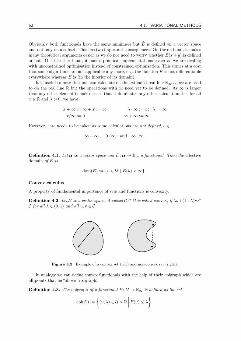
52 4.1. VARIATIONAL METHODS
Obviously both functionals have the same minimiser but E is defined on a vector spaceand not only on a subset. This has two important consequences: On the on hand, it makesmany theoretical arguments easier as we do not need to worry whether E(x+ y) is definedor not. On the other hand, it makes practical implementations easier as we are dealingwith unconstrained optimisation instead of constrained optimisation. This comes at a costthat some algorithms are not applicable any more, e.g. the function E is not differentiableeverywhere whereas E is (in the interior of its domain).
It is useful to note that one can calculate on the extended real line R∞ as we are usedto on the real line R but the operations with ∞ need yet to be defined. As ∞ is largerthan any other element it makes sense that it dominates any other calculation, i.e. for allx ∈ R and λ > 0, we have
x+∞ :=∞+ x :=∞ λ · ∞ :=∞ · λ :=∞x/∞ := 0 ∞+∞ :=∞ .
However, care needs to be taken as some calculations are not defined, e.g.
∞−∞ , 0 · ∞ and ∞ ·∞ .
.
Definition 4.1. Let U be a vector space and E : U → R∞ a functional. Then the effectivedomain of E is
dom(E) := u ∈ U | E(u) <∞ .
Convex calculus
A property of fundamental importance of sets and functions is convexity.
Definition 4.2. Let U be a vector space. A subset C ⊂ U is called convex, if λu+(1−λ)v ∈C for all λ ∈ (0, 1) and all u, v ∈ C.
Figure 4.3: Example of a convex set (left) and non-convex set (right).
In analogy we can define convex functionals with the help of their epigraph which areall points that lie “above” its graph.
Definition 4.3. The epigraph of a functional E : U → R∞ is defined as the set
epi(E) :=
(u, λ) ∈ U × R
∣∣∣∣E(u) ≤ λ.

CHAPTER 4. VARIATIONAL REGULARISATION 53
∞∅
Figure 4.4: Example of a convex function (left), a strictly convex function (middle) and a non-convex function (right). Their epigraph are shaded in grey.
Definition 4.4. A functional E : U → R∞ is called convex if its epigraph is convex inU × R.
It can be shown that this definition is equivalent to the following more common defini-tion.
Definition 4.5. A functional E : U → R∞ is called convex, if
E(λu+ (1− λ)v) ≤ λE(u) + (1− λ)E(v)
for all λ ∈ (0, 1) and all u, v ∈ dom(E) with u 6= v. It is called strictly convex if theinequality is strict.
Example 4.6. The absolute value function R → R, x 7→ |x| is convex but not strictlyconvex while the quadratic function x 7→ x2 is strictly convex. For other examples, seeFigure 4.4.
Example 4.7. Let C ⊂ U be a set. Then the characteristic functional χC : U → R∞ with
χC(u) :=
0 u ∈ C∞ u ∈ U \ C
(4.3)
is convex if and only if C is a convex set. To see the convexity, let u, v ∈ dom(χC) = C.Then by the convexity of C the convex combination λu+ (1− λ)v is as well in C and boththe left and the right hand side of the desired inequality are zero.
Lemma 4.1. Let α ≥ 0 and E,F : U → R∞ be two convex functionals. Then E+αF : U →R∞ is convex. Furthermore, if α > 0 and F strictly convex, then E+αF is strictly convex.
Proof. The proof shall be done as an exercise.
Definition 4.6. A functional E : U → R∞ is called subdifferentiable at u ∈ U , if thereexists an element p ∈ U∗ such that
E(v) ≥ E(u) + 〈p, v − u〉
holds, for all v ∈ U . Furthermore, we call p a subgradient at position u. The collection ofall subgradients at position u, i.e.
∂E(u) := p ∈ U∗ | E(v) ≥ E(u) + 〈p, v − u〉 ,∀v ∈ U ,
is called subdifferential of E at u.

54 4.1. VARIATIONAL METHODS
Figure 4.5: Visualisation of the subdifferential. Linear approximations of the functional have tolie completely underneath the function. For points where the function is not differentiable theremay be more than one such approximation.
Remark 4.1. Let E : U → R∞ be a convex functional. Then the subdifferential is non-empty at all u ∈ dom(E). If dom(E) 6= ∅, then for all u 6∈ dom(E) the subdifferential isempty, i.e. ∂E(u) = ∅.
For non-differentiable functionals the subdifferential is multivalued; we want to considerthe subdifferential of the absolute value function as an illustrative example.
Example 4.8. Let E : R → R be the absolute value function E(u) = |u|. Then, thesubdifferential of E at u is given by
∂E(u) =
1 for u > 0
[−1, 1] for u = 0
−1 for u < 0
,
which you will prove as an exercise. A visual explanation is given in Figure 4.5.
It turns out that convex functions naturally define some distance measure that becameknown as the Bregman distance.
Definition 4.7. Let E : U → R∞ be a functional. Moreover, let u, v ∈ U , E(v) < ∞ andp ∈ ∂E(v). Then the (generalised) Bregman distance of E between u and v is defined as
DpE(u, v) := E(u)− E(v)− 〈p, u− v〉 . (4.4)
v u
DpE(u, v)E(u)
EE(v) + 〈p, u− v〉
Figure 4.6: Visualization of the Bregman distance.
Remark 4.2. It is easy to check that a Bregman distance somewhat resembles a metric asfor all u, v ∈ U , p ∈ ∂E(v) there is Dp
E(u, v) ≥ 0 and DpE(v, v) = 0. There are functionals
where the Bregman distance (up to a square root) is actually a metric; e.g. E(u) := 12‖u‖2U
for Hilbert space U , then DpE(u, v) = 1
2‖u− v‖2U . However, there are functionals E whereDpE(u, v) = 0 does not imply u = v, as you will see on the example sheets.
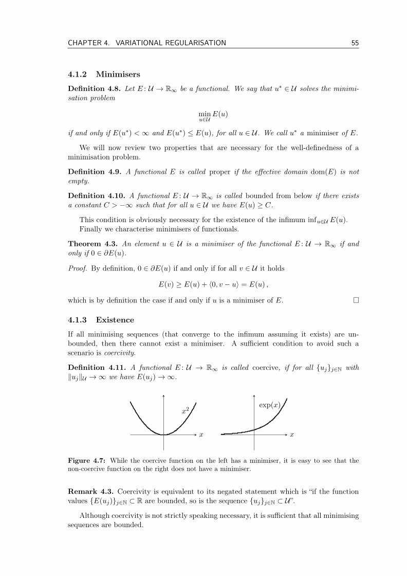
CHAPTER 4. VARIATIONAL REGULARISATION 55
4.1.2 Minimisers
Definition 4.8. Let E : U → R∞ be a functional. We say that u∗ ∈ U solves the minimi-sation problem
minu∈U
E(u)
if and only if E(u∗) <∞ and E(u∗) ≤ E(u), for all u ∈ U . We call u∗ a minimiser of E.
We will now review two properties that are necessary for the well-definedness of aminimisation problem.
Definition 4.9. A functional E is called proper if the effective domain dom(E) is notempty.
Definition 4.10. A functional E : U → R∞ is called bounded from below if there existsa constant C > −∞ such that for all u ∈ U we have E(u) ≥ C.
This condition is obviously necessary for the existence of the infimum infu∈U E(u).Finally we characterise minimisers of functionals.
Theorem 4.3. An element u ∈ U is a minimiser of the functional E : U → R∞ if andonly if 0 ∈ ∂E(u).
Proof. By definition, 0 ∈ ∂E(u) if and only if for all v ∈ U it holds
E(v) ≥ E(u) + 〈0, v − u〉 = E(u) ,
which is by definition the case if and only if u is a minimiser of E.
4.1.3 Existence
If all minimising sequences (that converge to the infimum assuming it exists) are un-bounded, then there cannot exist a minimiser. A sufficient condition to avoid such ascenario is coercivity.
Definition 4.11. A functional E : U → R∞ is called coercive, if for all ujj∈N with‖uj‖U →∞ we have E(uj)→∞.
x2
x
exp(x)
x
Figure 4.7: While the coercive function on the left has a minimiser, it is easy to see that thenon-coercive function on the right does not have a minimiser.
Remark 4.3. Coercivity is equivalent to its negated statement which is “if the functionvalues E(uj)j∈N ⊂ R are bounded, so is the sequence ujj∈N ⊂ U”.
Although coercivity is not strictly speaking necessary, it is sufficient that all minimisingsequences are bounded.
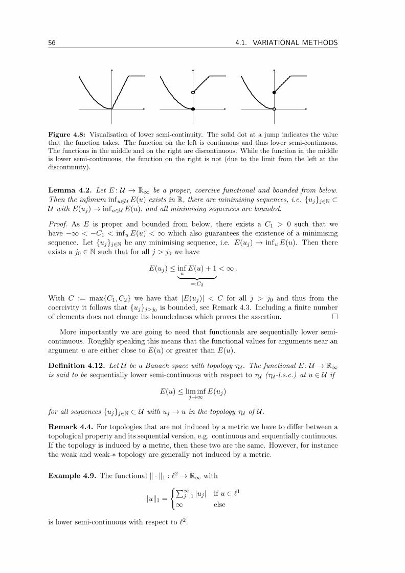
56 4.1. VARIATIONAL METHODS
Figure 4.8: Visualisation of lower semi-continuity. The solid dot at a jump indicates the valuethat the function takes. The function on the left is continuous and thus lower semi-continuous.The functions in the middle and on the right are discontinuous. While the function in the middleis lower semi-continuous, the function on the right is not (due to the limit from the left at thediscontinuity).
Lemma 4.2. Let E : U → R∞ be a proper, coercive functional and bounded from below.Then the infimum infu∈U E(u) exists in R, there are minimising sequences, i.e. ujj∈N ⊂U with E(uj)→ infu∈U E(u), and all minimising sequences are bounded.
Proof. As E is proper and bounded from below, there exists a C1 > 0 such that wehave −∞ < −C1 < infuE(u) < ∞ which also guarantees the existence of a minimisingsequence. Let ujj∈N be any minimising sequence, i.e. E(uj) → infuE(u). Then thereexists a j0 ∈ N such that for all j > j0 we have
E(uj) ≤ infuE(u) + 1︸ ︷︷ ︸=:C2
<∞ .
With C := maxC1, C2 we have that |E(uj)| < C for all j > j0 and thus from thecoercivity it follows that ujj>j0 is bounded, see Remark 4.3. Including a finite numberof elements does not change its boundedness which proves the assertion.
More importantly we are going to need that functionals are sequentially lower semi-continuous. Roughly speaking this means that the functional values for arguments near anargument u are either close to E(u) or greater than E(u).
Definition 4.12. Let U be a Banach space with topology τU . The functional E : U → R∞is said to be sequentially lower semi-continuous with respect to τU (τU -l.s.c.) at u ∈ U if
E(u) ≤ lim infj→∞
E(uj)
for all sequences ujj∈N ⊂ U with uj → u in the topology τU of U .
Remark 4.4. For topologies that are not induced by a metric we have to differ between atopological property and its sequential version, e.g. continuous and sequentially continuous.If the topology is induced by a metric, then these two are the same. However, for instancethe weak and weak-∗ topology are generally not induced by a metric.
Example 4.9. The functional ‖ · ‖1 : `2 → R∞ with
‖u‖1 =
∑∞j=1 |uj | if u ∈ `1
∞ else
is lower semi-continuous with respect to `2.

CHAPTER 4. VARIATIONAL REGULARISATION 57
Proof. Let ujj∈N ⊂ `2 be a convergent sequence with uj → u ∈ `2. As strong convergenceimplies weak convergence, we have with δk : `2 → R, 〈δk, v〉 = vk that for all k ∈ N that
ujk = 〈δk, uj〉 → 〈δk, u〉 = uk .
The assertion follows then with Fatou’s lemma
‖u‖1 =
∞∑k=1
|uk| =∞∑k=1
limj→∞
|ujk| ≤ lim infj→∞
∞∑k=1
|ujk| = lim infj→∞
‖uj‖1 .
Note that it is not clear whether both the left and the right hand side are finite.
Example 4.10. Let Ω ⊂ Rn be open and bounded. Then, the total variation is lowersemi-continuous with respect to L1.
Proof. Recall that the total variation was defined by means of the test functions
D(Ω,Rn) :=ϕ ∈ C∞0 (Ω;Rn)
∣∣∣ supx∈Ω‖ϕ(x)‖2 ≤ 1
as
TV(u) = supϕ∈D(Ω,Rn)
∫Ωu(x) divϕ(x) dx .
Let ujj∈N ⊂ BV(Ω) be a sequence converging in L1(Ω) with uj → u in L1(Ω). Then forany test function ϕ ∈ D(Ω,Rn) there is∫
Ω[u(x)− uj(x)] divϕ(x)dx ≤
∫Ω|u(x)− uj(x)|dx︸ ︷︷ ︸=‖u−uj‖L1→0
supx∈Ω|divϕ(x)|︸ ︷︷ ︸<∞
→ 0
and thus ∫Ωu(x) divϕ(x)dx = lim inf
j→∞
∫Ωuj(x) divϕ(x)dx ≤ lim inf
j→∞TV(uj) .
Taking the supremum over all test functions shows the assertion. Note that again the leftand right hand side may not be finite.
We have now all ingredients in place for a positive answer about the existence of min-imisers also known as the “direct method” or “fundamental theorem of optimisation”.
Theorem 4.4 (“Direct method”, David Hilbert, around 1900). Let U be a Banach spaceand τU a topology (not necessarily the one induced by the norm) on U such that boundedsequences have τU -convergent subsequences. Let E : U → R∞ be proper, bounded frombelow, coercive and τU -l.s.c. Then E has a minimiser.
Proof. From Lemma 4.2 we know that infu∈U E(u) is finite, minimising sequences existand that they are bounded. Let ujj∈N ∈ U be a minimising sequence. Thus, fromthe assumption on the topology τU there exists a subsequence ujkk∈N and u∗ ∈ U withujk
τU→ u∗ for k →∞. From the sequential lower semi-continuity of E we obtain
E(u∗) ≤ lim infk→∞
E(ujk) = limj→∞
E(uj) = infu∈U
E(u) <∞ ,
which shows that E(u∗) <∞ and E(u∗) ≤ E(u) for all u ∈ U ; thus u∗ minimises E.
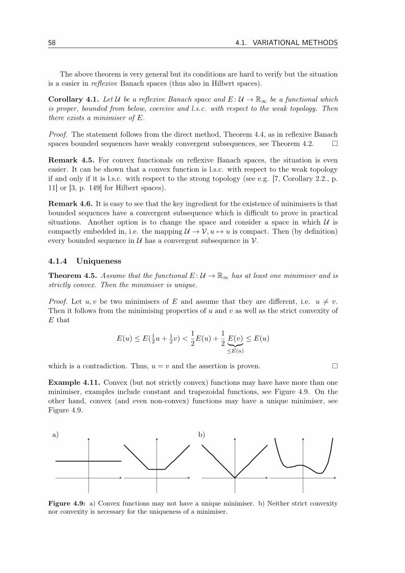
58 4.1. VARIATIONAL METHODS
The above theorem is very general but its conditions are hard to verify but the situationis a easier in reflexive Banach spaces (thus also in Hilbert spaces).
Corollary 4.1. Let U be a reflexive Banach space and E : U → R∞ be a functional whichis proper, bounded from below, coercive and l.s.c. with respect to the weak topology. Thenthere exists a minimiser of E.
Proof. The statement follows from the direct method, Theorem 4.4, as in reflexive Banachspaces bounded sequences have weakly convergent subsequences, see Theorem 4.2.
Remark 4.5. For convex functionals on reflexive Banach spaces, the situation is eveneasier. It can be shown that a convex function is l.s.c. with respect to the weak topologyif and only if it is l.s.c. with respect to the strong topology (see e.g. [7, Corollary 2.2., p.11] or [3, p. 149] for Hilbert spaces).
Remark 4.6. It is easy to see that the key ingredient for the existence of minimisers is thatbounded sequences have a convergent subsequence which is difficult to prove in practicalsituations. Another option is to change the space and consider a space in which U iscompactly embedded in, i.e. the mapping U → V, u 7→ u is compact. Then (by definition)every bounded sequence in U has a convergent subsequence in V.
4.1.4 Uniqueness
Theorem 4.5. Assume that the functional E : U → R∞ has at least one minimiser and isstrictly convex. Then the minimiser is unique.
Proof. Let u, v be two minimisers of E and assume that they are different, i.e. u 6= v.Then it follows from the minimising properties of u and v as well as the strict convexity ofE that
E(u) ≤ E(12u+ 1
2v) <1
2E(u) +
1
2E(v)︸ ︷︷ ︸≤E(u)
≤ E(u)
which is a contradiction. Thus, u = v and the assertion is proven.
Example 4.11. Convex (but not strictly convex) functions may have have more than oneminimiser, examples include constant and trapezoidal functions, see Figure 4.9. On theother hand, convex (and even non-convex) functions may have a unique minimiser, seeFigure 4.9.
a) b)
Figure 4.9: a) Convex functions may not have a unique minimiser. b) Neither strict convexitynor convexity is necessary for the uniqueness of a minimiser.

CHAPTER 4. VARIATIONAL REGULARISATION 59
4.2 Well-posedness and regularisation properties
The aim of this section is to have a detailed look at the model Rα : V → U with
Rαf := arg minu∈U
Φα,f (u) :=
1
2‖Ku− f‖2V + αJ(u)
. (4.5)
We will establish conditions on the spaces U ,V, the functional J and the operator K underwhich a minimiser exists and is unique and therefore the mapping Rα is well-defined.We will analyse the continuity of the mapping Rα which means that the solution dependscontinuous on the data and thus can handle small variations due to noise. We also show thatthere are parameter choice rules that make Rα a convergent regularisation in a modifiedsense (that we will define later) and prove convergence rates under a source condition.
4.2.1 Existence and uniqueness
Existence
Lemma 4.3. Let U be a Banach space and τU a topology on it. Let E : U → R andF : U → R∞ be proper functionals that are both τU -l.s.c. and bounded from below. ThenE + F : U → R∞ is proper, τU -l.s.c. and bounded from below.
Proof. First of all, as F is proper, there exists u ∈ U such that F (u) <∞ and as E(u) <∞it is clear that (E + F )(u) <∞ which shows that E + F is proper.
Second, for all u ∈ U we have from the boundedness from below of E and F thatE(u) ≥ C1 and F (u) ≥ C2 and thus,
(E + F )(u) = E(u) + F (u) ≥ C1 + C2 > −∞ .
Finally, let ujj∈N ⊂ U be a sequence and u ∈ U with uj → u in τU . Then by τU -l.s.c.we have that
(E + F )(u) ≤ lim infj→∞
E(uj) + lim infj→∞
F (uj)
≤ lim infj→∞
(E(uj) + F (uj)) = lim infj→∞
(E + F )(uj)
which shows that E + F is τU -l.s.c. and all assertions are proven.
Lemma 4.4. Let U be a Banach space and E,F : U → R∞ be functionals. Let E becoercive and F be bounded from below, then E + F is coercive.
Proof. From the boundedness from below of F , there exists a constant C ∈ R such thatF (u) > C for all u ∈ U . Thus we see that
(E + F )(u) = E(u) + F (u) ≥ E(u) + C →∞as ‖u‖U →∞ which proves that E + F is coercive.
In many situations of interest, the lemma above does not apply because the coercivitycomes jointly from the data term and the prior as we will see in the following example.
Example 4.12. Let Ω ⊂ Rn be bounded and consider total variation regularisation, i.e.J = TV and U = BV(Ω). One can easily see that constant functions have zero totalvariation, i.e. TV(u) = 0, for all u ≡ c, c ∈ R. Notice that this implies that J is notcoercive on the whole space U as uj(x) = j/|Ω|, |Ω| :=
∫Ω 1 dx defines a sequence such that
‖uj‖L1 = j and TV(uj) = 0. However, we can make use of a Poincaré–Wirtinger inequalityfor BV.

60 4.2. WELL-POSEDNESS AND REGULARISATION PROPERTIES
Proposition 4.1 ([8, p. 24]). Let Ω ⊂ Rn be a Lipschitz domain (non-empty, open,connected and bounded with Lipschitz boundary). There exists a constant C > 0 such thatfor all u ∈ BV(Ω) the Poincaré–Wirtinger type inequality is satisfied
‖u− uΩ‖L1 ≤ C TV(u)
where uΩ := 1|Ω|∫
Ω u(x)dx is the mean-value of u over Ω.
Continuation of Example 4.12. Let Ω now fulfil the conditions of Proposition 4.1.Furthermore, let p0 ∈ U∗ with
〈p0, u〉 := uΩ =1
|Ω|
∫Ωu(x)dx
and denote the space of zero-mean functions by U0 := u ∈ U |u ∈ N (p0). By thePoincaré–Wirtinger inequality it is clear that the total variation is coercive on U0 and thedata term has to make sure that the functional Φα,f is coercive on the whole space U .As we will see in the next, Lemma 4.5, the condition 1 6∈ N (K) is sufficient to guaranteecoercivity in this scenario. This will follow from a more general result.
Lemma 4.5. Let U ,V be Banach spaces, K ∈ L(U ,V), J : U → [0,∞] and f ∈ V. Letp0 ∈ U∗, u0 ∈ U , 〈p0, u0〉 = 1,
U0 := u ∈ U | u ∈ N (p0)
so that u0 6∈ N (K) and J is coercive on U0 in the sense that
‖u− 〈p0, u〉u0‖U →∞ implies J(u)→∞ .
Then the variational regularisation functional Φα,f defined by (4.5) is coercive.
Proof. Any u ∈ U can be decomposed into
u = v + w
where v := u− 〈p0, u〉u0 ∈ U0 and w := 〈p0, u〉u0 ∈ span(u0).Now, let ujj∈N ⊂ U be a sequence with ‖uj‖U →∞. On the one hand, if ‖vj‖U →∞,
then by the coercivity of J on U0 and the boundedness from below of the data term, wehave that Φα,f (uj)→∞.
On the other hand, if ‖vj‖U < C for some C > 0, then from
‖uj‖U ≤ ‖vj‖U + ‖wj‖U < C + |〈p0, uj〉|‖u0‖U
it follows that |〈p0, uj〉| → ∞. Therefore,
‖Kuj − f‖V = ‖K(vj + wj)− f‖V≥ ‖Kwj‖V − ‖Kvj − f‖V≥ ‖Ku0‖V︸ ︷︷ ︸
>0
|〈p0, uj〉|︸ ︷︷ ︸
→∞
−‖K‖C − ‖f‖V︸ ︷︷ ︸constant
→∞
and thus Φα,f (uj)→∞ as the regularisation functional J is bounded from below.

CHAPTER 4. VARIATIONAL REGULARISATION 61
Remark 4.7. A natural question here is whether the coercivity can also come completelyfrom the data term D(u) = 1
2‖Ku− f‖2V . On the one hand if K is not injective, then thekernel is non-trivial, thus we cannot expect the data term to be coercive.
On the other hand, even if K was injective we cannot expect coercivity in general.Assume that the data term D was coercive, U a Hilbert space, the topologies τU , τV theweak topologies on U ,V, f ∈ R(K) \ R(K) and D τU -l.s.c. (e.g. see Lemma 4.6). Thenwe can apply the direct method on the data term D and would prove the existence of aminimiser. This is by definition a least squares solution; a contradiction to Lemma 2.2.
The remark will be illustrated by the following example.
Example 4.13. Let us consider the Example 2.1 again where the operator was K : `2 →`2, (Ku)j := uj/j and the data f ∈ `2 with fj := 1/j. Then the ukk∈N ⊂ `2 with
ukj :=
1 j ≤ k0 else
defines a sequence Kukk∈N with Kuk → f in `2.Note that K is injective and ukk∈N is a minimising sequence of the data term, i.e.
‖Kuk − f‖`2 → 0. However, as ‖uk‖`2 = k the sequence ukk∈N is unbounded and thusu 7→ ‖Ku− f‖`2 cannot be coercive.
Lemma 4.6. Let U and V be Banach spaces with topologies τU and τV . Moreover, let thenorm on V be τV-l.s.c., the operator K : U → V be sequentially continuous with respect tothe topologies τU and τV and let fjj∈N ⊂ V be convergent in τV with fj → f ∈ V. Thenfor any τU -convergent sequence ujj∈N ⊂ U with uj → u ∈ U with respect to τU , we have
1
2‖Ku− f‖2V ≤ lim inf
j→∞
1
2‖Kuj − fj‖2V .
In particular, if fj ≡ f , then D : U → R, u 7→ 12‖Ku− f‖2V is τU -l.s.c.
Proof. Let ujj∈N be a τU -convergent sequence and denote its limit by u ∈ U , i.e. uj → uin τU . Because K is continuous with respect to τU and τV we have that Kuj → Ku in τVand thus Kuj − fj → Ku − f in τV . Thus, the assertion follows from the τV -l.s.c. of thenorm.
Remark 4.8. If the topologies τU and τV are the weak topologies, then the situation ismuch simpler as continuity in the strong topologies implies continuity in the weak topologies[5, chapter IV.3]. Thus the assumptions of Lemma 4.6 are met if K is continuous.
Note that the norm is convex (will be proven in what follows) such that weak-l.s.c. isequivalent to l.s.c.
Now we are in a position to state sufficient assumptions for the existence of minimisers.
Assumption 4.1. Sufficient assumptions for the existence of minimisers of Φα,f are:
(a) The Banach space U and Hilbert space V are associated with the topologies τU andτV . The pair (U , τU ) has the property that bounded sequences have τU -convergentsubsequences. Moreover, the norm on V is τV-l.s.c.
(b) The operator K : U → V is linear and sequentially continuous with respect to thetopologies τU and τV .
62 4.2. WELL-POSEDNESS AND REGULARISATION PROPERTIES
(c) The functional J : U → [0,∞] is proper and τU -l.s.c.
(d) Either J is coercive or the pair (K,J) fulfil the assumptions of Lemma 4.5.
Theorem 4.6. Let the Assumptions 4.1 hold and let f ∈ V, α > 0. Then the variationalregularisation functional Φα,f defined by (4.5) has a minimiser.
Proof. It follows from the assumptions by Lemmata 4.3 and 4.6 that Φα,f is proper, τU -l.s.c.and bounded from below. Moreover, from Lemmata 4.4 or 4.5 (depending on assumption4.1 (d)) Φα,f is coercive. Then from the direct method, Theorem 4.4, it follows that thereexists a minimiser.
Uniqueness
Lemma 4.7. Let U be a Banach space and and V a Hilbert space. Furthermore, let K ∈L(U ,V), f ∈ V and D : U → R∞ be defined as D(u) := 1
2‖Ku − f‖2V . Then D is convex.Furthermore, D is strictly convex if and only if K is injective.
Proof. Let λ ∈ (0, 1) and u, v ∈ U with u 6= v.Long and straightforward calculations (good exercise) yield
D(λu+ (1− λ)v) = λD(u) + (1− λ)D(v)− λ(1− λ)
2‖K(u− v)‖2V︸ ︷︷ ︸≥0
,
which shows that D is convex.Note that ‖K(u − v)‖V > 0 if K is injective and u 6= v. On the other hand, if K
is not injective, then we can find u, v ∈ U with u 6= v so that u − v ∈ N (K) and thus‖K(u− v)‖V = 0 which shows that D is not strictly convex.
Remark 4.9. The lemma is in general not true if V is a Banach space. As an example,consider K = I, f = 0, V = R2 with ‖ · ‖1 as a norm. Then D is not strictly convex.
Example 4.14. Let U be continuously embedded into the Hilbert space Z (in symbolsU → Z), i.e. there exists a constant C > 0 such that for all u ∈ U there is ‖u‖Z ≤ C‖u‖U .Furthermore, let β > 0 and J be convex. Then the functional Φα,f + β
2 ‖ · ‖2Z is alwaysstrictly convex independent of K.
Consider the product space V × Z which is a Hilbert space with the inner product
〈(v1, z1), (v2, z2)〉V×Z := 〈v1, v2〉V + 〈z1, z2〉Z .
Then we can rewrite 12‖Ku− f‖2V + β
2 ‖u‖2Z as
1
2
∥∥∥∥( K√βI
)u−
(f0
)∥∥∥∥2
V×Z=
1
2‖Ku− f‖2V
where the modified operator K is injective. Therefore, adding the term β2 ‖u‖2Z can be seen
as a regularisation of the linear operator K directly.
Theorem 4.7. Let the Assumptions 4.1 hold and let J be convex. Moreover, let eitherK be injective or J be strictly convex. Then for any f ∈ V and α > 0 the variationalregularisation model Rα is well-defined (there exists a unique minimiser of the functionalΦα,f defined by (4.5)).

CHAPTER 4. VARIATIONAL REGULARISATION 63
Proof. Existence follows immediately from Theorem 4.6. For the uniqueness, notice thatboth 1
2‖Ku− f‖2V and αJ are convex and either of them is strictly convex by assumption,see Lemma 4.7. Thus by Lemma 4.1 the whole functional Φα,f is strictly convex andtherefore the minimiser is unique, see Theorem 4.5.
Example 4.15. Let α, β > 0,K ∈ L(`2, `2) and consider the elastic net variational regu-larisation model 1
2‖Ku− f‖2`2 + αJ(u) with
J(u) =
‖u‖1 + β
2 ‖u‖22 if u ∈ `1∞ else
.
We check the assumptions of Theorem 4.7 in this setting to conclude that Rα is well-defined.Let U ,V = `2 and as these are Hilbert spaces we choose the topologies τU , τV to be
both the weak topology on `2. By Remark 4.8 the Assumptions 4.1 (a) and (b) are fulfilledand we can show lower semi-continuity in the strong topology rather than the weak one.It is easy to see that the prior J is strictly convex, proper and coercive. It remains to showthat J is lower semi-continuous with respect to `2. The squared `2-norm is continuous,thus lower semi-continuous and the lower semi-continuity of the `1-norm has been provenin Example 4.9 such that the elastic net is lower semi-continuous by Lemma 4.3. As it isconvex, l.s.c. is equivalent to weak-l.s.c. and all assumptions of Theorem 4.7 hold.
For the example of the total variation we need to have some knowledge about compactembeddings of BV(Ω).
Theorem 4.8 (Rellich-Kandrachov, [1, p. 168]). Let Ω ⊂ Rn be a Lipschitz domain andeither
n > mp and p∗ := np/(n−mp)or n ≤ mp and p∗ :=∞ .
Then the embedding Hm,p(Ω) → Lq(Ω) is continuous if 1 ≤ q ≤ p∗ and compact if inaddition q < p∗.
Due to approximations of u ∈ BV(Ω) by smooth functions the Rellich-KandrachovTheorem (for m = 1, p = 1) gives us compactness for BV(Ω).
Corollary 4.2 ([8, p. 17]). For any Lipschitz domain Ω ⊂ Rn the embedding
BV(Ω)→ L1(Ω)
is compact.
Example 4.16. Let Ω ⊂ Rn be a Lipschitz domain, α > 0,K ∈ L(L1(Ω), L2(Ω)) beinjective and consider the total variation regularised model Rα : L2(Ω) → BV(Ω), Rαf :=arg minu∈BV(Ω) Φα,f (u) with
Φα,f (u) =1
2‖Ku− f‖2L2 + αTV(u) .
This time we are neither in a Hilbert nor in a reflexive Banach space setting but fromCorollary 4.2 we see that BV(Ω) is compactly embedded in L1(Ω). Thus every sequencebounded in BV(Ω) has a convergent subsequence in L1(Ω).
Let τU and τV be the topologies induced by the L1-norm, respectively L2-norm. It isclear that the assumptions on the spaces and topologies are met. The lower semi-continuityof TV with respect to L1 was shown in Example 4.10. Moreover, it can be shown that TVis proper and convex. The injectivity of K implies that 1 6∈ N (K). From Example 4.12and 1 6∈ N (K) it follows that Φα,f is coercive. Thus, a minimiser exists. The injectivity ofthe operator K guarantees strict convexity and therefore the uniqueness of the minimiser.

64 4.2. WELL-POSEDNESS AND REGULARISATION PROPERTIES
4.2.2 Continuity
We have seen that under some assumptions the variational regularisation Rα is well-defined(solutions exists and are unique). In this section we show that variational regularisationis continuous with respect to the data, i.e. small variations in the data do not lead toarbitrary large distortions in the solution. To establish the main result we have to proveauxiliary lemmata.
Lemma 4.8. Let V be a normed space. For all f, g ∈ V there is
‖f + g‖2V ≤ 2‖f‖2V + 2‖g‖2V .
Proof. For any f, g ∈ V we have with the monotonicity of [0,∞)→ [0,∞), x 7→ x2 that
‖f + g‖2V ≤(‖f‖V + ‖g‖V
)2
= ‖f‖2V + 2‖f‖V‖g‖V + ‖g‖2V .
We complete the proof with the observation that 2ab ≤ a2 + b2 for all a, b ∈ R.
Lemma 4.9. Let U ,V be normed spaces. For all u ∈ U and f, g ∈ V there is
Φα,f (u) ≤ 2Φα,g(u) + ‖f − g‖2V .
Proof. Using Lemma 4.8 and J(u) ≥ 0, we have
Φα,f (u) =1
2‖Ku− f‖2V + αJ(u) =
1
2‖Ku− g + (g − f)‖2V + αJ(u)
≤ ‖Ku− g‖2V + ‖g − f‖2V + 2αJ(u)
= 2
(1
2‖Ku− g‖2U + αJ(u)
)+ ‖f − g‖2V
= 2Φα,g(u) + ‖f − g‖2V .
Theorem 4.9 (Continuity). Assume the setting of Theorem 4.7 that guarantees the ex-istence and uniqueness of minimisers of Φα,f (u) := 1
2‖Ku − f‖2V + αJ(u) for any f ∈ Vand α > 0. Moreover, let the topology τV on V be weaker than the norm topology in thesense that convergence in norm implies convergence in τV . Then, the mapping Rα : V →U , Rαf := arg minu∈U Φα,f (u) is sequentially strong-τU continuous, i.e. for all sequencesfjj∈N ⊂ V with fj → f we have
Rαfj → Rαf in τU .
Moreover, the function values of the regulariser converge, i.e. J(Rαfj)→ J(Rαf).
Proof. Let fjj∈N ⊂ V be a convergent sequence with fj → f and let uj := Rαfj be theminimiser of Φα,fj .
We first show that Φα,f (uj)j∈N ⊂ R is bounded. To see this, as J is proper, thereexists u ∈ U such that J(u) < ∞ and we denote C := 2‖Ku‖2V + 2αJ(u). With Lemmaand 4.9 and the minimising property of uj we have that
Φα,f (uj) ≤ 2Φα,fj (uj) + ‖f − fj‖2V≤ 2Φα,fj (u) + ‖f − fj‖2V = ‖Ku− fj‖2V + 2αJ(u) + ‖f − fj‖2V
CHAPTER 4. VARIATIONAL REGULARISATION 65
With Lemma 4.8 we can further estimate
‖Ku− fj‖2V + 2αJ(u) + ‖f − fj‖2V ≤ 2‖Ku‖2V + 2‖fj‖2V + 2αJ(u) + ‖f − fj‖2V≤ 2‖fj‖2V + ‖f − fj‖2V + C .
As fj converges to f , there exists a j0 ∈ N such that for all j > j0 there is
Φα,f (uj) ≤ 2 ‖fj‖2V︸ ︷︷ ︸‖f‖2V+1
+ ‖f − fj‖2V︸ ︷︷ ︸≤1
+C ≤ 2‖f‖2V + C + 3 <∞ .
By the coercivity of Φα,f we know that the sequence ujj∈N ⊂ U is bounded, see Remark4.3. Thus there exist τU -convergent subsequences and let ujkk∈N ⊂ U be any one ofthose. We denote its limit by u∗ ∈ U , i.e. ujk → u∗ in τU .
From Lemma 4.6 and as J is τU -l.s.c. we have that
1
2‖Ku∗ − f‖2V ≤ lim inf
k→∞
1
2‖Kujk − fjk‖2V and J(u∗) ≤ lim inf
k→∞J(ujk) (4.6)
and therefore
Φα,f (u∗) =1
2‖Ku∗ − f‖2V + αJ(u∗)
≤ lim infk→∞
1
2‖Kujk − fjk‖2V + α lim inf
k→∞J(ujk)
≤ lim infk→∞
(1
2‖Kujk − fjk‖2V + αJ(ujk)
)= lim inf
k→∞Φα,fjk
(ujk) .
With the minimising property of ujk we arrive at
Φα,f (u∗) ≤ lim infk→∞
Φα,fjk(ujk)
≤ lim infk→∞
Φα,fjk(u) = lim
k→∞Φα,fjk
(u) = Φα,f (u)(4.7)
for all u ∈ U . In particular, this holds for u = Rαf . Thus, as the minimiser of Φα,f
is unique, we have that u∗ = Rαf . Repeating the same arguments as above for anysubsequence of ujj∈N instead of ujj∈N, we see that every subsequence has a convergentsubsequence that converges to Rαf in τU . Thus, ujj∈N is convergent in τU and we haveuj → Rαf in τU and the first assertion is proven.
Moreover, from (4.7) it follows with uj → Rαf in τU that
limj→∞
Φα,fj (uj) = Φα,f (Rαf) .
and therefore
lim supj→∞
αJ(uj) = lim supj→∞
(1
2‖Kuj − fj‖2V + αJ(uj)−
1
2‖Kuj − fj‖2V
)≤ lim sup
j→∞
(1
2‖Kuj − fj‖2V + αJ(uj)
)︸ ︷︷ ︸
=limj→∞ Φα,fj (uj)=Φα,f (Rαf)
+ lim supj→∞
(−1
2‖Kuj − fj‖2V
)
=1
2‖KRαf − f‖2V + αJ(Rαf)− lim inf
j→∞
1
2‖Kuj − fj‖2V︸ ︷︷ ︸
≤− 12‖KRαf−f‖2V by (4.6)
≤ αJ(Rαf) .

66 4.2. WELL-POSEDNESS AND REGULARISATION PROPERTIES
The τU -l.s.c. of J proves the second assertion
lim supj→∞
αJ(uj) ≤ αJ(Rαf) ≤ lim infj→∞
αJ(uj) .
Remark 4.10. In the theorem above we could only prove convergence in τU . If J statisfiesthe Radon-Riesz property with respect to the topology τU , i.e. uj → u in τU and J(uj)→J(u) imply ‖uj − u‖U → 0, then the convergence is in the norm topology. An example ofa functional satisfying the Radon-Riesz property is ‖ · ‖pLp / ‖ · ‖p`p with 1 < p < ∞ if theunderlying space is Lp / `p and τU being the weak topology.
4.2.3 Convergent regularisation
Note that variational regularisation for general J is not necessarily a regularisation in thesense of Definition 3.1, as we cannot expect Rαf = arg minu∈U Φα,f (u) → u† for α → 0where u† is the minimal norm solution. However, we can generalise Definition 2.1 of aminimal norm solution (and a least squares solution) to justify calling Rα a regularisation.
Definition 4.13. Let U and V be normed spaces and f ∈ V. We call u ∈ U a least squaressolution of the inverse problem (1.1), if
u ∈ arg minv∈U‖Kv − f‖V (4.8)
As in the case of Hilbert spaces, we denote by L the set of all least squares solutions (itmight be empty). Furthermore, we call u† ∈ U a J-minimising solution of the inverseproblem (1.1), if
u† ∈ arg minu∈L
J(u) . (4.9)
Remark 4.11. If V is a Hilbert space (as in our setting in Assumption 4.1), then mostof the statements from Chapter 2 about least squares solutions still hold. In particularLemma 2.2, which states that L 6= ∅ if and only if f ∈ R(K) ⊕ R(K)⊥. However, theminimal norm solution (J-minimising solution for J = ‖ ·‖U ) may not be unique any more.
Lemma 4.10. Let U be a vector space and E : U → R∞ a convex functional. Then the setof all minimisers S, i.e.
S := arg minu∈U
E(u) ,
is convex.
Proof. For any u, v ∈ S, u 6= v and λ ∈ (0, 1), it is easy to see that
E(λu+ (1− λ)v) ≤ λE(u) + (1− λ)E(v)
≤ λ infw∈U
E(w) + (1− λ) infw∈U
E(w) = infw∈U
E(w)
which shows that λu+ (1− λ)v ∈ S and thus S is convex.
Corollary 4.3. Let U and V be normed spaces, f ∈ V and K : U → V be linear. Then theset of least squares solutions L is convex.
Proof. One can show that u 7→ ‖Ku− f‖V is convex so that the lemma applies.

CHAPTER 4. VARIATIONAL REGULARISATION 67
Lemma 4.11. Let U be a Banach space, V be a Hilbert space, f ∈ V and K : U → V belinear and injective. Then the set of least squares solutions L is at most a singleton.
Proof. Assume that least squares solutions exist which are equivalently characterised by
u ∈ arg minv∈U
D(v) :=
1
2‖Kv − f‖2V
. (4.10)
From Lemma 4.7 we know that D is strictly convex and thus by Theorem 4.5 the minimiseris unique.
Proposition 4.2. Let the assumptions of Theorem 4.7 hold and f ∈ R(K) ⊕ R(K)⊥.Then a J-minimising solution exists and is unique.
Proof. By Remark 4.11, the condition f ∈ R(K)⊕R(K)⊥ guarantees the existence of leastsquares solutions, i.e. L 6= ∅. For the existence of J-minimising solutions via the directmethod, Theorem 4.4, we see that only the coercivity on L may not be guaranteed by theassumptions.
If J is coercive, then it is obviously also coercive on L. If J is only coercive on U0 (seeLemma 4.5 for a definition), then a similar calculation as in the proof of Lemma 4.5 showsthat for any sequence ujj∈N ⊂ L we have with
uj = uj − 〈p0, uj〉u0︸ ︷︷ ︸
=:vj
+ 〈p0, uj〉u0︸ ︷︷ ︸
=:wj
that
‖f‖V = ‖K0− f‖V ≥ ‖Kuj − f‖V= ‖K(vj + wj)− f‖V≥ ‖Kwj‖V − ‖f −Kvj‖V > ‖Ku0‖V |〈p0, u
j〉| − ‖f‖V − ‖K‖‖vj‖V .
Let ujj∈N ⊂ L with ‖uj‖U → ∞. If ‖vj‖V was bounded, then so would be |〈p0, uj〉|
which contradicts the unboundedness of ujj∈N. Thus
‖vj‖U = ‖uj − 〈p0, uj〉‖U →∞
and J(uj)→∞ by the coercivity of J on U0.For the uniqueness, either J is strictly convex (and thus a minimiser is unique) or K
is injective and only one least squares solution exists.
Definition 4.14 (Regularisation). Let U ,V be Banach spaces, τU a topology on U , f ∈ Vand K ∈ L(U ,V). Moreover, let u† be the J-minimising solution (assuming it exists andis unique). We call the family of operators Rαα>0, Rα : V → U a regularisation (withrespect to τU) of the inverse problem (1.1), if Rα is sequentially strong-τU continuous forall α > 0 and
Rαf → u† in τU as α→ 0.
Theorem 4.10. Let the assumptions of Theorem 4.7 hold and assume (for simplicity) thatthe clean data is in the range, i.e. f ∈ R(K), thus the J-minimising solution u† exists andis unique. Moreover, assume that the topology τV is weaker than the norm topology on V.Let α : (0,∞)→ (0,∞) be a parameter choice rule with
α(δ)→ 0, andδ2
α(δ)→ 0 as δ → 0 .

68 4.2. WELL-POSEDNESS AND REGULARISATION PROPERTIES
Let δjj∈N ⊂ [0,∞) be a sequence of noise levels with δj → 0 and fjj∈N ⊂ V be asequence of noisy observations with ‖f − fj‖V ≤ δj. Set αj := α(δj) and let ujj∈N be thesequence of minimisers of Φαj ,fj , i.e. uj := Rαjfj.
Then uj → u† in τU and J(uj)→ J(u†). In particular, Rα is a regularisation.
Proof. From minimising property of uj and Ku† = f , it follows that
0 ≤ 1
2‖Kuj − fj‖2V + αjJ(uj)
≤ 1
2‖Ku† − fj‖2V + αjJ(u†)
=1
2‖f − fj‖2V + αjJ(u†) ≤
δ2j
2+ αjJ(u†)→ 0
(4.11)
as j →∞ (δj , αj → 0). In particular limj→∞ ‖Kuj − fj‖V = 0, and then
‖Kuj − f‖V ≤ ‖Kuj − fj‖V + ‖fj − f‖V ≤ ‖Kuj − fj‖V + δj → 0 . (4.12)
Similarly, we see from (4.11) that
lim supj→∞
J(uj) ≤ lim supj→∞
δ2j
2αj+ J(u†) = J(u†) . (4.13)
Let α+ := maxj∈N αj be the largest regularisation parameter (which exists as αj → 0),then
lim supj→∞
Φα+,f (uj) = lim supj→∞
(1
2‖Kuj − f‖2V + α+J(uj)
)≤ lim sup
j→∞
1
2‖Kuj − f‖2V︸ ︷︷ ︸=0
+ lim supj→∞
α+J(uj)︸ ︷︷ ︸≤α+J(u†)
≤ α+J(u†) =: C <∞
This shows that there exists a j0 ∈ N such that for all j ≥ j0 we have that Φα+,f (uj) ≤ C+1.From the coercivity of Φα+,f it follows that ujj∈N is bounded and therefore has a
τU -convergent subsequence ujkk∈N with ujk → u in τU . By the continuity of K withrespect to τU and τV we have that Kujk → Ku in τV . With the τV -l.s.c. of the norm of Vwe conclude that Ku = f as
‖Ku− f‖V ≤ lim infk→∞
‖Kujk − f‖V = 0 .
Thus u is a least squares solution.From (4.13) and the τU -l.s.c. of J we have that
J(u) ≤ lim infk→∞
J(ujk) ≤ lim supk→∞
J(ujk) ≤ J(u†) ≤ J(u) (4.14)
for all u ∈ U . Thus, u is a J-minimising solution, which implies by its uniqueness thatu = u†. Moreover, from (4.14) we deduce J(ujk)→ J(u†).
As in the proof of Theorem 4.9, all arguments can be applied to any subsequence ofujj∈N, which shows that uj → u† in τU and J(uj)→ J(u†).
Remark 4.12. Similar to the stability we can get strong convergence if J satisfies theRadon-Riesz property.
CHAPTER 4. VARIATIONAL REGULARISATION 69
4.2.4 Convergence rates
In the last section we have proven convergence of the regularisation method in the topologyτU and not in the norm as in Chapter 3. Thus, we cannot expect to prove convergencerates in the norm. However, it turns out we can prove convergence rates in the Bregmandistance.
Theorem 4.11. Assume the setting of Theorem 4.7 that guarantees that the mapping Rαis well-defined. Let f ∈ R(K) be clean data and u† be a solution of the inverse problem,i.e. f = Ku†, and consider noisy data f δ ∈ V with ‖f − f δ‖V ≤ δ. Moreover, let u† satisfythe source condition
p = K∗w ∈ ∂J(u†)
and denote uδα := Rαfδ. Then,
(a) DpJ(uδα, u
†) ≤ δ2
2α+ ‖w‖V∗δ +
α‖w‖2V∗2
,
(b)1
2‖Kuδα − f δ‖2V ≤ δ2 + 2α‖w‖V∗δ + 2α2‖w‖2V∗ , and
(c) J(uδα) ≤ δ2
2α+ J(u†) .
Moreover, for the a-priori parameter choice rule α(δ) = δ we have
DpJ(uδα, u
†) = O(δ), ‖Kuδα − f δ‖V = O(δ), and J(uδα) ≤ J(u†) +O(δ) .
Proof. From the minimising property of uδα and Ku† = f it follows that
1
2‖Kuδα − f δ‖2V + αJ(uδα) ≤ 1
2‖Ku† − f δ‖2V + αJ(u†) ≤ δ2
2+ αJ(u†) . (4.15)
From the non-negativity of the data term and (4.15) we derive assertion (c) as
J(uδα) ≤ 1
α
(1
2‖Kuδα − f δ‖2V + αJ(uδα)
)≤ δ2
2α+ J(u†) .
Moreover, by reordering the terms of (4.15) and completing Bregman distance, we get
1
2‖Kuδα − f δ‖2V + αDp
J(uδα, u†) ≤ δ2
2− α〈p, uδα − u†〉
where we can further estimate
−〈p, uδα − u†〉 = −〈w,K(uδα − u†)〉 = −〈w,Kuδα − f〉≤ ‖w‖V∗‖Kuδα − f‖V ≤ ‖w‖V∗
(‖Kuδα − f δ‖V + δ
)Combining the two yields
1
2‖Kuδα − f δ‖2V + αDp
J(uδα, u†) ≤ δ2
2+ α‖w‖V∗δ + α‖w‖V∗‖Kuδα − f δ‖V
≤ δ2
2+ α‖w‖V∗δ +
α2‖w‖2V∗2γ
+γ
2‖Kuδα − f δ‖2V
where we used ab ≤ 12a
2 + 12b
2 for the second inequality. Thus, we derive
(1− γ)1
2‖Kuδα − f δ‖2V + αDp
J(uδα, u†) ≤ δ2
2+ α‖w‖V∗δ +
α2‖w‖2V∗2γ
.
Choosing γ = 1 and γ = 1/2 yields the assertions (a) and (b).

70 4.2. WELL-POSEDNESS AND REGULARISATION PROPERTIES
Remark 4.13. Note that we did not use the source condition for the assertion (c), thusit is true for all solutions u† of the inverse problem, i.e. Ku† = f .
Remark 4.14. We did not explicitly assume that u† is a J-minimising solution. However,let U be a Hilbert space and J(u) = 1
2‖u‖2U . Then the source condition is equivalent toK∗w = u† which is in turn equivalent to u† ∈ R(K∗) = N (K)⊥. Thus, by Corollary 2.1,u† is the minimal norm solution.

Chapter 5
Numerical Solutions
5.1 More on derivatives in Banach spaces
In order to make better sense out of the optimality conditions, we have to discuss somemore properties of the subdifferential.
Definition 5.1. Let E : U → R be a mapping from the Banach space U and u ∈ U . Ifthere exists an operator A ∈ L(U ,R) = U∗ that
limh→0
|E(u+ h)− E(u)−Ah|‖h‖U
= 0 ,
holds true, then E is called Fréchet differentiable in x and E′(u) := A the Fréchet derivativein u. If the Fréchet derivative exists for all u ∈ U , the operator E′ : U → U∗ is called Fréchetderivative.
Example 5.1. Let U be a Banach space and p ∈ U∗. Then the Fréchet derivative of p isgiven by p′ = p.
Example 5.2. Let U be a Hilbert space and M ∈ L(U ,U). Then the Fréchet derivativeof E : U → R,
E(u) = ‖u‖2M := 〈Mu, u〉at any u ∈ U is given by
E′(u) = 〈(M +M∗)u, ·〉 ,
and thus by the Riesz representation theorem can be identified with (M +M∗)u.Moreover, if M is self-adjoint then E′(u) = 2Mu.
Proof. Simple calculations show that
E(u+ h)− E(u) = 〈(M +M∗)u, h〉+ 〈Mh, h〉
which shows that
|E(u+ h)− E(u)− 〈(M +M∗)u, h〉|‖h‖U
=|〈Mh, h〉|
2‖h‖U≤ ‖M‖‖h‖U
2→ 0
for ‖h‖ → 0.
71

72 5.1. MORE ON DERIVATIVES IN BANACH SPACES
Example 5.3. Let U ,V be Hilbert spaces, K ∈ L(U ,V), f ∈ V and E : U → R be definedas E(u) := 1
2‖Ku− f‖2U . Then the Fréchet derivative of E can be identified with
E′(u) = K∗(Ku− f) .
Proof. For any u ∈ U , an easy calculation shows that
1
2‖K(u+ h)− f‖2U −
1
2‖Ku− f‖2U = 〈Ku− f,Kh〉U +
1
2‖Kh‖2U
and thus with Ah := 〈K∗(Ku− f), h〉U we have that
|E(u+ h)− E(u)−Ah|‖h‖U
=|12‖K(u+ h)− f‖2U − 1
2‖Ku− f‖2U − 〈K∗(Ku− f), h〉U |‖h‖U
=|〈Ku− f,Kh〉U + 1
2‖Kh‖2U − 〈Ku− f,Kh〉U |‖h‖U
=1
2‖Kh‖U ≤
1
2‖K‖‖h‖U → 0
as ‖h‖U → 0.
Proposition 5.1. Let U be a Banach space and E : U → R be a convex functional that isFréchet differentiable in u ∈ U . Then
∂E(u) = E′(u) .
Proof. Let p ∈ ∂E(u). Then for every v ∈ U , h > 0 there is
〈p, v〉 =1
h〈p, u+ hv〉 ≤ 1
h[E(u+ hv)− E(u)]
and similar for h < 0 there is
〈p, v〉 ≥ 1
h[E(u+ hv)− E(u)] .
Thus,
〈E′(u), v〉 = limh↑0
1
h[E(u+ hv)− E(u)]
≤ 〈p, v〉 ≤ limh↓0
1
h[E(u+ hv)− E(u)] = 〈E′(u), v〉
which shows p = E′(u).On the other hand, let v ∈ U and h ∈ (0, 1] there is
1
h[E(u+ h(v − u))− E(u)] =
1
h[E((1− h)u+ hv)− E(u)]
≤ 1
h[(1− h)E(u) + hE(v)− E(u)] = −E(u) + E(v)
and thus
E(u) + 〈E′(u), u− v〉 = E(u) + limh↓0
1
h[E(u+ h(v − u))− E(u)]
≤ E(u)− E(u) + E(v) = E(v)
thus E′(u) ∈ ∂E(u).

CHAPTER 5. NUMERICAL SOLUTIONS 73
Theorem 5.1 (e.g. [6, p. 279]). Let U ,V be normed spaces, E,F : U → R∞ be proper andconvex. Then the following rules for the subdifferential hold.
(a) ∂(λE) = λ∂E for λ > 0.
(b) ∂(ETv) = ∂E(u+v) for any v ∈ U and the translation operator Tv : U → U , Tv(u) =u+ v.
(c) ∂E + ∂F ⊂ ∂(E + F ) and equality if there exists u ∈ dom(E)∩ dom(F ) such that Eis continuous in u.
Corollary 5.1. Let U be a normed space, E : U → R be convex and Fréchet differentiableand F : U → R∞ be convex. Then for all u ∈ dom(E + F ) = dom(F ) it holds
∂(E + F )(u) = E′(u) + ∂F (u) .
5.2 Minimization problems
5.2.1 Gradient Descent
In this section we will analyse the iteration
uk+1 = uk − τE′(uk) (5.1)
called gradient descent which is one of the most popular iterations to solve smooth min-imisation problems.
Lemma 5.1 (Descent Lemma). Let E : U → R be Fréchet differentiable and E′ Lipschitzcontinuous with constant L ∈ R (which we will call L-smooth in what is to follow). Thenfor all x, y ∈ U there is
E(x) ≤ E(y) + 〈E′(y), x− y〉+L
2‖x− y‖2 .
Proof. For any t ∈ [0, 1] define g(t) := E(y + t(x − y)) for which we obviously haveg(1) = E(x) and g(0) = E(y). Then we have that∫ 1
0〈E′(y + t(x− y))− E′(y), x− y〉dt ≤
∫ 1
0‖E′(y + t(x− y))− E′(y)‖‖x− y‖dt
≤∫ 1
0Lt‖x− y‖2dt
=L
2‖x− y‖2
and can further estimate
E(x)− E(y) = g(1)− g(0) =
∫ 1
0g′(t)dt
=
∫ 1
0〈E′(y + t(x− y)), x− y〉dt
=
∫ 1
0〈E′(y), x− y〉dt+
∫ 1
0〈E′(y + t(x− y))− E′(y), x− y〉dt
≤ 〈E′(y), x− y〉+L
2‖x− y‖2 .

74 5.2. MINIMIZATION PROBLEMS
Remark 5.1. If E is convex, then the inequality of the lemma can also be written in termsof the Bregman distance as DE′(y)
E (x, y) ≤ L2 ‖x− y‖2.
Theorem 5.2 (Convergence of gradient descent). Let E be L-smooth and the step size ofgradient descent be chosen as
τ <2
L.
Then gradient descent monotonically decreases the function value, i.e.
E(uk+1) ≤ E(uk) .
Moreover, if E is bounded from below, then the gradients convergence to zero, i.e.
‖E′(uk)‖ → 0 ,
with rate (for some C > 0)
mink=0,...,K−1
‖E′(uk)‖ ≤ C
K1/2.
Proof. Choosing x = uk+1 and y = uk in the Descent Lemma yields
E(uk+1)− E(uk) ≤ 〈E′(uk),−τE′(uk)〉+L
2‖τE′(uk)‖2
= −τ‖E′(uk)‖2 +τ2L
2‖E′(uk)‖2 = − c
2‖E′(uk)‖2
(5.2)
with c := τL(
2L − τ
)> 0 which shows the monotonic descent.
Moreover, summing (5.2) over k = 0, . . . ,K − 1 yields
E(uK)− E(u0) ≤ −cK−1∑k=0
‖E′(uk)‖2
and after rearranging
K−1∑k=0
‖E′(uk)‖2 ≤ E(u0)− E(uK)
c≤ E(u0)− infu∈U E(u)
c≤ C2 .
Thus, letting K →∞ we have that
‖E′(uk)‖ → 0
and the convergence is with rate
mink=0,...,K−1
‖E′(uk)‖2 ≤ 1
K
K−1∑k=0
‖E′(uk)‖2 ≤ C2
K.
Taking the square root completes the proof.
Remark 5.2. It follows from the theorem that if ukk converges, then it converges to astationary point u∗ ∈ U with E′(u∗) = 0.

Bibliography
[1] R. A. Adams and J. J. F. Fournier. Sobolev Spaces. Elsevier Science, Singapore, 2003.
[2] A. B. Bakushinskii. Remarks on the choice of regularization parameter from qua-sioptimality and relation tests. Zhurnal Vychislitel’noï Matematiki i MatematicheskoïFiziki, 24(8):1258–1259, 1984.
[3] H. H. Bauschke and P. L. Combettes. Convex Analysis and Monotone Operator Theoryin Hilbert Spaces. 2011.
[4] B. Bollobás. Linear Analysis: An Introductory Course. Cambridge University Press,Cambridge, second edition, 1999.
[5] N. Bourbaki. Topological Vector Spaces. Éléments de mathématique. Springer-Verlag,1987.
[6] K. Bredies and D. A. Lorenz. Mathematische Bildverarbeitung: Einführung inGrundlagen und moderne Theorie (German). Vieweg+Teubner Verlag, 2011.
[7] I. Ekeland and R. Témam. Convex Analysis and Variational Problems. 1976.
[8] E. Giusti. Minimal Surfaces and Functions of Bounded Variation. Birkhaeuser, Basel,Boston, Stuttgart, 1984.
[9] C. W. Groetsch. Stable approximate evaluation of unbounded operators. Springer,2006.
[10] J. Hunter and B. Nachtergaele. Applied Analysis. World Scientific Publishing CompanyIncorporated, 2001.
[11] A. W. Naylor and G. R. Sell. Linear Operator Theory in Engineering and Science.Springer Science & Business Media, 2000.
[12] A. Rieder. Keine Probleme mit Inversen Problemen: Eine Einführung in ihre stabileLösung. Vieweg+Teubner Verlag, 2003.
[13] L. I. Rudin, S. Osher, and E. Fatemi. Nonlinear total variation based noise removalalgorithms. Physica D: Nonlinear Phenomena, 60(1):259–268, 1992.
[14] W. Rudin. Functional Analysis. International series in pure and applied mathematics.McGraw-Hill, 1991.
[15] T. Tao. Epsilon of Room, One, volume 1. American Mathematical Soc., 2010.
[16] E. Zeidler. Applied Functional Analysis: Applications to Mathematical Physics, volume108 of Applied Mathematical Sciences Series. Springer, 1995.
75

76 BIBLIOGRAPHY
[17] E. Zeidler. Applied Functional Analysis: Main Principles and Their Applications,volume 109 of Applied Mathematical Sciences Series. Springer, 1995.