matrix methods for field problems - oregon state...

136 PROCEEDINGS OF THE IEEE, VOL. 55, NO. 2 , FEBRUARY, 1967

Matrix Methods for Field Problems ROGER F. HARRINGTON, SENIOR MEMBER, IEEE

Abstract-A mitied treatment of matrix methods mefd for field problems is given. 'zbe basic mathematical concept is the method of mom- by wbkbthefmctiodeqPPtioofoffieldtheoryarerehcedtomatrixequa- tioas Several examples of engiaeerins mterest are inclawled to illushate the procedpre.TbeproMemofradiatkmandscatteringbywireobjectsofarbii h P r Y S h P P e i s ~ t e d i n d e t P i L a n d ~ ~ e ~ t i o o f P r e g i v e n f o r linearwires'Ibewireobjectisrepresatedbyandr&tmcematrix,aod excitrtioaoftbeobjectbyavdtngematrix.Tbe~ollthe~objectis givenbytheprodactoftberdmittnncematrixwithtbevokagematrix. ComplltPtkmofnfield~cOrreSpODdStom~hofthe~t m n t r i x b y a ~ ~ t m a t r i x . ' I b e s e ~ ~ b e g e w r n l i z e d t o a p p l y to objects of prbitruy geometry and a r b i i material.

I. INTRODUCTION

T HE USE of high-speed digital computers not only allows one to make more computations than ever before, it makes practicable methods too repetitious

for hand computation. In the past much effort was expended to analytically manipulate solutions into a form which minimized the computational effort. It is now often more convenient to use computer time to reduce the analytical effort. Almost any linear problem of analysis can be solved to some degree of approximation, depending upon the ingenuity and effort expended. In other words, the methods are known, but much work remains to be done on the details.

It is the purpose of this paper to give a brief discussion of a general procedure for solving linear field problems, and to apply it to some examples of engineering interest. The procedure is called a matrix method because it reduces the original functional equation to a matrix equation. The name method of moments has been given to the mathematical procedure for obtaining the matrix equations. Sometimes the procedure is called an approximation technique, but this is a misnomer when the solution convergesin the limit. It is only the computational time for a given accuracy which differs from other solutions, as, for example, an infinite power series. Of course, the method can also be used for truly approximate solutions, that is, ones which do not converge in the limit.

The mathematical concepts are conveniently discussed in the language of linear spaces and operators. However, an attempt has been made to minimize the use of this language, so that readers unfamiliar with it may better follow the discussion. Those concepts which are used are defined as

Manuscript received September 15, 1966. This invited paper is one of a series planned on topics of general interest.-The Editor. This work was supported partly by Contract AF 30(602)-3724 from the Rome Air De- velopment Center, Griffiss Air Force Base, N. Y., and partly by the National Science Foundation under Grant GK-704.

The author is with the Department of Electrical Engineering, Syracuse University, Syracuse, N. Y.

they are introduced. Detailed expositions of linear spaces and operators may be found in many textbooks [1)-[3].

In this paper, only equations of the inhomogeneous type

L O = g (1) will be considered. Here L is a linear operator, g is the excitation or source (known function), and f is thefield or response (unknown to be determined). The problem is said to be deterministic if the solution is unique, that is, if only one f is associated with each g . The problem of analysis involves determining f when L and g are given. The problem of synthesis involves determining L when f and g are specified. This paper deals only with analysis.

The method of moments gives a general procedure for treating field problems, but the details of solution vary widely with the particular problem. The examples of this paper have been chosen not only because they illustrate these details, but also because they are problems of engineering interest. It is hoped that these examples will allow the reader to solve similar problems, and also will suggest extensions and modifications suitable for other types of problems. While the examples are all taken from electromagnetic theory, the procedures apply to field problems of all kinds.

11. FORMULATION OF PROBLEMS

Given a deterministic problem of the form (l), it is desired to identify the operator L , its domain (the functions f on which it operates), and its range (the functionsg resulting from the operation). Furthermore, one usually needs an inner product u, g ) , which is a scalar defined to satisfy'

(f, s> = ( s , f ) (2) (af + Bs, h ) = .(f; h ) + B(s, h ) (3)

(4) (f*,f> > 0, iff # 0 = 0, i f f=O

where a and j3 are scalars, and * denotes complex conjugate. The norm of a function is denoted / I f 11 and defined by

11 f 11 = d m . ( 5 )

It corresponds to the Euclidean vector concept of length. The metric d of two functions is

4f; 9) = Ilf - SI1 (6)

' The usual definition of inner product in Hilbert space corresponds to (f, g ) in our notation. For this paper it is more convenient to show the conjugate operation explicitly wherever it occurs, and to define the adjoint operator without conjugation.

HARRINGTON: MATRIX METHODS FOR FIELD PROBLEMS 137

and corresponds to the Euclidean vector concept of distance between two points. It is important for discussing the convergence of solutions.

Properties of the solution of ( 1 ) depend on properties of the operator L . The adjoint operator E and its domain are defined by

(LL g> = (f, L“g> (7)

for all f in the domain of L . An operator is self adjoint if E= L and the domain of E is that of L . An operator is real if Lfis real wheneverfis real. An operator is positive definite if

<f*, L f > ’ 0 (8) for all f # O in its domain. It is positice semidefinite if > is replaced by 2 in (8), negative deJinite if > is replaced by < in (8), etc. Other properties of operators will be identified as they are needed.

If the solution to L(f)=g exists and is unique for all g, then the inverse operator L- exists such that

f = L-’(g). (9)

If g is known, then (9) represents the solution to the original problem. However, (9) is itself an inhomogeneous equation for g iff is known, and its solution is L ( f ) = g . Hence, L and L- form a pair of operators, each of which is the inverse of the other.

Facility in formulating problems using the concepts of linear spaces comes only with practice, which will be pro- vided by the examples in later sections. For the present, a simple abstract example will be considered, so that mathematical concepts may be illustrated without bringing physical concepts into the picture.

Example: Given g(x), find f ( x ) in the interval O<x< 1 satisfying

and

This is a boundary value problem for which

The range of L is the space of all functions g in the interval 0 1 x I 1 which are being considered. The domain of L is the space of those functions f in the interval 0 I x I 1 , satisfying the boundary conditions ( l l ) , and having second derivatives in the range of L . The solution to (10) is not unique unless appropriate boundary conditions are in- cluded. In other words, both the differential operator and its domain are required to define the operator.

A suitable inner product for this problem is

It is easily shown that (13) satisfies the postulates (2) to (4), as required. Note that the definition (13) is not unique. For example,

J ~ d x U ( x k ( . ) dx (14)

where w(x)>O is an arbitrary weighting function, is also an acceptable inner product. However, the adjoint operator depends on the inner product, and it can often be chosen to make the operator self adjoint.

To find the adjoint of a differential operator, form the left-hand side of (7), and integrate by parts to obtain the right-hand side. For the present problem

The last terms are boundary terms, and the domain of E may be chosen so that these vanish. The first boundary terms vanish by (1 l), and the second vanish if

g(0) = g(1) = 0. (16)

It is then evident that the adjoint operator to (12) for the inner product (1 3) is

Since E = L and the domain of E is the same as that of L, the operator is self adjoint.

It is also evident that L is a real operator, since Lf is real whenfis real. That Lis a positive definite operator is shown from (8) as follows :

Note that L is a positive definite operator even i f f is complex.

The inverse operator to L can be obtained by standard Green’s function techniques2 It is

L- ‘(9) = G(x, x’)g(X’) dx’ J: (19)

where G is the Green’s function

’ See, for example, Friedman [2], ch. 3.

138 PROCEEDINGS OF THE IEEE FEBRUARY

One can verify that (19) is the inverse operator by forming f= L- ' ( g ) , differentiating twice, and obtaining (10). Note that no boundary conditions are needed on the domain of L- l , which is characteristic of most integral operators. That L- ' is self adjoint follows from the proof that L is self adjoint, since

(Lfl, fi) = (919 L-'gz). (21) Of course, the self-adjointness of L - ' can also be proved directly. It similarly follows that L-' is positive definite whenever L is positive definite, and vice versa.

111. METHOD OF MOMENTS A general procedure for solving linear equations is the

method of moments [4]. Consider the deterministic equation

where L is a linear operator, g is known, and f is to be determined. Let f be expanded in a series of functions f l , f2 , f3 , . . . in the domain of L, as

where the a, are constants. Thef, are called expansionfunc- tions or basis functions. For exact solutions, (23) is usually an infinite summation and the fn form a complete set of basis functions. For approximate solutions, (23) is usually a finite summation. Substituting (23) into (22), and using the linearity of L, one has

It is assumed that a suitable inner product (f, g) has been determined for the problem. Now define a set of weighting functions, or testing functions, wl, w2, wj, . . . in the range of L, and take the inner product of (24) with each w,. The result is

1 an(wrn, L f n ) = (wm? 9 ) (25) n

m= 1, 2, 3, . . . . This set of equations can be written in matrix form as

[1mnlCanl = [gml (26)

where

i [Ll = (WZ? Lfl) <W2? J Y - 2 ) . . . ] (27) (w19 Lfl) (w13 Lf2) . . .

. . . . . . . . . . . . . . .

(w19 g> [an] = [ !I [gml =kK12; g)] . (28)

If the matrix [ I ] is nonsingular its inverse [ I - '3 exists. The a, are then given by

[an] = [ L 1 l [ ~ m l (29)

and the solution forf is given by (23). For concise expression of this result, define the matrix of functions

[fl = [fl 1 2 f 3 . ' . .I (30)

f = [j.,I[anl = [LI[LAI[gmI. (31)

and write

This solution may be exact or approximate, depending upon the choice of thef, and w,. The particular choice w,=f, is known as Galerkin's method [ 5 ] , [6].

If the matrix [ l ] is of idni te order, it can be inverted only in special cases, for example, if it is diagonal. The classical eigenfunction method leads to a diagonal matrix, and can be thought of as a special case of the method of moments. If the setsf, and w, are finite, the matrix is of finite order, and can be inverted by known computational algorithms.

One of the main tasks in any particular problem is the choice of the f, and w,. The f, should be linearly independent and chosen so that some superposition (23) can approximate f reasonably well. The w, should also be linearly independent and chosen so that the products (w,, g ) depend on relatively independent properties of g. Some additional factors which affect the choice off, and w, are a) the accuracy of solution desired, b) the ease of evaluation of the matrix elements, c) the size of the matrix that can be inverted, and d) the realization of a well-conditioned matrix [ I ] .

Example: Consider again the problem stated by (10) and (1 1). For a power-series solution, choose

f, = X"+' - x (32)

n = 1,2; 3, . . . , N , so that the series (23) is

N

f = 1 a,(x"+' - x). (33) n = 1

Note that the term - x is needed in (34), else the f. will not be in the domain of L, that is, the boundary conditions will not be satisfied. For testing functions, choose

w, = fn = X " + 1 - x (34)

in which case the method is that of Galerkin. In Section V it is shown that the w, should be in the domain of the adjoint operator. Since L is self adjoint for this problem, the w, should be in the domain of L, as are those of (34). Evaluation of the matrix (27) for the inner product (13) and L given by (12) is straightforward. The resultant elements are

(35)

A knowledge of the matrix elements (35) is fully equivalent to the original differential equation. Hence, a matrix formulation for the problem has been obtained. For any particular excitation g , the matrix excitation [g,] has elements given by

g, = (w,, 9 ) = X M X ) dx (36)

1967 HARRINGTON: MATRIX METHODS FOR FIELD PROBLEMS 139

and a solution to the boundary value problem is given by (31). This solution is a power series, exact iff can be expressed as a power series. In general, it is an infinite power- series solution, in which case a finite number of terms gives an approximate solution. The nature of the approximation is discussed in Section V.

IV. SPECIAL TECHNIQUES As long as the operator equation is simple, application of

the method of moments gives solutions in a straightforward manner. However, most field problems of engineering interest are not so simple. The physical problem may be represented by many different operator equations, and a suitable one must be chosen. Even then the form of L may be very complicated. There are an infinite number of sets of expansion functions f, and testing functions M’, that may be chosen. Finally, there are mathematical approximations that can be made in the evaluation of the matrix elements of I,, and g,. In this section a number of special techniques, helpful for overcoming some of these difficulties, will be discussed in general terms. Some of these concepts will be used in the electromagnetic field problems considered later.

Point-Matching: The integration involved in evaluating the I,,,= (M’,,,, Lf,) of (27) is often difficult to perform in problems of practical interest. A simple way to obtain approximate solutions is to require that (24) be satisfied at discrete points in the region of interest. This procedure is called a point-matching method. In terms of the method of moments, it is equivalent to using Dirac delta functions as testing functions.

Subsectional Bases: Another approximation useful for practical problems is the method of subsections. This involves the use of basis functionsf, each of which exists only over subsections of the domain off. Then each a, of the expansion (23) affects the approximation offonly over a subsection of the region of interest. This procedure often simplifies the evaluation and/or the form of the matrix [I]. Sometimes it is convenient to use the point-matchmg method of the preceding section in conjunction with the subsection method.

Extended Operators: As noted earlier, an operator is defined by an operation (for example, L = - dz/dx2) plus a domain (space of functions to which the operation may be applied). We can extend the domain of an operator by re- defining the operation to apply to new functions (not in the original domain) so long as this extended operation does not change the original operation in its domain. If the original operator is self adjoint, it is desirable to make the extended operator also self adjoint. By this procedure we can use a wider class of functions for solution by the method of moments. This becomes particularly important in multi- variable problems (fields in multidimensional space) where it is not always easy to find simple functions in the domain of the original operator.

Approximate Operators: In complex problems it is sometimes convenient to approximate the operator to obtain solutions. For differential operators, the finite difference approximation has been widely used [7]. For integral opera-

tors, an approximate operator can be obtained by approximating the kernel of the integral operator [ 5 ] . Any method whereby a functional equation is reduced to a matrix equation can be interpreted in terms of the method of moments. Hence, for any matrix solution using approximation of the operator there will be a corresponding moment solution using approximation of the function.

Perturbation Solutions: Sometimes the problem under consideration is only slightly different (perturbed) from a problem which can be solved exactly (the unperturbed problem). A first-order solution to the perturbed problem can then be obtained by using the solution to the unperturbed problem as a basis for the method of moments. This procedure is called a perturbation method. Higher-order perturbation solutions can be obtained by using the unperturbed solution plus correction terms in the method of moments. Sometimes this is done as successive approximations by including one correction term at a time, but for machine computations it is usually easier to include all correction terms at once.

V. VARIATIONAL INTERPRETATION It is known that Galerkin’s method (tt,, = f ) is equivalent

to the Rayleigh-Ritz variational method [ 5 ] , [6 ] . The method of moments is also equivalent to the variational method, the proof being essentially the same as that for Galerkin’s method. The application of these techniques to electromagnetic field problems is known as the reaction concept [8], [9].

An interpretation of the method of moments in terms of linear spaces will first be given. Let s (Lf) denote the range of L, S (Lf.) denote the space spanned by the Lf, and S (w,) denote the space spanned by the w,. The method of moments (25) then equates the projection of Lf onto S (M’,) to the projection of the approximate Lfonto S (w,). In other words, both the approximate Lf and the exact Lf have equal components in S (WJ. The difference between the approximate Lf and the exact Lf is the error, which is orthogonal to s (w,). Because of this orthogonality, a first-order change in the projection produces only a second-order change in the error. In Galerkin’s method, S (M’,)= S cf,), and the distance from the approximate Lf to the exact Lf is minimized. In general, the method of moments does not minimize the distance from the approximatefto the exact A although it may in some special cases.

The variational approach to the same problem is as follows. Given an operator equation Lf=g, it is desired to determine a functional off(number depending onf)

P ( f ) =-(.L h ) (37)

where h is a given function. If h is a continuous function, then p( f) is a continuous linear functional. Now let E be the adjoint operator to L and define an adjoint function f” (adjoint field) by

Lap = h. (38)

1 4 0 PROCEEDINGS OF THE IEEE FEBRUARY

By the calculus of variations, it can then be shown that [6]

(39)

is a variational formula for p with stationary point (37) when f is the solution of Lf= g and f “ the solution to (38). For an approximate evaluation of p , let

n rn

Substitute these into (39), and apply the Rayleigh-Ritz conditions Bplaa, = dp/2Bi = 0 for all i. The result is that the necessary and sufficient conditions for p to be a stationary point are (25), [6]. Hence, the method of moments is identical to the Rayleigh-Ritz variational method. Some- times the method of moments is called a direct method, in contrast to variational approaches which are often rather circuitous.

The above variational interpretation can be used to give additional insight in how to choose the testing functions. It is evident from (38) and (40) that the w n should be chosen so that some linear combination of them can closely represent the adjoint field?. When we calculatefitself by the method of moments, h of (37) is a Dirac delta function, p of (37) is no longer a continuous linear functional, and f” of (38) is a Green’s function. This implies that some combination of the wn must be able to approximate the Green’s function. Since a Green’s function is usually poorly behaved, one should expect computation of a field by the method of moments to converge less slowly than computation of a continuous linear functional. This is found to be the case.

VI. ELECTROSTATICS This section is a general discussion of electrostatic prob-

lems according to the operational formulation. The static electric intensity E is conveniently found from an electrostatic potential 4 according to

where V is the gradient operator. In a region of constant permittivity E and volume change density p , the electrostatic potential satisfies the Poisson equation

-&V24 = p (42)

where V2 is the Laplacian operator. For unique solutions, boundary conditions on 4 are needed. In other words, the domain of the operator must be specified.

For now, consider fields from charges in unbounded space, in which case

rcp + constant as r + so (43)

for every p of finite extent, where r is the distance from the coordinate origin. The differential operator formulation is therefore

where

L = - &V2 (45)

and the domain of L is those functions 4 whose Laplacian exists and which have r 4 bounded at infinity according to (43). The well-known solution to this problem is

where R = , / ( x - x ’ ) ~ + (y - y’)’ + (z - z’)2 is the distance from a source point (x’, y’, z’) to a field point (x , y , z ) . Hence, the inverse operator to Lis

e e e

L- ’ = J J J dx‘dy’dz‘ -. 1 4mR (47)

It is important to keep in mind that (47) is inverse to (45) only for the boundary conditions (43). If the boundary conditions are changed, L- ’ changes. Also, the designation of (45) as L and (47) as L- ’ is arbitrary, and the notation could be reversed if desired.

A suitable inner product for electrostatic problems is L L L

where the integration is over all space. That (48) satisfies the required postulates (2), (3), and (4) is easily verified. It will now be shown that L is self adjoint for this inner product. From the left-hand side of (7)

where dr = dxdydz. Green’s identity is

where S is the surface bounding the volume V and n is the outward direction normal to S . Let S be a sphere of radius r, so that in the limit r+m the volume V includes all space. For 4 and II/ satisfying boundary conditions (43), $+Cl/r, and a+/an+c2/r2 as r+m. Hence, $a4/an+C/r3 as r+m, and similarly for 48 $ / a n . Since ds = r2 sin 0 d6d4 increases only as r2, the right-hand side of (50) vanishes as r+m. Equation (50) then reduces to

from which it is evident that the adjoint operator L“ is

Since the domain of L“ is that of L, the operator L is self adjoint. The concept of self adjointness in this case is related to the physical concept of reciprocity.

It is evident from (45) and (47) that L and L-’ are real operators. It will now be shown that they are also positive


definite, that is, t h y satisfy (8). As discussed in Section 11, this need be shown only for L or L-’. For L, form

(4*? L 4 ) = l j S m ’ c - E V ’ O ) d T (53)

and use the vector identity q5V2q5 = V . (q5V4) - V 4 . V 4 plus the divergence theorem. The result is

(I$*, L 4 ) = Jjj;Vq5*. Vq5 dr - f iS ~q5*Vq5. ds (54)

where S bounds V . Again take S a sphere of radius r . For 4 satisfying (43), the last term of (54) vanishes as r+m for the same reasons as in (50). Then

(4*? Lq5) =jJj EIVq5I2 dr (55)

and, for E real and E>O, L is positive definite. In this case positive definiteness of L is related to the concept of electrostatic energy.

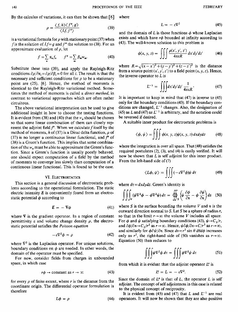
VII. CHARGED CONDUCTING PLATE Consider a square conducting plate 2a meters on a side

and lying on the z=O plane with center at the origin, as shown in Fig. 1. Let a(x, y ) represent the surface charge density on the plate, assumed to have zero thickness. The electrostatic potential at any point in space is

where R = ,/G - x’)’ + (y - y’)’ + z 2 . The boundary condition is 4 = V (constant) on the pIate. The integral equation for the problem is therefore

1x1 <a, ly( <a. The unknown to be determined is the charge density a ( x , y ) . A parameter of interest is the capacitance of the plate

which is continuous linear functional of a. A straightforward development of a subsection and point-

matching solution [lo] will first be given, and later it will be interpreted in terms of more general concepts. Consider the plate divided into N square subsections, as shown in Fig. 1 . Define functions

0 on all other As,,,

and let the charge density be represented by N

~ ( x , Y ) X E X . n = 1

Z

Fig. 1. A square conducting plate.

Substituting (60) into (57) and satisfying the resultant equation at the midpoint (x,,,, y,) of each As,,,, one obtains the set of equations

N V = 1 Imam m = 1 ,2 , . . . , N (61)

n= 1

where n ,

Note that 1, is the potential at the center of As,,, due to a uniform charge density of unit amplitude over As,,. A solution to the set (61) gives the G, in terms of which the charge density is approximated by (60). The corresponding capacitance of the plate, approximating (58), is

l N V n = 1 mn

C = - 1 a&,, = 1 l;‘Asn. (63)

This result can be interpreted as stating that the capacitance of an object is the sum of the capacitances of all its subsections plus the mutual capacitances between every pair of subsections.

To translate the above results into the language of linear spaces and the method of moments, let

Then f ) = g is equivalent to (57). A suitable inner product, satisfying (2) to (4), for which L is self adjoint, is

(f, s> = la d x l a dYf (x, Y ) g(x, Y ) . (67)

To apply the method of moments, use the function (59) as a subsectional basis, and define testing functions as

wrn = &X - - ym) (68)

which is the two-dimensional Dirac delta function. Now the elements of the [ I ] matrix (27) are those of (62) and the [SI matrix of (28) is

LvJ


The matrix equation (26) is, of course, identical to the set of equations (61). In terms of the inner product (67), the capacitance (58) can be written as

e=- (fl? 4) V2

(70)

since q5= V on the plate. Equation ( 7 9 is the conventional stationary formula for the capahtance of a conducting body [ 111.

For numerical results, the I,,,, of (62) must be evaluated. Let 2b = 2 a / f l denote the side length of each As,, The potential at the center of As, due to unit charge density over its own surface is

b b 1 IM = s- b dxJ- b dy 47c&J=

2b 2b = -In (1 + J?) = - (0.8814). (71) 7ZE 7LE

This derivation uses Dwight 200.01 and 731.2 [12]. The potential at the center of As,,, due to unit charge over As,, can be similarly evaluated, but the formula is complicated. For most purposes it is sufficiently accurate to treat the charge on h,, as if it were a point charge, and use

As, b2 I,, % ~ - - m # n. (72) 47~~Rmn XEJCXrn - X,)' + CVm - Y J 2

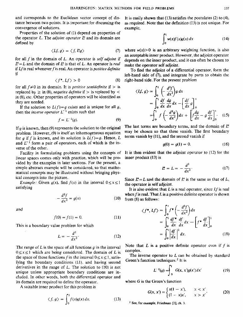
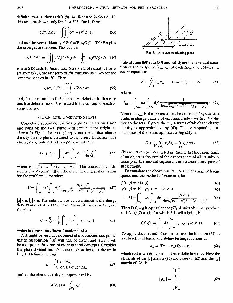
This approximation is 3.8 percent in error for adjacent subsections, and has less error for nonadjacent ones. Table I shows capacitance, calculated by (63) using the a's obtained from the solution of (61), for various numbers of subareas. The second column of Table I uses the approximation (72), the third column uses an exact evaluation of the I,,,,,. A good estimate of the true capacitance is 40 picofarads. Figure 2 shows a plot of the approximate charge density along the subareas nearest the center line of the plate, for the case N = 100 subareas. Note that 0 exhibits the well- known square root singularity at the edges of the plate.

TABLE I CAPACITANCE OF A SQUARE PLATE (PICOFARADS PER METER)

No. of subareas I C/2a approx. I,,,,, I C/2a exact I , I I

I 1 31.5 31.5 9 37.3 36.8

16 38.2 1 37.7 36 39.2 38.7

~

1 0 0 1 39.5

VIII. ELECTROMAGNETIC FIELDS The operator formulation of electromagnetic fields is

analogous to that of electrostatic fields, but considerably more complicated. For the time-harmonic case, do* varia- tion, the Maxwell equations are3

Only the case of electric sources is considered in this paper. The more general case of electric and magnetic sources is treated by the reaction concept [8], [9].

0 .I .2 .3 .4 .5 .6 .7 .8 .9 1.0 dtsiance along pbie

Fig. 2. Approximate charge density on subareas closest to the centerline of a square plate.

V x E = - j w p H V x H = j o s E + J (73)

where E is the electric field, H the magnetic field, and J the electric current density. Equations (73) can be combined into a single equation for E as

- V x (p-'V x E) - j w s E = J . - 1 (74)

This is of the form

L(E) = J (75)

where the operator L is evident from (74). For a specific case, let the permittivity and permeability be that of free space, that is, E = and p = p o . The domain of L must be restricted by suitable differentiability conditions on E, and boundary conditions on E must be given. To be specific, let these boundary conditions be the radiation condition, that is, the field must represent outward traveling waves at infinity.

The inverse operator is the well-known potential integral solution to (74), which is

E = L-'(J) = - j o A - VCD (76)

where

(79)

These equations can be combined into a single equation

E = L-'(J) = s s b ( r , r'). J(r')dr' (80)

where r is the dyadic Green's function. However, the derivation of (80) involves an interchange of integration and dif- ferentiation which restricts the domain of L- ' more than


necessary [13]. It is often better to consider (76) to (78) as the basic equations, with (80) as symbolic of them.

A suitable inner product for electromagnetic field problems is

(E, J ) = J j j E . J d t (81)

which is the quantity called reaction. Note that (81) satisfies postulates (2), (3), and (4). The concept of reciprocity is a statement of the self-adjointness of L-', that is,

( L - l J , , J 2 ) = (J1, L-'J2). (82)

The operator L is also self adjoint, since (82) can be written as

(El , LE2) = (LE, , E2) . (83)

Other properties of L can be determined as the need arises.

IX. WIRES OF ARBITRARY SHAPE An important engineering problem is the electromagnetic

behavior of thin wire objects. A general analysis of such objects according to the method of moments is presented in this section. The impressed field is considered arbitrary, and hence both the antenna and scatterer problems are in- cluded in the solution. The distinction between antennas and scatterers is primarily that of the location of the source. If the source is at the object it is viewed as an antenna; if the source is distant from the object it is viewed as a scatterer.

So that the development of the solution may be easily followed, it is given with few references to the general theory. Basically, it involves a) an approximation of the exact equation for conducting bodies by an approximate equation valid for thin wires, b) replacement of the derivatives by finite difference approximations, yielding an approximate operator, c) use of pulse functions for expansion functions, to give a step approximation to the current and charge, and d) the use of point-matching for testing.

A particularly descriptive exposition of the solution can be made in terms of network parameters. To effect a solution, the wire is considered as N short segments connected together. The end points of each segment define a pair of terminals in space. These Npairs of terminals can be thought of as forming an N port network, and the wire object is obtained by short-circuiting all ports of the network. One can determine the impedance matrix for the N port network by applying a current source to each port in turn, and calculat- ing the open circuit voltages at all ports. This procedure involves only current elements in empty space. The admittance matrix is the inverse of the impedance matrix. Once the admittance matrix is known, the port currents (current distribution on the wire) are found for any particular voltage excitation (applied field) by matrix multiplication.

An integral equation for the charge density as and current J , on a conducting body S in a known impressed field E' is obtained as follows. The scattered field E', produced by as and J, , is expressed in terms of retarded potential in-

\ n

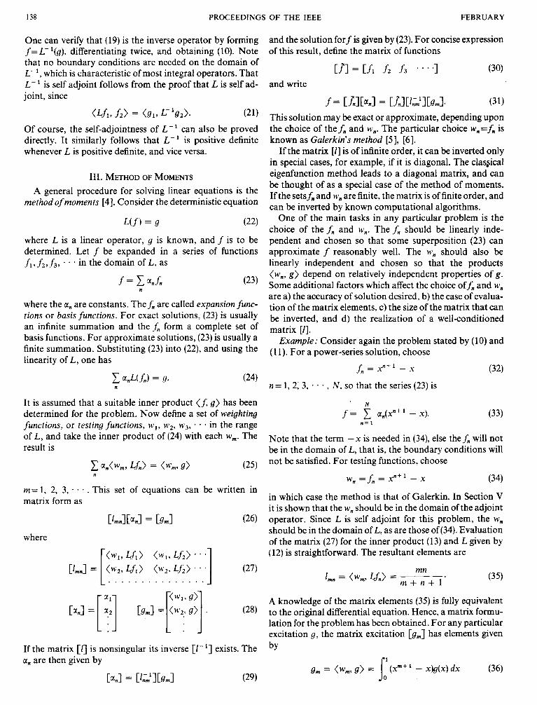
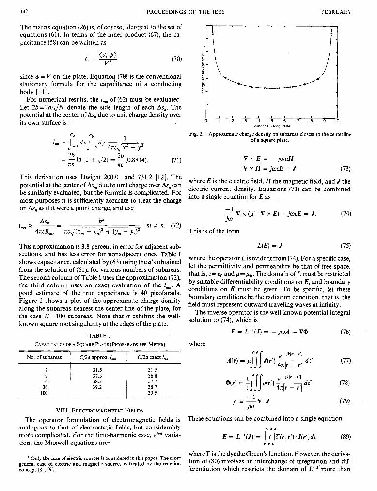
( a ) ( b ) Fig. 3. (a) A wire scatterer. (b) The wire axis divided into N segments.

tegrals, and the boundary condition n x (E'+ E') = 0 on S is applied. This is summarized by

Es = - j o A - v$ (84)

n x E , = - n x E' onS. (88)

Figure 3(a) represents an arbitrary thin-wire scatterer, for which the following approximations are made. a) The current is assumed to flow only in the direction of the wire axis. b) The current and charge densities are approximated by filaments of current Z and charge a on the wire axis. c) The boundary condition (88) is applied only to the axial component of E at the wire surface. To this approximation, (84) to (88) become

on S

e - j k R

dl axis

-1 d l a=-- jo dl

where I is the length variable along the wire axis, and R is measured from a source point on the axis to a field point on the wire surface.

A solution to the above equations is obtained as follows. Integrals are approximated by the sum of intergrals over N small segments, obtained by treating I and q as constant over each segment. Derivatives are approximated by finite differences over the same intervals used for integration. Figure 3(b) illustrates the division of the wire axis into N segments, and defines the notation. If a wire terminates, the boundary condition Z = O is taken into account by starting the first segment 1/2 interval in from the end of the wire. This is suggested in Fig. 3(b) by the extra 1/2 interval shown

1 4 4 PROCEEDINGS OF THE IEEE FEBRUARY

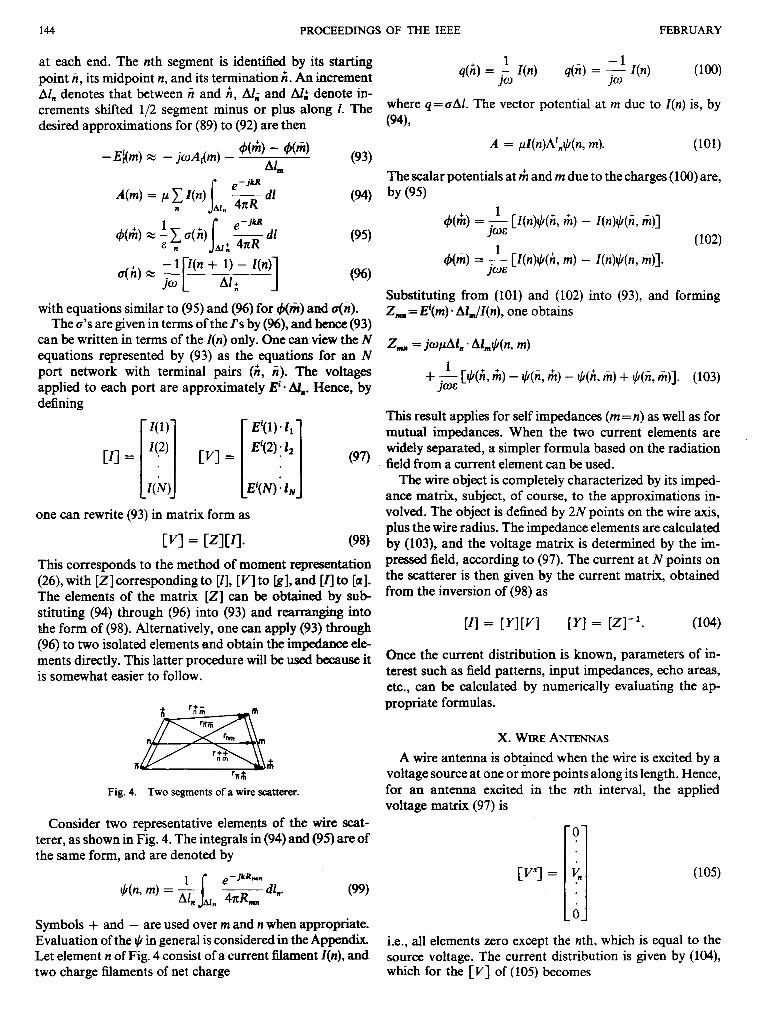
at each end. The nth segment is identified by its starting point ii , its midpoint n, and its termination ir . An increment Al, denotes that between n and ii, AI; and Al; denote in- crements shifted 1/2 segment minus or plus along 1. The desired approximations for (89) to (92) are then

a(h) x - - 1 Z(n + 1) - Z(n) 10 [ Aj: 1

(94)

with equations similar to (95) and (96) for &fi) and a(i). The 0's are given in terms of the l's by (%), and hence (93)

can be written in terms of the I(n) only. One can view the N equations represented by (93) as the equations for an N port network with terminal pairs (ir, i). The voltages applied to each port are approximately E' - A&. Hence, by defining

one can rewrite (93) in matrix form as

[VI = ~ZlC~I . (98) This corresponds to the method of moment representation (26), with [ Z ] corresponding to [ I ] , [VI to [g] , and [Il to [a]. The elements of the matrix [ Z ] can be obtained by sub stituting (94) through (96) into (93) and rearranging into the form of (98): Alternatively, one can apply (93) through (96) to two isolated elements and obtain the impedance elements directly. This latter procedure will be used because it is somewhat easier to follow.

Fig. 4. Two segments of a wire scatterer.

Consider two representative elements of the wire scatterer, as shown in Fig. 4. The integrals in (94) and (95) are of the same form, and are denoted by

Symbols + and - are used over m and n when appropriate. Evaluation of the + in general is considered in the Appendix. Let element n of Fig. 4 consist of a current filament I(n), and two charge filaments of net charge

where q=aAl. The vector potential at rn due to Z(n) is, by (941,

A = pZ(n)A*&(n, m). (101)

The scalar potentials at &I and i~ due to the charges (100) are, by (95)

4th) = - [Z(n)+(ii, rn) - I (n)$( i , rn)]. 1

JWE

Substituting from (101) and (102) into (93), and forming 2, = Ei(m) * AlJZ(n), one obtains

Z , = jo,uAl, * Alm+(n, m) 1

IWE + 7 [+(A, h) - $(it, h) - $(h, m) + $(i, m)]. (103)

This result applies for self impedances (rn = n) as well as for mutual impedances. When the two current elements are widely separated, a simpler formula based on the radiation field from a current element can be used.

The wire object is completely characterized by its impedance matrix, subject, of course, to the approximations involved. The object is defined by 2N points on the wire axis, plus the wire radius. The impedance elements are calculated by (103), and the voltage matrix is determined by the impressed field, according to (97). The current at N points on the scatterer is then given by the current matrix, obtained from the inversion of (98) as

[ I ] = [ Y ] [ V ] [ Y ] = [Z]? (104)

Once the current distribution is known, parameters of interest such as field patterns, input impedances, echo areas, etc., can be calculated by numerically evaluating the appropriate formulas.

X. WIRE ANTENNAS A wire antenna is obtained when the wire is excited by a

voltage source at one or more points along its length. Hence, for an antenna excited in the nth interval, the applied voltage matrix (97) is

i.e., all elements zero except the nth, which is equal to the source voltage. The current distribution is given by (104), which for the [VI of (105) becomes

1%7 HARRINGTON: MATRIX METHODS FOR FIELD PROBLEMS 145

Hence, the nth column of the admittance matrix is the current distribution for a unit voltage source applied to the nth interval. Inversion of the impedance matrix therefore gives simultaneously the current distributions when the antenna is excited in any arbitrary interval along its length. The diagonal elements Y, of the admittance matrix are the input admittances of the wire object fed in the nth interval, and the Y,, are the transfer admittances between a port in the mth interval and one in the nth interval.

The radiation pattern of a wire antenna is obtained by treating the antenna as an array of N current elements I(n)Al,. By standard formulas, the far-zone vector potential is given by

pe - i k r o A = - I(n)Al,e j k r , cos <,, (107)

471r0 n

where ro and r , are the radius vectors to the distant field point and to the source points, respectively, and <,, are the angles between ro and r,. The far-zone field components are

E , = - joA, E , = - joA, (108)

where 0 and 4 are the conventional spherical coordinate angles.

2

antenna

Y

Fig. 5. A wire antenna and distant dipole.

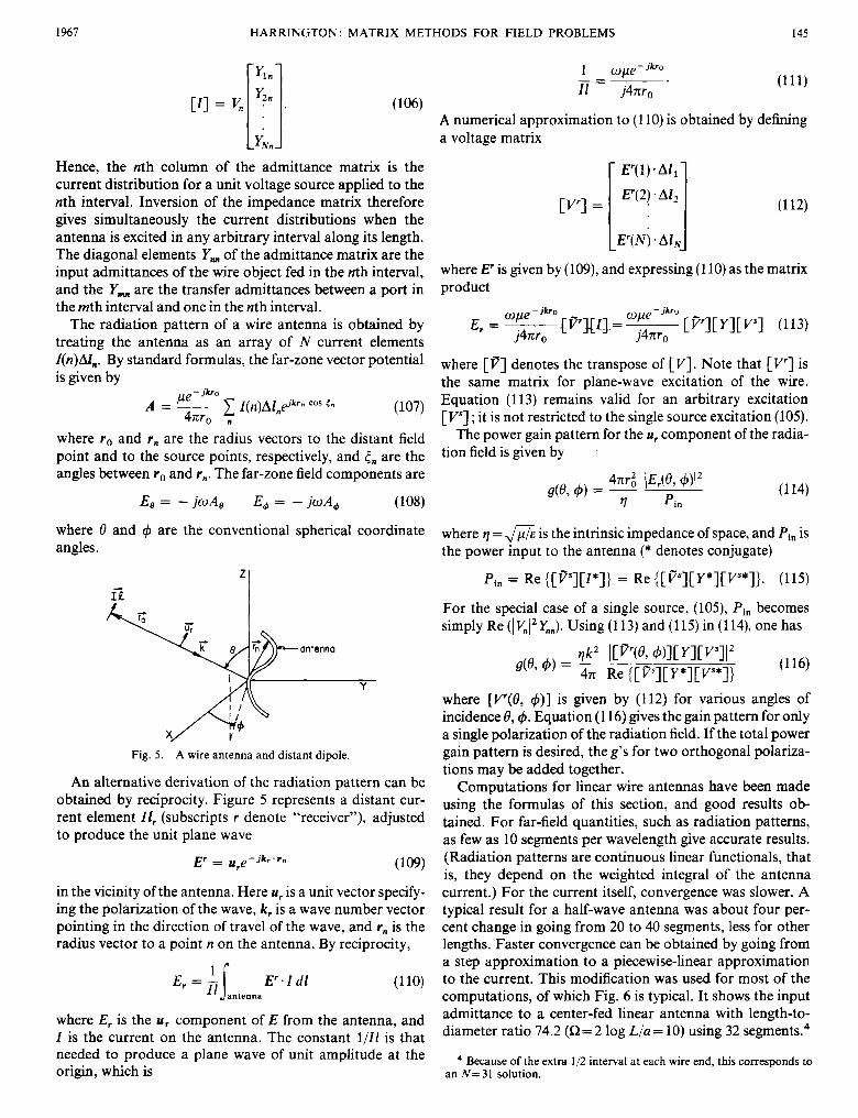
An alternative derivation of the radiation pattern can be obtained by reciprocity. Figure 5 represents a distant current element If, (subscripts r denote "receiver"), adjusted to produce the unit plane wave

,y = u , e - j k r ' r n

in the vicinity of the antenna. Here u, is a unit vector specify- ing the polarization of the wave, k, is a wave number vector pointing in the direction of travel of the wave, and rn is the radius vector to a point n on the antenna. By reciprocity,

(109)

E , = '1 E ' . I d l (1 10)

where E, is the u, component of E from the antenna, and I is the current on the antenna. The constant 1/11 is that needed to produce a plane wave of unit amplitude at the origin, which is

' 1 antenna

A numerical approximation to (1 10) is obtained by defining a voltage matrix

where E' is given by (109), and expressing (1 10) as the matrix product

where [PI denotes the transpose of [VI. Note that [Vr] is the same matrix for plane-wave excitation of the wire. Equation (1 13) remains valid for an arbitrary excitation [V"] ; it is not restricted to the single source excitation (105).

The power gain pattern for the u, component of the radiation field is given by

where q = f l~ is the intrinsic impedance of space, and Pin is the power input to the antenna (* denotes conjugate)

Pin = Re ([P"][Z*]> = Re {[P"][Y*][V'*]}. (115)

For the special case of a single source, (105), Pin becomes simply Re (I V , I 2 x,). Using (1 13) and (1 15) in (1 14), one has

s(4 4) = - 471 Re {[8"][Y*][Vs*]}

where [ V(0, 4)] is given by (1 12) for various angles of incidence e,& Equation (1 16) gives the gain pattern for only a single polarization of the radiation field. If the total power gain pattern is desired, the g's for two orthogonal polariza- tions may be added together.

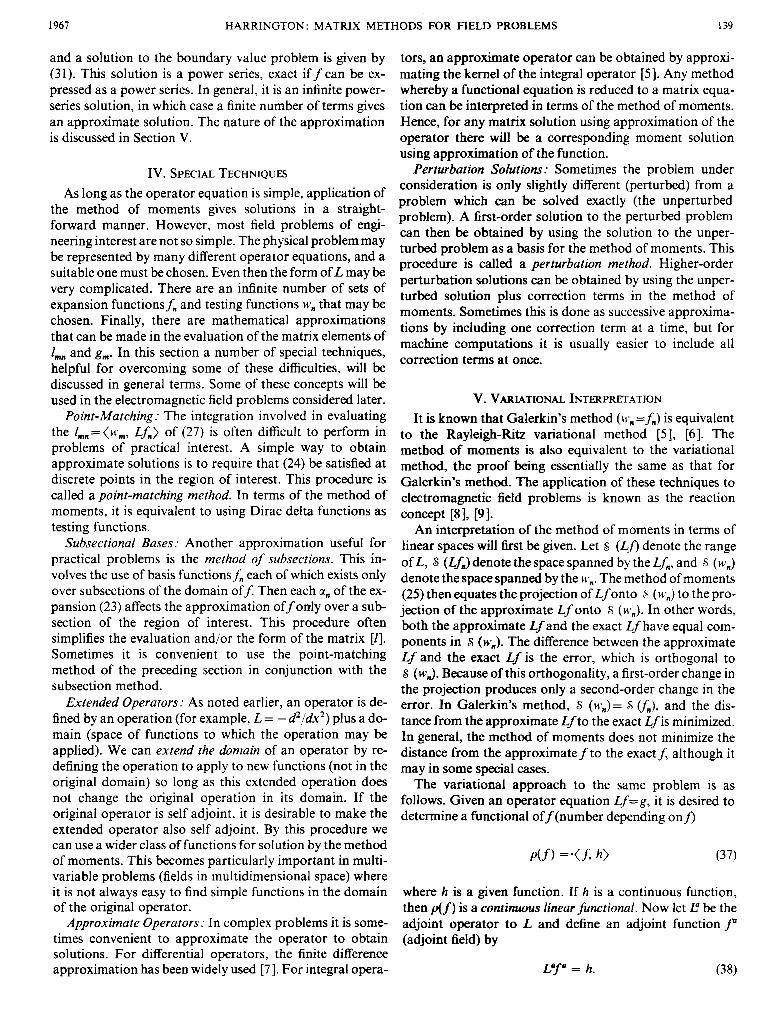
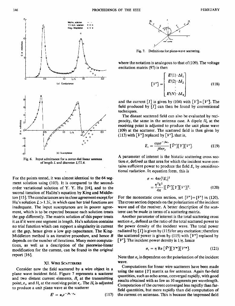
Computations for linear wire antennas have been made using the formulas of this section, and good results obtained. For far-field quantities, such as radiation patterns, as few as 10 segments per wavelength give accurate results. (Radiation patterns are continuous linear functionals, that is, they depend on the weighted integral of the antenna current.) For the current itself, convergence was slower. A typical result for a half-wave antenna was about four percent change in going from 20 to 40 segments, less for other lengths. Faster convergence can be obtained by going from a step approximation to a piecewise-linear approximation to the current. This modification was used for most of the computations, of which Fig. 6 is typical. It shows the input admittance to a center-fed linear antenna with length-to- diameter ratio 74.2 (SZ = 2 log L/a = 10) using 32 segment^.^

Because of the extra 1/2 interval at each wire end, this corresponds to an N=31 solution.


Fig. 7.

(01 Condudme

-6 (b) Suxeptance

Fig. 6. Input admittance for a center-fed hear antenna of length L and diameter Lp2.4.

For the points tested, it was almost identical to the 64 segment solution using (103). It is compared to the second- order variational solution of Y. Y. Hu [14], and to the second iteration of Hallen's equation by King and Middle- ton [ 151. The conductances are in close agreement except for Hu's solution L > 1.31, in which case her trial functions are inadequate. The input susceptances are in poorer agreement, which is to be expected because each solution treats the gap differently. The matrix solution of this paper treats it as if it were one segment in length. Hu's solution contains no trial function which can support a singularity in current at the gap, hence gives a low gap capacitance. The King- Middleton method is an iterative procedure, and hence B depends on the number of iterations. Many more computations, as well as a description of the piecewise-linear modification for the current, can be found in the original report [16].

XI. WIRE SCATTERERS

Consider now the field scattered by a wire object in a plane wave incident field. Figure 7 represents a scatterer and two distant current elements, ZZ, at the transmitting point, r,, and 11, at the receiving point r,. The Zl, is adjusted to produce a unit plane wave at the scatterer

/ Definitions for plane-wave scattering.

where the notation is analogous to that of (109). The voltage excitation matrix (97) is then

and the current [I] is given by (104) with [VI = [V']. The fkld produced by [Z] can then be found by conventional techniques.

The distant scattered field can also be evaluated by reciprocity, the same in the antenna case. A dipole Zl, at the receiving point is adjusted to produce the unit plane wave (109) at the scatterer. The scattered field is then given by (1 13) with [ V s ] replaced by [V'], that is,

A parameter of interest is the bistatic scattering cross section a, defined as that area for which the incident wave contains sufficient power to produce the field E, by omnidirec- tional radiation. In equation form, this is

a = 4nr,2(Er('

= - l[t'][Y][V']l'. q2k2 411

For the monostatic cross section, set [VI= [VI in (120). The cross section depends on the polarization of the incident wave and of the receiver. A better description of the scatterer can be made in terms of a scattering matrix.

Another parameter of interest is the total scattering cross section a,, defined as the ratio of the total scattered power to the power density of the incident wave. The total power radiated by [Z] is given by (1 15) for any excitation ; therefore the scattered power is given by (1 15) with [V'] replaced by [VI. The incident power density is 1/11, hence

a, = q Re [P'][Y*][V'*]. (121)

Note that a, is dependent on the polarization of the incident wave.

Computations for linear wire scatterers have been made using the same [ Y ] matrix as for antennas. Again far-field quantities, such as echo areas, converged rapidly, with good results obtained with as few as 10 segments per wavelength. Computation of the current converged less rapidly than far- field quantities, but more rapidly than did computation of

= , , e - j k . h (117) the current on antennas. This is because the impressed field

1967 HARRINGTON: MATRIX

-8 01 b 006

002

006

05 10 15 L/A

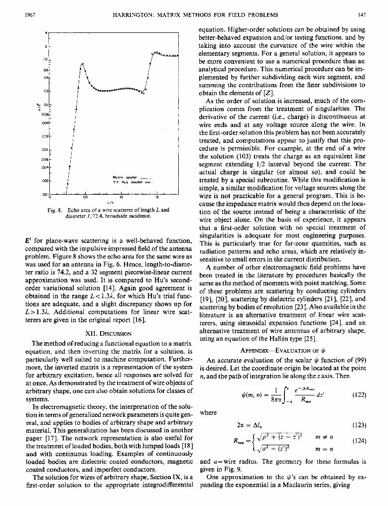
Fig. 8. Echo area of a wire scatterer of length L and diameter L/72.4, broadside incidence.

E' for plane-wave scattering is a well-behaved function, compared with the impulsive impressed field of the antenna problem. Figure 8 shows the echo area for the same wire as was used for an antenna in Fig. 6. Hence, length-to-diameter ratio is 74.2, and a 32 segment piecewise-linear current approximation was used. It is compared to Hu's second- order variational solution [14]. Again good agreement is obtained in the range L< 1.3& for which Hu's trial functions are adequate, and a slight discrepancy shows up for L> 1.31. Additional computations for linear wire scatterers are given in the original report [16].

XII. DISCUSSION The method of reducing a functional equation to a matrix

equation, and then inverting the matrix for a solution, is particularly well suited to machine computation. Further- more, the inverted matrix is a representation of the system for arbitrary excitation, hence all responses are solved for at once. As demonstrated by the treatment of wire objects of arbitrary shape, one can also obtain solutions for classes of systems.

In electromagnetic theory, the interpretation of the solution in terms of generalized network parameters is quite general, and applies to bodies of arbitrary shape and arbitrary material. This generalization has been discussed in another paper [ 171. The network representation is also useful for the treatment of loaded bodies, both with lumped loads [18] and with continuous loading. Examples of continuously loaded bodies are dielectric coated conductors, magnetic coated conductors, and imperfect conductors.

The solution for wires of arbitrary shape, Section IX, is a first-order solution to the appropriate integrodifferential

METHODS FOR FIELD PROBLEMS 147

equation. Higher-order solutions can be obtained by using better-behaved expansion and/or testing functions, and by taking into account the curvature of the wire within the elementary segments. For a general solution, it appears to be more convenient to use a numerical procedure than an analytical procedure. This numerical procedure can be im- plemented by further subdividing each wire segment, and summing the contributions from the finer subdivisions to obtain the elements of [Z].

As the order of solution is increased, much of the com- plication comes from the treatment of singularities. The derivative of the current (i.e., charge) is discontinuous at wire ends and at any voltage source along the wire. In the first-order solution t h s problem has not been accurately treated, and computations appear to justify that this procedure is permissible. For example, at the end of a wire the solution (103) treats the charge as an equivalent line segment extending 1/2 interval beyond the current. The actual charge is singular (or almost so), and could be treated by a special subroutine. Whle this modification is simple, a similar modification for voltage sources along the wire is not practicable for a general program. This is because the impedance matrix would then depend on the location of the source instead of being a characteristic of the wire object alone. On the basis of experience, it appears that a first-order solution with no special treatment of singularities is adequate for most engineering purposes. This is particularly true for far-zone quantities, such as radiation patterns and echo areas, which are relatively in- sensitive to small errors in the current distribution.

A number of other electromagnetic field problems have been treated in the literature by procedures basically the same as the method of moments with point matching. Some of these problems are scattering by conducting cylinders [19], [20], scattering by dielectric cylinders [21], [22], and scattering by bodies of revolution [23]. Also available in the literature is an alternative treatment of linear wire scatterers, using sinusoidal expansion functions [24], and an alternative treatment of wire antennas of arbitrary shape, using an equation of the HallCn type [25].

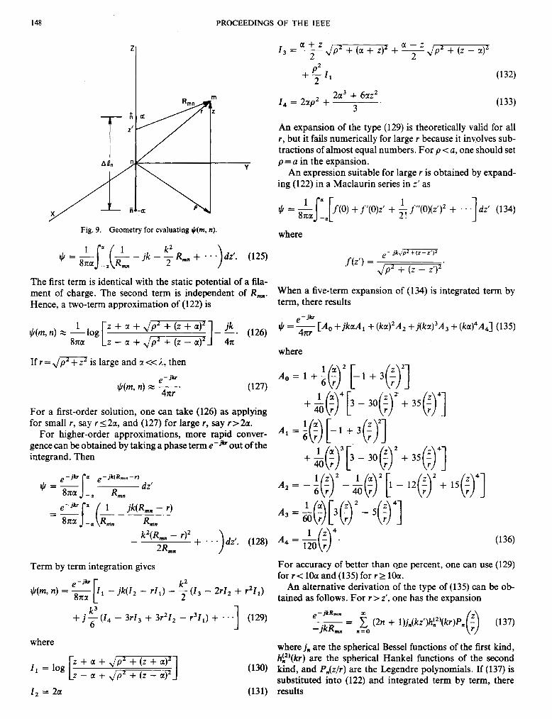
APPJWDM-EVALUATION OF t+h An accurate evaluation of the scalar t+h function of (99)

is desired. Let the coordinate origin be located at the point n, and the path of integration lie along the z axis. Then

1 F o-jkRmn

$(m, n ) = - ___ dz' ' J 8na - = R,,

where

and a = wire radius. The geometry for these formulas is given in Fig. 9.

One approximation to the $'s can be obtained by ex- panding the exponential in a Maclaurin series, giving

148 PROCEEDINGS OF THE IEEE

Y

Fig. 9. Geometry for evaluating $(m, n).

1 k2 8na --d R,, 2

$ = -r (-!- - j k - - R, + . . .

The first term is identical with the static potential of a filament of charge. The second term is independent of R,. Hence, a two-term approximation of (122) is

If r = is large and a <<A, then e-ib

$(m7 n) = T’ (127)

For a first-order solution, one can take (126) as applying for small r, say r 1 2 a , and (127) for large r, say r>2a.

For higher-order approximations, more rapid convergence can be obtained by taking a phase term e-Jb out of the integrand. Then

a + z 2

13=--J p2 + (a + z)2 + - J P 2 + ( z - a - z

2 P2 + - I , 2 (132)

2a3 + 6az2 3

I , = Zap’ + (133)

An expansion of the type (129) is theoretically valid for all r , but it fails numerically for large r because it involves sub- tractions of almost equal numbers. For p < a, one should set p = a in the expansion.

An expression suitable for large r is obtained by expand- ing (122) in a Maclaurin series in z’ as

+ . . -1 dz’ (134)

where

e - j k J p 2 + ( z - z ‘ ) 2

Jp2 + ( Z - 2’)‘ f (z’) =

When a five-term expansion of (1 34) is integrated term by term, there results

$ = - [Ao +jkaA, + (k~x)~A, + j ( k ~ r ) ~ A , + (ka),A,] (135) e - j b .

4m

where

A,, = 1 + L(F)2 6 r [-I + +->’I + -!-(!), 4 0 r [3 - 30(:)’ + 35(:),]

A , =

A , =

A , =

Term by term integration gives e-jb k2 8na !&7 4 = - - jk(12 - rI,) - - ( I 3 - 2r12 + ? I , )

2

where

I, = log [‘ + a + JP’ + (2 + a)‘] z - a + Jp’ + (z - a)’

- 35($

12(;)2

4 1

+ 15(:y]

For accuracy of better than oDe percent, one can use (129) for r < l0a and (135) for r 2 loa. An alternative derivation of the type of (135) can be ob-

tained as follows. For r > z’, one has the expansion e - j k R m n m -- - x (2n + l)j,(kz‘)hi2)(kr)P, -jkR, n = O

where j , are the spherical Bessel functions of the first kind, hi2)(kr) are the spherical Hankel functions of the second kind, and P,(z/r) are the Legendre polynomials. If (137) is substituted into (122) and integrated term by term, there results

PROCEEDINGS OF THE IEEE, VOL. 55, NO. 2, FEBRUARY, 1967

where

Equation (138) can be rearranged into the form of (135), although the recurrence formulas for hk2) and P , make computation directly from (138) almost as easy.

ACKNOWLEDGMENT The computer programming for the numerical results was

done by J. Mautz.

REFERENCES [ I ] B. Z. Vulikh, Introduction to Functional Analysis for Scientists and

Technologists, I. N. Sneddon, trans. Oxford: Pergamon, 1963. [2] B. Friedman, Principles and Techniques of Applied Mathematics. New

York: Wiley, 1956. [3] J. W. Dettman, Mathematical Methods in Physics and Engineering.

New York: McGraw-Hill, 1962. [4] L. Kantorovich and G. Akilov, Functional Analysis in Normed Spaces,

D. E. Brown, trans. Oxford: Pergamon, 1964, pp. 586-587. [5] L. Kantorovich and V. Krylov, Approximate Methods of Higher

Analysis, C. D. Benster, trans. New York: Wiley, 1964, ch. 4. [6] D. S. Jones, “A critique of the variational method in scattering an-

tennas,” IRE Trans. on Antennas and Propagation, vol. AP-4, pp. 297-301, July 1956.

[7] Forsythe and Wasov, Finite Dlfference Methods for Partial Differ- ential Equations. New York: Wiley, 1960.

[SI V. H. Rumsey, “The reaction concept in electromagnetic theory,” Phys. Rm., ser. 2, vol. 94, pp. 1483-1491, June 15, 1954.

[9] R. F. Hamngton, Time-Harmonic Electromagnetic Fields. New York: McGraw-Hill, 1961, pp. 34CL345.

[IO] D. K. Reitan and T. J. Higgins, “Accurate determination of the capacitance of a thin rectangular plate,” Trans. AIEE (Communica-

149

tion and Electronics), pt. I, vol. 75, pp. 761-766, 1956 (Jan. 1957 section).

[I I ] J. Van Bladel, Electromagnetic Fields. New York: McGraw-Hill, 1964, p. 96.

[I21 H. B. Dwight, Tables of Integrals and Other Mathematical Data. New York: Macmillan, 1947.

1131 J. Van Bladel, “Some remarks on Green’s dyadic for infinite space,” IRE Trans. on Antennas and Propagation, vol. AP-9, pp. 563-566, November 1961.

[I41 Yueh-Ying Hu, “Back-scattering cross section of a center-loaded cylindrical antenna,?’ IRE Trans. on Antennas and Propagation, vol. AP-6, pp. 14Q-148, January 1958.

[I51 R. W. P. King, The Theory of Linear Antennas. Cambridge, Mass.: Harvard University Press, 1956, p. 172.

[I61 R. F. Harrington et al.. “Matrix methods for solving field problems,” Rome Air Development Center, Griffiss AFB, N. Y., final rept. under Contract AF 30(602)-3724, March 1966.

[I71 R. F. Hamngton, “Generalized network parameters in field theory,” Proc. Symposium on Generalized Netnorks, MRIS series, vol. 16. Brooklyn, N. Y.: Polytechnic Press, 1966.

[I81 -, “Theory of loaded scatterers,” Proc. IEE (London). vol. 11 1, DD. 617-623. A ~ r i l 1964. K . K. Mei and i. G. Van Bladel, “Scattering by perfectlyconducting rectangular cylinders.” IEEE Trans. on Antennas and Propagation, vol. AP-11, pp. 185-192, March 1963. M. G. Andreasen, “Scattering from parallel metallic cylinders with arbitrary cross sections,” IEEE Trans. on Antennas and Propagation, vol. AP-12, pp. 746-754, November 1964. J. H. Richmond, “Scattering by a dielectric cylinder of arbitrary cross section shape,” IEEE Trans. on Antennas and Propagarion, vol. AP- 13, pp. 334-341, May 1965. -, “TE-wave scattering by a dielectric cylinder of arbitrary cross- section shape,” IEEE Trans. on Antennas and Propagation, vol.

M. G. Andreasen, “Scattering from bodies of revolution,” IEEE Trans. on Antennas and Propagation, voi. AP-13, pp. 303-310, March 1965. J. H. Richmond, “Digital computer solutions of the rigorous equations for scattering problems,” Proc. IEEE, vol. 53, pp. 796804, August 1965. K. K. Mei, “On the integral equations of thin wire antennas,” IEEE Trans. on Antennas and Propagation, vol. AP-13, pp. 374-378, May 1965.

AP-14, pp. 46@464, July 1966.

Digital Filter Design Techniques in the Frequency Domain

CHARLES M. RADER, MEMBER, IEEE, AND BERNARD GOLD

Manuscript received August 24,1965; final revision November 4,1966. The authors are with the Lincoln Laboratory, Massachusetts Institute

of Technology, Lexington, Mass. (Operated with support from the U. S. Air Force.)

SECTION I A . Introduction

D IGITAL FILTERING is the process of spectrum shaping using digital hardware as the basic building block. Thus the aims of digital filtering are the same

as those of continuous filtering, but the physical realization

matrix methods for field problems - oregon state...

Documents