matrix assisted laser desorptionllonisation time-of-flight
TRANSCRIPT
Matrix Assisted Laser Desorptionllonisation Time-of-Flight
Mass Spectroscopic Analysis of Synthetic Polymers
Marten Francis Snel
Presented for the degree of PhD
The University of Edinburgh cy-
1999

To Alison
Abstract
Matrix assisted laser desorption/ionisation time-of-flight mass spectrometry was used to mass analyse a range of synthetic polymers. Synthetic polymers with average molecular weights of up to 20000 Da were investigated. The polymers studied included polyglycols, polystyrene and poly(methyl methacrylate). Information on the repeat units, endgroups and average molecular weights was obtained.
A detailed study of novel copolymers was made, in which the end-group masses and the repeat unit masses of the polymers were determined. From this information combined with information of the polymer synthesis it was possible to propose detailed structures for the polymers studied.
An improved sample preparation technique was developed. This technique used an aerosol spray to deposit the matrix and analyte onto the sample holder. The new sample preparation technique made it possible to collect a large number of mass spectra with good reproducibility.
The stability of metal ion/polymer adducts was studied for poly(ethylene glycol) (PEG), poly(propylene glycol) (PPG) and poly(methyl methacrylate) (PMMA) adducts of lithium, sodium, potassium and rubidium, as well as the silver ion adduct of polystyrene. No post source decay (PSD) was seen for the lithium and sodium adducts of PEG, PPG and PMMA, however potassium and rubidium adducts of these polymers did undergo PSD. Rubidium adducts were seen to decay more readily than the potassium adducts.
Pulsed-field delayed ion extraction experiments were carried out. These experiments suggest that gas-phase reactions contribute comparatively little to the cation adduct formation of synthetic polymers. Further experiments showed that the ratio between salt and matrix in the sample did not affect the ionisation behaviour.
During the course of this work several improvements were made to the mass spectrometer used. The length of the time-of-flight mass analyser was increased and an in-line detector was fitted to the existing instrument. The addition of the second detector made it possible to operate the instrument in a linear mode. A mass gate was added to make it possible to avoid detector saturation by low-mass ions.

Acknowledgements Great thanks go to Robert Donovan whose enthusiastic encouragement and guidance have been a great help to me. I would also like to thank John Monaghan for his support and help over the past four years. The instrumental side of things would have been very much more daunting and less fun without the support of Robert Maier. Ian Mowat has been great for helping me to get started and for the many discussions.
I am also very grateful to Andy Cormack for writing me some extremely useful programs which saved me a great deal of time. I also would like to thank Annette and Mags for their friendly help.
The other 'mass spec' people, Alan, Brian, Angela Alison Michel, Mike and Pat all deserve a big thank you for the many chats (not all mass spec) and the occasional borrowed spanner.
Thanks to Mike, Paul and Sandy and all the rest of the coffee room crowd you all have been and always will be great friends to me.
A special thank you goes to Alison for her loving support throughout this work and beyond. My parents also have my deepest gratitude for all their support over the years;
I would also like to thank Franz Haaf for turning me onto chemistry.
Finally I would like to thank The University of Edinburgh and Procter and Gamble Ltd for financial support.
There are many more people that have been there for me and I am sorry that I haven't been able to name them all in person. Thanks.
Iv
Table of contents Declaration Abstract iii Acknowledgements iv Table of contents v List of figures viii List of tables xv List of abbreviations xvi
Chapter 1 - Introduction I 1.1 Introduction to MALDI mass spectrometry 1 1.2 Time-of-flight mass analysis 2
1.2.1 Instrumental strategies for enhancing the resolution of time- 6 of-flight mass analysers
1.3 lonisation and desorption in MALDI 7 1.3.1 Desorption mechanism 7 1.3.2 Ionisation mechanism 8
1.4 Introduction to polymer chemistry 12 1.5 Polymer mass determination 14 1.6 Polymer mass analysis by MALDI mass spectrometry 16
1.6.1 The range of polymers that have be analysed by MALDI 16 1.6.2 Matrices used in polymer MALDI 20 1.6.3 MALDI mass analysis of polydisperse polymers 22
1.6.3.1 Solutions to the polydisperse polymer analysis problem 22 1.6.4 Other polymer MALDI studies 23
1.7 References 24
Chapter 2 - Instrumentation :29 2.1 Introduction 29 2.2 The ion source 31 2.3 Time-of-flight mass analyser 32
2.3.1 Reflectron Design 33 2.4 Detectors and data analysis 36 2.5 The Mass Gate 38
2.5.1 Illustration of the effectiveness of the mass gate 41 2.6 Laser System 47 2.7 Pumping system 48 2.8 Conclusion 49 2.9 References 50
Chapter 3 - Sample preparation 51 3.1 Introduction 51 3.2 Choice of matrix and salt 52 3.3 Sample deposition 54
3.3.1 The droplet method 57 3.3.2 Electrospray sample deposition 59 3.3.3 The aerosol method 63
3.4 Conclusions 65 3.5 References 67
Chapter 4— Analysis of high-mass polymers 68 4.1 Introduction 68 4.2 Detection Systems 68 4.3 Sample Preparation 70 4.4 Results 72
4.4.1 Poly(ethylene glycol) 73 4.4.2 Polystyrene 75 4.4.3 Poly(rnethyl methacrylate) 77
4.5 Comparison of MALDI results with GPC results 78 4.5.1 Number averaged molecular weight 79 4.5.2 Weight averaged molecular weight 80 4.5.3 Polydispersity '81
4.6 Fragmentation of polymers 81 4.7 Conclusions 89 4.8 References 90
Chapter 5 - Metal ion detachment studies 91 5.1 Introduction 91 5.2 Experimental 92 5.3 Results and discussion 94
5.3.1 Qualitative survey of a range of polymer metal ion systems 95 5.3.2 Post acceleration 104 5.3.3 Altering the reflectron voltage 107 5.3.4 Experiments on the variation of the laser energy 113 5.3.5 Lower laser energy experiments 114
5.3.5.1 Results for PEG and L1CI 116 5.3.5.2 Results for PEG and NaCl 118 5.3.5.3 Results for PEG and KCI 121 5.3.5.4 Results for PEG and RbCl 125 5.3.5.5 Conclusions of the lower laser energy experiments 128
5.5.6 Higher laser energy experiments 129 5.5.7 Effect of fragmentation on the mass distribution of 136 polydisperse polymers
5.4 Conclusions 140 5.5 References 141
Vi
Chapter 6 - Delayed extraction experiments 142 6.1 Introduction 142 6.2 Experimental 144
6.2.1 Treatment of results 146 6.3 Results 147
6.3.1 Results obtained for delayed extraction experiments with 147 varying salt concentrations 6.3.2 Results obtained for other polymer salt systems 156 6.3.3 Initial ion velocities 160
6.4 Conclusions 160 6.5 References 162
Chapter 7— Copolymer analysis 163 7.1 Introduction to copolymer analysis 163 7.2 Synthesis of the copolymer samples 163 7.3 MALDI sample preparation and mass analysis 164 7.4 Results 165
7.4.1 Predicted products 165 7.4.2 Results for Samplel and Sample 2 168 7.4.3 Results for Sample 3 and Sample 4 170 7.4.4 Results for Sample 5 and Sample 6 176
7.5 Conclusions 180 7.6 References 181
Chapter 8 - Conclusions and further work 182 8.1 Introduction 182 8.2 Practical development of MALDI mass spectrometry for 183 synthetic polymers 8.3 Studies of the MALDI process 184 8.4 Results not included 184 8.5 Future work 185
Appendix I 187
Appendix II 199
List of figures Figure Title Page
1.1 Schematic representation of a linear time-of-flight mass 5 spectrometer.
1.2 The formation of polyethylene, as an example of chain 13 polymerisation.
1.3 The reaction to form nylon 6, 10, as an example of a typical 14 step polymerisation mechanism.
1.4 Typical matrix compounds employed in polymer mass 21 analysis by MALDI
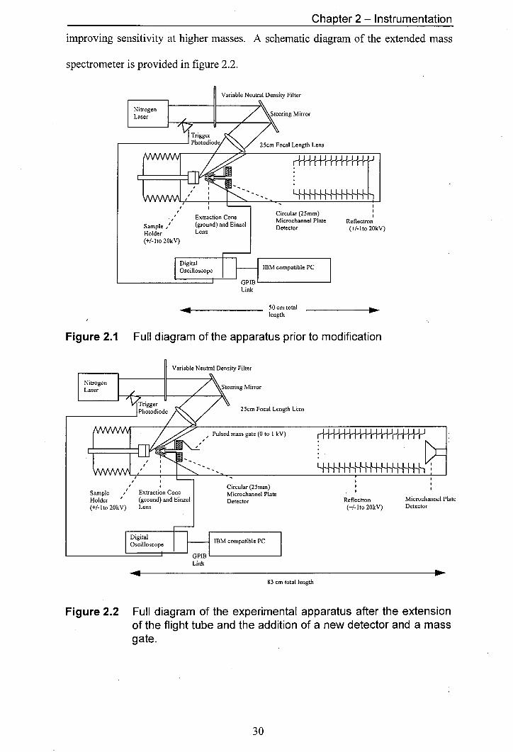
2.1 Full diagram of the apparatus prior to modification 30
2.2 Full diagram of the experimental apparatus after addition of 30 a new detector and a mass gate.
2.3 Diagram of the ion optics 31
2.4 Schematic diagram of the time-of-flight mass spectrometer, 34 prior to modification
2.5 Schematic diagram of the time-of-flight mass spectrometer 34 after the flight tube extension
2.6 Original reflectron design 35
2.7 Modified reflectron used after flight tube extension 35
2.8 Mounting for the reflectron detector 37
2.9 Voltage dividers for the reflectron detector 37
2.10 Voltage dividers for the linear detector 38
2.11 Diagram showing the mounting for the mass gate in front of 39 the reflectron detector.
Figure Title Page
2.12 The effect of the use of the mass gate on the time-of-flight 43 spectrum of PPG 1000. An extraction voltage of 12kV was used and the period of time for which the mass gate was left on was varied as shown ((a) to (c)). The mass gate was not used for the time-of-flight spectrum shown in (d).
2.13 The effect of the use of the mass gate on the time-of-flight 44 spectrum of PPG 1000. An extraction voltage of 16kV was used and the period of time for which the mass gate was left on was varied as shown ((a) to (d)). The mass gate was not used for the time-of-flight spectrum shown in (e).
2.14 The effect of the use of the mass gate on the time-of-flight 46 spectrum of PEG 2000 recorded in the reflectron mode. Spectrum (a) was recorded with the mass gate switched off. - When spectrum (b) was recorded the mass gate was left on for 2 js at 100 V.
3.1 Electrospray sample preparation apparatus 60
3.2 Example of polystyrene mass spectrum produced using the 61 electrospray sample prepration method. Dithranol was used as the matrix and AgCF3CO2 as the salt.
3.3 Reproducibility of signal intensity obtained using the 62 electrospray method. The variation in normalised peak areas of the 1 2-mer peak of polystyrene from a series of spectra collected from the same sample holder is shown.
3.4 Reproducibility of signal intensity obtained using the aerosol 65 method. The variation in normalised peak areas of the 42-mer peak of poly(ethylene glycol) from a series of spectra collected from the same sample holder is shown.
4.1 Change in ion velocity with ion mass
4.2 MALDI mass spectrum of PEG (av. mol. wt. 8500), HABA 72 was used as the matrix and LiCl as the cation donor
4.3 Expansion of the polymer distribution shown in figure 4.2 73
4.4 Mass spectrum of PEG (av. mol. wt. 11000 Da), the matrix 74 used was HABA and the salt used was LiCI
ix
Figure Title
4.5 MALDI mass spectrum of polystyrene (av. mol. wt. 11000 Da), trans-retinoic acid was used as the matrix and Ag NO3 as the salt.
4.6 MALDI mass spectrum of polystyrene (av. mol. wt. 20000 Da), trans-retinoic acid was used as the matrix and Ag NO3 as the salt.
4.7 MALDI mass spectrum for PMMA, the matrix used was HABA and the added salt was LiCI
4.8 Expansion of high-mass region shown in figure 4.7
4.9 Mass spectrum of polystyrene 12860 with an unusual sloping feature (mlz = 4000— 10000). The matrix used was dithranol and the salt used was AgCF3CO2
4.10 Mass spectrum for PEG exhibiting a sloping background
4.11 Expansion of the sloping part of figure 4.10
4.12 Suggested fragmentation pathways for poly(ethylene glycol)
4.13 Plot of Observed endgroup mass vs observed oligomer mass.
4.14 Schematic illustration of the effect of the mass gate on ions located in different parts of the mass spectrometer.
4.15 Endgroup mass vs oligomer mass used to determine average endgroup masses
5.1 Operation of the mass spectrometer in linear mode
5.2 Operation of the mass spectrometer in reflectron mode with reflectron voltage above extraction voltage.
5.3 MALDI Mass Spectra of PEG with different salts added to provide cations for adduct formation. In the top traces only neutrals are observed whilst in the bottom traces, both neutrals and ions are observed.
Page
75
76
77
78
82
83
84
85
86
87
88
93
94
96
x
Figure Title Page
5.4 MALDI Mass Spectra of PMMA with different salts added to 97 provide cations for adduct formation. In the top traces only neutrals are observed whilst in the bottom traces, both neutrals and ions are observed.
5.5 MALDI Mass Spectra of PPG with different salts added to 98 provide cations for adduct formation. In the top traces only neutrals are observed whilst in the bottom traces, both neutrals and ions are observed.
5.6 MALDI TOF Mass spectra of PEG with a mixture of salts. In 102 the top traces only neutrals are observed whilst in the bottom traces, both neutrals and ions are observed.
5.7 Time-of-flight mass spectra of rubidiUm PEG adducts 106 recorded at 108 .iJ laser energy. The traces in a) were recorded with post acceleration whereas the traces in b) were recorded without post acceleration.
5.8 Time-of-flight spectra of lithium PEG adducts recorded at 108 varying reflectron voltages.
5.9 The shift in flight time vs voltage applied to the reflectron for 109 selected peaks.
5.10 Time-of-flight spectra of rubidium PEG adducts recorded at 111 varying reflectron voltages.
5.11 Enlargement of figure 5.10 showing the presence of neutral 112 peaks in all traces indicated by the doffed lines.
5.12 Time-of-flight Spectra of PEG with LiCI with the Reflectron 115 off, recorded at laser energy varying between 69 tJ and 108 J.
5.13 Time-of-flight Spectra of PEG with LiCI with the Reflectron 115 on, recorded at laser energy varying between 69 iJ and 108 [tJ.
5.14 Time-of-flight Spectra of PEG with NaCl with the Reflectron 119 off, recorded at laser energy varying between 69 pJ and 108 pJ.
Xi
Figure Title Page
5.15 Time-of-flight Sectra of PEG with NaCl with the Reflectron 119 on, recorded at laser energy varying between 69 pJ and 108 j.tJ.
5.16 Time-of-flight Spectra of PEG with KCJ with the Reflectron 121 off, recorded at laser energies varying between 69 pJ and 108 jiJ.
5.17 Time-of-flight Spectra of PEG with KCI with the Reflectron 122 on, recorded at laser energy varying between 69 j.iJ and 108 iJ.
5.18 A comparison between the Signal intensity of neutrals vs 124 laser energy and the signal intensity of the combined neutrals and ions vs laser energy for three PEG oligomer potassium adducts.
5.19 Time-of-flight Spectra of PEG with RbCl with the Reflectron 126 off, recorded at laser energy varying between 69 pJ and 108 J.
5.20 Time-of-flight Spectra of PEG with RbCl with the Reflectron 126 on, recorded at laser energy varying between 69 tJ and 108 [1J.
5.21 A comparison between the Signal intensity of neutrals vs 127 laser energy and the signal intensity of the combined neutrals and ions vs laser energy for three PEG oligomer rubidium adducts.
5.22 Time-of-flight spectra of PEG with LiCI with the reflectron off 131 recorded at laser energies between 76 pJ and 158 pJ.
5.23 Time-of-flight spectra of PEG with LiCl with the reflectron on 132 recorded at laser energies between 76 pJ and 158 pJ.
5.24 Time-of-flight spectra of PEG with RbCl with the reflectron 134 off recorded at laser energies between 76 p.J and 158 pJ.
5.25 Time-of-flight spectra of PEG with RbCl with the reflectron 135 on recorded at laser energies between 76 pJ and 158 pJ.
xii
Figure Title Page
5.26 Mass spectra of a mixture of potassiated PEG 1000 and 139 PEG 3400 recorded using three different detection systems.
The mass spectrum was recorded on the linear detector with the reflectron switched on; only neutrals are observed.
The mass spectrum was recorded on the linear detector with the reflectron switched off; both ions and neutrals are observed. c) The mass spectrum was recorded on the reflectron detector with the reflectron switched on; only reflected ions are observed.
6.1 Schematic illustration of the instrument layout for delayed 145 extraction operation
6.2 Example of the trigger sequence for the high voltage 146 extraction pulse. The synchronous output from the N2 laser triggers the pulse generator, which in turn triggers the high voltage switch.
6.3 Effect of delayed ion extraction on the MALDI mass spectra 148 of polystyrene. In the bottom trace no delay between the laser shot and ion extraction was used for the other traces, a delay of between 100 ns and 600 ns was used, as shown. The matrix used was dithranol and the salt used was AgCF3CO2. The matrix to salt ratio was I to 5.
6.4 The variation in normalised peak areas for a range of 150 different polystyrene oligomer silver adducts with delay time. The matrix used was dithranol and the salt used was AgCF3CO2. The mole ratio of Dithranol to AgCF3CO2 used was 10:1.
6.5 The variation in normalised peak areas for a range of 151 different polystyrene oligomer silver adducts with delay time. The matrix used was dithranol and the salt used was AgCF3CO2. The mole ratio of Dithranol to AgCF3CO2 used was 2:1.
6.6 The variation in normalised peak areas for a range of 151 different polystyrene oligomer silver adducts with delay time. The matrix used was dithranol and the salt used was AgCF3CO2. The mole ratio of Dithranol to AgCF3CO2 used was 1:1.
Figure Title Page
6.7 The variation in normalised peak areas for a range of 152 different polystyrene oligomer silver adducts with delay time. The matrix used was dithranol and the salt used was AgCF3CO2. The mole ratio of Dithranol to AgCF3CO2 used was 1:2.5.
6.8 The variation in normalised peak areas for a range of 152 different polystyrene oligomer silver adducts with delay time. The matrix used was dithranol and the salt used was AgCF3CO2. The mole ratio of Dithranol to AgCF3CO2 used was 1:5.
6.9 Averaged peak area responses of a range of silver 155 polystyrene oligomer adducts to delay time for a range of different AgCF3CO2 to dithranol ratios
6.10 Variation of normalised peak areas for different PMMA 157 oligomer lithium adducts with delay time. The matrix used was dithranol with LiCI at a mole ratio of 1:1. Delay time range for this experiment was 0 ns to 400 ns.
6.11 Variation of normalised peak areas for different PMMA 157 oligomer lithium adducts with delay time. The matrix used was dithranol with LiCI at a mole ratio of 1:1. Delay time range for this experiment was 0 ns to 1000 ns.
6.12 Variation of normalised peak areas for different PEG 158 oligomer sodium adducts with delay time. The matrix used was dithranol and the salt used was NaCl at a mole ratio of 1:1. Delay time range for this experiment was 0 ns to 400 ns.
6.13 Variation of normalised peak areas for different PEG 158 oligomer sodium adducts with delay time. The matrix used was dithranol with NaCl at a mole ratio of 1:1. Delay time range for this experiment was 0 ns to 1000 ns.
6.14 Illustration of the shift in time-of-flight seen under delayed 159 extraction conditions owing to the initial velocity of ions. The peaks shown are silver adducts of the 10-mer of polystyrene.
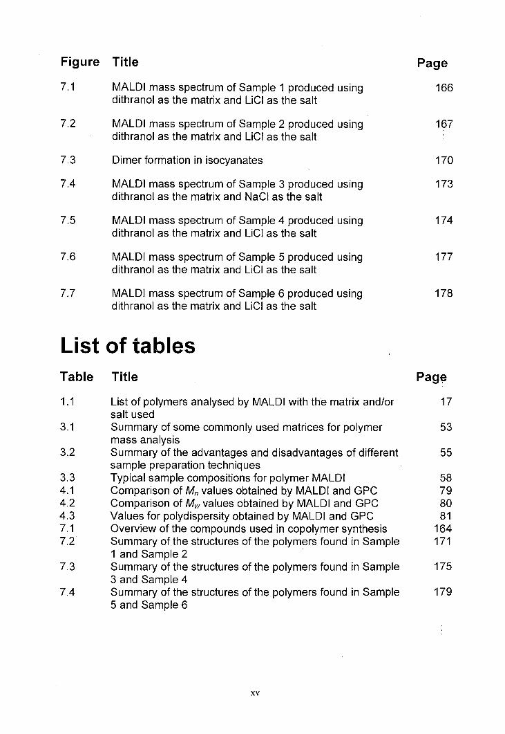
Figure Title Page
7.1 MALDI mass spectrum of Sample 1 produced using 166 dithranol as the matrix and LiCl as the salt
7.2 MALDI mass spectrum of Sample 2 produced using 167 dithranol as the matrix and LiCl as the salt
7.3 Dimer formation in isocyanates 170
7.4 MALDI mass spectrum of Sample 3 produced using 173 dithranol as the matrix and NaCl as the salt
7.5 MALDI mass spectrum of Sample 4 produced using 174 dithranol as the matrix and LiCl as the salt
7.6 MALDI mass spectrum of Sample 5 produced using 177 dithranol as the matrix and LiCl as the salt
7.7 MALDI mass spectrum of Sample 6 produced using 178 dithranol as the matrix and LiCl as the salt
List of tables Table Title Page
1.1 List of polymers analysed by MALDI with the matrix and/or 17 salt used
3.1 Summary of some commonly used matrices for polymer 53 mass analysis
3.2 Summary of the advantages and disadvantages of different 55 sample preparation techniques
3.3 Typical 'sample compositions for polymer MALDI 58 4.1 Comparison of M values obtained by MALDI and GPC 79 4.2 Comparison of M values obtained by MALDI and GPC 80 4.3 Values for potydispersity obtained by MALDI and GPC 81 7.1 Overview of the compounds used in copolymer synthesis 164 7.2 Summary of the structures of the polymers found in Sample 171
1 and Sample 2 7.3 Summary of the structures of the polymers found in Sample 175
3 and Sample 4 7.4 Summary of the structures of the polymers found in Sample 179
5 and Sample 6
xv
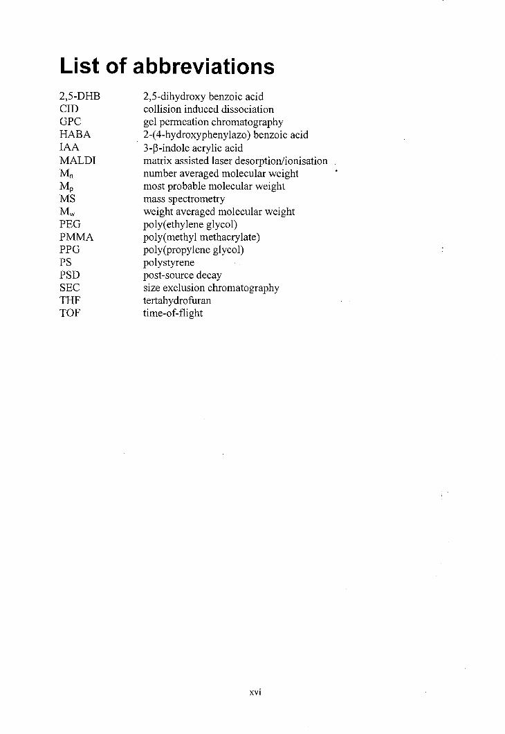
List of abbreviations 2,5-DHB 2,5-dihydroxy benzoic acid CID collision induced dissociation GPC gel permeation chromatography HABA 2-(4-hydroxyphenylazo) benzoic acid IAA 3-13-indole acrylic acid MALDI matrix assisted laser desorption/ionisation Mn number averaged molecular weight M most probable molecular weight MS mass spectrometry
weight averaged molecular weight PEG poly(ethylene glycol) PMMA poly(methyl methacrylate) PPG poly(propylene glycol) PS polystyrene PSD post-source decay SEC size exclusion chromatography THF tertahydrofuran TOF time-of-flight
xvi

List of poster presentations 22 nd Meeting of the British Mass Spectrometry Society (BMSS), University of Wales Swansea, Swansea, September 1996
Autumn Meeting and Pre-Doctoral Symposium of The Royal Society of Chemistry, University of Aberdeen, Aberdeen September 1997
1998 National Congress and Young Researchers' Meeting of The Royal Society of Chemistry, University of Durham, Durham April 1998
xvii
Chapter 1 - Introduction
Chapter 1 - Introduction
1.1 Introduction to MALDI mass spectrometry
The last sixteen years have seen a revolution in the mass analysis of high
molecular mass species [1]. The effective mass-spectrometric analysis of very large
molecules with minimal fragmentation has been made possible by the
introduction/development of two soft ionisation techniques namely electrospray
ionisation (ESI) [2] and matrix assisted laser desorption/ionisation (MALDI) [3,4].
The work presented in this dissertation focuses on MALDI.
MALDI, as the name suggests, was developed from laser ablation techniques.
Unlike conventional laser desorption, the molecules to be analysed are dispersed
through a matrix during sample preparation. The matrix is usually solid, consisting
of small organic molecules, although various liquid matrix systems have been
reported [4,5]. In order to produce molecular ions, with MALDI, only one pulsed
laser focused on the sample is required. The most commonly used lasers are the
nitrogen laser [6] and frequency tripled [7] and quadrupled [8] Nd:YAG lasers, both
emitting ns pulses of UV radiation. However JR MALDI has also been reported
[9,10]. Positive and negative analyte species can both be produced by MALDI. In
positive ion experiments quasi-molecular analyte ions are the most common analyte
species detected. These usually take the form of proton or cation complexes usually
Chapter 1 - Introduction
referred to as adducts [11]. Negative ion experiments tend to yield ions formed by
the loss of a proton [12].
Since its advent, MALDI has been used to study a number of different types
of large molecules, including proteins, peptides [11], oligosaccharides [13], nucleic
acids [14] and synthetic polymers [15]. The focus of this work is on the synthetic
polymer mass analysis by MALDI. A detailed discussion of polymer MALDI
experiments follows in section 1.5.
1.2 Time-of-flight mass analysis
The most commonly used mass analyser in conjunction with MALDI is the
time-of-flight (TOF) mass analyser. Some experiments have been reported where
other mass analysers such as sector instruments [16] and Fourier-transform ion
cyclotron resonance mass spectrometers (FTICR-MS) [17] have been used. Time-of-
flight mass analysers have several features that make them ideal for use with MALDI
sources. Possibly the most important of these is that, in principle, TOF analysers
have no upper mass limit. Another desirable attribute of a TOF analyser is the
detection of all ions with every laser shot.
Michael Guilhaus's recently published tutorial on the principles of and
instrumentation in time-of-flight mass spectrometry gives a good background to this
technique [18]. The basic principle behind TOF mass separation is that ions moving
in the same direction with roughly the same kinetic energy will have a distribution of
2
Chapter 1 - Introduction
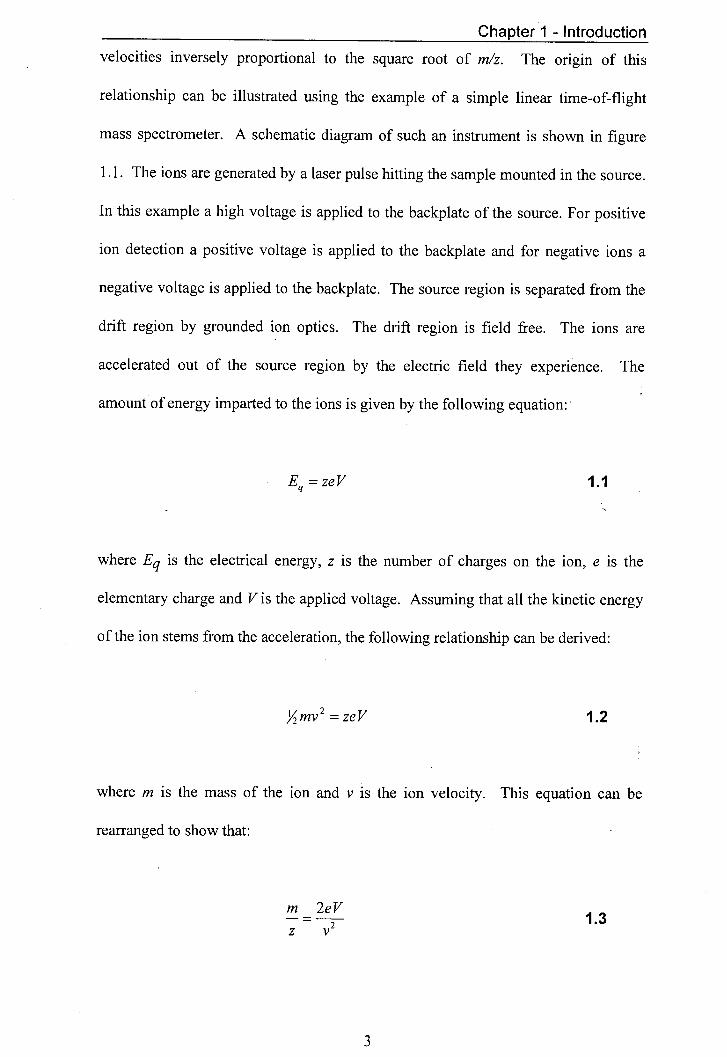
velocities inversely proportional to the square root of m/z. The origin of this
relationship can be illustrated using the example of a simple linear time-of-flight
mass spectrometer. A schematic diagram of such an instrument is shown in figure
1.1. The ions are generated by a laser pulse hitting the sample mounted in the source.
In this example a high voltage is applied to the backplate of the source. For positive
ion detection a positive voltage is applied to the backplate and for negative ions a
negative voltage is applied to the backplate. The source region is separated from the
drift region by grounded ion optics. The drift region is field free. The ions are
accelerated out of the source region by the electric field they experience. The
amount of energy imparted to the ions is given by the following equation:
Eq =zeV
1.1
where Eq is the electrical energy, z is the number of charges on the ion, e is the
elementary charge and V is the applied voltage. Assuming that all the kinetic energy
of the ion stems from the acceleration, the following relationship can be derived:
Y, MV , = zeV
1.2
where m is the mass of the ion and v is the ion velocity. This equation can be
rearranged to show that:
m2eV 1.3
z
3
Charter 1 - Introduction
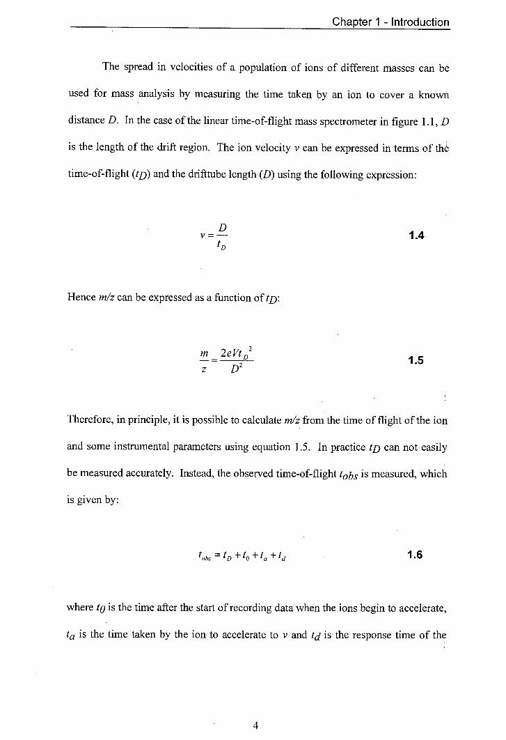
The spread in velocities of a population of ions of different masses can be
used for mass analysis by measuring the time taken by an ion to cover a known
distance D. In the case of the linear time-of-flight mass spectrometer in figure 1. 1, D
is the length of the drift region. The ion velocity v can be expressed in terms of the
time-of-flight (tD) and the drifttube length (D) using the following expression:
D V 1.4 ti,
Hence m/z can be expressed as a function of tD:
rn2eVt D 2 1.5
z D
Therefore, in principle, it is possible to calculate m/z from the time of flight of the ion
and some instrumental parameters using equation 1.5. In practice tD can not easily
be measured accurately. Instead, the observed time-of-flight tobs is measured, which
is given by:
tubs = tD + to + ta + td 1.6
where to is the time after the start of recording data when the ions begin to accelerate,
ta is the time taken by the ion to accelerate to v and td is the response time of the
I
Drift Region
0 v2 M.) m2
Source D
Detector
Chapter 1 - Introduction
detection system. In practice it is therefore easiest to convert time-of-flight
information into m/z using the following equation:
M2 -= AtollS + BtObS. + C z
1.7
where A, B and C are instrument constants that can be determined by calibration of
the mass spectrometer with ions of known mass.
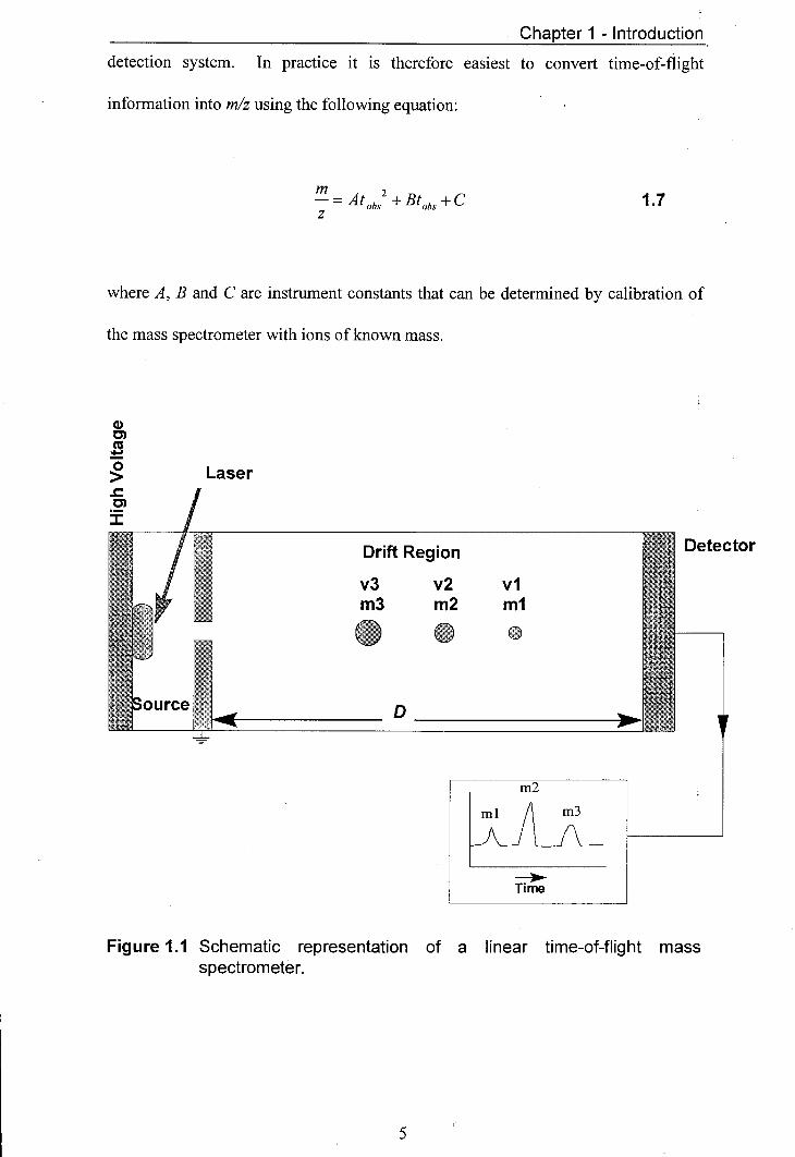
Laser
Figure 1.1 Schematic representation of a linear time-of-flight mass spectrometer.
5
Chapter 1 - Introduction
1.2.1 Instrumental strategies for enhancing the resolution of time-of-flight
mass analysers
The resolution of linear time-of-flight instruments used with MALDI sources
is limited by the kinetic energy spread of ions produced by MALDI [19]. Two
techniques are widely used for the correction of the kinetic energy spread. One is the
use of an ion mirror, usually referred to as a reflectron and the other technique is
delayed extraction or time-lag focusing.
Reflectrons are probably the most widely used method for improving the
resolution of time-of-flight mass spectrometers. Reflectrons are essentially ion
mirrors which reverse the direction of travel of the ion [20]. A detailed description
of the coaxial reflectron used in this work is given in Chapter 2. The small difference
in ion velocity between ions of the same mass is compensated for by the reflectron
as ions with higher kinetic energy penetrate more deeply and therefore take longer to
be reflected, similarly ions with lower kinetic energy penetrate the reflecting field
less deeply and hence are reflected more quickly.
Delayed extraction is based on the idea of time-lag focusing, which was
originally proposed by Wiley and McLaren [21]. Delayed extraction has been shown
to be an effective method for improving the resolution of MALDI TOF
systems. [22,23,24,25] In delayed extraction experiments, there is a time delay
between the laser hitting the sample and the acceleration of the ions out of the source
region of the mass spectrometer. The ions are allowed to spread out in space before
Chapter 1 - Introduction
the acceleration potential is applied. As the ions have reached different positions in
the source at the time of acceleration, they will receive differing amounts of kinetic
energy from acceleration. With the right delay time, it is largely possible to
compensate for the kinetic energy spread of ions and hence bring about an
improvement in resolution.
1.3 lonisation and desorption in MALDI
Although MALDI is a technique that is widely used in commercial
laboratories, the MALDI process(es) is/are as yet not completely understood.
However, a great deal of work has gone into furthering the understanding of matrix
assisted laser desorption and matrix assisted laser ionisation. The next two sections
give an overview of this area. For simplicity's sake desorption and ionisation are
discussed separately.
1.3.1 Desorption mechanism
Matrix assisted laser desorption (MALD) is believed to be brought about by
rapid local heating of the matrix leading to vaporisation of the matrix [26]. As the
hot matrix material expands away from the sample surface it takes with it analyte
species. Although the matrix is heated rapidly little fragmentation is seen of the
analyte molecules. This has been accounted for by modelling studies showing that
the matrix to analyte molecule energy transfer-is limited [27].
7
Chapter 1 - Introduction
1.3.2 lonisation mechanism
Cation-molecule complexes are the most commonly detected species in
positive ion MALDI. The ion formation mechanisms are still largely unknown. Ions
may exist as pre-formed species in the solid state or may. be formed by ion-molecule
reactions initiated by the laser shot or, most probably, ions are formed by a
combination of these two processes [28]. The matrix is believed to play an important
part in the ionisation processes in MALDI [29].
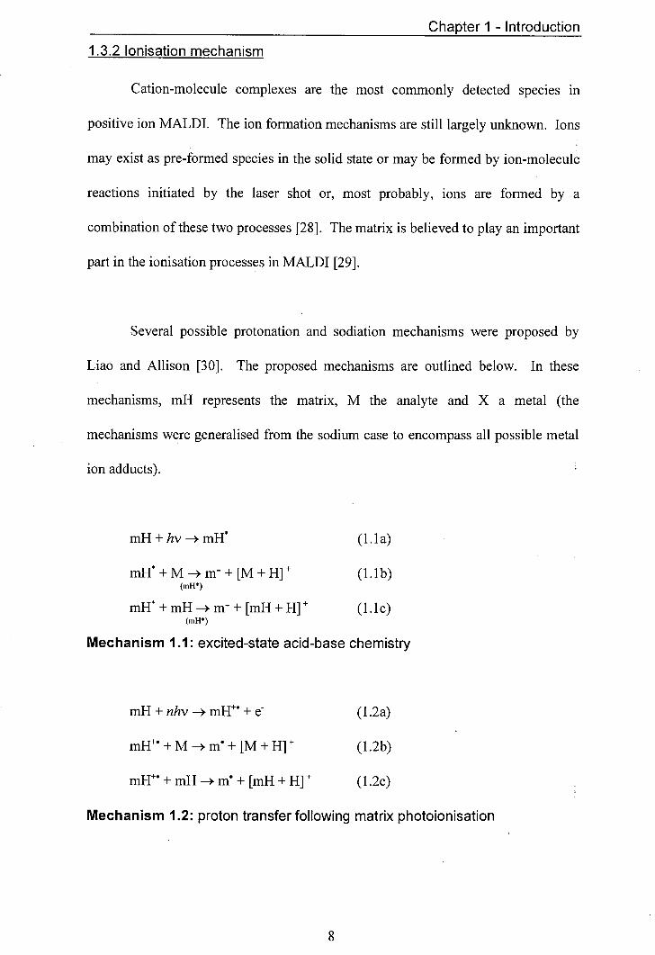
Several possible protonation and sodiation mechanisms were proposed by
Liao and Allison [30]. The proposed mechanisms are outlined below. In these
mechanisms, mH represents the matrix, M the analyte and X a metal (the
mechanisms were generalised from the sodium case to encompass all possible metal
ion adducts).
mH+hv+mH* (1.la)
mH* +M>m+[M+H]+ (1.lb) (mH*)
mH* +mH_m+ [mH +H]+ (l.lc) (mH*)
Mechanism 1.1: excited-state acid-base chemistry
mH+nhv—*mH+e (1.2a)
mH+M-+m+[M+H] (1.2b)
mH+mH—*m+ [mH +H] (1.2c)
Mechanism 1.2: proton transfer following matrix photoionisation
Chapter 1 - Introduction
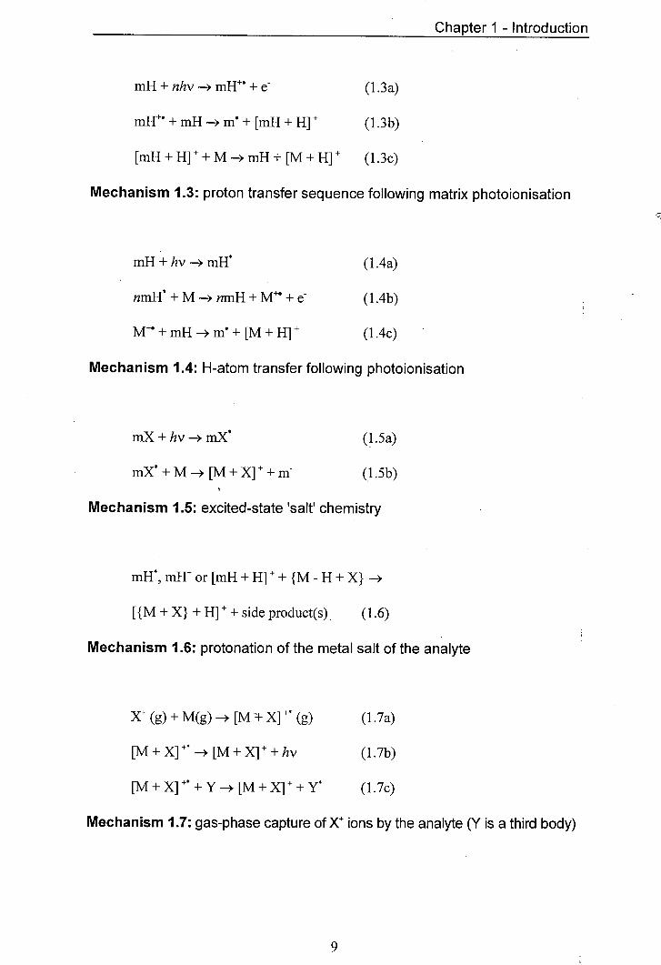
mH+nhv-*mH+e (1.3a)
mH'* + mH - m + [mH + H] + (1.3b)
[mH +H]+M->mH+[M+H] (1.3c)
Mechanism 1.3: proton transfer sequence following matrix photolonisation
mH+hv-+mH (1.4a)
nmH* + M nmH + M + e (1.4b)
M + mH - m + [M + H] + (1.4c)
Mechanism 1.4: H-atom transfer following photolonisation
mX+hv-*mX' (1.5a)
mX*+M>[M+X]++m (1.5b)
Mechanism 1.5: excited-state 'salt' chemistry
mH*,,mH+or [mH +H]++{MH+X}-
[{M + X} + H] + + side product(s) . (1.6)
Mechanism 1.6: protonation of the metal salt of the analyte
X(g)+M(g)-* [M±X]+* (g) (1.7a)
[M+X]-*[M+X]+hv (1.7b)
[M+X]+*+Y>[M+X]++Y* (1.7c)
Mechanism 1.7: gas-phase capture of X ions by the analyte (Y is a third body)
Chapter 1 - Introduction
Evidence of gas phase reactions such as the ones described by mechanism 1.7
has been provided by delayed extraction experiments and by layered sample
preparation experiments [31,32,33]. Two delayed extraction studies have been
reported, one on small peptides and the other on synthetic polymers. Both
experiments showed that the analyte cation adduct signal intensity in MALDI mass
spectra increased if the extraction of the ions was delayed in time with respect to the
laser shot. Wang et al. carried out an experiment, where gas-phase Na ions were
introduced separately by laser ablation from a Nal surface perpendicular to the
MALDI sample holder. Mass spectra obtained when Na-ions were introduced prior
to the MALDI process showed a large increase in the signal intensity of sodium
adduct peaks of the analyte, suggesting gas-phase adduct formation. In the layer
experiments performed by Hoberg et al. a sandwich of two salt layers containing a
matrix analyte layer was prepared. The analyte was poly(methyl methacrylate)
(PMMA) and the matrix used was 1 ,8,9-trihydroxyanthracene (dithranol). Two
different salts, LiC1 and RbC1, were used for the top and the bottom salt layer with
both combinations being used. The interesting outcome of this experiment was that
only the cation present in the bottom salt layer formed adducts with PMMA. This
observation was rationalised as evidence for gas-phase cation adduction. The
assumption was made that metal ions move away from the surface more quickly than
the larger PMMA molecules and hence the metal ions produced from the top layer
have a far smaller chance to interact with the PMMA than the bottom layer ions. The
rapid separation of metal ions from PMMA neutrals in the high field gradient in the
MALDI source region would mean that ion molecule reaction would have to occur
near the surface in the gas plume.
10
Chapter 1 - Introduction
Evidence for an ionisation process analogous to mechanism 1.1 was reported
by Knochenmuss et al. [34]. This work suggests that the reactions 1.1 b and 1.1 c
only occur when at least two mH* species are present. The evidence for this
mechanism is that MALDI mass spectra can be obtained from samples with low
matrix concentrations in which no matrix signal is seen, the so called matrix
suppression effect. Matrix suppression Is thought to 'occur when the matrix
concentration is so low that when two photoexcited matrix molecules are nearest
neighbours in the solid they are always in close proximity to an analyte molecule. If
reaction 1. lb is strongly favoured over reaction 1. ic, little or no cationised matrix
species will be formed as the proton available would be used to form an analyte
adduct [34]. It can be seen from mechanism 1.1 that when no positive matrix species
are produced negative matrix ions, m, should be produced. Knochenmuss and co-
workers did observe a strong m signal in negative ion mass spectra obtained from
samples that showed matrix suppression in the positive ion mode. The same group
illustrated the requirement for two photoexcited matrix molecules to bring about
successful ionisation by diluting 2,5-dihydroxybenzoic acid (DHB) with CsI. It was
noted that at a mole ratio of CsI to DHB higher than 1:2, the DHB signal became
very weak which was interpreted as being due to the low likelihood of two
photoexcited DHB molecules being nearest neighbours.
In this section a number of ionisation mechanisms have been described. It is
not yet possible to say with certainty which mechanism(s) play(s) the most important
role in the ionisation mechanism in MALDI.
Chapter 1 - Introduction
1.4 Introduction to polymer chemistry
A good introduction to polymer chemistry can be found in most university
chemistry textbooks [35,36]. The word polymer is derived from the Greek words
'poly' meaning many and 'meros' meaning part. A polymer is a macromolecule that
is made up of a large number of smaller components known as monomers. The term,
polymer, covers a wide range of very different compounds. Polymers can be split
into two main categories; these are the biopolymers and the synthetic polymers.
Biopolymers include proteins, peptides, polysaccharides and nucleic acids.
Polythene, polystyrene, silicones and dendrimers are all examples of synthetic
polymers. This introduction will focus on synthetic polymers.
The first synthetic polymers to gain commercial importance were the
phenol-formaldehydes. They were discovered in the early 1890s by G. T. Morgan.
However, it was not until 1910 when Leo Bakeland founded the General Bakelite
Company that these compounds were used commercially. Despite the fact that
synthetic polymers were being manufactured the concept of macromolecules was
only introduced in 1920 by Hermann Staudinger. The macromolecular hypothesis
finally became established through the work of Wallace Carothers who set out in
1929 to synthesise polymers of definite structure using conventional organic
reactions. His work successfully demonstrated the relationship between structure and
properties for a number of polymers. He also invented polymers of great commercial
importance such as the nylons.
12
Chapter 1 - Introduction
Synthetic polymers consist of long linear or branched chains of monomers
forming one molecule. Simple linear polymers may be written as X-(A)-Y, where n
is an integer, A is the monomer or repeat unit and X and Y are endgroups. All
man-made polymeric materials consist of molecules with a range of different values
of n; moreover it is very difficult to isolate molecules with one discrete n value. The
abundance of molecules with a particular n value in a given polymer follows a
statistical distribution, which is affected by the reaction conditions used during the
synthesis of the polymer.
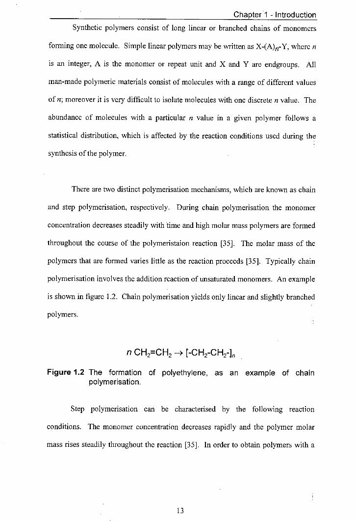
There are two distinct polymerisation mechanisms, which are known as chain
and step polymerisation, respectively. During chain polymerisation the monomer
concentration decreases steadily with time and high molar mass polymers are formed
throughout the course of the polymeristaion reaction [35]. The molar mass of the
polymers that are formed varies little as the reaction proceeds [35]. Typically chain
polymerisation involves the addition reaction of unsaturated monomers. An example
is shown in figure 1.2. Chain polymerisation yields only linear and slightly branched
polymers.
n CH2=CH2 - [-CH2-CH2-]
Figure 1.2 The formation of polyethylene, as an example of chain polymerisation.
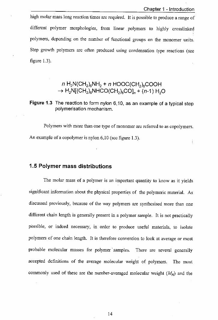
Step polymerisation can be characterised by the following reaction
conditions. The monomer concentration decreases rapidly and the polymer molar
mass rises steadily throughout the reaction [35]. In order to obtain polymers with a
13
Charter I - Introduction
high molar mass long reaction times are required. It is possible to produce a range of
different polymer morphologies, from linear polymers to highly crosslinked
polymers, depending on the number of functional groups on the monomer units.
Step growth polymers are often produced using condensation type reactions (see
figure 1.3).
n H2N(CH2)6NH2 + n HOOC(CH2)8COOH -> H2N[(CH2)6NHCO(CH2)8CO] + (n-i) H20
Figure 1.3 The reaction to form nylon 6,10, as an example of a typical step polymerisation mechanism.
Polymers with more than one type of monomer are referred to as copolymers.
An example of a copolymer is nylon 6,10 (see figure 1.3).
1.5 Polymer mass distributions
The molar mass of a polymer is an important quantity to know as it yields
significant information about the physical properties of the polymeric material. As
discussed previously, because of the way polymers are synthesised more than one
different chain length is generally present in a polymer sample. It is not practically
possible, or indeed necessary, in order to produce useful materials, to isolate
polymers of one chain length. It is therefore convention to look at average or most
probable molecular masses for polymer samples. There are several generally
accepted definitions of the average molecular weight of polymers. The most
commonly used of these are the number-averaged molecular weight (Mn) and the
14
Chapter 1 - Introduction
weight-averaged molecular weight (Mw) [35]. M is given by the following
equation:
M
1.8 Y Ni
where M1 is the molar mass of the molecular species i and Ni is the number of
molecules of i in the sample. The weight-averaged molar mass on the other hand is
given by:
M" Ni=
NM 1.9
M gives greater weighting to the lower molecular mass polymers in a polymer
sample, whereas Mw gives greater emphasis to the higher molecular mass part of a
polymer sample. The ratio of Mw to M is known as the polydispersity and is often
used as an indication of the spread of masses within a polymer sample. When
polymer samples have a very narrow spread of masses M/M1 these polymer
mass distribution are referred to as monodisperse. Similarly, if M,/M> 1, the
polymer sample has a wider spread of masses and is said to be polydisperse.
LI
15
Chapter 1 - Introduction
1.6 Polymer mass analysis by MALDI mass spectrometry
Traditional means of determining polymer mass information include size
exclusion chromatography (SEC), light scattering and viscometry [35]. These
techniques can yield accurate information on the average molecular weight and
polydispersity of polymers. They are however limited in that they do not provide
structural information on polymers. SEC also requires calibration using well defined
molecular weight standards, which means that molecular weights obtained using this
technique are relative to the standard [37].
MALDI is one of the most promising techniques for synthetic polymer
analysis. MALDI does not only give information on the average molecular weight of
polymers but can also provide end-group masses and repeat unit information. A
range of suitable matrix compounds for use in synthetic polymer analysis has been
identified. The number of different synthetic polymers that can be analysed by
MALDI is continuously increasing. Problem areas in the MALDI analysis of
polymers, such as the analysis of highly polydisperse polymers and the analysis of
hydrocarbon polymers have recently been addressed. Several reviews of synthetic
polymer MALDI have been published, which provide a good introduction to this area
of research [38,39].
1.6.1 The range of polymers be analysed by MALDI
A wide range of polymers can be analysed using MALDI MS. The capacity
of MALDI to yield detailed structural information, such as repeat unit mass and
ILO
Chapter 1 - Introduction
endgroup mass, has meant that it is becoming an increasingly widely used tool for
the mass analysis of low molecular weight polymers in commercial laboratories [40].
The most commonly used synthetic polymers in MALDI experiments are
poly(ethylene glycol) (PEG) and poly(propylene glycol) (PPG), polystyrene (PS) and
poly (methyl methacrylate) (PMMA). These particular polymers are used as model
systems. Samples whose average molar masses and polydispersity are well
characterised by means of other techniques are readily available, as these compounds
are often used to calibrate gel permeation chromatography systems [41]. They also
lend themselves particularly well to MALDI analysis [15]. Some of the studies in
which PMMA, PEG, PPG and PS have been used will be discussed in sections 1.6.3
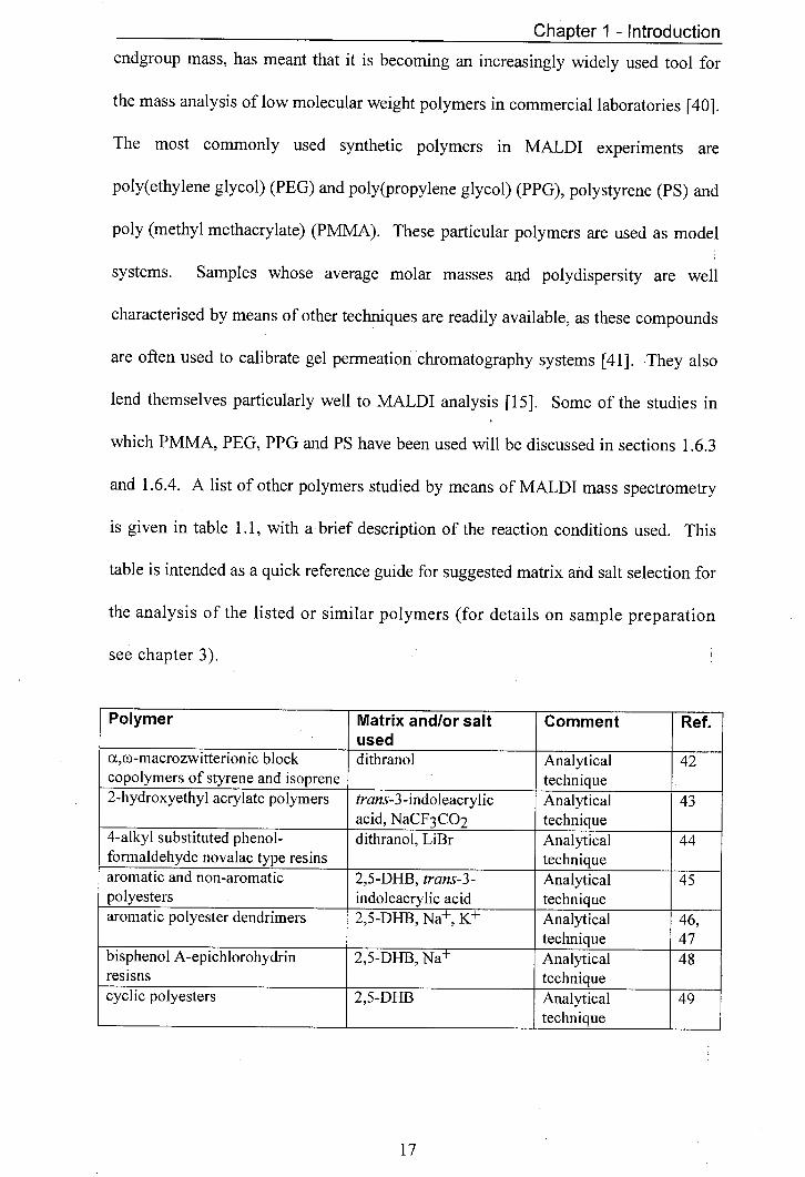
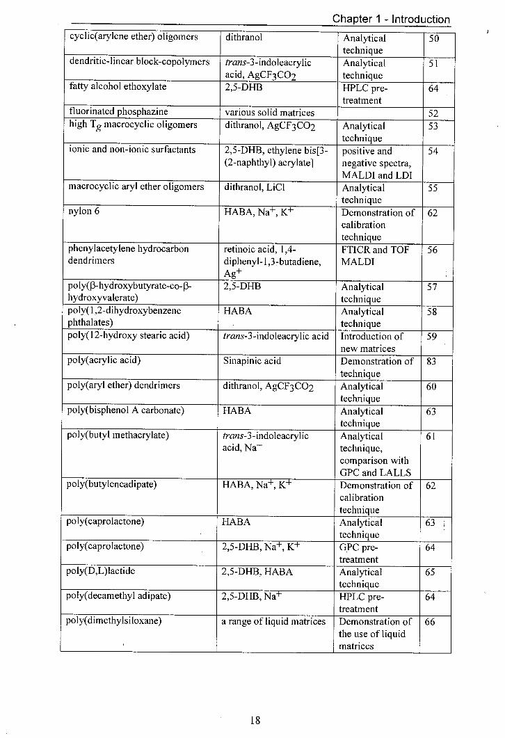
and 1.6.4. A list of other polymers studied by means of MALDI mass spectrometry
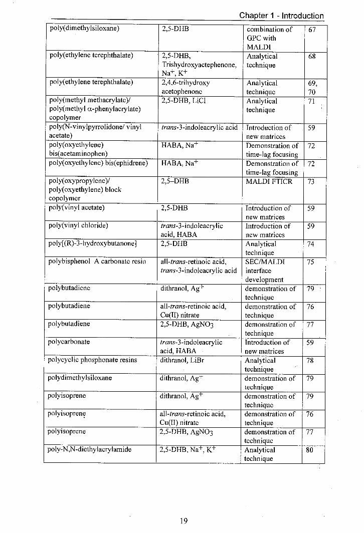
is given in table 1.1, with a brief description of the reaction conditions used. This
table is intended as a quick reference guide for suggested matrix and salt selection for
the analysis of the listed or similar polymers (for details on sample preparation
see chapter 3).
Polymer Matrix and/or salt Comment Ref. used
a,w-rnacrozwifterionic block dithranol Analytical 42 copolymers of styrene and isoprene technique 2-hydroxyethyl acrylate polymers trans-3-indoleacrylic Analytical 43
acid, NaCF3 CO2 technique 4-alkyl substituted phenol- dithranol, LiBr Analytical 44 formaldehyde novalac type resins technique aromatic and non-aromatic 2,5-DHB, trans-3- Analytical 45 polyesters indoleacrylic acid technique aromatic polyester dendrimers 2,5-DEB, Na+, K+ Analytical 46,
__________ technique 47 bisphenol A-epichlorohydrin 2,5-DHB, Na Analytical 48 resisns technique cyclic polyesters 2,5-DHB Analytical 49
technique
17
Chapter 1 - Introduction
cyc!ic(arylene ether) oligomers dithranol Analytical 50 technique
dendritic- linear block-copolymers trans-3-indoleacrylic Analytical 51 acid, AgCF3CO2 technique
fatty alcohol ethoxylate 2,5-DHB HPLC pre- 64 treatment
fluorinated phosphazine various solid matrices 52 high Tg macrocyclic oligomers dithranol, AgCF3CO2 Analytical 53
technique ionic and non-ionic surfactants 2,5-DHB, ethylene bis[3- positive and 54
(2-naphthyl) acrylate] negative spectra, MALDI and LDI
macrocyclic aryl ether oligomers dithranol, LICI Analytical 55 _____________ technique
nylon 6 HABA, Na+, K+ Demonstration of 62 calibration technique
phenylacetylene hydrocarbon retinoic acid, 1,4- FTICR and TOF 56 dendrimers diphenyl- 1,3 -butadiene, MALDI
Ag 0 ly(13-hydroxybutyrate-co- 13- 2,5-DHB Analytical 57
hydroxyvalerate) technique poly( 1 ,2-d ihydroxybenzene HABA Analytical 58 phthalates) technique poly( 1 2-hydroxy stearic acid) trans-3 - indoleacrylic acid Introduction of 59
new matrices poly(acrylic acid) Sinapinic acid Demonstration of 83
technique po!y(aryl ether) dendrimers dithranol, AgCF3CO2 Analytical 60
technique poly(bisphenol A carbonate) HABA Analytical 63
technique poly(butyl methacrylate) trans-3 -indoleacrylic Analytical 61
acid, Na+ technique, comparison with GPC and LALLS
poly(butyleneadipate) HABA, Na+, K+ Demonstration of 62 calibration technique
poly(caprolactone) HABA Analytical 63 technique
poly(caprolactone) 2,5-DHB, Nat, K GPC pre- 64 treatment
poly(D,L)lactide 2,5-DHB, HABA Analytical 65 technique
poly(decamethyl adipate) 2,5-DHB, Na HPLC pre- 64 treatment
poly(dimethylsiloxane) a range of liquid matrices Demonstration of 66 the use of liquid matrices
18
Chapter 1 - Introduction
poly(dimethylsiloxane) 2,5-DUB combination of 67 GPC with MALDI
poly(ethylene terephthalate) 2,5-DUB, Analytical 68 Trishydroxyactephenone, technique Na+, K+
poly(ethylene terephthalate) 2,4,6-trihydroxy Analytical 69, acetophenone technique 70
poly(methyl methacrylate)/ 2,5-DUB, L1CI Analytical 71 poly(methyl (x-phenylacrylate) technique copolymer poly(N-vinylpyrrolidone/ vinyl trans-3-indoleacrylic acid Introduction of 59 acetate) new matrices poly(oxyethylene) HABA, Na+ Demonstration of 72 bis(acetarninophen) time-lag focusing poly(oxyethylene) bis(ephidrene) HABA, Na Demonstration of 72
time-lag focusing poly(oxypropylene)/ 2,5—DUB MALDI FTICR 73 poly(oxyethylene) block copolymer poly(vinyl acetate) 2,5-DUB Introduction of 59
new matrices poly(vinyl chloride) trans-3-indoleacrylic Introduction of 59
acid, HABA new matrices poly[(R)-3 -hydroxybutanone] 2,5-DHB Analytical 74
technique polybisphenol A carbonate resin all-trans-retinoic acid, SEC/MALDI 75
trans-3-indoleacrylic acid interface ___________ development
polybutadiene dithranol, Ag+ demonstration of 79 technique
polybutadiene all-trans-retinoic acid, demonstration of 76 Cu(II) nitrate technique
polybutadiene 2,5-DHB, AgNO3 demonstration of 77 technique
polycarbonate trans-3-indoleacrylic Introduction of 59 acid, HABA new matrices
polycyclic phosphonate resins dithranol, LiBr Analytical 78 ___________ technique
polydimethylsiloxane dithranol, Ag+ demonstration of 79 __________ technique
polyisoprene dithranol, Ag+ demonstration of 79 technique
polyisoprene all-trans-retinoic acid, demonstration of 76 Cu(II) nitrate technique
polyisoprene 2,5-DHB, AgNO3 demonstration of 77 __________ technique
poly-N,N-diethylacrylamide 2,5-DHB, Nat, K Analytical 80 technique
19
Chapter 1 - Introduction
polyorganometallic ferrocene Dithranol, quinizarin, Analytical 81 derivative HABA, 9-nitroanthracene technique polysilabutane 2,5-DHB Analytical 82
technique polystyrene sulphonic acid Sinapinic acid Demonstration of 83
technique polystyrene/ poly(a- trans-3-indoleacrylic Analytical 84 methyistyrene) block copolymer acid, silver technique
acetylacetonate polystyrene-ol igothiophene- Analytical 85 polystyrene triblock copolymer technique polyvinyl pyrrolidone 2,5-DHB MALDI FTICR 86 triazine based polyamines 2,5-DHB in formic acid Analytical 87
technique triblock 2,5-DHB, Li Critical point LC 64 ethyleneoxide!propyleneoxide pre-treatment copolymer I
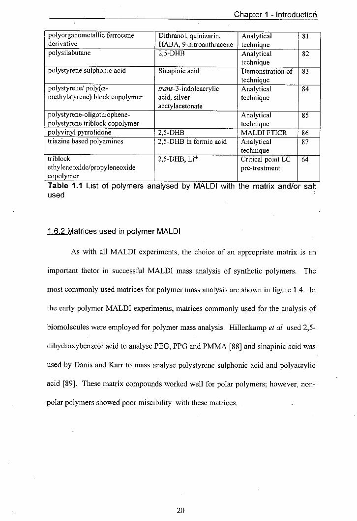
Table 1.1 List of polymers analysed by MALDI with the matrix and/or salt used
1.6.2 Matrices used in polymer MALDI
As with all MALDI experiments, the choice of an appropriate matrix is an
important factor in successful MALDI mass analysis of synthetic polymers. The
most commonly used matrices for polymer mass analysis are shown in figure 1.4. In
the early polymer MALDI experiments, matrices commonly used for the analysis of
biomolecules were employed for polymer mass analysis. Hillenkamp et al. used 2,5-
dihydroxybenzoic acid to analyse PEG, PPG and PMMA [88] and sinapinic acid was
used by Danis and Karr to mass analyse polystyrene sulphonic acid and polyacrylic
acid [89]. These matrix compounds worked well for polar polymers; however, non-
polar polymers showed poor miscibility with these matrices.
NO
Chapter 1 - Introduction
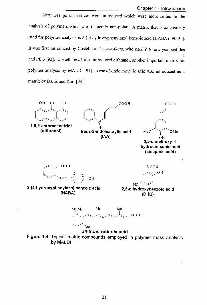
New less polar matrices were introduced which were more suited to the
analysis of polymers which are frequently non-polar. A matrix that is extensively
used for polymer analysis is 2-(-4 hydroxyphenylazo) benzoic acid (HABA) [90,91].
It was first introduced by Costello and co-workers, who used it to analyse peptides
and PEG [92]. Costello et al. also introduced dithranol, another important matrix for
polymer analysis by MALDI [91]. Trans-3-indoleacrylic acid was introduced as a
matrix by Danis and Karr [93].
OH OH OH
I ,8,9-anthracenetriol (d ith ranol)
COOH
C" J trans-3-indoleacrylic acid
(IAA)
COOH
Me 0 0 Me
3,5-dimethoxy-4-hydrocinnamic acid
(sinapinic acid)
COO H
NN OH
2-(4-hydroxyphenylazo) benzoic acid (HABA)
COOH
)OH
HO 2,5-dihydroxybenzoic acid
(DHB)
Me Me Me Me
COOH
Me
all-trans-retinoic acid Figure 1.4 Typical matrix compounds employed in polymer mass analysis
by MALDI
21
Chapter 1 - Introduction
1.6.3 MALDI mass analysis of polydisperse polymers
It has been noted that there can be discrepancies between average molecular
mass values obtained by MALDI and those obtained by other techniques [94]. There
is generally good agreement between MALDI and other techniques in the mass
analysis of monodisperse polymer samples [95]; however, mass discrimination has
been observed in the mass analysis of polydisperse polymer by MALDI in
comparison with other techniques. Several studies of the mass discrimination
phenomenon have been reported [94,96,97,98,99]. Perhaps the most complete and
extensive of these is the work published by Schriemer and Li [100,101]. Their work
examined sample preparation and desorption/ionisation [100] issues as well as
instrumental issues [101]. Some of the most significant factors in the analysis of
polydisperse polymer samples by MALDI appear to be the lack of high-mass
sensitivity of most commonly used detector systems [100] and more efficient
desorption of lower-mass polymers. Longer chain length polymers are more likely to
dimerise which leads to loss of signal intensity of the monomer [101].
1.6.3.1 Solutions to the polydisperse polymer analysis problem
The most commonly used method for overcoming the problems of
polydisperse MALDI analysis is chromatographic pre-treatment of the polymer
sample [102]. The separation technique of choice is usually size exclusion
chromatography (SEC), also called gel permeation chromatography (GPC). In
experiments of this type eluent samples are taken at various elution times and
MALDI mass analysed [103,104,105]. These eluent samples consist of a virtually
22
Chapter 1 - Introduction
monodisperse polymer distribution. In this way MALDI can be used as an absolute
mass detector for GPC. More traditional GPC detection systems need to be
calibrated with model polymer compounds and can therefore only give relative
molecular weight information. Furthermore, MALDI mass spectrometry can also
yield repeat-unit and endgroup mass information. The combination of MALDI with
GPC therefore is a powerful analytical tool which overcomes some of the main
weaknesses of the two constituent techniques, i.e. MALDI's difficulty in coping with
polydisperse samples and GPC's reliance on model compounds for calibration.
Current developments are focusing on automating the interface between the two
techniques [75,106,1 07].
1.6.4 Other polymer MALDI studies
A noteworthy demonstration of the high-mass analysis capacity of MALDI
was recently given by Schriemer and Li, when they mass analysed monodispersé
polystyrene samples of up to 1.5 MDa using MALDI time-of-flight mass
spectrometry [108]. The same group also used polystyrene mass analysis to
demonstrate the mass resolving power of a time-lag focusing mass spectrometer,
with polystyrene oligomers being resolved at masses over 50 kDa [72].
An area of polymer mass analysis that has generated considerable interest is
the attachment of metal ions to polymers to form adducts [109,110,111]. Metal ion
attachment issues will be discussed in some detail in chapters 5 and 6.
23
Chapter 1 - Introduction
1.7 References
F. Hillenkamp, mt. I Mass Spectrom. Ion Proc., 169, R9-R1 1 (1997) M. Yamashita and J. B. Fenn, I Phys. Chem., 88, 4451-4459 (1984) F. Hillenkamp and M. Karas, Anal. Chem., 60, 2299-2301 (1988) K. Tanaka, H. Waki, Y. Ido, S. Akita, Y. Yoshida and T. Yoshida, Rapid Commun. Mass Spectrom., 2,151-153 (1988)
[5] J. B. Williams, A. I. Gusev and D. M. Hercules, Macromolecules, 29, 8144- 8150(1996)
144- 8150(1996) M. R. Chevrier and R. J. Cotter, Rapid Commun. Mass Spectrom., 5, 611-617 (1991) R. C. Beavis and B. T. Chait, Rapid Commun. Mass Spectrom., 3, 43 6-43 9 (1989) R. C. Beavis and B. T. Chait, Rapid Commun. Mass Spectrom., 3, 233-237 (1989) S. Berkenkamp, C. Menzel, M. Karas and F. Hillenkamp, Rapid Commun. Mass Spectrom., 11, 1399-1406 (1997) M. Sadeghi, Z. Olumee, X. D. Tang, A. Vertes, Z. X. Jiang, A. J. Henderson, H. S. Lee and C. R. Prasad, Rapid Commun. Mass Spectrom., 11, 393-397 (1997) R. C. Beavis and B. T. Chait, Anal. Chem., 62,1836-1840 (1990) R. Knochenmuss, V. Karbach, U. Wiesli, K. Breuker and R. Zenobi, Rapid Commun. Mass Spectrom., 12, 529-534 (1998) B. Stahl, M. Steup, M. Karas and F. Hillenkamp, Anal. Chem., 63,1463-1466 (1991) B. Spengler, Y. Pan and R. J. Cotter, Rapid Commun. Mass Spectrom., 4, 99-102(1990) U. Bahr, A. Deppe, M. Karas and F. Hillenkamp, Anal. Chem., 64, 2866-2869 (1992) V. S. K. Kolli and R. Orlando, Rapid Commun. Mass Spectrom., 10, 923-926 (1997) C. G. de Koster, M. C. Duursma, G. J. v. Rooij, R. M. A. Heeren and J. J. Boon, Rapid Commun. Mass Spectrom., 9, 957-962 (1995) M. Guilhaus, I Mass Spectrom., 30, 1519-1532 (1995) A. Ingendoh, M. Karas, F. Hillenkamp and U. Giessmann, mt. I Mass Spectrom. Ion Proc., 131, 345-354 (1994) B. A. Mamyrin, mt. I Mass Spectrom. Ion Proc., 131, 1-19 (1994) W. C. Wiley and I. H. McLaren, Rev. Sci. Instrum., 67, 1150-1157 (1955) M. L. Vestal, P. Juhasz and S. A. Martin, Rapid Commun. Mass Spectrom., 9, 1044-1050 (1995) R. M. Whittal and L. Li, Anal. Chem., 67, 1950-1954 (1995) S. M. Colby, T. B. King and J. P. Reilly, Rapid Commun. Mass Spectrom., 8, 865-868 (1994)
IM
Chapter 1 - Introduction
R. S. Brown and J. J. Lennon, Anal. Chem., 67, 1998-2003 (1995) A. Bencsura and A. Vertes, Chem. Phys. Lett., 247, 142-148 (1995) A. Bencsura, V. Navali, M. Sadeghi and A. Vertes, Rapid Commun. Mass Spectrom., 11, 679-682 (1997) E. Lehmann, R. Knochenmuss and R. Zenobi, Rapid Commun. Mass Spectrom., 11, 1483-1492 (1997) H. Ehring, M. Karas and F. Hillenkamp, Org. Mass Spectrom., 27, 472-480 (1992) P. -C. Liao and J. Allison, J Mass Spectrom., 30, 408-423 (1995) I. A. Mowat, R. J. Donovan and R. R. Maier, Rapid Commun. Mass Spectrom., 11,89-90 (1997) B. H. Wang, K. Dreisewerd, U. Bahr, M. Karas and F. Hillenkamp, J Am. Soc. Mass Spectrom., 4, 393-398 (1993) A. -M. Hoberg, D. Haddleton and P.J. Derrick, Eur. Mass Spectrom., 3, 471-473 (1997) R Knochenmuss, F. Dubois, M. J. Dale and R. Zenobi, Rapid Commun. Mass Spectrom., 10, 871-877 (1996) J. W. Nicholson, The Chemistry of Polymers, The Royal Society of Chemistry, Cambridge, UK (1991) R. T. Morrison and R. N. Boyd, Organic Chemistry, 5th Ed., Allyn and Bacon Inc., Massachusetts, USA (1987) Transcript of product presentation by Viscotek (Unit 2, Lennox Mall, Lister Road, Basingstoke, Hampshire, RG22 4DF UK), April 1998 K. J. Wu and R. W. Odom, Anal. Chem., 70, 456 A-461 A (1998) C. A. Jackson and W.J. Simonsick, Current Opinion in Solid State and Materials Science, 2, 661-667 (1997) B. Thomson, K. Suddaby, A. Rudin and G. Lajoie, Eur. Polym. J, 32, 239-256 (1996) Polymer Laboratories Ltd, Church Stretton, Shropshire, UK. V. Schädler, J. Spickermann, H. J. Räder and U. Wiesner, Macromolecules, 29, 4865-4870 (1996) S. Coca, C. B. Jasieczek, K. L. Beers and K. Matyjaszewski, I Polym. Sci. Part A, 36, 1417-1424 (1998) H. Mandal and A. S. Hay, Polymer, 38, 6267-6271 (1997) J. C. Blais, M. Tessier, G. Bolbach, B. Remaud, L. Rozes, J. Guittard, A. Brunot, E. Maréchal and J. C. Tabet, mt. I Mass Spectrom. Ion Proc., 144, 131-138 (1995) H. S. Sahota, P. M. Lloyd, S. G. Yeates, P. J. Derrick, P. C. Taylor and D. M. Haddleton, I Chem. Soc., Chem. Commun., 2445-2446 (1994) P. J. Derrick, D. M. Haddleton, P. Lloyd, H. Sahota, P. C. Taylor and S. G. Yeates, Abs. Papers. Am. Chem. Soc., 208, No. Pt2, 271-Poly (1994) H. Pasch, R. Unvericht and M. Resch, Angew. Makromol. Chem., 212, 191-200 (1993) S. C. Hamilton, J. A. Semlyen and D. M. Haddleton, Polymer, 39, 3241-3252 (1998)
25
Chapter 1 - Introduction
Y. Ding and A. S. Hay, I Polym. Sci. Part A, 36, 5019-5026 (1998) M. R. Leduc, W. Hayes and J. M. J. Frechet, I Polym. Sci. Part A, 36, 1-10 (1998) L. Latourte, J. C. Blais and J. C. Tabet, Anal. Chem., 69, 2742-2750 (1997) Y. F. Wang, M. Paveni, K. P. Chan, A. S. Hay, I. Polym. Sci., Part A, 34 213 5 - 2138
135- 2138 (1997) B. Thomson, Z. Wang, A. Paine, A. Rudin and G. Lajoie, I Am. Oil Chem. Soc., 72(l),11-15 (1995) Y. F. Wang, M. Paventi and A. S. Hay, Polymer, 38, 469-482 (1997) K. L. Walker, M. S. Kahr, C. L. Wilkins, Z. Xu and J. S. Moore, I Am. Soc. Mass Spectrom., 5,731-739(1994) R. Abate, A. Ballistreri, G. Montaudo, D. Garozzo, G. Impallomeni, G. Critchley and K. Tanaka, Rapid Commun. Mass Spectrom., 7, 1033-1036 (1993) E. Scamporrino, D. Vitalini and P. Mineo, Macromolecules, 29, 5520-5528 (1996) P. 0. Danis and D. E. Karr, Org. Mass Spectrom., 28, 923-925 (1993) C. A. Martinez and A. S. Hay, I Polym. Sci. Part A, 35, 1781-1798 (1997) P. 0. Danis, D.E. Karr, W. J. Simonsick Jr. and D. T. Wu, Macromolecules, 28, 1229-1228 (1995) G. Montaudo, M. S. Montaudo, C. Puglisi and F. Samperi, Rapid Commun. Mass Spectrom., 8, 981-984 (1994) G. Montaudo, M. S. Montaudo, C. Puglisi and F. Samperi, Anal. Chem., 66, 4366-4369 (1994) H. Pasch and K. Rode, I. Chrom. A, 699, 21-29 (1995) G. Montaudo, M. S. Montaudo,C. Puglisi, F. Samperi, N. Spassky, A. LeBorgne and M. Wisniewski, Macromolecules, 29, 6461-6465 (1996) J. B. Williams, A. I. Gusev and D. M. Hercules, Macromolecules, 29, 8144-8150(1996) G. Montaudo, M. S. Montaudo, C. Puglisi and F. Samperi, Rapid Commun. Mass Spectrom., 9, 1158-1163 (1995) St. Weidner, G. KUhn and U. Just, Rapid Commun. Mass Spectrom., 9, 697-702 (1995) S. Weidner, G. Kuehn, R. Decker, D. Roessner and J. Friedrich, I Polym. Sci. Part A, 36, 1639-1648 (1998) S. Weidner, G. Kuehn, B. Werthmann, H. Schroeder, U. Just, R. Borowski, R. Decker, B. Schwarz, I. Schmuecking and I. Seifert, I Polym. Sci. Part A, 35 2183-2192 (1997) W. Mormann, J. Walter, H. Pasch and K. Rode, Macromolecules, 31, 249-255 (1998) R. M. Whittal, D. C. Schriemer and L. Li, Anal. Chem., 69, 2734-2741 (1997) G. J. van Rooij, M. C. Duursma, C. G. de Koster, R. M. A. Heeren, J. J. Boon, P. J. W. Schuyl and E. R. E. van der Hage, Anal. Chem., 70, 843-850 (1998) H. M. Burger, H.-M. Muller, D. Seebach, K. 0. Börnsen, M. Schär and H. M. Widmer, Macromolecules, 26,4783-4790 (1993)
26
Chapter 1 - Introduction
M. W. F. Nielen, Anal. Chem., 70,1563-1568, (1998) T. Yalcin, D. C. Schriemer and L. Li, J Am. Soc. Mass Spectrum., 8,1220-1229(1997)
,1220- 1229(1997) S. J. Pastor and C. L. Wilkins, I Am. Soc. Mass Spectrum., 8, 225-233 (1997) H. Mandal and A. S. Hay,i Polym. Sci. PartA,36, 1911-1918 (1998) A. M. Belu, J. M. Desimone, R. W. Linton, G. W. Lange and R. M. Friedman, I Am. Soc. Mass Spectrum., 7, 11-24 (1996) M. Eggert and R. Freitag, J. Polym. Sci. A, Polym. Chem., 32, 803-813 (1994) P. Juhasz and C. E. Costello, Rapid Commun. Mass Spectrum., 7, 343-351 (1993) K. Matsumoto, H. Shimazu, H. Yamaoka, I Polym. Sci. Part A, 36, 225-231 (1998) P. 0. Danis, D. E. Karr, F. Mayer, A. Holle and C. H. Watson, Org. Mass Spectrum., 27, 843-845 (27) G. Wilczek-Vera, P. 0. Danis and A. Eisenberg, Macromolecules, 29, 403 6-4044(1996) M. A. Hempenius, B. M. W. Langeveld-Voss, J. A. E. H. van Haare, R. A. J. Janssen, S. S. Sheiko, J. P. Spatz, M. Moller and E. W. Meijer, JAm. Chem. Soc., 120, 2798-2804 (1998) G. J. van Rooij, M. C. Duursma, R. M. A. Heeren, J. J. Boon and C. G. de Koster, I Am. Soc. Mass Spectrum., 7, 449-457 (1996) D. Braun, R. Grahary and H. Pasch, Polymer, 37, 777-783 (1996) U. Bahr, A. Deppe, M. Karas and F. Hillenkamp, Anal. Chem., 64, 2866-2869 (1992) P. 0. Danis, D. E. Karr, F. Mayer, A. Holle and C. H. Watson, Org. Mass Spectrum., 27, 843-845 (1992) G. Montaudo, M. S. Montaudo, C. Puglisi and F. Samperi, Rapid Commun. Mass Spectrum., 8, 1011-1015 (1994) P. Juhasz and C. E. Costello, Rapid Commun. Mass Spectrum., 7, 343-351 (1993) P. Juhasz, C. B. Costello and K. Biemann, I Am. Soc. Mass Spectrum., 4, 399-409(1993) P. 0. Danis and D. E. Karr, Org. Mass Spectrum., 28, 923-925 (1993) K. Martin, J. Spickermann, H. J. Rader and K. Mullen, Rapid Commun. Mass Spectrum., 10, 1471-1474 (1996) P. M. Lloyd, K. G. Suddaby, J. E. Varney, E. Scrivener, P. J. Derrick and D. M. Haddleton, Eur. Mass Spectrum., 1, 293-300 (1995) J. Axelsson, E. Scrivener, D. M. Haddleton and P. J. Derrick, Macromolecules, 29, 8875-8882 (1996) R. S. Lehrle and D. S. Sarson, Rapid Commun. Mass Spectrum., 9, 91-92 (1995) B. C. Guo, H. Chen, H. Rashidzadeh and X. Liu, Rapid Commun. Mass Spectrum., 11, 781-785 (1997) H. Rashidzadeh and B. C. Guo, Anal. Chem., 70, 131-135 (1998) D. C. Schriemer and L. Li, Anal. Chem., 69, 4169-4175 (1997)
27
Chapter 1 - Introduction
D. C. Schriemer and L. Li,Anal. Chem., 69,4176-4183 (1997) K. K. Murray, Mass Spectrom. Reviews, 16, 283-299 (1997) M. S. Montaudo, C. Puglisi, F. Samperi and G. Montaudo, Macromolecules, 31 3839-3845 (1998) M. W. Nielen and S. Malusha, Rapid Commun. Mass Spectrom., 11, 1194-1204 (1997) M. S. Montaudo, C. Puglisi, F. Samperi, G. Montaudo, Rapid Commun. Mass Spectrom., 12, 519-528 (1998) C. E. Kassis, J. M. DeSimone, R. W. Linton, E. B. Remsen, G. W. Lange and R. M. Friedmann, Rapid Commun. Mass Spectrom., 11, 1134-1138 (1997) X. Fei and K. K. Murray, Anal. Chem., 68, 3555-3560 (1996)
[108]D. C. Schriemer and L. Li, Anal. Chem., 68, 2721-2725 (1996) I. A. Mowat and R. J. Donovan, Rapid Commun. Mass Spectrom., 9, 82-90 (1995) M. J. Deery, K. R. Jennings, C. B. Jasieczek, D. M. Haddleton, A.T. Jackson, H. T. Yates and J. H. Scrivens, Rapid Commun. Mass Spectrom., 11, 57-62 (1997) C. K. L. Wong and T. W. D. Chan, Rapid Commun. Mass Spectrom., 11, 513-519(1997)
28
Chapter 2 - Instrumentation
Chapter 2— Instrumentation
2.1 Introduction
The experimental aspects of the research carried out will be discussed in two
chapters. The first chapter will deal with the instrumental set-up used and the second
chapter will deal with sample preparation.
The mass spectrometer described in this report was designed and constructed
in the Chemistry Department at The University of Edinburgh [1,2]. The instrument
was originally designed as a MALDI time-of-flight mass spectrometer, equipped
with a coaxial linear reflectron and a microchannel plate detector [1,2]. The original
design of the MALDI TOF mass spectrometer is illustrated in figure 2.1. Over the
course of the work described here, a number of - changes were made to the mass
spectrometer. The overall length of the flight tube was extended from 50 cm to 83
cm. The flight tube extension brought several advantages, improving mass separation
and allowing the installation of an in-line detector in addition to the original
reflectron detector. The addition of the in-line detector greatly enhanced the
versatility of the instrument, extending the mass range that could be studied and
making the study of metastable decay possible [3,4].
Another improvement to the mass spectrometer was the addition of a pulsed
deflection plate, allowing the removal of intense low-mass signals and therefore
4J
Chapter 2 - Instrumentation
improving sensitivity at higher masses. A schematic diagram of the extended mass
spectrometer is provided in figure 2.2.
Variable Neutral Density Filter
Nitrogen Steering Mirror Laser
Trigger
25cm Focal Length Lens
H 'Lll -
/ Circular (25mm) Extraction Cone Microchannel Plate Reflectron
Sample (ground) and Einzel ,' Detector (+1-Ito 20kV) Lens Holder (+/-Ito 20kV)
IBM compatible
O
I D~~,PIB
Link
50 cm total length
Figure 2.1 Full diagram of the apparatus prior to modification
Variable Neutral Density Filter
Nitrogen I Laser Steering Mirror
VII rigger Photodiode 25cm Focal Length Lens
mass gate (0 to 1 kV)
APulsed
I
7.- -
- - - -
Circular (25mm) ' Extraction Sample ,' cone Microchannel Plate
Holder (ground) and Einzel Detector Reflectron Microchannel Plate
(+/-Ito 20kV) Lens (+/-Ito 20kV) Detector
Digital I I Oscilloscope IBM compatible PC I
I I GPIB Link
83 cm total length
Figure 2.2 Full diagram of the experimental apparatus after the extension of the flight tube and the addition of a new detector and a mass gate.
30
Chapter 2 - Instrumentation
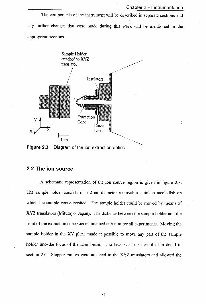
The components of the instrument will be described in separate sections and
any further changes that were made during this work will be mentioned in the
appropriate sections.
Sample Holder attached to XYZ translator
Insulators
01
Extraction Cone
Emzel
X Z Lens
1cm
Figure 2.3 Diagram of the ion extraction optics
2.2 The ion source
A schematic representation of the ion source region is given in figure 2.3.
The sample holder consists of a 2 cm-diameter removable stainless steel disk on
which the sample was deposited. The sample holder could be moved by means of
XYZ translators (Mitutoyo, Japan). The distance between the sample holder and the
front of the extraction cone was maintained at 6 mm for all experiments. Moving the
sample holder in the XY plane made it possible to move any part of the sample
holder into- the focus of the laser beam. The laser set-up is described in detail in
section 2.6. Stepper motors were attached to the XYZ translators and allowed the
31
Chapter 2 - Instrumentation
sample holder to be moved under computer control. For qualitative experiments, the
XY translators were moved manually. For quantitative experiments, on samples
produced by the aerosol method, (see section 3.3) the sample holder was moved by
the stepper motors, which were computer controlled. The stepper motors were
interfaced to a PC (XT, IBM) by means of an "isel" 3 axis steppermotor controller
fitted with an "isel" interface card (Isert-electronic, Eiterfeld, Germany). The
software for controlling the stepper motors was written in-house [5]. The sample
holder also acted as the repeller plate by means of which the ions were accelerated.
Two different high voltage power supplies to supply the repeller were used during
the course of this work, depending on the experiment. For work requiring low
extraction potentials, and delayed extraction experiments, a PS350 power supply
(Stanford Research Systems Inc.) with a maximum output voltage of 5 kV was used.
For all other experiments a home built power supply capable of delivering up to
20 kV was used. Either positive or negative ions could be extracted. For positive ion
extraction, the repeller was held at a positive potential while for negative ion
extraction the repeller voltage had to be negative. The extraction cone and the Einzel
lens of the ion optics were grounded for all experiments described in this thesis.
2.3 Time-of-flight mass analyser
The simplest time-of-flight mass analyser is a linear time-of-flight tube with a
detector at one end and an ion source at the other. The extreme simplicity, and hence
low cost and robustness, is one of the factors that make time-of-flight mass analysis
an attractive technique. Other factors are the theoretically unlimited mass range and,
more specifically to MALDI, the fact that it is ideally suited to coupling with a
32

Chapter 2 - Instrumentation
pulsed ion source. A drawback of time-of-flight analysis is its comparatively low
resolution. The problems with resolution are exacerbated in MALDI by the fact that
ions may be produced with a considerable energy spread [6,7,8]. The spread of
kinetic energy of ions produced by MALDI leads to a spread in ion velocity and
hence peak broadening in time-of-flight spectra. Several strategies have been
developed to compensate for the kinetic energy spread. The most commonly used
strategies are delayed ion extraction [9] or the use of a reflectron [10]. The principles
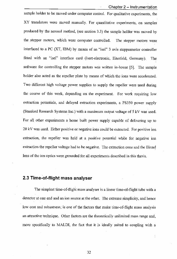
behind delayed extraction and reflectrons are laid out in detail in chapter 1. Initially
the instrument used for the work in this thesis was 50 cm long and equipped with a
reflectron and a microchannel plate detector (see fig. 2.4). Later, the flight tube was
extended by 33 cm and a second detector was added at the end of the reflectron
section, allowing the instrument to function both as a linear and as a reflectron time-
of-flight mass spectrometer (see figure 2.5).
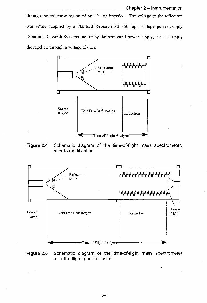
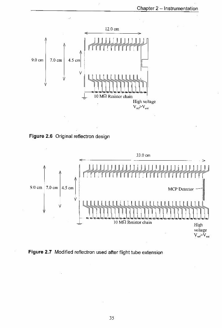
2.3.1 Reflectron Desian
Both of the reflectrons used were simple one stage gridded reflectrons. The
reflectron originally used and the reflectron installed during the flight tube extension
are shown in figure 2.6 and figure 2.7, respectively. The gridded front face of the
reflectron was grounded. The voltage to each lens element was increased, through a
resistor chain, up to a maximum voltage at the rear of the reflectron that exceeded the
voltage of the repeller in the source. The back plate in the original reflectron design
(fig. 2.6) was a solid plate. The redesigned back-plate consisted of a grid, which was
necessary to allow operation of the instrument in the linear mode. For operation in
the linear mode no voltage was supplied to the reflectron, allowing ions to travel
33
Chapter 2 - Instrumentation
through the reflectron region without being impeded. The voltage to the reflectron
was either supplied by a Stanford Research PS 350 high voltage power supply
(Stanford Research Systems Inc) or by the homebuilt power supply, used to supply
the repeller, through a voltage divider.
' _Reflectron MCP
Source Region Field Free Drift Region
Reflectron
Time-of-Flight Analyser
Figure 2.4 Schematic diagram of the time-of-flight mass spectrometer, prior to modification
,- Reflectron MCP
Source Region
Field Free Drift Region Reflectron Linear MCP
Time-of-Flight Analyser
Figure 2.5 Schematic diagram of the time-of-flight mass spectrometer after the flight tube extension
34
Chapter 2 - Instrumentation
12.0 cm
9.0 cm 7.0 cm 4.5 cm
High voltage Vret>Vext
Figure 2.6 Original reflectron design
33.0 cm
9.0 cm 17.0 cm 4.5 cm MCP Detector — t
voltage Yref>\Iext
Figure 2.7 Modified reflectron used after flight tube extension
35
Chapter 2 - Instrumentation
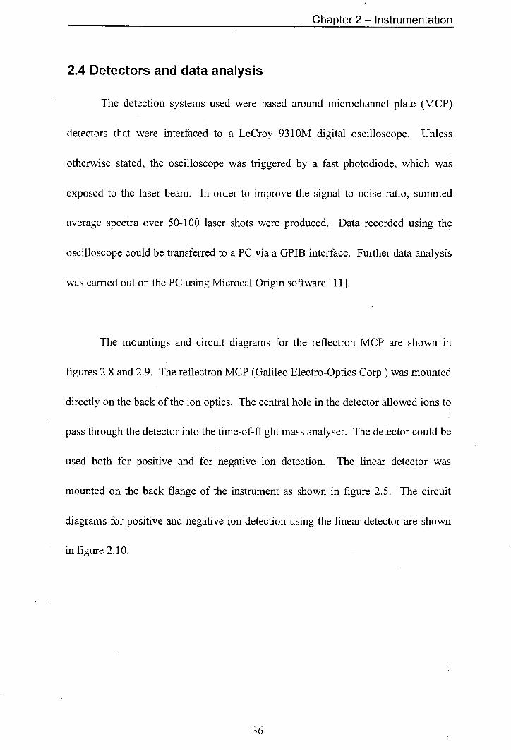
24 Detectors and data analysis
The detection systems used were based around microchannel plate (MCP)
detectors that were interfaced to a LeCroy 9310M digital oscilloscope. Unless
otherwise stated, the oscilloscope was triggered by a fast photodiode, which was
exposed to the laser beam. In order to improve the signal to noise ratio, summed
average spectra over 50-100 laser shots were produced. Data recorded using the
oscilloscope could be transferred to a PC via a GPIB interface. Further data analysis
was carried out on the PC using Microcal Origin software [11].
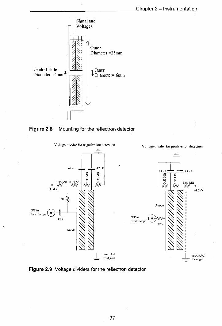
The mountings and circuit diagrams for the reflectron MCP are shown in
figures 2.8 and 2.9. The reflectron MCP (Galileo Electro-Optics Corp.) was mounted
directly on the back of the ion optics. The central hole in the detector allowed ions to
pass through the detector into the time-of-flight mass analyser. The detector could be
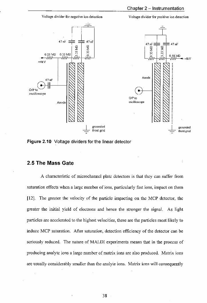
used both for positive and for negative ion detection. The linear detector was
mounted on the back flange of the instrument as shown in figure 2.5. The circuit
diagrams for positive and negative ion detection using the linear detector are shown
in figure 2.10.
36
Chapter 2 - Instrumentation
Signal and Voltages.
Outer Diameter =25mm
Central Hole 1Inner Diameter =4mm Diameter= 6mm
Figure 2.8 Mounting for the reflectron detector
Voltage divider for negative ion detection Voltage divider for positive ion detection
+1
OfPto oscilloscope \_
147 n
I rfl n .n
Anode
0/P to oscilloscope
50 Q I
47 nF
3.66 M13
-4.5kV
grounded front grid
grounded - front grid
Figure 2.9 Voltage dividers for the reflectron detector
37.
Chapter 2 - Instrumentation
Voltage divider for negative ion detection Voltage divider for positive ion detection
47nF
0.25MQ CD
±4kV
47nF
OF- c
en en en en
47 47 nF
-4kv
Anode 47 nF
0/P to oscilloscope
0/P to
Anode oscilloscope
grounded grounded front grid
front grid
Figure 2.10 Voltage dividers for the linear detector
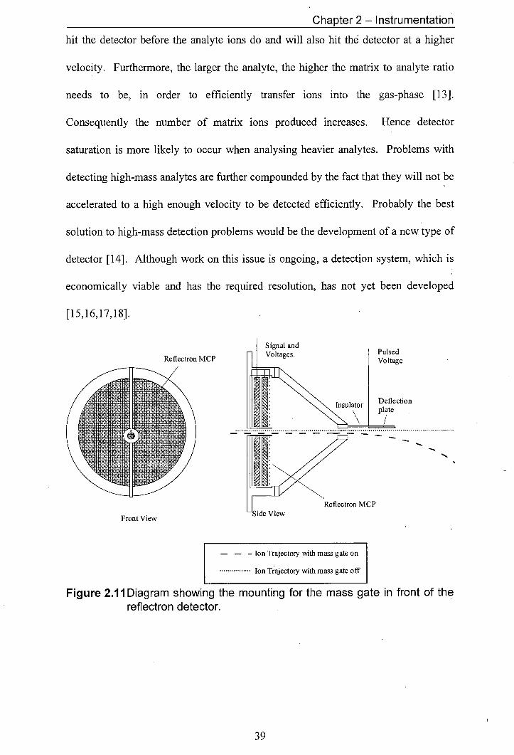
2.5 The Mass Gate
A characteristic of microchannel plate detectors is that they can suffer from
saturation effects when a large number of ions, particularly fast ions, impact on them
[12]. The greater the velocity of the particle impacting on the MCP detector, the
greater the initial yield of electrons and hence the stronger the signal. As light
particles are accelerated to the highest velocities, these are the particles most likely to
induce MCP saturation. After saturation, detection efficiency of the detector can be
seriously reduced. The nature of MALDI experiments means that in the process of
producing analyte ions a large number of matrix ions are also produced. Matrix ions
are usually considerably smaller than the analyte ions. Matrix ions will consequently
38
Front View View
Reflectron MCP Pulsed Voltage
Signal and Voltages.
Reflectron MCP
ChaDter 2 - Instrumentation
hit the detector before the analyte ions do and will also hit th6 detector at a higher
velocity. Furthermore, the larger the analyte, the higher the matrix to analyte ratio
needs to be, in order to efficiently transfer ions into the gas-phase [13].
Consequently the number of matrix ions produced increases. Hence detector
saturation is more likely to occur when analysing heavier analytes. Problems with
detecting high-mass analytes are further compounded by the fact that they will not be
accelerated to a high enough velocity to be detected efficiently. Probably the best
solution to high-mass detection problems would be the development of a new type of
detector [14]. Although work on this issue is ongoing, a detection system, which is
economically viable and has the required resolution, has not yet been developed
[15,16,17,18].
- - - Ion Trajectory with mass gate on
.Ion Trajectory with mass gate off
Figure 2.11 Diagram showing the mounting for the mass gate in front of the reftectron detector.
39

Chapter 2 - Instrumentation
Detector saturation caused by low-mass ions can be overcome by the use of a
mass gate. A mass gate is a device that deflects ions of a selected mass but allows
other ions to pass unhindered. The simplest mass gates consist of a deflection plate
or a pair of deflection plates, mounted parallel to the ion flight path in the field free
drift region of the mass spectrometer. As the ions that are to be deflected approach
the deflection plate a potential is applied to the plate; consequently the ion packet is
pushed onto a different trajectory. This change in direction results in a collision with
the sides of the flight tube. When an ion packet that is to be detected approaches the
deflector plates, the plates are switched to ground, allowing the ions to continue
without deflection. The simple deflector plate mass gate is very effective as a means
of removing low-mass signals from a time-of-flight spectrum and hence improving
detection efficiency of higher mass ions. More sophisticated ion gates have been
designed and used for the selection of ions of a single mass, such as the Bradbury-
Nielsen type ion gate [19]. These more elaborate devices are required where an ion
of a single mass needs to be selected e.g. when conducting tandem mass
spectrometry experiments. For the purposes of the work conducted in this research,
namely to extend the mass range over which the instrument could efficiently be used,
a simple deflector plate assembly was sufficient. The addition of an ion gate capable
of selecting a single mass peak would be a worthwhile avenue to, explore in future
work on this instrument.
The mass gate used was a single deflector plate, to which a high voltage pulse
was applied. The deflector plate was mounted in the field free drift region of the
mass spectrometer, as illustrated in figure 2.11. The high voltage switch and pulse
generator were built in-house. The high voltage switch was triggered by the pulse
Chapter 2 - Instrumentation
generator, which in turn was triggered from the synchronous output of the laser. The
high voltage was supplied by a Brandenburg power supply (model 475R) and was
typically +500 V. The high voltage pulse produced had a rise time of less than 50 ns.
The power to the pulser and high voltage switch was provided by a dual tracking dc
power supply (Topward Electric Instruments Co., Ltd, model tps-4000).
2.5.1 Illustration of the effectiveness of the mass gate
In order to demonstrate the performance of the mass gate several experiments
were carried out. A po1yropylene glycol) (PPG) sample (average molecular weight
ca 1000 Da) was prepared with dithranol as the matrix and LiC1 as the doping salt.
The sample was made up using the aerosol method described in section 3.3.3. The
effects of different gate voltages and gate pulse lengths were investigated. The gate
pulse length is taken as the duration of the high voltage pulse applied to the
deflection plate of the mass gate. The high voltage pulse was triggered on the
synchronous output of the laser and was timed so that the high voltage was applied at
the same time as the laser struck the sample holder. It was determined, that a pulse
voltage of +500 V was sufficient to deflect low-mass ions. The results of two
experiments are presented in figures 2.12 and 2.13.
The traces shown in figure 2.12 were recorded using a source repeller voltage
of 12 W. The spectrum shown in figure 2.12 (d) was obtained without the use of the
mass gate. All peaks with flight times above 12[is are due to lithium adducts of PPG
oligomers. The peaks below 12 ts are due to matrix species and metal ions. The
signal below 2 ts is due to noise pick up from the firing of the laser. The group of
41
Chapter 2 - Instrumentation
peaks at 7.5 ts is due to protonated and lithiated matrix. Further investigation
showed that the matrix peaks in the spectrum recorded without the mass gate were
off scale and are actually ca 50 to 100 times as intense, as they appear. The use of
the mass gate can be seen to remove low-mass ions from time-of-flight spectra (see
figures 2.12 (a) to (c)). In all spectra recorded with the mass gate on, the low-mass
peaks below 5 ts are no longer seen. By increasing the length of time that the gate is
left on, ions of increasingly larger masses are deflected and hence fewer peaks appear
in the mass spectra.
Little difference in the signal intensity of the polymer ions is seen whether the
mass gate is switched on or off. This is best illustrated by comparing figure 2.12 (d)
with figure 2.12 (c). The fact that the polymer signal intensity only increase a little
when the mass gate is employed shows that under the experimental conditions
employed little or no detector saturation occurred.
It is noteworthy, that a large peak is observed at 7.5 is in figures 2.12 (a) and
2.12 (b), despite the fact that other ions in that mass region have been deflected. The
species that are not affected by the mass gate are neutrals formed from the lithium
and sodium adducts of the matrix. The neutral nature of the species detected at
7.5 ts in figs 2.12 (a) and 2.12 (b) was confirmed, by switching on the reflectron and
using the linear detector to observe what passed through the reflectron. Only
uncharged species could pass through the reflectron. With the reflectron on, only the
peak at 7.5 jis was detected. The generation of neutrals under MALDI conditions
will be further discussed in chapter 5.
42
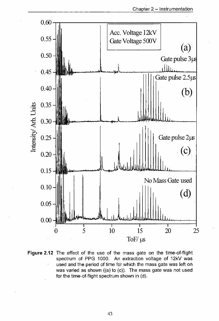
0.55
0.50
0.45
.' 0.35
0.30
0.25
0.20
0.15
0.10
Chaoter 2 - Instrumentation
0 5 10 15 20 25
ToF/ ps
Figure 2.12 The effect of the use of the mass gate on the time-of-flight spectrum of PPG 1000. An extraction voltage of 12kV was used and the period of time fdr which the mass gate was left on was varied as shown ((a) to (c)). The mass gate was not used for the time-of-flight spectrum shown in (d).
43
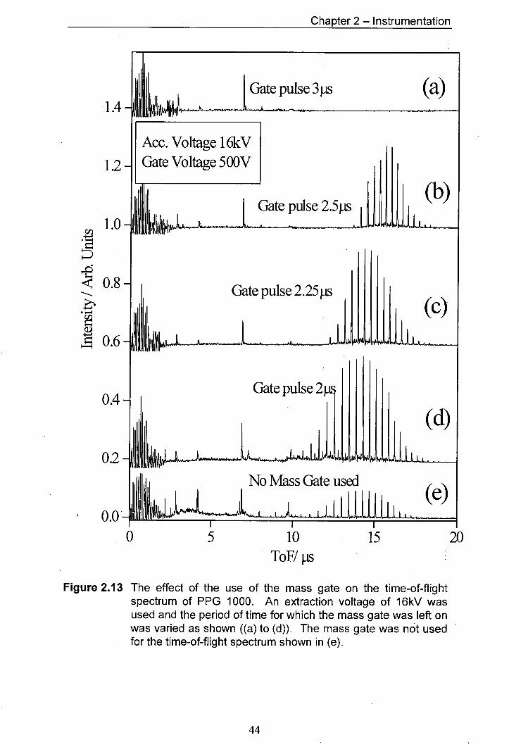
1.4
1.2
0.6
02
MI
Chapter 2 - Instrumentation
0 5 10 .15 20 ToF/ jts
Figure 2.13 The effect of the use of the mass gate on the time-of-flight spectrum of PPG 1000. An extraction voltage of 16kV was used and the period of time for which the mass gate was left on was varied as shown ((a) to (d)). The mass gate was not used for the time-of-flight spectrum shown in (e).
44
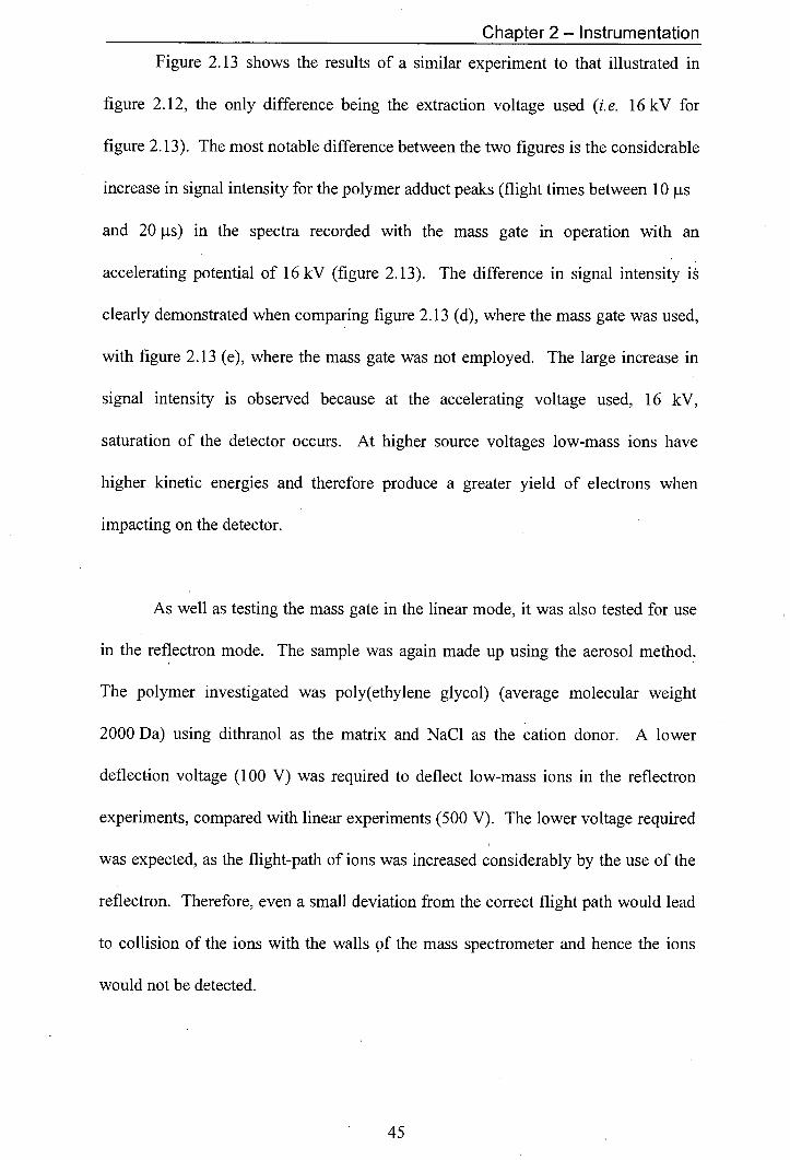
Chapter 2 - Instrumentation
Figure 2.13 shows the results of a similar experiment to that illustrated in
figure 2.12, the only difference being the extraction voltage used (i.e. 16 kV for
figure 2.13). The most notable difference between the two figures is the considerable
increase in signal intensity for the polymer adduct peaks (flight times between 10 is
and 20 is) in the spectra recorded with the mass gate in operation with an
accelerating potential of 16 kV (figure 2.13). The difference in signal intensity is
clearly demonstrated when comparing figure 2.13 (d), where the mass gate was used,
with figure 2.13 (e), where the mass gate was not employed. The large increase in
signal intensity is observed because at the accelerating voltage used, 16 kV,
saturation of the detector occurs. At higher source voltages low-mass ions have
higher kinetic energies and therefore produce a greater yield of electrons when
impacting on the detector.
As well as testing the mass gate in the linear mode, it was also tested for use
in the reflectron mode. The sample was again made up using the aerosol method.
The polymer investigated was poly(ethylene glycol) (average molecular weight
2000 Da) using ditbranol as the matrix and NaCl as the cation donor. A lower
deflection voltage (100 V) was required to deflect low-mass ions in the reflectron
experiments, compared with linear experiments (500 V). The lower voltage required
was expected, as the flight-path of ions was increased considerably by the use of the
reflectron. Therefore, even a small deviation from the correct flight path would lead
to collision of the ions with the walls of the mass spectrometer and hence the ions
would not be detected.
MCI
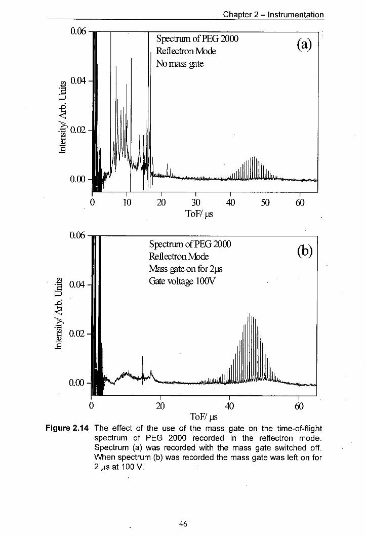
Chapter 2 - Instrumentation
A ( AVAJ
Spectnm of PEG 2000 (a) Reflectron Mode No mass gate
no
0 10 20 30 40 50 60 ToF! jis
M
0.04
LQ 0.02
0 20 40 60 ToF/ ps
Figure 2.14 The effect of the use of the mass gate on the time-of-flight spectrum of PEG 2000 recorded in the reflectron mode. Spectrum (a) was recorded with the mass gate switched off. When spectrum (b) was recorded the mass gate was left on for 2 .is at 100 V.
46
ChaDter 2 - Instrumentation
The results for the reflectron mass gate experiment are shown in figure 2.14.
An obvious difference between the reflectron and linear mode experiments is the
lower abundance of peaks in the low-mass region in the spectra recorded with the
mass gate on. In the reflectron experiment (figure 2.14 (b)) only two broad humps
centred at 10 ts and 17 ts, respectively, can be seen. The most likely origin of these
features is the detection of matrix ions, which were not deflected sufficiently to avoid
detection. The sharper feature observed in figure 2.14 (b), with a time-of-flight of
15 is, is switching noise from the high voltage switch of the mass gate.
Again, the analyte spectrum is enhanced by the use of the mass gate, as saturation
effects have been avoided.
2.6 Laser System
The laser used for all experiments in this thesis was a Lambda Physik
EMG 102 (Gottingen, Germany) excimer laser, running as a nitrogen laser. The gas
fill used was a mixture of 60 mbar of nitrogen with 940 mbar of helium. The laser
output produced from a 30 kV discharge was a 5 mJ pulse with a pulsewidth of
3.5 ns at a repetition rate of 6 Hz. The lasing wavelength was 337.1 rim. The beam
produced was steered into the source region of the mass spectrometer by two mirrors.
Owing to the large divergence of the beam only ca 25% of the light actually reached
the instrument. However, 1.2 mJ was still far in excess of the energy required for
MALDI experiments and the beam was further attenuated using a circular neutral
density filter. The use of the neutral density filter made it possible to adjust the laser
47
Chapter 2 - Instrumentation
energy smoothly. After attenuation the beam was focused onto the sample holder in
the source region of the instrument using a 25 cm focal length quartz lens. The angle
of incidence of the laser on the sample holder was 45°. The laser spot size and shape
on the sample holder was estimated using UV sensitive paper to be a teardrop shape
with a main axis length of ca 500 tm and a short axis length of ca 150-200 tm.
2.7 Pumping system
The whole mass spectrometer was pumped using one oil diffusion pump
(Edwards Diffstak 160) with a cryotrap. Edwards L9 diffusion pump fluid was used.
The diffusion pump was backed by a rotary pump (Edwards Speedivac ES200). The
diffusion pump could be isolated from the mass spectrometer by the use of a butterfly
valve. To accomplish the removal of the sample holder stage, the whole instrument
had to be brought up to atmospheric pressure which involved isolating the instrument
from the pumping system and gradually bringing it up to atmospheric pressure by
bleeding in nitrogen. Nitrogen was used to avoid the influence of water vapour and
thus facilitate the pumping down after sample loading. After sample loading, the
sample holder stage was refitted to the mass spectrometer and the system was
pumped down to operating pressure. Before the mass spectrometer could be pumped
by the diffusion pump, the system needed to be brought to a pressure of less than
5*1 02 mbar, using the rotary pump. When the rotary pump was used as a roughing
pump for the mass spectrometer, the diffusion pump was isolated. The base pressure
attainable using the diffusion pump was 5*1 08 mbar. Experiments could be
performed at a maximum pressure of 2* l06 mbar. It took ca 20min for the system
Chapter 2 - Instrumentation
to pump down to operating pressure after sample loading. The pressure in the
instrument was monitored using three pressure gauges. A Pirani gauge (Edwards
PRL 10) monitored the backing pressure of the diffusion pump. The pressure in the
mass spectrometer was measured by a Pirani gauge (Edwards PRL 10) and a Penning
gauge (Edwards CP25EK). All gauges were controlled via a Pirani Penning 1005
pressure gauge controller (Edwards).
2.8 Conclusion
This chapter has given a description of the instrumentation employed, in the
experimental work for this thesis. Changes made to the experimental set-up have
been discussed, including a detailed discussion of the introduction of a low-mass gate
for eliminating low-mass ions from mass spectra.
49
Chapter 2 - Instrumentation
29 References
I. A. Mowat and R. J. Donovan, Rapid Commun. Mass Spectrom., 9, 82-90 (1995) I. A. Mowat, R. J. Donovan and R. R. Maier, Rapid Commun. Mass Spectrom., 11, 89-90 (1997) S. Della-Negra and Y. Le Beyec, Anal. Chem., 57, 2035-2040 (1985) R. Kaufmann, D. Kirsch and B. Spengler, mt. .i Mass Spectrom. Ion Proc., 131, 355-385 (1994) Program written in QuickBasic by M. F. Snel and L. Hogg, not published. V. Bokelmann, B. Spengler and R. Kaufmann, Eur. Mass Spectrom., 1, 81-93 (1995) Y. Pan and R. J. Cotter, Org. Mass Spectrom., 27, 3-8 (1992) R. C. Beavis and B. T. Chait, Chem. Phys. Lett., 181, 479-484 (1991) W. C. Wiley and I. H. McLaren, Rev. Sci. Instrum., 67,1150-1157 (1955) B. A. Mamyrin, mt. i Mass Spectrom. Jon Proc., 131, 1-19 (1994) MicroCal Software Inc., One Roundhouse Plaza, Northampton, MA 01060, USA A. Westman, G. Brinkmalm and D. F. Barofsky, mt. J Mass Spectrom. Ion Proc., 169, 79-87 (1997) D. C. Schriemer and L. Li, Anal. Chem., 68, 2721-2725 (1996) D. C. Schriemer and L. Li, Anal. Chem., 69, 4176-4183 (1997) F. Dubois, R. Knochenmuss and R. Zenobi, mt. I Mass Spectrom. Ion Proc., 169, 89-98 (1997) U. Bahr, U. Rohling, C. Lautz, K. Strupat, M. Schurenberg and F. Hillenkamp, Int. I. Mass Spectrom. Ion Proc., 153, 9-21 (1996) G. C. Hilton, J. M. Martinis, D. A. Woliman, K. D. Irwin, L. L. Dulcie, D. Gerber, P. M. Gillevet and D. Twerenbold, Nature, 391, 672-675 (1998) D. C. Imrie, J. M. Pentney and J. S. Cottrell, Rapid Commun. Mass Spectrom., 9, 1293-1296 (1995) C. W. Stoermer, S. Gilb, J. Friedrich, D. Schooss and M. M. Kappes, Rev. Sci. Inst., 69, 1661- 1664 (1998)
50
Chapter 3 - Sample preparation
Chapter 3- Sample preparation
3.1 Introduction
Sample preparation is of key importance for successful MALDI mass
analysis. Without due attention being paid to sample preparation the results become
very scattered and irreproducible [1]. It has recently been shown that, through
careful sample preparation, narrow molecular fractions of polystyrene with average
molecular weights of up to 1.5 MDa can be mass analysed [2]. It is also known that
the resolution of mass spectra can be affected by sample preparation. In the analysis
of synthetic polymers, even the molecular weight distribution observed can vary with
different sample preparation regimes [3].
The work presented here has focused on the mass analysis of synthetic
polymers and this chapter will therefore deal with sample preparation for synthetic
polymers. For synthetic polymer mass analysis samples usually consist of a mixture
of three components, namely the polymer, a salt and the matrix. In this mixture, the
polymer is the analyte. The matrix absorbs the laser radiation which facilitates
transition of the analyte into the gas phase and plays a role in the ionisation process.
Polymers are usually detected in the form of metal cation polymer adducts and the
salt is added as a cation source for adduct formation with the polymer [4,5]. The
ratios between the three sample constituents are determined ethpirically and are
dependent on the nature of the sample constituents.
Chapter 3 - Sample preparation
A problem that has been reported and that was also observed in this work wa
poor shot to shot reproducibility of signal intensity [1]. This posed a significant
problem when quantitative studies were carried out. An example of an experiment
requiring good reproducibility is one in which the variation of one experimental
parameter is investigated, such as laser energy, extraction potential, etc. The work
described in this chapter details the development of a method of sample preparation
that improves shot to shot reproducibility and hence facilitates quantitative
experiments. This chapter is also intended to give a practical guide to sample
preparation for polymer MALDI.
3.2 Choice of matrix and salt
Over the years, many new MALDI matrices have been introduced, some of
which are very well suited to polymer analysis. Several matrices were used
successfully during this research. The matrices most commonly used are
summarised in Table 3.1. For the analysis of new types of polymers, all the matrices
were tried and the best one chosen for further work. A molar ratio of matrix to
polymer of between 40:1 and 500:1 was used for polymers with average molecular
weights of up to 20 kDa. Dithranol was used very successfully for low-mass
polymers up to ca 7000 Da. 2-(4-hydroxyphenylazo) benzoic acid (HABA) [6,7] and
3-3-indole acrylic acid (IAA) [8] were both used for analysing higher mass polymers
and copolymers. HABA and IAA gave rise to large signals from matrix species,
including multimers extending up to 1500 Da, making them a less suitable choice for
52

Chapter 3 - Sample preparation
low mass polymer analysis. All-trans-retinoic acid was used exclusively for
polystyrene analysis [9].
Name of Matrix Suitable Concentration Comments Solvents Range I g L 1
1,8,9-anthracenetriol THE 5-20 Good all round polymer matrix (Dithranol) very good for low mass
polymers 2-(4-hydroxyphenylazo) acetone, 5-20 Good for higher mass polymers benzoic acid (HABA) 1 ,4-dioxane >8kDa. Large signal associated
with matrix multimers 3-13-indole acrylic acid acetone 5-20 Suitable for polymer and (IAA) copolymer analysis all-trans-retinoic acid THF 20-50 Very good matrix for polystyrene
analysis Table 3.1 Summary of some commonly used matrices for polymer mass
analysis
For all experiments conducted, salt was added to the sample, to provide a
source of cations for attachment to the polymers. A variety of salts was used.
Although no hard and fast rules can be made as to which cation attaches most
efficiently it was found that for most polymers alkali metal-ions were suitable. Of
the alkali metals, lithium tended to give the most intense mass spectra. Although
alkali metal ions worked very well in most cases, other metal ions were also used for
polymer MALDI. Polystyrene, for example, forms adducts most readily using silver
or other transition metal ions [4,10]. The salts used in this work were the chlorides
of the alkali metals and AgCF3CO2 or AgNO3 as a silver ion source. The
trifluoroacetate of silver was chosen for two reasons; first it contains silver in the 1+
oxidation state and, second, this salt is readily soluble in tetrahydrofuran, which
facilitates the mixing of salt solution with matrix and polymer solutions. The amount
of salt added changed significantly for different sample preparation schemes and will
be dealt with in the following sections on sample deposition.
53
Chapter 3 - Sample preparation
3.3 Sample deposition
Three different sample deposition methods were employed during this work.
The first method will be referred to as the droplet method, where a micropipette was
used for depositing the sample on the sample holder [11 ]. The other two methods
involved using spray techniques for sample deposition. These will be referred to as
the electrospray and the aerosol method, respectively. For the electrospray method, a
fine spray was produced by drawing the sample through a hypodermic needle by
means of an applied electrical potential. In the case of the aerosol method, the sample
was deposited using an aerosol spray-gun. A summary of the advantages and
disadvantages of the droplet method and the two spray techniques is given in
table 3.2.
Techniques that rely on depositing droplets of sample solution onto the
sample holder are the most commonly used MALDI sample preparation methods.
The droplet method is useful as a qualitative technique, best suited to analysing a
large number of samples quickly or for finding the correct ratio between matrix, salt
and polymer. The droplet method was, however, found to be less suitable for
detailed quantitative work. The limitations of this type of sample preparation have
been recognised by several groups and alternative sample preparation techniques
have been suggested [1,12]. The primary problems with the sample spots produced
by the droplet method are the uneven surface and the limited size of the sample spot.
One of the factors giving rise to an inhomogeneous sample surface is that the solvent
evaporates more quickly at the edges of the droplet than at the centre. This can lead
54
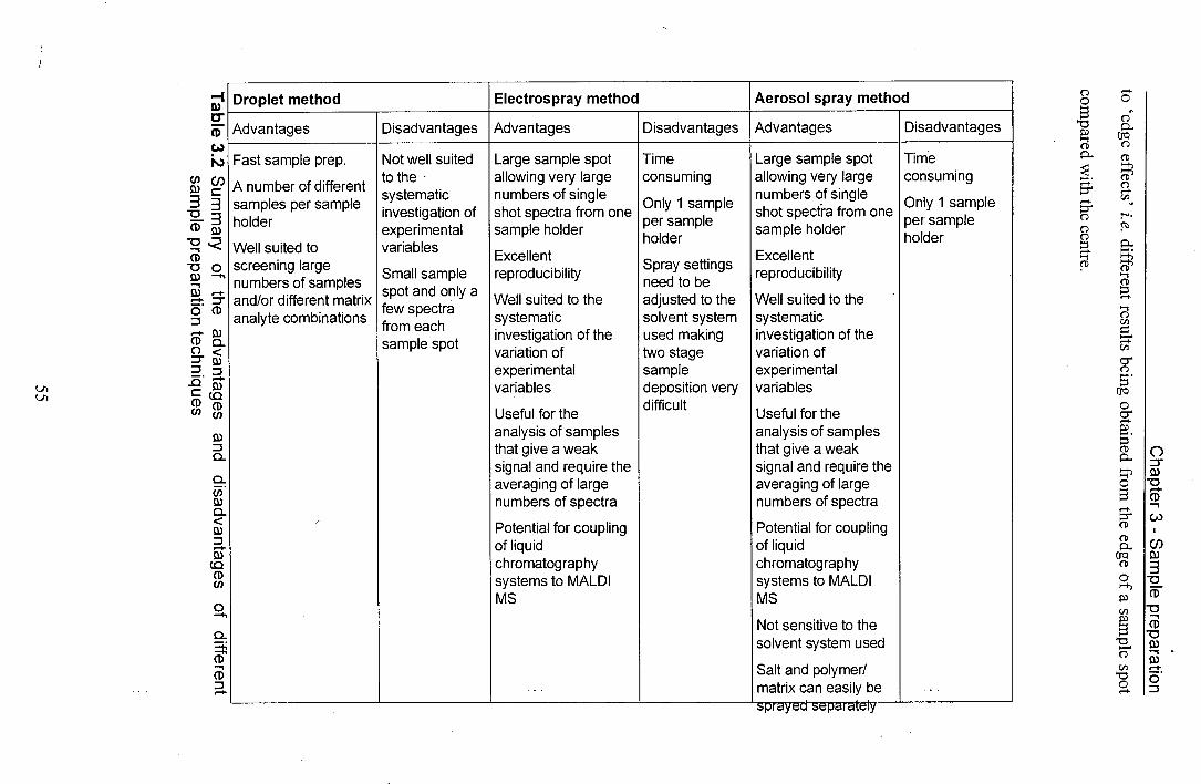
.JIJI CAY .CA %?.#VCAICA¼
Droplet method Electrospray method Aerosol spray method
Advantages Disadvantages Advantages Disadvantages Advantages Disadvantages
Fast sample prep. Not well suited Large sample spot Time Large sample spot Time
A number of different to the allowing very large consuming allowing very large consuming
samples per sample systematic numbers of single
Only 1 sample numbers of single Only 1 sample
holder investigation of shot spectra from one
per sample shot spectra from one per sample
experimental sample holder holder sample holder holder
Well suited to variables Excellent Excellent screening large Small sample reproducibility Spray settings reproducibility numbers of samples spot and only a
need to be and/or different matrix few spectra
Well suited to the adjusted to the Well suited to the analyte combinations from each
systematic solvent system systematic
sample spot investigation of the used making investigation of the variation of two stage variation of experimental sample experimental variables deposition very variables
Useful for the difficult
Useful for the analysis of samples analysis of samples that give a weak that give a weak signal and require the signal and require the averaging of large averaging of large numbers of spectra numbers of spectra
Potential for coupling Potential for coupling of liquid of liquid chromatography chromatography systems to MALDI systems to MALDI MS MS
Not sensitive to the solvent system used
Salt and polymer/ matrix can easily be
CD (pJ Isj
Cr,
33 CD )
Th CD 0 0 1
OCD
CD C). 0< - )
2. - C ca CD CD
a lei
0 -I
a
CD 1
CD
CD
0
Chapter 3 - Sample preparation
Derrick et al. proposed a sample preparation technique in which the matrix*
analyte mixture was deposited on the sample holder using an electrospray method
[1]. This work was repeated at The University of Edinburgh and it was found to
work well for samples where the matrix polymer and salt could be dissolved in the
same solvent. However, it was difficult to use two-stage sample deposition where
first a salt solution and then a matrix/analyte solution was sprayed onto the sample
holder. Problems arose when adjustments had to be made to the spray conditions
after the salt layer was sprayed, owing, to the different physical properties of the
aqueous salt solution, compared with the organic solvent used for the matrix and
analyte. It was difficult to optimise spray conditions for both layers, and this led to
poor sample quality. It was also an extremely time consuming method.
An alternative approach was developed. A spray-gun was used to coat the
sample holder first with a salt layer and then with the sample/matrix mixture. The
spray-gun technique was found to be less solvent dependent than the electrospray
technique. Using a spray-gun was also more straightforward, as it did not require the
design and construction of specific apparatus, unlike the electrospray technique.
The strength of the spray techniques was in quantitative work, for instance,
when the ratios of the sample components were kept constant, and other experimental
parameters, such as laser energy or the ion extraction field strength, were varied. As
a large sample spot with an even sample surface was produced it became possible to
collect a large number of spectra from the same sample holder, using a fresh section
of the sample for each laser shot. Each of these methods is discussed in some detail
below.
56
Chapter 3 - Sample preparation
3.3.1 The droplet method
The droplet method is a very simple technique for MALDI sample
preparation. It involves depositing a small droplet of sample solution on the sample
holder and leaving the solvent to evaporate. Most MALDI experiments described in
the literature involve this method of sample preparation.
A micropipette (Socorex, Switzerland) was used to spot the sample onto the
sample holder. The sample holder consisted of a 2 cm diameter stainless steel disk,
which had been thoroughly cleaned and polished. Sample deposition could be a one
or a two-stage process depending on the matrix and polymer used.
For the one-stage droplet deposition method, solutions were prepared of salt,
polymer and matrix and these were combined prior to sample deposition.
A 0.5 to 2 pL droplet of the polymer, analyte and salt mixture was then spotted
straight onto the sample holder by means of the micropipette, and the solvent was left
to evaporate. The quality of the sample spot that was produced using this method
varied, depending mostly on the surface tension of the solvents used. Droplets of
solutions with low surface tension spread out quickly over the sample holder and the
solvent evaporated very quickly, leading to an uneven sample surface and poor
reproducibility of MALDI mass spectra. However, it was often still possible to
obtain mass spectra from these sample spots from which valuable qualitative
information could be obtained.
57
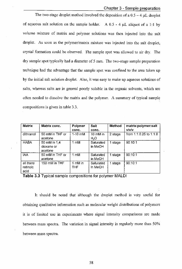
Chapter 3 - Sample preparation
The two-stage droplet method involved the deposition of a 0.5 - 4 p.L droplet
of aqueous salt solution on the sample holder. A 0.5 - 4 tL aliquot of a 1:1 by
volume mixture of matrix and polymer solutions was then injected into the salt
droplet. As soon as the polymer/matrix mixture was injected into the salt droplet,
crystal formation could be observed. The sample spot was allowed to air dry. The
dry sample spot typically had a diameter of 5 mm. The two-stage sample preparation
technique had the advantage that the sample spot was confined to the area taken up
by the initial salt solution droplet. Also, it was easy to make up aqueous solutions of
salts, whereas salts are in general poorly soluble in the organic solvents, which are
often needed to dissolve the matrix and the polymer. A summary of typical sample
compositions is given in table 3.3.
Matrix Matrix conc. Polymer Salt Method matrix:polymer:salt conc. conc. v/v/v
dithranol 50 mM in THF or 1-10 mm 10 mM in 2 stage from 1:1:0.25 to 1:1:8 acetone H20
HABA 50 mM in 1,4 1 mM Saturated 1 stage 90:10:1 dioxane or in MeOH acetone
IAA 50 mM in THE or 1 mM Saturated 1 stage 90:10:1 acetone in MeOH
all trans 150 mM in THF 1 mM in Saturated 1 stage 90:10:1 retinoic THE in MeOH
Table 3.3 Typical sample compositions for polymer MALDI
It should be noted that although the droplet method is very useful for
obtaining qualitative information such as molecular weight distributions of polymers
it is of limited use in experiments where signal intensity comparisons are made
between mass spectra. The variation in signal intensity is regularly more than 50%
between mass spectra.
58
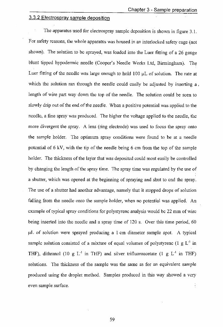
Chapter 3 - Sample preparation
3.3.2 Electrospray sample deposition
The apparatus used for electrospray sample deposition is shown in figure 3.1.
For safety reasons, the whole apparatus was housed in an interlocked safety cage (not
shown). The solution to be sprayed, was loaded into the Luer fitting of a 26 gauge
blunt tipped hypodermic needle (Cooper's Needle Works Ltd, Birmingham). The
Luer fitting of the needle was large enough to hold 100 p.L of solution. The rate at
which the solution ran through the needle could easily be adjusted by inserting a
length of wire part way down the top of the needle. The solution could be seen to
slowly drip out of the end of the needle. When a positive potential was applied to the
needle, a fine spray was produced. The higher the voltage applied to the needle, the
more divergent the spray. A lens (ring electrode) was used to focus the spray onto
the sample holder. The optimum spray conditions were found to be at a needle
potential of 6 kV, with the tip of the needle being 6 cm from the top of the sample
holder. The thickness of the layer that was deposited could most easily be controlled
by changing the length of the spray time. The spray time was regulated by the use of
a shutter, which was opened at the beginning of spraying and shut to end the spray.
The use of a shutter had another advantage, namely that it stopped drops of solution
falling from the needle onto the sample holder, when no potential was applied. An
example of typical spray conditions for polystyrene analysis would be 22 mm of wire
being inserted into the needle and a spray time of 120 s. Over this time period, 60
tL of solution were sprayed producing a 1 cm diameter sample spot. A typical
sample solution consisted of a mixture of equal volumes of polystyrene (1 g L 1 in
THF), dithranol (10 g L' in THF) and silver trifluoroacetate (1 g L 1 in THF)
solutions. The thickness of the sample was the same as for an equivalent sample
produced using the droplet method. Samples produced in this way showed a very
even sample surface.
59
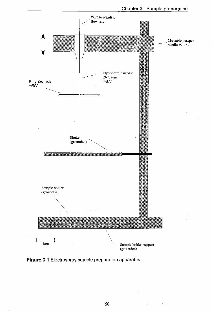
Chapter 3 - Sample preparation
Wire to regulate
Ring electrode +6kv
Shutter (grounded)
Sample holder (grounded)
1cm Sample holder support (grounded)
Figure 3.1 Electrospray sample preparation apparatus
Movable perspex needle mount

Chapter 3 - Sample preparation
0.O1
0.010
0.006
0.004
[IIIIIIS1
750 1000 1250 1500 1750 2000 2250 rn'z
Figure 3.2 Example of polystyrene mass spectrum produced using the electrospray sample preparation method. Dithranol was used as the matrix and AgCF3CO2 as the salt.
The reproducibility across samples was studied by collecting a series of
spectra from a sprayed sample. Polystyrene samples were used with an average
molecular weight of 1340 Da. A typical mass spectrum is shown in figure 3.2. In
the reproducibility experiment presented here, 13 spectra were collected. All spectra
were the summed averages of 50 single shot spectra. During data acquisition, the
sample holder was moved at a constant speed of 60 tm s' relative to the laser by
means of computer controlled stepper motors. This ensured that every laser pulse hit
a previously unused spot. The data were evaluated by making a comparison of the
area under the 12-mer peak of polystyrene in each spectrum collected. The
normalised results are presented in figure 3.3. As can clearly be seen, quite good
61
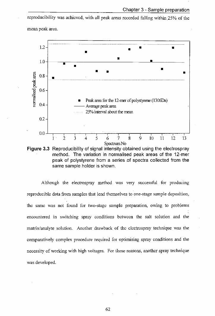
Chapter 3 - Sample preparation
reproducibility was achieved, with all peak areas recorded falling within 25% of the
mean peak area.
1.2
1.0
0.8
I 0.6
10.4
0.2
-------------------------------------------------------------------------------------------------------------------
U . .
I U
U U
. U • U
U -------------------------------------------------------------------------------------------------------------------
Peak area for the 12-mer of polystyrene (1306Da) Average peak area 25% interval about the nan
xi1 1 2 3 4 5 6 7 8 9 10 11 12 13
Spectrum No Figure 3.3 Reproducibility of signal intensity obtained using the electrospray
method. The variation in normalised peak areas of the 12-mer peak of polystyrene from a series .of spectra collected from the same sample holder is shown.
Although the electrospray method was very successful for producing
reproducible data from samples that lend themselves to one-stage sample deposition,
the same was not found for two-stage sample preparation, owing to problems
encountered in switching spray conditions between the salt solution and the
matrix/analyte solution. Another drawback of the electrospray technique was the
comparatively complex procedure required for optimising spray conditions and the
necessity of working with high voltages. For these reasons, another spray technique
was developed.
62
Chapter 3 - Sample preparation
3.3.3 The aerosol method
The spray gun used in these experiments was a modified thin layer
chromatography (TLC) spray gun. The solvent reservoir of the spray gun was
replaced with a 7 mL glass sample vial. The vial was attached to the spray gun by
means of the vial's plastic lid, which had been punctured to allow a tube, which was
attached to the spray gun nozzle, to be inserted into the vial. Compressed air was
used to produce the aerosol. As with the droplet technique, both single and two-stage
sample deposition could be used.
For two-stage sample preparation, 1.5 mL of salt solution (0.01 M in
deionised water) was sprayed onto a heated sample holder. The sample holder was
heated to aid the evaporation of the water. The total area sprayed was a circle of ca
5 cm diameter. The sample holder was at the centre of the spray circle and measured
2 cm in diameter. A uniform dry salt layer was deposited over the full area of the
sample holder. The sample holder was then allowed to cool to room temperature.
Once the sample holder had cooled, the second solution was sprayed onto the sample
holder. The solution sprayed consisted of 0.75 mL matrix solution (e.g. 10 g L
dithranol in THF) mixed with 0.75 mL of polymer solution (1 mM solution). The
matrix/polymer solution could be seen to wet the previously deposited salt layer
before the solvent evaporated, ensuring good mixing between all three sample
components. It was essential that the sample holder should be cold, as
decomposition/reaction of polymer molecules has been observed as a result of
spraying the second coat onto a hot substrate. The sample produced had a very
31
Chapter 3 - Sample preparation
homogenous surface and it was shown that a large number of spectra could be
recorded with very reproducible peak intensities (a spread of ca 25% around the
average). During data acquisition the sample holder was moved by stepper motor at
a speed of 60 tm s 1, ensuring that every single shot spectrum was collected from a
fresh part of the sample.
The reproducibility of the aerosol technique was tested in the same way as the
electrospray technique. The results are shown in figure 3.4. It should be noted that,
with this experiment, a two-stage sample preparation technique was used. As can be
seen, reasonable reproducibility was obtained, with all values falling within 25% of
the mean.
The aerosol technique was extremely robust and easy to use. It gave good
reproducibilty both for one and two-stage sample deposition. During the course of
this work, the aerosol technique was used for most experiments that required good
reproducibility. The technique also proved to be a useful tool when analysing
samples that only produced weak signal intensity as, owing to the large size of the
sample spot, it was possible to produce spectra averaged over several thousand laser
shots, with each single shot hitting a previously unused part of the sample surface.
By averaging over such a large number of shots, the signal-to-noise ratio could be
improved.
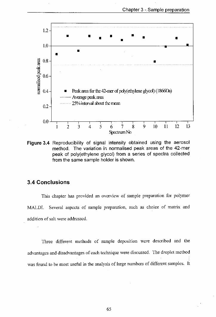
Chapter 3 -.Sample preparation
------------- ..... U
*'''"'I -----
U
-- -------
I *'"*''* ........ **
U
------- --- ------- ----- ** .... * ..... • • . • 1.0
U IN
1..................................................................................................
Peak area for the 42-nr of poly(ethylene glycol) (1866Da)
Average peak area
25% interval about the mean 0.2
1 2 3 4 5 6 7 8 9 10 11 12 13 SpectnirnNo
Figure 3.4 Reproducibility of signal intensity obtained using the aerosol method. The variation in normalised peak areas of the 42-mer peak of poly(ethylene glycol) from a series of spectra collected from the same sample holder is shown.
3.4 Conclusions
This chapter has provided an overview of sample preparation for polymer
MALDI. Several aspects of sample preparation, such as choice of matrix and
addition of salt were addressed.
Three different methods of sample deposition were described and the
advantages and disadvantages of each technique were discussed. The droplet method
was found to be most useful in the analysis of large numbers of different samples. It
1.2
65
Chapter 3 - Sample preparation
was, however, limited in its use for experiments requiring good shot-to-shot
reproducibility of signal intensity.
Two spray techniques were investigated, namely an electrospray and an
aersosol spray technique. The spray techniques were both seen to produce large
sample spots with very homogeneous sample surfaces. The reproducibilty of signal
intensity was shown to be good for both techniques. The good reproducibility meant
that these techniques are well suited as sample deposition techniques, when
conducting experiments where quantitative data are required. Both spray techniques
were useful for depositing samples in a one-stage approach. However, the
electrospray technique was found to be difficult to use for two-stage sample
deposition, whereas the aerosol technique was not subject to this restraint. The
aerosol technique was also found to be easier to use and more robust than the
electrospray technique. However, spray techniques may be too time consuming to be
used for the routine analysis of large numbers of samples.
Chapter 3 - Sample preparation
3.5 References
J. Axelson, A. Hoberg, C. Waterson, P. Myatt, G. L. Shield, J. Varney, D. M. Haddleton and P. J. Derrick, Rapid Commun. Mass Spectrom., 11, 209-213 (1997) D. C. Schriemer and L. Li, Anal. Chem., 68, 2721-2725 (1996) D. C. Schriemer and L. Li, Anal. Chem., 69, 4169-4175 (1997) I. A. Mowat and R. J. Donovan, Rapid Commun. Mass Spectrom., 9, 82-90 (1995) H. Rashidezadeh and B. C. Guo, J. Am. Soc. Mass Spectrom., 9, 724-730 (1998) G. Montaudo, M. S. Montaudo, C. Puglisi and F. Samperi, Rapid Commun. Mass Spectrom., 8, 1011-1015 (1994) P. Juhasz and C. E. Costello, Rapid Commun. Mass Spectrom., 7, 343-351 (1993) P. 0. Danis and D. E. Karr, Org. Mass Spectrom., 28, 923-925 (1993) K. L. Walker, M. S. Kahr, C. L. Wilkins, Z. Xu and J. S. Moore, J Am. Soc. Mass Spectrom., 5, 731-739 (1994)
M. J. Deery, K. R. Jennings, C. B. Jasieczek, D. M. Haddleton, A.T. Jackson, HT. Yates and J. H. Scrivens, Rapid Commun. Mass Spectrom., 11, 57-62 (1997) Ian A. Mowat, PhD Thesis, The University of Edinburgh (1995) R. R. Hensel, R. C. King and K. G. Owens, Rapid Commun. Mass Spectrom., 11, 1785-1793 (1997)
67
Chapter 4 - Analysis of high-mass polymers
Chapter 4- Analysis of high-mass polymers
4.1 Introduction
One of the aims of this research was to extend the mass range over which the
existing mass spectrometer was usable. Previously, the instrument was only
effective up to ca 5 kDa, for polymer analysis.
This chapter describes the results obtained for high-mass polymers'.
Improvements in sample preparation technique and instrumental design required for
higher mass detection are discussed. For this work, high-mass is defined as being
any polymer of mass over 10 kDa. The average molecular weights obtained by
MALDI are compared with average molecular weights quoted by the manufacturers,
which were obtained by different techniques such as size exclusion chromatography.
Issues that need to be considered for high-mass detection in MALDI are discussed.
4.2 Detection Systems'
Possibly the major limiting factor in MALDI time-of-flight mass
spectrometery for the analysis of high-mass molecules is the detection system [1,2].
The most commonly described detector systems used for laser time-of-flight mass
NO
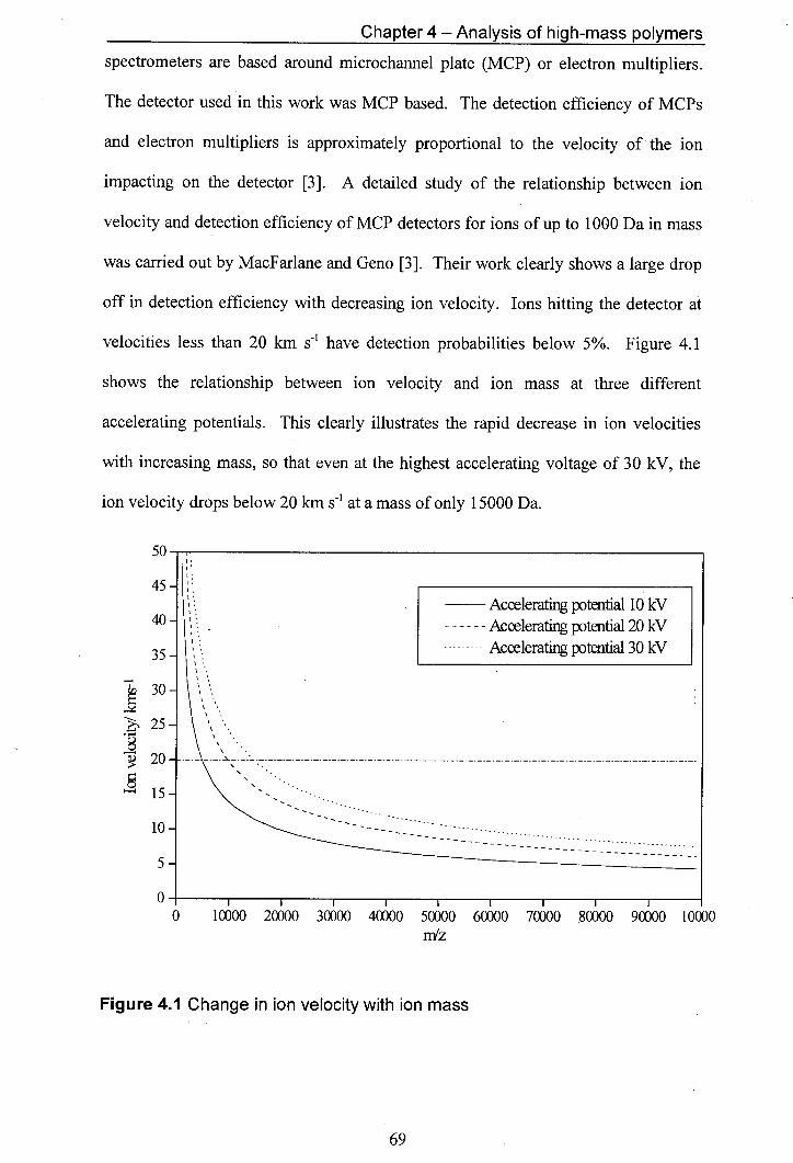
Chapter 4 - Analysis of high-mass polymers
spectrometers are based around microchannel plate (MCP) or electron multipliers.
The detector used in this work was MCP based. The detection efficiency of MCPs
and electron multipliers is approximately proportional to the velocity of the ion
impacting on the detector [3]. A detailed study of the relationship between ion
velocity and detection efficiency of MCP detectors for ions of up to 1000 Da in mass
was carried out by MacFarlane and Geno [3]. Their work clearly shows a large drop
off in detection efficiency with decreasing ion velocity. Ions huffing the detector at
velocities less than 20 km s' have detection probabilities below 5%. Figure 4.1
shows the relationship between ion velocity and ion mass at three different
accelerating potentials. This clearly illustrates the rapid decrease in ion velocities
with increasing mass, so that even at the highest accelerating voltage of 30 kV, the
ion velocity drops below 20 km s' at a mass of only 15000 Da.
50
45 Accelerating potential 10 kV
40
Accelerating potential 20kV
35 Accelerating potential 30 kV
30 25
8 20
15
IS]
5
cii 0 10000 20000 30000 40000 50000 60000 70000 80000 90000 10000
m1z
Figure 4.1 Change in ion velocity with ion mass
M.
Chapter 4 - Analysis of high-mass polymers
In MCP based detectors, like the one used for this research, saturation effects
linked to low mass ions are often observed [4]. In order to detect high-mass ions
high accelerating potentials are used, which leads to very fast low mass ions hitting
the detector before the high-mass ions. The fast low mass ions can produce large
electron currents which often lead to detector saturation. In order to overcome the
saturation problems, a gated deflection plate was installed in the field free drift
region of the mass spectrometer (discussed in detail in section 2.5).
4.3 Sample preparation for high-mass polymers
Sample preparation is of key importance in MALDI. In a recent paper, Li et
al. showed that with the proper choice of matrix and cationising agent, and with
careful sample preparation, it was possible to mass analyse monodisperse polystyrene
samples with average molecular weights up to 1.5 MDa, using a commercial MALDI
mass spectrometer [5]. These impressive results show that, even when using
conventional MALDI equipment, it should be possible to analyse large molecular
weight polymers. However, the analysis of polymers over 100000 Da is rarely
reported in the literature [6,7]. The aim of this work was to extend our working mass
range up to 50000 Da.
In order to test the capability of our mass spectrometer, which was retro-fitted
with a mass gate, polymer calibration standards for GPC columns were analysed.
The polymer standards were purchased from Polymer Laboratories Ltd (Church
70
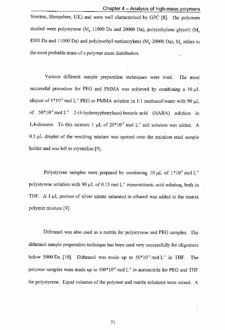
Chapter 4 - Analysis of high-mass polymers
Stretton, Shropshire, UK) and were well characterised by GPC [8]. The polymers
studied were polystyrene (M 11000 Da and 20000 Da), poly(ethylene glycol) (M
8500 Da and 11000 Da) and poly(methyl methacrylate) (M 20000 Da), M refers to
the most probable mass of a polymer mass distribution.
Various different sample preparation techniques were tried. The most
successful procedure for PEG and PMMA was achieved by combining a 10 jiL
aliquot of 1*1 0 mol L' PEG or PMMA solution in 1:1 methanol/water with 90 L
of 50*1 O mol L 1 2-(4-hydroxyphenylazo) benzoic acid (HABA) sokition in
1,4-dioxane. To this mixture 1 pL of 20* 10-3 mol L1 salt solution was added. A
0.5 L droplet of the resulting mixture was spotted onto the stainless steel sample
holder and was left to crystallise [9].
Polystyrene samples were prepared by combining 10 L of 1*1 0 mol L 1
polystyrene solution with 90 jtL of 0.15 mol L' trans-retinoic acid solution, both in
THF. A 1 pL portion of silver nitrate saturated in ethanol was added to the matrix
polymer mixture [9].
Dithranol was also used as a matrix for polystyrene and PEG samples. The
dithranol sample preparation technique has been used very successfully for oligomers
below 5000 Da [10]. Dithranol was made up to 50*10-3 mol U' in THF. The
polymer samples were made up to 100*1 06 mol L' in acetonitrile for PEG and THF
for polystyrene. Equal volumes of the polymer and matrix solutions were mixed. A
71
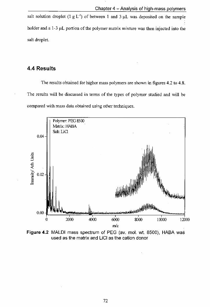
Chapter 4 - Analysis of high-mass polymers
salt solution droplet (1 g L') of between 1 and 3 iL was deposited on the sample
holder and.a 1-3 tL portion of the polymer matrix mixture was then injected into the
salt droplet.
4.4 Results
The results obtained for higher mass polymers are shown in figures 4.2 to 4.8.
The results will be discussed in terms of the types of polymer studied and will be
compared with mass data obtained using other techniques.
0.02
KOI
P 2000 sis:e :{III) 1001 120100 m/z
Figure 4.2 MALDI mass spectrum of PEG (av. mol. wt. 8500), HABA was used as the matrix and LiCI as the cation donor
72
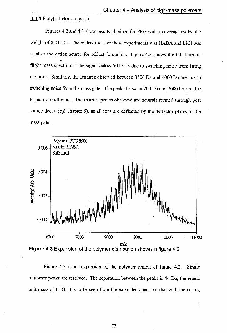
Chapter 4 - Analysis of high-mass polymers
4.4.1 Poly(ethylene glycol)
Figures 4.2 and 4.3 show results obtained for PEG with an average molecular
weight of 8500 Da. The matrix used for these experiments was HABA and LiC1 was
used as the cation source for adduct formation. Figure 4.2 shows the full time-of-
flight mass spectrum. The signal below 50 Da is due to switching noise from firing
the laser. Similarly, the features observed between 3500 Da and 4000 Da are due to
switching noise from the mass gate. The peaks between 200 Da and 2000 Da are due
to matrix multimers. The matrix species observed are neutrals formed through post
source decay (cf chapter 5), as all ions are deflected by the deflector plates of the
mass gate.
Polyner: PEG 8500
[iIiIE1 Ivhtrix: HABA Salt: LiC1
0.004
0.002
ixixs:si
roIl) 'LIIO :iis:s sio ci:oxi:o m/z
Figure 4.3 Expansion of the polymer distribution shown in figure 4.2
Figure 4.3 is an expansion of the polymer region of figure 4.2. Single
oligomer peaks are resolved. The separation between the peaks is 44 Da, the repeat
unit mass of PEG. It can be seen from the expanded spectrum that with increasing
73
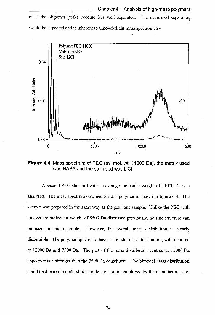
Chapter 4 - Analysis of high-mass polymers
mass the oligomer peaks become less well separated. The decreased separation
would be expected and is inherent to time-of-flight mass spectrometry
'IA
0.02
0 5000 10000 1500 m'z
Figure 4.4 Mass spectrum of PEG (av. mol. wt. 11000 Da), the matrix used was HABA and the salt used was LiCI
A second PEG standard with an average molecular weight of 11000 Da was
analysed. The mass spectrum obtained for this polymer is shown in figure 4.4. The
sample was prepared in the same way as the previous sample. Unlike the PEG with
an average molecular weight of 8500 Da discussed previously, no fine structure can
be seen in this example. However, the overall mass distribution is clearly
discernible. The polymer appears to have a bimodal mass distribution, with maxima
at 12000 Da and 7500 Da. The part of the mass distribution centred at 12000 Da
appears much stronger than the 7500 Da constituent. The bimodal mass distribution
could be due to the method of sample preparation employed by the manufacturer e.g.
74
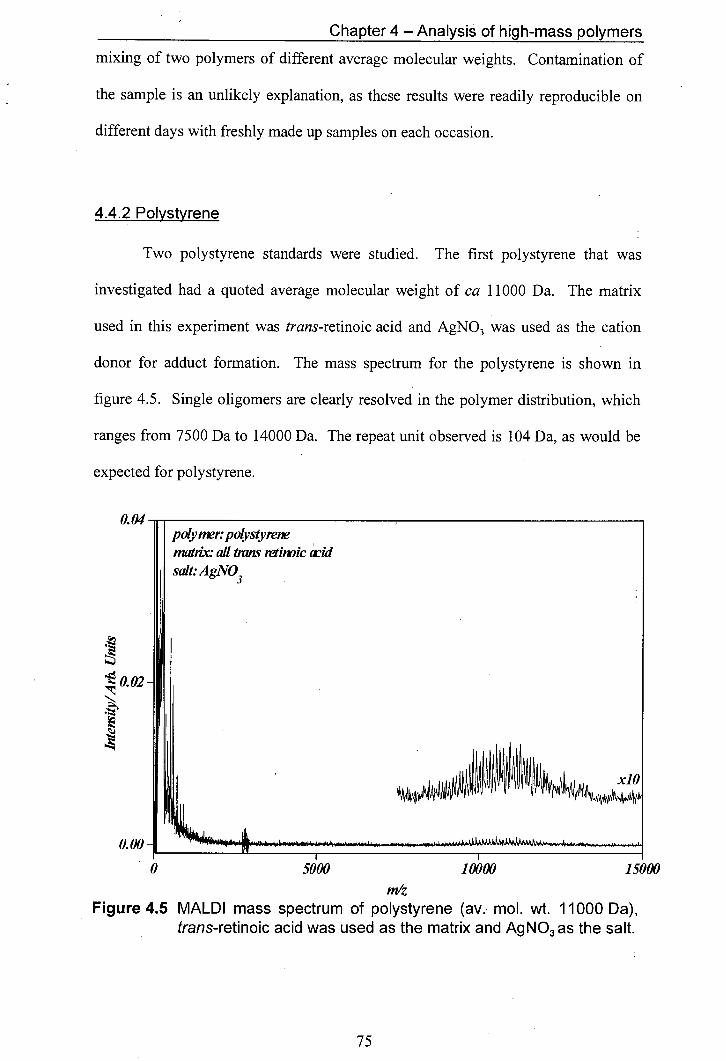
I,,
Chapter 4 - Analysis of high-mass polymers
mixing of two polymers of different average molecular weights. Contamination of
the sample is an unlikely explanation, as these results were readily reproducible on
different days with freshly made up samples on each occasion.
4.4.2 Polystyrene
Two polystyrene standards were studied. The first polystyrene that was
investigated had a quoted average molecular weight of ca 11000 Da. The matrix
used in this experiment was trans-retinoic acid and AgNO3 was used as the cation
donor for adduct formation. The mass spectrum for the polystyrene is shown in
figure 4.5. Single oligomers are clearly resolved in the polymer distribution, which
ranges from 7500 Da to 14000 Da. The repeat unit observed is 104 Da, as would be
expected for polystyrene.
0 5000 10000 15000 mz
Figure 4.5 MALDI mass spectrum of polystyrene (ay.- mol. wt. 11000 Da), trans-retinoic acid was used as the matrix and AgNO3 as the salt.
75
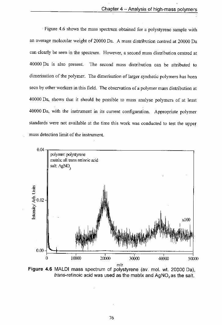
0.02
I
0 10000 20000 30000 40000 50000
Chapter 4 - Analysis of high-mass polymers
Figure 4.6 shows the mass spectrum obtained for a polystyrene sample with
an average molecular weight of 20000 Da. A mass distribution centred at 20000 Da
can clearly be seen in the spectrum. However, a second mass distribution centred at
40000 Da is also present. The second mass distribution can be attributed to
dimerisation of the polymer. The dimerisation of larger synthetic polymers has been
seen by other workers in this field. The observation of a polymer mass distribution at
40000 Da, shows that it should be possible to mass analyse polymers of at least
40000 Da, with the instrument in its current configuration. Appropriate polymer
standards were not available at the time this work was conducted to test the upper
mass detection limit of the instrument.
m/z Figure 4.6 MALDI mass spectrum of polystyrene (av. mol. wt. 20000 Da),
trans-retinoic acid was used as the matrix and AgNO3 as the salt.
,L1
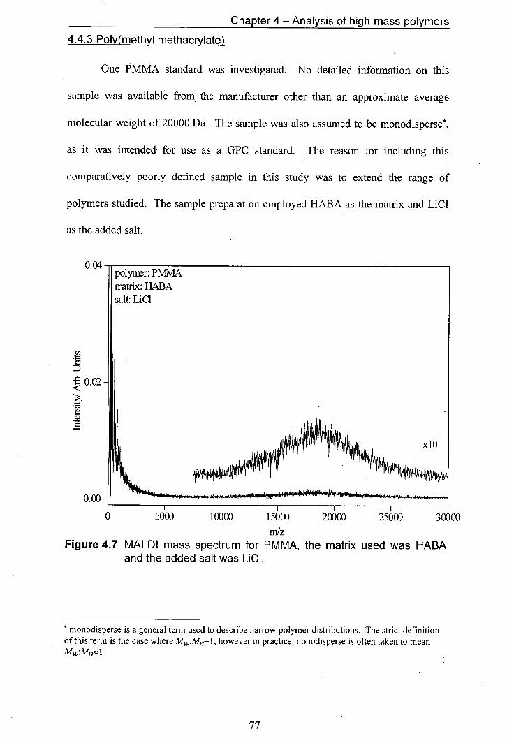
0.02
Chapter 4 - Analysis of high-mass polymers
4.4.3 Poly(methyl methacrylate)
One PMMA standard was investigated. No detailed information on this
sample was available from the manufacturer other than an approximate average
molecular weight of 20000 Da. The sample was also assumed to be monodisperse*,
as it was intended for use as a GPC standard. The reason for including this
comparatively poorly defined sample in this study was to extend the range of
polymers studied. The sample preparation employed HABA as the matrix and LiC1
as the added salt.
0 5000 10000 15000 20000 25000 30000 m/z
Figure 4.7 MALDI mass spectrum for PMMA, the matrix used was HABA and the added salt was LiCI.
monodisperse is a general term used to describe narrow polymer distributions. The strict definition of this term is the case where M:Mn=l, however in practice monodisperse is often taken to mean
Mw: Mn 1
77
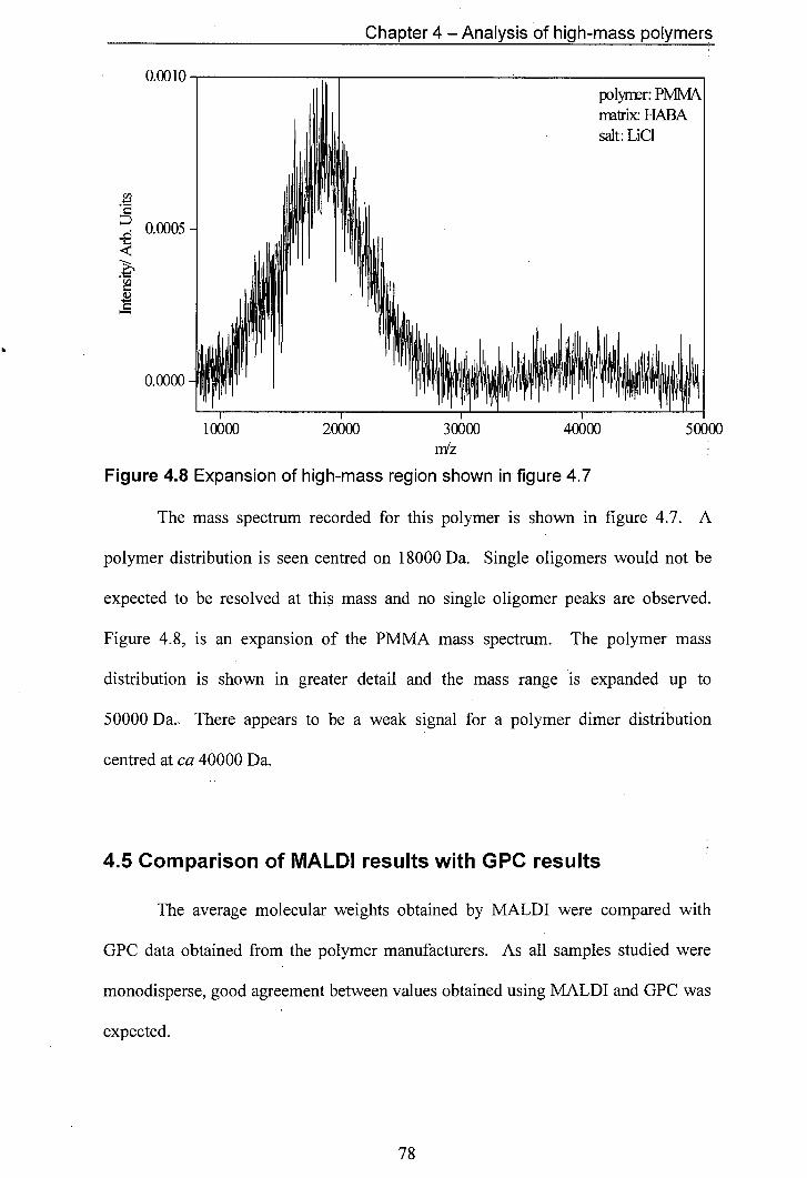
Chapter 4 - Analysis of high-mass polymers
po1ynr: PMIV nntrix: HABA salt: LiC1
0.0005
[11111101
10000 20000 30000 40000 50000 m'z
Figure 4.8 Expansion of high-mass region shown in figure 4.7
The mass spectrum recorded for this polymer is shown in figure 4.7. A
polymer distribution is seen centred on 18000 Da. Single oligomers would not be
expected to be resolved at this mass and no single oligomer peaks are observed.
Figure 4.8, is an expansion of the PMMA mass spectrum. The polymer mass
distribution is shown in greater detail and the mass range is expanded up to
50000 Da. There appears to be a weak signal for a polymer dimer distribution
centred at ca 40000 Da.
4.5 Comparison of MALDI results with GPC results
The average molecular weights obtained by MALDI were compared with
GPC data obtained from the polymer manufacturers. As all samples studied were
monodisperse, good agreement between values obtained using MALDI and GPC was
expected.
78
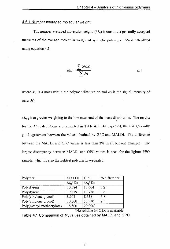
Chapter 4 - Analysis of high-mass polymers
4.5.1 Number averaged molecular weight
The number averaged molecular weight (Mn) is one of the generally accepted
measures of the average molecular weight of synthetic polymers. M is calculated
using equation 4.1
NiMi Mn
I
Ni 4.1
where M is a mass within the polymer distribution and Ni is the signal intensity of
mass M1.
M gives greater weighting to the low mass end of the mass distribution. The results
for the M calculations are presented in Table 4.1. As expected, there is generally
good agreement between the values obtained by GPC and MALDI. The difference
between the MALDI and GPC values is less than 3% in all but one example. The
largest discrepancy between MALDI and GPC values is seen for the lighter PEG
sample, which is also the lightest polymer investigated.
Polymer MALDI GPC % difference M/ Da M/ Da
Polystyrene 10,684 10,664 0.2 Polystyrene 19,879 19,756 0.6 Poly(ethylene glycol) 8,903 8,338 6.8 Poly(ethylene glycol) 10,660 10,930 2.5 Poly(methyl methacrylate) 1 18,500 20,000 -
No reliable UPC Data available Table 4.1 Comparison of M values obtained by MALDI and GPC
79
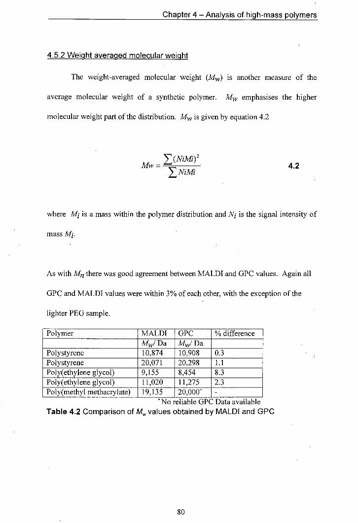
Chapter 4 - Analysis of high-mass polymers
4.5.2 Weight averaged molecular weight
The weight-averaged molecular weight (Mw) is another measure of the
average molecular weight of a synthetic polymer. Mw emphasises the higher
molecular weight part of the distribution. Mw is given by equation 4.2
MW
I (NiMi)2 4.2
NiMi
where M1 is a mass within the polymer distribution and Ni is the signal intensity of
mass M1.
As with M there was good agreement between MALDI and GPC values. Again all
GPC and MALDI values were within 3% of each other, with the exception of the
lighter PEG sample.
Polymer MALDI GPC % difference Mw/ Da MwIDa
Polystyrene 10,874 10,908 0.3 Polystyrene 20,071 20,298 1.1 Poly(ethylene glycol) 9,155 8,454 8.3 Poly(ethylene glycol) 11,020 11,275 2.3 Poly(methyl methacrylate) 19,135 20,000* -
No reliable GPC Data available Table 4.2 Comparison of M values obtained by MALDI and GPC
HE
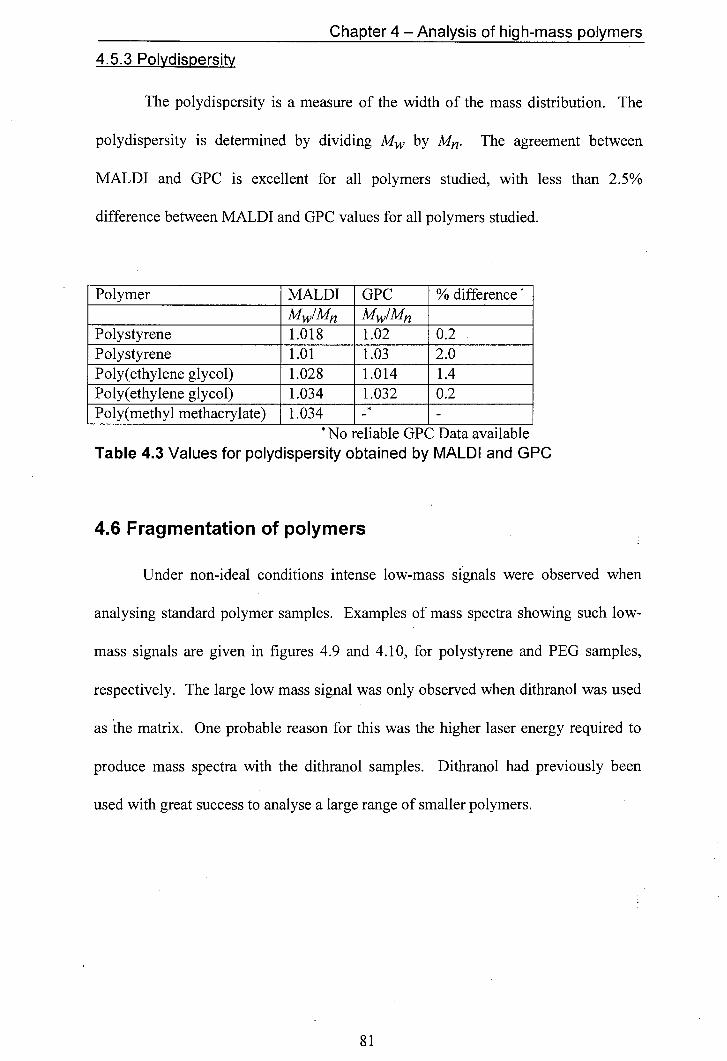
Chapter 4 - Analysis of high-mass polymers
4.5.3 Polydispersity
The polydispersity is a measure of the width of the mass distribution. The
polydispersity is determined by dividing Mw by M. The agreement between
MALDI and GPC is excellent for all polymers studied, with less than 2.5%
difference between MALDI and GPC values for all polymers studied.
Polymer MALDI GPC % difference
M/M M/M Polystyrene 1.018 1.02 0.2 Polystyrene 1.01 1.03 2.0 Poly(ethylene glycol) 1.028 1.014 1.4 Poly(ethylene glycol) 1.034 1.032 0.2 Poly(methyl methacrylate) 1.034 -
* No reliable GPC Data available Table 4.3 Values for polydispersity obtained by MALDI and GPC
46 Fragmentation of polymers
Under non-ideal conditions intense low-mass signals were observed when
analysing standard polymer samples. Examples of mass spectra showing such low-
mass signals are given in figures 4.9 and 4.10, for polystyrene and PEG samples,
respectively. The large low mass signal was only observed when dithranol was used
as the matrix. One probable reason for this was the higher laser energy required to
produce mass spectra with the dithranol samples. Dithranol had previously been
used with great success to analyse a large range of smaller polymers.
81

Chapter 4 - Analysis of high-mass polymers
Polymer: polystyrene 1 Matrix: dithranol Salt: AgCF3CO2
0.002
4000 6000 8000 10000 12000 14000 16000
m/z
Figure 4.9 Mass spectrum of polystyrene 12860 with, an unusual sloping
feature (mlz = 4000- 10000). The matrix used was dithranol and
the salt used was AgCF3CO2
Figure 4.9 shows a mass spectrum of polystyrene. A sloping feature
extending from 4000 Da to 10000 Da can be seen as well as the polymer distribution,
extending from 10000 Da to 16000 Da. The mass gate deflected all ions of mass
lower than 4000 Da, which led to the cut-off at 4000 Da. The sloping feature
exhibits no discernible fine structure. The large signal around 7000 Da is due to
switching noise from the mass gate.
82

Chapter 4 - Analysis of high-mass polymers
0.016
Polymer: PEG 11840 Matrix: dithranol
0.014
Salt: LiC1
0.012
0.010
0.008
0.006
,xsI,p.1
[11111)1
0 2000 4000 6000 8000 10000 12000 14000 16000
m/z
Figure 4.10 Mass spectrum for PEG exhibiting a sloping background
The spectrum in figure 4.10 is dominated by a sloping background extending
from 2000 Da upward in mass. The cut-off at 2000 Da is due to the mass gate, which
deflected all ions below 2000 Da in mass. Superimposed on the sloping background
is the polymer distribution, extending from 10000 Da to 14000 Da. An expansion of
the mass region 2400 Da to 3050 Da reveals well resolved peaks within the sloping
part of the mass spectrum (see figure 4.11). Three series of peaks, two strong series
and one series of peaks of lower intensity are observed. The separation between
peaks in each series is 44 Da, the repeat unit of PEG. These peaks were most
probably due to fragmentation products of PEG oligomers. The fragmentation
behaviour of polyglycols is well documented and it is thus possible to confirm that
the peaks are due to fragment ions [11].
83
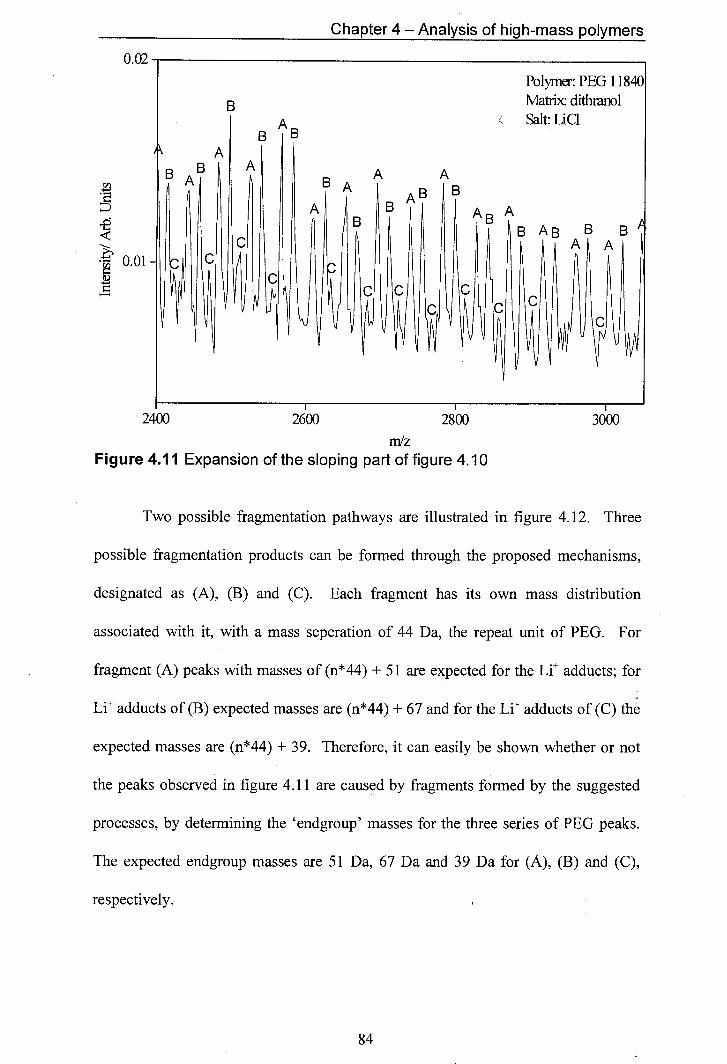
Chapter 4 - Analysis of high-mass polymers
n m Polymer: PEG 11840
B Matrix: dithranol Salt:LiC1 B AB
A B Bt A
A BA A A
A B A B kA WBB
C ki jIB]
C
I I
S's Is'
m/z Figure 4.11 Expansion of the sloping part of figure 4.10
Two possible fragmentation pathways are illustrated in figure 4.12. Three
possible fragmentation products can be formed through the proposed mechanisms,
designated as (A), (B) and (C). Each fragment has its own mass distribution
associated with it, with a mass seperation of 44 Da, the repeat unit of PEG. For
fragment (A) peaks with masses of (n*44) + 51 are expected for the Li adducts; for
Li adducts of (B) expected masses are (n*44) + 67 and for the Li adducts of (C) the
expected masses are (n*44) + 39. Therefore, it can easily be shown whether or not
the peaks observed in figure 4.11 are caused by fragments formed by the suggested
processes, by determining the 'endgroup' masses for the three series of PEG peaks.
The expected endgroup masses are 51 Da, 67 Da and 39 Da for (A), (B) and (C),
respectively.
0.01
84
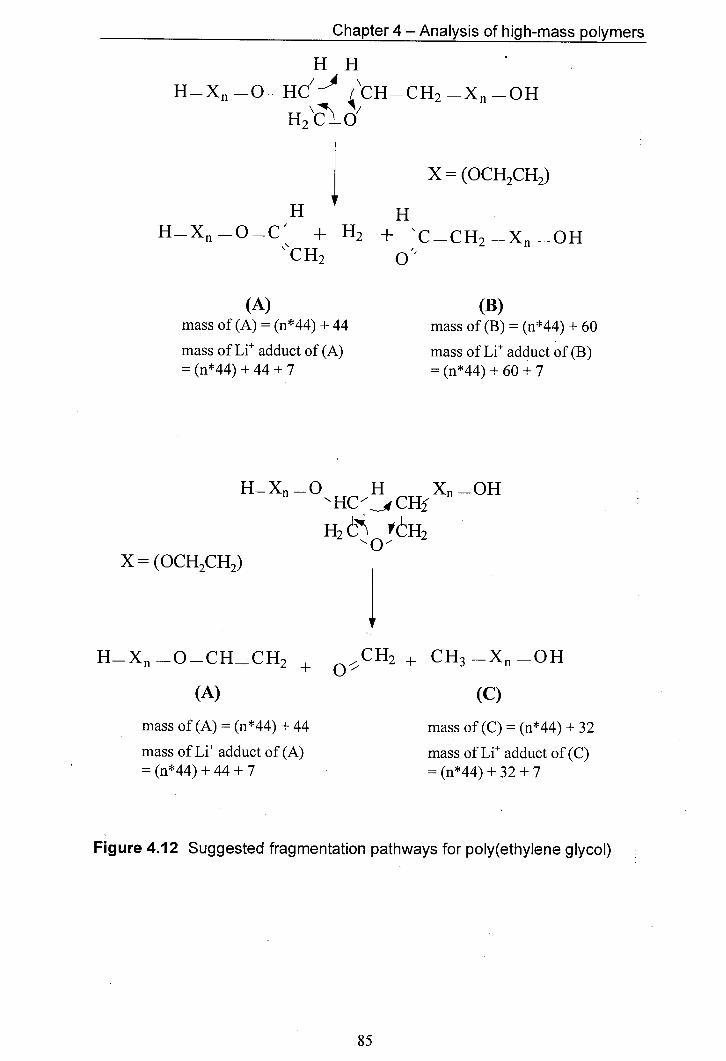
Chapter 4 - Analysis of high-mass polymers
H—X —O—HC 4CH_CH2 —X —OH
H2 C 0'
X = (OCH2CH2)
H IF
H_X_O_C' + H2 CH2
(A) mass of (A) = (n*44) + 44
mass of Li adduct of (A) = (n*44) + 44 + 7
H + 'C—CH2 _X—OH
0"
(B) mass of (B) = (n*44) + 60
mass of Li adduct of (B) = (n*44) + 60 + 7
H_X_O H Xe _OH HC- CHI
H2 H2
X = (OCH2CH2)
H_X_O_CHCH2 + 0 CH2 + CH3 —X---OH
(A)
(C)
mass of (A) = (n*44) +44 mass of (C) = (n*44) + 32
mass of Li adduct of (A) mass of Li adduct of (C) = (n*44) + 44 + 7 n*44)+32+7
Figure 4.12 Suggested fragmentation pathways for poly(ethylene glycol)
85
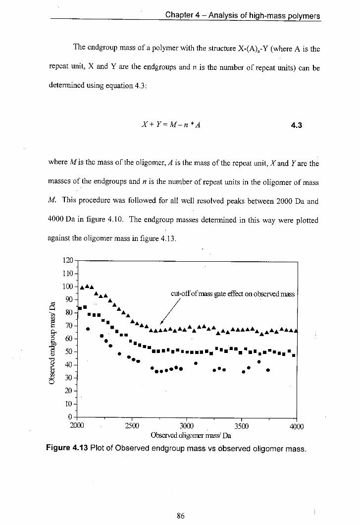
Chapter 4 - Analysis of high-mass polymers
The endgroup mass of a polymer with the structure X-(A)-Y (where A is the
repeat unit, X and Y are the endgroups and n is the number of repeat units) can be
determined using equation 4.3:
X+ YM—n *A
4.3
where Mis the mass of the oligomer, A is the mass of the repeat unit, X and V are the
masses of the endgroups and n is the number of repeat units in the oligomer of mass
M. This procedure was followed for all well resolved peaks between 2000 Da and
4000 Da in figure 4.10. The endgroup masses determined in this way were plotted
against the oligomer mass in figure 4.13.
120-
110-
100- AAA cut-off of mass gate effect on observed mass
90- A
80 1
70- • . AAAA A AA AAA 60
S
50 .I
- ••uUU......IUIIIIUl OEM ulU.u.. IuU _ .I.Uui
- .S.
. S 413- • • 30
20-
10-
0- I I
2000 2500 3000 3500 4000 Observed oligon-er mass/ Da
Figure 4.13 Plot of Observed endgroup mass vs observed oligomer mass.
86
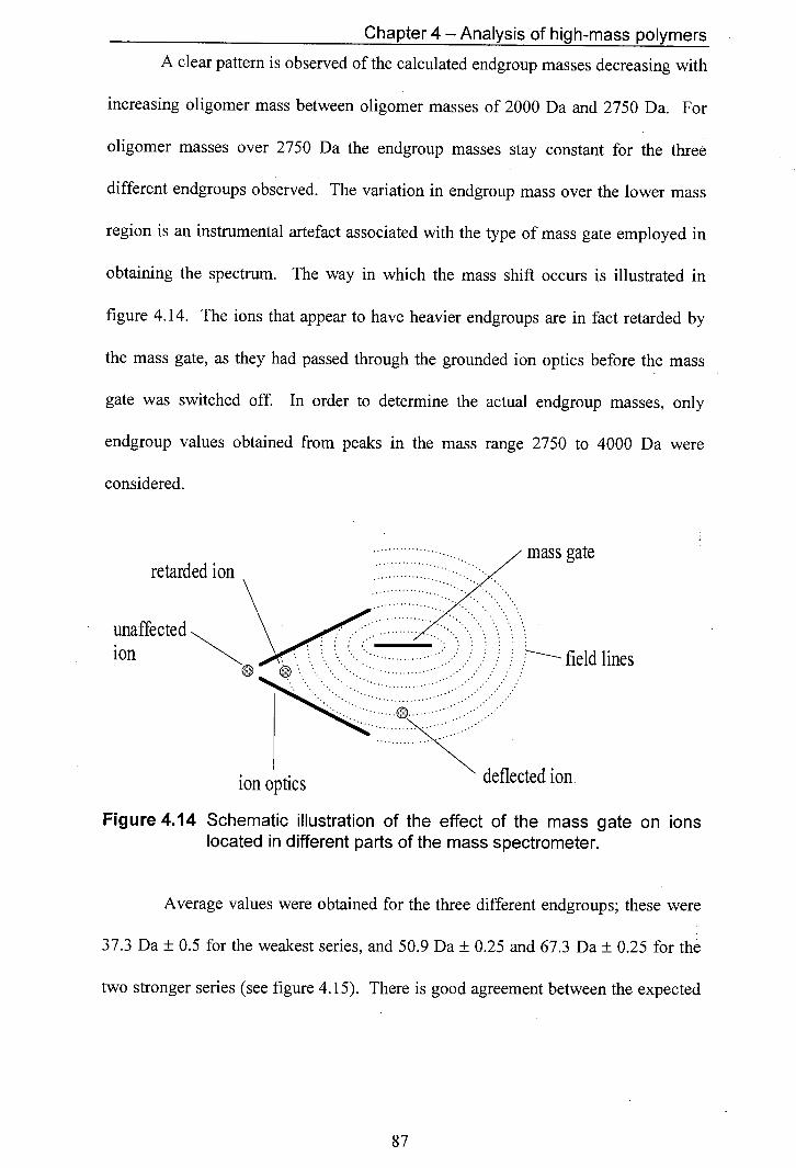
lull
ion optics
Chapter 4 - Analysis of high-mass polymers
A clear pattern is observed of the calculated endgroup masses decreasing with
increasing oligomer mass between oligomer masses of 2000 Da and 2750 Da. For
oligomer masses over 2750 Da the endgroup masses stay constant for the three
different endgroups observed. The variation in endgroup mass over the lower mass
region is an instrumental artefact associated with the type of mass gate employed in
obtaining the spectrum. The way in which the mass shift occurs is illustrated in
figure 4.14. The ions that appear to have heavier endgroups are in fact retarded by
the mass gate, as they had passed through the grounded ion optics before the mass
gate was switched off. In order to determine the actual endgroup masses, only
endgroup values obtained from peaks in the mass range 2750 to 4000 Da were
considered.
Figure 4.14 Schematic illustration of the effect of the mass gate on ions located in different parts of the mass spectrometer.
Average values were obtained for the three different endgroups; these were
37.3 Da ± 0.5 for the weakest series, and 50.9 Da ± 0.25 and 67.3 Da ± 0.25 for the
two stronger series (see figure 4.15). There is good agreement between the expected
87
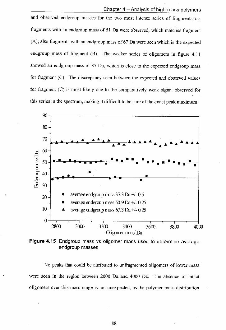
Chapter 4 - Analysis of high-mass polymers
and observed endgroup masses for the two most intense series of fragments i.e.
fragments with an endgroup mass of 51 Da were observed, which matches fragment
(A); also fragments with an endgroup mass of 67 Da were seen which is the expected
endgroup mass of fragment (B). The weaker series of oligomers in figure 4.11
showed an endgroup mass of 37 Da, which is close to the expected endgroup mass
for fragment (C). The discrepancy seen between the expected and observed values
for fragment (C) is most likely due to the comparatively weak signal observed for
this series in the spectrum, making it difficult to be sure of the exact peak maximum.
-MI
70-
I
30
20-
10-
AAAAAA AAAA A A AA A A A A * AAA
U • • •l • •U • • •
average endgroup mass 37.3 Da +1- 0.5
average endgroup mass 50.9 Da +/- 0.25 A average endgroup mass 67.3 Da +1- 0.25
2800 3000 3200 3400 3600 3800 4000 aiOnr miss! Da
Figure 4.15 Endgroup mass vs oligomer mass used to determine average endgroup masses
No peaks that could be attributed to unfragmented oligomers of lower mass
were seen in the region between 2000 Da and 4000 Da. The absence of intact
oligomers over this mass range is not unexpected, as the polymer mass distribution
88
Chapter 4 - Analysis of high-mass polymers
has been shown to be very narrow and confined to a range extending from 10000 Da
to 15000 Da (see figure 4.4). Clearly the fragment ions must not be included, when
the average molecular weights are calculated. In the example given here, it was easy
to distinguish between fragments and molecular ions, as the fragments were well
resolved; however, it is obvious that fragmentation could cause a significant
distortion of average molecular weights. Inclusion of fragments in the molecular
weight distribution is most likely to occur, when fragments and molecular ions are
not readily distinguishable, e.g when the resolution does not allow for the
identification of single peaks or if there is a strong overlap between fragments and
molecular ions. It is therefore very important for accurate average molecular weight
determinations that fragmentation be minimised. Fragmentation can be minimised
by good sample preparation and judicious use of laser power.
4.7 Conclusions
This chapter shows that with a few instrumental modifications and careful
sample preparation, it is possible to characterise polymers with average molecular
weights in excess of 5000 Da. The highest mass polymer observed in these
experiments had an average molecular weight of around 40000 Da, i.e. the dimer
ions of polystyrene with an average monomer molecular weight of 20000 Da. The
results obtained for a range of polymers by MALDI were compared with the
manufacturer's values obtained using GPC. Good agreement was found between the
MALDI and the GPC data. Fragmentation was observed when sample preparation
was not carried out well. Fragmentation must be carefully controlled and minimised
in order to obtain reliable molecular weight data.
89

Chapter 4 - Analysis of high-mass polymers
4.8 References
D. C. Imrie, J. M. Pentney and J. S. Cottrell, Rapid Commun. Mass Spectrom., 9, 1293-1296 (1995) U. Bahr, U. Rohling, C. Lautz, K. Strupat, M. Schurenberg and F. Hillenkamp, Int. I Mass Spectrom. Ion Proc., 153, 9-21 (1996) P. W. Geno and R. D. MacFarlane, mt. I Mass Spectrom. Ion Proc., 92, 195-210 (1989) A. Westman, G. Brinkmalm and D. F. Barofsky, mt. I Mass Spectrom. Ion Proc., 169/170, 79-87 (1997) D. C. Schriemer and L. Li, Anal. Chem., 68, 2721-2725 (1996) P. 0. Danis and D. E. Karr, Org. Mass Spectrom., 28, 923-925 (1993) P. 0. Danis, D. E. Karr, F. Mayer, A. Holle and C. H. Watson, Org. Mass Spectrom., 27, 843-846 (1992) Calibration notices from Polymer Laboratories Ltd (Church Stretton, Shropshire, UK) R. M. Whittal, D. C. Scbriemer and L. Li, Anal. Chem., 69, 2734-2741 (1997) Ian A. Mowat, PhD Thesis, The University of Edinburgh (1995) L. R. Hittle, D. E. Altiand, A. Proctor and D. M. Hercules, Anal. Chem., 66 2302-2305 (1994)
Chapter 5 - Metal ion detachment studies
Chapter 5— Metal ion detachment studies
5.1 Introduction
The analyte ion species detected in MALDI experiments is usually a neutral-
ion complex, commonly referred to as an ion adduct [1]. For peptides and proteins
proton adducts are most often seen although alkali metal adducts are also known to
form [2]. Synthetic polymers do not readily form adducts with protons but they do
form adducts with metal ions [3,4]. The specific metal ion best suited to adduct
formation is polymer dependent, although often a range of different metal ions can be
used. Several studies have been conducted into metal ion polymer adduct formation
[3,5,6]. Metal cations have been shown to attach readily to polystyrene,
poly(ethylene glycol) and polybutadiene in JR laser-desorption/time-of-flight
experiments [7,8]. Studies of metal ion attachment to polymers under typical
MALDI conditions, using salts containing metals of different oxidation states, have
shown that only singly charged metal polymer adducts are formed, regardless of the
oxidation state of the metal ion in the salt [3,6]. In a recent paper Scrivens et al.
investigated the collision-induced dissociation (CID) of the alkali metal adducts of
poly(methyl methacrylate) (PMMA) oligomers [9]. Different fragmentation patterns
were found with different alkali metal ion adducts. The fragmentation was also
91
Chapter 5 - Metal ion detachment studies
shown to vary with oligomer size. As well as fragment ions, a large signal from the
bare alkali ions was also observed indicating the loss of the metal ion from the
adduct. The alkali metal ion yield was particularly noticeable for Rb and Cs
adducts.
The work presented here focuses on the spontaneous post source decay (PSD)
of polymer metal ion adducts under standard MALDI conditions. The effect of PSD
on the average molecular weight distribution of an oligomeric system was
investigated.
52 Experimental
For the experiments presented here, the mass spectrometer was operated in
two different modes; these were the linear and reflectron modes. In the linear mode,
the reflectron was switched off (i.e. connected to ground). In this mode of operation,
all species that were transmitted into the drift region of the mass spectrometer were
detected on the in-line micro channel plate (MCP) detector as illustrated in figure 5.1.
The other mode of operation was termed the reflectron mode. In the reflectron mode
the reflectron would be switched on. The reflectron is a retarding field produced by a
series of lens elements, which are coupled together by a resistor chain, giving rise to
a graded field. The front grid of the reflectron is at ground potential and the rear grid
is at a high potential, the field strength increasing along the length of the reflectron.
The effect that switching on the reflectron has is to retard any charged species that
enter it. If the potential on the final element of the reflectron is higher than the
92
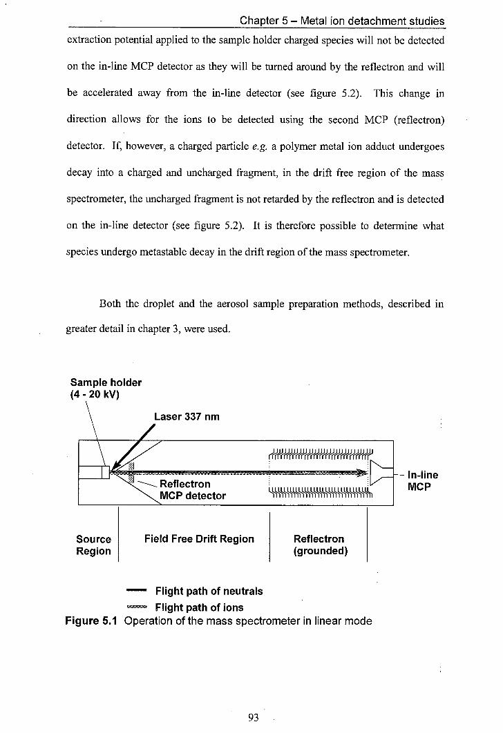
Chapter 5 - Metal ion detachment studies
extraction potential applied to the sample holder charged species will not be detected
on the in-line MCP detector as they will be turned around by the reflectron and will
be accelerated away from the in-line detector (see figure 5.2). This change in
direction allows for the ions to be detected using the second MCP (reflectron)
detector. If, however, a charged particle e.g. a polymer metal ion adduct undergoes
decay into a charged and uncharged fragment, in the drift free region of the mass
spectrometer, the uncharged fragment is not retarded by the reflectron and is detected
on the in-line detector (see figure 5.2). It is therefore possible to determine what
species undergo metastable decay in the drift region of the mass spectrometer.
Both the droplet and the aerosol sample preparation methods, described in
greater detail in chapter 3, were used.
Sample holder (4 - 20 kV)
Laser 337 nm
Reflectron MCP detector
Source Field Free Drift Region Reflectron Region (grounded)
- Flight path of neutrals
Flight path of ions Figure 5.1 Operation of the mass spectrometer in linear mode
In-line MCP
93
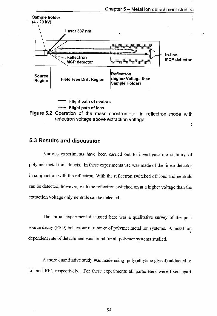
Chapter 5 - Metal ion detachment studies
Sample holder (4-20kV)
Laser 337 nm
----... Reflectron 'N. MCP detector
In-line MCP detector
Source Region I
Field Free Drift Region Reflectron (higher Voltage Sample Holder)
- Flight path of neutrals
Flight path of ions Figure 5.2 Operation of the mass spectrometer in reflection mode with
reflectron voltage above extraction voltage.
5.3 Results and discussion
Various experiments have been carried out to investigate the stability of
polymer metal ion adducts. In these experiments use was made of the linear detector
in conjunction with the reflectron. With the reflectron switched off ions and neutrals
can be detected; however, with the reflectron switched on at a higher voltage than the
extraction voltage only neutrals can be detected.
The initial experiment discussed here was a qualitative survey of the post
source decay (P SD) behaviour of a range of polymer metal ion systems. A metal ion
dependent rate of detachment was found for all polymer systems studied.
A more quantitative study was made using poly(ethylene glycol) adducted to
Li and Rb, respectively. For these experiments all parameters were fixed apart
94
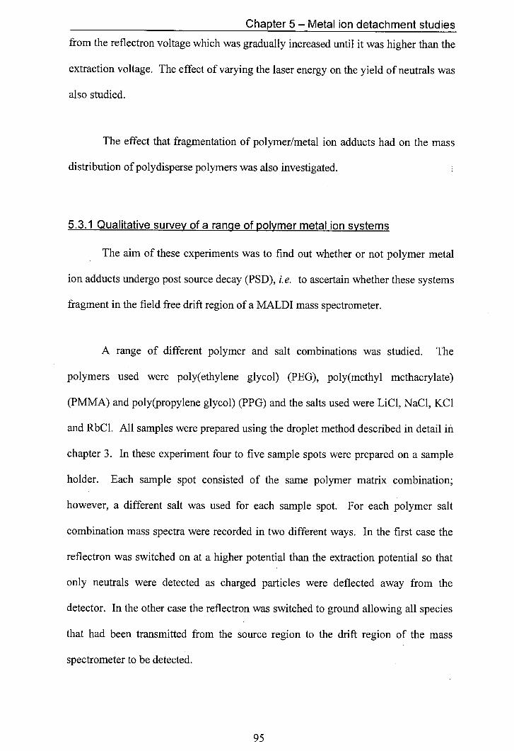
Chapter 5 - Metal ion detachment studies
from the reflectron voltage which was gradually increased until it was higher than the
extraction voltage. The effect of varying the laser energy on the yield of neutrals was
also studied.
The effect that fragmentation of polymer/metal ion adducts had on the mass
distribution of polydisperse polymers was also investigated,
5.3.1 Qualitative survey of a range of polymer metal ion systems
The aim of these experiments was to find out whether or not polymer metal
ion adducts undergo post source decay (PSD), i.e. to ascertain whether these systems
fragment in the field free drift region of a MALDI mass spectrometer.
A range of different polymer and salt combinations was studied. The
polymers used were poly(ethylene glycol) (PEG), poly(methyl methacrylate)
(PMMA) and poly(ropylene glycol) (PPG) and the salts used were LiC1, NaCl, KC1
and RbCl. All samples were prepared using the droplet method described in detail in
chapter 3. In these experiment four to five sample spots were prepared on a sample
holder. Each sample spot consisted of the same polymer matrix combination;
however, a different salt was used for each sample spot. For each polymer salt
combination mass spectra were recorded in two different ways. In the first case the
reflectron was switched on at a higher potential than the extraction potential so that
only neutrals were detected as charged particles were deflected away from the
detector. In the other case the reflectron was switched to ground allowing all species
that had been transmitted from the source region to the drift region of the mass
spectrometer to be detected.
95
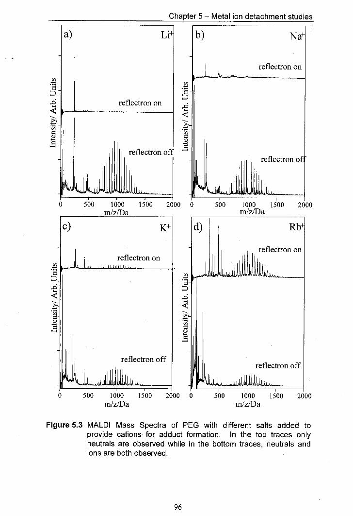
I
Chapter 5 - Metal ion detachment studies
0 500 1000 1500 2000 0 500 1000 1500 2000 mlz/Da mIzIDa
d)
reflectron on
reflectron off I
0 500 1000 1500 2000 0 500 1000 1500 2000 mlz/Da m!z/Da
Figure 5.3 MALDI Mass Spectra of PEG with different salts added to provide cations- for adduct formation. In the top traces only neutrals are observed while in the bottom traces, neutrals and ions are both observed.
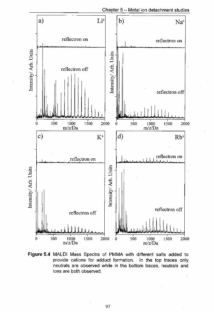
Chapter 5 - Metal ion detachment studies
a) Li
reflectron on
- reflectron off
0 500 1000 1500 2000 0 500 1000 1500 2000 mlz/Da m!z/Da
-4
I
d) Rb
reflectron on
4-1
reflectron off
0 500 1000 1500 2000 0 500 1000 1500 2000 m/z/Da mlz/Da
Figure 5.4 MALDI Mass Spectra of PMMA with different salts added to provide cations for adduct formation. In the top traces only neutrals are observed while in the bottom traces, neutrals and ions are both observed.
97
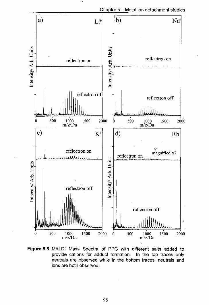
Chapter 5 - Metal ion detachment studies
cI
I 0 500 1000 1500 2000 0
500 1000 1500 2000
m!z/Da m!z/Da
d) Rb
reflectron on magnified x2
reflectron off
L1LLIjjjjJJ.A.A
0 500 1000 1500 2000 0 500 1000 1500 2000 mlz/Da mlz/Da
Figure 5.5 MALDI Mass Spectra of PPG with different salts added to provide cations for adduct formation. In the top traces only neutrals are observed while in the bottom traces, neutrals and ions are both observed.
98
Chapter 5 - Metal ion detachment studies
All other experimental parameters, such as the extraction voltage, the gain on the
detector and the laser energy, were kept constant.
The results of these experiments showed the same trend for all systems
studied. It was found that the larger the metal ion attached to the polymer, the more
likely the polymer metal ion adduct was to undergo PSD. These trends will be
illustrated here for PEG, PPG and PMMA with Li, Na, K and Rb attachment; the
same phenomena were, however, also observed for higher molecular weight samples.
The results obtained for the PEG system are shown in figures 5.3 a-d. The mass
spectrum for PEG with LiC1 with the reflectron switched to ground is shown in the
part spectrum of figure 5.3 a. A polymer distribution can clearly be seen centred on
1000 Da. The separation between oligomer peaks is 44 Da the PEG repeat unit mass.
The peaks in the region between 0 and 500 Da are due to metal ions (lithium at 7 Da,
sodium at 23 Da and potassium at 39 Da) and to dithranol species e.g. the proton
adduct of the matrix at 227 Da and at 233 Da, the lithium adduct of the matrix a
well as some higher mass peaks caused by protonated and lithiated matrix clusters. It
is not clear what the unresolved features underlying the mass spectrum at 500 Da,
750 Da and 1000 Da are; however, they could be due to dithranol clusters. The top
mass spectrum in figure 5.3 a was recorded for the lithium PEG system while all ions
were deflected away from the detector using the reflectron. As can clearly be seen
very few peaks are present in this mass spectrum and notably no peaks are associated
with polymer lithium adducts. The most intense peak in this mass spectrum is due to
neutrals formed from protonated dithranol. The absence of any polymer-related
peaks shows that PEG lithium adducts do not decay under the experimental
Chapter 5 - Metal ion detachment studies
conditions. It should also be stressed that no metal ions were detected with the
reflectron on, confirming that no charged species were detected with the reflectron at
a higher potential than the extraction voltage.
The mass spectra for the NaCl PEG combination (figure 5.3 b) show broadly
similar features to the equivalent LiCl PEG mass spectra. The most obvious
difference between the mass spectrum for NaCl and PEG with the reflectron off and
the corresponding LiC1 and PEG mass spectrum is that two overlapping polymer
mass distributions are seen in the NaCl case. The major polymer distribution is due
to sodiated PEG oligomers whereas the lower intensity polymer distribution, which
is offset by 16 Da from the main polymer distribution, can be ascribed to potassiated
PEG. Potassium is often found as a contaminant in MALDI mass spectrometry. The
top mass spectrum of figure 5.3 b shows no peaks due to polymer related species.
The most intense peak is due to neutrals associated with sodiated matrix.
Figure 5.3 c shows the mass spectra for the PEG KC1 combination. The
lower mass spectrum was recorded with the reflectron off. It shows both sodiated
and potassiated PEG oligomers. The less intense polymer distribution being due to
sodiated PEG oligomers. The top mass spectrum of figure 5.3 c was recorded with
the reflectron on. This mass spectrum is very different from the comparable mass
spectra for the lithium and sodium PEG cases as signals corresponding to neutral
dissociation products of potassium PEG adducts were observed. It should be noted
that only neutrals formed from potassiated PEG oligomers were seen in this mass
spectrum. Other neutrals detected were matrix species.
100
Chapter 5 - Metal ion detachment studies
The mass spectra for the RbC1 PEG system (figure 5.3 d) show that the Rb
adducts of PEG also undergo PSD. Here the signal intensity of the polymer peaks in
the upper mass spectrum, i.e. the mass spectrum showing only neutral species, is
higher than for the lower mass spectrum in which both charged and uncharged
particles were detected. As signal intensity can often be used as an approximate
measure of the number of particles detected, peaks in mass spectra recorded with the
reflectron on would be expected to be less intense than the equivalent peaks in mass
spectra recorded with the reflectron off. This is clearly not the case for the polymer
peaks in figure 5.3 d. The main reason for this is believed to be detector saturation
occurring in the reflectron-off mode due to the large number of low mass ions
impacting on the detector which are largely deflected for reflectron-on experiments
(see chapter 2 for detailed discussion) [10].
There is a clear trend for the fragmentation of the alkali metal adducts of
PEG. The amount of fragmentation observed increases with the size of the alkali
metal ion. Whereas lithiated and sodiated PEG does not undergo PSD, both
potassiated and rubidiated PEG do.
Similar experiments to those described for PEG were also carried out for
PMMA and PPG (figures 5.4 and 5.5). The same trend was observed, i.e. the adducts
of the heavier alkali metals, rubidium for PMMA and potassium and rubidium for
PPG, underwent PSD whereas dissociation products were not detected for the
adducts of the lighter alkali metals.
101
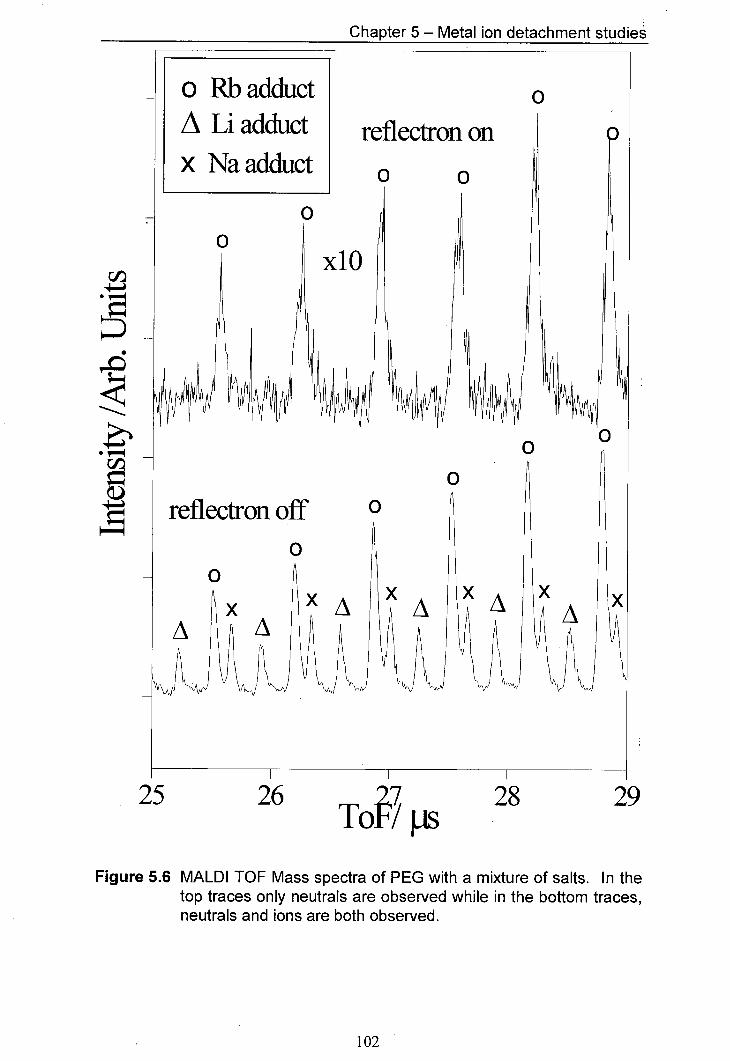
Chapter 5 - Metal ion detachment studies'
o Rh adduct A Li adduct x Na adduct
reflectron on
0 0
xlO
ME
reflectron off 0
0
X L
25 26 To? 28 29
Figure 5.6 MALDI TOF Mass spectra of PEG with a mixture of salts. In the top traces only neutrals are observed while in the bottom traces, neutrals and ions are both observed.
102

Chapter 5 - Metal ion detachment studies
A further experiment was carried out to confirm that the neutral formation
observed in the previous experiments was metal ion dependent. A mixture of LiC1
and RbC1 was used in the sample preparation rather than a single salt to show that
under identical conditions Rb adducts dissociate whereas Li adducts do not. The
sample prepared for this experiment used PEG and dithranol for the polymer and
matrix and a mixture of LiC1 and RbC1 as the salt. The RbCl concentration (0.0165
M in deionised water) was 30 times larger than the LiC1 concentration (0.5x10 3 M in
deionised water). At a RbC1 to LiC1 ratio of 30:1 Rb and Li adducts of PEG are
both observed, whereas, at a 1:1 ratio, no Rb adduct is observed. The sample was
prepared using the aerosol method.
The results for the mixed salts experiment are presented in figure 5.6. When
the reflectron is on and only neutrals are detected, only peaks associated with the Rb
adduct of PEG was observed. In the reflectron-off mode, Li and Rb adducts were
detected, as well as some Na adducts. This experiment shows that, under identical
conditions, neutral decay products of the Rb adducts of PEG were detected whereas
no such species were detected for Li and Na adducts. These findings indicate that
rubidium-containing PEG adducts undergo PSD under typical MALDI conditions
and that lithium and sodium adducts of PEG are not subject to PSD.
This initial survey has shown that the tendency for polymer metal adduct ions
to dissociate post-source is metal ion dependent. Lithium and sodium-containing
polymer adducts do not dissociate post source at a detectable level under typical
MALDI conditions. However, a significant fraction of potassium and rubidium
103
Chapter 5 - Metal ion detachment studies
adducts of the polymers studied fragmented in the drift free region of the mass
spectrometer.
5.3.2 Post acceleration
It was noted during the initial experiments that neutral fragments had a longer
flight time than their charged parent species. The delay seen was ca 50 ns over a
flight time of 30 j.xs, the typical flight time of an ion with a mass of 1000 Da at an
accelerating voltage of 4 kV (see figure 5.7 a). There are several possible reasons for
retardation of neutral fragments. It is conceivable that most of the fragmentation of
the adducts occurs in the source region of the mass spectrometer, when the adduct is
still being accelerated by the extraction potential. In-source decay would lead to a
time delay, as the adduct would not have reached its final velocity at the time of
fragmentation and hence the neutral fragment would be moving at a velocity lower
than that of the intact adduct. Extensive in-source decay, however, would not just
bring about longer average flight times but also considerable peak broadening would
be seen for the decay product peaks, as the decay would occur at different stages of
the acceleration process. Such peak broadening would be so extensive that detection
of neutrals produced in-source would be unlikely. Some peak broadening was seen
(see figure 5.7 a) but it is not extensive.
Another possible reason for the delay of the neutrals could be deceleration of
ions, by the reflectron prior to decay; however, this process again would have been
accompanied by a large amount of peak broadening which was not observed.
104
Chapter 5 - Metal ion detachment studies
The most probable reason for the longer flight times of neutrals compared
with those of ions is the post acceleration potential applied to the detector. In order
to increase the detection efficiency of the MCP detector, its front face was
maintained at a negative potential of -2 kV, which accelerates positive ions into the
detector and hence increases their kinetic energy. The post acceleration potential
also leads to a decrease of the flight time of positively charged species. Neutral
species are not affected by the post acceleration potential and therefore exhibit longer
flight times than their parent ions.
A simple experiment was carried out to show whether or not the delay observed was
due to the post acceleration or not. For this experiment a sample of RbC1 with PEG
was made up using the aerosol technique. The detector was set up so that the front
face of the detector was at ground potential. Mass spectra were recorded as before,
with the reflectron on and with the reflectron off. The same experiment was carried
out with the detector set up conventionally, i.e. with the -2 kV post acceleration
potential. The results are presented in figure 5.7 a for the conventional set-up and
figure 5.7 b for the non-post-accelerated set-up. As can be seen from the results, the
neutral peaks, i.e. the mass spectrum recorded with the reflectron on, in figure 5.7 a
are retarded by about 50 ns with respect to the mass spectrum recorded with the
reflectron off. The neutral peaks in figure 5.7 b have the same flight time as the
peaks in the mass spectrum recorded with the reflectron off. Therefore this
experiment shows that the retardation observed was due to the post acceleration
potential. All the experiments outlined in this report were carried out with the post
acceleration on.
105
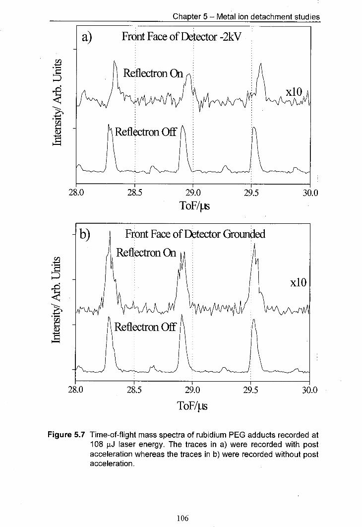
Chapter 5 - Metal ion detachment studies
a) Frnt Face of Detector -2kV
Reflectron On
iw- p Li OJiLIiI
28.0 28.5 29.0 29.5 30.0
ToF/JJs
b) Front Face of Detector Grounded
) Refléctron On
Reflectron Off
x1O
28.0 28.5 29.0 29.5 30.0
ToF4ts
Figure 5.7 Time-of-flight mass spectra of rubidium PEG adducts recorded at 108 pJ laser energy. The traces in a) were recorded with post acceleration whereas the traces in b) were recorded without post acceleration.
106
Chapter 5 - Metal ion detachment studies
The fact that little peak broadening and no retardation are observed for the
neutral fragments formed in PSD of polymer metal ion adducts indicates that the
neutrals observed were formed in a field free environment i.e. in the post-source and
pre-reflectron section of the mass spectrometer.
5.3.3 Altering the reflectron voltage
For this experiment the effect of varying the reflectron voltage on the flight
times of PEG (average molecular weight 1000 Da) adducts was investigated. The
metal ions used to form the adducts were Li and Rb respectively. PEG was chosen,
as it is a well defined polymer in terms of average molecular weight and
polydispersity and because the various metal ion adduct peaks are well separated.
The separation between Li and Rb adducts is 10 Da and the mass separation
between Rb and Na adducts is 18 Da. The Rb and Na adduct mass separation is
an important consideration in these experiments as there very often is some Na
contamination. The mass separation between Rb and Na adducts of PPG for
example is only 4 Da, which makes PPG a comparatively poor choice for these
experiments, as the Na and Rb adduct peaks can overlap. Rb and Li were chosen
for these experiments, as Li adducts do not dissociate under experimental
conditions, whereas Rb adducts do (see section 5.3.1).
All the samples used for these experiments were produced using the aerosol
method. The extraction voltage applied was always +4 W. The reflectron voltage
was varied between 0 and +5 W. The mass spectra presented in this section are the
average of four separate mass spectra, each of which was the summed average of 50
laser shots. Averaging over four spectra was used to improve reproducibility.
107
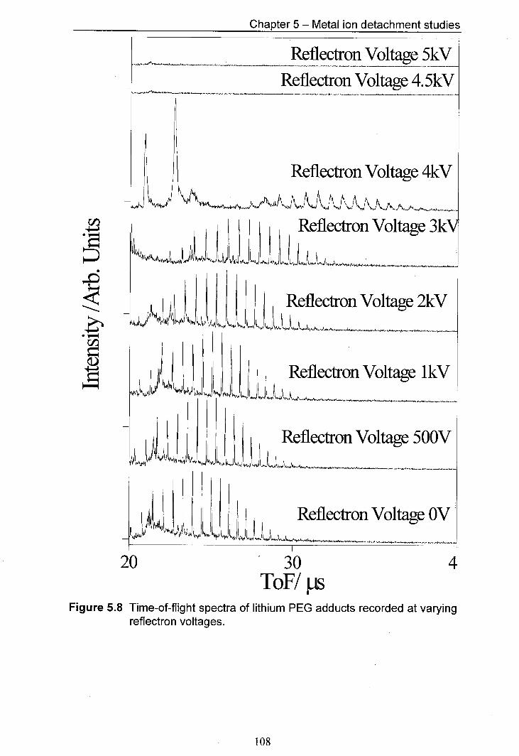
Chapter 5 - Metal ion detachment studies
Reflectron Voltage 5kV
Reflectron Voltage 4.5kV
Reflectron Voltage 4kV
Reflectron Voltage 3k
Reflectron Voltage 2kV
Reflectron Voltage 1 IN
Reflectron Voltage 500V
Reflectron Voltage OV
20 30 4 ToF/ jis
Figure 5.8 Time-of-flight spectra of lithium PEG adducts recorded at varying reflectron voltages.
108
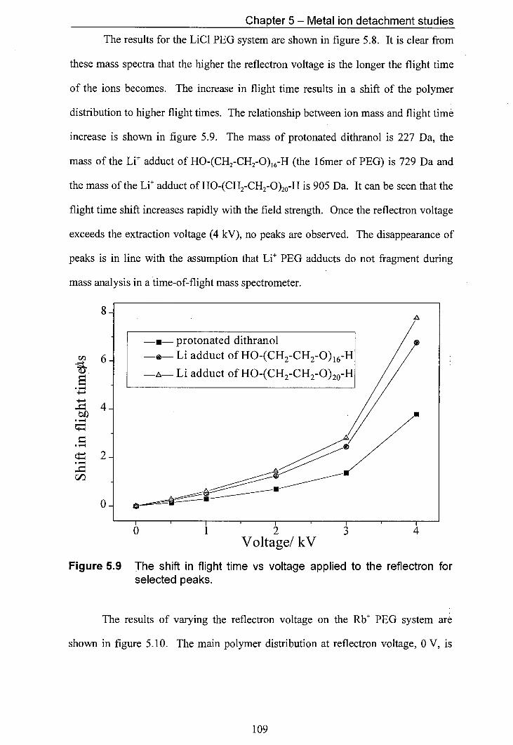
Chapter 5 - Metal ion detachment studies
The results for the LiCl PEG system are shown in figure 5.8. It is clear from
these mass spectra that the higher the reflectron voltage is the longer the flight time
of the ions becomes. The increase in flight time results in a shift of the polymer
distribution to higher flight times. The relationship between ion mass and flight time
increase is shown in figure 5.9. The mass of protonated dithranol is 227 Da, the
mass of the Li adduct of HO-(CH2-CH2-0)16-H (the 16mer of PEG) is 729 Da and
the mass of the Li adduct of HO-(CH2-CH2-0)20-H is 905 Da. It can be seen that the
flight time shift increases rapidly with the field strength. Once the reflectron voltage
exceeds the extraction voltage (4 kV), no peaks are observed. The disappearance of
peaks is in line with the assumption that Li PEG adducts do not fragment during
mass analysis in a time-of-flight mass spectrometer.
8_I I
-.- protonated dithranol
Cn 6 —.—Li adduct of HO-(CH2-CH2-0)16-H
Ir -- Li adduct of HO-(CH2-CH2-0)20-H
2
Voltage! kV
Figure 5.9 The shift in flight time vs voltage applied to the reflectron for selected peaks.
The results of varying the reflectron voltage on the Rb PEG system are
shown in figure 5.10. The main polymer distribution at reflectron voltage, 0 V, is
109
Chapter 5 - Metal ion detachment studies
due to the Rb adduct of PEG, the minor distribution being due to the Na adduct. As
with the Li' PEG adduct ions there is an increase in the flight time of the Rb PEG
adduct ions with increasing reflectron voltage. However, the mass spectra recorded
for reflectron voltages of 4.5 kV and 5 kV are not featureless unlike in the LiCI PEG
case. The peaks observed at 4.5 kV and 5 kV are in the same position as Rb PEG
adduct peaks in the 0 V mass spectrum. Furthermore, both 4.5 kV and 5 kV lie
above the extraction voltage; therefore, any peaks observed in these two mass spectra
must be due to uncharged species. It should also be borne in mind that the neutral
peaks should be present in all mass spectra, as they are not affected by the retarding
effect of the reflectron. In order to show that neutral peaks are indeed present in all
mass spectra, the mass spectra were enlarged (figure 5.11).. In the enlarged mass
spectra lines were included to match the flight times of neutral peaks. It is apparent
that the maximum peak intensities of the neutral peaks in the 4.5 kV and 5 kV mass
spectra do not coincide exactly with the Rb PEG oligomer peaks in the 0 V mass
spectrum. The Rb PEG peaks in the 0 V mass spectrum were produced by a
mixture of ions and neutrals hitting the detector; the ions had a shorter flight time due
to post acceleration (c.f section 5.3.2) than the neutral peaks. Because of the width
of the peaks neutral and ion signals overlap as ion signals were ca ten times more
intense than the neutral signal. Thus the overall peaks produced by the overlap of the
two signal types appear at shorter flight times than the flight times observed for
neutrals alone. Peaks that correspond to neutrals can be seen in all mass spectra
although ion peaks sometimes obscure these peaks. It is worth noting that the
intensity of the neutral peaks does not appear to change with reflectron voltage
indicating that the mechanism for neutral formation is independent of the reflectron
voltage.
110
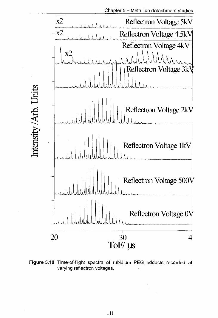
Chapter 5 - Metal ion detachment studies
1%
Reflectron Voltage 5k x2
A A A A A A Reflectron Voltage 4.5k
Reflectron Voltage 4kV x2
Reflectron Voltage 3k
CtJ
Reflectron Voltage 2k
Reflectron Voltage 1 IN
Reflectron Voltage 500
Reflectron Voltage
20 30 4 ToF! s
Figure 5.10 Time-of-flight spectra of rubidium PEG adducts recorded at varying reflectron voltages.
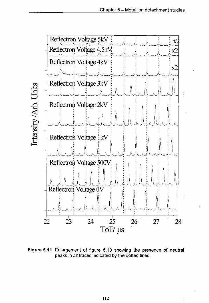
Chapter 5 - Metal ion detachment studies
Reflectron Voltage RV Reflectron V61ta2e 4.5kV
Re&ctron Voltage 4kV
Reflectroñ Voltage 3kV
Reflefroñ Voltage 2kV
Reflectron Voltage I
Reflectron Voltage OOV
HHt Reflèctroij VoRage OV
22 23 24 25 26 27 28 ToF/ps
Figure 5.11 Enlargement of figure 5.10 showing the presence of neutral peaks in all traces indicated by the dotted lines.
112
Chapter 5 - Metal ion detachment studies
This experiment has confirmed that PSD is observed for the Rb adducts of
PEG whereas it is not observed for the Li adducts. Also the peaks seen at high
reflectron voltages for the RbCI PEG sample were confirmed as neutrals.
Furthermore, it has also been shown that the reflectron voltage does not affect the
dissociation of the Rb adducts of PEG.
5.3.4 Experiments on the variation of the laser energy
The effect of laser energy on the formation of neutrals was investigated. The
polymer chosen for these experiments was PEG, for the reasons outlined in section
5.3.3. The four different metal ions used were Li, Nat, K and Rb. It was the aim
of these experiments to ascertain whether at increased laser energies the amount of
fragmentation would increase. If an increase in fragmentation was observed it would
suggest that the internal energy of the polymer metal ion complex was raised. If no
increase in the amount of fragmentation was seen internal energies would appear not
to be sufficiently increased to raise the fragmentation probability.
The samples were prepared using the aerosol method. The laser energy was
varied by means of a neutral density filter. The range of laser energies studied was
from 69 p.J to 108 p.J for PEG with LiC1, NaCl, KC1 and RbC1 and a wider range of
energies for PEG with Li and Rb (76 p.J to 158 p.J). For the lower energy range
experiments (69 j.xJ to 108 tJ) the detector was set to a lower voltage (3.5 kV),
113
Chapter 5 - Metal ion detachment studies
whereas for the higher energies (76 iJ to 158 pJ) the detector voltage was increased
(3.9 kV). Higher detector voltage meant that the sensitivity of the detector was
increased. However, there is a trade off between increased sensitivity and detector
saturation.
5.3.5 Lower laser energy experiments
The results for the 69 j.iJ to 108 pJ experiments are shown in figures 5.12 to
5.19. The mass spectra are shown as waterfall plots to make comparisons easier and
to show up trends. The x and y axes show time-of-flight and signal intensity,
respectively. The laser energy is displayed on the z-axis (NB. The z-axis is not
linear). The range of laser energies and the detector voltage (sensitivity) were
chosen, so that at the lowest laser energy a signal was obtained. The highest laser
energy that could be used was limited by detector saturation.
For the lower laser energy experiment a comparison was made between mass
spectra recorded with the reflectron switched off (ions and neutrals are both detected)
and mass spectra recorded with the reflectron switched on (only neutrals can be
detected) for a range of polymer salt combinations.
114
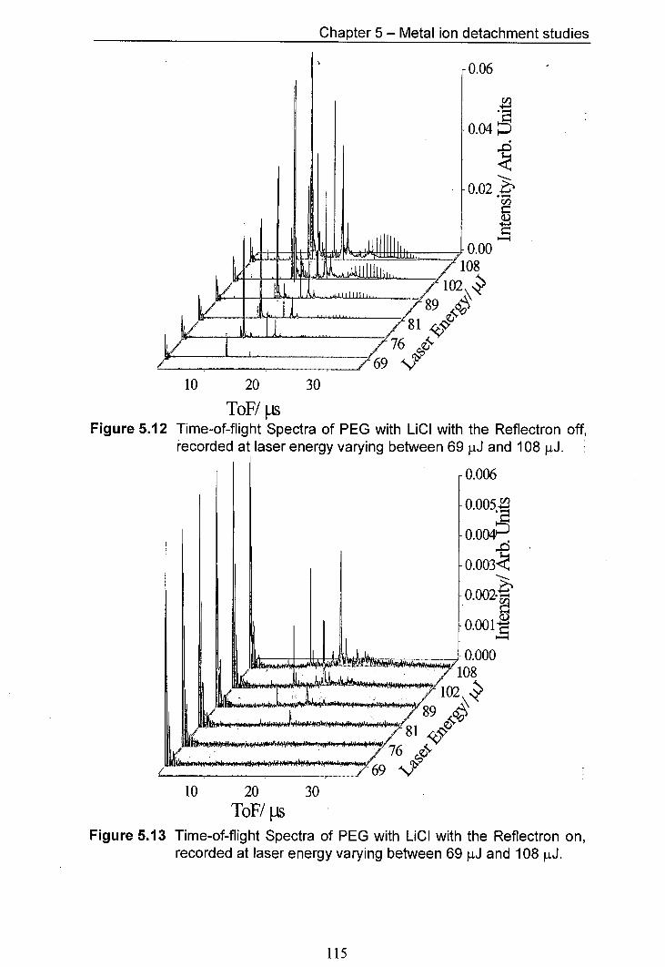
0.005.
0.004
0.003k
0.002-
0.001
0.000 08
[I!IIII
Chapter 5 - Metal ion detachment studies
MR
Cn
44 0.04
0.02
0.00 08
10 20 30
ToF/ is Figure 5.12 Time-of-flight Spectra of PEG with LICI with the Reflectron off,
recorded at laser energy varying between 69 iJ and 108 .iJ.
10 20 30 ToF/s
Figure 5.13 Time-of-flight Spectra of PEG with LiCl with the Reflectron on, recorded at laser energy varying between 69 p.J and 108 [tJ.
115
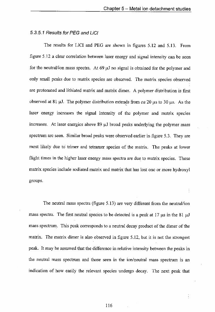
Chapter 5 - Metal ion detachment studies
5.3.5.1 Results for PEG and L1CI
The results for LiC1 and PEG are shown in figures 5.12 and 5.13. From
figure 5.12 a clear correlation between laser energy and signal intensity can be seen
for the neutral/ion mass spectra. At 69 .tJ no signal is obtained for the polymer and
only small peaks due to matrix species are observed. The matrix species observed
are protonated and lithiated matrix and matrix dimer. A polymer distribution is first
observed at 81 j.0. The polymer distribution extends from ca 20 to 30 jis. As the
laser energy increases the signal intensity of the polymer and matrix species
increases. At laser energies above 89 pJ broad peaks underlying the polymer mass
spectrum are seen. Similar broad peaks were observed earlier in figure 5.3. They are
most likely due to trimer and tetramer species of the matrix. The peaks at lower
flight times in the higher laser energy mass spectra are due to matrix species. These
matrix species include sodiated matrix and matrix that has lost one or more hydroxyl
groups.
The neutral mass spectra (figure 5.13) are very different from the neutral/ion
mass spectra. The first neutral species to be detected is a peak at 17 ts in the 81 tJ
mass spectrum. This peak corresponds to a neutral decay product of the dimer of the
matrix. The matrix dimer is also observed in figure 5.12, but it is not the strongest
peak. It may be assumed that the difference in relative intensity between the peaks in
the neutral mass spectrum and those seen in the ion/neutral mass spectrum is an
indication of how easily the relevant species undergo decay. The next peak that
116
Chapter 5 - Metal ion detachment studies
appears in the neutral mass spectrum is the lithiated matrix peak at a time-of-flight of
11.98 pts first seen at a laser energy of 89 p.J. This peak is the strongest peak in
figure 5.12, the next strongest being the protonated matrix peak, which is only
marginally weaker. The protonated matrix peak is not seen in the neutral mass
spectra, even at the highest laser energies. The absence of a protonated matrix signal
in the neutral mass spectrum indicates that the protonated species is less likely to
decay. Also present in the 102 p.J and 108 iJ neutral mass spectra is a signal at a
flight time of 12.57 is corresponding to sodiated matrix which is not seen in the
ion/neutral mass spectra (figure 5.12) as its intensity is too low. It is, however,
observed in figure 5.13 as these mass spectra were magnified by a factor often. The
signal intensity of the neutral signal from sodiated matrix decay products is large
relative to the signal intensity of sodiated matrix species in the ion/neutral mass
spectrum. If the ratio between the sodiated and lithiated matrix peaks was the same
in the figure 5.12 as in figure 5.13, a sizeable peak would have been seen in figure
5.12 for the sodiated matrix. This indicates that sodiated matrix is more likely to
undergo PSD than is the lithiated matrix. The highest laser energy mass spectrum of
figure 5.13 shows a broad feature at a flight time of 24 j.is. This is believed to be due
to the decay products of matrix trimer species. No peaks associated with the polymer
were observed in figure 5.13 which indicates that lithiated PEG does not undergo
extensive PSD under the experimental conditions used.
In summary, the LiC1 PEG mass spectra showed that under standard MALDI
conditions, lithiated PEG does not undergo PSD. The signal intensity of peaks
117
Chapter 5 - Metal ion detachment studies
increases with laser energy over the chosen range of laser energies for all peaks. For
the dithranol matrix, there is a relationship between the intensity of the neutral signal
obtained and the cation attached. The cation to intensity relationship showed that
protonated dithranol was least susceptible to decay, followed by lithiated dithranol
and that sodiated dithranol was the most likely to undergo PSD. It seems reasonable
to suggest that the conversion from adduct to neutral is via the loss of the attached
cation and that the percentage of adducts that decay to neutrals and cations is a
function of the bond strength between the cationic and the neutral part of the adduct.
5.3.52 Results for PEG and Na C/
The mass spectra for NaCl and PEG are presented in figures 5.14 and 5.15.
Figure 5.14 shows the mass spectra recorded with the reflectron off, i.e. showing
both ions and neutrals. The trends observed for the LiCl and PEG system with the
reflectron off (figure 5.12) are seen again. The signal intensity of all peaks increases
as the laser energy is increased. The first peaks to appear at 69 tJ are due to
protonated matrix and sodiated matrix. The signal for the protonated matrix is -
considerably greater than that of its sodiated equivalent. At 76 j.iJ the first sodiated
polymer peaks are observed. At 81 tJ two peaks appear with flight times of 16.15 us
and 16.85 us, respectively. These peaks were assigned as the protonated and
sodiated dithranol dimer. A notable difference between the LiCl PEG spectra
(figure 5.12) and the NaCl PEG mass spectra
118
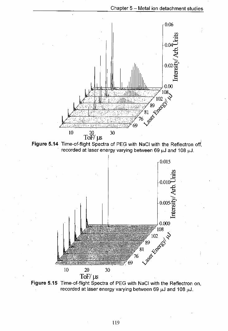
OR
.02k00.02--
0.00 .00 08
15
10 4
05
00
Chapter 5 - Metal ion detachment studies
10 20 30 ToF/jts
Figure 5.14 Time-of-flight Spectra of PEG with NaCl with the Reflectron off, recorded at laser energy varying between 69 11J and 108 J.
10 20 30 ToF/js
Figure 5.15 Time-of-flight Spectra of PEG with NaCl with the Reflectron on, recorded at laser energy varying between 69 p.J and 108 W.
119
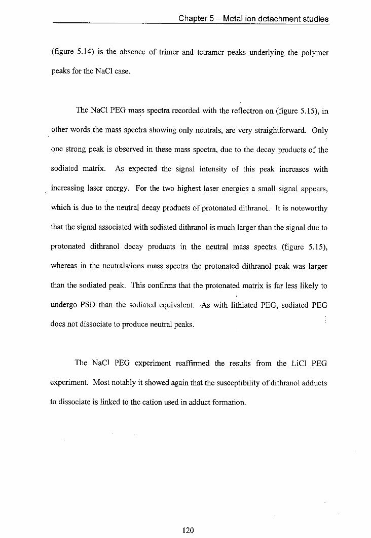
Chapter 5 - Metal ion detachment studies
(figure 5.14) is the absence of trimer and tetramer peaks underlying the polymer
peaks for the NaC1 case.
The NaC1 PEG mass spectra recorded with the reflectron on (figure 5.15), in
other words the mass spectra showing only neutrals, are very straightforward. Only
one strong peak is observed in these mass spectra, due to the decay products of the
sodiated matrix. As expected the signal intensity of this peak increases with
increasing laser energy. For the two highest laser energies a small signal appears,
which is due to the neutral decay products of protonated dithranol. It is noteworthy
that the signal associated with sodiated dithranol is much larger than the signal due to
protonated dithranol decay products in the neutral mass spectra (figure 5.15),
whereas in the neutrals/ions mass spectra the protonated dithranol peak was larger
than the sodiated peak. This confirms that the protonated matrix is far less likely to
undergo PSD than the sodiated equivalent. As with lithiated PEG, sodiated PEG
does not dissociate to produce neutral peaks.
The NaCJ PEG experiment reaffirmed the results from the LiC1 PEG
experiment. Most notably it showed again that the susceptibility of dithranol adducts
to dissociate is linked to the cation used in adduct formation.
120
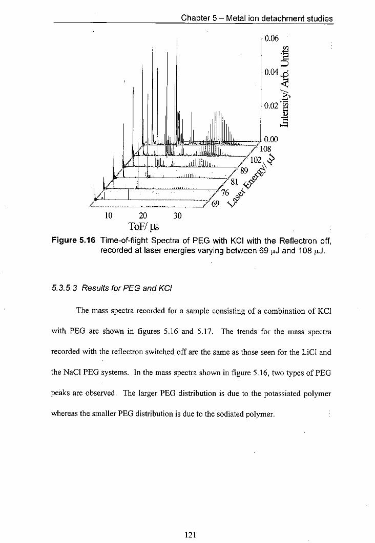
Chapter 5 - Metal ion detachment studies
0.06
0.04 d
0.02
0.00 08
10 20 30
ToF/ Is Figure 5.16 Time-of-flight Spectra of PEG with KCI with the Reflectron off,
recorded at laser energies varying between 69 j.1J and 108 .tJ.
5.3.5.3 Results for PEG and KCI
The mass spectra recorded for a sample consisting of a combination of KCJ
with PEG are shown in figures 5.16 and 5.17. The trends for the mass spectra
recorded with the reflectron switched off are the same as those seen for the L1C1 and
the NaCl PEG systems. In the mass spectra shown in figure 5.16, two types of PEG
peaks are observed. The larger PEG distribution is due to the potassiated polymer
whereas the smaller PEG distribution is due to the sodiated polymer.
121
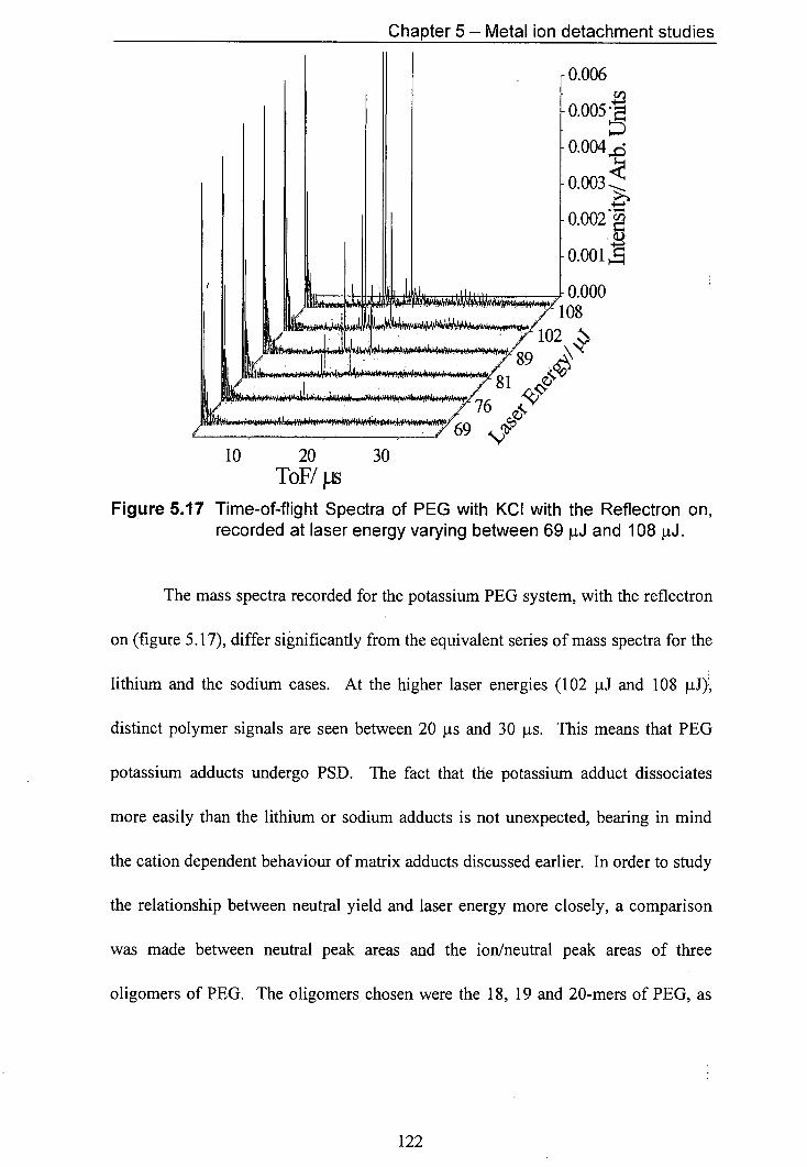
0.006
0.005
0.004
0.003
0.002 LQ
'M 0.001
0.000 08
Chapter 5 - Metal ion detachment studies
10 20 30 ToF/ s
Figure 5.17 Time-of-flight Spectra of PEG with KCI with the Reflectron on, recorded at laser energy varying between 69 tJ and 108 j.iJ.
The mass spectra recorded for the potassium PEG system, with the reflectron
on (figure 5.17), differ significantly from the equivalent series of mass spectra for the
lithium and the sodium cases. At the higher laser energies (102 p.J and 108 J),
distinct polymer signals are seen between 20 ts and 30 is. This means that PEG
potassium adducts undergo PSD. The fact that the potassium adduct dissociates
more easily than the lithium or sodium adducts is not unexpected, bearing in mind
the cation dependent behaviour of matrix adducts discussed earlier. In order to study
the relationship between neutral yield and laser energy more closely, a comparison
was made between neutral peak areas and the ion/neutral peak areas of three
oligomers of PEG. The oligomers chosen were the 18, 19 and 20-mers of PEG, as
122
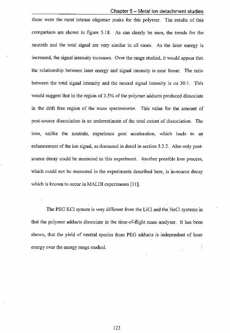
Chapter 5 - Metal ion detachment studies
these were the most intense oligomer peaks for this polymer. The results of this
comparison are shown in figure 5.18. As can clearly be seen, the trends for the
neutrals and the total signal are very similar in all cases. As the laser energy is
increased, the signal intensity increases. Over the range studied, it would appear that
the relationship between laser energy and signal intensity is near linear. The ratio
between the total signal intensity and the neutral signal intensity is ca 30:1. This
would suggest that in the region of 3.5% of the polymer adducts produced dissociate
in the drift free region of the mass spectrometer. This value for the amount of
post-source dissociation is an underestimate of the total extent of dissociation. The
ions, unlike the neutrals, experience post acceleration, which leads to an
enhancement of the ion signal, as discussed in detail in section 5.3.2. Also only post-
source decay could be measured in this experiment. Another possible loss process,
which could not be measured in the experiments described here, is in-source decay
which is known to occur in MALDI experiments [11].
The PEG KCI system is very different from the L1C1 and the NaCl systems in
that the polymer adducts dissociate in the time-of-flight mass analyser. It has been
shown, that the yield of neutral species from PEG adducts is independent of laser
energy over the energy range studied.
123
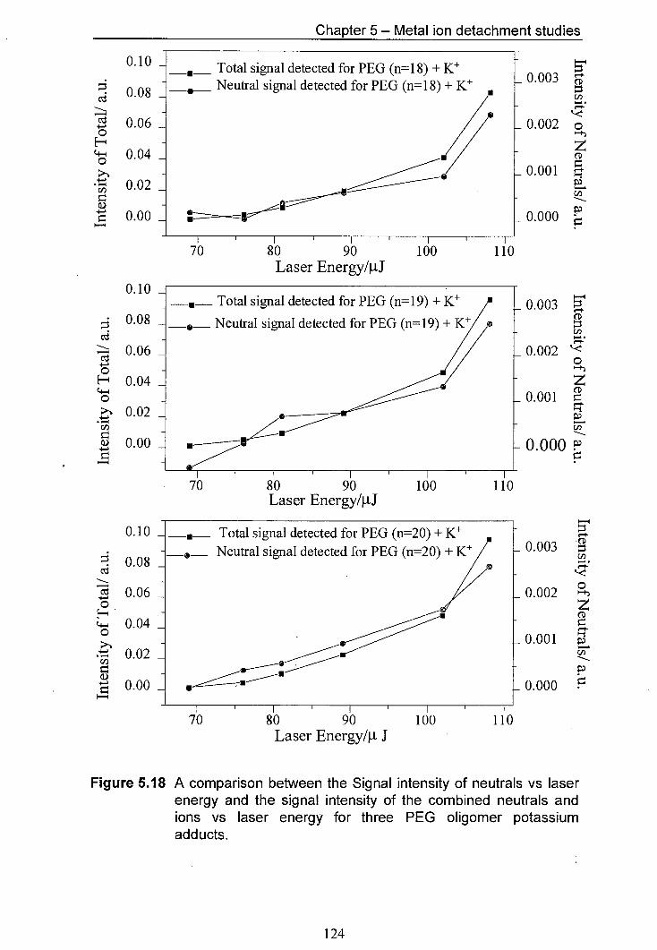
Chapter 5 - Metal ion detachment studies
Total • 0.10_ - signal detected for PEG (n=1 8) + K - 0.003 CD
0.08 Neutral signal detected for PEG (n--18) + K - riD
It 0.06 //•
0.002 0 0 H
./ 0.04 CD
- 0.001 0.02rID -
0.00 -
(ID
- 0.000
Laser Energy! jtJ 0.10
0.06 0 H 0.04 0
0.02
0.00
. Total signal detected for PEG (n=19) + K
-j Neutral signal detected for PEG (n= 19) + K 0.003
0.002 0
0.001
riD
70 80 90 100 110 Laser Energy4LJ
0.10
0.08 03
+cd 0.06
0.04
I
.b 0.02
0.00
Total signal detected for PEG (n=20) + K ._ Neutral signal detected for PEG (n=20) + K 0.003
:sxixiii
70 80 90 100 110 Laser Energy/j.i J
Figure 5.18 A comparison between the Signal intensity of neutrals vs laser energy and the signal intensity of the combined neutrals and ions vs laser energy for three PEG oligomer potassium adducts.
124
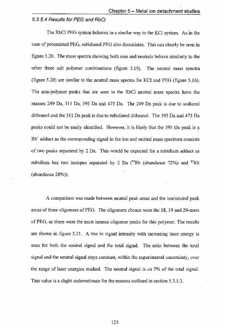
Chapter 5 - Metal ion detachment studies
5.3.5.4 Results for PEG and RbCI
The RbC1 PEG system behaves in a similar way to the KC1 system. As in the
case of potassiated PEG, rubidiated PEG also dissociates. This can clearly be seen in
figure 5.20. The mass spectra showing both ions and neutrals behave similarly to the
other three salt polymer combinations (figure 5.19). The neutral mass spectra
(figure 5.20) are similar to the neutral mass spectra for KC1 and PEG (figure 5.16).
The non-polymer peaks that are seen in the RbC1 neutral mass spectra have the
masses 249 Da, 311 Da, 395 Da and 475 Da. The 249 Da peak is due to sodiated
dithranol and the 311 Da peak is due to rubidiated dithranol. The 395 Da and 475 Da
peaks could not be easily identified. However, it is likely that the 395 Da peak is a
Rb adduct as the corresponding signal in the ion and neutral mass spectrum consists
of two peaks separated by 2 Da. This would be expected for a rubidium adduct as
rubidium has two isotopes separated by 2 Da (85Rb (abundance 72%) and 17 R
(abundance 28%)).
A comparison was made between neutral peak areas and the ion/neutral peak
areas of three oligomers of PEG. The oligomers chosen were the 18, 19 and 20-mers
of PEG, as these were the most intense oligomer peaks for this polymer. The results
are shown in figure 5.21. A rise in signal intensity with increasing laser energy is
seen for both the neutral signal and the total signal. The ratio between the total
signal and the neutral signal stays constant, within the experimental uncertainty, over
the range of laser energies studied. The neutral signal is ca 5% of the total signal.
This value is a slight underestimate for the reasons outlined in section 5.3.5.3.
125
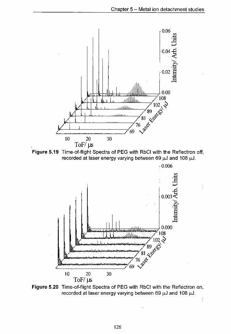
Chapter 5 - Metal ion detachment studies
0.06 ci)
0.04
0.02
0.00 08
10 20 30 T0F/tis
Figure 5.19 Time-of-flight Spectra of PEG with RbCI with the Reflectron off, recorded at laser energy varying between 69 j.1J and 108 pJ.
[sI•IIr.i
ci)
0.003k
0.000 08
10 20 30 ToF/ p.s
Figure 5.20 Time-of-flight Spectra of PEG with RbCI with the Reflectron on, recorded at laser energy varying between 69 i.J and 108 pJ.
126
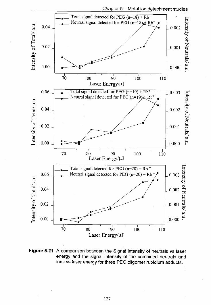
CD 0.003
0.002
CD (\ .(\JJ1
-# J
Oil "1
C,)
:ix.isxi
II
CD 0.003
Chapter 5 - Metal ion detachment studies
Cd 0.04
0.002 CD
Cd
0.02
0.001 CD
C,) C-fl
i)
0.00
0.000
'Is
0.04
0.02
0.00
/0 80 90 100 110 Laser Energy/jiJ
Total signal detected for PEG (n=19) + Rb Neutral signal detected for PEG (n=19)Rb
/0 80 90 100 110 Laser Energy/J
Total signal detected for PEG (n=20) + Rb +
J Neutral signal detected for PEG (n=20) + Rb +
0 0.04
0.002 H
CD
0.02
0.001
0.00
0.000
/0 80 90 100 110 Laser Energy! jtJ
Figure 5.21 A comparison between the Signal intensity of neutrals vs laser energy and the signal intensity of the combined neutrals and ions vs laser energy for three PEG oligomer rubidium adducts.
/ 127
Chapter 5 - Metal ion detachment studies
5.3.5.5 Conclusions of the lower laser energy experiments
Some very clear trends were observed in these experiments. The signal
intensity for all species observed increased with increasing laser energy. The
generation of neutrals was found to be dependent on the type of cation used in adduct
formation. For dithranol, it was found that protonated dithranol did not dissociate
under experimental conditions. All the metal ion adducts of dithranol did dissociate
to varying extents. The lithium adduct dissociated least readily, followed by the
sodium adduct, then the potassium adduct and finally the rubidium adduct
dissociated most readily. The degree of dissociation is linked directly to the size of
the attached cation. The smaller the cation, the more stable the adduct. The same
trend was observed for the metal ion adducts of PEG. The Li and Na adducts of
PEG did not dissociate under experimental conditions. Potassiated and sodiated PEG
did both dissociate. The fraction of the adducts that dissociated did not vary with
applied laser energy. A larger percentage of the rubidium adduct of PEG dissociated
than of the potassium adduct of PEG (5% and 3.5%, respectively). The extent to
which the K and Rb adducts of PEG dissociate appears to be independent of the
laser energy. This would suggest that the internal energy of these adducts is not
greatly increased by the increase in laser energy. An increase in internal energy
would be expected to increase the proportion of adducts that undergo decay.
128
Chapter 5 - Metal ion detachment studies
5.5.6 Higher laser energy experiments
For these experiments the range of laser energies was extended, going from
76 ltJ to 158 pJ. Also the detector gain was increased, giving a more sensitive
detector response. Two samples were studied, namely PEG (average molecular
weight 1000 Da) with a dithranol matrix and LiC1 as the salt and the same polymer
and matrix with RbCl as the salt. The samples were prepared using the aerosol
method. The aim of these experiments was to determine whether or not the strongly
bound lithium adduct of PEG would dissociate at these higher laser energies. As a
comparison the effects on the Rb PEG system were also studied under these
conditions. These experiments also give an illustration of the response of the
microchannel plate detector under these conditions.
The results for the LiC1 PEG combination are shown in figures 5.22 and 5.23.
The mass spectra presented in figure 5.22 were recorded with the reflectron switched
off, allowing charged and uncharged species to be detected. The peaks at 20 lts and
above are due to lithiated PEG. Between laser energies of 76 J and 108 1.iJ, the
trend observed is the same as for the lower energy experiments described earlier. At
132 l.J the polymer peak intensity drops sharply and the peaks broaden. At 158 j.iJ
the polymer signal disappears almost completely. The lower mass peaks below
15 lts increase in intensity with increasing laser energy. Figure 5.23 shows the
neutral mass spectrum for the LiCI PEG system. It is clear that in the neutral mass
129
Chapter 5 - Metal ion detachment studies
spectra, all peaks increase in intensity with increasing laser energy. However, even
at 158 tJ no neutral peaks associated with the lithium PEG adduct were observed.
Figure 5.24 shows the ion/neutral mass spectra for PEG and RbC1. The peaks
at flight times of 20 j.is and above are due to polymer adducts. Rubidium and sodium
adducts are seen, the rubidium PEG adducts being the strongest polymer distribution.
The intensity of the polymer peaks increases with laser energy up to an energy of
89 1.0. At laser energies of 108 tJ and higher the polymer peak intensity decreases
and the peak width increases. The polymer peaks in the mass spectrum recorded at
158 pJ have been reduced to a low intensity continuum. The lower mass peaks
observed in figure 5.24 (below 15 ts) increase with laser energy over the whole
energy range. In the mass spectrum recorded at 158 jxJ there is a group of peaks
centred at 5 ts which overlap and are so intense that they go off scale. Figure 5.25
shows the neutral mass spectra for the RbC1 PEG system. Polymer peaks are seen in
all mass spectra. The polymer peak height increases with increasing laser energy up
to a laser energy of 132 tJ. The polymer peak heights of the 158 tJ mass spectrum
are comparable to the equivalent peaks in the 132 j.tJ mass spectrum. The lower mass
peaks, below 20 ts, increase in signal intensity with laser energy up to 132 j.iJ, and
the peak height decreases in the 158 j.tJ mass spectrum. The peak widths always
increase with increasing laser energy.
130
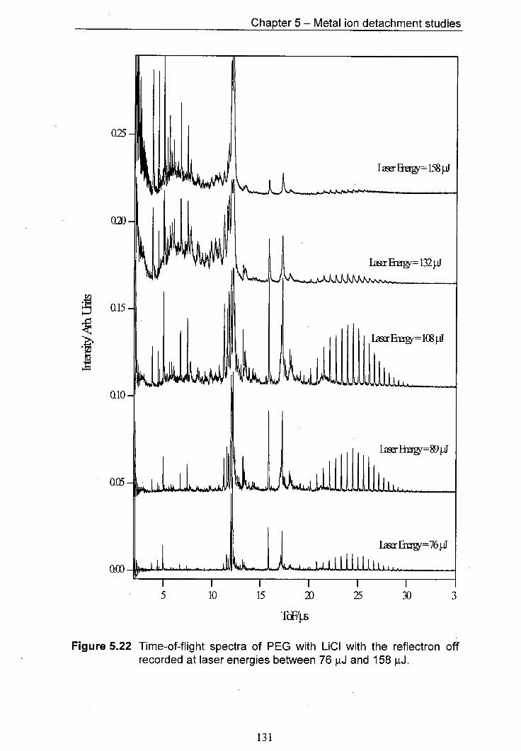
Chapter 5 - Metal ion detachment studies
LaBu= 158 tJ
[I1
Rm
gam
21 22 1 MOM I. 110
5 10 15 2D 25 30 3
Figure 5.22 Time-of-flight spectra of PEG with LiCI with the reflectron off recorded at laser energies between 76 pJ and 158 pJ.
ma
no W
131
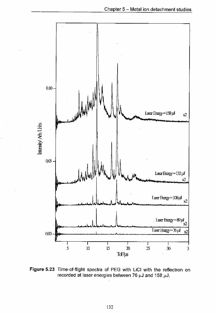
Nm
Chapter 5 - Metal ion detachment studies
5 10 15 2J 25 30 3 TF4
Figure 5.23 Time-of-flight spectra of PEG with L1CI with the reflectron on recorded at laser energies between 76 VtJ and 158 W.
132
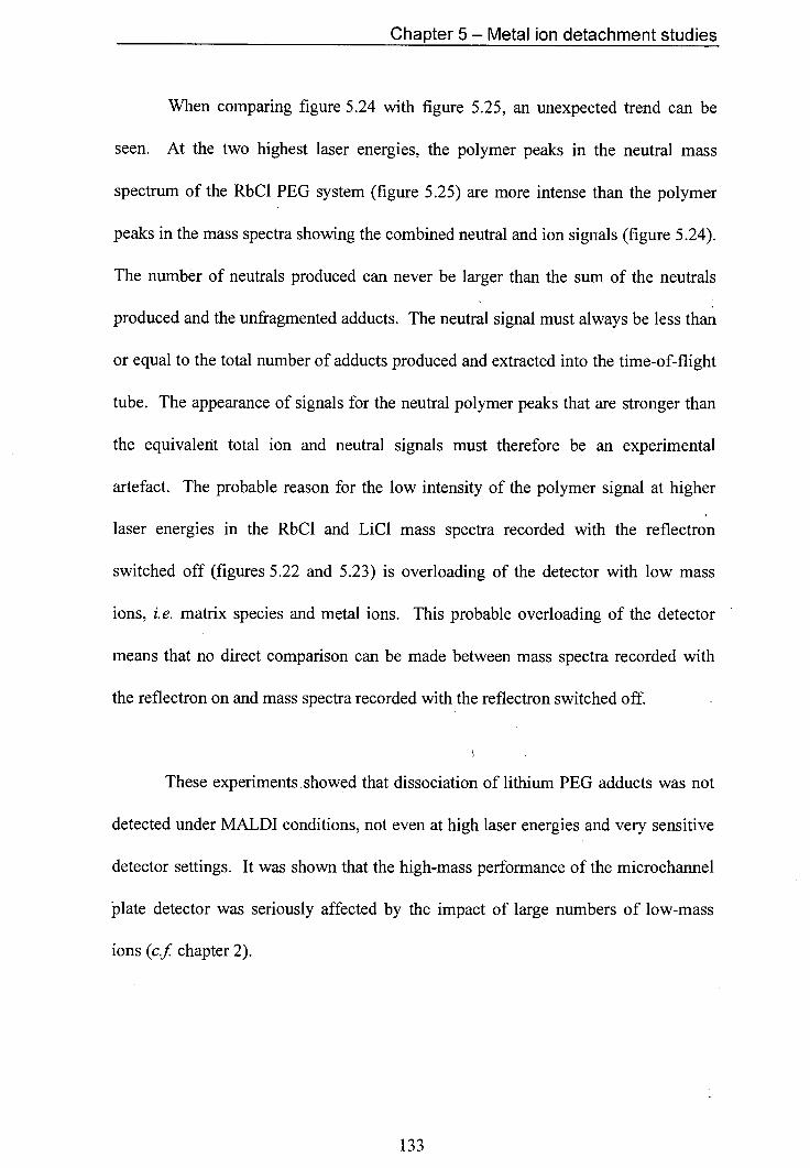
Chapter 5 - Metal ion detachment studies
When comparing figure 5.24 with figure 5.25, an unexpected trend can be
seen. At the two highest laser energies, the polymer peaks in the neutral mass
spectrum of the RbCl PEG system (figure 5.25) are more intense than the polymer
peaks in the mass spectra showing the combined neutral and ion signals (figure 5.24).
The number of neutrals produced can never be larger than the sum of the neutrals
produced and the unfragmented adducts. The neutral signal must always be less than
or equal to the total number of adducts produced and extracted into the time-of-flight
tube. The appearance of signals for the neutral polymer peaks that are stronger than
the equivalent total ion and neutral signals must therefore be an experimental
artefact. The probable reason for the low intensity of the polymer signal at higher
laser energies in the RbC1 and LiC1 mass spectra recorded with the reflectron
switched off (figures 5.22 and 5.23) is overloading of the detector with low mass
ions, i.e. matrix species and metal ions. This probable overloading of the detector
means that no direct comparison can be made between mass spectra recorded with
the reflectron on and mass spectra recorded with the reflectron switched off.
These experiments showed that dissociation of lithium PEG adducts was not
detected under MALDI conditions, not even at high laser energies and very sensitive
detector settings. It was shown that the high-mass performance of the microchannel
plate detector was seriously affected by the impact of large numbers of low-mass
ions (c.f chapter 2).
133
Chapter 5 - Metal ion detachment studies
0.25
Lagx Bwg= 158 pJ
MI LaBtigy= 132 tJ
I
LaB= 108 tJ
0.10
in
[Bg'=76tJ
5 10 15 2D 25 30 3
TF4s
Figure 5.24 Time-of-flight spectra of PEG with RbCI with the reflectron off recorded at laser energies between 76 .iJ and 158 jtJ.
134
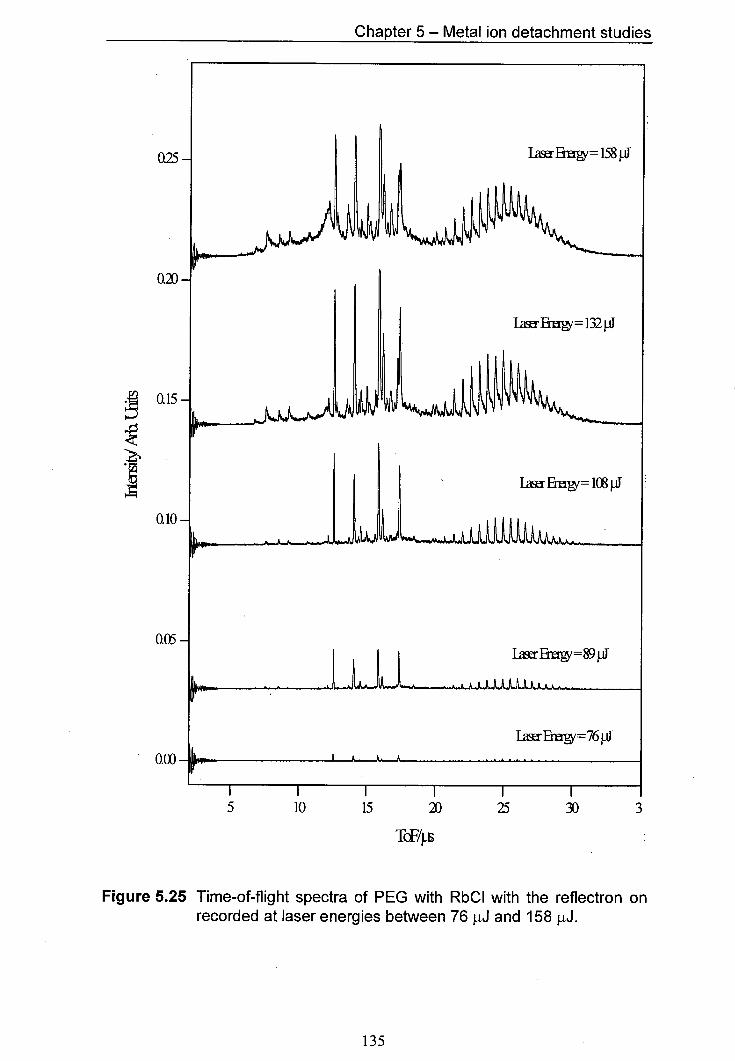
Chapter 5 - Metal ion detachment studies
0.25
faqx 158 W
L Hug = 132 Iff
0.10
[aBi=76 jtJ
[IriI]
5 10 15 2D 25 30 3
Tci
Figure 5.25 Time-of-flight spectra of PEG with RbCI with the reflectron on recorded at laser energies between 76 j.iJ and 158 .iJ.
135

Chapter 5 - Metal ion detachment studies
5.5.7 Effect of fragmentation on the mass distribution of polydisperse
polymers
One of the greatest problems in the mass determination of synthetic polymers
using MALDI is the poor agreement sometimes observed between average masses of
polydisperse polymers determined using traditional techniques and the average
molecular mass arrived at using MALDI [12,13]. Various reasons for the average
molecular weight discrepancies have been put forward [14,15]. The possibility of
different adduct dissociation rates has, however, not yet been addressed. An apparent
shift in molecular weight would be observed if high-mass oligomer adducts were
more prone to dissociation than low-mass oligomers or vice versa. The experiment
outlined below aims to show whether the dissociation rate of oligomer adducts is
mass dependent and whether this could be a factor affecting the accurate
determination of average molecular weights of polymers by MALDI mass
spectrometry.
In the following experiments three positive ion detection modes were used.
The linear detector, with the reflectron switched off, was used to examine the
molecular weight distribution of a polymer obtained, when intact adducts and those
that have fragmented in the field free drift region of the mass spectrometer, are both
detected. In this reflectron-off mode, every oligomer adduct that has entered the
time-of-flight detector is detected regardless of whether it has dissociated or not
(see figure 5.1).
136
Chapter 5 - Metal ion detachment studies
The linear detector with the reflectron switched on was used to examine the
molecular weight distribution of the neutral dissociation products of polymer adducts
(see figure 5.2).
The reflectron detector was used to determine the fraction of oligomer
adducts that did not dissociated by the time they had reached the linear detector.
This was possible as only ionised species could be reflected by the reflectron and
hence be detected using the reflectron detector (see figure 5.2).
The samples studied consisted of dithranol as the matrix, KC1 as the salt and
PEG, as the polymer. Different molecular weight PEG samples were used. The PEG
samples used were PEG 1000 (average molecular weight 1000 Da) and PEG 2000
(average molecular weight 2000 Da). Both of these PEG samples were
monodisperse. Another sample was prepared in which two monodisperse PEG
samples were combined to make up a more polydisperse sample. The PEG samples
in the mixture were PEG 1000 and PEG 3400, with average molecular weights of
1000 Da and 3400 Da, respectively. These polymer samples were mixed in a 1:9
ratio, PEG 1000 to PEG 3400. This mixing ratio was chosen to give a bimodal mass
distribution, with two maxima of roughly similar intensities. All samples were
prepared using the aerosol method. The gain on the detectors was varied for all
137

Chapter 5 - Metal ion detachment studies
modes to give comparable signal intensities in order to facilitate comparison of mass
spectra and to produce a similar detector response.
No significant differences were found in the polymer mass distributions
between the three different types of mass spectra recorded for PEG 1000 and PEG
2000. As both PEG 1000 and PEG 2000 polymer distributions cover a
comparatively small mass range only a small difference in dissociation behaviour of
the high-mass adducts and the low-mass adducts of this oligomer range would be
expected.
The results for the experiment for which a more polydisperse polymer sample
was produced by mixing PEG 1000 and PEG 3400 are shown in figure 5.26. All
three mass spectra exhibit a bimodal polymer distribution, the maxima of which are
centred on 1000 Da and 3400 Da, respectively. The polymer distribution in
figure 5.26 a contains some intense peaks due to matrix trimer and tetramer species
between 750 Da and 1250 Da. These matrix peaks are more intense than the polymer
peaks in this part of the mass spectrum. There is no apparent obvious difference
between the polymer distributions in the three mass spectra shown in figure 5.26.
This indicates that, for the system investigated, there is no significant difference in
the extent of dissociation between high-mass and low-mass oligomers. Polymer
adduct dissociation would appear not to be a major factor to the skewing of polymer
mass distributions of polydisperse polymers often seen in MALDI mass
spectrometry.
138
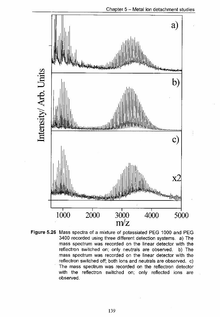
Chapter 5 - Metal ion detachment studies
Cl)
1000 2000 3000 4000 5000 m1z
Figure 5.26 Mass spectra of a mixture of potassiated PEG 1000 and PEG 3400 recorded using three different detection systems. a) The mass spectrum was recorded on the linear detector with the reflectron switched on; only neutrals are observed. b) The mass spectrum was recorded on the linear detector with the reflectron switched off; both ions and neutrals are observed. c) The mass spectrum was recorded on the reflectron detector with the reflectron switched on; only reflected ions are observed.
139
Chapter 5 - Metal ion detachment studies
5.4 Conclusions
The work outlined in this chapter investigates the production of neutral
species through the dissociation of adducts in the field free drift region of a time-of-
flight mass spectrometer in polymer MALDI experiments. It was shown that certain
polymer metal ion adducts dissociate post-source. The proportion of the polymer
metal ion adducts which dissociated was dependent on the metal ion. It was found
that for alkali metal adducts of polymers, the lithium and sodium adducts did not
dissociate, whereas the potassium and rubidium adducts did dissociate. Potassium
adducts dissociated to a lesser extent than rubidium adducts, suggesting that the
higher the charge density of the cation, the more stable the adduct. This dissociation
behaviour was found to be similar for a range of different polymers, namely
poly(ethylene glycol), poly(propylene glycol) and poly(methyl methacrylate). A
more detailed study of poly(ethylene glycol) revealed that the dissociation rate of the
potassium and rubidium adducts was independent of laser energy over an energy
range of 69 tJ to 108 .iJ. This suggests that the increase in laser energy did not
greatly increase the average internal energy of the polymer adduct. It was found that
over this laser energy range ca 3.5% of potassium adducts and 5% of rubidium
adducts underwent PSD. The extent of dissociation of potassium adducts of
poly(ethylene glycol) does not significantly change over the mass range of 673 Da to
4545 Da. The trend in alkali metal ion size compared with the extent of
fragmentation would suggest that the post-source decay seen is dependent on the
metal ion oligomer bond. The neutrals observed were most probably formed through
the loss of the metal ion from the polymer metal adduct ion.
140
Chapter 5 - Metal ion detachment studies
5.5 References
B. Stahl, M. Steup, M. Karas and F. Hillenkamp, Anal. Chem., 63, 1463-1468 (1991) K. 0. Bornsen, M. Scharr, E. Gassmaim and V. Steiner, Biol. Mass Spectrom. 20, 471-475 (1991) I. A. Mowat and R. J. Donovan, Rapid Commun. Mass Spectrom., 9, 82-90 (1995) H. Rashidezadeh and B. C. Guo, I Am. Soc. Mass Spectrom., 9, 724-730 (1998) M. J. Deery, K. R. Jennings, C. B. Jasieczek, D. M. Haddleton, A.T. Jackson, H. T. Yates and J. H. Scrivens, Rapid Commun. Mass Spectrom., 11, 57-62 (1997) C. K. L. Wong and T. W. D. Chan, Rapid Commun. Mass Spectrom., 11, 513-519(1997) C. F. Liens and R. M. O'Malley, Rapid Commun. Mass Spectrom., 6, 564-570 (1992) P. A. Dean and R. M. O'Malley, Rapid Commun. Mass Spectrom., 7, 53-57 (1993) J. H. Scrivens, A. T. Jackson, H. T. Yates, M. R. Green, G. Critchley, J. Brown, R. H. Bateman, M. T. Bowers and J. Gidden, mt. I. Mass Spectrom. Ion Proc., 165, 363-375 (1997) A. Westman, G. Brinkmalm and D. F. Barofsky, mt. J Mass Spectrom. Ion Proc., 169/170, 79-87 (1997) D. C. Reiber, T. A. Grover and R. S. Brown, Anal. Chem., 70, 673-683 (1998) R. S. Lehrle and D. S. Sarson, Rapid Commun. Mass Spectrom., 9, 91-92 (1995) K. Martin, J. Spickermann, H. J. Rader and K. Mullen, Rapid Commun. Mass Spectrom., 10, 1471-1474 (1996) D. C. Schriemer and L. Li, Anal. Chem., 69, 4169-4175 (1997) D. C. Schriemer and L. Li, Anal. Chem., 69, 4176-4183 (1997)
141
Chapter 6 - Delayed extraction experiments
Chapter 6— Delayed extraction experiments
6.1 Introduction
Delayed extraction techniques have come into wide use over recent years
[1,2,3]. Delayed extraction is often employed to improve the resolution of time-of-
flight mass spectrometers. In the work described in this chapter, delayed extraction
was not used for this purpose but it was used to investigate cation attachment
reactions and initial velocity distributions in the MALDI source. Mowat et al. [4]
and Wang and co-workers [5] have previously described similar experiments into
cation attachment. In both these experiments an increase in signal intensity was seen
with increasing delay time for adduct ion formation up to a maximum intensity, after
which the signal intensity dropped off again.
An increase in signal intensity was observed for peptides [5] and
polymers [4]. The maximum intensities were recorded at the following delay times,
500 ns for polystyrene with Ag [4], 700 ns for poly(propylene glycol) with Na [4]
and between 340 ns and 550 ns for gramicidin S with K [5]. These results were
interpreted as evidence for gas-phase adduct formation, with the increase in signal
intensity with delay time, being due to continued adduct formation in the source
region during the time delay. In a more recent paper Schanen et al. demonstrated
142
Chapter 6 - Delayed extraction experiments
efficient gas-phase adduct formation in supersonic beam experiments [6]. Hoberg
and co-workers, through use of a layered sample deposition technique provided
further evidence for gas-phase cationisation [7]. In this experiment, the matrix and
analyte were sandwiched between two salt layers, each salt layer consisting of a
different salt. Only cations from the bottom salt layer attached to the analyte. This
selective attachment was seen as evidence for gas-phase reactions as, after laser
ablation, the metal ions from the bottom layer would pass through the matrix analyte
layer, whereas the top layer metal ions would not have an opportunity to interact in
such a way. There are indications from work on whether photochemical or thermal
processes occur during MALDI that different mechanisms operate for proton and
metal-ion attachment [8]. Proton adducts were only observed if photochemical
processes occurred, whereas metal ion adducts were observed even if only thermal
processes were possible [8]. These observations would suggest that photoexcited
matrix species are not necessary for metal ion adduct formation. The possibility of
thermal desorption was interpreted as evidence for preformation of metal ion adducts
in the solid phase [8]. Recent work by Knochenmuss et al. suggests that adduct
formation occurs 'promptly' after the laser shot and that two photoexcited matrix
molecules are required to bring about adduct formation [10,11]. It seems probable
that more than one channel exists for adduct formation and that some, if not all, the
mechanisms proposed play a part.
The aim of the work described in this chapter was to investigate the adduct
formation for the polystyrene silver system using delayed ion extraction. A similar
approach was taken to that of Mowat [4,9] but there were several important
143
Chapter 6 - Delayed extraction experiments
differences; first a novel sample preparation method was employed, giving improved
reproducibility and secondly the work was carried out using a linear TOF mass
spectrometer. The effect that salt concentration had on the ionisation behaviour was
investigated. The aim was to test the hypothesis of Knochenmuss and co-workers
that a minimum of two photoexcited matrix molecules were required to bring about
ionisation [10,11]. At low salt concentrations, the probability of two photoexcited
matrix molecules being nearest neighbours in the solid is high and therefore the
proposed prompt ionisation mechanism can occur. However, at very high salt
concentrations, it is far less likely that two photoexcited matrix molecules are next to
each other, as salt molecules make up a large number of a given matrix molecule's
nearest neighbours. Consequently, it is reasonable to expect fewer gas-phase cation
adductions at low salt concentrations than in the high salt concentration scenario, as
the probability of prompt reactions occurring is greatly increased at low salt
concentrations.
6.2 Experimental
The power supply to the sample holder in the source had to be modified to
carry out delayed extraction experiments. A schematic illustration of the delayed
extraction configuration of the instrument is shown in figure 6.1. A potential of up to
5 kV was delivered by a high voltage power supply (model PS350, Stanford
Research Systems, Inc.), driving a fast high voltage push-pull switch (Behike,
Germany). The switch was triggered by a pulse generator (Lyons Instruments),
which produced a square wave. The trigger for the pulse generator was provided by
the synchronous output of the laser. A time delay of from 0 to 2 ts between the
144
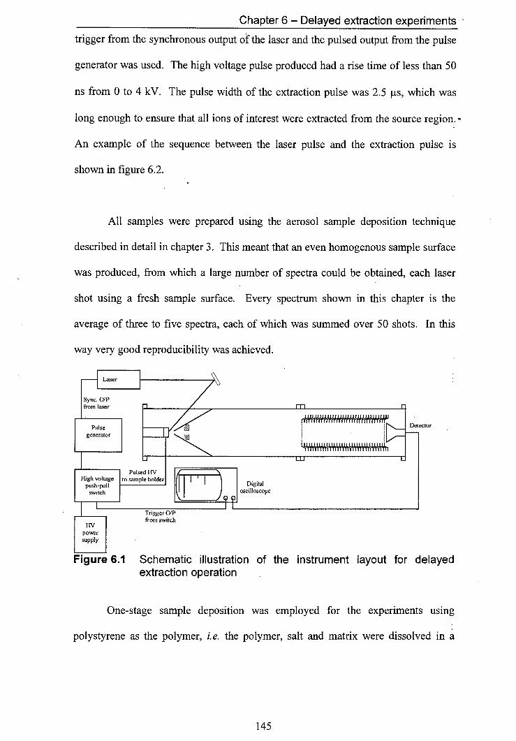
Chapter 6 - Delayed extraction experiments
trigger from the synchronous output of the laser and the pulsed output from the pulse
generator was used. The high voltage pulse produced had a rise time of less than 50
ns from 0 to 4 kV. The pulse width of the extraction pulse was 2.5 ts, which was
long enough to ensure that all ions of interest were extracted from the source region..
An example of the sequence between the laser pulse and the extraction pulse is
shown in figure 6.2.
All samples were prepared using the aerosol sample deposition technique
described in detail in chapter 3. This meant that an even homogenous sample surface
was produced, from which a large number of spectra could be obtained, each laser
shot using a fresh sample surface. Every spectrum shown in this chapter is the
average of three to five spectra, each of which was summed over 50 shots. In this
way very good reproducibility was achieved.
ector
Figure 6.1 Schematic illustration of the instrument layout for delayed extraction operation
One-stage sample deposition was employed for the experiments using
polystyrene as the polymer, i.e. the polymer, salt and matrix were dissolved in a
[1
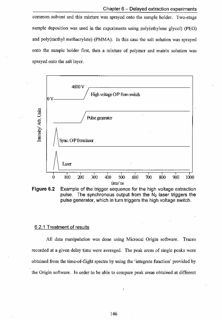
Chapter 6 - Delayed extraction experiments
common solvent and this mixture was sprayed onto the sample holder. Two-stage
sample deposition was used in the experiments using poly(ethylene glycol) (PEG)
and poly(methyl methacrylate) (PMMA). In this case the salt solution was sprayed
onto the sample holder first, then a mixture of polymer and matrix solution was
sprayed onto the salt layer.
__ High voltage 0/P from switch
Pulse generator
Sc. 0/P from laser
Laser
0 100 200 300 400 500 600 700 800 900 1000 tin-e/ as
Figure 6.2 Example of the trigger sequence for the high voltage extraction pulse. The synchronous output from the N2 laser triggers the pulse generator, which in turn triggers the high voltage switch.
6.2.1 Treatment of results
All data manipulation was done using Microcal Origin software. Traces
recorded at a given delay time were averaged. The peak areas of single peaks were
obtained from the time-of-flight spectra by using the 'integrate function' provided by
the Origin software. In order to be able to compare peak areas obtained at different
146
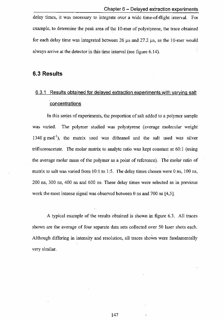
Chapter 6 - Delayed extraction experiments
delay times, it was necessary to integrate over a wide time-of-flight interval. For
example, to determine the peak area of the 1 0-mer of polystyrene, the trace obtained
for each delay time was integrated between 26 ts and 27.2 .is, as the 1 0-mer would
always arrive at the detector in this time interval (see figure 6.14).
6.3 Results
6.3.1 Results obtained for delayed extraction experiments with varying salt
concentrations
In this series of experiments, the proportion of salt added to a polymer sample
was varied. The polymer studied was polystyrene (average molecular weight
1340 g mol 1), the matrix used was dithranol and the salt used was silver
trifluoroacetate. The molar matrix to analyte ratio was kept constant at 60:1 (using
the average molar mass of the polymer as a point of reference). The molar ratio of
matrix to salt was varied from 10:1 to 1:5. The delay times chosen were 0 ns, 100 ns,
200 ns, 300 ns, 400 ns and 600 ns. These delay times were selected as in previous
work the most intense signal was observed between 0 ns and 700 ns [4,5].
A typical example of the results obtained is shown in figure 6.3. All traces
shown are the average of four separate data sets collected over 50 laser shots each.
Although differing in intensity and resolution, all traces shown were fundamentally
very similar.
147
0 500 1000 1500 2000 250
I
Chapter 6 - Delayed extraction experiments
nlz Figure 6.3 Effect of delayed ion extraction on the MALDI mass spectra of
polystyrene. In the bottom trace no delay between the laser shot and ion extraction was used. For the other traces, a delay of between 100 ns and 600 ns was used, as shown. The matrix used was dithranol and the salt used was AgCF3CO2. The matrix to salt ratio was 1 to 5.
148
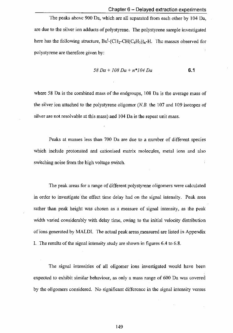
Chapter 6 - Delayed extraction experiments
The peaks above 900 Da, which are all separated from each other by 104 Da,
are due to the silver ion adducts of polystyrene. The polystyrene sample investigated
here has the following structure, But(CH2CH(C6H5))H. The masses observed for
polystyrene are therefore given by:
58 Da + 108 Da + n*104 Da 6.1
where 58 Da is the combined mass of the endgroups, 108 Da is the average mass of
the silver ion attached to the polystyrene oligomer (N. B. the 107 and 109 isotopes of
silver are not resolvable at this mass) and 104 Da is the repeat unit mass.
Peaks at masses less than 700 Da are due to a number of different species
which include protonated and cationised matrix molecules, metal ions and also
switching noise from the high voltage switch.
The peak areas for a range of different polystyrene oligomers were calculated
in order to investigate the effect time delay had on the signal intensity. Peak area
rather than peak height was chosen as a measure of signal intensity, as the peak
width varied considerably with delay time, owing to the initial velocity distribution
of ions generated by MALDI. The actual peak areas,measured are listed in Appendix
I. The results of the signal intensity study are shown in figures 6.4 to 6.8.
The signal intensities of all oligomer ions investigated would have been
expected to exhibit similar behaviour, as only a mass range of 600 Da was covered
by the oligomers considered. No significant difference in the signal intensity versus
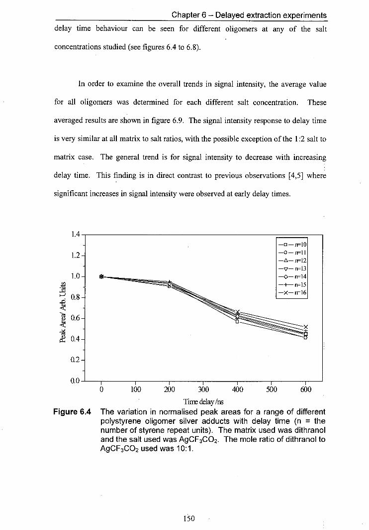
Chapter 6 - Delayed extraction experiments
delay time behaviour can be seen for different oligomers at any of the salt
concentrations studied (see figures 6.4 to 6.8).
In order to examine the overall trends in signal intensity, the average value
for all oligomers was determined for each different salt concentration. These
averaged results are shown in figure 6.9. The signal intensity response to delay time
is very similar at all matrix to salt ratios, with the possible exception of the 1:2 salt to
matrix case. The general trend is for signal intensity to decrease with increasing
delay time. This finding is in direct contrast to previous observations [4,5] where
significant increases in signal intensity were observed at early delay times.
1.4
1.2
1.0
-D-ilO —O—n11 --n=12 —v—n=13 --n14
-X- n16
0.2
MI 0 100 200 300 400 500 600
Yin delay /ns Figure 6.4 The variation in normalised peak areas for a range of different
polystyrene oligomer silver adducts with delay time (n = the number of styrene repeat units). The matrix used was dithranol and the salt used was AgCF3CO2. The mole ratio of dithranol to AgCF3CO2 used was 10:1.
150
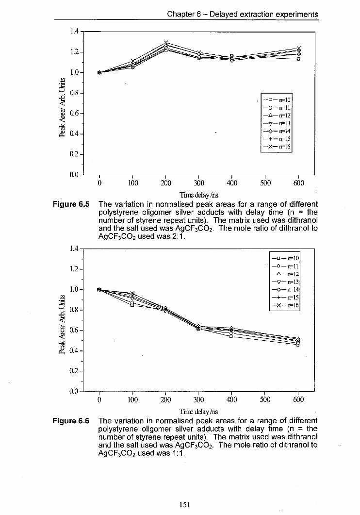
Chapter 6 - Delayed extraction experiments
1.2
1IJ
0.8 —°—ii=1O —O—n11
0.6 —t—n=12 —v— n=13
0.4
--n=14 —+— n=15 —X— n16
xi 0 100 200 300 400 500 600
Tin delay /ns Figure 6.5 The variation in normalised peak areas for a range of different
polystyrene oligomer silver adducts with delay time (n = the number of styrene repeat units). The matrix used was dithranol and the salt used was AgCF3CO2. The mole ratio of dithranol to AgCF3CO2 used was 2:1.
1.2
1.0
0.8
1 0.6 0.4
—D—ri=1O
_O_flrlI
--n12 —v—n=13 -- n=14 —+— n=15 —X— n=16
0.2
He 0 100 200 300 400 500 600
Time delay Ins Figure 6.6 The variation in normalised peak areas for a range of different
polystyrene oligomer silver adducts with delay time (n = the number of styrene repeat units). The matrix used was dithranol and the salt used was AgCF3CO2. The mole ratio of dithranol to AgCF3CO2 used was 1:1.
151
Chapter 6 - Delayed extraction experiments
0 100 200 300 400 500 600
Tine delay Ins Figure 6.7 The variation in normalised peak areas for a range of different
polystyrene oligomer silver adducts with delay time (n = the number of styrene repeat units). The matrix used was dithranol and the salt used was AgCF3CO2. The mole ratio of dithranol to AgCF3CO2 used was 1:2.5.
1.4
1.2
1.0
- -0- n10 - —O—n11
-- n=12 —v—n=13 --n14 -+- rrl5
- —X— n16
MI 0 100 200 300 400 500 600
Tmie delay Ins Figure 6.8 The variation in normalised peak areas for a range of different
polystyrene oligomer silver adducts with delay time (n = the number of styrene repeat units). The matrix used was dithranol and the salt used was AgCF3CO2. The mole ratio of dithranol to AgCF3CO2 used was 1:5.
1.2
10,
0.8
0.6
0.4
0.2
0.8
0.6
0.4
0.2
152
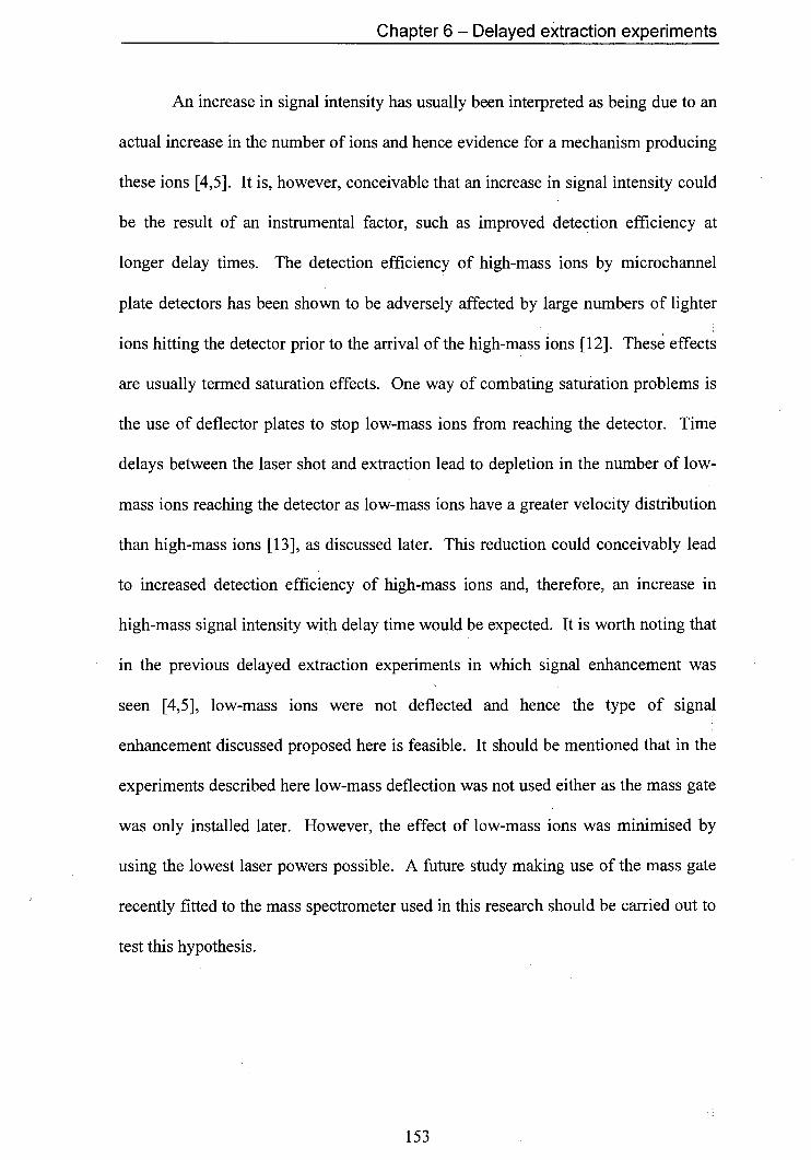
Chapter 6 - Delayed extraction experiments
An increase in signal intensity has usually been interpreted as being due to an
actual increase in the number of ions and hence evidence for a mechanism producing
these ions [4,5]. It is, however, conceivable that an increase in signal intensity could
be the result of an instrumental factor, such as improved detection efficiency at
longer delay times. The detection efficiency of high-mass ions by microchannel
plate detectors has been shown to be adversely affected by large numbers of lighter
ions hitting the detector prior to the arrival of the high-mass ions [12]. These effects
are usually termed saturation effects. One way of combating saturation problems is
the use of deflector plates to stop low-mass ions from reaching the detector. Time
delays between the laser shot and extraction lead to depletion in the number of low-
mass ions reaching the detector as low-mass ions have a greater velocity distribution
than high-mass ions [13], as discussed later. This reduction could conceivably lead
to increased detection efficiency of high-mass ions and, therefore, an increase in
high-mass signal intensity with delay time would be expected. It is worth noting that
in the previous delayed extraction experiments in which signal enhancement was
seen [4,5], low-mass ions were not deflected and hence the type of signal
enhancement discussed proposed here is feasible. It should be mentioned that in the
experiments described here low-mass deflection was not used either as the mass gate
was only installed later. However, the effect of low-mass ions was minimised by
using the lowest laser powers possible. A future study making use of the mass gate
recently fitted to the mass spectrometer used in this research should be carried out to
test this hypothesis.
153

Chapter 6 - Delayed extraction experiments
The study presented here shows an overall decrease in signal intensity with
increasing delay time. This decrease can be accounted for by two main loss
pathways. First, as ions formed by MALDI can have considerable initial velocities,
ions can be lost by moving away from the extraction region of the source. Typical
average initial ion velocities reported for analyte ions (i.e. ions with mass >1000 Da)
are in the range of 500 to 1000 m s_i [13,14,15,16 and 171. The diameter of the
extraction optics used for this experiment used was 2 mm. An ion with a velocity of
1000 m s 1 (typical velocity reported for analyte ions) covers a distance of 1 mm in
1 [ts. Therefore, it can be assumed that drift of ions out of the extraction region • is
one of the factors leading to a decrease in signal intensity with increasing delay time.
Another possible loss mechanism is the collision induced and/or spontaneous decay
of polymer ions, for instance through the loss of the metal cation. In-source decay
has been reported [18]. Collisions between ions and neutrals are probable in the
source region; also ions can have large internal energies which can lead to
dissociation.
The results presented here do not point clearly to any specific ionisation
mechanism. However, they show that for the system studied, delayed extraction did
not lead to an increase in signal intensity, which would suggest that gas-phase
reactions taking place after the laser shot do not play an important part in the adduct
ion formation mechanism. Of course gas-phase reaction may still be taking place;
however, the number of ions produced in this way must be smaller than the number
of ions lost through decay/non-detection.
154
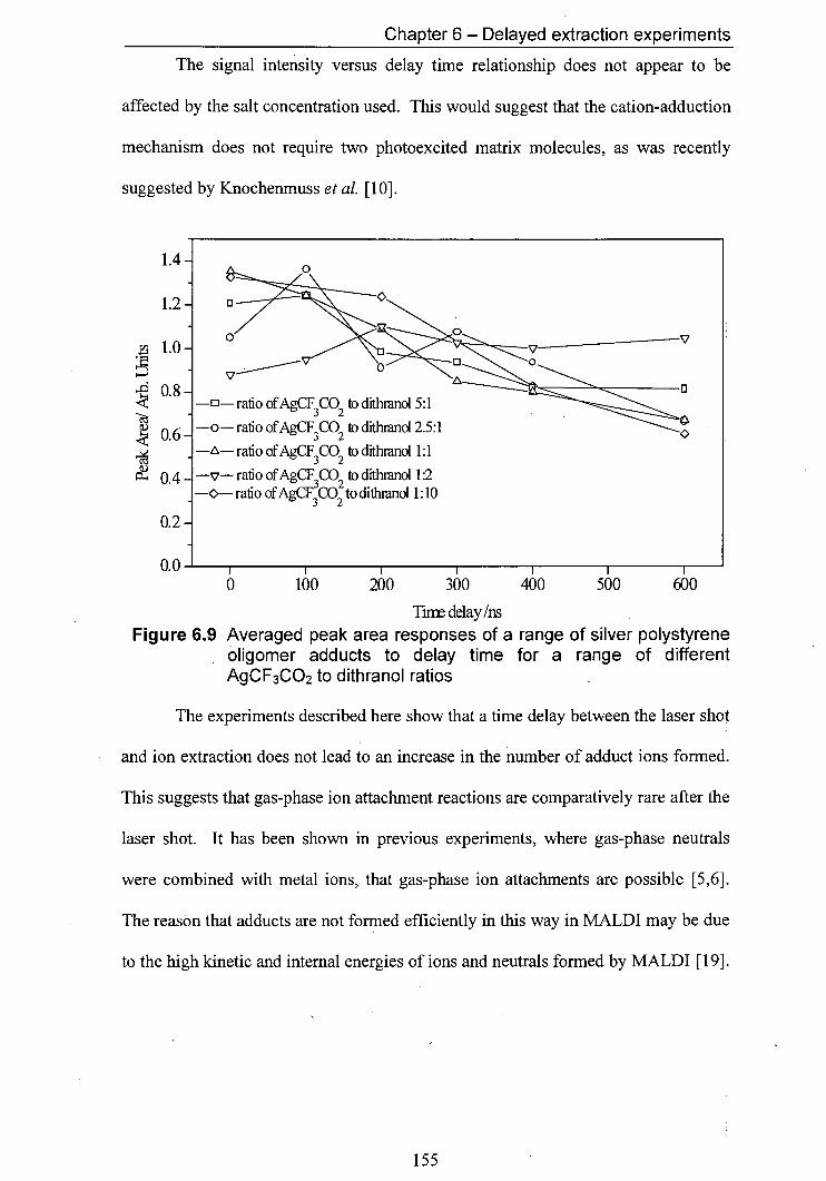
1.0
0.8
0.6
0.4
1.4
1.2
-0-
-0-
-- ratio ofAgCF3CO2 to dithranol 1:1 —v—ratio 0fAgCF3CO2 to dithranol 1:2 —c>-- ratio ofAgCF3CO2 to dithianol 1:10
Chapter 6 - Delayed extraction experiments
The signal intensity versus delay time relationship does not appear to be
affected by the salt concentration used. This would suggest that the cation-adduction
mechanism does not require two photoexcited matrix molecules, as was recently
suggested by Knochenmuss et al. [10].
0.2
no 0 100 200 300 400 500 600
Yam delay Ins Figure 6.9 Averaged peak area responses of a range of silver polystyrene
oligomer adducts to delay time for a range of different AgCF3CO2 to dithranol ratios
The experiments described here show that a time delay between the laser shot
and ion extraction does not lead to an increase in the number of adduct ions formed.
This suggests that gas-phase ion attachment reactions are comparatively rare after the
laser shot. It has been shown in previous experiments, where gas-phase neutrals
were combined with metal ions, that gas-phase ion attachments are possible [5,6].
The reason that adducts are not formed efficiently in this way in MALDI may be due
to the high kinetic and internal energies of ions and neutrals formed by MALDI [19].
155
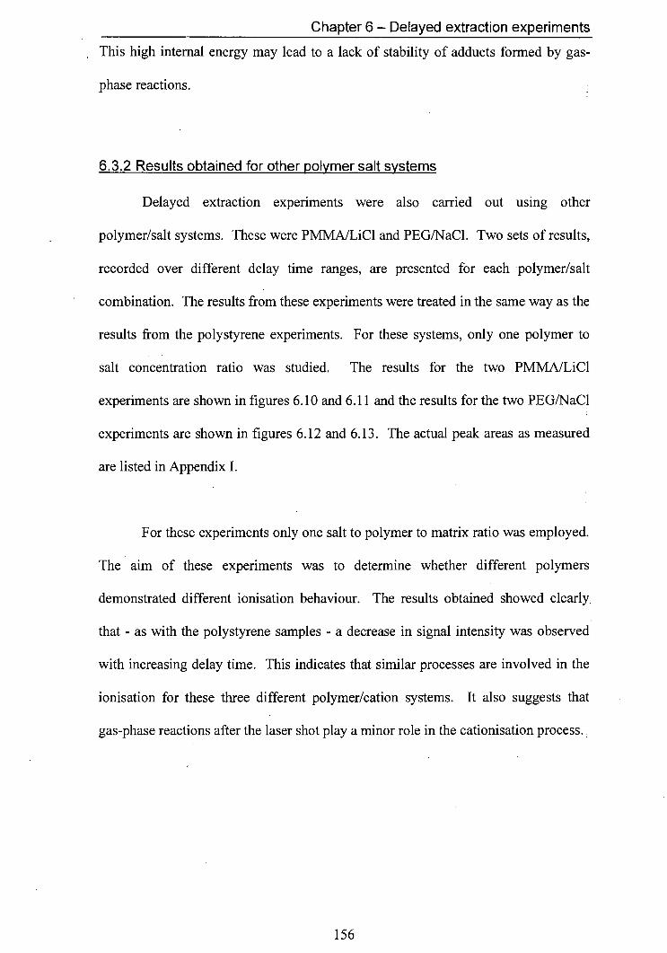
Chapter 6 - Delayed extraction experiments
This high internal energy may lead to a lack of stability of adducts formed by gas-
phase reactions.
6.3.2 Results obtained for other polymer salt systems
Delayed extraction experiments were also carried out using other
polymer/salt systems. These were PMMA/LiC1 and PEG/NaCl. Two sets of results,
recorded over different delay time ranges, are presented for each polymer/salt
combination. The results from these experiments were treated in the same way as the
results from the polystyrene experiments. For these systems, only one polymer to
salt concentration ratio was studied. The results for the two PMMA/LiC1
experiments are shown in figures 6.10 and 6.11 and the results for the two PEG/NaCl
experiments are shown in figures 6.12 and 6.13. The actual peak areas as measured
are listed in Appendix I.
For these experiments only one salt to polymer to matrix ratio was employed.
The aim of these experiments was to determine whether different polymers
demonstrated different ionisation behaviour. The results obtained showed clearly.
that - as with the polystyrene samples - a decrease in signal intensity was observed
with increasing delay time. This indicates that similar processes are involved in the
ionisation for these three different polymer/cation systems. It also suggests that
gas-phase reactions after the laser shot play a minor role in the cationisation process.
156
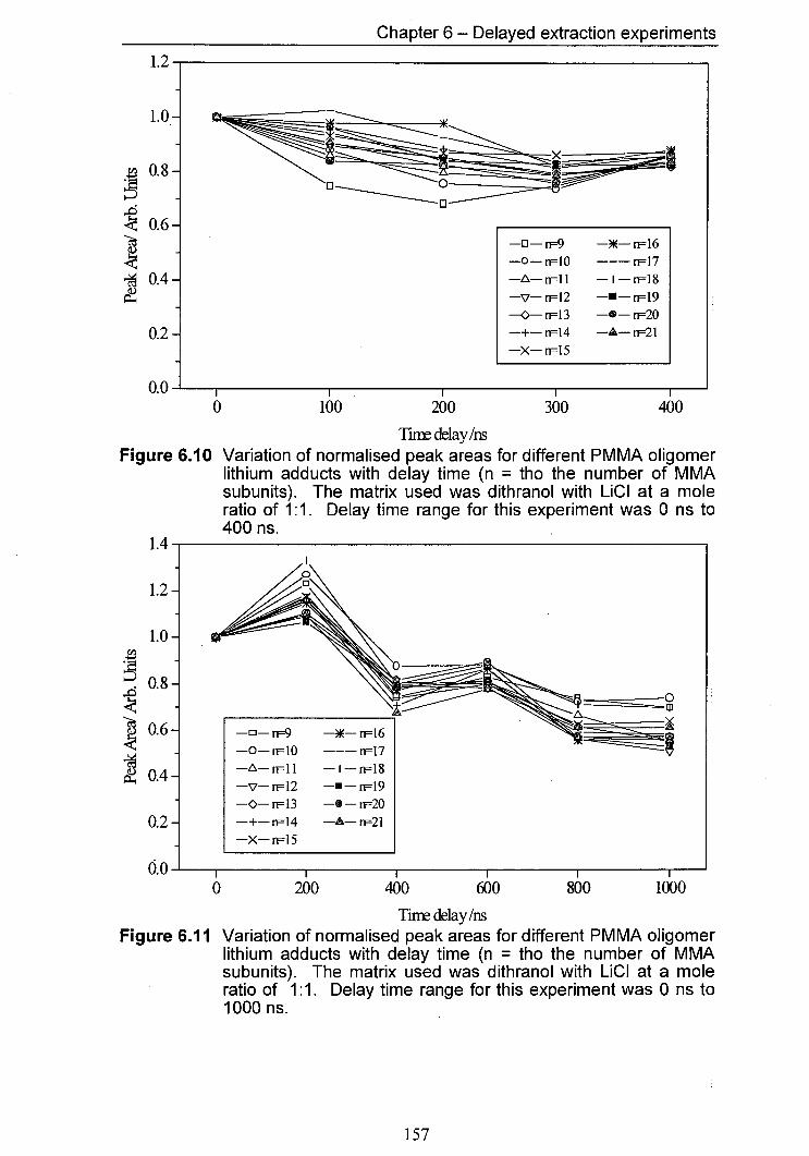
Chapter 6 - Delayed extraction experiments
irni
0.8
-D-n=9 —)IE—n=16 —O—n10 ---n=17
- --n11 —I----n=18 —v—n=12 —U—w19 --n=13 --rF20
- —+—ri14 —A—n=21 —X—ri15
0.2
no 0 100 200 300 400
Time delay Ins Figure 6.10 Variation of normalised peak areas for different PMMA oligomer
lithium adducts with delay time (n = tho the number of MMA subunits). The matrix used was dithranol with L1CI at a mole ratio of 1:1. Delay time range for this experiment was 0 ns to 400 ns.
1.4
--n11 —v—n12 —.—n=19 --n13 —@—n=20 -+- n14 -A- n=21 —x— n15
0 200 400 600 800 1000
Tine delay Ins Figure 6.11 Variation of normalised peak areas for different PMMA oligomer
lithium adducts with delay time (n = tho the number of MMA subunits). The matrix used was dithranol with LiCI at a mole ratio of 1:1. Delay time range for this experiment was 0 ns to 1000 ns.
1.2
1.0
0.8
0.6
0.4
0.2
157

Chapter 6 - Delayed extraction experiments
1.2
- -- n34 —NE— n=44 —v—n=36 ---n46 —G--n38 -I-n=48
- —+—n=40 —U—n=50 —X—n42 n=52
- I
0 100 200 300 400
Time delay/ns Figure 6.12 Variation of normalised peak areas for different PEG oligomer
sodium adducts with delay time (n = tho the number of subunits). The matrix used was dithranol and the salt used was NaCl at a mole ratio of 1:1. Delay time range for this experiment was 0 ns to 400 ns.
12
1.1
1.0
0.9
0.8
0.6
0.5
0.4
0.2
0.1
0.0 0 100 200 300 400 500 600 700 800 900 1000
Time delay/ns Figure 6.13 Variation of normalised peak areas for different PEG oligomer
sodium adducts with delay time (n = the the number of subunits). The matrix used was dithranol with NaCl at a mole ratio of 1:1. Delay time range for this experiment was 0 ns to 1000 ns.
0.6
0.4
02
MI
0.7
0.3
-13
- _13nr32 —X—n=44 —O—n=34 —)K— n=46 --n36 ---n=48 —v—n=38 —I—n50 —G—n=40 —.—n=52
- —+—n=42
158
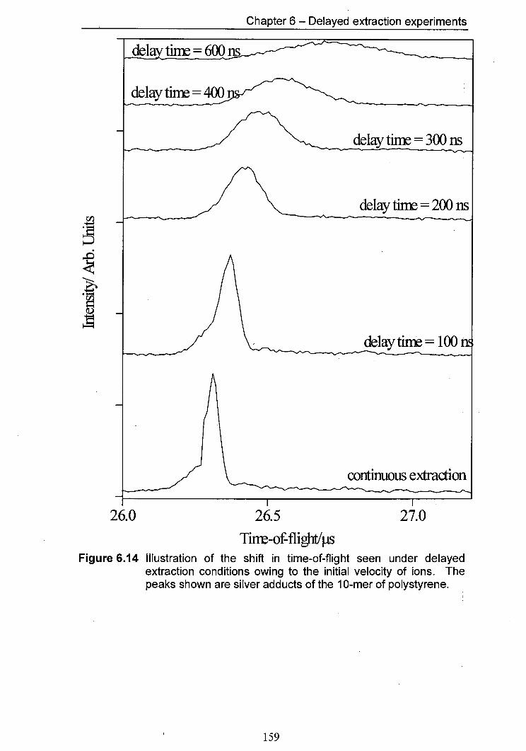
Chapter 6 - Delayed extraction experiments
tin=
delay tint = 400
E1LIL =1J T&Y
delay tin=200ns
I
delay tin= 100
continuous extraction
26.0 26.5 27.0
Tim-of-flight/ps Figure 6.14 Illustration of the shift in time-of-flight seen under delayed
extraction conditions owing to the initial velocity of ions. The peaks shown are silver adducts of the 1 0-mer of polystyrene.
WN
Chapter 6 - Delayed extraction experiments
6.3.3 Initial ion velocities
It was observed in the delayed extraction experiments outlined above that the
peak positions of polymer adducts changed with delay time. The peak-position shift
is illustrated in figure 6.14. As can clearly be seen the peak maxima shift to higher
flight times with time delay. It is also noticeable that the peak width increases
noticeably with delay time. Both these phenomena are direct consequences of the
kinetic energy imparted to the ions during the MALDI process. The increase in
flight time when a time delay is used is due to the ions moving away from the
repeller owing to their initial velocity. The movement of ions away from the sample
holder during the time delay means that they do not experience the full accelerating
potential. As would be expected, the ions do not move at a uniform velocity. This
leads to the peak broadening observed, i.e. some ions travel further from the repeller
than others and therefore their flight time is increased more. A simple computer
model (not shown here) indicated that the initial ion velocities were in the range of
500 in s-1 to 1500 in s-1, which is in good agreement with published data [13,14].
6.4 Conclusions
The experiments described in this chapter show that the number of polymer
adduct ions detected decrease when a time delay between the laser shot and ion
extraction is used. This decrease in signal intensity is more marked at longer delay
times. No evidence for increased adduct yield with time delay was found, contrary
to previously published work. Possible reasons for this discrepancy were discussed.
160
Chapter 6— Delayed extraction experiments
The signal intensity to delay time response was unaffected by salt
concentration even at very high salt concentrations suggesting that the ionisation
process can operate when the probability of two photoexcited matrix molecules being
nearest neighbours is small.
The initial velocity of ions generated using MALDI was clearly noticeable by
an increase in time-of-flight of ions when a time delay was used between ion
extraction and the laser shot.
161
Chapter 6 - Delayed extraction experiments
6.5 References
M. L. Vestal, P. Juhasz and S. A. Martin, Rapid Commun. Mass Spectrom., 9, 1044-1050 (1995) R. M. Whittal and L. Li, Anal. Chem., 67,1950-1954 (1995) U. Bahr, J. Stahl-Zeng, E. Gleitsmann and M. Karas, I Mass Spectrom., 32, 1111-1116 (1997) I. A. Mowat, R. J. Donovan and R. J. Maier, Rapid Commun. Mass Spectrom., 11, 89-98 (1997) B. H. Wang, K. Dreisewerd, U. Bahr, M. Karas and F. Hillenkamp, I Am. Soc. Mass Spectrom., 4, 393-398 (1993) P. Schanen, D. Yang, R. Weinkauf and E. W. Schiag, mt. I Mass Spectrom. Ion Proc., 167/168, 447-470 (1997) A. —M. Hoberg, D. M. Haddleton and P. J. Derrick, Eur. Mass Spectrom., 3, 471-473 (1997) H. Ehring, C. Costa, P. A. Demirev and B. U. R. Sundqvist, Rapid Commun. Mass Spectrom., 10, 821-824 (1996) "Synthetic polymer analysis using matrix assisted laser desorption/ ionisation time-of-flight mass spectrometry", I. A. Mowat, PhD thesis, The University of Edinburgh (1995). R. Knochenmuss, F. Dubois, M. J. Dale and R. Zenobi, Rapid Commun. Mass Spectrom., 10, 871-877 (1996) R. Knochenmuss, V. Karbach, U. Wiesli, K. Breuker and R. Zenobi, Rapid Commun. Mass Spectrom., 12, 529-534 (1998) A. Westman, G. Brinkmalm and D. F. Barofsky, mt. I Mass Spectrom. Ion Proc., 169/170, 79-87 (1997) V. Bokelmann, B. Spengler and R. Kaufmann, Eur. Mass Spectrom., 1, 81-93 (1995) T. —W. D. Chan, I. Thomas, A. W. Colburn and P. J. Derrick, Chem. Phys. Lett., 222, 579-585 (1994) T. Huth-Fehre and C. H. Becker, Rapid Commun. Mass Spectrom., 5, 378-382. (1991) R. C. Beavis and B. T. Chait, Chem. Phys. Lett., 181, 479-484 (1991) Y. Pan and R. J. Cotter, Org. Mass Spectrom., 27, 3-8 (1992) D. C. Reiber, T. A. Grover and R. S. Brown, Anal. Chem., 70, 673-683 (1998) A. Bencsura, V. Navale, M. Sadeghi and A. Vertes, Rapid Commun. Mass Speêtrom., 11, 679-682 (1997)
162
Chapter 7 - Copolymer analysis
Chapter 7— Copolymer analysis
7.1 Introduction to copolymer analysis
MALDI is uniquely well suited to the analysis of copolymers, as was
demonstrated recently by several groups [1,2]. Unlike other techniques used for
polymer mass analysis, MALDI can yield detailed information on the fine structure
of polymers, such as endgroup and repeat unit masses. A major chemical company
supplied the copolymers studied in this work. No analytical data were available for
these compounds. The work discussed in this chapter illustrates how MALDI can be
used to solve 'real industrial' problems.
7.2 Synthesis of the copolymer samples
Six copolymer samples were studied. These were oligomeric diisocyanate
prepolymers. The following information was available about the manufacturing
process [3]. An overview of the compounds used in copolymer synthesis is shown in
table 7.1
The prepolymer samples were produced by reacting isophorone diisocyanate
(IPDI) in N-methylpyrrolidone with a mixture of dimethylolpropionic acid (DMPA)
and polypropylene glycols (PPG). The PPG used was prepared by mixing two
monodisperse PPG samples to produce a wider polydispersity PPG sample. The M
values of the two PPG constituents were 425 Da and 1000 Da, respectively. For ease
163
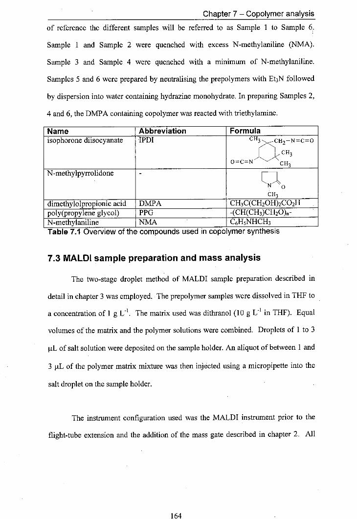
Chapter 7 - Copolymer analysis
of reference the different samples will be referred to as Sample 1 to Sample 6.
Sample 1 and Sample 2 were quenched with excess N-methylaniline (NMA).
Sample 3 and Sample 4 were quenched with a minimum of N-methylaniline.
Samples 5 and 6 were prepared by neutralising the prepolymers with Et3N followed
by dispersion into water containing hydrazine monohydrate. In preparing Samples 2,
4 and 6, the DMPA containing copolymer was reacted with triethylamine.
Name Abbreviation Formula isophorone diisocyanate IPDI CH3 U2—N=C=O
CH3
0 = C = N CH3
N-methylpyrrolidone
[7N'o
-
CH3
dimethylolpropionic acid DMPA CH3C(CH20H)2CO2H poly(propylene glycol) PPG -(CH(CH3)CH20)- N-methylaniline NMA C6H5NHCH3 Table 7.1 Overview 01 me compounas usea in copoiymer syninesis
7.3 MALDI sample preparation and mass analysis
The two-stage droplet method of MALDI sample preparation described in
detail in chapter 3 was employed. The prepolymer samples were dissolved in THF to
a concentration of 1 g U1. The matrix used was dithranol (10 g U' in THF). Equal
volumes of the matrix and the polymer solutions were combined. Droplets of 1 to 3
tL of salt solution were deposited on the sample holder. An aliquot of between 1 and
3 .tL of the polymer matrix mixture was then injected using a micropipette into the
salt droplet on the sample holder.
The instrument configuration used was the MALDI instrument prior to the
flight-tube extension and the addition of the mass gate described in chapter 2. All
164
Chapter 7 - Copolymer analysis
spectra were recorded in the reflectron mode. PEG standards were used for external
calibration.
7.4 Results.
7.4.1 Predicted products
The aim of the polymer preparation employed in the manufacture of Samples
1 to 4 was the production of polymers with the structures shown in table 7.2.
MALDI was used to determine whether the anticipated copolymers had been
synthesised. The results of the MALDI analysis will be discussed in three groups.
Samples produced under similar conditions will be grouped together. The first group
consists of Samples 1 and 2, the second group is made up of Samples 3 and 4 and the
final group discussed contains Samples 5 and 6.
The evaluation of the results will be qualitative i.e. attention will be confined
to the determination of the structure of the polymers present. Quantitative analysis,
e.g. average molecular weight determination and relative abundance of the various
polymer species present in each sample, was not attempted. The main reason for not
carrying out quantitative analysis was due to uncertainty over the ionisation
efficiency of the various polymer species present, as differences in ionisation
efficiency could lead to inaccurate relative abundance as well as inaccurate average
molecular weights. Another reason for not carrying out quantitative analysis is the
comparatively wide mass ranges of the polymers under investigation. MALDI has
been shown to give poor agreement with other techniques for average mass
determination of polydisperse polymer samples [4,5].
165
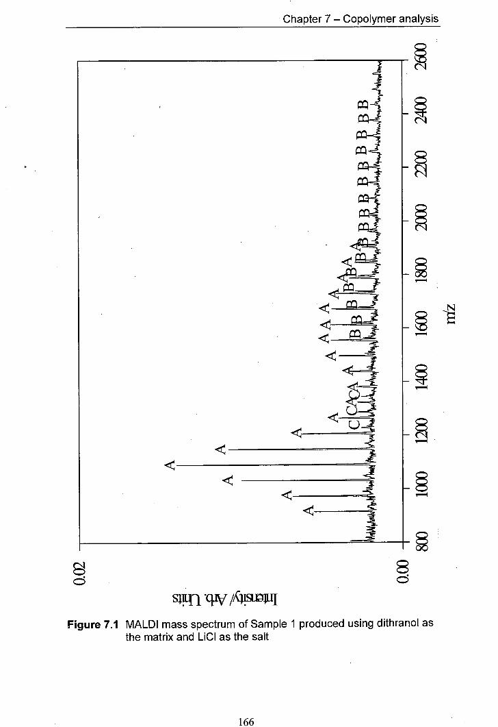
1
IT
11
Chapter 7 - Copolymer analysis
F=11 8 C5 C5
sum W 1ícuj
Figure 7.1 MALDI mass spectrum of Sample 1 produced using dithranol as the matrix and LiCI as the salt
166
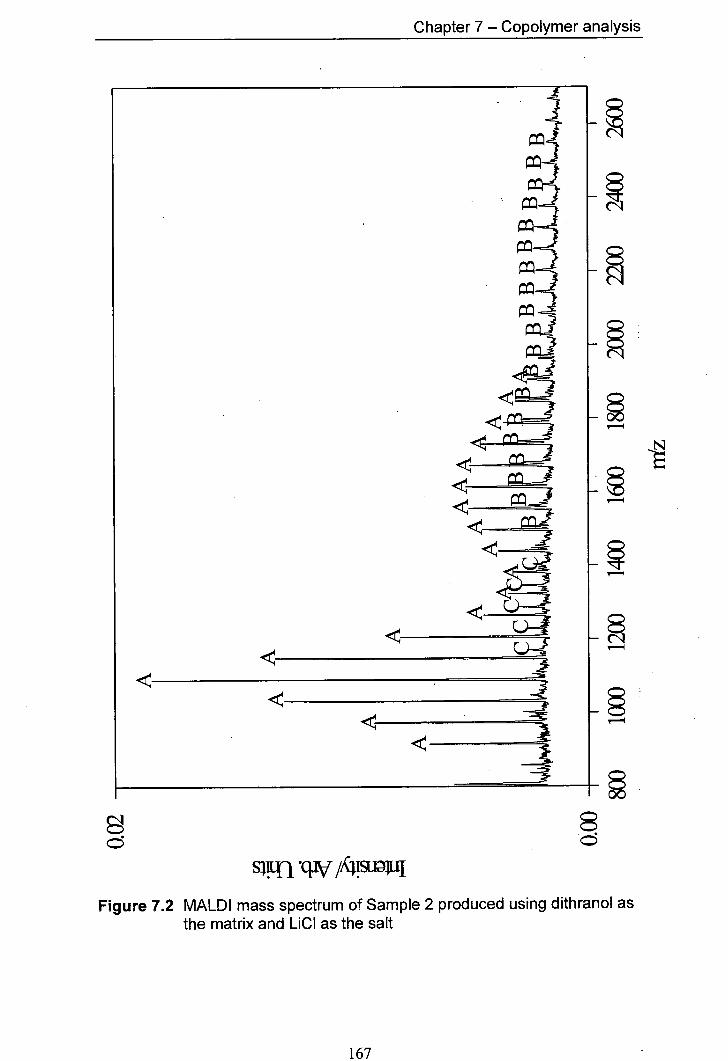
-J
il E-a
1-05,
Chapter 7 - Copolymer analysis
s1n cw /f4N1UJ
Figure 7.2 MALDI mass spectrum of Sample 2 produced using dithranol as the matrix and LiCI as the salt
167
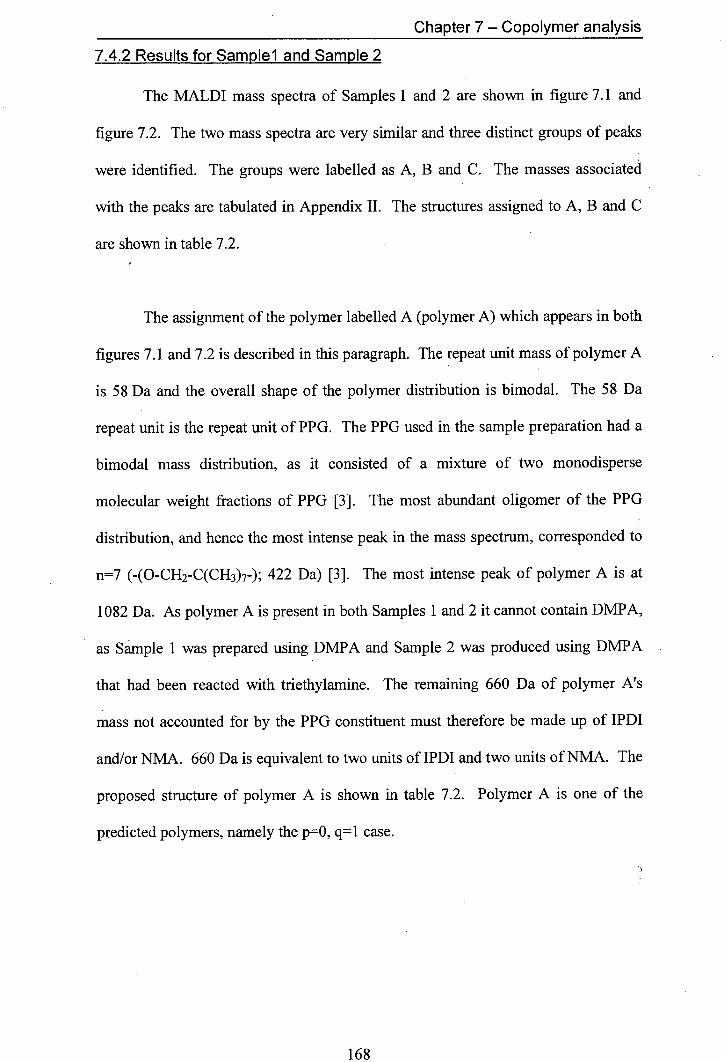
Chapter 7 - Copolymer analysis
7.4.2 Results for Sample I and Sample 2
The MALDI mass spectra of Samples 1 and 2 are shown in figure 7.1 and
figure 7.2. The two mass spectra are very similar and three distinct groups of peaks
were identified. The groups were labelled as A, B and C. The masses associated
with the peaks are tabulated in Appendix II. The structures assigned to A, B and C
are shown in table 7.2.
The assignment of the polymer labelled A (polymer A) which appears in both
figures 7.1 and 7.2 is described in this paragraph. The repeat unit mass of polymer A
is 58 Da and the overall shape of the polymer distribution is bimodal. The 58 Da
repeat unit is the repeat unit of PPG. The PPG used in the sample preparation had a
bimodal mass distribution, as it consisted of a mixture of two monodisperse
molecular weight fractions of PPG [3]. The most abundant oligomer of the PPG
distribution, and hence the most intense peak in the mass spectrum, corresponded to
n=7 (-(O-CH2-C(CH3)7-); 422 Da) [3]. The most intense peak of polymer A is at
1082 Da. As polymer A is present in both Samples 1 and 2 it cannot contain DMPA,
as Sample 1 was prepared using DMPA and Sample 2 was produced using DMPA
that had been reacted with triethylamine. The remaining 660 Da of polymer A's
mass not accounted for by the PPG constituent must therefore be made up of IPDI
and/or NMA. 660 Da is equivalent to two units of IPDI and two units of NMA. The
proposed structure of polymer A is shown in table 7.2. Polymer A is one of the
predicted polymers, namely the p=O, q=1 case.
168
Chapter 7 - Copolymer analysis
Polymer B is present in both Samples 1 and 2. The repeat unit is 58 Da and
the shape of the mass distribution appears to be bimodal; however, the mass
distribution is considerably wider than the mass distribution observed for polymer A.
The 58 Da repeat unit is PPG. The greater width of the mass distribution
suggests that this polymer contains two PPG units. The shape of the mass
distribution should then be trimodal. However, as the signal intensity decreases at
higher masses this is not actually observed. The most intense peak in the polymer B
distribution is seen where the sum of the number of PPG subunits is 14 i.e. both PPG
subunits are the 7mer or a combination of the 6mer and the 8mer etc. The mass of
the most intense polymer B peak is 1728 Da. The PPG constituents account for 844
Da of this mass. As with polymer A, the rest of the polymer is made up of IPDI and
NMA, in this case three IPDI units and 2 NMP units. Polymer B corresponds to the
predicted polymer (table 7.2) with p=O and q=2. Polymer B is shown in table 7.2.
Polymer C is only gives rise to a weak signal, with only five peaks of the
mass distribution having a sufficiently good signal to noise ratio to be
unambiguously recognisable (see figures 7.1 and 7.2). The most intense peak of the
polymer C distribution has a mass of 1278 Da. Polymer C is 196 Da heavier than
Polymer A. Isocyanates are known to form dimers in the presence of water with the
loss of CO (see figure 7.3) [6]. The mass of IPDI that has lost CO is 196 Da. The
most probable structure for polymer C, therefore, is analogous to polymer A, with
one of the diisocyanates replaced by the diisocyanate dimer. The proposed structure
of polymer C is given in table 7.2.
169
Chapter 7 - Copolymer analysis
RNC0 + H 2 0 No [R —NH __C__0H1 . R—NH+ CO2
RNCO
R—NH--C—NH—R
0 Figure 7.3 Dimer formation in isocyanates
The analysis of Samples 1 and 2 by MALDI MS confirms that two of the
copolymers predicted from the synthesis are produced, namely the p=O, q=l and the
p=O, q=2 possibilities. The presence of a by-product due to dimerisation of the
diisocyanate was also observed. DMPA is not incorporated into any of the
copolymers detected.
7.4.3 Results for Sample 3 and Sample 4
Samples 3 and 4 gave very similar mass spectra (figures 7.4 and 7.5). In the
mass spectra for both samples three polymer distributions could be distinguished,
labelled as A, D and E. The fact that the same species were found in Samples 3 and
4 indicates that as with Samples 1 and 2, DMPA-containing polymers were not
detected.
All the three polymer distributions have a very similar overall shape.
Polymer A is the same as polymer A in figures 7.1 and 7.2. The differences in mass
170

Structure Comments
0
I I
0 0
NHJ Ph
general structure
N
Ph(N
NH H -
--"
0 01 MOOC
jll~, j
NH NH10NH
[il- n 0 0
M = H or NEt 4- —q 2
0
Ph A
Polymer A
N
0 r
Polymer B
Ph N NH
NH NHJ
Y
NHNPh
-
0 0
—2
_N NH &NHi oNH&NH
__ _
[0
Polymer C
Ph N H
0 n
yPh N H
0 0
Table 7.2 Summary of the structures of the polymers found in Sample I and Sample 2
Cl)
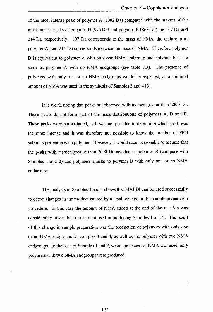
Chapter 7 - Copolymer analysis
of the most intense peak of polymer A (1082 Da) compared with the masses of the
most intense peaks of polymer D (975 Da) and polymer E (868 Da) are 107 Da and
214 Da, respectively. 107 Da corresponds to the mass of NMA, the endgroup of
polymer A, and 214 Da corresponds to twice the mass of NMA. Therefore polymer
D is equivalent to polymer A with only one NMA endgroup and polymer E is the
same as polymer A with no NMA endgroups (see table 7.3). The presence of
polymers with only one or no NMA endgroups would be expected, as a minimal
amount of NMA was used in the synthesis of Samples 3 and 4 [3].
It is worth noting that peaks are observed with masses greater than 2000 Da.
These peaks do not form part of the mass distributions of polymers A, D and E.
These peaks were not assigned, as it was not possible to determine which peak was
the most intense and it was therefore not possible to know the number of PPG
subunits present in each polymer. However, it would seem reasonable to assume that
the peaks with masses greater than 2000 Da are due to polymer B (compare with
Samples 1 and 2) and polymers similar to polymer B with only one or no NMA
endgroups.
The analysis of Samples 3 and 4 shows that MALDI can be used successfully
to detect changes in the product caused by a small change in the sample preparation
procedure. In this case the amount of NMA added at the end of the reaction was
considerably lower than the amount used in producing Samples 1 and 2. The result
of this change in sample preparation was the production of polymers with only one
or no NMA endgroups for samples 3 and 4, as well as the polymer with two NMA
endgroups. In the case of Samples 1 and 2, where an excess of NMA was used, only
polymers with two NMA endgroups were produced.
172
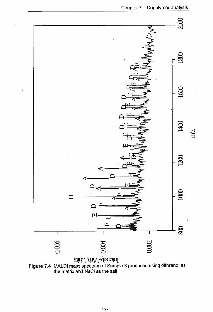
II
Chapter 7 - Copolymer analysis
§ 9 9 C:5 C5 C5
S11n 41\/ /Jc4!L1J Figure 7.4 MALDI mass spectrum of Sample 3 produced using dithranol as
the matrix and NaCI as the salt
173
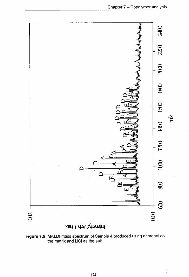
J ~z
OF
-J
S11fl t
Chapter 7 —Copolymer analysis
Figure 7.5 MALDI mass spectrum of Sample 4 produced using dithranol as the matrix and LiCI as the salt
174
Chapter 7 - Copolymer analysi
o_ 00
EE E> -CL
a :i5 E - >'
uJ
E 0 11
CL
)—o I
0 H 0 II 0
H 0
o 'C
0
0 'C
I
0
'C
0
=
0
=
I
C.)
Cl)
/ o< \ z—
a-
0-K z—
CL
z
0
0
175
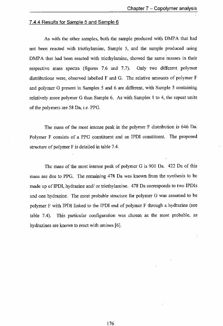
Chapter 7 - Copolymer analysis
7.4.4 Results for Sample 5 and Sample 6
As with the other samples, both the sample produced with DMPA that had
not been reacted with triethylamine, Sample 5, and the sample produced using
DMPA that had been reacted with triethylamine, showed the same masses in their
respective mass spectra (figures 7.6 and 7.7). Only two different polymer
distributions were, observed labelled F and G. The relative amounts of polymer F
and polymer G present in Samples 5 and 6 are different, with Sample 5 containing
relatively more polymer G than Sample 6. As with Samples 1 to 4, the repeat units
of the polymers are 58 Da, i.e. PPG.
The mass of the most intense peak in the polymer F distribution is 646 Da.
Polymer F consists of a PPG constituent and an IPDI constituent. The proposed
structure of polymer F is detailed in table 7.4.
The mass of the most intense peak of polymer G is 900 Da. 422 Da of this
mass are due to PPG. The remaining 478 Da was known from the synthesis to be
made up of IPDI, hydrazine and/ or triethylamine. 478 Da corresponds to two IPDIs
and one hydrazine. The most probable structure for polymer G was assumed to be
polymer F with IPDI linked to the IPDI end of polymer F through a hydrazine (see
table 7.4). This particular configuration was chosen as the most probable, as
hydrazines are known to react with amines [6].
176
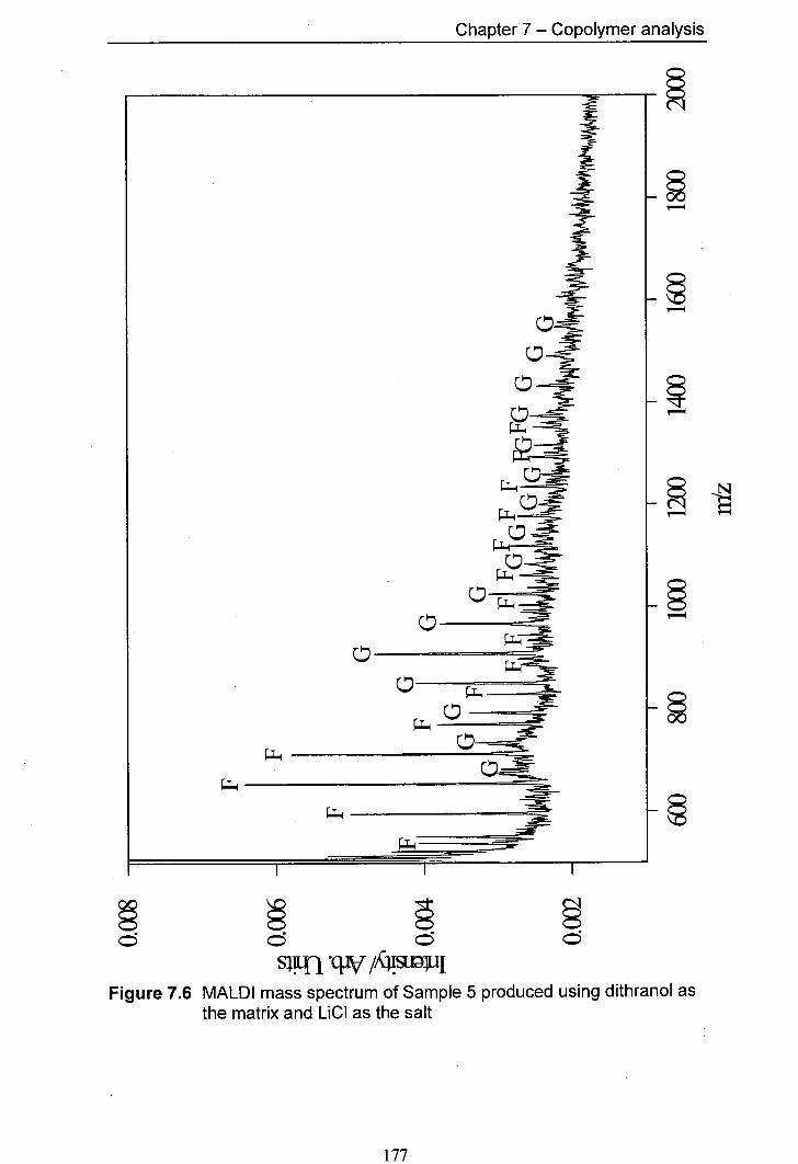
IIA
0
ME
I:
00i
Chapter 7 - Copolymer analysis
§ § 9 9 S1M1 •qJ ,ciiuj
Figure 7.6 MALDI mass spectrum of Sample 5 produced using dithranol as the matrix and LiCI as the salt
177
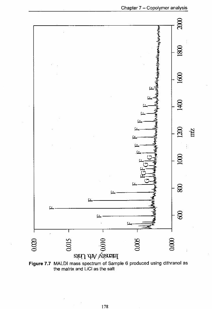
-J -J [I
0
-J
nn
01~
Chapter 7 - Copolymer analysis
SLfl t /11!L1I Figure 7.7 MALDI mass spectrum of Sample 6 produced using dithranol as
the matrix and L1CI as the salt
178
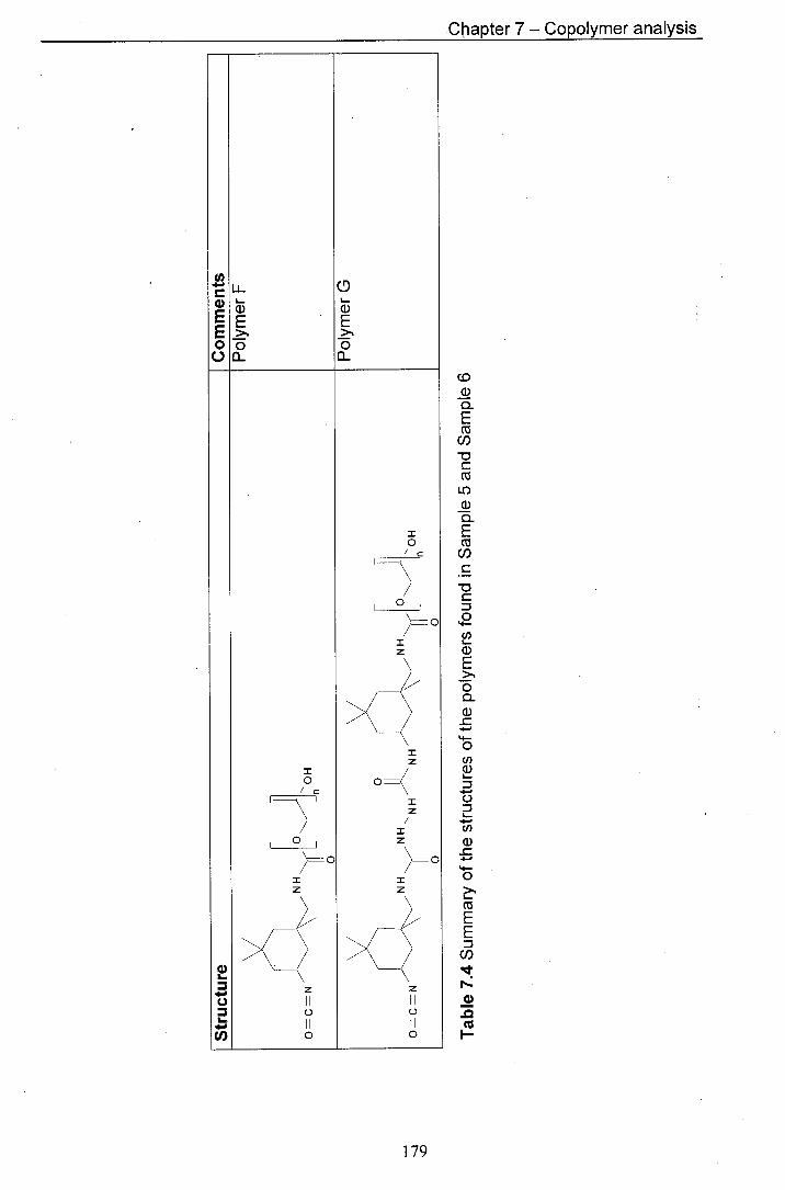
Chapter 7 - Copolymer analysis
OQ_
E2:1 00
(9
E 0
I 0
I
= or
I Z
I z I
0 0
C.) z II
z II
— 0 II
0
CD a)
CL Ct
C/)
cu LC) a) CL- E (ti U) C
C
10 C/) a) E > 0 a. (D -I-.
4- 0 Cl) a)
0
U) a) 4- 0
E E
CO 14 —a) -Q F-
-
179
Chapter 7 - Copolymer analysis
7.5 Conclusions
The results described in this chapter show that MALDI can be a very
powerful tool for copolymer analysis. It was possible to determine a large amount of
information on the structure of the polymers under investigation using only the
MALDI mass spectra obtained and information on the sample preparation. The
structural information obtained included repeat unit masses and endgroup
information, from samples consisting of more than one polymer. The analysis was
limited to qualitative evaluation, as the relative ionisation efficiencies of the different
polymers are not known.
The appearance of new polymer species due to changes in the reaction
conditions during polymer synthesis was readily detected. This was best illustrated
by comparing two polymer samples, one of which had been produced using an
excess of N-methylaniline (NMA), and the other with a minimal amount of NMA.
All polymers produced in the presence of excess NMA had two NMA endgroups,
whereas the polymers produced using minimal NMA had a range of different
numbers of NMA endgroups.
Chapter 7 - Copolymer analysis
7.6 References
S. Yoshida, S. Yamoto and T. Takamatsu, Rapid Commun. Mass Spectrom., 9, 535-544 (1998) V.. Schädler, J. Spickermann, H. J. Rader and U. Wiesner, Macromolecules, 29, 4865-4870 (1996) Private correspondence with manufacturer (1995) J. Axeisson, E. Scrivener, D. M. Haddleton and P. J. Derrick, Macromolecules, 29, 8875-8882 (1996) K. Martin, J. Spickermann, H. J. Rader and K. Mullen, Rapid Commun. Mass Spectrom., 10, 1471-1474 (1996) R. T. Morrison and R. N. Boyd, 'Organic Chemistry', Fifth Edition, Allyn and Bacon, Inc., Newton, Massachusetts 02159, USA
181
Chapter 8 - Conclusions and further work
Chapter 8— Conclusions and further work
8.1 Introduction
Matrix Assisted Laser Desorptionllonisation (MALDI) time-of-flight mass
spectrometry has been shown to have great potential as a technique for synthetic
polymer mass analysis. It was the aim of this research to build on and extend
previous work on the mass spectrometric analysis of synthetic polymers carried out
at the University of Edinburgh.
The studies carried out can be divided into two broad categories. The first
category concerns the practical aspects of polymer analysis by MALDI; here the
issues of improving sample preparation, extending the high-mass capability of the
mass spectrometer and the study of novel synthetic polymers were addressed. The
second group of studies dealt with more fundamental issues affecting polymer mass
analysis by MALDI. For this work a study of post source decay of synthetic
polymers was made and delayed extraction experiments were carried out.
182
Chapter 8 - Conclusions and further work
8.2 Practical development of MALDI mass spectrometry for
synthetic polymers
Sample preparation improvements were made in two ways. First, a more
reproducible sample preparation method was developed in order to be able to carry
out high quality quantitative studies. The technique developed to this end was an
aerosol sample deposition technique. Secondly, the range of matrices and matrix to
analyte ratios used in sample preparation was reviewed and extended which led to
great improvements in high-mass detection.
In order to detect high-mass polymers effectively the mass spectrometer was
upgraded by the addition of a mass gate. This is a gated deflection plate, which was
used to deflect low-mass ions that would otherwise have lead to detector saturation.
Through instrument modification and improved sample preparation, it was possible
to detect polymers with average molecular weights of 20000 Da. Dimers of these
polymers were also detected with masses in excess of 40000 Da. The previous upper
detection limit for the Edinburgh instrument was ca 10000 Da.
During the course of this work numerous novel polymers were analysed using
MALDI. These studies illustrated the capacity of MALDI mass spectrometry to
yield detailed information on end-group and repeat unit masses of copolymers.
183
Chapter 8 - Conclusions and further work
8.3 Studies of the MALDI process
Two studies were conducted to investigate the ionisation process and post
source decay respectively.
In the ionisation study use was made of delayed extraction. In these
experiments the improvements in quantification afforded by the aerosol sample
preparation technique, which had been developed previously, were exploited. The
most notable result obtained from this work was the observation that metal ion
adduct yields did not increase by allowing a time delay between the laser shot and
ion extraction. Previously reported work suggested otherwise. The present work is
interpreted as evidence against the often-suggested gas-phase ion attachment process
and lends weight to a 'prompt' ionisation process.
Post source decay experiments were carried out. These experiments showed
a clear correlation between the size of alkali metal ions attached to polymers and the
extent to which these polymer metal ion adducts dissociated. Rb and, to a lesser
extent, K adducts of a range of polymers underwent post source decay, but Li and
Na adducts of the same polymers did not decay.
8.4 Results not included
Several pieces of work were carried out that have not been included. One
such project was the mass analysis of industrial copolymer samples, which could not
be reported on for confidentiality reasons. A series of experiments was carried out
184
Chapter 8 - Conclusions and further work
on the 'matrix-suppression' effect The results of these experiments were not
deemed to be of high enough quality to be included in this thesis. Also several
peptides were mass analysed. The biomolecule work was primarily done to test the
high-mass capability of the instrument, work that was repeated using synthetic
polymers.
8.5 Future work
In the light of research completed to date several further experiments can be
suggested.
The aerosol sample preparation technique would lend itself to coupling with
liquid chromatography separation. It may be possible to couple this sample
deposition method directly to the source of a mass spectrometer, leading to an
automated interface.
The dynamics of post source decay could be further investigated by means of
a movable deflection plate within the flight tube of the mass spectrometer.
Improvements in high-mass detection could be brought about by redesigning
the source region of the mass spectrometer to make high-voltage delayed extraction
possible. It would also be desirable to move to a detection system that is more
sensitive to slow heavy ions than the traditional microchannel plate detector.
185

Chapter 8 - Conclusions and further work
Finally, it would be interesting to investigate the use of different laser
systems such as femtosecond lasers for MALDI.
186
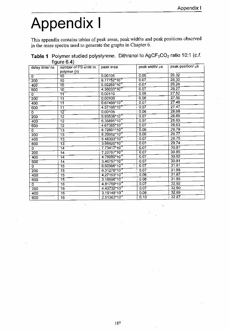
Appendix I
Appendix I This appendix contains tables of peak areas, peak widths and peak positions observed in the mass spectra used to generate the graphs in Chapter 6.
Table I Polymer studied polystyrene. Dithranol to AgCF3CO2 ratio 10:1 (c. f. fiaure 6.4)
delay time/ ns number of PS units in polymer(
peak area peak width/ is peak position! is
o 10 0.00105 0.06 26.32
200 10 9.77752*10 0.07 26.30
400 10 6.02265*10 0.07 26.28
600 10 4.36033*10 0.07 26.27
0 11 0.00110 0.06 27.52
200 11 0.00100 0.06 27.50
400 11 6.67466*10 0.07 27.48
600 11 4.57166*10 0.07 27.47
0 12 0.00105 0.06 28.68
200 12 9.93638*10 0.07 28.65
400 12 6.35895*10 0.07 28.63
600 12 4.67385*10 0.07 28.63
0 13 8.72601 *10-" 0.06 29.79
200 13 8.20662*10 0.06 29.77
400 13 5.48303*10 0.07 29.75
600 13 3.98620*10 =4 0.07 29.74
0 14 7.73417*10 0.07 30.87
200 14 7.20767*10 0.07 30.85
400 14 4.78089*10 0.07 30.82
600 14 3.46757*10 0.07 30.81
0 15 6.60998*10 0.07 31.91
200 15 6.31276*10 0.07 31.88 400 15 4.27153*10 =4 0.08 31.87
600 15 3.18898*10-4 0.08 31.85
0 16 4.81759*10 0.07 32.92 200 16 4.43732*10* 0.07 32.90
400 16 3.19148*10 0.08 32.89 600 16 2.51303*10 0.10 32.87
187
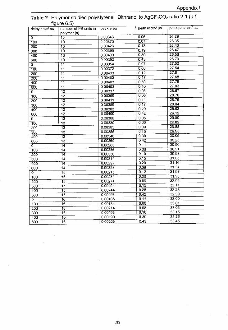
Appendix I
Table 2 Polymer studied polystyrene. Dithranol to AgCF3CO2 ratio 2:1 (C.f fiaure6.5'
delay time/ ns number of PS units in polymer (n)
peak area peak width/ ts peak position! lis
o 10 0.00346 0.06 26.29
100 10 0.00370 0.07 26.35
200 10 0.00426 0.13 26.40
300 10 0.00395 0.19 26.47
400 10 0.00403 0.30 26.56
600 10 0.00392 0.43 26.70
0 11 0.00354 0.07 27.50
100 11 0.00372 0.06 27.54
200 11 0.00433 0.12 27.61
300 11 0.00403 0.17 27.68
400 11 0.00403 0.30 27.78
600 11 0.00403 0.40 27.93
0 12 0.00337 0.08 28.67
100 12 0.00359 0.06 28.70
200 12 0.00411 0.11 28.76
300 12 0.00389 0.17 28.84
400 12 0.00383 0.29 28.92
600 12 0.00400 0.42 29.12
0 13 0.00308 0.08 29.80
100 13 0.00330 0.06 29.82
200 13 0.00383 0.09 29.88
300 13 0.00355 0.15 29.95
400 13 0.00346 0.30 30.05
600 13 0.00365 0.42 30.23
0 14 0.00265 0.11 30.90
100 14 0.00286 0.06 30.91
200 14 0.00336 0.10 30.98
300 14 0.00314 0.15 31.05
400 14 0.00297 0.29 31.16
600 14 0.00323 0.39 31.31
0 15 0.00215 0.12 31.97
100 15 0.00234 0.06 31.98
200 15 0.00274 0.09 32.05
300 15 0.00254 0.15 32.11
400 15 0.00244 0.28 32.23
600 15 0.00263 0.42 32.39
0 16 0.00165 0.11 33.00
100 . 16 0.00184 0.06 33.01
200 16 0.00214 0.08 33.08 300 16 0.00198 0.16 33.15
400 16 0.00190 0.30 33.25 600 16 0.00205 0.43 33.45
188

Appendix I
Table 3 Polymer studied polystyrene. Dithranol to AgCF3CO2 ratio 1:1 (c.f. flaure 6.6'
delay time/ ns number of PS units in polymer (n)
peak area peak width! .ts peak position! is
o 10 0.00433 0.05 26.29 100 10 0.00366 0.08 26.35 200 10 0.00349 0.14 26.40
300 10 0.00268 0.19 26.46 400 10 0.00234 0.29 26.56
600 10 0.00199 0.39 26.68
0 11 0.00406 0.06 27.49
100 11 0.00354 0.07 27.54
200 11 0.00320 0.13 27.62
300 11 0.00249 0.19 27.67 400 11 0.00232 0.29 27.81 600 11 0.00193 0.40 27.93
0 12 0.00348 0.07 28.65
100 12 0.00322 0.06 28.69 200 12 0.00281 0.13 28.76 300 12 0.00223 0.20 28.83
400 12 0.00211 0.30 28.92 600 12 0.00173 0.41 29.08
0 13 0.00317 0.08 29.77
100 13 0.00290 0.06 29.80
200 13 0.00252 0.13 29.87
300 13 0.00199 0.21 29.96 400 13 0.00191 0.33 30.06 600 13 0.00159 0.42 30.21 0 14 0.00248 0.08 30.85 100 14 0.00238 0.06 30.89 200 14 0.00204 0.10 30.97 300 14 0.00159 0.20 31.04 400 14 0.00155 0.31 31.17 600 14 0.00127 0.37 31.28 0 15 0.00204 0.11 31.94 100 15 0.00192 0.06 31.95 200 15 0.00164 0.11 32.02 300 15 0.00128 0.19 32.08 400 15 0.00124 0.35 32.23 600 15 0.00107 0.40 32.36 0 16 0.00148 0.10 32.97 100 16 0.00143 0.05 32.98 200 16 0.00120 0.09 33.05 300 16 9.18276*10 0.18 33.13 400 16 8.84717*10 0.27 33.20 600 16 1 7.28138*10 0.42 33.33
189
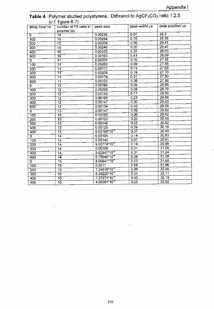
Appendix
Table 4 Polymer studied polystyrene. Dithranol to AgCF3CO2 ratio 1:2.5 (r f firiur A7
delay time/ ns number of PS units in polymer (n)
peak area peak width/ p.s peak position! p.s
o 10 0.00238 0.07 26.3
100 10 0.00294 0.10 26.36
200 10 0.00209 0.16 26.41
300 10 0.00246 0.20 26.47
400 10 0.00205 0.32 26.63
600 10 0.00163 0.41 26.69
0 11 0.00201 0.10 27.52
100 11 0.00260 0.09 27.56
200 11 0.00177 0.15 27.62
300 11 0.00206 0.19 27.70
400 11 0.00174 0.31 27.80
600 11 0.00132 0.36 27.99
0 12 0.00166 0.09 28.69
100 12 0.00209 0.08 28.70
200 12 0.00143 0.17 28.80
300 12 0.00168 0.23 28.88
400 12 0.00147 0.30 28.93
600 12 0.00104 0.43 29.06
0 13 0.00147 0.09 29.82
100 13 0.00185 0.06 29.82
200 13 0.00123 0.20 29.90
300 13 0.00146 0.25 30.02
400 13 0.00125 0.39 30.18
600 13 9.03796*10 0.37 30.40
0 14 0.00104 0.14 30.93
100 14 0.00142 0.07 30.91
200 14 9.00774*10 0.14 30.98
300 14 0.00108 0.31 31.08
400 14 9.92947*10 =4 0.31 31.24
600 14 6.75848*10 0.26 31.35
0 15 8.00941 *10-" 0.13 31.99
100 15 0.0011 0.06 31.96
200 15 7.24616*10 0.09 32.05
300 15 8.39225*10 0.21 32.11
400 15 7.37971 *10-4 0.45 32.19
600 15 4.66581*10 0.25 32.52
190
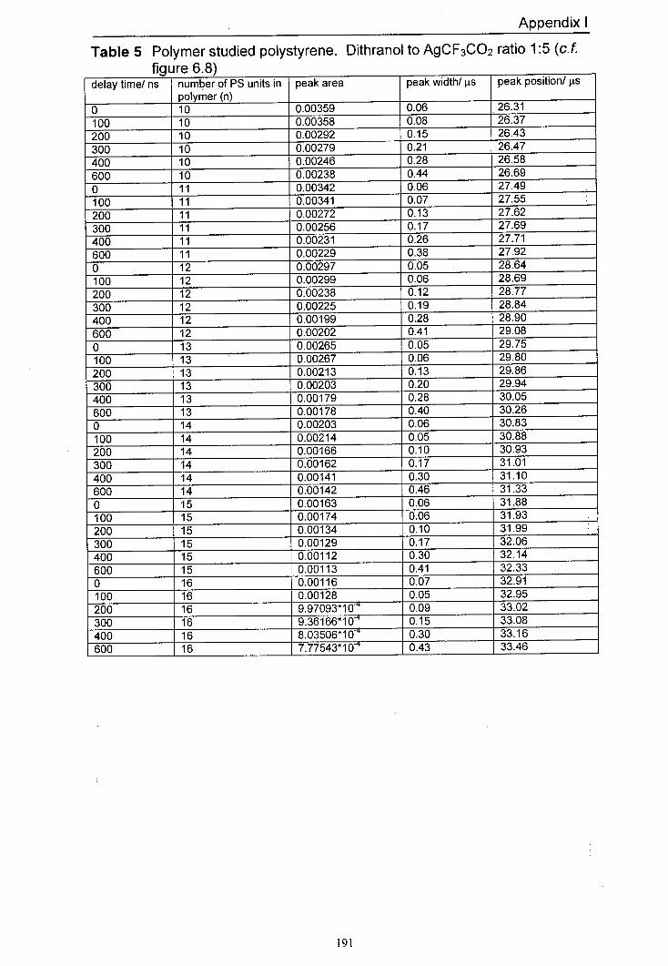
Appendix I
Table 5 Polymer studied polystyrene. Dithranol to AgCF3CO2 ratio 1:5 (Cf finiir A R'
delay time/ ns number of PS units in polymer (n)
peak area peak width/ j.ts peak position! ts
o 10 0.00359 0.06 26.31
100 10 0.00358 0.08 26.37
200 10 0.00292 0.15 26.43
300 10 0.00279 0.21 26.47
400 10 0.00246 0.28 26.58
600 10 0.00238 0.44 26.69
0 11 0.00342 0.06 27.49
100 11 0.00341 0.07 27.55
200 11 0.00272 0.13 27.62
300 11 0.00256 0.17 27.69
400 11 0.00231 0.26 27.71
600 11 0.00229 0.38 27.92
0 12 0.00297 0.05 28.64
100 12 0.00299 0.06 28.69
200 12 0.00238 0.12 28.77
300 12 0.00225 0.19 28.84
400 12 0.00199 0.28 28.90
600 12 0.00202 0.41 29.08
0 13 0.00265 0.05 29.75
100 13 0.00267 0.06 29.80
200 13 0.00213 0.13 29.86
300 13 0.00203 0.20 29.94
400 13 0.00179 0.28 30.05
600 13 0.00178 0.40 30.26
0 14 0.00203 0.06 30.83
100 14 0.00214 0.05 30.88
200 14 0.00166 0.10 30.93
300 14 0.00162 0.17 31.01
400 14 0.00141 0.30 31.10
600 14 0.00142 0.46 31.33
0 15 0.00163 0.06 31.88
100 15 0.00174 0.06 31.93
200 15 0.00134 0.10 31.99
300 15 0.00129 0.17 32.06
400 15 0.00112 0.30 32.14
600 15 0.00113 0.41 32.33
0 16 0.00116 0.07 32.91
100 16 0.00128 0.05 32.95 200 16 9.97093*10 4 0.09 33.02
300 16 9.36166*10 0.15 33.08
400 16 8.03506*10 0.30 33.16 600 16 7.77543*10 0.43 33.46
191

Appendix I
Table 6 Polymer studied PMMA. Dithranol to LiCI ratio 1:1 (cf figure 6.10) delay time/ ns number of PMMA
units in polymer (n) peak area peak width/ lts peak position! ts
o 9 4739*10 1 0.07 30.35
100 9 3.587*10-4 0.05 30.32
200 9 3.273*10 0.06 30.31
300 9 3.584*10 0.06 30.30
400 9 4.115*10 0.07 30.29
0 10 4.982*10 0.07 31.97
100 10 4.379*10 0.05 31.94
200 10 3.772*10 0.06 31.93
300 10 3.675*10 0.05 31.92
400 10 4.270*10 0.06 31.92
0 11 5.488*10 0.06 33.52
100 11 4.716*10 0.05 33.49
200 11 4.368*10 0.06 33.48
300 11 4.221 *10-4 0.06 33.47
400 11 4.605*10 4 0.06 33.46
0 12 5.599*10 0.06 35.00
100 12 5.015*101 0.05 34.97
200 12 4.769*10 0.05 34.96
300 12 4.410*10 0.05 34.95
400 12 4.702*10 0.06 34.94
0 13 6.123*10 0.06 36.41
100 13 5.539*10 0.05 36.38 200 13 5.209*10 0.06 36.37
300 13 4.862*10 0.06 36.37
400 13 5.015*10 0.06 36.36 0 14 6.271*10 0.06 37.78
100 14 6.052*10-4 0.05 37.75 200 14 5.542*10 0.06 37.74 300 14 5.114*10 0.05 37.73
400 14 5.403*10 0.07 37.72 0 15 6.197*10 0.06 39.09
100 15 5.783*10 0.05 39.06 200 15 5.391*10 0.05 39.05 300 15 5.342*10* 0.06 39.04 400 15 5.408*10 0.06 39.03 0 16 5.561*10 0.06 40.36 100 16 5.446*10 0.05 40.33 200 16 5.443*10 0.06 40.32 300 16 4.560*10 0.06 40.31 400 16 4.897*10 0.07 40.30 0 17 4.934*10 0.06 41.59 100 17 5.064*10 0.06 41.56 200 17 4579*10* 0.06 41.55 300 17 4.136*10 0.06 41.54 400 17 4.226*10 0.07 41.53 0 18 4.765*10 0.07 42.79 100 18 4.501*10 0.05 42.76 200 18 4.028*10 0.06 42.75 300 18 3.759*10 0.07 42.74 400 18 3.917*10 0.07 42.73 0 19 4.401 *10-4 0.07 43.95 100 19 4.240*10 0.06 43.92 200 19 3.696*10 0.06 43.91 300 19 3.647*10 0.07 43.90 400 19 3.620*10 =4 0.07 43.90 0 20 3.922*10 0.08 45.08 100 20 3.298*10 0.06 45.06 200 20 3.240*10 0.07 45.05
192
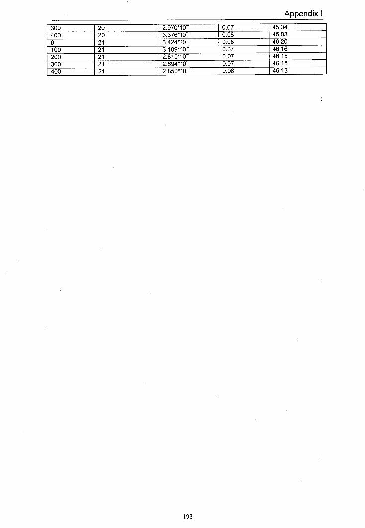
Appendix U
300 20 2.970*10 0.07 45.04 400 20 3.376*10-4 0.08 45.03 0 21 3.424*10 0.08 46.20 100 21 3.109*10 0.07 46.16 200 21 2.810*10 0.07 46.15 300 21 1 2.694*10 0.07 46.15 400 21 1 2.850*10 0.08 46.13
193
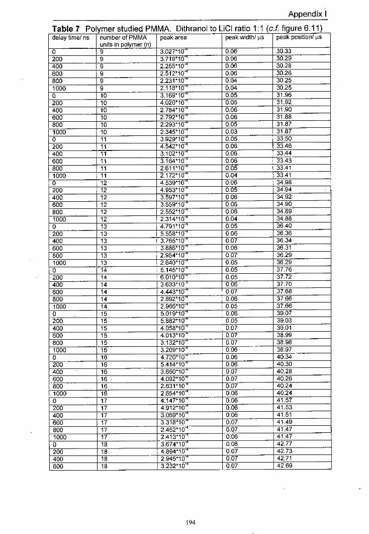
Appendix I
Table 7 Polymer studied PMMA. Dithranol to LICI ratio 1:1 (ci. fiqure 6.11) delay time/ ns - number of PMMA
units in polymer (n) peak area peak width/ ts peak position/ jAs
o 9 3.027*10 0.06 30.33 200 9 3.719*10 0.06 30.29 400 9 2.255*10 0.06 30.28 600 9 2512*10.4 0.06 30.26 800 9 2.231*10 0.04 30.25 1000 9 2.118*10 0.04 30.25 0 10 3.169*10 0.05 31.96 200 10 4.020*10 0.05 31.92 400 10 2.784*10 0.06 31.90 600 10 2.792*10 0.06 31.88 800 10 2.293*10 0.05 31.87 1000 10 2.345*10 0.03 31.87 0 11 3.929*10 0.05 33.50 200 11 4.542*10 0.06 33.46 400 11 3.102*10 0.06 33.44 600 11 3.164*10 0.06 33.43 800 11 2.611*10 0.05 33.41 1000 11 2.172*10 0.04 33.41 0 12 4.539*10 0.06 34.98 200 12 4.953*10 0.05 34.94 400 12 3.597*10 0.06 34.92 600 12 3.559*10 4 0.06 34.90 800 12 2.552*10 0.06 34.89 1000 12 2.314*10 4 0.04 34.88 0 13 4.791*10 0.05 36.40 200 13 5.558*10.4 0.06 36.36 400 13 3.765*10 0.07 36.34 600 13 3.886*10 0.06 36.31 800 13 2.954*10.4 0.07 36.29 1000 13 2.640*10 0.05 36.29 0 14 5.145*10 0.05 37.76 200 14 6.010*10+ 0.05 37.72 400 14 3.633*10 0.06 37.70 600 14 4.443*10* 0.07 37.68 800 14 2.892*10' 0.06 37.66 1000 14 2.966*10 0.05 37.66 0 15 5.019*101 0.06 39.07 200 15 5.882*10-4 0.05 39.03 400 15 4.058*10 0.07 39.01 600 15 4.013*10 0.07 38.99 800 15 3.132*10 0.07 38.98 1000 15 3.209*10 0.06 38.97 0 16 4.720*10 0.06 40.34 200 16 5.414*10 0.06 40.30 400 16 3.650*10 0.07 40.28 600 16 4.092*10 0.07 40.26 800 16 2.631*10 0.07 40.24 1000 16 2.654*10 0.06 40.24 0 17 4.147*10 0.06 41.57 200 17 4.912*10* 0.06 41.53 400 17 3.069*10 0.06 41.51 600 17 3.318*10 0.07 41.49 800 17 2.452*10 0.07 41.47 1000 17 2.413*10 0.06 41.47 0 18 3.674*10 0.06 42.77 200 18 4.894*10 0.07 42.73 400 18 2.945*10 0.07 42.71 600 18 3.232*10 0.07 42.69
194
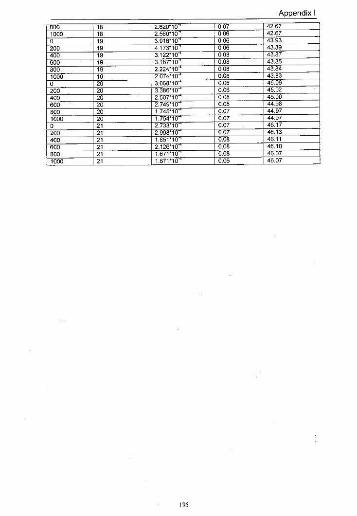
Appendix I
800 18 2.620*10 0.07 42.67 1000 18 2.560*10 0.06 42.67 0 19 3.916*10 0.06 43.93 200 19 4.173*10 0.06 43.89 400 19 3.122*10 0.08 43.87 600 19 3.187*10 0.08 43.85 800 19 2.224*10 0.08 43.84 1000 19 2.074*10 0.06 43.83 0 20 3.068*10 0.06 45.06 200 20 3.386*10 0.06 45.02 400 20 2.507*10 0.08 45.00 600 20 2.749*10* 0.08 44.98 800 20 1.745*10 0.07 44.97 1000 20 1.754*10 m 0.07 44.97 0 21 2TRj79-ol 0.07 46.17 200 21 2.998*10 0.07 46.13 400 21 1.851*10 0.08 t 46.11 600 21 2.126*10 0.08 46.10 800 21 1.671 *10-4 0.08 46.07 1000 21 1.671*10 0.06 46.07
195

Appendix I
Table 8 Polymer studied PEG. Dithranol to NaCI ratio 1:1 (c.f. figure 6.12) delay time/ ns number of PEG
units in polymer (n) peak area peak width/ ts peak position! j.ts
0 32 1.42337*10 0.06 38.31
100 32 1.65039*10' 0.06 38.29
200 32 1.51174*1O 0.06 38.26
300 32 1.66117*10 0.07 38.26
400 32 1.49362*10 0.08 38.25
0 34 2.09827*10 0.05 39.45
100 34 2.27745*10 0.05 39.43
200 34 2.25684*10 0.07 39.41
300 34 1.83101*10 0.07 39.40
400 34 2.01258*10 0.07 39.39
0 36 3.17611*10 0.06 40.56
100 36 3.34026*10 0.05 40.54
200 36 3.48645*10 0.07 40.52
300 36 3.11534*10 0.06 40.51
400 36 2.85967*10 0.07 40.50
0 38 4.08681*10 0.06 41.64
100 38 4.39870*10 0.05 41.62
200 38 4.58787*10 0.05 41.60
300 38 4.11218*10 0.06 41.60
400 38 3.87986*10 0.07 41.58
0 40 5.14006*10 0.06 42.70
100 40 5.61738*10 0.05 42.67
200 40 5.53812*10 0.06 42.65
300 40 5.10998*10 0.07 42.65
400 40 4.52991*10 0.07 42.64
0 42 5.63116*10 0.06 43.72 100 42 6.04627*10 0.06 43.70
200 42 5.80073*10 0.07 43.68 300 42 5.33777*10 0.06 43.67 400 42 4.98389*10 0.08 43.66
0 44 5.32025*10 0.06 44.72 100 44 5.74025*10 0.05 44.70 200 44 5.55283*10 0.07 44.68 300 44 5.29336*10 0.07 44.68 400 44 4.85034*10 0.07 44.67 0 46 4.98155*10 0.07 45.70 100 46 5.39914*10 0.06 45.68 200 46 5.40656*10 0.07 45.66 300 46 4.96495*10 1 0.07 45.66 400 46 4.35700*10 0.07 45.65 0 48 4.31516*10 0.07 46.66 100 48 4.47498*10 0.07 46.64 200 48 4.48801*10 0.07 46.62 300 48 4.08707*10 0.07 46.61 400 48 3.91414*10 0.08 46.61 0 50 3.84292*104 0.09 47.61 100 50 3.78803*10-' 0.07 47.58 200 50 3.74816*10 0.09 47.55 300 50 3.27501 *10 0.09 47.56 400 50 3.25947*10 0.09 47.55 0 52 3.28731*10 0.11 48.53 100 52 3.10892*10 0.08 48.51 200 52 3.53935*10 0.12 48.49 300 52 2.95685*10 0.10 48.47 400 52 1 2.93747*10 0.11 48.47
196
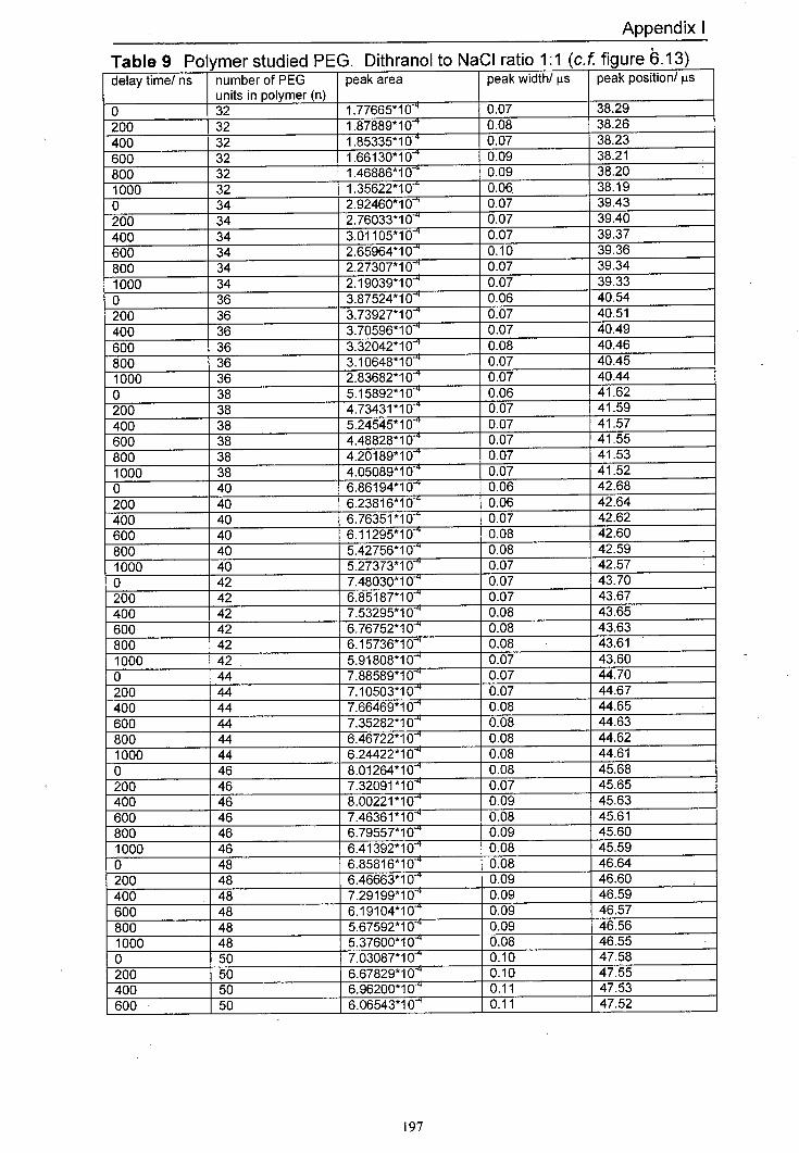
Appendix I
Table 9 Polymer studied PEG. Dithranol to NaCI ratio 1:1 (ci. figure .13) delay time/ ns number of PEG
units in polymer (n) peak area peak width/ lts peak position/ ts
o 32 1.77665*10 0.07 38.29
200 32 1.87889*10 0.08 38.26
400 32 1.85335*10 0.07 38.23 600 32 1.66130*10 0.09 38.21
800 32 1.46886*10 0.09 38.20
1000 32 1.35622*10 0.06 38.19
0 34 2.92460*10 0.07 39.43
200 34 2.76033*10 0.07 39.40
400 34 3.01105*10 0.07 39.37
600 34 2.65964*10 0.10 39.36 800 34 2.27307*10 0.07 39.34
1000 34 2.19039*10 =4 0.07 39.33
0 36 3.87524*10 0.06 40.54
200 36 3.73927*10 0.07 40.51
400 36 3.70596*10 0.07 40.49
600 36 3.32042*10 0.08 40.46 800 36 3.10648*10 0.07 40.45 1000 36 2.83682*10 0.07 40.44
0 38 5.15892*10 0.06 41.62 200 38 4.73431 *10-" 0.07 41.59 400 38 5.24545*10 0.07 41.57 600 38 4.48828*10* 0.07 41.55 800 38 4.20189*10 4 0.07 41.53 1000 38 4.05089*10 0.07 41.52 0 40 6.86194*10 0.06 42.68 200 40 6.23816*10 0.06 42.64 400 40 6.76351 *10-" 0.07 42.62 600 40 6.11295*10 0.08 42.60 800 40 5.42756*10 0.08 42.59 1000 40 5.27373*10'* 0.07 42.57 0 42 7.48030*10-4 0.07 43.70 200 42 6.85187*10 0.07 43.67 400 42 7.53295*10 0.08 43.65 600 42 6.76752*10 0.08 43.63 800 42 6.15736*10 =4 0.08 43.61 1000 42 5.91808*10 0.07 43.60 0 44 7.88589*10 0.07 44.70 200 44 7.10503*10 0.07 44.67 400 44 7.66469*104 0.08 44.65 600 44 7.35282*10 0.08 44.63 800 44 6.46722*10' 0.08 44.62 1000 44 6.24422*10 0.08 44.61 0 46 8.01264*10-4 0.08 45.68 200 46 7.32091*10 0.07 45.65 400 46 8.00221*10 0.09 45.63 600 46 7.46361*10 0.08 45.61 800 46 6.79557*10 0.09 45.60 1000 46 6.41392*10 0.08 45.59 0 48 6.85816*10 0.08 46.64 200 48 6.46663*101 0.09 46.60 400 48 7.29199*10 0.09 46.59 600 48 6.19104*10 0.09 46.57 800 48 5.67592*10 0.09 46.56 1000 48 5.37600*10 0.08 46.55 0 50 7.03087*10 0.10 47.58 200 50 6.67829*10 0.10 47.55 400 50 6.96200*10 0.11 47.53 600 50 6.06543*10 0.11 47.52
197
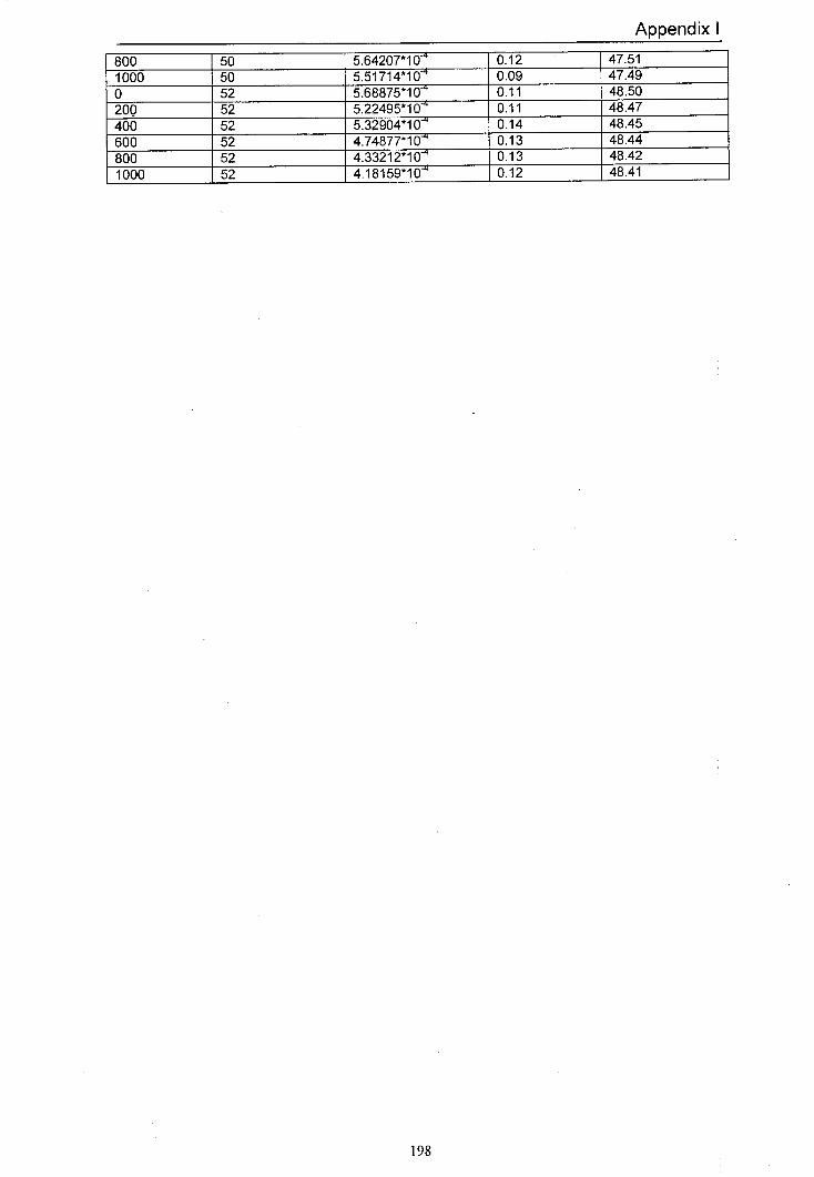
Appendix I
800 50 5.64207*10 4 0.12 47.51 1000 50 5.51714*10 0.09 47.49 0 52 5.68875*10 0.11 48.50
200 52 5.22495*10 0.11 48.47 400 52 5.32904*10* 0.14 48.45 600 52 4.74877*10* 0.13 1 48.44 800 52 4.33212*10 0.13 1 48.42
1000 52 4.18159*10 4 0.12 1 48.41
198
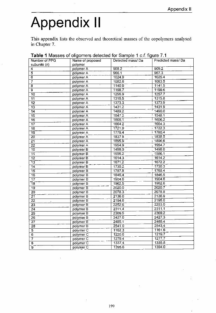
Appendix Ii
Appendix II This appendix lists the observed and theoretical masses of the copolymers analysed in Chapter 7.
Table I Masses of oligomers detected for Sample 1 c.f. figure 7.1 Number of PPG subunits (n)
Name of proposed polymer
Detected mass/ Da Predicted mass! Da
4 polymer A 908.2 909.2 5 polymer A 966.1 967.3 6 polymer 1024.9 1025.4 7 polymer 1082.6 1083.5 8 polymer 1140.9 1141.5 9 polymer 1198.7 1199.6 10 polymer 1256.9 1257.7 11 polymer 1315.5 1315.8 12 polymer 1373.3 1373.9 13 polymer 1431.2 1431.9 14 polymer A 1489.2 1490.0 15 polymer 1547.2 1548.1 16 polymerA 1605.1 1606.2 17 polymer 1664.2 1664.3 18 polymer 1721.9 1722.3 19 polymer 1779.4 1780.4 20 polymer 1837.8 1838.5 21 polymer A 1895.9 1896.6 22 polymer A 1954.9 1954.7 10 polymer B 1498.0 1498.0 11 - polymer B 1556.2 1556.1 12 polymer B 1614.3 1614.2 13 polymer B 1671.2 1672.2 14 polymer B 1730.2 1730.3 15 polymer B 1787.8 1788.4 16 polymer B 1846.4 1846.5 17 polymer B 1904.6 1904.6 18 polymer B 1962.5 1962.6 19 polymer B 2020.0 2020.7 20 polymer B 2078.3 2078.8 21 polymer B 2136.0 2136.9 22 polymer B 2194.6 2195.0 23 polymer B 2252.6 2253.0 24 polymer B 2311.4 2311.1 25 polymer B 2369.5 2369.2 26 polymer B 2427.0 2427.3 27 polymer B 2485.1 2485.4 28 polymer B 2541.0 2543.4 5 polymer 1162.3 1161.6 6 polymer C 1220.6 1219.7 7 polymer C 1279.4 _1277.7 8 polymer C 1337.4 1335.8 9 polymer C 1395.6 1 1394.0
199
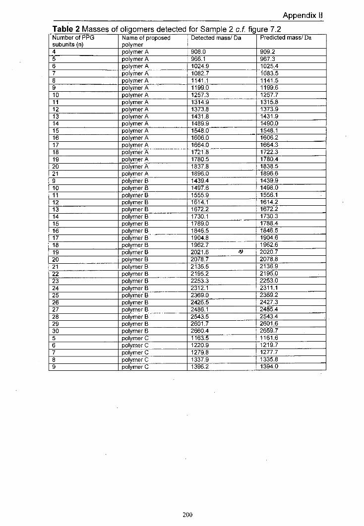
Appendix II
Table 2 Masses of oligomers detected for Sample 2 c.f. figure 7.2 Number of PPG subunits (n)
Name of proposed polymer
Detected mass! Da Predicted mass! Da
4 polymer A 908.0 909.2 5 polymer A 966.1 967.3 6 polymer A 1024.9 1025.4 7 polymer A 1082.7 1083.5 8 polymer 1141.1 1141.5 9 polymer 1199.0 1199.6 10 polymer 1257.3 1257.7 11 polymer 1314.9 1315.8 12 polymer 1373.8 1373.9 13 polymer 1431.8 1431.9 14 polymer 1489.9 1490.0 15 polymer 1548.0 1548.1 16 polymer A 1606.0 1606.2 17 polymer A 1664.0 1664.3 18 polymer 1721.8 1722.3 19 polymer 1780.5 1780.4 20 polymer A 1837.8 1838.5 21 polymer A 1896.0 1896.6 9 polymer B 1439.4 1439.9 10 polymer B 1497.6 1498.0 11 polymer B 1555.9 1556.1 12 polymer B 1614.1 1614.2 13 polymer B 1672.2 1672.2 14 polymer B 1730.1 1730.3 15 polymer B 1789.0 1788.4 16 polymer B 1846.5 1846.5 17 polymer B 1904.8 1904.6 18 polymer B 1962.7 1962.6 19 polymer B 2021.6 ' 2020.7 20 polymer B 2078.7 2078.8 21 polymer B 2136.5 2136.9 22 polymer B 2195.2 2195.0 23 polymer B 2253.3 2253.0 24 polymer B 2312.1 2311.1 25 polymer B 2369.0 2369.2 26 polymer B 2426.5 2427.3 27 polymer B 2486.1 2485.4 28 polymer B 2543.5 2543.4 29 polymer B 2601.7 2601.6 30 polymer B 2660.4 2659.7 5 polymer 1163.5 1161.6 6 polymer C 1220.9 1219.7 7 1 polymer C 1279.8 1277.7 8 1 polymer C 1337.9 1335.8 9 1 polymer C 1396.2 1394.0
200

Appendix II
Table 3 Masses of oligomers detected for Sample 3 cf. figure 7.4 Number of PPG subunits (n)
Name of proposed polymer
Detected mass/ Da Predicted mass! Da
3 polymer A 850.8 851.1 4 polymer A 909.2 909.2 5 polymer A 966.7 967.3 6 polymer A 1025.1 1025.4 7 polymer A 1083.3 1083.5 8 polymer 1141.1 1141.5 9 polymer 1199.3 1199.6 10 polymer 1257.9 1257.7 11 polymer 1315.8 1315.8 13 polymerA 1431.2 1431.9 14 polymer A 1490.6 1490.0 15 polymer 1547.8 1548.1 16 polymer A 1606.1 1606.2 17 polymer A 1664.3 1664.3 18 polymer 1722.3 1722.3 19 polymer 1781.3 1780.4 4 polymer 801.6 802.1 5 polymer D 859.2 860.1 6 polymer 917.9 918.2 7 polymer D 975.8 976.3 8 polymer D 1034.4 1034.4 9 polymer D 1092.8 1092.5 10 polymer 1150.8 1150.5 11 polymer 1208.3 1208.6 12 polymer D 1267.1 1266.7 13 polymer 1324.2 1324.8 14 polymer D 1382.5 1382.9 15 polymer D 1441.0 1440.9 16 polymer D 1499.5 1499.0 17 polymer D 1556.9 1557.1 18 polymer 1615.4 1615.2 19 polymer D 1673.7 1673.3 20 polymer 1730.7 1731.3 21 polymer D 1789.8 1789.4 5 polymer E 752.3 753.0 6 polymer 810.7 811.1 7 polymer E 868.6 869.2 8 polymer E 926.7 927.2 9 polymer E 984.8 985.3 10 polymer E 1042.8 1043.4 11 polymer 1100.5 1101.5 12 polymer 1158.7 1159.6 13 polymer E 1217.3 1217.6 14 polymer E 1275.4 1275.7 15 polymer 1332.6 1333.8 16 polymer 1392.2 1391.9 17 polymer E 1449.7 1450.0 18 polymer E 1507.3 1508.0 19 polymer E 1566.0 1566.1 20 polymer E 1623.5 1624.2 21 polymer 1681.9 1682.3 22 polymer 1739.1 1740.4 23 polymer 1797.1 1798.4
201
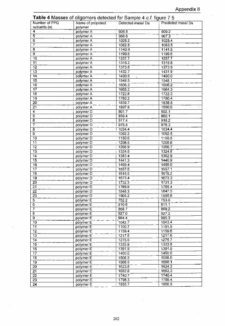
Appendix II
Table 4 Masses of oliqomers detected for Sample 4 c.f. figure 7.5 Number of PPG subunits (n)
Name of proposed polymer
Detected mass/ Da Predicted mass! Da
4 polymer A 908.8 909.2 5 polymer A 966.6 967.3 6 polymer 1025.2 1025.4 7 polymer 1082.8 1083.5 8 polymer 1140.9 1141.5 9 polymer 1199.6 1199.6 10 polymer A 1257.7 1257.7 11 polymer 1316.2 1315.8 12 polymer A 1373.8 1373.9 13 polymer 1432.7 1431.9 14 polymer A 1490.6 1490.0 15 polymer 1548.5 1548.1 16 polymer 1606.3 1606.2 17 polymer A 1665.2 1664.3 18 polymer 1722.8 1722.3 19 polymer A 1780.2 1780.4 20 polymer A 1839.7 1838.5 21 polymer A 1897.8 1896.6 4 polymer 801.7 802.1 5 polymer D 859.4 860.1 6 polymer 917.4 918.2 7 polymer D 975.5 976.3 8 polymer D 1034.4 1034.4 9 polymer D 1092.2 1092.5 10 polymer 1150.6 1150.5 11 polymer 1208.5 1208.6 12 polymer D 1266.9 1266.7 13 polymer 1324.5 1324.8 14 polymer D 1383.4 1382.9 15 polymer 1441.3 1440.9 16 polymer D 1499.4 1499.0 17 polymer D 1557.5, 1557.1 18 polymer 1615.5 1615.2 19 polymer D 1673.4 1673.3 20 polymer D 1732.3 1731.3 21 polymer D 1789.9 1789.4 22 polymer D 1848.3 1847.5 23 polymer 1905.2 1905.6 5 polymer E 752.2 753.0 6 polymer 810.6 811.1 7 polymer E 868.7 869.2 8 polymer E 927.0 927.2 9 polymer E 984.4 985.3 10 polymer 1042.7 1043.4 11 polymer 1100.7 1101.5 12 polymer 1159.4 1159.6 13 polymer E 1217.5 1217.6 14 polymer E 1275.0 1275.7 15 polymer . 1333.9 1333.8 16 polymer 1391.9 1391.9 17 polymer E 1450.0 1450.0 18 polymer E 1508.3 1508.0 19 polymer E 1566.5 1566.1 20 polymer 1623.5 1624.2 21 polymer E 1682.8 1682.3 22 polymer E 1740.7 1740.4 23 polymer 1798.3 1798.4 24 polymer 1855.7 1856.5
202

Appendix II
Table 5 Masses of oligomers detected for Sample 5 c.f. figure 7.6 Number of PPG subunits (n)
Name of proposed polymer
Detected mass/ Da Predicted mass! Da
5 polymer F 531.2 530.7 6 polymer F 589.2 588.8 7 polymer F 647.2 646.9 8 polymer F 705.5 704.9 9 polymer F 763.2 763.0 10 polymer F 821.5 821.1 11 polymer F 879.3 879.2 12 polymer F 937.3 937.3. 13 polymer F 996.3 995.3 14 polymer F 1054.3 1053.4 15 polymer F -- 1111.9 1111.5 16 polymer 1170.1 1169.6 17 polymer F 1227.8 1227.7 18 polymer F 1286.8 1285.7 19 polymer F 1345.1 1343.8 3 polymer G 669.3 668.9 4 polymer G 727.9 727.0 5 polymer G 785.6 785.0 6 polymer G 843.9 843.1 7 polymer 901.6 901.2 8 polymer G 960.4 959.3 9 polymer 1018.2 1017.4 10 polymer 1075.8 1075.4 11 polymer . 1135.0 1133.5 12 polymer 1192.8 1191.6 13 polymer 1252.0 1249.7 14 polymer 1309.6 1307.8 15 polymer G 1367.3 1365.8 16 polymer G 1425.2 1423.9 17 polymer G 1483.2 1482.0 18 polymer 1542.4 1540.1
203
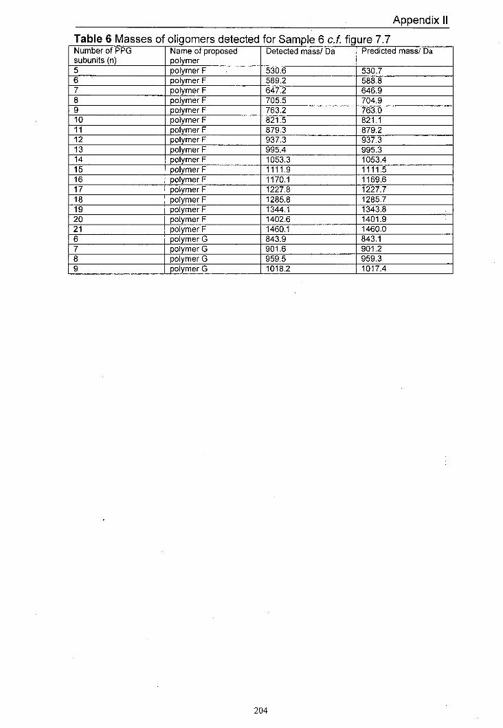
Appendix II
Table 6 Masses of oligomers detected for Sample 6 c.f. fiqure 7.7 Number of PPG subunits (n)
Name of proposed polymer
Detected mass/ Da Predicted mass! Da
5 polymer F 530.6 530.7 6 polymer F 589.2 588.8 7 polymer F 647.2 646.9 8 polymer F 705.5 704.9 9 polymer F 763.2 763.0 10 polymer F 821.5 821.1 11 polymer F 879.3 879.2 12 polymer F 937.3 937.3 13 polymer F 995.4 995.3 14 polymer F 1053.3 1053.4 15 polymer 1111.9 1111.5 16 polymer 1170.1 1169.6 17 polymer F 1227.8 1227.7 18 polymer F 1285.8 1285.7 19 polymer F 1344.1 1343.8 20 polymer F 1402.6 1401.9 21 polymer F 1460.1 1460.0 6 polymer G 843.9 843.1 7 polymer 901.6 901.2 8 polymer G 959.5 959.3 9 polymer 1018.2 1017.4
204