matrix and tensor-based esprit algorithm for joint angle
TRANSCRIPT

Matrix and Tensor-based ESPRIT Algorithm for Joint Angleand Delay Estimation in 2D Active Broadband Massive MIMO
SystemsAND
Analysis of Direction of Arrival Estimation Algorithms forBasal Ice Sheet Tomography
By
Yi Zhu
Submitted to the Electrical Engineering and Computer Science Department and theGraduate Faculty of the University of Kansas
in partial fulfillment of the requirements for the degree ofMaster of Science
Committee members
Dr. Lingjia Liu, Chairperson
Dr. John Paden
Dr. Erik Perrins
Dr. Shannon Blunt
Date defended: August 6, 2014

The Dissertation Committee for Yi Zhu certifiesthat this is the approved version of the following dissertation :
Matrix and Tensor-based ESPRIT Algorithm for Joint Angle and Delay Estimation in 2D ActiveBroadband Massive MIMO Systems
ANDAnalysis of Direction of Arrival Estimation Algorithms for Basal Ice Sheet Tomography
Dr. Lingjia Liu, Chairperson
Dr. John Paden
Dr. Erik Perrins
Dr. Shannon Blunt
Date approved: August 6, 2014
i

Abstract
In this thesis, we apply and analyze three direction of arrival algorithms (DoA) to
tackle two distinct problems: one belongs to wireless communication, the other to
radar signal processing. Though the essence of these two problems is DoA estimation,
their formulation, underlying assumptions, application scenario, etc. are totally differ-
ent. Hence, we write them separately, with ESPRIT algorithm the focus of Part I and
MUSIC and MLE detailed in Part II.
For wireless communication scenario, mobile data traffic is expected to have an ex-
ponential growth in the future. In order to meet the challenge as well as the form
factor limitation on the base station, 2D massive MIMO has been proposed as one of
the enabling technologies to significantly increase the spectral efficiency of a wireless
system. In massive MIMO systems, a base station will rely on the uplink sounding
signals from mobile stations to figure out the spatial information to perform MIMO
beamforming. Accordingly, multi-dimensional parameter estimation of a ray-based
multipath wireless channel becomes crucial for such systems to realize the predicted
capacity gains. In the first Part, we study joint angle and delay estimation for 2D
massive MIMO systems in mobile wireless communications. To be specific, we first
introduce a low complexity time delay and 2D DoA estimation algorithm based on
unitary transformation. Some closed-form results and capacity analysis are involved.
Furthermore, the matrix and tensor-based 3D ESPRIT-like algorithms are applied to
jointly estimate angles and delay. Significant improvements of the performance can
be observed in our communication scheme. Finally, we found that azimuth estimation
is more vulnerable compared to elevation estimation. Results suggest that the dimen-
ii

sion of the antenna array at the base station plays an important role in determining the
estimation performance. These insights will be useful for designing practical massive
MIMO systems in future mobile wireless communications.
For the problem of radar remote sensing of ice sheet topography, one of the key re-
quirements for deriving more realistic ice sheet models is to obtain a good set of basal
measurements that enables accurate estimation of bed roughness and conditions. For
this purpose, 3D tomography of the ice bed has been successfully implemented with
the help of DoA algorithms such as MUSIC and MLE techniques. These methods
have enabled fine resolution in the cross-track dimension using synthetic aperture radar
(SAR) images obtained from single pass multichannel data. In Part II, we analyze and
compare the results obtained from the spectral MUSIC algorithm and an alternating
projection (AP) based MLE technique. While the MUSIC algorithm is more attrac-
tive computationally compared to MLE, the performance of the latter is known to be
superior in most situations. The SAR focused datasets provide a good case study to
explore the performance of these two techniques to the application of ice sheet bed
elevation estimation. For the antenna array geometry and sample support used in our
tomographic application, MUSIC performs better originally using a cross-over anal-
ysis where the estimated topography from crossing flightlines are compared for con-
sistency. However, after several improvements applied to MLE, i.e., replacing ideal
steering vector generation with measured steering vectors, automatic determination of
the number of scatter sources, smoothing the 3D tomography in order to get a more
accurate height estimation and introducing a quality metric for the estimated signals,
etc., MLE outperforms MUSIC. It confirms that MLE is indeed the optimal estimator
for our particular ice bed tomographic application. We observe that, the spatial bot-
tom smoothing, aiming to remove the artifacts made by MLE algorithm, is the most
essential step in the post-processing procedure. The 3D tomography we obtained lays
a good foundation for further analysis and modeling of ice sheets.
iii

Acknowledgements
I wish to extend my deepest gratitude to my advisor Dr. Lingjia Liu for his encour-
agement, guidance and patience during the course of this thesis. The experience I
have gained during my association with both ITTC and CReSIS has been invaluable.
I would also like to thank Dr. John Paden, Dr. Shannon Blunt and Dr. Erik Perrins
for their time and kindness to serve on the committee, and helpful advise towards the
fulfilment of the dissertation. Especially to Dr. John Paden, I am extremely grateful
for the work opportunity he provided, the practical programming skills he taught and
enormous help during my writing of second part of the thesis. My sincere gratitude to
Dr. Victor Frost and Pam Shadoin for being patient and affording me an opportunity to
complete this work. I also want to thank Dr. David Petr and Dr. Sam Shanmugan for
their wonderful courses, which benefits me a lot for my future study. Finally, I would
like to thank my parents, my girlfriend and all my friends in University of Kansas for
their constant encouragement and immense support.
iv

Contents
I Matrix and Tensor-based ESPRIT Algorithm for Joint Angle and De-
lay Estimation in 2D Active Broadband Massive MIMO Systems 1
1 Introduction 2
2 System Model 5
2.1 Channel Model Estimation . . . . . . . . . . . . . . . . . . . . . . . . . . . . . . 5
2.2 ESPRIT-based Delay Estimation . . . . . . . . . . . . . . . . . . . . . . . . . . . 10
3 2D Joint DoA Estimation 13
3.1 2D DoA Estimation Data Model . . . . . . . . . . . . . . . . . . . . . . . . . . . 13
3.2 Low Complexity 2D DoA Estimation . . . . . . . . . . . . . . . . . . . . . . . . 15
4 Joint Angle and Delay Estimation 21
4.1 Matrix-based Joint Estimation Using Standard ESPRIT . . . . . . . . . . . . . . . 21
4.2 Real processing and Automatic-pairing . . . . . . . . . . . . . . . . . . . . . . . . 23
4.2.1 3D extension of Unitary ESPRIT . . . . . . . . . . . . . . . . . . . . . . 24
4.2.2 Forward-Backward Averaging . . . . . . . . . . . . . . . . . . . . . . . . 26
4.2.3 Joint diagonalization . . . . . . . . . . . . . . . . . . . . . . . . . . . . . 28
5 Tensor-based JADE Using ESPRIT 31
5.1 Basic tensor notation and operation . . . . . . . . . . . . . . . . . . . . . . . . . . 31
5.2 Tensor-based Joint Estimation Using Standard ESPRIT . . . . . . . . . . . . . . . 33
v

5.3 Matrix and Tensor-based Unitary ESPRIT Algorithm Simulation . . . . . . . . . . 38
5.3.1 Comparison between 2D Joint Angle Estimation and Matrix-based 3D
JADE Estimation . . . . . . . . . . . . . . . . . . . . . . . . . . . . . . . 39
5.3.2 Comparison between 3D Matrix and Tensor-based JADE Algorithm . . . . 41
6 Conclusion and Future Work 44
II Analysis of Direction of Arrival Estimation Algorithms for Basal Ice
Sheet Tomography 47
7 Introduction 48
8 Modeling and Approaches 51
8.1 Overview . . . . . . . . . . . . . . . . . . . . . . . . . . . . . . . . . . . . . . . 51
8.2 System model . . . . . . . . . . . . . . . . . . . . . . . . . . . . . . . . . . . . . 52
8.3 MUSIC . . . . . . . . . . . . . . . . . . . . . . . . . . . . . . . . . . . . . . . . 55
8.4 Maximum Likelihood Localization by Alternating Projection . . . . . . . . . . . . 56
8.4.1 Maximum Likelihood Estimator . . . . . . . . . . . . . . . . . . . . . . . 57
8.4.2 The Alternating Projection Technique . . . . . . . . . . . . . . . . . . . . 60
8.4.2.1 Alternating Maximization Technique . . . . . . . . . . . . . . . 60
8.4.2.2 Projection Matrix Decomposition . . . . . . . . . . . . . . . . . 61
9 Dataset Analysis 64
9.1 Application of Algorithms . . . . . . . . . . . . . . . . . . . . . . . . . . . . . . 64
9.1.1 MUSIC . . . . . . . . . . . . . . . . . . . . . . . . . . . . . . . . . . . . 65
9.1.2 MLE-AP . . . . . . . . . . . . . . . . . . . . . . . . . . . . . . . . . . . 65
9.1.2.1 Measured Steering Vectors . . . . . . . . . . . . . . . . . . . . 66
9.1.2.2 Model Order Statistics . . . . . . . . . . . . . . . . . . . . . . . 69
9.1.2.3 Bottom Smoothing . . . . . . . . . . . . . . . . . . . . . . . . . 71
vi

9.1.2.4 Speed Up MLE-AP . . . . . . . . . . . . . . . . . . . . . . . . 76
9.2 Output From Greenland Dataset . . . . . . . . . . . . . . . . . . . . . . . . . . . 77
10 Conclusion and Future Work 86
vii

List of Figures
2.1 Model of 2D “Massive MIMO” System . . . . . . . . . . . . . . . . . . . . . . . 5
3.1 Unitary Joint Elevation Angle Estimation . . . . . . . . . . . . . . . . . . . . . . 19
3.2 Unitary Joint Azimuth Angle Estimation . . . . . . . . . . . . . . . . . . . . . . . 19
3.3 Unitary Separate Delay Estimation . . . . . . . . . . . . . . . . . . . . . . . . . . 20
5.1 Comparison Between 2D Separate and 3D Matrix-based Joint Delay Estimation . . 39
5.2 Comparison Between 2D Joint and 3D Matrix-based Joint Elevation Angle Esti-
mation . . . . . . . . . . . . . . . . . . . . . . . . . . . . . . . . . . . . . . . . . 40
5.3 Comparison Between 2D Joint and 3D Matrix-based Joint Azimuth Angle Estimation 41
5.4 Comparison Between 3D Matrix and Tensor-based Joint Delay Estimation . . . . . 41
5.5 Comparison Between 3D Matrix and Tensor-based Joint Elevation Angle Estimation 42
5.6 Comparison Between 3D Matrix and Tensor-based Joint Azimuth Angle Estimation 43
7.1 Synthetic Aperture Radar System Geometry for Left and Right Swaths . . . . . . 49
8.1 Coordinate System for Radar 3D Imaging . . . . . . . . . . . . . . . . . . . . . . 53
8.2 Terrain returns and image signatures for a pulse of radar energy . . . . . . . . . . . 54
9.1 Angle Distribution of Steering Vectors for Multi-channels . . . . . . . . . . . . . . 68
9.2 Angle Distribution and Difference of Steering Vectors for Multi-channels . . . . . 69
9.3 Magnitude Distribution of Corrected Measured Steering Vectors Generation . . . . 69
9.4 DoA Distribution Using MLE Focusing on Bottom Region. . . . . . . . . . . . . 73
viii
9.5 DoA Estimation Using MLE for First Record of Frame 20130410 01 033 . . . . . 75
9.6 DoA Distribution Using MUSIC Focusing on Bottom Region. . . . . . . . . . . . 76
9.7 Flight Pattern and Echograms . . . . . . . . . . . . . . . . . . . . . . . . . . . . . 78
9.8 DEM From a Single Pass Using the MLE Algorithm . . . . . . . . . . . . . . . . 79
9.9 Cross-Over Analysis by MUSIC . . . . . . . . . . . . . . . . . . . . . . . . . . . 80
9.10 Cross-Over Analysis by MLE Without Bottom Smoothing . . . . . . . . . . . . . 81
9.11 Cross-Over Analysis by MLE With Bottom Smoothing . . . . . . . . . . . . . . . 81
9.12 Cross-Over Analysis by MLE With Measured Steering Vectors . . . . . . . . . . . 82
9.13 Cross-Over Analysis by MLE With Model Order Statistics . . . . . . . . . . . . . 82
9.14 Cross-Over Analysis by MLE With Quality Metric . . . . . . . . . . . . . . . . . 84
ix

List of Tables
9.1 Difference Statistics Comparison between MUSIC and Various Applications of
MLE-AP Algorithm . . . . . . . . . . . . . . . . . . . . . . . . . . . . . . . . . 83
x

Part I
Matrix and Tensor-based ESPRIT
Algorithm for Joint Angle and Delay
Estimation in 2D Active Broadband Massive
MIMO Systems
1

Chapter 1
Introduction
Rarely have technical innovations changed everyday life as rapidly and profoundly as mobile
wireless communications. According to the International Telecommunication Union (ITU) [1],
the number of mobile wireless subscriptions globally reached 6.8 billions in 2013, almost as many
as the world population 7.1 billions. As a result, in February 2013, Cisco Systems predicted a
staggering 66% compound annual growth rate (CAGR) for global mobile data traffic from 2012 to
2017 [2]. This is an 13-fold increase in wireless traffic over a five-year period.
A key societal question and a pressing engineering challenge is: “How can we support the pre-
dicted exponential growth in mobile data traffic?” To meet the increasing traffic demand, other than
reallocating radio spectrum to wireless providers, spectral efficiency will need to be improved sig-
nificantly. Multiple-input-multiple-out (MIMO) technology, together with Orthogonal frequency-
division multiplexing (OFDM), offer efficient ways to increase the spectral efficiency of a mobile
broadband communication system [3]. Recently, a new MIMO paradigm called “massive MIMO”
has generated much interests in both academia [4, 5] and industry [6]. Using information theoreti-
cal analysis, it can be shown that even with random user scheduling and no inter-cell cooperation,
unprecedented spectral efficiency in time-division-duplex (TDD) cellular systems can be achieved
if a sufficiently large number of transmit antennas are employed at each base station.
Because of the sensitivity of MIMO algorithms with respect to the channel matrix properties,
2

channel modeling is particularly critical to assess the performance of underlying MIMO systems.
The parametric channel model could be adopted by performing virtual direction-of-arrival (DoA)
and direction-of-departure (DoD) estimation of resolvable paths. It provides a simple geometric
interpretation of the scattering environment to characterize the two key MIMO channel metrics:
ergodic capacity and diversity level [7]. Despite the advantage of reducing the number of estima-
tion parameters, it is shown in [8] that channel estimation based on DoA and DoD provides the
best performance in terms of the error bound.
Due to the form factor limitation, two-dimensional (2D) MIMO systems are introduced re-
garding elevation and azimuth domain, to fit a large number of antenna elements on the base
station in reality. For a base station equipped with such planar arrays, it needs to know the corre-
sponding multi-dimensional channel knowledge. There are many existing subspace-based methods
such as MUSIC (MUltiple SIgnal Classification), ESPRIT and matrix pencil to estimate the one-
dimensional (1D) DoA under parametric channel models. However, its counterpart in 2D, together
with delay estimation is not yet well explored. The TST-MUSIC algorithm proposed in [9] have
great performance in estimating the DoAs and delay of a wireless multi-ray channel, but the pairing
of the 2-D angles and delay can’t be automatically determined, which means two signals with close
parameters are indistinguishable. In [10], the authors just show the M-dimensional estimation of
spatial frequencies using tensor modeling without mentioning the individual physical parameters
estimation, which are crucial for practical MIMO transceiver design.
The main reason why we choose ESPRIT algorithm over MUSIC is the existence of MIMO
antenna array at the base station. ESPRIT has made signal-subspace based methods more attractive
for implementation because the array manifold matrix need not be known and the search procedure
is replaced by a simple eigenvalue problem. Especially when there are plenty of sensors compared
with the number of sources to detect, ESPRIT is much more suitable than MUSIC and MLE with
respect to the computational burden. Though for minimum squared error (MSE) perspective, MLE
and MUSIC outperforms ESPRIT in most circumstances. Generally, we are satisfied with the
results obtained from ESPRIT since it is also a super-resolution estimation technique.
3

Hence, in our paper, we define a natural tensor-based system model for the application of joint
angle and delay estimation (JADE) and intense computer simulations are conducted. By jointly es-
timating the channel parameters, DoA estimation could give us accurate spatial information about
the four-dimensional (4D) underlying physical channel which is crucial for transmit precoding.
Simulation results indicate the superiority of tensor in terms of estimation performance due to an
improved signal subspace estimate.
The rest of the thesis is organized as follows. In Chapter 2, the 3D system model used in this
paper is described. Simplest separate estimation of channel parameters is introduced as preliminary
work. In Chapter 3, we jointly estimate the elevation and azimuth angle using standard ESPRIT
algorithm and then extend it into real processing domain by unitary transformation. Simulation re-
sults suggests that azimuth angle estimation performance is more vulnerable compared to elevation
angle estimation. Impact of various antenna configurations onto estimation of MSE is investigated.
In Chapter 4, we present the matrix-based 3D joint angle and delay estimation approach and its
extension to 3D unitary ESPRIT algorithm. Furthermore, automatic pairing is achieved through a
modified simultaneous Schur decomposition (SSD) [11]. We derive a tensor-based 3D JADE sys-
tem model and naturally extends all the previous results for matrix case in Chapter 5. A detailed
performance comparison between separate and joint estimation / matrix and tensor-based approach
is given under various antenna configurations. It shows us how dimensionality and practical im-
plementation will impact the channel estimation performance of a 2D antenna array at the base
station. Finally, Chapter 6 concludes the thesis and we show a list of active research topics needed
to be studied in the future.
4

Chapter 2
System Model
2.1 Channel Model Estimation
A typical 2D “Massive MIMO” system with an M1×M2 antenna array at the base station can
be shown in Fig. 2.1 [12]. In this particular system, a base station is at the height of h while a
Y
X
Z
d
d
h
hm
Ɵ
ɸ
Figure 2.1: Model of 2D “Massive MIMO” System
mobile station is at the height of hm. The antenna array at the base station is a planar array placed
5

in the X-Z domain with M1 antenna elements vertically and M2 antenna elements horizontally.
The spacing between adjacent sensors is assumed to be d, without loss of generality, we fix it to
the critical half wavelength distance in order to avoid the spatial spectrum alias. Since the matrix
factorization form of the channel will get rather complicated for the case where both transmitter
and receiver are equipped with multiple antennas. For simplicity, throughout this paper we assume
that there is only one transmit antenna at the mobile station, which is also the typical scenario for
modern cellular systems. Under this assumption, the transmit antenna array steering becomes a
scalar which we normalize to 1. In the 2D “Massive MIMO” system, instead of mechanical down-
tilting the antenna array towards the mobile station, the base station could also perform digital
beamforming in both elevation and azimuth domain, because 2D DoA estimation will provide the
base station some channel knowledge on the downlink.
In reality, the propagation situation in a wireless communication system is rather complicated.
The uplink sounding reference signals usually go through scattering, reflection, refraction, and
diffraction before they reach the base station. For a multi-path scenario, a wireless channel is
usually modeled by a finite number of rays, each parameterized by a complex amplitude, spatial
angle and time delay, a.k.a the multi-ray propagation model.
In this paper, we derive a data model for the reception of a single source in a multi-path sce-
nario. Assume we transmit a digital sequence sk over a channel, and measure the response using
M1×M2 antennas. The noiseless received data Y (t) in general has the form
Y (t) = ∑k
sk H(t− kT ). (2.1)
where T is the symbol rate and for notation simplicity, it will be normalized to T = 1 from now
on. We writes the M1×M2 impulse response as
H(t) =P
∑ℓ=1
αℓ a(uℓ)aT (vℓ)g(t− τℓ). (2.2)
where g(t) is a known pulse shape function by which sk is modulated. In our scenario, there
6

are P distinct propagation paths and we assume the number P is available. Many of the signal
detection methods are applicable to our model, e.g., the methods based on the AIC and MDL
principle, since the path fading are normally distributed. Detailed performance comparison of
these two criteria on model order statistics will be shown in Part II. αℓ denotes the complex en-
velope of the ℓth fading path. The vector-valued function a(uℓ) = [1,e juℓ, · · · ,e j(M1−1)uℓ]T and
a(vℓ) = [1,e jvℓ, · · · ,e j(M2−1)vℓ]T can be viewed as the steering vectors of elevation angle and az-
imuth angle respectively. uℓ = 2πdλ cosθℓ,vℓ = 2πd
λ sinθℓ cosϕℓ represent two spatial frequencies of
path ℓ according to our base station array configuration, λ is the wavelength.
Note that, our application is for wireless communication and the data model above indicates
a broadband communication system. However, for further array signal processing, we need to
make a narrowband phased array assumption. The narrowband signal and narrowband array are
two different concepts, because the actual signal bandwidth alone cannot be used to categorize a
signal as being narrowband or broadband. For different sensor arrays or even for different emitter
locations relative to the array, the same signal may fall into either category. If B is the band width
of the signal and Tmax is the maximum time required by the signal to cross the array, then the
situation below is considered as a narrowband array case
B×Tmax ≤ 1. (2.3)
Obviously, this equation also depends upon the DoA and array geometry, therefore the same signal
can be considered broadband or narrowband depending upon these parameters. Now, if we focus
on azimuth domain, which is the general 1D uniform linear array case, we can find that as the
direction of arrival angle approaches to 90, Tmax approaches to 0 and when angle approaches to 0,
Tmax becomes larger. Moreover, Tmax is also proportional to number of sensors in the array.
Since for broadband array scenario, the array steering vector will be frequency-dependent. In
other words, if we assume a broadband antenna array, the delay between antenna elements can-
not be approximately translated into phase shift in frequency domain, and no more Vandermonde
7

structure can be exploited. In this situation, the array manifold matrix varies significantly over
the range of frequencies present and the ordinary signal-subspace approach fails. In particular,
the spatial covariance matrix of the sensor output matrix generally has full rank, even for a single
broadband signal. And this matrix cannot be used to define the signal subspace for the broadband
case. Hence, we tackle this mobile communication problem under the narrowband array condition
for the rest of the thesis.
Now, we need to stack dimensions through collecting all the array responses from an M1×M2
steering matrix A(uℓ,vℓ) = a(uℓ)aT (vℓ). To be specific, let aℓ be the vector after the mapping of
matrix A(uℓ,vℓ), it can be shown that:
aℓ = a(vℓ)⊗a(uℓ)
where ⊗ is the Kronecker product. From aℓ, we can construct a 2D steering matrix of the received
signals, A = [a1,a2, . . . ,aP] ∈ CM1M2×P, which contains all the information related to the P path
signals whose elevation angle θℓ and azimuth angle ϕℓ are to be estimated.
It is reasonable to assume that the known modulation pulse shape function g(t) has finite
support [0,Lg). With τmax = max1≤ℓ≤P
τℓ denotes the maximum delay spread, the channel length is
L = Lg + τmax, which means the channel impulse response h(t) has finite duration and is zero
outside an interval [0,L) [13]:
h(t) =P
∑ℓ=1
αℓ aℓ g(t− τℓ) (2.4)
where L and Lg are both measured in symbol periods. Thus the received data Y (t) can be re-
organized into an M1M2×1 vector y(t) for the time series data model. We assume that the received
data is sampled at a rate of V times the symbol rate. Using either training sequences (known sk)
or blind channel estimation techniques, it is possible to estimate h(k), k = 0, 1P , · · · ,L−
1V , at least
up to a scalar. Specifically, suppose we start sampling at t = 0 and collect samples of y(t) during
8

N symbol periods, the noiseless received data can be rewritten in compact form as
Yv = Hv S (2.5)
Herein,
Yv =
y(0) y(1) · · · y(N−1)
y( 1V ) y(1+ 1
V ) · · · y(N−1+ 1V )
...... . . . ...
y(1− 1V ) y(2− 1
V ) · · · y(N− 1V )
Hv =
h(0) h(1) · · · h(L−1)
h( 1V ) h(1+ 1
V ) · · · h(L−1+ 1V )
...... . . . ...
h(1− 1V ) h(2− 1
V ) · · · h(L− 1V )
.
S =
s0 s1. . . sN−1
s−1 s0 s1. . .
. . . . . . . . . . . .
s−(L−1) s−(L−2) · · · s−(L−N)
where Yv represents the M1M2V ×N vectorized received data matrix while S is the L×N sym-
bol matrix with Toeplitz structure. Note that, if transmitted sequence s(k) is known for k =
−L+ 1, · · · ,N− 1 and N ≥ L, we can directly estimate the M1M2V × L channel matrix through
least-square type of methods and apply JADE algorithm, i.e., Hv = YvS†, where the superscript †
represents matrix pseudo-inverse.
It is convenient to rearrange the estimated impulse response samples into an M1M2×LV chan-
nel matrix H1 similarly as (2.4), including all the components: the array response, fading parame-
9

ters, symbol waveform and path delay:
H1 =
a1 · · · aP
α1
. . .
αP
g(τ1)
...
g(τP)
= ABG
(2.6)
where B is the P×P diagonal matrix containing complex fading envelope. G denotes the P×LV
time delay matrix, where g(τℓ) = [g(k− τℓ)]k=0,1/V,··· ,L−1/V is a 1×LV row vector of samples of
g(t− τℓ). At this point, we can easily solve the joint azimuth-elevation estimation problem using
2D ESPRIT techniques [12], as long as we have the channel estimate. We will discuss it in more
detail within chapter 3.
2.2 ESPRIT-based Delay Estimation
In this section, we will introduce the delay estimation algorithm using shift-invariance struc-
ture, by the fact that a Fourier transform maps a delay to phase progression. Usually, the pulse
shaping function g(t) is assumed to be raised cosine roll-off signal because of its capability in
reducing inter symbol interference (ISI) from multi-path signal reflections. As in our model, the
known transmitted waveform g(t) is sampled at a rate of V times and we denote the 1×LV row
vector as:
g = [g(0),g( 1V ), · · ·g(L−
1V )] (2.7)
10

Here, we use a discrete Fourier transform (DFT) to the samples of time sequence as GF = g FDFT ,
where FDFT represents the DFT matrix of size LV ×LV .
GF = g FDFT = g
1 1 · · · 1
1 Φ · · · Φ(LV−1)
...... . . . ...
1 Φ(LV−1) · · · Φ(LV−1)2
, Φ = e− j 2π
LV
Obviously, if τℓ is an integer multiple of 1V , we can directly obtain:
GF(τℓ) = [1,ΦτℓV ,Φ2τℓV , · · · ,Φ(LV−1)τℓV ] diag[GF ]
Note that, this equation holds true for any τ if g(t) is bandlimited and sampled at or above the
Nyquist rate, and these two inherent assumptions are reasonable to make in most circumstances
within digital communication area. The channel matrix in (2.6) after DFT transformation
HF = H1 FDFT
can be shown as:
HF = AB
1 ψ1 · · · ψLV−11
1 ψ2 · · · ψLV−12
......
......
1 ψP · · · ψLV−1P
diag(GF)
= ABFdiag(GF)
where ψℓ = e− j 2πL τℓ, ℓ= 1,2, · · · ,P. From the above equation, it is clear that the phase shift matrix
F is a Vandermonde matrix, which reminds us of the ESPRIT algorithm. If the matrix diag(GF) is
11
nonsingular, we can have:
HF = HF · diag(GF)−1 = ABF (2.8)
In order to apply the standard ESPRIT algorithm, we should transpose the above channel model
HF to reverse the matrices multiplication order. Let Fψ denote the transposed time delay matrix,
we can obtain:
Hτ = (HF)T = Fψ(AB)T . (2.9)
Note that, the role of Fψ equals to the array steering matrix in our former data model [12], which
means the delay estimation problem has been transformed to a typical DoA estimation problem.
If the number of multi-paths is not larger than the number of antennas (e.g., P≤M1 and P≤M2),
then we can follow our line of work to obtain ψℓ, as well as the parameter of interest τℓ through
shift-invariance property of the transposed channel matrix Hτ , independent of the structure of A.
However, in general, the number of antennas is limited and might not satisfy the condition (P > M1
and P > M2). This problem can be avoided by constructing a Hankel matrix out of HF , and we will
explain more in section 4.1 of chapter 4. By this mean, we can have various antenna configurations
even for two antenna elements on one direction.
From equation (2.8) and (2.9) it is clear that the angles and delay can be estimated indepen-
dently of each other, by directly working on the rows and columns of the transformed channel
matrix Hτ . However, this does not give a pairing between angles and the corresponding delay, and
might result in poor resolution for closely spaced angles and delays. We will introduce the 3D joint
angle and delay estimation algorithm for rectangular planar array in chapter 4.
12

Chapter 3
2D Joint DoA Estimation
3.1 2D DoA Estimation Data Model
For simplicity and comparison purpose, we first settle 2D joint angle estimation problem before
we approach the 3D joint one. All system settings remain the same except for the absence of delay,
thus we simply rewrite the channel matrix as:
Ha =P
∑ℓ=1
αℓ a(uℓ)aT (vℓ) (3.1)
Alternatively, we can use center of the antenna array as reference point because conjugate symme-
try property can significantly reduce the computational complexity, but it won’t make any differ-
ence to our subsequent algorithm procedure.
From (3.1), it can be seen that for the case where there is only one transmit antenna at the
mobile station the uplink channel completely depends on the DoA at the base station array. In
time-division-duplex (TDD) systems, there exists a reciprocity property between uplink channel
and the downlink channel. Therefore, the base station could potentially conduct downlink MIMO
operations for 2D “massive MIMO” systems based on the DoA estimation from the uplink. This
is also the reason why DoA estimation is critical for 2D “massive MIMO” systems.
Similarly, after vectorization, the channel matrix now is a M1M2×P matrix, denoted by Hav.
13

Accordingly, the M1M2×K received data matrix Yav (after the vector mapping) for K snapshots
can be written as
Yav = HavSa +Nav,
where Sa = [s1,s2, . . . ,sP]T are the P×K transmitted signals at the mobile device, and sℓ = [sℓ1,sℓ2,
. . . ,sℓK]. Here the signals s1,s2, . . . ,sP should be the same for our single source multi-path scenario.
Nav denotes the vectorized M1M2×K AWGN noise matrix, with noise power σ2n at each receiver
antenna element. Note that after rearranging the received signals into the steering matrix form, the
system model of the 2D antenna array is exactly the same as that of the 1D antenna array.
Using the standard estimation of signal parameters via rotational invariance techniques (ES-
PRIT) algorithm [14], a common model with shift invariance property can be given by
A0Φ = A1,
where A0 stands for the first M2−1 rows and A1 stands for the last M2−1 rows of the M1 blocks
of the transposed steering matrix A (aiming to estimate spatial frequency vℓ first). Φ is a diagonal
matrix whose entries are the phase shift of adjacent elements horizontally. Let Us be the MN×P
matrix of signal eigenvectors. Since the steering vectors in matrix A span the same subspace as Us,
there exists an invertible matrix T such that Us = AT . Constructing matrices Us0 and Us1 from Us
as A0 and A1 from A, and let the transition matrix Ψ = T−1ΦT , we have
Us1 =Us0Ψ. (3.2)
Note that the matrix Φ is a diagonal matrix containing the eigenvalues of Ψ. Using total least
square method, we will be able to solve equation (3.2) to obtain the estimated spatial frequencies
of vℓ and similar to the spatial frequencies of uℓ. In 2D “massive MIMO” systems, the two spatial
frequencies uℓ and vℓ in the steering matrix are related to the elevation and azimuth angles of
incoming signals we are interested in. There are many existing methods, especially subspace-
14

fitting based, to estimate the 2D DoA corresponding to this typical system model, e.g., MUSIC,
matrix pencil and ESPRIT. However, the computational complexity of these original algorithms is
prohibitively high.
3.2 Low Complexity 2D DoA Estimation
In this section, we will introduce a low complexity approach based on unitary ESPRIT algo-
rithm to jointly estimate the elevation and azimuth angles. The unitary transformation (a.k.a. real
processing) will convert complex matrices to real matrices, and all subsequent operations to the
real domain, with obvious computational and numerical advantages.
As discussed in section 2.1, the array manifold matrix of an M1×M2 antenna array can be
expressed as A(uℓ,vℓ) = a(uℓ)aT (vℓ), that is, the 2D steering matrix can be decomposed to the
product of two 1D steering vectors.
For a(ui), if the first (M1−1) elements are multiplied by e juℓ , the resulting vector will be equal
to the last (M1−1) components. This can be expressed as:
e juℓJ1a(uℓ) = J2a(uℓ) (3.3)
where J1 is an (M1−1)×M1 matrix constructed by taking the first (M1−1) rows of IM1 (M1×M1
identity matrix) and J2 is the (M1−1)×M1 matrix constructed by taking the last(M1−1) rows of
IM1 . A unitary matrix, QM1 , can be constructed to change the steering vector to real values. That
is,
aR(uℓ) = QHM1
a(uℓ),
Assuming M1 = 2q which is an even number, QM1 can be constructed as
Q2K =1√2
Iq jIq
Πq jΠq
,
15

where Iq is the q× q unit matrix, and ΠM is the M×M exchange matrix with ones on the anti-
diagonal and zeros elsewhere. Since QM1 is unitary, we can rewrite (3.3) as
e juℓJ1QM1QHM1
a(uℓ) = J2QM1QHM1
a(uℓ). (3.4)
Multiplying QHM1−1 on both sides gives us
e juℓQHM1−1J1QM1aR(uℓ) = QH
M1−1J2QM1aR(uℓ). (3.5)
It can be shown that QHM1−1J2QM1 =
(QH
M1−1J1QM1
)∗. Let K1 = Re
QH
M1−1J2QM1
, and K2 =
Im
QHM1−1J2QM1
. We can have the following relation:
tan(uℓ
2
)K1aR(uℓ) = K2aR(uℓ) (3.6)
We can extend the relation to 2D antenna array
tan(uℓ
2
)K1AR(uℓ,vℓ) = K2AR(uℓ,vℓ), (3.7)
where
AR(uℓ,vℓ) = QHM1
a(uℓ)aT (vℓ)Q∗M2= aR(uℓ)(aR(vℓ))T .
Let vec· be the vector operation, we can rewrite the formulation in (3.7) as
tan(uℓ
2
)Kx1vec
AR(uℓ,vℓ)
= Kx2vec
AR(uℓ,vℓ)
where Kx1 , IM2 ⊗K1, and Kx2 , IM2 ⊗K2. Accordingly, we can specify an M1M2×P real array
manifold matrix:
AR ,[vec
aR(u1,v1), . . . ,vec
aR(uP,vP)
]
16

Accordingly, we have
Kx1ARΩx = Kx2AR (3.8)
where
Ωx , diag
tan(u1
2
), tan
(u2
2
), . . . , tan
(uP
2
)It is important to note that after the unitary transformation, the matrices become real matrices.
Hence, all the subsequent operations turn to be real processing. This will significantly reduce the
computational complexity.
Similarly, for a(vℓ), we can conduct the same process. Let K3 = Re
QHM2−1J′2QM2
, and
K4 = Im
QHM2−1J′2QM2
, where J′2 is the (M2− 1)×M2 matrix constructed by taking the last
(M2−1) rows of IM2 . Accordingly, we have
Ky1ARΩy = Ky2AR (3.9)
where Ky1 , K3⊗ IM1 , Ky2 , K4⊗ IM1 , and
Ωy , diag
tan(v1
2
), tan
(v2
2
), . . . , tan
(vP
2
)(3.10)
Let Us be the signal subspace and T be the linear transformation matrix. Since the signal
subspace and the steering vector spans the same subspace, we have Us = ART . Substituting this
relation into (3.8), we have
Kx1Usϒx = Kx2Us (3.11)
where ϒx , T−1ΩxT . Similarly, we can also have
Ky1Usϒy = Ky2Us (3.12)
where ϒy , T−1ΩyT .
From (3.11) and (3.12), we can solve for ϒx and ϒy based on the estimated signal subspace Us.
17

Let the eigenvalues of the P×P complex matrix ϒx + jϒy be λℓ, ℓ = 1,2, . . . ,P. Accordingly, uℓ
and vℓ can be estimated from
uℓ = 2tan−1
Re(
λℓ
)vℓ = 2tan−1
Im(
λℓ
)where 2D DoAs of interest will be obtained through simple parameter transformation. The 2D
unitary ESPRIT algorithm can be summarized as:
1. Estimate Us from the received signals.
2. Compute ϒx and ϒy.
3. Compute the eigenvalues λℓ, ℓ= 1,2, . . . ,P.
4. Compute uℓ and vℓ.
5. Compute θℓ and ϕℓ from uℓ and vℓ.
In order to evaluate the estimation performance, we assume a two paths situation with DoAs
[70,77] for elevation and [45,60] for azimuth angle, path fading amplitudes [1,0.8] and time
delay [0.5,2.1], respectively. The known pulse shape function we use is a raised cosine signal,
with roll-off factor 0.3 and oversampling rate 2 compared to the normalized symbol rate. The
number of snapshots at each array element is 1000.
The performance of joint DoA estimation based on unitary ESPRIT under SNR, ranging form
−6 dB to 24 dB (dynamic range of SNR in a cellular environment), is evaluated in Fig. 3.1 and
Fig. 3.2 under various antenna configurations. The MSE we defined here is the difference be-
tween angles in degree. We can see from Fig. 3.1 that the elevation angle estimation performance
of different antenna structures are almost parallel to each other, also the MSE decreases as the
SNR increases. However, it is interesting to note that the estimation performance of azimuth angle
doesn’t scale proportionally to the number of antennas horizontally, as shown in Fig. 3.2. We ob-
serve that the MSE of azimuth estimation of a 2×32 array is even larger than that of 4×16, which
18
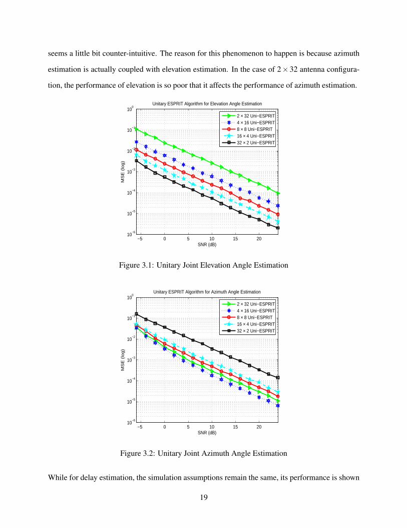
seems a little bit counter-intuitive. The reason for this phenomenon to happen is because azimuth
estimation is actually coupled with elevation estimation. In the case of 2×32 antenna configura-
tion, the performance of elevation is so poor that it affects the performance of azimuth estimation.
−5 0 5 10 15 2010
−6
10−5
10−4
10−3
10−2
10−1
100
SNR (dB)
MS
E (
log
)
Unitary ESPRIT Algorithm for Elevation Angle Estimation
2 × 32 Uni−ESPRIT4 × 16 Uni−ESPRIT8 × 8 Uni−ESPRIT16 × 4 Uni−ESPRIT32 × 2 Uni−ESPRIT
Figure 3.1: Unitary Joint Elevation Angle Estimation
−5 0 5 10 15 2010
−6
10−5
10−4
10−3
10−2
10−1
100
SNR (dB)
MS
E (
log
)
Unitary ESPRIT Algorithm for Azimuth Angle Estimation
2 × 32 Uni−ESPRIT4 × 16 Uni−ESPRIT8 × 8 Uni−ESPRIT16 × 4 Uni−ESPRIT32 × 2 Uni−ESPRIT
Figure 3.2: Unitary Joint Azimuth Angle Estimation
While for delay estimation, the simulation assumptions remain the same, its performance is shown
19
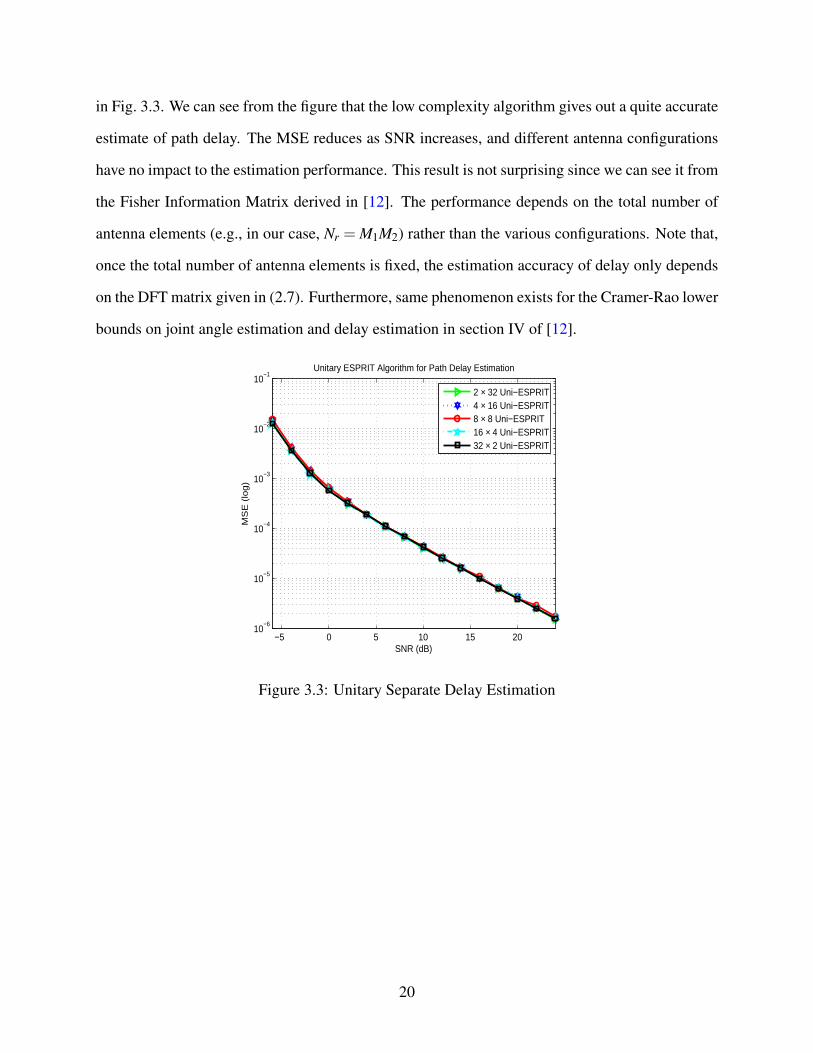
in Fig. 3.3. We can see from the figure that the low complexity algorithm gives out a quite accurate
estimate of path delay. The MSE reduces as SNR increases, and different antenna configurations
have no impact to the estimation performance. This result is not surprising since we can see it from
the Fisher Information Matrix derived in [12]. The performance depends on the total number of
antenna elements (e.g., in our case, Nr = M1M2) rather than the various configurations. Note that,
once the total number of antenna elements is fixed, the estimation accuracy of delay only depends
on the DFT matrix given in (2.7). Furthermore, same phenomenon exists for the Cramer-Rao lower
bounds on joint angle estimation and delay estimation in section IV of [12].
−5 0 5 10 15 2010
−6
10−5
10−4
10−3
10−2
10−1
SNR (dB)
MS
E (
log
)
Unitary ESPRIT Algorithm for Path Delay Estimation
2 × 32 Uni−ESPRIT4 × 16 Uni−ESPRIT8 × 8 Uni−ESPRIT16 × 4 Uni−ESPRIT32 × 2 Uni−ESPRIT
Figure 3.3: Unitary Separate Delay Estimation
20

Chapter 4
Joint Angle and Delay Estimation
In this chapter, we will construct a space-time manifold matrix through stacking data into a
Hankel matrix and jointly estimate the delay and DoAs using 3D ESPRIT-like algorithm. While
for next chapter, a tensor-based system model will come into picture such that an improved signal
subspace estimate is available. Extension to real processing and auto-pairing is straightforward,
and we will illustrate them in section 4.2. Further analysis and simulation results of the estimation
performance are given in section 5.3 in chapter 5.
4.1 Matrix-based Joint Estimation Using Standard ESPRIT
Recall section 2.2 that, the most advantage of JADE is that it can work even when the number
of multi-paths exceeds the number of antennas, as long as the space-time manifold is a tall matrix.
This can be done through constructing a Hankel matrix by left-shifting and stacking M3 copies of
HF to satisfy the requirement [13]. In particular, for a 1 ≤ i ≤ M3, define the left-shifted matrix
HF(i) , HF (:, i:LV−M3+i). (The notation (:, i:LV−M3+i) indicates taking columns i through LV−M3+ i
of a matrix). Then we define the 3D stacked tall channel matrix H, which involves delay, elevation
21

angle and azimuth angle as:
H ,
HF(1)
HF(2)
...
HF(M3)
(Its dimension is M3M1M2×LV −M3 +1)
The reason why we construct the big matrix in this structure is because H has a factorization as
H = ABF, A ,
A
AΨ...
AΨ(M3−1)
= Aψ ⋄A ,
1 1 · · · 1
ψ1 ψ2 · · · ψP
......
......
ψM3−11 ψM3−1
2 · · · ψM3−1P
⋄A
Here, Aψ represents the virtual time delay matrix, and A(τ,θ ,ϕ) = Aψ ⋄A is the space-time man-
ifold matrix. Both Aψ and A are with Vandermonde structure. ⋄ denotes the Khatri-Rao product,
i.e., a column-wise Kronecker product. Note that, the array manifold for elevation angle esti-
mation is different from azimuth angle estimation, whose relationship is transpose of each other,
A(τ,ϕ ,θ) = Aψ ⋄At , where Atℓ = a(uℓ)⊗a(vℓ). If we can choose the stacking parameter w such
that both M3M1M2 ≥ P and LV −M3 + 1 ≥ P are satisfied, and if all factors are full rank, then H
has rank P, which means that we can estimate A up to a P×P factor matrix at the right. Hence,
after proper vectorization and utilization of the shift-invariance property of this highly structured
matrix, we can jointly estimate the unknowns based on standard ESPRIT-like algorithms.
To estimate ψℓ, we should take the first and respectively last M1M2(M3− 1) rows of channel
matrix as two submatrices, while for θℓ estimation, we may take its first and respectively last M1−1
rows for all M3M2 blocks of channel matrix, similarly, for ϕℓ estimation, we may take its first and
respectively last M2−1 rows for all M3M1 blocks. Hence, we can define the selection matrices as
22
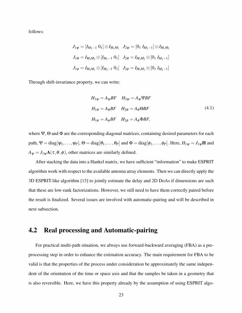
follows:
J1ψ = [IM3−1 01]⊗ IM1M2 J2ψ = [01 IM3−1]⊗ IM1M2
J1θ = IM3M2⊗ [IM1−1 01] J2θ = IM3M2⊗ [01 IM1−1]
J1ϕ = IM3M1⊗ [IM2−1 01] J2ϕ = IM3M1⊗ [01 IM2−1]
Through shift-invariance property, we can write:
H1ψ = AψBF H2ψ = AψΨBF
H1θ = Aθ BF H2θ = Aθ ΘBF
H1ϕ = Aϕ BF H2ϕ = Aϕ ΦBF,
(4.1)
where Ψ, Θ and Φ are the corresponding diagonal matrices, containing desired parameters for each
path, Ψ = diag[ψ1, . . . ,ψP], Θ = diag[θ1, . . . ,θP] and Φ = diag[ϕ1, . . . ,ϕP]. Here, H1ψ = J1ψH and
Aψ = J1ψA(τ,θ ,ϕ), other matrices are similarly defined.
After stacking the data into a Hankel matrix, we have sufficient “information” to make ESPRIT
algorithm work with respect to the available antenna array elements. Then we can directly apply the
3D ESPRIT-like algorithm [15] to jointly estimate the delay and 2D DoAs if dimensions are such
that these are low-rank factorizations. However, we still need to have them correctly paired before
the result is finalized. Several issues are involved with automatic-pairing and will be described in
next subsection.
4.2 Real processing and Automatic-pairing
For practical multi-path situation, we always use forward-backward averaging (FBA) as a pre-
processing step in order to enhance the estimation accuracy. The main requirement for FBA to be
valid is that the properties of the process under consideration be approximately the same indepen-
dent of the orientation of the time or space axis and that the samples be taken in a geometry that
is also reversible. Here, we have this property already by the assumption of using ESPRIT algo-
23

rithm, the antenna array at the base station is centro-symmetric. When FBA is possible, it yields
an effective doubling of the data along with the expected improvements in estimator variances.
Furthermore, in DoA applications, FBA has the desirable effect of reducing correlation between
multi-path coherent signals. Lastly, if FBA is using, the spatial covariance matrix can efficiently
be transformed into a real-valued matrix, which significantly reduces the computational complex-
ity of the subsequent signal subspace estimation step. If such a transformation is used for unitary
ESPRIT, real-valued computations can be maintained for all steps of the algorithm. Actually, FBA
and unitary ESPRIT are naturally integrated.
Hence, for the rest of this section, we will first extend the low complexity Unitary ESPRIT
algorithm to 3D case. Then FBA will be applied. In the end, we will mainly talk about auto-
pairing using joint diagonalization with simultaneous Schur decomposition.
4.2.1 3D extension of Unitary ESPRIT
In section 3.2, we have outlined 2D unitary ESPRIT algorithm for joint elevation and azimuth
angle estimation. Here, we will extend it to 3D case in a similar fashion. By now, we already
have the steering vectors and selection matrices ready. Note that, the third dimension indicating
delay shares the same exponential form as the other two spatial frequencies, described as a(ϖℓ) =
[1,e jψℓ, · · · ,e j(M3−1)ψℓ]T , where ψℓ = e− j 2πL τℓ, ℓ= 1,2, · · · ,P.
Similarly, we need to construct three unitary matrices Qm1,Qm2andQm3 to change the steering
vectors to real values. For elevation, azimuth and delay, the corresponding dimension of upper
sub-matrices are:
m1 = M1M2(M3−1)
m2 = (M1−1)M2M3
m3 = M1(M2−1)M3
24

Assuming m1 = 2q1,m2 = 2q2 and m3 = 2q3 which are all even numbers, we have
Qm1 =1√2
Iq1 jIq1
Πq1 jΠq1
,Qm2 =1√2
Iq2 jIq2
Πq2 jΠq2
,Qm3 =1√2
Iq3 jIq3
Πq3 jΠq3
,Furthermore, the right unitary matrix QNr , where Nr = M1M2M3 , 2M is defined as
QNr =1√2
IM jIM
ΠM jΠM
,As in the 2D case in section 3.2, let us define the transformed steering matrix as AR =QH
NrA. Based
on the three invariance properties of the multi-dimensional steering matrix A, it is straightforward
to get the transformed equation as:
K1ψAR ·Ωψ = K2ψAR
K1θ AR ·Ωθ = K2θ AR
K1ϕ AR ·Ωϕ = K2ϕ AR
(4.2)
where the three corresponding pairs of transformed selection matrices are given by:
K1ψ = 2 ·ReQHm1
J2ψQNr K2ψ = 2 · ImQHm1
J2ψQNr
K1θ = 2 ·ReQHm2
J2θ QNr K2θ = 2 · ImQHm2
J2θ QNr
K1ϕ = 2 ·ReQHm3
J2ϕ QNr K2ϕ = 2 · ImQHm3
J2ϕ QNr
and the three real-valued diagonal matrices
Ωψ , diag
tan(
ϖ1
2
), tan
(ϖ2
2
), . . . , tan
(ϖP
2
)Ωθ , diag
tan(u1
2
), tan
(u2
2
), . . . , tan
(uP
2
)Ωϕ , diag
tan(v1
2
), tan
(v2
2
), . . . , tan
(vP
2
)
25

contain the desired “spatial frequency” information. Till now, all the real-transformation for steer-
ing vectors and construction of selection matrices are complete. In order to keep the SVD of
channel data matrix and all subsequent operations in the real domain, forward-backward averaging
comes into the picture.
4.2.2 Forward-Backward Averaging
Since we are exploiting the specific eigenstructure properties of the sensor array output covari-
ance matrix, it is natural to combine FBA into unitary ESPRIT framework. We use the fact that the
eigenvalues are on the unit circle, along wit the symmetric structures of Aψ , Aθ and Aϕ . Let ΠNr
denote the exchange matrix which reverses the ordering of rows and ΠNc denotes which reverses
the ordering of the columns, and define
HFB = [H ΠNr H ΠNc ]
Here, ¯ indicates complex conjugate. In our later simulation, we set the number of paths P to two
since forward-backward averaging can only resolve up to two paths. If we want to resolve more
paths, spatial smoothing technique should be taken into account. Spatial smoothing pre-processing
step leads to a decorrelation of the paths and an increase in the number of available snapshots. The
key idea is that we divide the array into a number of identical displaced sub-arrays and average the
spatial covariance matrix over these sub-arrays. Consequently, array aperture is sacriced. Haardt
et al. [16] already incorporated spatial smoothing technique to unitary ESPRIT both in matrix and
tensor form, more details can be seen in section VI of [16].
Then we multiply unitary matrices on both sides of HFB to transform the complex-valued data
matrix into real-valued domain.
HH = QNr HFB QNN (Its Dimension: M1M2M3×NN)
26
where we assume NN = 2Nc = 2(LV −1) and
QNN =1√2
INc jINc
ΠNc jΠNc
,Similarly, we have Us ∈ RM1M2M3×P the signal subspace from a real-valued SVD of HH and
T be the linear nonsingular transformation matrix (whose dimension is P×P). Since the signal
subspace and the real-valued steering matrix AR spans the same P− dimensional subspace asymp-
totically or under the case of no additive noise, we have Us ≈ ART . Substituting this relation
into (4.2), we have three real-valued invariance equations:
K1ψUs ·ϒψ = K2ψUs
K1θUs ·ϒθ = K2θUs
K1ϕUs ·ϒϕ = K2ϕUs
(4.3)
where ϒψ , T−1ΩψT , ϒθ , T−1Ωθ T and ϒϕ , T−1Ωϕ T . Here, the three real-valued matrices
ϒψ , ϒθ and ϒϕ are related with the diagonal matrices via eigenvalue preserving similarity trans-
formations. Moreover, they share the same set of eigenvectors T in the noiseless case or with an
infinite number of experiments. The problem now is if these eigenvalue solutions were calculated
independently via LS, TLS or SLS, it would be quite difficult to pair the resulting three distinct sets
of spatial frequency estimates. An easy way to make sure automatic pairing is to find the matrix of
eigenvectors T the same for all three dimensions.
However, in practice, we only have a finite number of noise-corrupted snapshots. Therefore,
the three real-valued matrices ϒψ , ϒθ and ϒϕ do not exactly share the same set of eigenvectors.
If we just choose one dimension to determine the set of common eigenvectors, the solution will
rely on this specific choice and discard information contained in other two matrices. Obviously,
it is not the best option. Thus, from a statistical point of view, it is desirable, for the sake of
accuracy and robustness, to compute the “average eigenstructure” of these three matrices. In the 2D
27

case, we solve this problem by a trick, which is to calculate the eigenvalues of the “complexified”
matrix ϒx + jϒy ∈ CP×P, kind of averaging. Therefore, automatic pairing of the eigenvalues can
be achieved. However, for 3D case, this trick doesn’t work anymore and we develop a Jacobi-type
method to calculate an SSD of several nonsymmetric matrices. Note that, this method also extends
to multi-dimensional case.
4.2.3 Joint diagonalization
Recall that the real eigenvalues of real-valued nonsymmetric matrices can efficiently be com-
puted through an eigenvalue revealing real Schur decomposition. In the noiseless case or with an
infinite number of experiments, the SSD of the three matrices ϒψ , ϒθ and ϒϕ yields three real-
valued upper triangular matrices that exhibit the automatically paired eigenvalues on their main
diagonals. Under the assumption of additive noise and a finite number of experiments, an or-
thogonal similarity transformation might not be able to produce three upper triangular matrices
simultaneously, since the three noisy matrices do not share a common set of eigenvectors. In this
case, the resulting matrices should be “almost” upper triangular in a least square sense, i.e., an
approximate simultaneous upper triangularization that reveals the “average eigenstructure” should
be calculated.
Hence, in least square sense, we want to minimize some cost function with respect to lower
triangular part of matrices going to zero. An efficient Jacobi-type technique to achieve such an ap-
proximate simultaneous diagonalization is presented in [17] for symmetric matrices and its mod-
ified version for nonsymmetric matrices is proposed in [18]. The details are in [17] and [18] and
need not be repeated here. The cost function is given as:
C(O) = ||L(OT ϒψ O)||2F + ||L(OT ϒθ O)||2F + ||L(OT ϒϕ O)||2F
over the set of orthogonal matrices O ∈Rp×P that can be written as products of elementary Jacobi
rotations. || · ||F denotes the Frobenius-norm. L(·) is defined as an operation that extracts the
28

strictly lower triangular part and the elements on the main diagonal to zero.
In Jacobi-type algorithms, the orthogonal matrixO is decomposed into a product of elementary
Jacobi rotations
Oqp =
1 · · · 0 · · · 0 · · · 0... . . . ...
......
0 · · · c · · · s · · · 0...
... . . . ......
0 · · · −s · · · c · · · 0...
...... . . . ...
0 · · · 0 · · · 0 · · · 1
such that
O = ∏# of sweeps
P
∏q=1
q−1
∏p=1Oqp
Here, Jacobi rotations Oqp are defined as orthogonal matrices where all diagonal elements are one
except for the two elements c in rows (and columns) p and q. Likewise, all off-diagonal elements
of Oqp are zero except for the two elements s and −s. The real numbers c = cosϑ and s = sinϑ
are the cosine and sine of a rotation angle ϑ such that c2 + s2 = 1. We are developing an iterative
procedure to find a particular rotation angle ϑ such that the cost function is minimized, namely the
number of sweeps. Then, c and s is obtained and we can have our desired orthogonal matrix O. In
this case, ϒψ , ϒθ and ϒϕ can be effectively transformed to diagonal matrices simultaneously, thus
the challenge of automatic pairing in joint estimation problem is solved.
29

Algorithm 1: Three-Dimensional Unitary ESPRIT OutlineInput : Extended data matrix after Hankel constructing and forward-backward averagingOutput: Desired joint estimate of 3D parametersbegin
I. Real processing:HH = QNr HFB QNN
II. Compute the signal subspace estimate Us as the P dominant left singular vectors ofextended data matrix HH (square-root approach)III. Solve the set of invariance equations by means of LS, TLS or SLS.
K1ψUs ·ϒψ = K2ψUs
K1θUs ·ϒθ = K2θUs
K1ϕUs ·ϒϕ = K2ϕUs
IV. Joint frequency estimation by computing the SSD of the real-valued P×P matrices
Uψ =OT ϒψ OUθ =OT ϒθ OUϕ =OT ϒϕ O
V. “Average eigenstructure” should be calculated and the desired 3D parameter jointestimation are obtained
end
30

Chapter 5
Tensor-based JADE Using ESPRIT
For high order harmonic retrieval problems, since the measurement data is multi-dimensional,
current approaches require stacking the dimensions into one highly structured matrix. However,
in the conventional subspace estimation step, this stacked data model cannot exploit the essential
structure of the original received signal. Thus in this chapter, we introduce tensor, which can be
used to store and manipulate high order data in their native multi-dimensional form, to estimate the
signal subspace through a high order SVD. This will lead to a better estimate performance because
of the improved signal subspace estimate. Furthermore, this new concept and system model can be
applied to any multi-dimensional subspace-based parameter estimation scheme. It can be regarded
as a whole framework for multi-dimensional harmonic retrieval problems.
5.1 Basic tensor notation and operation
Tensors provide a natural and concise mathematical framework for formulating and solving
problems in more and more research areas. They are geometric objects that describe linear relations
between scalars, vectors, matrices and other tensors. The order (also degree) of a tensor is the
dimensionality of the array needed to represent it, or equivalently, the number of indices needed
to label a component of that array. For example, the (i, j,k) element of a third-order tensor B as
bi, j,k. An n-mode vector of an I1× I2×·· ·× IN-dimensional tensor B is an In-dimensional vector
31

obtained from B by varying the index in and keeping the other indices fixed. Moreover, a matrix
unfolding of the tensor B along the n-th mode is denoted by [B](n) and can be understood as a
matrix containing all the n-mode vectors of tensor B. We also define the concatenation of two
tensors along the n-th mode via the operator [A⊔n B]. The order of the columns is chosen in
accordance with [19], and the following tensor operations we use are also consistent with [19].
• The outer product of the tensor A ∈ CI1×I2×···×IN and B ∈ CJ1×J2×···×JM is given by
C =AB ∈ CI1×I2×···×IN×J1×J2×···×JM
ci1,i2,...,iN , j1, j2,..., jM = ai1,i2,...,iN ·b j1, j2,..., jM
In other words, the tensor C contains all possible combinations of pairwise products between
the elements of A and B. This operator is very closely related to the Kronecker product
defined for matrices.
• The n-mode product of a tensor A ∈ CI1×I2×···×IN and a matrix U ∈ CJn×In along the n-th
mode is denoted as
B =A×n U ∈ CI1×I2×···×In−1×Jn×In+1×···×IN
bi1,i2,...,in−1, jn,in+1,...,iN =In
∑in=1
ai1,i2,...,iN ·u jn,in .
It may be visualized by multiplying all n-mode vectors of A from the left-hand side by the
matrix U .
• The higher-order SVD (HOSVD) of a tensor A ∈ CI1×I2×···×IN is given by
A= S ×1 U1×2 U2 · · ·×N UN
where S ∈CI1×I2×···×IN is the core tensor which satisfies the all-orthogonality conditions and
Un ∈ CIn×In,n = 1,2, . . . ,N are the unitary matrices of n-mode singular vectors.
32

5.2 Tensor-based Joint Estimation Using Standard ESPRIT
Starting from H, the multi-dimensional channel data after Hankel constructing , we need to
represent it in its tensor form rather than stacking it into a highly structured matrix. The original
measurement samples are given by:
hm1,m2,m3,m4 =P
∑ℓ=1
αℓe− j(m1−1)uℓ · e− j(m2−1)vℓ·
e− j(m3−1)ϖℓ · e− j(m4−1)ϖℓ +dm1,m2,m3,m4
where m1 = 1,2, . . . ,M1,m2 = 1,2, . . . ,M2,m3 = 1,2, . . . ,M3 and m4 = 1,2, . . . ,LV −1. For nota-
tion simplicity, we denote N = LV − 1 because LV − 1 is the number of time domain samples of
the known pulse shape function. dm1,m2,m3,m4 represents the zero mean additive noise component
inherent in the measurement process.
In order to arrive at a more compressed formulation of the data model, we collect all the samples
hm1,m2,m3,m4 into one multi-dimensional array (MDA). Specifically, let xℓ = αℓ, the 4-dimensional
channel estimatesH can be expressed as:
H=A×4 XT +D. (5.1)
Here, X is the P×N vectorized matrix of attenuated amplitude. H ∈ CM1×M2×M3×N denotes all
estimated impulse response samples, while D ∈ CM1×M2×M3×N collects all the estimation noise
samples. A ∈ CM1×M2×M3×P is referred to as the array steering tensor, which can be expressed as
A = I4,P ×1A(1)×2A(2)
×3A(3), I4,P is the defined rank-4 identity tensor with each mode a P×P
identity matrix. The array response matrices in each mode are shown to be:
A(1) = [a(u1),a(u2), . . . ,a(uP)]
A(2) = [a(v1),a(v2), . . . ,a(vP)]
A(3) = [a(ϖ1),a(ϖ2), . . . ,a(ϖP)]
33

Since we have the identity relationship between matrix and tensor, e.g., A = [A]T(R+1), which
means the matrix is equal to the transpose of the unfolding of the measurement tensor along the
last dimension. The tensor-based data model can be equivalently transformed to the matrix-based
data model in frequency domain. Most approaches and results obtained from matrix point of view
are ready to apply for the tensor case.
For now, We apply FBA and the following real-valued subspace estimation steps are naturally
extended to the tensor case. Concepts and principles of FBA have already been introduced in
chapter 4, thus we just write out the tensor version of FBA:
Hfba = [H ⊔4 (H∗×1 ΠM1 ×2ΠM2 ×3ΠM3 ×4ΠN)]
Note that, the FBA tensor Hfba for each measurement tensor is centro-Hermitian, which possess a
bunch of good properties for analytical assessment. The centro-Hermitian tensor is the extension
of centro-Hermitian matrix, which can be transformed into real-valued tensor by n-mode product
with unitary matrices. It is at this point that unitary ESPRIT comes into picture.
Similarly, recall section 3.2, we need to construct three unitary matrices QM1 ,QM2 and QM3
corresponding to the delay, elevation and azimuth array steering vector. Assuming M1 = 2Q1,M2 =
2Q2 and M3 = 2Q3 which are all even numbers, we have
QM1 =1√2
IQ1 jIQ1
ΠQ1 jΠQ1
QM2 =1√2
IQ2 jIQ2
ΠQ2 jΠQ2
QM3 =1√2
IQ3 jIQ3
ΠQ3 jΠQ3
.
34

Furthermore, we define the left Π-real unitary matrices of odd order as:
QM′1=
1√2
IQ′1
0Q′1×1 jIQ′1
01×Q′1
√2 01×Q′1
ΠQ′10Q′1×1 jΠQ′1
QM′2=
1√2
IQ′2
0Q′2×1 jIQ′2
01×Q′2
√2 01×Q′2
ΠQ′20Q′2×1 jΠQ′2
QM′3=
1√2
IQ′3
0Q′3×1 jIQ′3
01×Q′3
√2 01×Q′3
ΠQ′30Q′3×1 jΠQ′3
,
where Q′1 = (M1−1)/2, Q
′2 = (M2−1)/2 and Q
′3 = (M3−1)/2.
Before utilizing any subspace-based parameter estimation scheme, we need to estimate a basis
for the multi-dimensional signal subspace from the noisy observations. Similarly, the tensor-based
signal subspace estimation can be achieved through a truncated higher-order singular value decom-
position (HOSVD) ofHfba [16]:
Hfba ≈ S ×1U1 ×2U2 ×3U3 ×4U4 (5.2)
where S ∈ C p1×p2×p3×N is the truncated core tensor and Ur ∈ CMr×pr for r = 1,2,3 , U4 ∈ CP×N are
the matrices of dominant r-mode singular vectors. pr represents the rank of r-mode singular matrix
unfolding. Actually, the HOSVD is computed through SVDs of the unfoldings. Based on (5.2), a
tensor-based subspace estimate can be written as:
U [s] ≈ S ×1U [s]1 ×2U [s]
2 ×3U [s]3 ×4U [s]
4(5.3)
It is already shown in [16] that, an improved signal subspace estimate is achieved using tensor-
based HOSVD in the presence of noise and if the number of paths is strictly less than the number
of array elements in at least one of the modes. This is because the tensor approach allows us to
filter out noise in each of the modes of estimated signal subspace separately which results in an
35
improved signal subspace. We can see this improvement more clearly through the performance
comparison with matrix-based method in subsection 5.3.2.
Assume the 3D array steering tensor features shift-invariance in each of its modes, we can di-
rectly apply multi-dimensional standard ESPRIT algorithm to write the shift-invariance equations
as:
A×1J(1)1 ×4Θ =A×1J(1)2
A×2J(2)1 ×4Φ =A×2J(2)2
A×3J(3)1 ×4Ψ =A×3J(3)2
(5.4)
where Θ, Φ and Ψ are already defined in matrix-based subsection. J(r)i ∈ R(Mr−1)×Mr , i = 1,2
represent the selection matrices for the rth mode under maximum overlapping.
J(r)1 = [IMr−1 0(Mr−1)×1]
J(r)2 = [0(Mr−1) ×1IMr−1];
Since the array steering tensor approximately span the same vector space as the estimated signal
subspace U [s] similar to the matrix case:
A≈ U [s]×4T
for some P×P nonsingular transform matrix T . We may substitute the above relation back to (5.4):
U [s]×1J(1)1 ×4Θ≈ U [s]
×1J(1)2
U [s]×2J(2)1 ×4Φ≈ U [s]
×2J(2)2
U [s]×3J(3)1 ×4Ψ≈ U [s]
×3J(3)2
In case of unitary ESPRIT, the selection matrices need to be updated a little bit using the unitary
36

matrices we have defined above.
K1ψU [s] ·ϒψ = K2ψU [s]
K1θU [s] ·ϒθ = K2θU [s]
K1ϕU [s] ·ϒϕ = K2ϕU [s]
(5.5)
where the three corresponding pairs of transformed selection matrices are given by:
K1ψ = 2 ·ReQHM′1
J(1)2 QM1 K2ψ = 2 · ImQHM′1
J(1)2 QM1
K1θ = 2 ·ReQHM′2
J(2)2 QM2 K2θ = 2 · ImQHM′2
J(2)2 QM2
K1ϕ = 2 ·ReQHM′3
J(3)2 QM3 K2ϕ = 2 · ImQHM′3
J(3)2 QM3
As before, equation (5.5) represents a tensor least squares problem, and the solution is given by:
ϒTψ =
(ˆK1ψ ·[U [s]]T
4
)†
· ˆK2ψ ·[U [s]]T
4
ϒTθ =
(ˆK1θ ·[U [s]]T
4
)†
· ˆK2θ ·[U [s]]T
4
ϒTϕ =
(ˆK1ϕ ·[U [s]]T
4
)†
· ˆK2ϕ ·[U [s]]T
4
where
ˆK1ψ = K1ψ ⊗ IM1M2ˆK2ψ = K2ψ ⊗ IM1M2
ˆK1θ = IM3M2⊗K1θ ˆK2θ = IM3M2⊗K2θ
ˆK1ϕ = IM3M1⊗K1ϕ ˆK2ϕ = IM3M1⊗K2ϕ
The HOSVD-based subspace estimate[U [s]]T
4defined in (5.3) is linked to the SVD-based subspace
estimate Us via the following algebraic relation:
[U [s]]T
4= (T1⊗ T2⊗ T3) ·Us
37

where Tr ∈CMr×Mr represent estimates of the projection matrices onto the r-modes of measurement
tensor, which are computed via Tr =ˆ
U [s]r
ˆU [s]
r
H.
The final step of the 3-D unitary ESPRIT algorithm is still the SSD operation, to make different
modes of measurement tensor share the same set of eigenvectors. This guarantees the correct
pairing of the paths over modes. The idea is exactly the same with matrix-based ESPRIT algorithm,
so it is unnecessary to write out again.
5.3 Matrix and Tensor-based Unitary ESPRIT Algorithm Sim-
ulation
In this section, we evaluate both matrix-based and tensor-based joint estimation algorithm un-
der various antenna configurations, to see the impact of practical implementation on estimation
performance. Assume it is a two paths situation with DoAs [70,77] for elevation and [45,60] for
azimuth, path fading amplitudes [1,0.8] and time delay [0.5,2.1]s, same as 2D joint angle estima-
tion scenario. Additionally, we set the stacking number of Hankel construction to be 2. The number
of sweeps in SSD operation is determined as 10. All the results are based on 1000 Monte-Carlo
runs under SNR ranging form 6 dB to 24 dB. Here, the definition of SNR is the signal to noise
ratio for the channel, which is impacted by the multi-paths effect. Originally, the signal power is
always assumed to be 1 after normalization, but for our two paths scenario (one main path, one
off-main path), the signal power should be the sum of these two paths’ signal power. We will first
compare the estimation performance between separate 2D joint angle and delay estimation with
matrix-based 3D JADE. Then the comparison between matrix and tensor-based 3D JADE follow
up.
38

5.3.1 Comparison between 2D Joint Angle Estimation and Matrix-based 3D
JADE Estimation
For delay estimation, we can see that different antenna configurations don’t have much impact
on the estimation performance, as shown in Fig. 5.1(a) and Fig. 5.1(b). We found that this result
is not surprising since we can see it from the Fisher Information Matrix derived in [12]. The
performance depends on the total number of antenna elements (e.g., in our case, Nr = M1M2M3)
rather than the various configurations. Note that, once the total number of antenna elements is
fixed, the estimation accuracy of delay only depends on the DFT matrix given in (2.7).
6 8 10 12 14 16 18 20 22 2410
−6
10−5
10−4
10−3
SNR (dB)
MS
E (
log
)
Unitary ESPRIT Algorithm for Path Delay Estimation
2 × 32 Uni−ESPRIT4 × 16 Uni−ESPRIT8 × 8 Uni−ESPRIT16 × 4 Uni−ESPRIT32 × 2 Uni−ESPRIT
(a)
6 8 10 12 14 16 18 20 22 2410
−0.3
10−0.2
10−0.1
SNR (dB)
MS
E (
log
)
3D Matrix−based JADE Unitary ESPRIT Algorithm for Delay Estimation
2 × 32 Uni−ESPRIT4 × 16 Uni−ESPRIT8 × 8 Uni−ESPRIT16 × 4 Uni−ESPRIT32 × 2 Uni−ESPRIT
(b)
Figure 5.1: Comparison Between 2D Separate and 3D Matrix-based Joint Delay Estimation
Fig. 5.2(a) and Fig. 5.2(b) shows that, for elevation angle estimation, its performance is pro-
portional to the number of antennas vertically. This matches with our conventional understanding
because for 1D antenna array, a larger number of antenna elements will contribute to a better per-
formance intuitively. Moreover, we may compare the trend of Fig. 5.2(b) with Fig. 5.2(a) to obtain
that, the elevation angle estimation is actually impacted by the delay estimation through this joint
algorithm. In low SNR regime, even a 32× 2 antenna configuration doesn’t contribute much to
the elevation estimation performance, only when we operate in high SNR regime, the advantage
of more antennas will exhibit. Another point is that, as CRLB suggests, the more parameters we
are trying to estimate, the more uncertainty will be involved. Hence, for any of these configura-
39

tions, the MSEs of 3D JADE joint elevation estimation is much higher than those of 2D joint angle
estimation, e.g., more than a magnitude of order.
6 8 10 12 14 16 18 20 22 2410
−6
10−5
10−4
10−3
10−2
SNR (dB)
MS
E (
log
)
Unitary ESPRIT Algorithm for Elevation Angle Estimation
2 × 32 Uni−ESPRIT4 × 16 Uni−ESPRIT8 × 8 Uni−ESPRIT16 × 4 Uni−ESPRIT32 × 2 Uni−ESPRIT
(a)
6 8 10 12 14 16 18 20 22 2410
−2
10−1
100
101
SNR (dB)
MS
E (
log
)
3D Matrix−based JADE Unitary ESPRIT Algorithm for Elevation Angle Estimation
2 × 32 Uni−ESPRIT4 × 16 Uni−ESPRIT8 × 8 Uni−ESPRIT16 × 4 Uni−ESPRIT32 × 2 Uni−ESPRIT
(b)
Figure 5.2: Comparison Between 2D Joint and 3D Matrix-based Joint Elevation Angle Estimation
Another interesting finding of joint azimuth angle estimation is illustrated in Fig. 5.3(a) and
Fig. 5.3(b). We can see that a 4× 16 configuration gives out a better performance than 2× 32.
The result is similar to our former observation in [12] and has been analyzed analytically in [20].
This means, for joint estimation of three parameters, we can still get the fact that, azimuth angle
estimation is indeed affected by the estimation performance of elevation angle. In the case of the
2×32 array, the performance of elevation estimation is so poor that it affects the performance of
azimuth estimation. We can also observe that in the low SNR regime, all curves merges together.
This is because when SNR is too low, we can’t get accurate estimate for θ , ϕ and τ , no matter for
what kind of antenna configurations. As the SNR increases, the impact of antenna configuration
comes into the picture as shown in Fig. 5.3(b).
Though 3D joint estimation scheme give out much worse estimation performance than separate
estimation, we need to make sure that they are automatically correct-pairing. As 3D algorithm
exhibits, joint estimation will give out a better resolution than the separate ones. This is due to the
fact that the ESPRIT-like algorithm takes advantage of all the information of received signals from
all the antenna elements. And now, we can resolve a larger number of rays in cases where two or
more rays have equal DoAs or delays.
40
6 8 10 12 14 16 18 20 22 24
10−5
10−4
10−3
10−2
SNR (dB)
MS
E (
log
)
Unitary ESPRIT Algorithm for Azimuth Angle Estimation
2 × 32 Uni−ESPRIT4 × 16 Uni−ESPRIT8 × 8 Uni−ESPRIT16 × 4 Uni−ESPRIT32 × 2 Uni−ESPRIT
(a)
6 8 10 12 14 16 18 20 22 2410
−1
100
101
SNR (dB)
MS
E (
log
)
3D Matrix−based JADE Unitary ESPRIT Algorithm for Azimuth Angle Estimation
2 × 32 Uni−ESPRIT4 × 16 Uni−ESPRIT8 × 8 Uni−ESPRIT16 × 4 Uni−ESPRIT32 × 2 Uni−ESPRIT
(b)
Figure 5.3: Comparison Between 2D Joint and 3D Matrix-based Joint Azimuth Angle Estimation
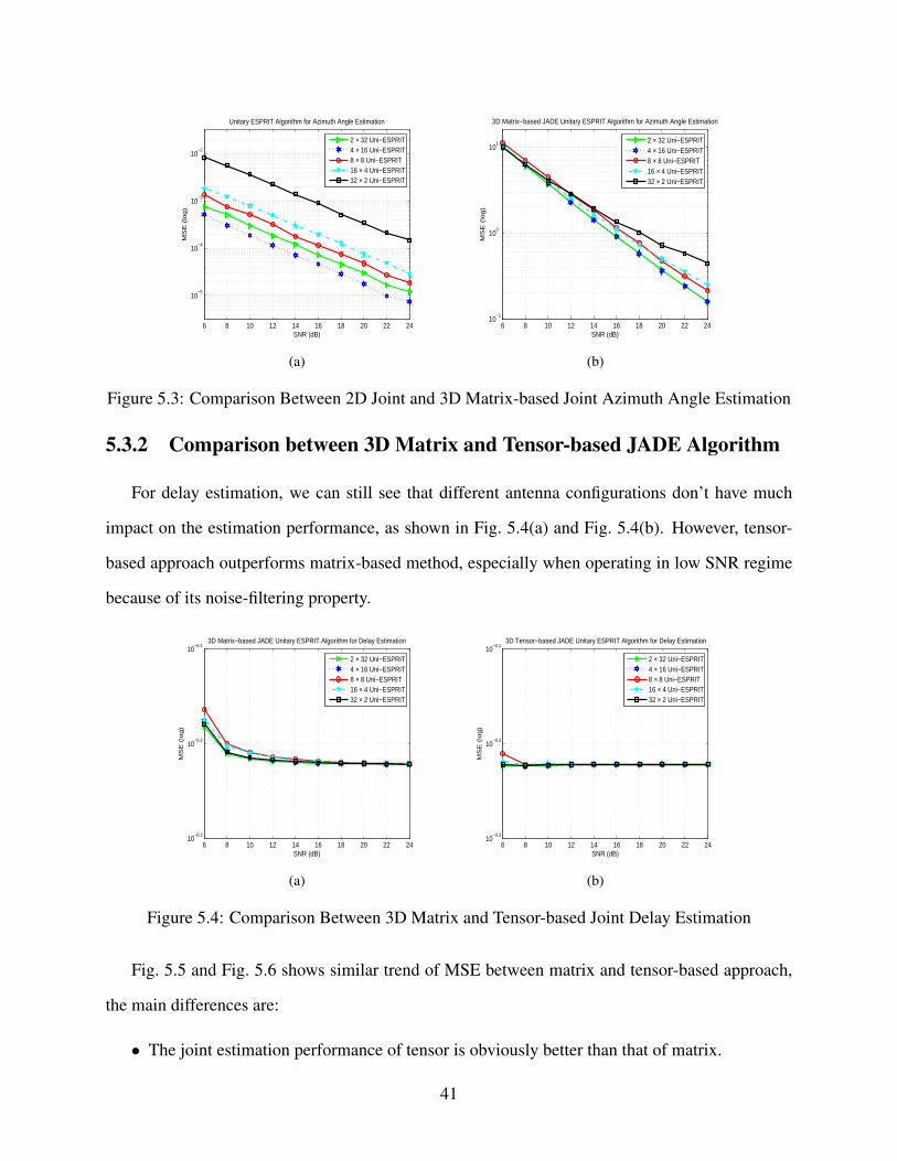
5.3.2 Comparison between 3D Matrix and Tensor-based JADE Algorithm
For delay estimation, we can still see that different antenna configurations don’t have much
impact on the estimation performance, as shown in Fig. 5.4(a) and Fig. 5.4(b). However, tensor-
based approach outperforms matrix-based method, especially when operating in low SNR regime
because of its noise-filtering property.
6 8 10 12 14 16 18 20 22 2410
−0.3
10−0.2
10−0.1
SNR (dB)
MS
E (
log
)
3D Matrix−based JADE Unitary ESPRIT Algorithm for Delay Estimation
2 × 32 Uni−ESPRIT4 × 16 Uni−ESPRIT8 × 8 Uni−ESPRIT16 × 4 Uni−ESPRIT32 × 2 Uni−ESPRIT
(a)
6 8 10 12 14 16 18 20 22 2410
−0.3
10−0.2
10−0.1
SNR (dB)
MS
E (
log
)
3D Tensor−based JADE Unitary ESPRIT Algorithm for Delay Estimation
2 × 32 Uni−ESPRIT4 × 16 Uni−ESPRIT8 × 8 Uni−ESPRIT16 × 4 Uni−ESPRIT32 × 2 Uni−ESPRIT
(b)
Figure 5.4: Comparison Between 3D Matrix and Tensor-based Joint Delay Estimation
Fig. 5.5 and Fig. 5.6 shows similar trend of MSE between matrix and tensor-based approach,
the main differences are:
• The joint estimation performance of tensor is obviously better than that of matrix.
41

• Fig. 5.5(b) and Fig. 5.6(b) look more separate. But in Fig. 5.5(a) and Fig. 5.6(a), especially
in low SNR regime, curves are overlapping because they are effected by each other if using
matrix-based joint estimation scheme.
• For tensor-based elevation angle estimation in low SNR regime, a 16× 4 configuration is
better than that of 32×2 configuration, which is different from matrix-based results.
As we know, tensor restores the multi-dimensional data in its natural structure, which can be re-
garded as separate processing. It allows us to filter out noise in each of the modes of estimated
signal subspace separately which results in an improved signal subspace. Another point is, we
always focus on azimuth angle estimation is because, for a fixed number of total antenna elements,
the azimuth angle estimation is more crucial for MIMO beam-forming in cellular systems. For
tensor-based approach, we observe again the fact that a 4×16 configuration is better than that of
2×32 configuration. Combined with our simulation and analytical results, we may say that a more
symmetrical structure leads to a relatively smaller MSE.
6 8 10 12 14 16 18 20 22 2410
−2
10−1
100
101
SNR (dB)
MS
E (
log
)
3D Matrix−based JADE Unitary ESPRIT Algorithm for Elevation Angle Estimation
2 × 32 Uni−ESPRIT4 × 16 Uni−ESPRIT8 × 8 Uni−ESPRIT16 × 4 Uni−ESPRIT32 × 2 Uni−ESPRIT
(a)
6 8 10 12 14 16 18 20 22 2410
−2
10−1
100
101
SNR (dB)
MS
E (
log
)
3D Tensor−based JADE Unitary ESPRIT Algorithm for Elevation Angle Estimation
2 × 32 Uni−ESPRIT4 × 16 Uni−ESPRIT8 × 8 Uni−ESPRIT16 × 4 Uni−ESPRIT32 × 2 Uni−ESPRIT
(b)
Figure 5.5: Comparison Between 3D Matrix and Tensor-based Joint Elevation Angle Estimation
Therefore, the tensor-based approach gives out a even better performance as compared in
Fig. 5.4, Fig. 5.5 and Fig. 5.6. We can see that almost a half magnitude of order improvement
is obtained for all three parameter estimation.
42
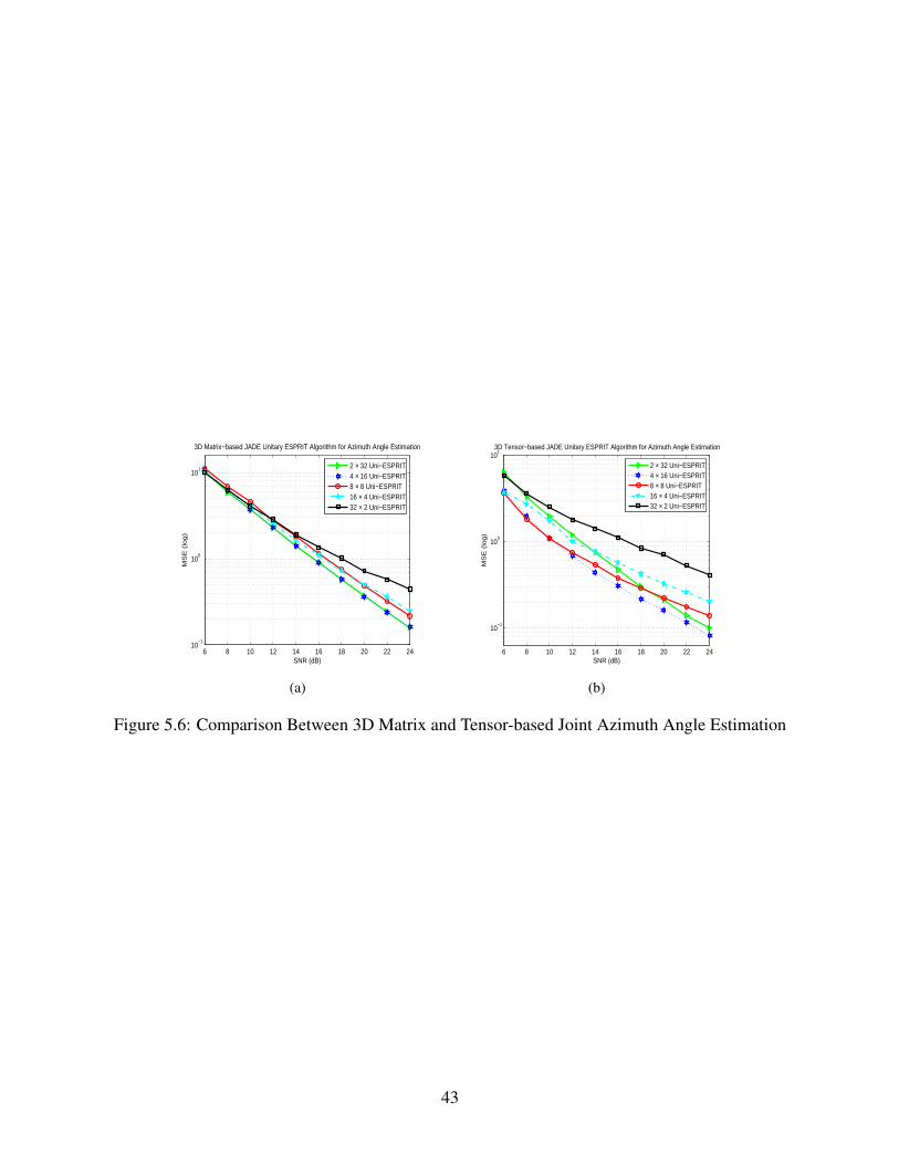
6 8 10 12 14 16 18 20 22 2410
−1
100
101
SNR (dB)
MS
E (
log
)
3D Matrix−based JADE Unitary ESPRIT Algorithm for Azimuth Angle Estimation
2 × 32 Uni−ESPRIT4 × 16 Uni−ESPRIT8 × 8 Uni−ESPRIT16 × 4 Uni−ESPRIT32 × 2 Uni−ESPRIT
(a)
6 8 10 12 14 16 18 20 22 24
10−1
100
101
SNR (dB)
MS
E (
log
)
3D Tensor−based JADE Unitary ESPRIT Algorithm for Azimuth Angle Estimation
2 × 32 Uni−ESPRIT4 × 16 Uni−ESPRIT8 × 8 Uni−ESPRIT16 × 4 Uni−ESPRIT32 × 2 Uni−ESPRIT
(b)
Figure 5.6: Comparison Between 3D Matrix and Tensor-based Joint Azimuth Angle Estimation
43

Chapter 6
Conclusion and Future Work
The thesis illustrates the application of DoA estimation technique (ESPRIT algorithm) to a 2D
Massive MIMO broadband communication regime and jointly estimate the 3D channel parameters:
elevation angle, azimuth angle and path delay, which is crucial for downlink digital beamforming
in cellular networks. The fundamental assumption is that antenna array at the base station should
possess some particular structures, e.g., if it can be divided into two same sub-arrays.
ESPRIT algorithm uses the relationship between eigenspace of two divided array output ma-
trices to obtain our desired parameters, and the complexity is very promising compared to MUSIC
and MLE. Since multi-dimensional MUSIC and MLE approach both need a search along the whole
multi-dimensional space, while ESPRIT works well without the exhaustive search. The linearity
property between signal subspace and array manifold, and the invariance property between two
sub-arrays highlight the advantage of ESPRIT, since multi-dimensional extension, real processing,
joint diagonalization, forward-backward averaging etc. are easily incorporated compared to other
DoA estimation approaches.
We observe that azimuth angle estimation actually couples with elevation angle estimation.
In circumstances where elevation angle estimation performance is so poor, it affects our azimuth
performance. Furthermore, different antenna configurations will contribute to different estimation
performance, as well as capacity loss. In general, a more symmetrical antenna configuration leads
44

to a relatively better estimation performance as for the design of antenna arrays at the base station.
The last thing to note is that various antenna configurations don’t have much impact to path delay
estimation as long as the total number of antenna array elements is fixed. It only depends on the
DFT matrix, or simply the number of snapshots when you sample the known pulse shape function.
Improved results could be obtained by the application of tensor processing. Tensor is a pow-
erful geometric tool and widely used in signal processing and wireless communication area [10].
It helps us store, retrieve, process the measurement data in its original form, and separate mode
processing can effectively filter out the noise compared to matrix-based methods. More impor-
tantly, tensor processing will give us a better signal subspace estimate, which is beneficial for
all subspace-based estimation algorithms. It is a whole new framework rather than just a simple
preprocessing step.
There are still many aspects we can investigate in the future, e.g., large scale MIMO, multi-user
scenario, other DoA estimation techniques with multi-dimensional extension, how training will
affect the estimation performance within OFDM, correct pairing between different sub-carriers if
one user can be supplied with more than one sub-carrier and analytical assessment in multi-path,
multi-user case, etc.
• When large scale MIMO is involved, many results obtained before are no longer valid be-
cause random matrix theory kicks in. Only asymptotic behaviour is shown by now [21, 22],
but no practical implementation is there. Samsung is developing a Full Dimension MIMO
(FD-MIMO) [6] technology in the context of next generation evolution towards B4G and
5G cellular systems, which relies on the 2D base station antenna array. Even they analyze
the system performance asymptotically, the prototype is still quite small comparing to the
MIMO definition, a 32×64 2D antenna array.
• Giuseppe Caire propose Joint Spatial Division and Multiplexing (JSDM) in [23] , an ap-
proach to multi-user MIMO downlink that exploits the structure of the correlation of the
channel vectors in order to allow for a large number of antennas at the base station while
requiring reduced-dimensional Channel State Information at the Transmitter (CSIT). Two
45

dimensional base station antenna array, DFT-based pre-beamforming, random matrix the-
ory, fairness criteria are all involved.
• In [24], A. Lee and Thomas compares the most popular DoA estimation techniques with
their multi-dimensional extensions in great detail, and showed us that MD-MLE outper-
forms all algorithms with respect to MSE, except for its high computational cost. And one-
dimensional MUSIC outperforms all of the MD algorithms for random angle-independent
array perturbations. Hence for different applications, we may consider MUSIC or MLE
instead of ESPRIT from time to time.
• In our paper, we assume that the channel frequency response estimate is available. However,
in practical situation, it is quite hard to get the estimate even we use the training sequence.
Furthermore, how much training is proper is another interesting topic to look at [25]. Pilot
contamination is also severe and has great impact to channel estimation performance when
we are in multi-cell system [26].
• Closed-form results can give us more intuition and theoretically confirm the simulated ob-
servations we had made. In [27], Haardt et al. already show the derivation of closed-form
MSE expressions using tensor-based multi-dimensional Unitary ESPRIT algorithm, in sin-
gle source case. Equivalently in our situation, only the single path problem is analytically
assessed. Multi-path and multi-user results are surely helpful if derived as benchmark.
Therefore, this paper lays a good foundation for further analysis and test on future design of prac-
tical broadband MIMO-OFDM wireless communication system.
46

Part II
Analysis of Direction of Arrival Estimation
Algorithms for Basal Ice Sheet Tomography
47

Chapter 7
Introduction
Scientific research indicates the current sea level rise is about 3.5 mm per year worldwide.
According to the US National Oceanic and Atmospheric Administration (NOAA) [28], this is
a significantly larger rate than the sea level rise averaged over the last several thousand years,
and the rate may be increasing. This trend puts thousands of coastal cities, islands and natural
environments at risk in the future. The rise in sea level is contributed through two major factors:
one is thermal expansion, the other is the melting of glaciers and polar ice sheets. The latter of
which is the primary interest of this work. Analysis of the geological record suggests there is ice
loss in Greenland and West Antarctica due to global warming. To have knowledge of the current
ice mass balance and to predict ice sheet dynamics in these two regions, we need to know the ice
sheet thickness and the physical properties of the ice sheet surface and bed. In this regard, we
require the estimation of basal ice sheet topography at fine resolution and over extensive portions
of the polar ice sheets.
There are several methods that can be used to observe the basal conditions of an ice sheet
as discussed in [29]. The most direct way is drilling a borehole to the bottom of the ice sheet
and passing the measurement equipment down into the borehole. However, wide area coverage
with fine resolution is infeasible. Similarly, seismic studies are popular over the decades and can
fulfill many of the scientific requirements, but can’t achieve the wide area coverage. Radar-based
48

sounding tomography is the only method that can achieve wide area coverage through remote
sensing, with advantages including lower operational costs, finer spatial and temporal resolution,
higher measurement accuracy, etc. Here, we aim to obtain an accurate estimate of basal roughness
and bed conditions from the backscattered signal collected over a large swath.
In this thesis, the datasets considered for bed topography measurements were taken using the
Multi-channel Coherent Radar Depth Sounder (MCoRDS) which also enables 3D imaging and
observations of deep internal layering [30]. This wideband SAR includes a receive antenna array
with multiple phase centers, to resolve ambiguities in the cross-track dimension using array pro-
cessing techniques (e.g., DoA estimation algorithms). In order to maximize the coverage rate, the
radar should image on both sides of the platform. The geometry of our synthetic aperture radar
is shown in Fig.7.1. Taking the SAR image formed from each receive antenna array element, we
Figure 7.1: Synthetic Aperture Radar System Geometry for Left and Right Swaths
apply tomographic techniques to generate fine-resolution bed topography from single-pass data
(the system model is detailed in section 8.2). Since the ultimate goal of this work is to estimate
the ice bottom elevation, we use cross-over analysis from multiple crossing flightlines to verify the
self-consistency of the tomographic algorithms since the elevation is not a function of the location
or orientation of the data collection.
49

In [31, 32], Paden et al. applied parametric signal processing algorithms to derive fine-resolution
three-dimensional (3D) images of the ice bottom. Due to the computational complexity of the
optimal MLE approach, Paden suggests using the subspace-based method, MUSIC, to solve the
problem. By comparing parallel and perpendicular tracks and showing the difference is small, the
results have been shown to be self-consistent. Raghunandan introduced an alternating projection
based ML approach to reduce its computational burden [30], and describes applications of MUSIC,
MLE and RISR (ReIterative SuperResolution algorithm) to the problem at hand in detail.
In this work we apply and analyze two different types of DoA estimation techniques, MUSIC
and MLE-AP. For the antenna array geometry and sample support used in our tomographic appli-
cation, the surface extraction routine of MUSIC performs better originally in terms of cross-over
analysis. However, after several improvements applied to MLE, i.e., replacing ideal steering vec-
tor generation with measured steering vectors, automatic determination of the number of scatter
sources, smoothing the 3D tomography in order to get a more accurate height estimation and in-
troducing a quality metric for the estimated signals, etc., the surface extraction routine of MLE
outperforms MUSIC. Additionally, a simple two pass multi-resolution grid search technique is
applied to significantly reduce the processing time of MLE.
The rest of the thesis is organized as follows. In Chapter 8, the system model and problem
formulation is described. Two different methods for DoA estimation, MUSIC and MLE-AP are
introduced. In Chapter 9, several improvements to the surface extraction routine of the MLE
approach are illustrated and applied. The SAR focused datasets provide a good case study to
explore the performance of MUSIC and MLE to the application of ice bed elevation estimation.
The strong self-consistency of cross-over plots confirms that the modified surface tracking routine
of MLE indeed works well for our particular ice bed tomographic application. Finally, in Chapter
10 we provide a summary and our conclusions as well as list topics for future work.
50

Chapter 8
Modeling and Approaches
8.1 Overview
As introduced in chapter 7, improved ice bottom height estimation is possible if proper post-
processing of migrated SAR images can be done. Since the problem is essentially a DoA estimation
problem, which has been researched for decades with a wide range of applications, we can apply
some well-known algorithms to our dataset and obtain more accurate ice bed measurements. Note
that, both this problem and the JADE formulation in Part I belong to the same type: the localization
of radiating sources by sensor arrays. Only the scenario and some of the underlying assumptions
are different. In practice, localization is made difficult by the fact that there are usually an unknown
number of signals impinging on the array simultaneously, each from unknown directions and with
unknown amplitudes. Also, the received signals are always corrupted by noise. Additionally, array
calibration errors, various signal-to-noise ratio (SNR) levels, signal and noise model mismatch,
space-time correlation, available sample support, array geometry, propagation media, interference
and many more aspects contribute to the final estimation performance.
Since there is a Fourier relationship between the beam pattern and the excitation at the array,
this allows the DoA estimation problem to be treated as equivalent to spectral estimation. As
for spectral analysis, we have non-parametric methods (e.g., peridogram, correlogram, Capon)
51

and parametric methods (e.g., ARMA based, model-fitting based and signal subspace based ap-
proaches). The need for fine-resolution in array signal processing requires parametric approaches,
especially the subspace-based approaches. These subspace-based methods are well-suited for most
DoA estimation problems because they work best when the number of sources is small compared
to the number of measurements, and normally, this is the case.
A variety of techniques for conquering this type of problems have been proposed. The maxi-
mum likelihood estimator (MLE) technique was one of the first to be investigated, and is generally
regarded as optimal with respect to MSE. Its performance is generally satisfying, and it can handle
low SNR, the coherent signal case and the low sample support situation. Nonetheless, because
of the high computational load of the multivariate nonlinear maximization problem involved, it
wasn’t widely used. Instead, suboptimal techniques with reduced computational load have domi-
nated the field, the best known one is MUSIC (MUltiple SIgnal Classfication) [33]. Combined with
incoherent/coherent averaging, forward-backward averaging, spatial smoothing and the extension
root-MUSIC algorithm, it can achieve almost the same estimation performance or even better than
MLE with much less complexity. Recently, the MUSIC algorithm serves as the benchmark for
many DoA estimation problems.
Hence, in our paper, we mainly talk about these two techniques, MUSIC and a fast imple-
mentation of MLE, namely MLE-AP. The latter one is based on an iterative technique referred
to as “Alternating Projection”, that transforms the multivariate nonlinear maximization problem
into a sequence of much simpler one-dimensional maximization problems. A detailed algorithm
description is given in this chapter and a performance comparison between MUSIC and MLE-AP
is discussed in chapter 9.
8.2 System model
The problem set up is shown in Fig. 8.1. The x-axis points in the direction of flight, the y-axis
points out the left wing tip during level flight, and the z-axis points upward. As the plane flies over,
52

the radar pulse scatters off the ice surface, ice bottom, and englacial targets. In this work, we aim
to apply DoA estimation algorithms to ultimately estimate the height of the ice bottom to produce
a 3D ice bed digital elevation model (DEM).
Figure 8.1: Coordinate System for Radar 3D Imaging
To illustrate why our problem at hand is essentially a DoA estimation problem, we break down
the 3D topography into thousands of slices in the along-track dimension as shown in Fig.8.1. Tar-
gets are resolved to each slice through SAR processing. The radius ρ of each slice is resolved
through pulse compression and the resolution is set by the bandwidth of the pulse. At this point
we have resolved targets to a thin annulus oriented perpendicular to the flight track. Typically, an
echogram contains thousands of resolved annulus rings (range bins in radar terminology). How-
ever, since we have a general idea of where the ice bottom is using our regular depth sounding and
analysis techniques, we only need to look at a few hundred of these range bins. To resolve where
a target is on the annulus we resolve the direction, θ , through DoA estimation techniques. Fig.8.2
shows this problem for a representative ice bottom. If the ice bottom is flat enough, the annulus
will intersect it at two points, one on the left and one on the right. This is the ideal situation. If the
antenna patterns do not sufficiently suppress the surface clutter, there will be two more ice surface
intersections (radar clutter) and there can also be englacial scatters. In many situations though, the
53

ice surface and englacial scatters are near noise levels and may be ignored.
Figure 8.2: Terrain returns and image signatures for a pulse of radar energy
For the purposes of simulation, a simplified version of the array geometry is assumed with zero
squint angle. The relationship between the received signals and the sources is given by:
X = A(θ)S+N (8.1)
Here, X and N are the received echo signals and zero-mean additive noise samples at a given
range bin, respectively (both with dimension K×L). S is the M×L backscattered signal by the
ice/bed interface while A(θ) denotes the K×M steering vector matrix. K, L and M represents
the number of sensors (i.e., 7 in our airborne-radar system), number of snapshots and number of
sources. Breaking matrices out into columns of vectors, (8.1) can be rewritten as:
[xt1 xt2 · · ·xtL ] = [a(θ(1)) a(θ(2)) · · ·a(θ(m))]× [st1 st2 · · ·stL ]+ [nt1 nt2 · · ·ntL ]
where t is the look-index in the along-track dimension, 1 ≤ t ≤ L, and m is the source number,
1≤ m≤M.
The final goal is to estimate parameter θ with known array geometry and observation matrix,
54

X . There are so many approaches to tackle this problem, e.g., the ESPRIT algorithm introduced
in Part I of the thesis. However, for our dataset and particular array geometry, we focus on two
methods: the subspace-based estimation scheme MUSIC algorithm, and the model-fitting based
method Maximum Likelihood estimation. For the sake of simplicity, we will use the result from
the MUSIC algorithm as the benchmark and compare it with different improved applications of
ML estimators. Ice bottom 3D tomography results will be displayed in section 9.2 of chapter 9.
8.3 MUSIC
MUSIC belongs to a category of subspace based algorithms that is generated from Pisarenko’s
method [34]. While the main goal is in determining the parameter θ , EigenValue Decomposition
(EVD) of the signals’ sample correlation matrix, R, helps in analyzing the underlying signal in
terms of its eigenvalues and eigenvectors [33]. Owing to the linear independence among these
eigenvectors, they can be used as a basis for a vector space, wherein any vector can be expressed
as a linear combination of the eigenvectors. In the application to sensor array processing, the
vector space comprises signal with noise (Us) and noise only (Un) subspaces. The eigenvectors
of R, corresponding to the M largest eigenvalues are the signal subspace Us, while the remaining
K−M components constitute the Un subspace. As we know, these two subspaces are orthogonal
to each other. For the purpose of determining DoA only, Us and Un can be directly computed from
the Singular Value Decomposition (SVD) of the observation matrix X , instead of using EVD of R.
Let the estimated signal and noise subspace denoted by Us and Un, respectively, the null spec-
trum Q(θ) is then determined by either using Us or Un in the following ways:
Signal: Q(θ) = aH(θ)[I−UsUHs ]a(θ)
or
Noise: Q(θ) = aH(θ)UnUHn a(θ)
55

where a(θ) denotes the steering vector consisting of array response to the DoAs. I represents
the identity matrix. The best choice will depend on the size of M, the number of sources, com-
pared to K, the number of sensors. In most cases, we use Us, which corresponds to the largest M
eigenvalues, because M is usually less than M−K.
Then we plot Qθ by varying a(θ) over−π ≤ θ ≤ π and choose the M minima to determine the
values of θ . Note that, in order for MUSIC to work well, a sufficient sample support is required
and we have to know the array manifold, also the signals can’t be coherent. But the good news
is the spectral MUSIC algorithm is applicable to arbitrary array geometries. In the case of cor-
related sources, averaging over independent snapshots (temporal smoothing) and/or sub-aperture
processing within a snapshot (spatial smoothing) may be employed [35].
8.4 Maximum Likelihood Localization by Alternating Projec-
tion
As we know, the maximum likelihood estimator is unbiased, with its performance approaching
the Cramer-Rao lower bound asymptotically as the sample support goes to infinity [36]. To solve
the problem at hand, the following assumptions regarding the array, the signals and the noise are
implied [37]:
• The number of sources is known and is smaller than the number of sensors.
• Each set of steering vectors are linearly independent.
• The noise nt is a stationary and ergodic complex-valued Gaussian process of zero-mean,
and variance matrix σ2I with unknown value of variance. The noise samples are statistically
independent.
The first two assumptions are needed to make sure there is only one solution. From our ice sheet
model in Fig. 8.2, observing model order statistics and our array geometry, we know we can
56

satisfy the first two assumptions. The noise assumption is conventional in sensor array processing,
for analytical simplicity and obtaining closed-form expressions of the MLE. Note that, even when
the above assumptions are violated, the estimator to be derived is still meaningful: it coincides
with the Least-Squares (LS) estimator.
The maximum likelihood estimates can be broadly categorised as unconditional and condi-
tional maximum likelihood estimates (named UML and CML, respectively). The main difference
between them is: UML assumes that the source signals are sample functions of a Gaussian random
process, while CML assumes the source signals are unknown but deterministic in nature. Here
we will take the CML approach, and this derivation of the MLE follows [37, 30] and the chapter
8 of [36]. The main results including the alternating projection algorithm, Algorithm 2 are being
copied in this section for convenience.
8.4.1 Maximum Likelihood Estimator
Recall system model (8.1), the joint probability density function (pdf) of a single snapshot of
received data with AWGN is given as
f (xt) =1
(2π)K/2|V |1/2 exp(−(xt−A(θ)st)
H V−1 (xt−A(θ)st)
2
)
Furthermore, owing to assumptions 3 and the noise covariance matrix is symmetric and positive
definite, the above multivariate normal pdf can be rewritten as
f (xt) =1
(2π)K/2|σ2I|1/2 exp(−(xt−A(θ)st)
H(xt−A(θ)st)
2σ2
)(8.2)
For a sample of L snapshots from the multivariate normal distribution and using assumption 2,
(8.2) becomes:
f (xt) =1
(2π)LK/2(σ2)LK/2 exp
(− 1
2σ2
L
∑t=1|xt−A(θ)st|2
)
57

Since the “log” operator is a monotonically increasing function, maximization of the above like-
lihood function is equivalent to the maximization of the log-likelihood function. Thus, the log-
likelihood function without constant terms is given as
L(θ ,S,σ2) =LK2
log(2π)− LK2
logσ2− 12σ2
L
∑t=1|xt−A(θ)st|2
Note that there are three unknowns: the noise power σ2, signal power S and the direction of
arrival θ (which is of interest). To maximize the log-likelihood function, we first fix θ and S
and differentiate with respect to σ2, the maximum objective corresponds to the value obtained by
equating the differential to zero.
σ2 =1
LK
L
∑t=1|xt−A(θ)st|2
Substituting the above result back to the log-likelihood function and combining all the constant
terms into C′, we can write L(θ ,S,σ2) as
L(θ ,S) =C′− LK2
log
(L
∑t=1|xt−A(θ)st|2
)(8.3)
Similarly, to maximize (8.3) with σ2 determined and varying S and θ , the function is maximized
with respect to S while keeping θ constant:
maxS
L(S) = mins
[L
∑t=1|xt−A(θ)st|2
](By monotonicity of log operator)
This is a LS problem where a well-known solution can be obtained in the following manner:
st = (AH(θ)A(θ))−1AH(θ)xt (8.4)
58
It is at this point to substitute the optimum solution for σ2 and S into the original objective function
and evaluate θ of interest. The final objective function with respect to θ after simplification is
shown as
minθ
[L
∑t=1|xt−A(θ)(AH(θ)A(θ))−1AH(θ)xt|2
]
where A(θ)(AH(θ)A(θ))−1AH(θ) is the projection matrix, denoted by the projection operator
PA(θ). It represents the projection of xt onto the column space of A(θ). In the absence of noise,
and assuming our model is perfect for A(θ), the column space would span X . However, noise
and model errors generally prevent this from happening. In order to estimate θ , we rewrite log-
likelihood function to be maximized as
maxθ
L(θ) = maxθ
[tr(PA(θ)R
)]where R = ∑L
t=1 xtxtH is the sample correlation matrix.
Note that, if R is represented by its eigenstructure,
R =M
∑k=1
δ (k)u(k)uH(k).
Here, u(k) denotes the k-th eigenvector of R and δ (k) is the k-th eigenvalue. The log-likelihood
function can be rewritten as
L(θ) =M
∑k=1
δ (k)|PA(θ)u(k)|2.
An interesting observation is that, unlike MUSIC, the technique under consideration involves all
eigenvalues and eigenvectors. We can see the difference later when 3D tomography analysis comes
into picture: MLE-AP doesn’t produce a beam pattern in the usual sense as MUSIC, yet it only
produces M most likely DoAs. The larger the eigenvalue, the more important it is to maximize the
projection of the corresponding eigenvector onto the signal subspace.
Sum to all, this is a multi-dimensional nonlinear optimization problem that can be computa-
tionally expensive. Moreover, the array manifold can be provided as a look-up table in most cases,
59

thus making all the conventional gradient type of maximization techniques unapplicable. We will
present a computationally attractive method for obtaining the ML estimator in the next subsection.
8.4.2 The Alternating Projection Technique
In this section, we will introduce an efficient computing algorithm, named Alternating Pro-
jection, proposed by Ziskind and Wax [37]. It breaks down the problem at hand into a series of
alternating maximization problems with a simple technique, and then combines with the projection
decomposition scheme. Additionally, it can handle either the case of coherent signals or the case
of a single snapshot.
8.4.2.1 Alternating Maximization Technique
The alternating maximization approach is an iterative algorithm: at every step, only one value
of θ is estimated while keeping the remaining θ values fixed. Thus, the value of θ(m) at iteration
h+1 is obtained by solving the following one-dimensional maximization problem:
θ (h+1) = argmaxθ(m)
[tr(P[A(θ (h)),a(θ(m))]R)
]
where argmaxθ(m)
denotes the value of θ(m) that yields the maximum value of the objective function.
Here θ (h) is a vector of DoAs from the previous iteration, excluding the current DoA for which the
function is being maximized, the dimension of which is M−1, e.g.,
θ (h) = [θ (h)(1), · · · , θ (h)(m−1), θ (h)(m+1), · · · , θ (h)(M)],∀ h > 0
and a(θ(m)) is the steering vector evaluated using θ(m) that is to be determined at the current
iteration using the above objective function. This technique dooms to generate a local minimum in
the end, whether or not it is a global minimum depends on the selection of starting point.
As the initialization step is so crucial to the global convergence of the algorithm, Ziskind and
60

Wax propose a rather simple, but working excellent procedure as below. It is carried out by as-
suming a single source scenario, finding the DoA that maximizes the single source result, and then
assume two sources, using the output of the single source maximization and performing the max-
imization again over the newly added source angle, so on and so forth, until all the sources have
been estimated. For example,
θ (0)(1) = argmaxθ(1)
[tr(P[a(θ(1))]R)
]θ (0)(2) = argmax
θ(2)
[tr(P[a(θ (0)(1)),a(θ(2))]R)
]· · ·
θ (0)(m) = argmaxθ(m)
[tr(P[a(θ (0)(1)),a(θ (0)(2)),··· ,a(θ(m))]R)
]
Once the initialization routine is done, we get the estimated source angles ready for iterative alter-
nating maximization technique, and follows by projection decomposition method.
8.4.2.2 Projection Matrix Decomposition
In order to simplify the computational load at every step, the projection update formula is used
which is based on a partitioning of the projection matrix. Let B and C be two arbitrary matrices
with the same number of rows, and P[B,C] denotes the projection matrix onto the column space of
the augmented matrix [B,C]. We have
P[B,C] = PB +PCB
CB = (I−PB)C
Here, CB refers to the residual of columns of C when projected onto B, which means it is the part
of C in the null space of B. This relationship can be applied to simplify the minimization process
61

as
P[A(θ (h)),a(θ(m))] = PA(θ (h))+Pa(θ(m))A(θ(h))
a(θ(m))A(θ (h)) = (I−PA(θ (h)))a(θ(m))
Since the first summand in the projection update formula does not involve θ(m), it would be
sufficient to use only the second summand for obtaining the new updated objective function. This
term has a single column containing unknown vector a(θ(m)), implying that we can calculate its
rank-1 projection matrix as bbH using the following unit vector
b(θ(m), θ (h)) =a(θ(m))A(θ (h))
||a(θ(m))A(θ (h))||
where || · || denotes the Euclidian norm. The objective function can thus be rewritten as
θ (h+1) = argmaxθ(m)
[tr(bHRb)
]
Hence, the modified MLE-AP objective function is given by
θ (h+1) = argmaxθ(m)
[tr(bH(θ(m), θ (h)) R b(θ(m), θ (h)))
]
Here, we outline the main procedure of alternating projection in Algorithm 2 as below. Note
that, the convergence of the algorithm to the global maximum was demonstrated for a variety of
scenarios [37], but no solid proof is given. Evidently, the key to this global convergence is the
initialization scheme.
62

Algorithm 2: Maximum Likelihood Estimation By Alternating ProjectionInput : Angles look-up tableOutput: Estimated Direction of Arrivalsbegin
INITIALIZATION:Iteration h← 1 ;Single source starting θ 1(1)← 0 ;for m = 1 till M−1 do
h← h+1 ;m← (m mod M)+1 ;θ h(m)← θ h−1(m) ;
θ h(m)← argmaxθ(m)
[tr(bH(θ(m), θ (h)) R b(θ(m), θ (h)))
];
endMAIN LOOP:while |θ h− θ h−M|> ε do
h← h+1 ;m← (m mod M)+1 ;θ h(m)← θ h−1(m) ;
θ h(m)← argmaxθ(m)
[tr(bH(θ(m), θ (h)) R b(θ(m), θ (h)))
];
endend
63

Chapter 9
Dataset Analysis
As illustrated in [31, 29], we can apply direction of arrival methods to avoid left-side and
right-side ambiguities with multiple phase centers in the cross-track dimension. Additionally, with
pulse compression providing time-delay resolution and azimuth processing providing along-track
resolution, 3D basal imaging is possible. Here, we only focus on the application of DoA techniques
to combine the SAR processed data from different channels to produce a single tomographic image.
When the target’s along-track position, time delay information and DoA distribution are known,
we can geocode the three parameters to obtain the corresponding along-track position, cross-track
position and elevation of the target. The following sections present the 3D tomography results for
a dataset taken during the 2013 Greenland campaign and show our method works successfully to
estimate the ice bed height.
9.1 Application of Algorithms
Each of the algorithms illustrated in the previous chapter is applied to a SAR processed image
to obtain the DoAs that is in turn used to derive the cross-track and elevation values necessary for
geocoding the target. In this section, we mainly discuss how to improve the performance of the
MLE-AP algorithm when applying it to our dataset, e.g., by replacing ideal steering vector gen-
eration with measured steering vectors, automatic determination of the number of backscattered
64

sources, smoothing the 3D topography in order to get a more accurate height estimation, intro-
ducing quality metrics associated with estimated points and how to speed up the MLE-AP routine
while maintaining the same accuracy, etc.
9.1.1 MUSIC
The estimation performance of the MUSIC algorithm depends heavily on the estimation of
the sample correlation matrix (SCM) of the input, which in this case is acquired by samples from
closely spaced along-track positions at the antenna array [30]. In our situation, we made an as-
sumption that the targets and sensors are stationary for the time and spatial spans over which the
observations are made, which is reasonable for a smooth ice bottom. With a sample support of
11 and the number of sources of 2, the approximation of the SCM is modest reliable. The sample
support comes from eleven closely spaced along-track positions, five to the left and five to the right
of the current position. The 2 comes from the assumption that there are two dominant sources, one
to the left and the other to the right of nadir. Later in subsection 9.1.2.2, we will use model order
statistics to automatically determine the number of sources from the preprocessed data, rather than
fixing it to 2. But for the rest of the thesis, unless we mention otherwise, we set the number of
sources to 2.
Generally, for determining the peak values, the top two eigenvalues (two assumed sources) are
used to determine the signal plus noise subspace. However, in our case, we produce a continuous
cepstrum using MUSIC. Here, we divide the frequency range from −π/2 to π/2 into 181 equally
spaced spatial-frequency bins, which sufficiently over-sample the result so that no additional im-
provement is available by increasing the number of bins.
9.1.2 MLE-AP
The MLE-AP technique is an efficient method to break down the complex multivariate opti-
mization problem into a sequence of much simpler 1D optimization problems. It is iterative and we
need to set a stopping criterion for termination. In our implementation, the algorithm is terminated
65

if the difference between the current set of results (DoA estimation) and the previous set is less
than 1.
MLE is generally considered better than the MUSIC algorithm in terms of DoA estimation [37].
Although the essence of our problem is a DoA estimation problem, for the sample dataset and par-
ticular tomographic application, the surface extraction routine of MUSIC outperforms the surface
extraction routine of MLE (we will show this later in section 9.2). This is because for our specific
surface extraction routine, MLE tends to suffer worse when the peak DoA is wrong and produces
large errors in the elevation data. Note that the basal result obtained from MUSIC is extracted from
the continuous cepstrum, a beam pattern that has a value for every angle of arrival and sources are
distinguished by large/small values. On the other hand, MLE extracts the bottom information from
the two best sources (in terms of the likelihood function value) rather than a complete beam pat-
tern. This may contribute to the deterioration of the MLE results relative to the MUSIC results
because when the algorithms are wrong, MUSIC may still have a small peak at the correct location
whereas MLE will return no data at the correct location. In this subsection, we will introduce some
post-processing procedures to improve the performance of the MLE-AP algorithm.
9.1.2.1 Measured Steering Vectors
We used data collected over a relatively flat surface (ocean) to create a set of measured steering
vectors. We assume that, on average, the peak return is from nadir or directly beneath the aircraft
so that the DoA is known a priori. The plane is rolled back and forth +/− 45 deg during the
measurements. Since the peak return is always from the nadir, the peak return’s direction of arrival
relative to the broadside of the antenna array sweeps +/− 45 deg and using the roll data that
is collected by the inertial navigation system (INS), we can collate each peak return received by
the array with a specific direction of arrival. To be specific, if the aircraft is rolled at 30 degree
and the target is at nadir, that gives a measurement of the steering vector for −30 degree. From
these measurements, we generated a steering vector look-up table for +/− 45 deg. Thus, during
processing, the measured steering vector look-up table will be used to estimate the actual complex
66

steering vector (instead of the ideal one) based on the roll information of the aircraft.
The procedure for creating the steering vector table is as follows. First, the data are coherently
averaged (unfocussed SAR processing) to help focus the beam downward and increase the signal
to noise ratio. Next the data are pulse compressed. We then synchronize the radar data with the
INS data so that we know the roll angle for each range line (record). For each range line of data
we extract the complex values associated with the peak return for each array element and form this
into a vector. This vector is one snapshot of data across the array for a nadir target. We do this for
each range line of data collected. We then sort these snapshots according to the aircraft roll angle
at the time the snapshot was taken. Normally there are thousands of range lines corresponding to
various different roll angles. In order to reduce the effects of noise and errors in our assumption that
the scattering target is always at nadir, we divide up the roll angles into one-degree wide bins and
average all the results in each bin to get a single result for each angle. When we need to generate
complex steering vectors, we perform linear interpolation using the values from the look-up table
according to the specific roll angle.
To create the steering vectors, we take the center antenna as the reference (we have seven
antenna elements). The angles at nadir are forced to match the ideal case at nadir as indicated in
Fig. 9.1(b). The reason is the receiver equalization that is performed on the dataset during SAR and
array processing insures the condition that the steering vector at nadir matches the ideal case (i.e.
equalization is done so that the ideal case at nadir is met). Then a median filter is applied to smooth
the curve and reduce point errors. Next we phase unwrap the data to make the curve continuous
for plotting purposes. Finally, we generate the steering vectors look-up table by interpolating the
existing information to the range of −45 to 45 degrees.
Fig. 9.1(a) shows the angle of the complex ideal steering vectors for the seven element array
that we performed this procedure on. The array is conformal to the bottom of the aircraft fuselage
and so is not quite linear. That is why there is some offset for each channel in the nadir direction
as shown in Fig. 9.1(a). Fig. 9.1(b) is the result of a combination of ideal and measured steering
vectors; measured angles are used from −45 to 45 and ideal angles are used outside this region.
67

A discontinuity can be seen at the transition between the ideal and measured steering vectors. We
would like to use the measured steering vectors for angles from−45 to 45 deg and the ideal steering
vectors outside this region, but we need to correct the gap in order to make the angle distribution
continuous on the whole range. A corrected version is shown in Fig. 9.2(a) where the gap is closed
−80 −60 −40 −20 0 20 40 60 80−10
−8
−6
−4
−2
0
2
4
6
8
10
Spatial Angle (Deg)
Ele
ctrica
l An
gle
(ra
d)
Angle Plot of Ideal Steering Vectors
Antenna 1Antenna 2Antenna 3Antenna 4Antenna 5Antenna 6Antenna 7
(a) Angle Distribution of Ideal Steering Vectors Gener-ation
−80 −60 −40 −20 0 20 40 60 80−10
−8
−6
−4
−2
0
2
4
6
8
10
Spatial Angle (Deg)
Ele
ctrica
l An
gle
(ra
d)
Angle Plot of Corrected Measured Steering Vectors
Antenna 1
Antenna 2
Antenna 3
Antenna 4
Antenna 5
Antenna 6
Antenna 7
(b) Angle Distribution of Combined Ideal and Mea-sured Steering Vectors Generation
Figure 9.1: Angle Distribution of Steering Vectors for Multi-channels
by adding an offset to the ideal steering vectors to make them continuous. The difference between
angles of ideal and corrected measured steering vectors can be seen in Fig. 9.2(b). Actually, in
the nadir direction, there should be no difference between ideal and corrected measured steering
vectors. But we do a moving-average smoothing to make the line continuous and this leads to the
difference in the nadir direction of Fig. 9.2(b). We show the smoothed magnitude information in
Fig. 9.3 in log scale. Note that, the ideal steering vector magnitude is one for all angles. Hence the
magnitude value of complex steering vectors outside −45 to 45 is constant. We will use both ideal
and measured steering vectors during array processing and a comparison of the results is given in
section 9.2.
68
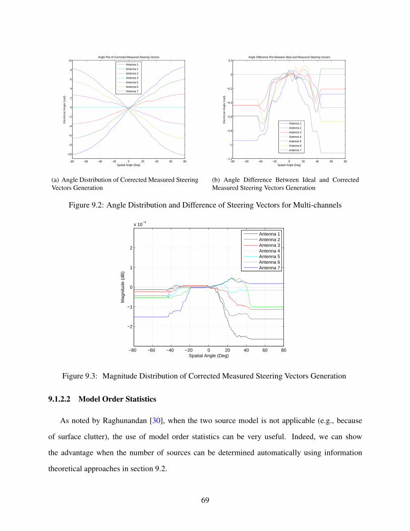
−80 −60 −40 −20 0 20 40 60 80
−10
−8
−6
−4
−2
0
2
4
6
8
10
Spatial Angle (Deg)
Ele
ctrica
l An
gle
(ra
d)
Angle Plot of Corrected Measured Steering Vectors
Antenna 1
Antenna 2
Antenna 3
Antenna 4
Antenna 5
Antenna 6
Antenna 7
(a) Angle Distribution of Corrected Measured SteeringVectors Generation
−80 −60 −40 −20 0 20 40 60 80−1.2
−1
−0.8
−0.6
−0.4
−0.2
0
0.2
Spatial Angle (Deg)
Ele
ctrica
l An
gle
(ra
d)
Angle Difference Plot Between Ideal and Measured Steering Vectors
Antenna 1
Antenna 2
Antenna 3
Antenna 4
Antenna 5
Antenna 6
Antenna 7
(b) Angle Difference Between Ideal and CorrectedMeasured Steering Vectors Generation
Figure 9.2: Angle Distribution and Difference of Steering Vectors for Multi-channels
−80 −60 −40 −20 0 20 40 60 80
−2
−1
0
1
2
x 10−4
Mag
nitu
de (
dB)
Spatial Angle (Deg)
Antenna 1Antenna 2Antenna 3Antenna 4Antenna 5Antenna 6Antenna 7
Figure 9.3: Magnitude Distribution of Corrected Measured Steering Vectors Generation
9.1.2.2 Model Order Statistics
As noted by Raghunandan [30], when the two source model is not applicable (e.g., because
of surface clutter), the use of model order statistics can be very useful. Indeed, we can show
the advantage when the number of sources can be determined automatically using information
theoretical approaches in section 9.2.
69

The observed or measured data can be modelled as the superposition of a finite number of
signals with additive noise. An accurate estimate of the number of sources is essential in many
signal processing problems such as in the DoA estimation by a smart antenna system, in the poles
retrieval of a system response, and in image processing. Early on, Bartlett proposed a hypothesis
testing procedure to test the signals by likelihood ratio statistics with pre-determined thresholds.
But the actual distribution of the test statistics can only be approximated and a choice of the level
of significance is required [38]. Approaches based on information criterion are becoming more
popular because of their accurate estimation performance. Two commonly used model selection
criteria are: Akaike Information Criterion (AIC), and Bayesian Information Criterion (BIC), which
is also named as Minimum Description Length Criterion. The number of signals for both criteria is
determined by simply minimizing the value of an information criterion. Many variations of these
two criteria have been proposed. However, they are existing benchmarks commonly used in model
selection problems in time series and regression analysis.
Given the observed data and a set of candidate probability models that depend on the parameter
vector Θ (including the eigenvalues and eigenvectors of the sample correlation matrix and noise
power), a model selection criterion selects the model order by minimizing a loss function and can
be expressed in the following form [38]:
A model selection criteria =−2logL(X |Θ)+P(L,kp) (9.1)
where L(X |Θ) is the likelihood function, Θ denotes the maximum likelihood estimate of Θ, L is the
sample size and kp is the number of freely-adjusted parameters (degrees of freedom) in Θ, which is
a function of both p and q. p is the number of nonzero eigenvalues and q is the number of sources.
The first term is a measure of the goodness of fit of the candidate model to the data. The second
term serves as a penalty term for over fitting.
AIC can be obtained when the penalty term in (9.1) is set to be 2kp [36],
AIC =−2logL(X |Θ)+2kp (9.2)
70

while for BIC, the penalty term is kp logL,
BIC =−2logL(X |Θ)+ kp logL (9.3)
where kp = q(2p− q)+ 1. The estimation performance can be effected by the actual number of
signals, signal strength, signal separations, signal correlations, number of snapshots, etc. In our
application, the 11 closely spaced along-track snapshots may correlate with each other, and 11
is a modest sample support. Thus we tend to choose BIC as our model order selection criterion
since BIC is consistent, showing great performance when incoming signals are correlated and
conquering the overestimation problem with AIC.
Note that, the expected number of signals in the data is two for ice bottom tomography with-
out surface clutter. With ice surface clutter, we would expect 4 signals to handle left and right
clutter. We assumed that there were no other sources of energy, although there is some possi-
bility that RFI or englacial targets may be present at times. Hence, we constrain the number of
sources estimated to be 2,3 or 4. To test the efficacy, we used the fixed two sources model and
automatically-determined number of sources model to initiate the DoA estimation procedure. Per-
formance comparison plots can be seen in section 9.2.
9.1.2.3 Bottom Smoothing
As illustrated in section 8.2, our dataset is actually a point cloud (MLE) consisting of thousands
of slices in the along-track dimension, and targets are resolved to each slice through SAR process-
ing. To simplify the problem, we fix the number of sources to two again in accordance with our
system model plot: one on the left and the other on the right. Our final goal is to improve height
estimation and obtain an artifact free 3D tomography image, in order to create a more accurate
DEM.
For either approach (MUSIC or MLE), each voxel in our matrix is assigned a scattering value
during signal processing. Generally, if there is no scattering target (i.e., ice bottom) in the voxel,
71

then the scattering value is small because only system noise contributed and we can discard these
points by a simple threshold method. In this way, most of the points are removed. However, in
some cases, because the noise is random and has a non-zero probability of being large at times and
we are often trying to see weak scatter targets, the threshold method is not sufficient. Here, we
would like to use a priori knowledge that we are imaging a slowly changing surface and mask bad
points out using this additional spatial knowledge as well.
The output data from the array processing routine is subjected to some post-processing steps.
Originally, the surface extraction routine for MLE is conducted as below. We first do an inter-
polation of layer data defined by hand-picked surface and bottom values that used the traditional
2D imagery. Through the surface and bottom information, we calculate an approximate range for
where the ice bottom would lie, which is the “mask”. The width of the mask is programmable.
Then we search for the maximum value in each cross-track frequency bin and keep track of which
range bin the maximum falls in. Using the tomography toolbox by Paden et al. [31], we find a
polynomial based function which converts time-delay to target (x coordinate), and direction of ar-
rival to a cross-track (y coordinate) and elevation position (z coordinate). In the end, we convert
geocentric data values to a geodetic coordinates, which means transform the (x,y,z) data into a
tuple of latitude, longitude and elevation. The 3D imaging of DEM is possible. We show the 2D
cross-track image for the original surface extraction routine of MLE in Fig. 9.4. The points in the
plot indicating the estimated ice bottom, which do not form a continuous line.
In our thesis, the modified surface extracting routine we have implemented seems to work
well and involves outlier filtering, maximization, interpolation and smoothing. These steps are
incorporated after the third step of original surface tracking routine (i.e. the maximum finding).
We use frame 20130410 01 033 from the 2013 Greenland P3 campaign to illustrate the denoising
procedure. The output figures display the distribution of the directions of arrival in terms of the
estimated relative signal power by these two algorithms. Note that, the MUSIC cepstrum does not
technically represent signal power, but is generally correlated to it.
Fig. 9.5(a) is an example of a single slice from the point cloud. We can see a lot of points
72

−80 −60 −40 −20 0 20 40 60 80
800
850
900
950
1000
1050
1100
1150
1200
1250
1300
Spatial Angles (Deg)
Ran
ge B
ins
DoA Estimation Using Base MLE Focusing on Bottom Region
Figure 9.4: DoA Distribution Using MLE Focusing on Bottom Region.
indicating the internal ice layers and ice bottom echoes and clutter (the ice surface is not visible
since it was received while the receiver blanking switch was on). It is easy to distinguish out the
ice bottom by eye, which is the region starting from range bin 850 and ending with about 1000
(a continuous line). However, if we zoom in to this bottom region, many discontinuities can be
seen as shown in Fig. 9.5(b). First, a quick observation about the shape of the basal scattering in
Fig. 9.5. For a flat surface and not taking into account the ice medium, the range versus incidence
angle θ is:
range =z0√
1− sin2(θ)(9.4)
where z0 is the height of the plane above the surface. This shape resembles a parabolic shape
which goes to infinity as θ goes to +/− 90 deg. In other words, if we transform to rectangular
coordinates, the basal scatterers in Fig. 9.5 would be a horizontal line if the surface was perfectly
flat. Now, if the intersection of the slice with the ice bottom always gave a positive return and the
ice bottom was continuous, we would expect a continuous line of scatterers which looks somewhat
parabolic with deviations caused by the ice bottom topography.
Since the surface does not produce a continuous line because of errors in the angle of arrival
73

estimates, we try to apply interpolation to fill up those discontinuities. First, we need to make
sure every frequency bin only has one good position value. If there is more than one position
value in a frequency bin, we take the mean of them. If there are no good position values for a
bin, we denote it as NaN. After the simple filling up procedure, we apply the outlier detection to
avoid bad samples distorting the data before interpolation. As assumed earlier, the ice bottom is
slowly changing. Thus large jumps between range bin values of adjacent frequency bins would
be considered as outliers. Here, we set the threshold to be 50, which means if any two adjacent
positions have a difference over 50, then it will be regarded as bad data and replaced with NaN. At
this point, we will fill in the gaps with linear interpolation between good values as follows:
value(index) = prevvalue +(nextvalue−prevvalue)× (index−previndex)
(nextindex−previndex)(9.5)
where index is the current direction of arrival angle index, value is the range bin position belonging
to the corresponding angle. prevvalue and nextvalue indicate the previous and next existing range
bin position for the current angle index, respectively. Similarly, previndex and nextindex represent
the previous and next angle index where there exists range bin good position values. A scatter
plot regarding range bin position for each angle index is shown in figure 9.5(c). In the end, the
“Savitzky-Golay” method [39] is applied to smooth the result because of its ability to smooth the
data without greatly distorting the signal. Its principle is to fit successive sub-sets of adjacent
data points with a low-degree polynomial by the method of linear least squares. The resulting
smoothing performance is shown in figure 9.5(d) as the red line, while comparing to the blue
asterisks representing the un-smoothed bottom.
In section 8.4.1, we noted that MUSIC and MLE are different when you break them into their
respective eigenstructures. Also, MLE just produces two discrete angle estimates (one from the
left and one from the right) as opposed to MUSIC, where the cepstrum that is used has a value for
every direction of arrival and sources are distinguished by large values. Hence, MUSIC produces a
smooth angular distribution compared to MLE. This is because when MLE gets the wrong scatter
74

(a) DoA Distribution for the Whole Elevation Dimen-sion
−80 −60 −40 −20 0 20 40 60 80
0
50
100
150
200
250
300
350
400
450
500
Spatial Angles (Deg)
Ra
ng
e B
ins
DoA Estimation Using MLE Focusing on Bottom Region
(b) DoA Distribution Zoom in Bottom Region WithGuard Lines
−80 −60 −40 −20 0 20 40 60 80
0
50
100
150
200
250
300
350
400
450
500
Spatial Angles (Deg)
Ra
ng
e B
ins
Scatter Plot of Bottom Region After Interpolation
(c) DoA Distribution After Interpolation
−80 −60 −40 −20 0 20 40 60 80
0
50
100
150
200
250
300
350
400
450
500
Spatial Angles (Deg)
Ra
ng
e B
ins
Scatter Plot of Bottom Region After Smoothing
InterpolationSmooth
(d) DoA Distribution After Interpolation and Smooth-ing
Figure 9.5: DoA Estimation Using MLE for First Record of Frame 20130410 01 033
location (e.g. because the ice bottom SNR has dropped too low), we might get a point target with
a large angular error whereas the MUSIC cepstrum will tend to still have some peak near where
the ice bottom actually is (although it might not be one of the two dominant peaks). This can
be seen in the comparison between Fig. 9.5(b) (MLE) and Fig. 9.6 (MUSIC), the expected mask
(“the range between two red lines”) is trying to restrict the tracing region of ice bottom. We regard
peaks outside this region as bad data. As highlighted in Fig. 9.6 for MUSIC, there may be peaks
outside the mask, but the neighbourhood region still contains a peak. But for MLE in Fig. 9.5(b),
75

if a peak is outside the mask region, we totally lose the information related to this estimate. That is
the reason why the base surface tracking routine of MUSIC performs better than the base routine
of MLE.
Figure 9.6: DoA Distribution Using MUSIC Focusing on Bottom Region.
9.1.2.4 Speed Up MLE-AP
The processing time is an important metric we should take into account. Though we utilize the
computationally attractive alternating projection method to compute the multi-dimensional ML
estimator, it is still much slower than the MUSIC algorithm. As discussed in [30] and our data
processing procedure, MUSIC takes 0.5s to process one range line while MLE needs 22.64s. Nor-
mally, the point cloud contains thousands of range lines, which means MLE is thousands of times
slower than the MUSIC algorithm. Indeed, this is the case, for one data frame, MUSIC only needs
2 minutes while MLE takes almost six hours. We still need to speed it up without decreasing the
spatial resolution.
If we set the spatial resolution to 1 degree (that is 181 equally spaced spatial-frequency bins),
we need 181 operations to get the maximum. However, note that, for an airborne-radar with only
seven antenna elements, we don’t need this level of accuracy to find the approximate location of
76

the global maximum, especially for the initialization step in the MLE-AP algorithm. Hence, we
can do a sparse grid search followed by function optimization. For example, we first loosen the
angle steps from −90 : 1 : 90 to −90 : 5 : 90 and conduct the initialization step. After determining
which range bin the maximum falls into, say 36, we tighten the angle range again around 36,
which is 30,31, · · · ,36,37, · · · ,40. In this manner, we maintain the resolution to be 1 degree, but
the number of operations effectively reduced from 181 to 48, almost four times less work load.
Actually, the loose grid size can be programmable. Through implementation, the running time for
one range line decreases in half, from 22.64s to 11.55s. And the total running time for one data
segment reduce from 6 hours to around 1 hour. Moreover, the performance of 3D tomographic
cross-over analysis is as good as before.
9.2 Output From Greenland Dataset
The data frames used for the comparison of the algorithms are 20130404 02 040 and 20130410 01 033.
These crossing flight lines were collected near Jakobshavn Glacier in southwestern Greenland. The
flight pattern and echograms are illustrated in Fig. 9.7. Fig. 9.7(a) and Fig. 9.7(b) are the flight
paths for the two data segments, while Fig. 9.7(c) and Fig. 9.7(d) draw the flight pattern of these
two days together with the highlighted lines corresponding to the specific data frames of interest.
The radar echograms for these two data frames are shown in Fig. 9.7(e) and Fig. 9.7(f) respectively.
These radar echograms are made by forming a fixed beam at nadir with the array where the vertical
dimension is elevation and the horizontal dimension is along the aircraft’s flight trajectory.
These two data frames were chosen because they cross each other in a region where the ice
bottom is rough enough to backscatter sufficient energy to the radar that can be used to form a
DEM. Although we do not know the actual ice bottom elevation, we know that the algorithms
should be self consistent. Since it is impractical to determine the actual elevation, we compare the
algorithm produced DEMs from the two crossing lines and assume that a lower mean squared error
between the DEMs means that the algorithm is performing better (i.e. it is more self consistent).
77

(a) Flight Path for Segment20130404 02 040
(b) Flight Path for Segment20130410 01 033
(c) Flight Pattern for Cross-over Analysis of DataFrame 20130404 02 040
(d) Flight Pattern for Cross-over Analysis of DataFrame 20130410 01 033
(e) Echogram of Data Frame 20130404 02 040 (f) Echogram of Data Frame 20130410 01 033
Figure 9.7: Flight Pattern and Echograms
78
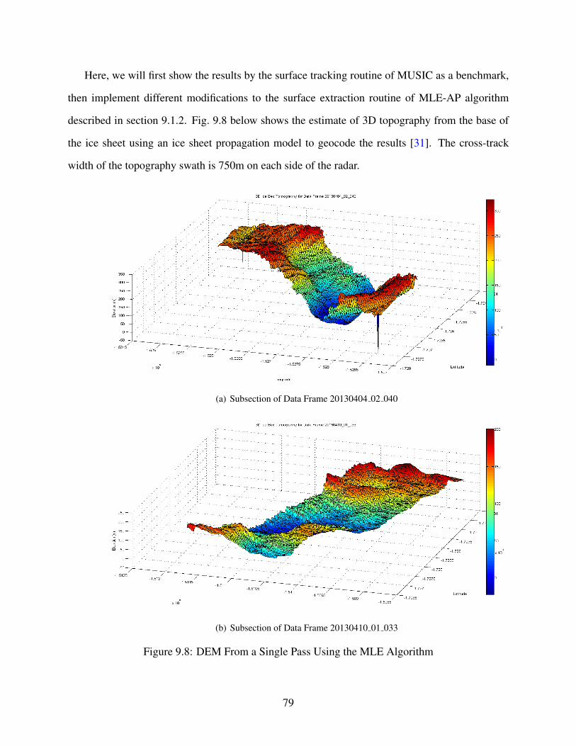
Here, we will first show the results by the surface tracking routine of MUSIC as a benchmark,
then implement different modifications to the surface extraction routine of MLE-AP algorithm
described in section 9.1.2. Fig. 9.8 below shows the estimate of 3D topography from the base of
the ice sheet using an ice sheet propagation model to geocode the results [31]. The cross-track
width of the topography swath is 750m on each side of the radar.
(a) Subsection of Data Frame 20130404 02 040
(b) Subsection of Data Frame 20130410 01 033
Figure 9.8: DEM From a Single Pass Using the MLE Algorithm
79

In Fig. 9.9, the cross-over region of these two frames is presented. We can see clearly that
there exists a valley in the middle of the plot, just as indicated by the little hollow in Fig. 9.7(e)
and Fig. 9.7(f) where the dashed lines lie. The two plots match very well, and we can confirm
that this is indeed the overlapping region. The difference statistics between the two DEMs, mean
(MEAN), standard deviation (STD) and root mean squared error (RMSE), are shown in Table 9.1
for comparison.
MUSIC algorithm for for cross−over region of data segment 20130404_02_040
660 680 700 720 740 760
470
480
490
500
510
520
530
540
550
560
570
250
300
350
400
(a) Data Frame 20130404 02 040
MUSIC algorithm for for cross−over region of data segment 20130410_01_033
660 680 700 720 740 760
470
480
490
500
510
520
530
540
550
560
570
250
300
350
400
(b) Data Frame 20130410 01 033
Figure 9.9: Cross-Over Analysis by MUSIC
As for MLE-AP, if we directly apply the algorithm without bottom smoothing, the results are
poor as shown in Fig. 9.10. It is very hard to tell that these two plots are for the same overlapping
region, because they don’t really look the same. Throughout the whole experimental process, we
found that bottom smoothing is the crucial step to improve the performance of the surface tracking
routine of MLE-AP algorithm. Without it, the plots will be messy because MLE always produces
some artifacts. After our denoising routine, we can see the results in Fig. 9.11, which match very
well with the benchmark produced by the MUSIC algorithm. The valley clearly shows up again.
The next step is to replace ideal steering vectors with the measured steering vectors look-up
table. The results are shown in Fig. 9.12. The cross-over plots using model order statistics are given
in Fig. 9.13. We can see no big difference between Fig. 9.11, Fig. 9.12 and Fig. 9.13. Moreover,
from the statistics comparison in Table 9.1, we can see that the results produced by measured
80
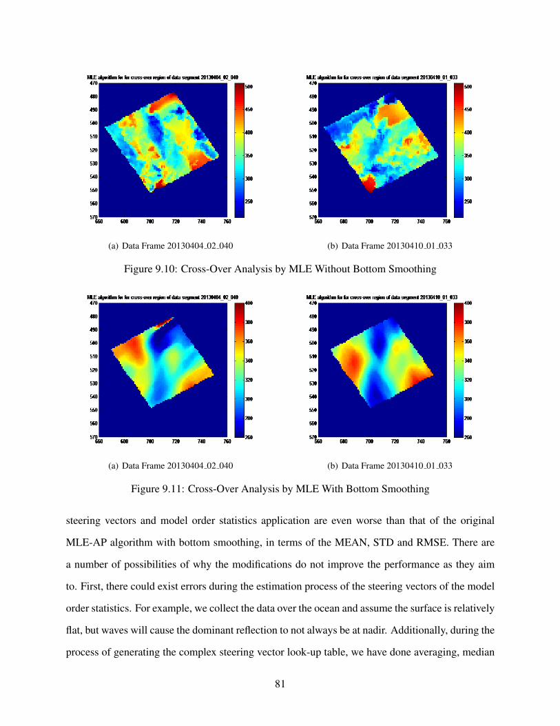
(a) Data Frame 20130404 02 040 (b) Data Frame 20130410 01 033
Figure 9.10: Cross-Over Analysis by MLE Without Bottom Smoothing
(a) Data Frame 20130404 02 040 (b) Data Frame 20130410 01 033
Figure 9.11: Cross-Over Analysis by MLE With Bottom Smoothing
steering vectors and model order statistics application are even worse than that of the original
MLE-AP algorithm with bottom smoothing, in terms of the MEAN, STD and RMSE. There are
a number of possibilities of why the modifications do not improve the performance as they aim
to. First, there could exist errors during the estimation process of the steering vectors of the model
order statistics. For example, we collect the data over the ocean and assume the surface is relatively
flat, but waves will cause the dominant reflection to not always be at nadir. Additionally, during the
process of generating the complex steering vector look-up table, we have done averaging, median
81

filtering, interpolation and smoothing. Each routine will probably reduces noise, but also lowers
the resolution of the steering vector estimation. Finally, we only test one dataset and it is not a
sufficiently large sample to say that either of these routines failed or succeeded in improving the
MSE in general.
(a) Data Frame 20130404 02 040 (b) Data Frame 20130410 01 033
Figure 9.12: Cross-Over Analysis by MLE With Measured Steering Vectors
(a) Data Frame 20130404 02 040 (b) Data Frame 20130410 01 033
Figure 9.13: Cross-Over Analysis by MLE With Model Order Statistics
The final step is to incorporate quality metrics into the culling process, i.e., backscattered signal
strength and the likelihood value of the objective function. A bigger value of backscattered signal
82

spectrum indicates a greater possibility that there exists a target. Similarly, the larger the likelihood
value, the more confident we are that the target lies in that angle bin. This is an effective procedure
to mask out the artifacts made by MLE.
To do this, we remove bad points if they fall below a threshold backscattered signal strength
and/or the likelihood objective function value. We first show the backscattered signal power dis-
tribution of the overlapping region in Fig. 9.14(a) and 9.14(b). Since the values cover a wide
dynamic range, log-scaled plots are presented. We set the bad point threshold to be −75, which
means any backscattered power value less than −75 will be considered an artifact and be masked
out from the cross-over plots. We chose −75 as the threshold because it gave the best cross-over
performance. The results can be seen in Fig. 9.14(c) and Fig. 9.14(d). The difference results are
only slightly improved and are given in Table 9.1. We also test the likelihood value metric, but
the difference result is similar. This makes sense, since the distribution of the likelihood value in
Fig. 9.15(a) and Fig. 9.15(b) is very similar to the backscattered signal power shown in Fig. 9.14(a)
and Fig. 9.14(b).
Table 9.1: Difference Statistics Comparison between MUSIC and Various Applications of MLE-AP Algorithm
Algorithm MEAN STD RMSE MAX DIFF MIN DIFFMUSIC 20.33 21.93 29.90 143.50 0.0017
MLE-AP 62.86 47.62 78.86 286.92 0.0146MLE-AP WITH SMOOTHING 17.62 14.98 23.13 162.79 0.0056MLE-AP WITH MEASURED 20.23 14.87 25.43 158.31 0.0094
MLE-AP WITH MODEL ORDER 19.64 14.79 24.58 76.13 0.0078MLE-AP WITH QUALITY METRIC 18.52 14.06 23.25 76.13 0.0078
From the statistics of Table 9.1 (MAX DIFF and MIN DIFF indicate the maximum and mini-
mum difference value between two single pass images, respectively), we can see that after bottom
smoothing, the surface extraction routine of MLE-AP indeed performs better than the surface ex-
traction routine of MUSIC. All three criteria are lower. This supports the conclusion that these
variations of the surface extraction routine of MLE are effective post-processing routines for imag-
ing of 3D ice bed tomography. Since model order statistics, measured steering vectors, and quality
83
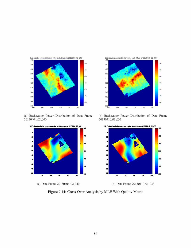
Back scatter power distribution in log scale (MLE) for 20130404_02_040
660 680 700 720 740 760
470
480
490
500
510
520
530
540
550
560
570
−80
−75
−70
−65
−60
−55
−50
(a) Backscatter Power Distribution of Data Frame20130404 02 040
Back scatter power distribution in log scale (MLE) for 20130410_01_033
660 680 700 720 740 760
470
480
490
500
510
520
530
540
550
560
570
−80
−75
−70
−65
−60
−55
−50
(b) Backscatter Power Distribution of Data Frame20130410 01 033
(c) Data Frame 20130404 02 040 (d) Data Frame 20130410 01 033
Figure 9.14: Cross-Over Analysis by MLE With Quality Metric
84
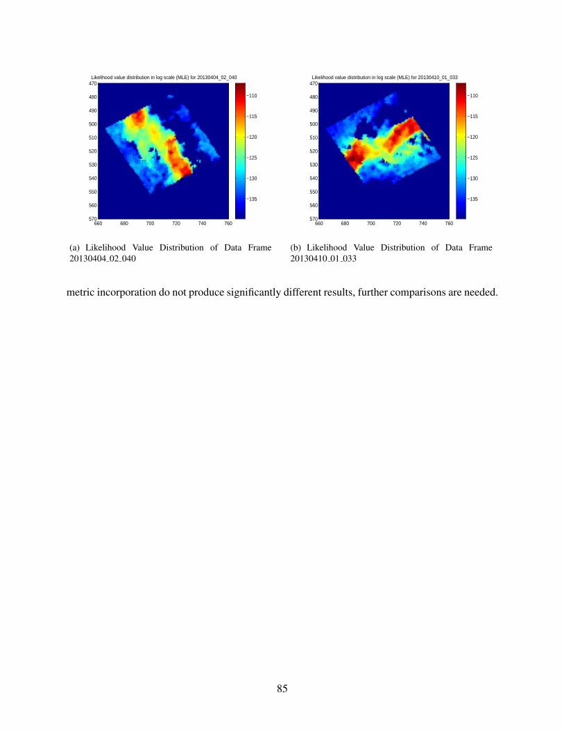
Likelihood value distribution in log scale (MLE) for 20130404_02_040
660 680 700 720 740 760
470
480
490
500
510
520
530
540
550
560
570
−135
−130
−125
−120
−115
−110
(a) Likelihood Value Distribution of Data Frame20130404 02 040
Likelihood value distribution in log scale (MLE) for 20130410_01_033
660 680 700 720 740 760
470
480
490
500
510
520
530
540
550
560
570
−135
−130
−125
−120
−115
−110
(b) Likelihood Value Distribution of Data Frame20130410 01 033
metric incorporation do not produce significantly different results, further comparisons are needed.
85

Chapter 10
Conclusion and Future Work
This paper illustrates the application of DoA estimation techniques to SAR processed datasets.
The fundamental approach in each of the algorithms underline a different concept with specific
assumptions encompassing the system model. While the MLE algorithm resorts to a classical
statistical inference model based on the likelihood function, MUSIC uses the sample correlation
matrix to derive eigenspace matrices.
Although MLE has better projected performance compared to MUSIC in the low SNR regime,
it is computationally the most expensive. For the antenna array geometry and sample support used
in ice bed SAR tomography for this report, the surface extraction routine of MUSIC performs better
than the base surface extraction routine of MLE-AP algorithm even though it does not exhibit the
same probability of source separability for sources located close to each other.
We applied several techniques to improve the base surface extraction routine of the MLE ap-
proach. These are to replace ideal steering vector generation with measured steering vectors, au-
tomatic determination of the number of scatter sources, smoothing to remove outliers and reduce
noise, and quality metrics to remove bad estimates. After the application of all these techniques, the
surface extraction routine of MLE outperforms the surface extraction routine of MUSIC in terms
of cross-over analysis. It supports the conclusion that MLE is indeed the optimal estimator for
our particular ice bed tomographic application. Note that the spatial bottom smoothing aiming to
86

remove the artifacts made by the MLE algorithm, is the most essential step in the post-processing
procedure.
For now, we are just using simple interpretation, maximization and smoothing techniques. To
improve the results, we suggest the following for future work. There exists advanced surface and
volume finding routines for noisy point clouds in the field of image processing and the application
of these routines would very likely improve the results substantially. The surface tracking routines
should incorporate the a priori knowledge that the ice bottom is generally smooth and single valued
(i.e. no folding or overhangs). Currently, the surface extraction forces a single range value per
direction of arrival which works well at nadir, but towards the edges of the swath it would be better
to search for the best direction of arrival per range. Currently the data processing uses f-k migration
for SAR processing and only a single aperture is used. Snapshots are gathered from a neighborhood
of pixels. Also, we have used the narrowband approximation for the system model which is not
quite valid for most of the datasets. Improved results may be obtained by the application of sub-
band and sub-aperture processing to enable spatial smoothing of SAR processed datasets, coupled
with enhanced clutter rejection techniques. Also, f-k migration is a Fourier based technique for
applying the matched filter. While it is faster, it is not as accurate as time domain back projection
which applies convolution directly because the matched filter is actually a space-time varying filter
due to non-linear flight paths and sloped ice surfaces.
In conclusion, this work extends our understanding of the MLE algorithm’s application to ice
bottom tomography. A speed improvement to the MLE algorithm was made. We also tested the
application of several post-processing routines to get the best surface out of the MLE algorithm.
In this process, we developed a method for extracting measured steering vector coefficients from
calibration data taken over the ocean, although the application of these coefficients did not show
much change in the results. Finally, we have suggested a number of methods that might improve
the results further.
87
References
[1] Brahima Sanou. The world in 2013: ICT Facts and Figures. International Telecommunica-
tions Union (ITU), February 2013.
[2] Cisco Systems. Cisco Visual Networking Index: Global Mobile Data Traffic Forecast Update,
2012-2017. Cisco, February 2013.
[3] Arogyaswami J. Paulraj, Dhananjay A. Gore, Rohit U. Nabar, and Helmut Bolcskei. An
overview of MIMO communications - a key to gigabit wireless. in Proceedings of the IEEE,
92:198–218, February 2004.
[4] Thomas L. Marzetta. Noncooperative Cellular Wireless with Unlimited Numbers of Base Sta-
tion Antennas. IEEE Transactions on Wireless Communications, 9(11):3590 – 3600, Novem-
ber 2010.
[5] Hoon Huh, Giuseppe Caire, Haralabos C. Papadopoulos, and Sean A. Ramprashad. Achiev-
ing ”Massive MIMO” spectral efficiency with a not-so-large number of antennas. IEEE
Transactions on Wireless Communications, 11:3226 – 3239, September 2012.
[6] Younsun Kim, Hyoungju Ji, Hyojin Lee, Juho Lee, Boon Loong Ng, and Jianzhong(Charlie)
Zhang. Evolution Beyond LTE-Advanced with Full Dimension MIMO. IEEE International
Conference on Communications 2013: IEEE ICC’13 - Workshop Beyond LTE-A, pages 111–
115, June 2013.
[7] Akbar M. Sayeed and Thiagarajan Sivanadyan. Wireless Communication and Sensing in
88
Multipath Environments Using Multi-antenna Transceivers. Chapter for Handbook on Array
Processing and Sensor Networks, K. J. R. Liu and S. Haykin, Eds. Wiley, 2010.
[8] M. Larsen, A. Swindlehurst, and T. Svantesson. Performance Bounds for MIMO-OFDM
Channel Estimation. IEEE Transactions on Signal Processing, 57(5):1901–1916, May 2009.
[9] Yung-Yi Wang, Jiunn-Tsair Chen, and Wen-Hsien Fang. TST-MUSIC for joint DOA-delay
estimation. IEEE Transactions on Signal Processing, 49(4):721–729, April 2001.
[10] A.L.F. de Almeida. Tensor Modeling and Signal Processing for Wireless Communication
Systems. PhD. dissertation, University of Nice Sophia Antipolis (UNS), Sophia Antipolis,
France, November 2007.
[11] M. Haardt and Josefa A. Nossek. Simultaneous Schur decomposition of several nonsymmet-
ric matrices to achieve automatic pairing in multidimensional harmonic retrieval problems.
IEEE Transactions on Signal Processing, 46(1):161–169, January 1998.
[12] Anding Wang, Lingjia Liu, and Jianzhong Zhang. Low Complexity Direction of Arrival
(DoA) Esitmation for 2D Massive MIMO Systems. In IEEE GLOBECOM Workshop on
Emerging Technologies for LTE-Advanced and Beyond-4G, December 2012.
[13] Alle-Jan van der Veen, Michaela C. Vanderveen, and Arogyaswami Paulraj. Joint angle and
delay estimation using shift-invariance techniques. IEEE Transactions on Signal Processing,
46(2):405–418, February 1998.
[14] R. Roy and T. Kailath. ESPRIT-estimation of signal parameters via rotational invariance
techniques. IEEE Transactions on Acoustics, Speech and Signal Processing, 37(7):984–995,
July 1989.
[15] M.D. Zoltowski, M. Haardt, and C.P. Mathews. Closed-form 2-D angle estimation with
rectangular arrays in element space or beamspace via Unitary ESPRIT. IEEE Transactions
on Signal Processing, 44:316–328, February 1996.
89

[16] M. Haardt, F. Roemer, and G. Del Galdo. Higher-order SVD based subspace estimation to im-
prove the parameter estimation accuracy in multi-dimensional harmonic retrieval problems.
IEEE Transactions on Signal Processing, 56:3198–3213, July 2008.
[17] J.F. Cardoso and A. Souloumiac. Blind beamforming for non-Gaussian signals. Radar and
Signal Processing, IEE Proceedings F, 140(6):362 – 370, December 1993.
[18] J.F. Cardoso and A. Souloumiac. Jacobi Angles For Simultaneous Diagonalization. SIAM
Journal on Matrix Analysis and Applications, 17(1):161 – 164, January 1996.
[19] Lieven De Lathauwer, Bart De Moor, and Joos Vandewalle. Jacobi Angles For Simultaneous
Diagonalization. SIAM Journal on Matrix Analysis and Applications, 21(4):1253 – 1278,
May 1996.
[20] Yi Zhu, Lingjia Liu, Anding Wang, Krishna Sayana, and Jianzhong Zhang. DoA Estimation
and Capacity Analysis for 2D Active Massive MIMO Systems. Proceedings of the IEEE
International Conference on Communications, pages 4630 – 4634, June 2013.
[21] Jakob Hoydis, Stephan ten Brink, and Merouane Debbah. Massive MIMO: How many an-
tennas do we need? arXiv:1107.1709v2 [cs.IT], Septermber 2011.
[22] Fredrik Rusek, Daniel Persson, Buon Kiong Lau, Erik G. Larsson, Thomas L. Marzetta, Ove
Edfors, and Fredrik Tufvesson. Scaling up MIMO: Opportunities and Challenges with Very
Large Arrays. arXiv:1201.3210v1 [cs.IT], January 2012.
[23] Ansuman Adhikary, Junyoung Nam, Jae-Young Ahn, and Giuseppe Caire. Joint Spatial Di-
vision and Multiplexing. arXiv:1209.1402 [cs.IT], January 2013.
[24] A. Lee Swindlehurst and Thomas Kailath. A Performance Analysis of Subspace-Based Meth-
ods in the Presence of Model Errors: Part II - Multidimensional Algorithms. IEEE Transac-
tions on Signal Processing, 41(9):2882–2890, September 1993.
90

[25] T.L. Marzetta. How Much Training is Required for Multiuser Mimo? Signals, Systems and
Computers, 2006. ACSSC ’06. Fortieth Asilomar Conference on, pages 359 – 363, October
2006.
[26] Song Noh, Michael D. Zoltowski, Youngchul Sung, and David J. Love. Pilot Beam Pat-
tern Design for Channel Estimation in Massive MIMO Systems. arXiv:1309.7430v2 [cs.IT],
January 2014.
[27] Florian Roemer and Martin Haardt. A framework for the analytical performance
assessment of matrix and tensor-based ESPRIT-type algorithms. September 2012.
http://arxiv.org/abs/1209.3253.
[28] National Oceanic and Atmospheric Administration (NOAA) National Ocean Service. Is Sea
Level Rising. June 2014.
[29] John Paden. Synthetic aperture radar for imaging the basal conditions of the polar ice sheets.
University of Kansas, PhD Dissertation, August 2006.
[30] Sahana Raghunandan. Analysis of Angle of Arrival Estimation Algorithms for Basal Ice Sheet
Tomography. CReSIS Techical Reports p. 57., August 2013.
[31] John Paden, Torry Akins, David Dunson, Chris Allen, and Prasad Gogineni. Ice-sheet bed
3-D tomography. Journal of Glaciology, 56(195):3 – 11, April 2010.
[32] J. Paden, C. Allen, and P. Gogineni. 3D imaging of ice sheets. Geoscience and Remote
Sensing Symposium (IGARSS), 2010 IEEE International, pages 2611–2613, July 2010.
[33] R.O Schmidt. Multiple Emitter Location and Signal Parameter Estimation. IEEE Trans.
Antennas Propagation, AP-34(3):276–280, March 1986.
[34] V. F. Pisarenko. The Retrieval of Harmonics from a Covariance Function. Geophysical
Journal of the Royal Astronomical Society, 33(3):347 – 366, September 1973.
91
[35] Simon O. Haykin. Adaptive Filter Theory, 5th Edition. Prentice Hall, ISBN-13:
9780132671453, 2013.
[36] Harry L. Van Trees. Optimum Array Processing (Detection, Estimation, and Modulation
Theory, Part IV). Wiley-Interscience, 2002.
[37] I. Ziskind and M. Wax. Maximum likelihood localization of multiple sources by alternating
projection. Acoustics, Speech and Signal Processing, IEEE Transactions on, 36(10):1553 –
1560, October 1988.
[38] P. Chen, T.-J. Wu, and J. Yang. A comparative study of model selection criteria for the
number of signals. Radar, Sonar and Navigation, IET, 2(3):180 – 188, June 2008.
[39] Abraham. Savitzky and M. J. E. Golay. Smoothing and Differentiation of Data by Simplified
Least Squares Procedures. Analytical Chemistry, 36(8):1627 – 1639, July 1964.
92