matr ix mathstrack here the matrix - university of … · 2.4 calculating the inverse of an n ! n...

MathsTrack

MATHEMATICS LEARNING SERVICE

Centre for Learning and Professional Development

Level 1, Schulz Building (G3 on campus map)

TEL 8303 5862 | FAX 8303 3553 | [email protected]

www.adelaide.edu.au/clpd/maths/

Module 9

Introduction to Matrices

Income = Tickets ! Price

=

�

250 100

350 150

!

" #

$

% &

25 30 35

20 15 10

!

" #

$

% &

=

�

8,250 9,000 9,750

11,750 12,750 13,750

!

" #

$

% &

(NOTE Feb 2013: This is the old version of MathsTrack.New books will be created during 2013 and 2014)

Topic 2

Matrices

(A+B) + C = A+ (B + C) h(kA) = (hk)A (AB)C = A(BC)

2.1. SYSTEMS OF LINEAR EQUATIONS 27

Examplesystem of

non-linearequations

The pair of equations4x2

1 + 2x2 = 42!

x1 " 3x2 = 2

is also called a system of equations, but in this case the equations are non-linear: each variable in a linear equation must occur to the first power only.

A system of linear equations can be expressed as a single matrix equation AX = B,which may be solved using matrix ideas.

Examplea matrixequation

The system of equations

3x1 + 4x2 + x3 = 12x1 + 3x2 = 44x1 + 3x2 " x3 = "2

can be written as the matrix equation

!

"3 4 12 3 04 3 "1

#

$

!

"x1

x2

x3

#

$ =

!

"14"2

#

$ ,

that is, in the form AX = B, where

A =

!

"3 4 12 3 04 3 "1

#

$ , X =

!

"x1

x2

x3

#

$ and B =

!

"14"2

#

$ ,

. . . which can be solved for the unknown matrix X.

A general system of m equations in n unknowns

a11x1 + a12x2 + · · · + a1nxn = b1

a21x1 + a22x2 + · · · + a2nxn = b2...

......

...am1x1 + am2x2 + · · · + amnxn = bm

can always be represented as a matrix equation of the form

AX = B

where

A =

!

%%%"

a11 a12 . . . a1n

a21 a22 . . . a2n...

......

am1 am2 . . . amn

#

&&&$, X =

!

%%%"

x1

x2...

xn

#

&&&$and B =

!

%%%"

b1

b2...bn

#

&&&$.

Here the matrix A is called the coe!cient matrix of the system of equations.

36 CHAPTER 2. INVERSES OF SQUARE MATRICES

2.4 Calculating the Inverse of an n! n Matrix

The most e!cient way of calculating the inverse of a square matrix is to use eleme-natry row operations.

This is best shown by example on a 3! 3 matrix: To find the inverse of

A =

!

"2 7 11 4 "11 3 0

#

$ ,

construct the augmented-matrix [A|I] from A and the identity matrix I of order 3:

[A|I] =

!

"2 7 1 1 0 01 4 "1 0 1 01 3 0 0 0 1

#

$ ,

then use elementary row operations to convert this into the form [I|B], having theidentity matrix of order 3 in the first three columns:

[I|B] =

!

"1 0 0 b11 b12 b13

0 1 0 b21 b22 b23

0 0 1 b31 b32 b33

#

$ .

If you can do this, then the matrix B is the inverse of A. If you can not, then Adoes not have an inverse.

There are three elementary row operations which can used for this procedure.

Elementary Row Operations(1) Interchange two rows.(2) Multiply or divide one row by a non-zero number.(3) Add a multiple of one row to another row.

To keep track of the our operations, we use the notation:

(1) Ri ! Rj to mean interchange row i and row j.(2) Ri # cRi to mean replace row i by row i multiplied by c.(3) Rj # Rj + cRi to mean to add row i multiplied by c to row j.

Examplecalculatingthe inverse

matrix

To change the augmented matrix

!

"2 7 1 1 0 01 4 "1 0 1 01 3 0 0 0 1

#

$

into the form [I|B]

• interchange row 1 and row 2, so that the (1, 1)-element becomes 1.


Examplematrixproduct Let A = det

!3 52 4

"and B = det

!1 23 4

", then det A = 2 and det B = !2.

As AB =

!3 52 4

" !1 23 4

"=

!18 2614 20

", we can see that det(AB) = !4.

This is an example of det(AB) = det A det B.

Examplematrixpowers

Let A be a 2" 2 matrix. Show that det(A2) = (det A)2.AnswerAs A2 = AA, det(A2) = det AA = det A det A = (det A)2.

Determinants can also be defined for square matrices of order n, and these have thesame properties as the determinants of square matrices of order 2. The formula fora determinant of order 3:

det A = a11a22a33 + a12a23a31 + a13a21a32 ! a13a22a31 ! a11a23a32 ! a12a21a33

You can avoid memorising this formula by using the pictures below:

(a)

!!

!!

!!"

##

##

##$

a11 a12

a21a22

(b)

!!

!!

!!

!!"

!!

!!

!!

!!"

!!

!!

!!

!!"

##

##

##

##$

##

##

##

##$

##

##

##

##$

a31 a32 a33

a21 a22 a23

a11 a12 a13

a31 a32

a21 a22

a11 a12

The formula for a 2 " 2 determinant is obtained from diagram (a) by multiplyingthe terms on each arrow together, then subtracting those on the arrows going fromleft to right from those on the arrow going from right to left. The formula for a 3"3determinant is obtained from diagram (b) similarly.

The formula for a general n" n determinant can be obatined by writing the matrixdown twice, with the copy along side the original as in (b), drawing n arrows goingfrom left to right and n arrows going from right to left as in (b), then continuing asin the 3" 3 case.

There is a general formula for the inverse of a square matrix of order n, but thecalculation takes a lot of time and a more e!cient method is shown in the nextsection.

Exercise 2.3

1. What is the inverse of the matrix

A =

!1 23 4

".


Examplematrixproduct Let A = det

!3 52 4

"and B = det

!1 23 4

", then det A = 2 and det B = !2.

As AB =

!3 52 4

" !1 23 4

"=

!18 2614 20

", we can see that det(AB) = !4.

This is an example of det(AB) = det A det B.

Examplematrixpowers

Let A be a 2" 2 matrix. Show that det(A2) = (det A)2.AnswerAs A2 = AA, det(A2) = det AA = det A det A = (det A)2.


det A = a11a22a33 + a12a23a31 + a13a21a32 ! a13a22a31 ! a11a23a32 ! a12a21a33

You can avoid memorising this formula by using the pictures below:

(a)

!!

!!

!!"

##

##

##$

a11 a12

a21a22

(b)

!!

!!

!!

!!"

!!

!!

!!

!!"

!!

!!

!!

!!"

##

##

##

##$

##

##

##

##$

##

##

##

##$

a31 a32 a33

a21 a22 a23

a11 a12 a13

a31 a32

a21 a22

a11 a12

The formula for a 2 " 2 determinant is obtained from diagram (a) by multiplyingthe terms on each arrow together, then subtracting those on the arrows going fromleft to right from those on the arrow going from right to left. The formula for a 3"3determinant is obtained from diagram (b) similarly.

The formula for a general n" n determinant can be obatined by writing the matrixdown twice, with the copy along side the original as in (b), drawing n arrows goingfrom left to right and n arrows going from right to left as in (b), then continuing asin the 3" 3 case.

There is a general formula for the inverse of a square matrix of order n, but thecalculation takes a lot of time and a more e!cient method is shown in the nextsection.

Exercise 2.3


A =

!1 23 4

".

A−1 =1

a11a22 − a12a21

[a22 −a12

−a21 a11

]

MATHS LEARNING CENTRELevel 3, Hub Central, North Terrace Campus, The University of AdelaideTEL 8313 5862 — FAX 8313 7034 — [email protected]/mathslearning/

This Topic . . .

Matrices1 were originally introduced as an aid to solving simultaneous linear equa-tions, but now have an important role in many areas of pure and applied mathe-matics. Today, matrix theory is used in business, economics, statistics, engineering,operations research, biology, chemistry, physics, meterology, etc. Matrices may con-tain many thousands of numbers, and need to be analysed with computers.

This topic introduces the theory of matrices. For convenience, the examples andexercises in the topic use small matrices, however the ideas are applicable to matricesof any size.

The topic has 2 chapters:

Chapter 1 introduces matrices and their entries. It begins by showing how ma-trices are related to tables, and gives examples of the different ways matricesand their entries can be described and written down.

Matrix algebra is introduced next. Equality, matrix addition/subtraction,scalar multiplication and matrix multiplication are defined. Examples showhow these ideas arise naturally from real life situations, and how matrix algebragrows out of practical applications. The rules for the algebra of matricesare based upon the rules of the algebra of numbers. Some of these rules areintroduced, and their connection with the corresponding rules for real numbersis described.

After reading this chapter, you will have a good idea of what matrices are,and will see how your previous knowledge carries across into matrices.

Chapter 2 introduces the inverse of a square matrix. The chapter shows how asystem of linear equations can be written as a matrix equation, and how thiscan be solved using the idea of the inverse of a matrix. Not all matriceshave inverses, so the questions of which matrices have inverses and how theseinverses are calculated are looked at.

Auhor: Dr Paul Andrew Printed: February 24, 2013

1matrices is the plural of matrix

i

Contents

1 The Algebra of Matrices 1

1.1 Matrices and their Entries . . . . . . . . . . . . . . . . . . . . . . . . 1

1.2 Equality, Addition and Multiplication by a Scalar . . . . . . . . . . . 4

1.3 Rules of Matrix Algebra (Part I) . . . . . . . . . . . . . . . . . . . . 10

1.4 Matrix Multiplication . . . . . . . . . . . . . . . . . . . . . . . . . . . 15

1.5 Rules of Matrix Algebra (Part II) . . . . . . . . . . . . . . . . . . . . 19

1.6 The Identity Matrices . . . . . . . . . . . . . . . . . . . . . . . . . . . 21

1.7 Powers of Square Matrices . . . . . . . . . . . . . . . . . . . . . . . . 22

1.8 The Transpose of a Matrix . . . . . . . . . . . . . . . . . . . . . . . . 24

2 Inverses of Square Matrices 26

2.1 Systems of Linear Equations . . . . . . . . . . . . . . . . . . . . . . . 26

2.2 The Inverse of a Square Matrix . . . . . . . . . . . . . . . . . . . . . 29

2.3 Inverses of 2× 2 Matrices . . . . . . . . . . . . . . . . . . . . . . . . 33

2.4 Calculating the Inverse of an n× n Matrix . . . . . . . . . . . . . . . 36

A The Algebra of Numbers 39

B Answers 43

ii

Chapter 1

The Algebra of Matrices

1.1 Matrices and their Entries

A matrix is a rectangular array (or pattern) of numbers. Numerical data is frequentlyorganised into tables, and can be represented as a matrix. The theory of matricesoften enables this information to be analysed further.

Examplearrays ofnumbers

The table below shows the number of units of materials and labour needed tomanufacture three products in one week.

Product 1 Product 2 Product 3Labour 10 12 16Materials 5 9 7

The matrix representing these data can be written as either[10 12 165 9 7

]or

(10 12 165 9 7

),

with the rectangular array of numbers enclosed inside a pair of large brackets.1

When new concepts are introduced in mathematics, we need to define them precisely.

Definition 1.1.1An m × n (pronounced ‘m by n’) matrix is a rectangular array of real numbershaving m rows and n columns. The matrix is said to have order m × n. Thenumbers in the matrix are called the entries (sing. entry) of the matrix. 2

1We will use square brackets in this topic.2Many older texts call these numbers the entries of the matrix.

1

2 CHAPTER 1. THE ALGEBRA OF MATRICES

Exampleorder of

a matrixFour matrices of different orders (or sizes) are given below:

(a)

[1 24 −1

]is a 2× 2 matrix; it has 2 rows and 2 columns.

(b)

[12 56 78 42 5

]is a 2× 3 matrix; having 2 rows and 3 columns.

(c)

1 32 06 −2

has order 3× 2.

(d)

a b cd e fg h i

is a general 3× 3 matrix. Its entries are not specified and arerepresented by letters.

In a large general matrix it is impractical to represent each entry by a differentletter. Instead, a single uppercase letter (A, B, C, etc) is used to represent thewhole matrix, and a lower case letter (a, b, c, etc) with a double-subscript is used torepresent its entries. For example, a general 2× 2 matrix could be represented as

A =

[a11 a12a21 a22

]and a general m× n matrix could be represented as

(1.1) B =

b11 b12 b13 . . . b1nb21 b22 b23 . . . b2n...bm1 bm2 bm3 . . . bmn

,

which is commonly abbreviated to

(1.2) B = [bij]m×n or B = [bij].

In matrix B above, bij represents the (i, j)-entry located in the i-th row and the j-thcolumn. For example, b23 is the (2, 3)-entry in the second row and third column,and bm2 is the entry in the m-th row and second column.

Examplematrixentries (a) If A =

[1 24 w

], then a11 = 1, a12 = 2, a21 = 4 and a22 = w.

(b) If bij = ij, then [bij]2×3 =

[1 2 32 4 6

].

It is common to see matrices whose entries have special patterns. These matricesare often given names related to these patterns.

1.1. MATRICES AND THEIR ENTRIES 3

Examplespecial

matrices(a)

1 2 34 5 67 8 9

is a 3×3 matrix and is also called a square matrix of order 3.

(b)

1 0 00 2 00 0 3

is a diagonal matrix of order 3. Its entries satisfy the conditionaij = 0 when i 6= j.

(c)

1 2 30 4 50 0 6

is an upper triangular matrix of order 3. Its entries satisfy thecondition aij = 0 when i > j.

(d)

1 0 02 3 04 5 6

is a lower triangular matrix of order 3. Its entries satisfy thecondition aij = 0 when i < j.

(e)[

1 2 3]

is a 1× 3 row matrix or row vector.3

(f)

123

is a 3× 1 column matrix or column vector.

Exercise 1.1

1. The matrix A has order p× q. How many entries are in(a) the matrix A?(b) the first first row of A?(c) the last column of A?

2. Let

A =

1 −22 34 0

and B =

[1 6 x2 y −3

].

Write down each of the following:

(a) the (1, 2)-entry of A (b) the (2, 2)-entry of B (c) a32 (d) b23

3. Write down the general 2× 3 matrix A with entries aij in the form (1.1).

4. Write down the 3× 1 column vector B with b21 = 2 and bij = 0 otherwise.

5. Write down the 3× 2 matrix C with entries cij = i+ j.

3The word vector comes from applications of matrices in geometry.


1.2 Equality, Addition and Multiplication by a

Scalar

When new objects are introduced in mathematics, we need to specify what makestwo objects equal. For example, the two rational numbers 2

3and 4

6are called equal

even though they have different representations.

Definition 1.2.1Two matrices A and B are called equal (written A = B) if and only if: 4

• A and B have the same size• corresponding entries are equal.

If A and B are written in the form A = [aij] and B = [bij], introduced in (1.2), thenthe second condition takes the form:

[aij] = [bij] means aij = bij for all i and j.

Examplematrix

equalityIf

A =

[a bc d

], B =

[1 2 03 −1 0

]and C =

[1 23 −1

],

then

(a) A is not equal to B because they have different sizes: A has order 2× 2and B has order 2× 3.

(b) B is not equal to C for the same reason.

(c) A = C is true when corresponding entries are equal: a = 1, b = 2, c = 3and d = −1.


Solve the matrix equation[x− 2 y + 3p+ 1 q − 1

]=

[6 5−1 −1

].

AnswerAs corresponding entries are equal:

(a) x− 2 = 6⇒ x = 8 (b) y + 3 = 5⇒ y = 2

(c) p+ 1 = −1⇒ p = −2 (d) q − 1 = −1⇒ q = 0

4The phrase if and only if is used frequently in mathematics. If P stands for some statementor condition, and Q stands for another, then “P if and only if Q” means: if either of P or Q istrue, then so is the other; if either is false, then so is the other. So P and Q are either both trueor both false.

1.2. EQUALITY, ADDITION AND MULTIPLICATION BY A SCALAR 5

The English lawyer-mathematician Arthur Cayley developed rules for adding andmultiplying matrices in 1857. These rules correspond to how we organise and ma-nipulate tables of numerical data.

Examplematrix

additionThe table below shows the number of washing machines shipped from twofactories, F1 and F2, to three warehouses, W1, W2 and W3, during November.This situation is represented by the matrix N .

November W1 W2 W3F1 40 50 65F2 20 35 30

=⇒ N =

[40 50 6520 35 30

]Matrix D represents the shipments made during December.

December W1 W2 W3F1 50 60 75F2 30 45 50

=⇒ D =

[50 60 7530 45 50

]The total shipment for both months is:

Total W1 W2 W3F1 40 + 50 50 + 60 65 + 75F2 20 + 30 35 + 45 30 + 50

=⇒ T =

[90 110 14050 80 80

]This example suggests that it is useful to add matrices by adding correspondingentries:

N +D =

[40 + 50 50 + 60 65 + 7520 + 30 35 + 45 30 + 50

]= T .

Example (continued)matrixsubtraction During December the number of washing machine sold is represented by the

matrix

S =

[46 57 6028 42 45

],

so the number of washing machines in the December shipment which were notsold is given by the matrix

D − S =

[50 60 7530 45 50

]−[

46 57 6028 42 45

]=

[4 3 152 3 5

].

This example shows how two matrices may be subtracted.

Definition 1.2.2If A and B are matrices of the same size, then their sum A + B is the matrix

formed by adding corresponding entries. If A = [aij] and B = [bij], this means

A+B = [aij + bij].


Exampleadding

matricesIf

A =

[2 u1 4

], B =

[1 2 03 −1 0

]and C =

[1 23 −1

]then

(a) A+B is not defined because A and B have different sizes,

(b) A+ C =

[2 + 1 u+ 21 + 3 4− 1

]=

[3 u+ 24 3

].


Find a and b, if [a b

]+[

2 −1]

=[

1 3]

,

Answer

Add the matrices on the left side to obtain[a+ 2 b− 1

]=[

1 3]

.

As corresponding entries are equal: a = −1 and b = 4.

When we first learnt to multiply by whole numbers, we learnt that multiplicationwas repeated addition, for example if x is any number then:

2x is x+ x, 3x is x+ x+ x, and so on . . .

This idea carries over to matrices, for example if A =

[a bc d

],

then it is natural to write:

2A = A+ A =

[a bc d

]+

[a bc d

]=

[2a 2b2c 2d

],

3A = A+ 2A =

[a bc d

]+

[2a 2b2c 2d

]=

[3a 3b3c 3d

], and so on . . .

This form of multiplication is called scalar multiplication, and it is defined below forall real numbers. The word scalar is the the traditional name for a number whichmultiplies a matrix.

Definition 1.2.3If A is any matrix and k is any number, then the scalar multiple kA is the matrixobtained from A by multiplying each entry of A by k. If A = [aij], then

kA = [kaij] .


We can use scalar multiplication to define what the negative of a matrix means, andwhat the difference between two matrices is.

Definition 1.2.4If B is any matrix, then the negative of B is −B = (−1)B. If B = [bij], then

−B = [−bij]

Definition 1.2.5If A and B are matrices of the same size, then their difference is A−B = A+(−B).If A = [aij] and B = [bij], then

A−B = [aij] + [−bij] = [aij − bij]

Exampleevaluating

expressionsIf

A =

[1 02 3

]and B =

[1 43 −5

],

find (a) 2A+ 3B and (b) 2A− 3B.

Answer

(a) 2A+ 3B = 2

[1 02 3

]+ 3

[1 43 −5

]=

[2 04 6

]+

[3 129 −15

]=

[5 12

13 −9

](b) 2A− 3B = 2

[1 02 3

]− 3

[1 43 −5

]=

[2 04 6

]−

[3 129 −15

]=

[−1 −12−5 21

]Example

a matrixequation

Solve the matrix equation

x

[21

]+ y

[−3

5

]= 2

[−1

6

],

for the scalars x and y.

AnswerEvaluate the left and right sides separately:5

5left side = LS, right side = RS


LS = x

[21

]+ y

[−3

5

]=

[2xx

]+

[−3y

5y

]=

[2x− 3yx+ 5y

]RS = 2

[−1

6

]=

[−212

]As the corresponding entries of[

2x− 3yx+ 5y

]and

[−212

]are equal, we need to solve:

2x− 3y = −2

x+ 5y = 12 ,

. . . with solutions x = 2 and y = 2.

The number zero has a special role in mathematics. It can be a starting value (time= 0), a transitional value (profit = loss = 0), and a reference value (the origin onthe real line). Also, 0 is the only number for which

x− x = 0 and x+ 0 = 0 + x = x for every number x.

The zero matrix has similar properties to the number zero.

Definition 1.2.6The m × n matrix with all entries equal to zero is called the m × n zero matrix,and is represented by O (or Om×n if it is important to emphasise the size). O canalso be written in the form O = [0] or [0]m×n, introduced in (1.2).

Examplezero

matricesEach matrix below is a zero matrix:

[0 00 0

],

[0 0 00 0 0

],

0 00 00 0

,

0 0 00 0 00 0 0

.

Exampleproperties

of zeromatrices

If A is any m× n matrix, prove that A− A = O.

ProofIf A = [aij], then

A− A = [aij]− [aij] = [aij − aij] = [0]m×n = O

ExampleIf A is any m× n matrix, prove that A+O = A.

ProofIf A = [aij], then

A+O = [aij]m×n + [0]m×n = [aij + 0] = [aij] = A


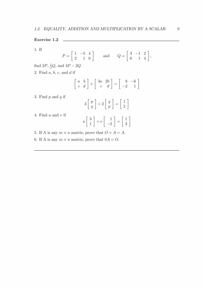
Exercise 1.2

1. If

P =

[1 −5 42 1 0

]and Q =

[3 −1 20 1 4

],

find 2P , 12Q, and 3P − 2Q.

2. Find a, b, c, and d if[a bc d

]+

[3a 2bc d

]=

[8 −6−2 1

]3. Find p and q if

3

[pq

]+ 2

[qp

]=

[12

]4. Find u and v if

u

[31

]+ v

[1−2

]=

[13

]5. If A is any m× n matrix, prove that O + A = A.

6. If A is any m× n matrix, prove that 0A = O.


1.3 Rules of Matrix Algebra (Part I)

Please read Appendix A before starting this section.

Most of the rules that we use for simplifying numerical expressions also apply whensimplifying matrix expressions. This means that most of our skills in the algebra ofnumbers will carry over to the algebra of matrices . . . but we need to know whichrules we can use and which we can not.

Rules for Matrix Addition

If A, B and C are matrices of the same size, then

(A+B) + C = A+ (B + C) (associative rule)(1.3)

A+B = B + A (commutative rule).(1.4)

These rules are the same as the rules for adding real numbers.

As with real numbers, these rules allow us to:

• write matrix sums without needing to use brackets.• rearrange the terms in a matrix sum into any order we like.

Rules for Scalar Multiplication

If A, B are matrices of the same size and if h, k are scalars, then

h(A+B) = hA+ hB (left distributive rule).(1.5)

hA+ kA = (h+ k)A (right distributive rule).(1.6)

h(kA) = (hk)A (associative rule)(1.7)

These rules allow us to

• expand brackets• simplify matrix expressions by combining like terms

in exactly the same way that we do when working with real numbers.

Examplecombininglike terms

If P and Q are matrices of the same size, simplify

P +Q+ 3Q+ 2P ,

by combining like terms.Answer

P +Q+ 3Q+ 2P = 3P + 4Q

. . . can you see where rule (1.6) was used?

1.3. RULES OF MATRIX ALGEBRA (PART I) 11

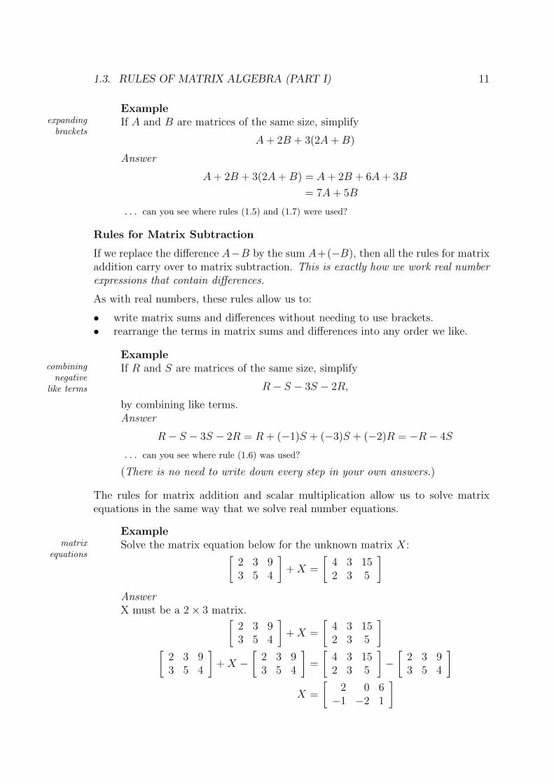
Exampleexpanding

bracketsIf A and B are matrices of the same size, simplify

A+ 2B + 3(2A+B)

Answer

A+ 2B + 3(2A+B) = A+ 2B + 6A+ 3B

= 7A+ 5B

. . . can you see where rules (1.5) and (1.7) were used?

Rules for Matrix Subtraction

If we replace the difference A−B by the sum A+(−B), then all the rules for matrixaddition carry over to matrix subtraction. This is exactly how we work real numberexpressions that contain differences.

As with real numbers, these rules allow us to:

• write matrix sums and differences without needing to use brackets.• rearrange the terms in matrix sums and differences into any order we like.

Examplecombining

negativelike terms

If R and S are matrices of the same size, simplify

R− S − 3S − 2R,

by combining like terms.Answer

R− S − 3S − 2R = R + (−1)S + (−3)S + (−2)R = −R− 4S


(There is no need to write down every step in your own answers.)

The rules for matrix addition and scalar multiplication allow us to solve matrixequations in the same way that we solve real number equations.

Examplematrix

equationsSolve the matrix equation below for the unknown matrix X:[

2 3 93 5 4

]+X =

[4 3 152 3 5

]AnswerX must be a 2× 3 matrix.[

2 3 93 5 4

]+X =

[4 3 152 3 5

][

2 3 93 5 4

]+X −

[2 3 93 5 4

]=

[4 3 152 3 5

]−[

2 3 93 5 4

]X =

[2 0 6−1 −2 1

]


ExampleSolve the matrix equation below for the unknown matrix X:[

2 11 4

]+ 2X =

[4 53 2

]Answer

X must be a 2× 2 matrix.[2 11 4

]+ 2X =

[4 53 2

][

2 11 4

]+ 2X −

[2 11 4

]=

[4 53 2

]−[

2 11 4

]2X =

[2 42 −2

]Multyiply both sides by the scalar 1

2:

1

2× 2X =

1

2

[2 42 −2

]X =

[1 21 −1

]

Note. Here we multiply both sides by 12 rather than divide both sides by 2, because mul-

tiplication by scalars has been defined and division of matrices by scalars has not been

defined!

(There is no need to write every step in these answers.)

ExampleIf A and B are matrices of the same size, solve the following equation for X:

2(X + A) + 3(B − 2X) = 4(A+B)

Answer

2(X + A) + 3(B − 2X) = 4(A+B)

2X + 2A+ 3B − 6X = 4A+ 4B

−4X = 2A+B

X = −1

4(2A+B)

Note. The answer can’t be written as − 2A+B4 because division of matrices by scalars is not

defined.

1.3. RULES OF MATRIX ALGEBRA (PART I) 13

We can prove that rules of matrix algebra are true by using the rules for real numbers.

Exampletwo

proofsProve that the associative rule for matrix addition is true.

AnswerLet A, B and C be an m× n matrices, then

(A+B) + C = ([aij] + [bij]) + [cij] = [(aij + bij) + cij]

andA+ (B + C) = [aij] + ([bij] + [cij]) = [aij + (bij + cij)].

By the associative rule for addition of real numbers:

(aij + bij) + cij = (aij + bij) + cij for each subscript i and j.

This shows that(A+B) + C = A+ (B + C).

ExampleProve that the associative rule for scalar multiplication is true.

AnswerLet h and k be scalars, and let A be an m× n matrix, then

h(kA) = h[kaij] = [h(kaij)]

and(hk)A = hk[aij] = [(hk)aij].

By the associative rule for multiplication of real numbers:

h(kaij) = (hk)aij for each subscript i and j.

This shows thath(kA) = (hk)A.

Exercise 1.3

1. If L and M are matrices of the same size, simplify.(a) L + M + 3L - 2M + L(b) 2(3L + M) - 2(M - 2L)

2. Solve the matrix equation

2(

[1 −24 3

]+ 2X)− (X − 2

[2 82 −3

]) = O


3. If R and S are matrices of the same size, solve the following equation for T :

2(R + S + T )− (2R− 3S + T ) + 3(S − T ) = O

4. Prove that the commutative rule for matrix addition is true.

1.4. MATRIX MULTIPLICATION 15

1.4 Matrix Multiplication

Matrix multiplication is more complicated than matrix addition and scalar multipli-cation, but it is very useful.

Matrix multiplication is performed by multiplying the rows of the first matrix bythe columns of the second matrix: the product of

row matrix[a b c

]and column matrix

def

is the 1× 1 matrix [ad+ be+ cf ].

Examplerow ×

column[

2 5 7] 1

42

= [2× 1 + 5× 4 + 7× 2] = [36]

When the first matrix has more than one row, each row is multiplied by the columnmatrix and the result is recorded in a separate row.

Example2 rows ×

column

[2 5 7−1 3 2

] 142

=

[2× 1 + 5× 4 + 7× 2

(−1)× 1 + 3× 4 + 2× 2

]=

[3615

]

ExampleTickets× Price

A community theatre held evening performances of a play on Fridays andSaturdays, and tickets were $30 normal price, $15 concession and $10 children.The table below shows the number of tickets sold in the first week.

Tickets Normal Concession ChildrenFriday 250 100 50Saturday 200 150 40

The ticket matrix is

T =

[250 100 50200 150 40

]and the price matrix is

P =

301510

.


• The revenue (in $) for Friday was 250 × 30 + 100 × 15 + 50 × 10 = 9500.This can also be written as

FP =[

250 100 50] 30

1510

= [9500] ,

where F =[

250 100 50]

is the Friday ticket matrix and P is the pricematrix.

• The revenue (in $) for Saturday was 200× 30 + 150× 15 + 40× 10 = 8650.This can also be written as

SP =[

200 150 40] 30

1510

= [8650] ,

where S =[

200 150 40]

is the Saturday ticket matrix and P is the pricematrix.

We can combine these calculations into a single matrix calculation to obtainthe Revenue matrix R:

R = TP =

[250 100 50200 150 40

] 301510

=

[95008650

].

Although this matrix calculation does not give us any new information, it al-lows us to organise our work in a neat compact intuitive way using the formulaRevenue = Tickets × Price. This is of practical importance when handlinglarge sets of numbers in computers.

The price matrix P was chosen to be a column vector. This choice conformswith the definition of matrix multiplication (see below). In practice you willneed to decide how information should be represented in matrices in order thatmatrices can be multiplied.

The general rule for multiplying matrices is given by:

Definition 1.4.1If A is an m× n matrix and B is an n× k matrix, then the product AB of A andB is the m× k matrix whose (i,j)-entry is calculated as follows:

multiply each entry of row i in A by the corresponding entry of column j in B,and add the results.

In other words,

AB =

row 1 of A× col 1 of B row 1 of A× col 2 of B row 1 of A× col 3 of B . . .row 2 of A× col 1 of B row 2 of A× col 2 of B row 2 of A× col 3 of B . . .

......

......

1.4. MATRIX MULTIPLICATION 17

If A and B are written in the form A = [aij] and B = [bij], then this meansAB = C = [cij] where

cij = ai1b1j + ai2b2j + ai3b3j + · · ·+ ainbnj for all i and j.

Examplemultiplying

matrices If A =

[2 1 3−1 4 5

], B =

4 51 20 3

and C =

[1 23 4

], then

(1) AB =

[row 1 of A× col 1 of B row 1 of A× col 2 of Brow 2 of A× col 1 of B row 2 of A× col 2 of B

]=

[2× 4 + 1× 1 + 3× 0 2× 5 + 1× 2 + 3× 3

(−1)× 4 + 4× 1 + 5× 0 (−1)× 5 + 4× 2 + 5× 3

]=

[9 210 18

]

(2) BC =

[row 1 of B × col 1 of C row 1 of B × col 2 of Crow 2 of B × col 1 of C row 2 of B × col 2 of Crow 3 of B × col 1 of C row 3 of B × col 2 of C

]

=

4× 1 + 5× 3 4× 2 + 5× 41× 1 + 2× 3 1× 2 + 2× 40× 1 + 3× 3 0× 2 + 3× 4

=

19 287 109 12

(3) AC is not possible. Matrix multiplication is not defined in this case asthe number of entries in a row of A is not equal to the number of entries in acolumn of B.

Example (3) above highlights an important point. In order to multiply two matrices,the number of columns in the first matrix must equal the number of rows in the secondmatrix. If A is an m× n matrix and B is an n× k matrix, then the product AB isan m× k matrix, that is

Am×nBn×k = (AB)m×k.

Exercise 1.4

1. If A =

[1 02 3

], B =

[1 −20 1

], C =

[−1 0

1 0

]and I =

[1 00 1

], calculate:

(a) OA (b) AO (c) IA (d) AI(e) AB (f) BA (g) A(BC) (h) (AB)C(i) A(B + C) (j) AB +BC

2. What is the (2, 2)-entry in the product: 1 2 34 5 67 8 9

1 2 34 5 67 8 9

.


3. If possible, calculate.

(a)

[1 −22 −3

] [32

]and

[32

] [1 −22 −3

]

(b)[

1 −2] [ 3

2

]and

[32

] [1 −2

]

1.5. RULES OF MATRIX ALGEBRA (PART II) 19

1.5 Rules of Matrix Algebra (Part II)

Please read Appendix A before starting this section.

Most - but not all - of the rules used when multiplying numbers carry over to matrixmultiplication.

The Associative Rule for Matrix Multiplication

If A, B and C are matrices which can be multiplied, then

(AB)C = A(BC)

As with real numbers, this rule allows us to write matrix products without needingto use brackets.

The Commutative Rule for Matrix Multiplication

If A and B can be multiplied, then

AB 6= BA (except in special cases)

Examplecounter-

examples If A =[

2 1], B =

[57

]and C =

[1 23 4

], then

(1) AB =[

2 1] [ 5

7

]= [17]

. . . and BA =

[57

] [2 1

]=

[10 514 7

].

(2) BC is not defined: B has order 2× 1 and C has order 2× 2.

. . . however CB =

[1 23 4

] [57

]=

[1943

].

(3) AC =[

2 1] [ 1 2

3 4

]=[

5 8]

. . . but CA is not defined: C has order 2× 2 and A has order 1× 2.

The Distributive Rules for Matrix Multiplication over Addition

If A, B and C are matrices, then

A(B + C) = AB + AC (left distribution over addition)(1.8)

(B + C)A = BA+ CA (right distribution over addition),(1.9)


(provided these sums and products make sense).

The distribution rules are also true when there are more than two terms inside thebrackets.

These rules allow us to• expand brackets, and• combine like terms together.

Examplesimplifyingexpressions

To simplify an expression like

2A(A+B)− 3AB + 4B(A−B)

we first expand brackets, then combine like terms

2A(A+B)− 3AB + 4B(A−B) = 2AA+ 2AB − 3AB + 4BA− 4BB

= 2AA− AB + 4BA− 4BB

Notice that 2AB and (−3)AB are like terms which can be combined, but that2AB and 4BA are not like terms. This is because the commutative rule is notgenerally true.

Rules for products of Scalar Multiples of Matrices

If the product A and B is defined, and if h and k are scalars, then

(1.10) (hA)(kB) = hkAB.

This rule helps us to simplify expressions by combining like terms, just as we dowhen we work with real numbers - always remembering that the ‘commutative rule’is not true for matrix multiplication.

Examplelike

termsTo simplify an expression like

2A(2A+B)− 3AB + 4B(2A−B)

we expand brackets, then combine like terms

2A(2A+B)− 3AB + 4B(2A−B) = 4AA+ 2AB − 3AB + 8BA− 4BB

= 4AA− AB + 8BA− 4BB


Exercise 1.5

Expand, then simplify the following expressions

(a) (A+B)(A−B)

(b) (A+B)(A+B)− (A−B)(A−B)

1.6. THE IDENTITY MATRICES 21

1.6 The Identity Matrices

The identity matrices are similar to the number 1 in ordinary arithmetic.

Definition 1.6.1The identity matrix of order n is the square matrix of order n with all diagonalentries equal to 1 and all other entries equal to 0, and is represented by I (or In ifit is important to emphasise the size).

I can also be written in the form I = [δij] or [δij]n, introduced in (1.2), where δij = 1when i = j and δij = 0 when i 6= j.6

Examplethe

identitymatrices

Each matrix below is an identity matrix:

I2 =

[1 00 1

], I3 =

1 0 00 1 00 0 1

, I4 =

1 0 0 00 1 0 00 0 1 00 0 0 1

, etc.

The identity matrices are similar to the number 1: if A is a m× n matrix, then

ImA = A and AIn = A.

Examplemultiplying

by anidentity

(1) If A =

[1 23 4

], then:

IA =

[1 00 1

] [1 23 4

]=

[1 23 4

]= A

and

AI =

[1 23 4

] [1 00 1

]=

[1 23 4

]= A.

. . . check these calculations.

(2) If A =

[1 2 34 5 6

], then:

I2A =

[1 00 1

] [1 2 34 5 6

]=

[1 2 34 5 6

]= A

and

AI3 =

[1 2 34 5 6

] 1 0 00 1 00 0 1

=

[1 2 34 5 6

]= A.

. . . check these calculations as well.

6δ is the Greek letter delta


1.7 Powers of Square Matrices

Matrix multiplication does not satisfy the commutative rule, so the order of mul-tiplication of two matrices is important. However, there is one special case whenthe order is not important. This is when powers of the same square matrix aremultiplied together.

Definition 1.7.1If A is a square matrix of order n, and k is a positive integer, then

Ak = AA . . . A︸︷︷︸k factors

.

You can see that if r and s are positive integers, then

ArAs = Ar+s = AsAr,

. . . so Ar and As commute.

Examplematrixpowers If A =

[1 23 4

], then

A2 = AA =

[7 10

15 22

], A3 = AA2 =

[37 5481 118

]

A4 = AA3 =

[199 290435 634

], etc . . .

Matrix powers are laborious to calculate by hand and are often calculated with spe-cial software packages such as MATLAB. Powers of matrices that satisfy polynomialequations can be found more easily.

Examplepolynomial

equationShow that the matrix

A =

[1 23 4

]satisfies the polynomial equation A2 − 5A− 2I = O, where I =

[1 00 1

]Answer

A2 − 5A− 2I =

[7 10

15 22

]− 5

[1 23 4

]− 2

[1 00 1

]=

[0 00 0

]

1.7. POWERS OF SQUARE MATRICES 23

Examplematrixpowers

If the square matrix A satisfies the polynomial equation A2 − 5A − 2I = 0,express A3 and A4 in the form rA+ sI, where r and s are scalars.

AnswerAs A2 − 5A− 2I = 0, we can write A2 = 5A+ 2I, so

A3 = AA2 = A(5A+ 2I) = 5A2 + 2A = 5(5A+ 2I) + 2A = 27A+ 10I,

and

A4 = AA3 = A(27A+ 10I) = 27A2 + 10A = 27(5A+ 2I) + 10A = 145A+ 54I.

Exercise 1.7

1. Show that A2 = O when

A =

[−2 −1

4 2

].

2. Show that B2 + 3B − 4I = O when

B =

[−1 0

3 4

]and I =

[1 00 1

].

3. If the square matrix B satisfies the equation B2 − 3B − 4I = O, express B2, B3

and B4 in the form pB + qI, where p and q are scalars.

4. Show that A3 = A when

A =

1 −1 12 0 10 2 −1

.

Explain why you can now write down the matrix A27 and A31.


1.8 The Transpose of a Matrix

So far we have looked at matrix addition, scalar multiplication and matrix multipli-cation. These were based on the operations of addition and multiplication on realnumbers. The next operation of finding the transpose of a matrix has no counterpartin real numbers.

Definition 1.8.1If A is an n × m matrix, then the transpose of A is the m × n matrix formedby interchanging the rows and columns of A, so that the first row of A is the firstcolumn of At, the second row of A is the second column of At, and so on.

If A = [aij], this means At = [aji].

Exampletaking

transposes(a) If A =

1 2 34 5 67 8 9

, then At =

1 4 72 5 83 6 9

.

(b) If B =

[1 2 34 5 6

], then Bt =

1 42 53 6

.

(c)

1 23 45 6

t

=

[1 3 52 4 6

].

(d)

123

t

=[

1 2 3].

(e)[

1 2 3]t

=

123

.

Note. Column vectors are frequently represented as transposed row vectors inprinted materials (see (e) above) in order to save space and because it’s easierto type.

Properties of Matrix transposes

• If A is a m× n matrix, then At is an n×m matrix

• If A is any matrix, then (At)t = A

• If A and B are matrices of the same size, then (A+B)t = At +Bt

• If A is an m× n matrix and B is an n× k matrix,then (AB)t = BtAt

1.8. THE TRANSPOSE OF A MATRIX 25

Exercise 1.8

1. Evaluate (a)[

1 2] [−1 3

]t(b)

[1 2

]t [ −1 3]

2. Show that (AB)t = BtAt when

A =

[1 −24 0

]and B =

[2 −1 10 2 1

].

Chapter 2

Inverses of Square Matrices

2.1 Systems of Linear Equations

The graph of the equation ax+ by = c is a straight line, so it is natural to call thisequation a linear equation in x and y. The word linear is also used when there aremore than two variables.

Many practical problems can be reduced to solving a system of linear equations.

Definition 2.1.1An equation of the form

a1x1 + a2x2 + · · ·+ anxn = b

is called a linear equation in the n variables x1, x2, . . . , xn. The numbers a1, a2,. . . , an are called the coefficients of x1, x2, . . . , xn respectively, and b is called theconstant term of the equation.

A collection of linear equations in the variables x1, x2, . . . , xn is called a systemof linear equations in these variables.

Examplea systemof linear

equations

The three equations in x1, x2 and x3

3x1 + 4x2 + x3 = 12x1 + 3x2 = 44x1 + 3x2 − x3 = −2

is a system of linear equations because each equation is a linear equation.

Note. Although the second equation has two variables, we can think of it as a linear equation

in x1, x2 and x3 with the coefficient of x3 equal to 0. In the third equation, the coefficient

of x3 is −1.

26

2.1. SYSTEMS OF LINEAR EQUATIONS 27

Examplesystem of

non-linearequations

The pair of equations4x21 + 2x2 = 4

2√x1 − 3x2 = 2

is also called a system of equations, but in this case the equations are non-linear: each variable in a linear equation must occur to the first power only.

A system of linear equations can be expressed as a single matrix equation AX = B,which may be solved using matrix ideas.


The system of equations

3x1 + 4x2 + x3 = 12x1 + 3x2 = 44x1 + 3x2 − x3 = −2

can be written as the matrix equation 3 4 12 3 04 3 −1

x1x2x3

=

14−2

,

that is, in the form AX = B, where

A =

3 4 12 3 04 3 −1

, X =

x1x2x3

and B =

14−2

,

. . . which can be solved for the unknown matrix X.

A general system of m equations in n unknowns

a11x1 + a12x2 + · · ·+ a1nxn = b1a21x1 + a22x2 + · · ·+ a2nxn = b2

......

......

am1x1 + am2x2 + · · ·+ amnxn = bm

can always be represented as a matrix equation of the form

AX = B

where

A =

a11 a12 . . . a1na21 a22 . . . a2n...

......

am1 am2 . . . amn

, X =

x1x2...xn

and B =

b1b2...bn

.

Here the matrix A is called the coefficient matrix of the system of equations.


Exercise 2.1

Write the following systems of equations in matrix form.

(a) 3x1 − x2 = 12x1 + 3x2 = 4

(b) 3x1 + 4x2 − 5x3 = 12x1 − x2 + 3x3 = 0

(c) 4x2 + x3 = 12x1 − x3 = −14x1 + 3x2 = 2

2.2. THE INVERSE OF A SQUARE MATRIX 29

2.2 The Inverse of a Square Matrix

The matrix equation AX = B is very similiar to the linear equation ax = b, wherea and b are numbers. This linear equation is solved by multiplying both sides by1/a = a−1, the reciprocal or inverse of a:

ax = ba−1ax = a−1b

1x = a−1bx = a−1b

The same technique can be used for solving matrix equations of the form AX = B. . . once the inverse of a matrix is defined

If a is any number, then its inverse is that special number p for which pa = ap = 1.For example, the inverse of 2 is 0.5 as 0.5 × 2 = 2 × 0.5 = 1. We traditionallyrepresent the inverse of a by the special symbol a−1, for example 2−1 = 0.5. Thesesame ideas can carried over to matrices.

In matrix theory, identity matrices are used to define inverses of square matrices.

Definition 2.2.1Let A and P be n× n matrices. If

(2.1) PA = AP = I,

where I is the n × n identity matrix, then P is called the inverse of A and isrepresented by the special symbol A−1. So

(2.2) A−1A = AA−1 = I.

If A has an inverse, then A is said to be invertible.

You can see from this definition that if P is the inverse of A, then A is the inverseof P . We can write this in symbols as P−1 = A or as

(2.3) (A−1)−1 = A.

Examplean

invertiblematrix

Show that

[2 51 3

]−1

=

[3 −5−1 2

]Answer

If A =

[2 51 3

]and P =

[3 −5−1 2

], then

PA =

[3 −5−1 2

] [2 51 3

]=

[1 00 1

]= I,


and

AP =

[2 51 3

] [3 −5−1 2

]=

[1 00 1

]= I

so P is the inverse of A . . . and A is the inverse of P .

If A has an inverse, then the matrix equation AX = B can be solved as follows:

AX = BA−1AX = A−1B

IX = A−1B . . . as A−1A = I in (2.2)X = A−1B

Examplesolving

a matrixequation

Write the pair of simultaneous equations

2x+ 5y = 7x+ 3y = 4

as a matrix equation, then solve this matrix equation.AnswerThe matrix equation is [

2 51 3

] [xy

]=

[74

].

We saw in the previous example that[2 51 3

]−1

=

[3 −5−1 2

],

so [3 −5−1 2

] [2 51 3

] [xy

]=

[3 −5−1 2

] [74

][

1 00 1

] [xy

]=

[3 −5−1 2

] [74

][xy

]=

[11

]The matrix equation AX = B can always be solved if A has an inverse . . . but notall square matrices are invertible (ie. have inverses).

Examplea non-

invertiblematrix

The pair of simultaneous equations

2x+ 5y = 72x+ 5y = 6

2.2. THE INVERSE OF A SQUARE MATRIX 31

does not have a solution, so the matrix equation[2 52 5

] [xy

]=

[76

]does not have a solution. This means that the coefficient matrix[

2 52 5

]does not have an inverse, and so is not invertible.

If a and b are numbers, then the reciprocal or inverse of the product ab is

(ab)−1 = a−1b−1

. . . however this is not true for matrices.

Exampleinverse

of matrixproduct

If A and B are n× n matrices, show that

(AB)−1 = B−1A−1.

AnswerWe are asked to show that the inverse of AB is B−1A−1. To do this we needto show that condition (2.2) in Definition 2.2.1 is satisfied.

It can be confusing when a problem uses the same letters that are in a definition. The wayto overcome this is to express the definition in words. In this case, condition (2.2) says:(1) when a matrix is multiplied on the the left by its inverse, the result is the identity matrix,(2) when a matrix is multiplied on the right by its inverse, result is the identity matrix again.

. . . we need to check that (1) and (2) are true for AB and B−1A−1.

(1) Multiplying AB on the left by B−1A−1:

(B−1A−1)(AB) = B−1A−1AB . . . as there’s no need to use brackets

= B−1IB . . . as A−1A = I

= BB−1 . . . as IB = B

= I . . . as BB−1 = I

(2) Multiplying AB on the right by B−1A−1:

(AB)(B−1A−1) = ABB−1A−1 . . . as there’s no need to use brackets

= AIA−1 . . . as BB−1 = I

= AA−1 . . . as AI = A

= I . . . as AA−1 = I

This shows that (AB)−1 = B−1A−1.

Note. (AB)−1 = B−1A−1 6= A−1B−1 as the commutative law is not true for matrix multi-

plication except in special cases.


Exercise 2.2

1. Show that V = 13

12 −13 −7−3 5 2−3 2 2

is the inverse of U =

2 4 30 1 −13 5 7

.

2. Show that

[3 24 3

]−1

=

[3 −2−4 3

]3. Use your answer to question 2 to solve the following:

(a) The simultaneous equations:

3x+ 2y = 44x+ 3y = 7

(b) The matrix equation AX = B, when

A =

[3 24 3

]and B =

[1 24 −2

].

(c) The matrix equation PX = Q, when

P =

[3 −2−4 3

]and Q =

[0 −1 2−2 1 −1

].

4. A is a square matrix that satisfies A2 − 3A + I = O, where I is the identitymatrix. Show that A has an inverse.

5. If A, B and C are invertible square matrices of order n, show that ABC isinvertible and the inverse is C−1B−1A−1.

6. If A is an invertible n× n matrix, then the negative integer powers of A can bedefined as

A−k = A−1A−1 . . . A−1︸︷︷︸k factors

,

where k is a positive integer. Show that (A2)−1 = A−2.

Note. If A0 is defined to be the identity matrix In, the power rules ArAs = Ar+s and (Ar)s = Ars

are true for all integers r and s.

2.3. INVERSES OF 2× 2 MATRICES 33

2.3 Inverses of 2× 2 Matrices

The matrix equation AX = B can be solved when A is invertible. It is importantto decide which square matrices have inverses and how to calculate these inverses.

TheoremIf A is a 2× 2 matrix, then A is invertible if and only if 1

(2.4) a11a22 − a12a21 6= 0,

and, when this condition is true, the inverse is

(2.5) A−1 =1

a11a22 − a12a21

[a22 −a12−a21 a11

].

Exampleinvertible

matrixThe matrix [

3 52 4

]has an inverse because 3× 4− 5× 2 = 2 6= 0. The inverse is[

3 52 4

]−1

=1

2

[4 −5−2 3

]

Exampleinvertibility For what values of k is the matrix

T =

[3 k2 4

]invertible?AnswerT is invertible if and only if 3× 4− k × 2 6= 0, that is if and only if k 6= 6.

The number a11a22 − a12a21 is very important, as it tells us when A is invertible.

Definition 2.3.1If A is a 2 × 2 matrix, then the number a11a22 − a12a21 is called the determinantof A. It is represented by the special symbols detA and |A|.2

Properties of Determinants

• If A is a 2× 2 matrix, then A is invertible if and only if detA 6= 0

• If A and B are 2× 2 matrices, then det(AB) = detA detB

1See page 5, footnote 12We will use the symbol detA in this topic.


Examplematrix

product Let A = det

[3 52 4

]and B = det

[1 23 4

], then detA = 2 and detB = −2.

As AB =

[3 52 4

] [1 23 4

]=

[18 2614 20

], we can see that det(AB) = −4.

This is an example of det(AB) = detA detB.

Examplematrixpowers

Let A be a 2× 2 matrix. Show that det(A2) = (detA)2.AnswerAs A2 = AA, det(A2) = detAA = detA detA = (detA)2.


detA = a11a22a33 + a12a23a31 + a13a21a32 − a13a22a31 − a11a23a32 − a12a21a33You can avoid memorising this formula by using the pictures below:

(a)

@@@@@@R

��

��

��

a11 a12

a21a22

(b)

@@@@@@@@R

@@@@@@@@R

@@@@@@@@R

��

��

��

��

��

��

��

��

��

a31 a32 a33

a21 a22 a23

a11 a12 a13

a31 a32

a21 a22

a11 a12

The formula for a 2 × 2 determinant is obtained from diagram (a) by multiplyingthe terms on each arrow together, then subtracting those on the arrows going fromleft to right from those on the arrow going from right to left. The formula for a 3×3determinant is obtained from diagram (b) similarly.

The formula for a general n× n determinant can be obatined by writing the matrixdown twice, with the copy along side the original as in (b), drawing n arrows goingfrom left to right and n arrows going from right to left as in (b), then continuing asin the 3× 3 case.

There is a general formula for the inverse of a square matrix of order n, but thecalculation takes a lot of time and a more efficient method is shown in the nextsection.

Exercise 2.3


A =

[1 23 4

].

2.3. INVERSES OF 2× 2 MATRICES 35

2. Let A be a matrix of order 2 with inverse A−1. Use the properties of determinantsto show that det(A−1) = 1/ detA

3. Let A be a matrix of order 2 for which A2 = 0. Use the properties of determinantsto show that A does not have an inverse.

4. Evaluate detA, where

A =

1 2 −33 1 10 1 −2

.

Is A invertible?


2.4 Calculating the Inverse of an n× n Matrix

The most efficient way of calculating the inverse of a square matrix is to use eleme-natry row operations.

This is best shown by example on a 3× 3 matrix: To find the inverse of

A =

2 7 11 4 −11 3 0

,

construct the augmented-matrix [A|I] from A and the identity matrix I of order 3:

[A|I] =

2 7 1 1 0 01 4 −1 0 1 01 3 0 0 0 1

,

then use elementary row operations to convert this into the form [I|B], having theidentity matrix of order 3 in the first three columns:

[I|B] =

1 0 0 b11 b12 b130 1 0 b21 b22 b230 0 1 b31 b32 b33

.

If you can do this, then the matrix B is the inverse of A. If you can not, then Adoes not have an inverse.

There are three elementary row operations which can used for this procedure.

Elementary Row Operations(1) Interchange two rows.(2) Multiply or divide one row by a non-zero number.(3) Add a multiple of one row to another row.

To keep track of the our operations, we use the notation:

(1) Ri � Rj to mean interchange row i and row j.(2) Ri → cRi to mean replace row i by row i multiplied by c.(3) Rj → Rj + cRi to mean to add row i multiplied by c to row j.

Examplecalculatingthe inverse

matrix

To change the augmented matrix 2 7 1 1 0 01 4 −1 0 1 01 3 0 0 0 1

into the form [I|B]

• interchange row 1 and row 2, so that the (1, 1)-entry becomes 1.

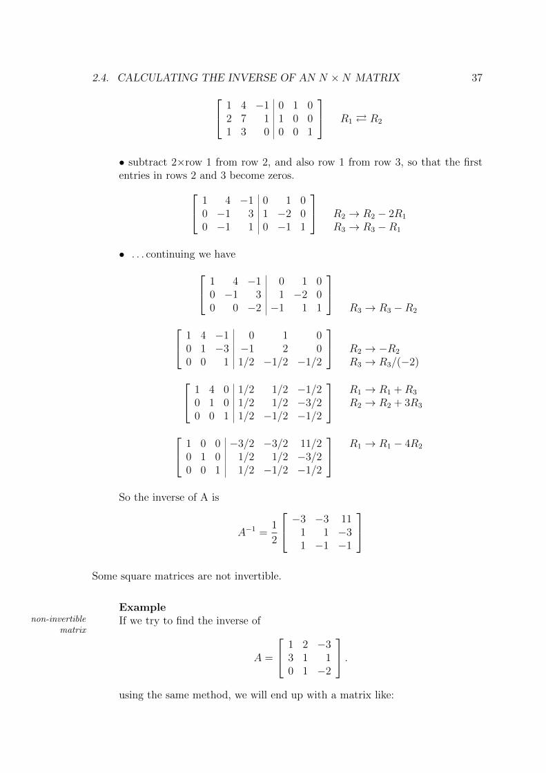
2.4. CALCULATING THE INVERSE OF AN N ×N MATRIX 37 1 4 −1 0 1 02 7 1 1 0 01 3 0 0 0 1

R1 � R2

• subtract 2×row 1 from row 2, and also row 1 from row 3, so that the firstentries in rows 2 and 3 become zeros. 1 4 −1 0 1 0

0 −1 3 1 −2 00 −1 1 0 −1 1

R2 → R2 − 2R1

R3 → R3 −R1

• . . . continuing we have 1 4 −1 0 1 00 −1 3 1 −2 00 0 −2 −1 1 1

R3 → R3 −R2 1 4 −1 0 1 0

0 1 −3 −1 2 00 0 1 1/2 −1/2 −1/2

R2 → −R2

R3 → R3/(−2) 1 4 0 1/2 1/2 −1/20 1 0 1/2 1/2 −3/20 0 1 1/2 −1/2 −1/2

R1 → R1 +R3

R2 → R2 + 3R3

1 0 0 −3/2 −3/2 11/20 1 0 1/2 1/2 −3/20 0 1 1/2 −1/2 −1/2

R1 → R1 − 4R2

So the inverse of A is

A−1 =1

2

−3 −3 111 1 −31 −1 −1

Some square matrices are not invertible.

Examplenon-invertible

matrixIf we try to find the inverse of

A =

1 2 −33 1 10 1 −2

.

using the same method, we will end up with a matrix like:


1 2 −3 1 0 00 1 −2 −3/5 −1/5 00 0 0 3/5 1/5 1

.

The row of zeros in the first part of this matrix shows that it is impossible toobtain a matrix in the form [I|B] where I is the identity matrix of order 3.This implies that A does not have an inverse.

Exercise 2.4

If possible, find the inverse of the following matrices using elementary row transfor-mations.

(a)

[2 31 4

](b)

[1 22 4

]

(c)

3 1 −15 2 01 1 −1

(d)

1 0 11 1 −12 1 0

Appendix A

The Algebra of Numbers

Many of the rules that we use to evaluate or simplify real number expressions canalso be used with matrices. These rules are explained below.

Associative Rules for Addition and Multiplication

The associative rules show that if three numbers are added or multiplied, then itdoesn’t matter how you do this, the answer is always the same.

If a, b and c are real numbers, then

(a+ b) + c = a+ (b+ c) (addition)(A.1)

(ab)c = a(bc) (multiplication)(A.2)

Examplecombining

threenumbers

When three numbers are added or multiplied, there is more than one way ofdoing this:

adding 2, 3 and 4⇒{

(2 + 3) + 4 = 5 + 4 = 92 + (3 + 4) = 2 + 7 = 9

multiplying 2, 3 and 4⇒{

(2× 3)× 4 = 6× 4 = 242× (3× 4) = 2× 12 = 24

The answer is the same in each case, and this is what the associative rules foraddition and multiplication describe.

As there is no difference in the answers, there is no need to use brackets whenadding or multiplying 3 numbers together . . . we can just write 2 + 3 + 4 and2× 3× 4.

The associative rules show that there is no need to use brackets in sums or productsof three numbers. This is also true for sums and products with any number of terms.

We use the associative rules every time we write sums and products without usingbrackets.

39

40 APPENDIX A. THE ALGEBRA OF NUMBERS

Examplewritingwithout

brackets

We don’t usually use brackets when writing:

• sums like 2x+ 3y + 4x+ 5z + 7y• products like x2y3x4z5y7

Commutative Rules for Addition and Multiplication

The commutative rules show that the order in which 2 numbers are added or mul-tiplied doesn’t matter, the answer is always the same.

If a and b are real numbers, then

a+ b = b+ a (addition)(A.3)

ab = ba (multiplication)(A.4)

Examplechangingthe order

When two numbers are added or multiplied, there is more than one way ofdoing this:

adding 3 to 2 ⇒ 2 + 3 = 5adding 2 to 3 ⇒ 3 + 2 = 5

multiplying 2 by 3 ⇒ 2× 3 = 6multiplying 3 by 2 ⇒ 3× 2 = 6

The answer is the same in each case, and this is what the commutative rulesfor addition and multiplication describe.

We use the associative and commutative rules every time we rearrange sums andproducts of real numbers, for example when collecting like terms together or whensimplifying products.

Examplecollecting

like termsTo simplify a sum like

2x+ 3y + 4x+ 5z + 7y,

we first collect like terms together:

2x+ 3y + 4x+ 5z + 7y = 2x+ 4x+ 3y + 7y + 5z = etc . . .

Examplerearranging

powersTo simplify a product like

x2y3x4z5y7,

we need to combine powers with the same base:

x2y3x4z5y = x2x4y3y7z5 = etc . . .

41

Distributive Rules for Multiplication over Addition

The distributive rules describe how we expand brackets and how we factorise.

If a, b and c are real numbers, then

a(b+ c) = ab+ ac (left distribution)(A.5)

(b+ c)a = ba+ ca (right distribution)(A.6)

The distribution rules are also true when there are more than two terms inside thebrackets. We use these rules every time we expand brackets and every time wesimplify sums by combining like terms together.

Exampleexpanding

andsimplifying

To simplify a sum like

2(x+ y) + 4(2x+ z) + 7y,

we first expand brackets, then combine like terms:

2(x+ y) + 4(2x+ z) + 7y = 2x+ 2y + 8x+ 4z + 7y = 10x+ 9y + 4z

. . . can you see where the left distributive rule (A.5) was used . . . and the right distributive

rule (A.6)?

Exampleexpanding

bracketsTo expand a product like

(x+ 2)(x+ 3),

we multiply out the brackets like this

(x+ 2)(x+ 3) = x(x+ 3) + 2(x+ 3) = x2 + 3x+ 2x+ 6 = x2 + 5x+ 6

. . . can you see where the left distributive rule (A.6) was used . . . and the two places

where the right distributive rule (A.5) was used?

Rules for Subtraction and Division

In order to use algebra to manipulate expressions involving subtraction and division,we first need to talk about negatives and reciprocals.

The negative of a number a is the unique number (denoted by −a) such that

a+ (−a) = (−a) + a = 0.

Now the difference between two numbers can be rewritten as the sum of the firstand the negative of the second, and we can apply the rules of addition above to thissum.

42 APPENDIX A. THE ALGEBRA OF NUMBERS

If a and b are real numbers, then

(A.7) a− b = a+ (−b) = a+ (−1)b.

This means that we can use the associative and commutative rules for additionwhen we rearrange sums and differences of real numbers, provided that differencesare interpreted as in (A.7).rearranging

sums anddifferences

Example

To simplify an expression like

2x− 3y + 4x− 5z + 7y,

we write

2x− 3y + 4x− 5z + 7y = 2x+ 4x− 3y + 7y − 5z = 6x+ 4y − 5z

because we know

2x+ (−3y) + 4x+ (−5z) + 7y = 2x+ 4x+ (−3)y+ 7y+ (−5z) = 6x+ 4y− 5z.

The reciprocal of a number a is the unique number (denoted a−1) such that

a× a−1 = a−1 × a = 1.

Now the quotient of two numbers can be rewritten as a product of the numeratorwith the reciprocal of the denominator, so the rules for products above can beapplied.

If a and b 6= 0 are real numbers, then

a

b= a× b−1

However, we need to be careful when dividing numbers, as the associative rule andthe commutative rule are not true for division!

Example

(24÷ 6)÷ 2 = 4÷ 2 = 2 and 24÷ (6÷ 2) = 24÷ 3 = 8.

6÷ 2 = 3 and 2÷ 6 =1

3

Appendix B

Answers

Exercise 1.1

1(a) pq (b) q (c) p 2(a) −2 (b) y (c) 0 (d) −3

3. A =

[a11 a12 a13a21 a22 a23

]4. B =

020

5. C =

2 33 44 5

Exercise 1.2

1.

[2 −10 84 2 0

],

[3/2 1/2 1

0 1/2 2

],

[−3 −13 8

6 1 −8

]2. a = 2, b = −2, c = −1, and d = 1

23. p = −1

5, q = 4

54. u = 5

7, v = −8

7

5. & 6. Check with a tutor.

Exercise 1.3

1(a) 5L−M (b) 10L 2. X = −[

2 44 0

]3. T = 4S

4. Check with a tutor.

Exercise 1.4

1(a)

[0 00 0

](b)

[0 00 0

](c)

[1 02 3

](d)

[1 02 3

](e)

[1 −22 −1

](f)

[−3 −6

2 3

](g)

[−3 0−3 0

](h)

[−3 0−3 0

](i)

[0 −23 −1

](j)

[−2 −2

3 −1

]2. 81

3(a)

[−1

0

]; not possible (b) [−1];

[3 −62 −4

]

43

44 APPENDIX B. ANSWERS

Exercise 1.5

(a) A2 − AB +BA−B2 (b) 2AB + 2BA

Exercise 1.7

3.B2 = 3B + 4I, B3 = 13B + 12I, B4 = 51B + 52I

4. A9 = (A3)3 = (A)3 = A =⇒ A27 = (A9)3 = (A)3 = Aand A31 = A27A3A = AAA = A3 = A

Exercise 1.8

1(a) [5] (b)

[−1 3−2 6

]Exercise 2.1

(a)

[3 −12 3

] [x1x2

]=

[14

](b)

[3 4 −52 −1 3

] x1x2x3

=

[10

]

(c)

0 4 12 0 −14 3 0

x1x2x3

=

1−1

2

Exercise 2.2

3(a)

[xy

]=

[−2

5

](b) X =

[−5 10

8 −14

](c) X =

[−4 −1 4−6 −1 5

]4. A−1 = 3I − A 5. & 6. Check with a tutor.

Exercise 2.3

1. −12

[4 −2−3 1

]2 & 3. Check with a tutor. 4. 0; no

Exercise 2.4

(a) 15

[4 −3−1 2

](b) not possible

(c) 14

2 0 −2−5 2 5−3 2 −1

(d) not possible

matr ix mathstrack here the matrix - university of … · 2.4 calculating the inverse of an n ! n...

Documents