METU, 2015 Prepared by Derya Kaya

MATLAB TUTORIAL

1) Matlab Panels

2) Operations and Variables

3) Matrices

4) Scripts

5) Plotting

6) Simulink

METU, 2015 Prepared by Derya Kaya

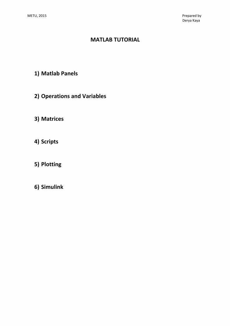
1) Matlab panels:

Command Window Command History

Workspace

Current Folder

Current Folder: You can access your files.

Command Window: You can enter the commands after the >> sign.

Workspace: Data that you create or import are explored here.

Command History: Return the commands that you enter at the command line. To clear the Command History

click right on it then click “Clear Command History”.

Matlab has an online documentation facility. You can access it by help or doc command (e.g. >> help sin)

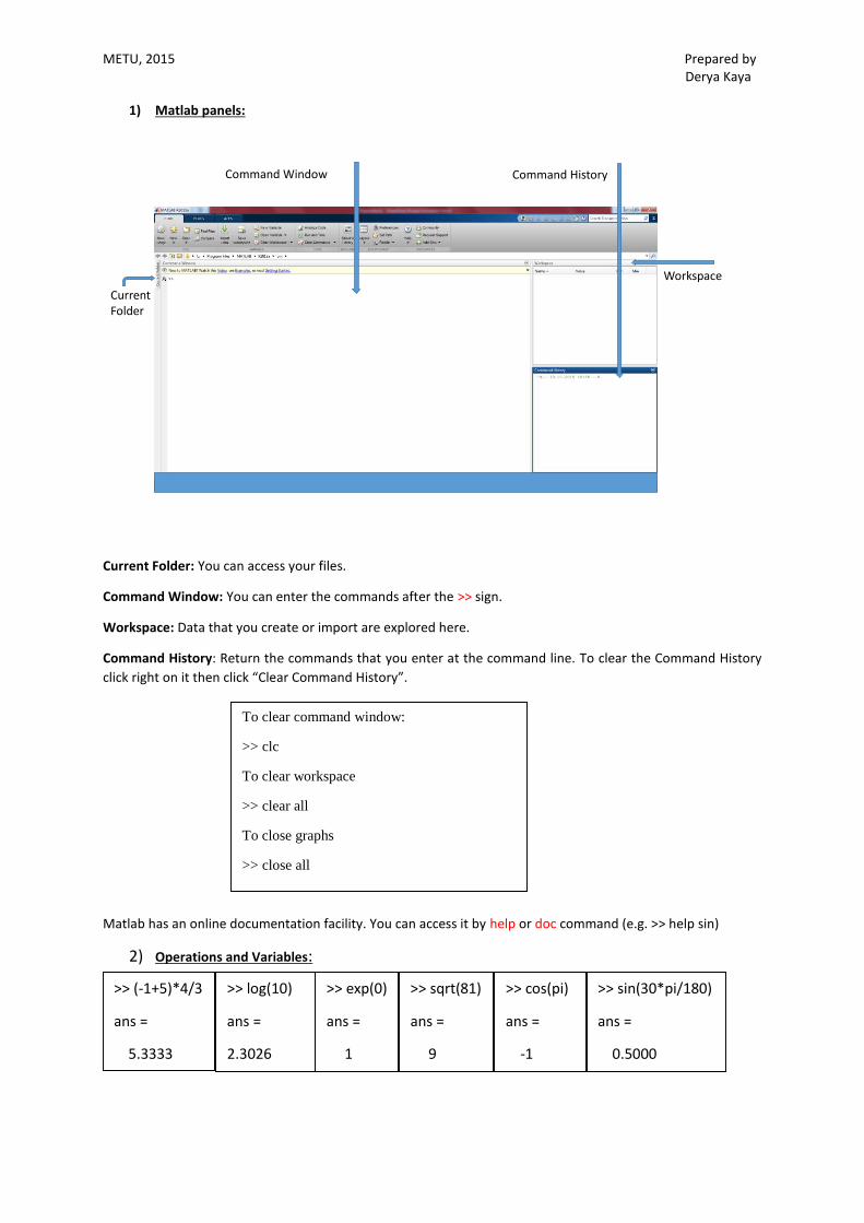
2) Operations and Variables:

>> log(10)

ans =

2.3026

>> exp(0)

ans =

1

>> sqrt(81)

ans =

9

>> cos(pi)

ans =

-1

>> sin(30*pi/180)

ans =

0.5000

>> (-1+5)*4/3

ans =

5.3333

To clear command window:

>> clc

To clear workspace

>> clear all

To close graphs

>> close all

METU, 2015 Prepared by Derya Kaya

You can also use j to indicate the complex numbers. pi has the value 3.14159..

Inside the cos, sin, tan, atan, etc. commands, you should write the angle in terms of radian. So, convert the

degree to radian!

In Matlab, you should define the variables. Otherwise it giver error!

If the variables that you want to use do not have a specific value, then you should define them as a symbolic

function by syms command.

>> a=3;b=2;a+b

ans =

5

When you put the ; at the end of the

command it still define the variable

and write to the workspace. In order

to get a clear command window use ;

at the end of the commands.

Y = ceil(X) rounds each element of X to the nearest integer greater than or equal to that element.

Y = floor(X) rounds each element of X to the nearest integer less than or equal to that element.

Y = round(X) rounds each element of X to the nearest integer. In the case of a tie, where an element

has a fractional part of exactly 0.5, the round function rounds away from zero to the integer with

larger magnitude.

Reference: http://www.mathworks.com/help/matlab/ref/round.html

>> a+1

Undefined

function or

variable 'a'.

a =

3

>> a+1

ans =

4

>> 5^2

ans =

25

>> i^2

ans =

-1

>>

abs(i+1)

ans =

1.4142

>> sqrt(2)

ans =

1.4142

>>

angle(i+1)

*180/pi

ans =

45

>> sin(30*pi/180)

ans =

0.5000

METU, 2015 Prepared by Derya Kaya

Cleaning up symbolic statements:

>> simplify (ans) simplifies ans

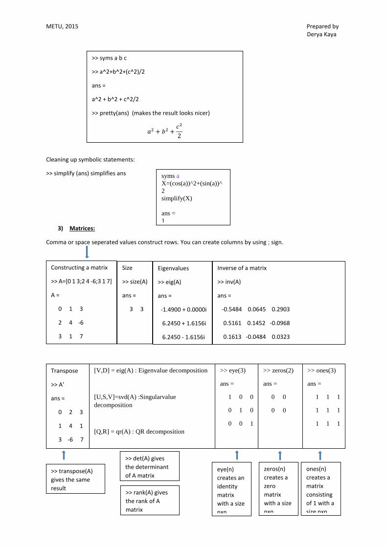
3) Matrices:

Comma or space seperated values construct rows. You can create columns by using ; sign.

To do elementwise operations use dot (e.g. A./B or A.*B).

>> syms a b c

>> a^2+b^2+(c^2)/2

ans =

a^2 + b^2 + c^2/2

>> pretty(ans) (makes the result looks nicer)

𝑎2 + 𝑏2 +𝑐2

2

Constructing a matrix

>> A=[0 1 3;2 4 -6;3 1 7]

A =

0 1 3

2 4 -6

3 1 7

Size

>> size(A)

ans =

3 3

Eigenvalues

>> eig(A)

ans =

-1.4900 + 0.0000i

6.2450 + 1.6156i

6.2450 - 1.6156i

Inverse of a matrix

>> inv(A)

ans =

-0.5484 0.0645 0.2903

0.5161 0.1452 -0.0968

0.1613 -0.0484 0.0323

Transpose

>> A'

ans =

0 2 3

1 4 1

3 -6 7

[V,D] = eig(A) : Eigenvalue decomposition

[U,S,V]=svd(A) :Singularvalue

decomposition

[Q,R] = qr(A) : QR decomposition

>> eye(3)

ans =

1 0 0

0 1 0

0 0 1

>> zeros(2)

ans =

0 0

0 0

>> ones(3)

ans =

1 1 1

1 1 1

1 1 1

eye(n)

creates an

identity

matrix

with a size

nxn

zeros(n)

creates a

zero

matrix

with a size

nxn

ones(n)

creates a

matrix

consisting

of 1 with a

size nxn

>> transpose(A)

gives the same

result

>> det(A) gives

the determinant

of A matrix

>> rank(A) gives

the rank of A

matrix

syms a

X=(cos(a))^2+(sin(a))^

2

simplify(X)

ans =

1

METU, 2015 Prepared by Derya Kaya

Elementwise operation

4) Scripts

To create a new editor document, write >> edit at the command line or click to the “New Script” as shown in the

following figure.

Why do we use editor (m file)?

To make changes on it

To save and use it later

First row of A

matrix

Third column

of A matrix

>> A=[1 2 3;4 5 6]

A =

1 2 3

4 5 6

>> A(1,3)

ans =

3

>> A(2,2)

ans =

5

A =

1 2 3

4 5 6

>> B=A(1,:)

B =

1 2 3

>> C=A(:,3)

C =

3

6

>> a=[1 2];b=[3 4];c=[a;b]

c =

1 2

3 4

>> d=[a b]

d =

1 2 3 4

>> B=[ones(2);1 -4]

B =

1 1

1 1

1 -4

>> B(6)

ans =

-4

C = rand(n) returns an n-

by-n matrix of random

numbers.

>> C=rand(2)

C =

0.8235 0.3171

0.6948 0.9502

>> A=[1 2;3 4];

>> B=[5 6;7 8];

>> A*B

ans =

19 22

43 50

>> A.*B

ans =

5 12

21 32

METU, 2015 Prepared by Derya Kaya

New Script

* means that it is not saved. Save the file and then press the Run button

Anything following percent sign (%) is a comment! Comments helps you to understand the code when you use it

later. Hence, you can save your time.

You cannot run the commands that you write to the editor unless you don’t save it!

METU, 2015 Prepared by Derya Kaya

5) Plotting

y = linspace(n,m) returns a row vector of 100 evenly spaced points between n and m.

y = linspace(n,m,k) generates n points. The spacing between the points is (m-n)/(k-1).

2D Plotting:

You need to write axes names and put a title and/or legend.

>> x=linspace(1,5);

>> y=sin(x);

>> plot(x,y)

x and y vectors must be same size.

Otherwise you get an error!

>> x=linspace(1,5); >> y=sin(x); >> plot(x,y) >> xlabel('RPM') >> ylabel('Thrust') >> title('Angular velocity versus thrust') >> legend('A')

1 1.5 2 2.5 3 3.5 4 4.5 5

-1

-0.8

-0.6

-0.4

-0.2

0

0.2

0.4

0.6

0.8

1

1 1.5 2 2.5 3 3.5 4 4.5 5

-1

-0.8

-0.6

-0.4

-0.2

0

0.2

0.4

0.6

0.8

1

RPM

Thru

st

Angular velocity versus thrust

A

>> t=(1:5)

t =

1 2 3 4 5

>> t=(1:0.5:5)

t =

1.0000 1.5000 2.0000 2.5000

3.0000 3.5000 4.0000 4.5000

5.0000

t(n:m) creates a vector from n to m

with 1 increment

t(n:k:m) creates a vector from n to m

with k increment

METU, 2015 Prepared by Derya Kaya

You can also insert x label, y label, title or legend by clicking on the insert part on the graph.

Insert x label, y label, title, legend, etc.

plot(x,y,'r.-')

Color Marker Line

Style

1 1.5 2 2.5 3 3.5 4 4.5 5

-1

-0.8

-0.6

-0.4

-0.2

0

0.2

0.4

0.6

0.8

1

RPM

Thru

st

Angular velocity versus thrust

A

x=linspace(1,5);

y=sin(x);

plot(x,y,'g*-')

hold on

z=cos(x)

plot(x,z,'r*')

xlabel('RPM')

ylabel('Thrust')

title('Omega versus thrust')

legend('y=sin(x)','z=cos(x)','Location','southwes

t')

1 1.5 2 2.5 3 3.5 4 4.5 5-1

-0.8

-0.6

-0.4

-0.2

0

0.2

0.4

0.6

0.8

1

RPM

Thru

st

Omega versus thrust

y=sin(x)

z=cos(x)

METU, 2015 Prepared by Derya Kaya

Specifier Line Style

- Solid line (default)

-- Dashed line

: Dotted line

-. Dash-dot line

Specifier Marker

o Circle

+ Plus sign

* Asterisk

. Point

x Cross

s Square

d Diamond

^ Upward-pointing triangle

v Downward-pointing triangle

> Right-pointing triangle

< Left-pointing triangle

p Pentagram

h Hexagram

Specifier Color

y yellow

m magenta

c cyan

r red

g green

b blue

w white

k black

METU, 2015 Prepared by Derya Kaya

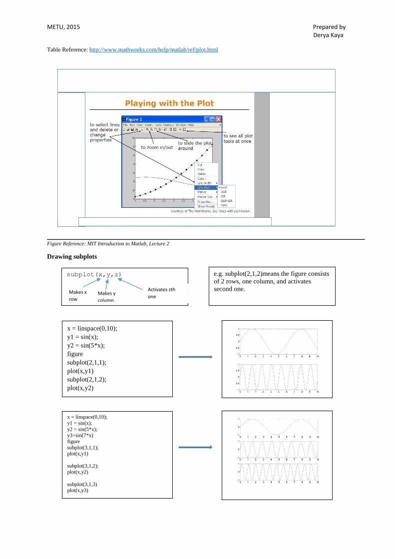
Table Reference: http://www.mathworks.com/help/matlab/ref/plot.html

Figure Reference: MIT Introduction to Matlab, Lecture 2

Drawing subplots

x = linspace(0,10);

y1 = sin(x);

y2 = sin(5*x);

figure

subplot(2,1,1);

plot(x,y1)

subplot(2,1,2);

plot(x,y2)

x = linspace(0,10);

y1 = sin(x);

y2 = sin(5*x); y3=sin(7*x)

figure

subplot(3,1,1); plot(x,y1)

subplot(3,1,2); plot(x,y2)

subplot(3,1,3) plot(x,y3)

subplot(2,1,2);

subplot(x,y,z)

Makes x

row Makes y

column

Activates zth

one

e.g. subplot(2,1,2)means the figure consists

of 2 rows, one column, and activates

second one.

METU, 2015 Prepared by Derya Kaya

>> close all command closes all figures.

>>close[n m] command closes nth and mth figures.

3D Plotting:

Surface and mesh plots

>> time=(0:0.4:10);

>> z=time;

>> x=sin(time);

>> y=cos(time);

>> plot3(x,y,z,'b','Linewidth',2)

x=-pi:0.1:pi; y=-pi:0.1:pi; [a,b]=meshgrid(x,y); % to make

matrices Z=sin(a).*cos(b); surf(x,y,Z)

x=-pi:0.1:pi; y=-pi:0.1:pi; [a,b]=meshgrid(x,y); % to make

matrices c=sin(a).*cos(b); contour(a,b,c)

METU, 2015 Prepared by Derya Kaya

6) Simulink

Open new document

Simulink library browser includes various blocks that you need.

Example: Mass-spring-damper

References:

Introduction to Programing in Matlab, MIT opencourseware

http://www.mathworks.com/help/matlab/ref/plot.html