matlab program for precision calibration of optical tweezers program for... · computer physics...

c

xperimenttheonachievedpositionEinstein–uess for

pendencequencysed byarameters.used for

lues,

b

ct

Computer Physics Communications 159 (2004) 225–240

www.elsevier.com/locate/cp

MatLab program for precision calibration of optical tweezers✩

Iva Marija Tolic-Nørrelykkea,1, Kirstine Berg-Sørensena,∗, Henrik Flyvbjergb

a The Niels Bohr Institute, Blegdamsvej 17, DK-2100 Copenhagen Ø, Denmarkb Plant Research Department and Danish Polymer Centre,Risø National Laboratory, DK-4000 Roskilde, Denmark

Received 1 June 2003; accepted 24 February 2004

Abstract

Optical tweezers are used as force transducers in many types of experiments. The force they exert in a given eis known only after a calibration. Computer codes that calibrate optical tweezers with high precision and reliability in(x, y)-plane orthogonal to the laser beam axis were written in MatLab (MathWorks Inc.) and are presented here. The calibratiis based on the power spectrum of the Brownian motion of a dielectric bead trapped in the tweezers. Precision isby accounting for a number of factors that affect this power spectrum. First, cross-talk between channels in 2Dmeasurements is tested for, and eliminated if detected. Then, the Lorentzian power spectrum that results from theOrnstein–Uhlenbeck theory, is fitted to the low-frequency part of the experimental spectrum in order to obtain an initial gparameters to be fitted. Finally, a more complete theory is fitted, a theory that optionally accounts for the frequency deof the hydrodynamic drag force and hydrodynamic interaction with a nearby cover slip, for effects of finite sampling fre(aliasing), for effects of anti-aliasing filters in the data acquisition electronics, and for unintended “virtual” filtering cauthe position detection system. Each of these effects can be left out or included as the user prefers, with user-defined pSeveral tests are applied to the experimental data during calibration to ensure that the data comply with the theorytheir interpretation: Independence ofx- and y-coordinates, Hooke’s law, exponential distribution of power spectral vauncorrelated Gaussian scatter of residual values. Results are given with statistical errors and covariance matrix.

Program summary

Title of program: tweezercalibCatalogue identifier:ADTVProgram obtainable from:CPC Program Library, Queen’s University of Belfast, N. Ireland.Program Summary URL:http://cpc.cs.qub.ac.uk/summaries/ADTVComputer for which the program is designed and others on which it has been tested:General computer running MatLa(MathWorks Inc.).Programming language used:MatLab (MathWorks Inc.). Uses “Optimization Toolbox” and “Statistics Toolbox”.

✩ This paper and its associated computer program are available viathe Computer Physics Communications homepage on ScienceDire(http://www.sciencedirect.com/science/journal/00104655).

* Corresponding author.E-mail address:[email protected] (K. Berg-Sørensen).

1 Permanent address: Rugjer Boškovic Institute, Bijenicka 54, HR-10000 Zagreb, Croatia.

0010-4655/$ – see front matter 2004 Elsevier B.V. All rights reserved.doi:10.1016/j.cpc.2004.02.012

http://www.elsevier.com/locate/cpc

http://cpc.cs.qub.ac.uk/summaries/ADTV

http://www.sciencedirect.com/science/journal/00104655

226 I.M. Tolic-Nørrelykke et al. / Computer Physics Communications 159 (2004) 225–240

m ofopticalion

nd noiseent dragring”on-linearf

ltly highso-calledapplied

s

nstrum.

forceantt a pair

theth achastic

er thus

usrn

einne

Memory required to execute with typical data:Of order 4 times the size of the data file.High speed storage required:NoneNo. of lines in distributed program, including test data, etc.:133 183No. of bytes in distributed program, including test data, etc.:1 043 674Distribution format: tar gzip fileNature of physical problem:Calibrate optical tweezers with precision by fitting theory to experimental power spectruposition of bead doing Brownian motion in incompressible fluid, possibly near microscope cover slip, while trapped intweezers. Thereby determine spring constant of optical trap and conversion factor for arbitrary-units-to-nanometers for detectsystem.Method of solution:Elimination of cross-talk between quadrant photo-diode’s output channels for positions (optional). Checkthat distribution of recorded positions agrees with Boltzmann distribution of bead in harmonic trap. Data compression areduction by blocking method applied to power spectrum. Full accounting for hydrodynamic effects: Frequency-dependforce and interaction with nearby cover slip (optional). Full accounting for electronic filters (optional), for “virtual filtecaused by detection system (optional). Full accounting for aliasing caused by finite sampling rate (optional). Standard nleast-squares fitting. Statistical support for fit is given, with several plots suitable for inspection of consistency and quality odata and fit.Restrictions on the complexity of the problem:Data should be positions of bead doing Brownian motion while held by opticatweezers. For high precision in final results, data should be time series measured over a long time, with sufficienexperimental sampling rate: The sampling rate should be well above the characteristic frequency of the trap, thecorner frequency. Thus, the sampling frequency should typically be larger than 10 kHz. The Fast Fourier Transformrequires the time series to contain 2n data points, and long measurement time is obtained withn > 12–15. Finally, the opticsshould be set to ensure a harmonic trappingpotential in the range of positions visited by the bead. The fitting procedure checkfor harmonic potential.Typical running time:(Tens of) minutesUnusual features of the program:NoneReferences:The theoretical underpinnings for the procedure are found in [K. Berg-Sørensen, H. Flyvbjerg, Rev. Sci. I75 (3) (2004) 594]. 2004 Elsevier B.V. All rights reserved.

PACS:87.80.-y; 06.20.Dk; 07.60.-j; 05.40.Jc

Keywords:Optical tweezers; Calibration; Power spectrum analysis

1. Introduction

In many applications of optical tweezers in biological physics, the tweezers are used to exert a prescribedor measure an unknown force. To do this, one must calibrate the tweezers. In some applications it is importto know the force with precision, and in general a good calibration method provides a stringent check thaof tweezers work as they are supposed to. A popular calibration method interprets the power spectrum ofBrownian motion of a bead held with the tweezers. Thetime series of positions of the bead is measured wiphoto-diode [2,3], or, in some cases, with an interferometric technique [4]. This power spectrum is a stofunction, like the bead’s position, and is fitted with its theoretical expectation value [1,5]. One parametdetermined is thecorner frequencyfc. It describes the ratio between Stokes’ friction coefficientγ0 for rectilinearmotion with constant velocity of the bead in the fluid, and the trap’s spring constantκ , fc = κ/(2πγ0). With fc andγ0 known, the latter from Stokes’ law (or Faxén’s correction to it), so isκ in physical units. Another parameter thdetermined is the bead’s diffusion coefficientD, which is found in (arb. units)2/s, where “arb. units” stands fothe arbitrary units in which the photo detection system measures position. These units depend on the amplificatiofactor we choose for convenient data acquisition. SinceD is already known in physical units through the EinstrelationD = kBT/γ0, the translation between these arbitrary unitsand the SI unit of length is determined, i.e., o

I.M. Tolic-Nørrelykke et al. / Computer Physics Communications 159 (2004) 225–240 227

ured

ziantheoryonvirtualr all of

ntedsistency

g series,as

rdinate

like the

ot,h a, is our

eesentedwas

has calibrated the photo-diode. Consequently, the force−κx experienced by the bead as a function of a measdisplacementx of the bead in the trap is known.

The theoretical expectation value fitted to the experimental power spectral values can be either the Lorentresulting from the Einstein–Ornstein–Uhlenbeck theory for Brownian motion [5], or it can be a more correctthat takes into account the frequency-dependence of thehydrodynamic frictional force, the possible interactiwith a nearby cover slip, possible anti-aliasing filters built into the data acquisition electronics, possible “filtering” caused by the detection system, and possible aliasing caused by finite sampling rate [1]. Any othese factors affecting the power spectrum can be taken into account with the tweezer calibration program presehere. A number of outputs, numerical and graphical, allow the program’s user to check data and fits for conand quality.

2. Data processing

The time series of positions are first Fourier transformed. Each series is transformed as a single, lonand no “windowing function” [6] is applied before transformation. Instead, noise reduction is done by blockingdescribed and motivated below. For a coordinatex recorded at intervals�t for a timeTmeas, the Fourier transformis defined as

(1)xk = �t

N∑j=1

ei2πfktj xj , fk ≡ k/Tmeas= kfsample, k = 1, . . . ,N.

Herexj is the value recorded forx at timetj = j�t , andN is the number of values recorded,N�t = Tmeas. The

experimental power spectrum forx is thenP(ex)x (fk) ≡ |xk|2/Tmeas.

If an interferometric technique is used for position determination, typically a time series for only one coois determined. If a quadrant photo-diode is used as position detector, it measures the position(x, y) orthogonal tothe beam axis as combinations of voltages from the four quadrants. If these are numbered I, II, III, and IVquadrants of a 2D coordinate system, and their output voltages are denotedVI,VII ,VIII , andVIV , then changes inthe voltage and ratios

(2)Rx ≡ (VI − VII − VIII + VIV )/Vz ≡ Vx/Vz,

(3)Ry ≡ (VI + VII − VIII − VIV )/Vz ≡ Vy/Vz,

(4)Vz ≡ VI + VII + VIII + VIV

are, to a good first approximation [2,7–9], proportional to changes in the bead’s position(x, y, z), z being thecoordinate along the laser beam’s axis. To a slightly worse approximation,x andy are proportional toVx andVy .In the text below,Rx andRy could be replaced byVx andVy . Here, we calibrate the trap in the (x, y)-plane andconsider those coordinates only. The general discussion about power spectral analysis applies to thez-coordinateas well, though.

The recorded coordinates may not be entirely independent, while true Cartesian coordinatesx andy are. Totest for this, i.e., for cross-talk between the recorded channels, the quantityP

(ex)xy (fk) ≡ Re(Rx(fk)R

∗y (fk)) is

calculated. If it vanishes over the entire frequency range,Rx andRy represent independent coordinates. If ncross-talk is eliminated by a frequency-independent linear transformation to independent coordinates, if suctransformation can be found [1]. This transformation is highly over-determined, but can always be found

experience. To judge whetherP(ex)xy vanishes or not,P (ex)

xy (fk)/

√P

(ex)x (fk)P

(ex)y (fk) is blocked as described in th

following subsection. It is then plotted before and after the transformation. The remainder of the analysis prhere is done with independent coordinates, i.e.,(x, y) refers to the transformed variables in cases where therecross-talk to eliminate.


ussianeoretical

tributionic axis

.ping

ts.

tionprogramram.

t

ry. Thees at

tion.stein–

as theonstant

the

scribedrees

sed on.

2.1. Blocking

Noise reduction is done by “blocking” [1,6]: A “block” ofnb consecutive data points(f,P (ex)(f )) of theexperimental power spectrumP (ex)(f ) is replaced with one point(f ,P (ex)(f )), where

(5)f = 1

nb

∑f ∈block

f ; P (ex) = 1

nb

∑f ∈block

P (ex)(f ).

As shown in [1], withnb sufficiently large, these blocked data points are to a good approximation Gadistributed, so standard least-squares fitting applies to the blocked data. Their expectation value is the thpower spectrum,P(f ), and their standard deviations are easily found:

(6)⟨P (ex)(f )⟩ = P

(f

),

(7)σ(P (ex)(f )) = σ

(P (ex)(f ))

/√

nb = P(f

)/√

nb.

Blocking, as opposed to windowing, can reduce noise by data compression to points with any desired dison the first axis. This is the reason we prefer blocking. Equidistant points on a linear and on a logarithmare two particularly useful choices, the former for fitting to data, the latter for display of data in a log–log plotWhile windowing will produce the former, it cannot produce the latter. Also, windowing with semi-overlapwindowing functions induces correlations between neighbouring data points.

For ease of notation, we omit the bar in what follows, and letP (ex)(f ) denote blocked experimental data poin

2.2. Model-independent experimental test of harmonic trapping potential

The theory for the trapped bead assumes a harmonic trapping potential, hence a Gaussian Boltzmann distribuof positions visited by the bead. To test that one actually has a harmonic potential in the experiment, theplots a histogram of positions visited by the trapped bead, and a fit of a Gaussian distribution to this histog

2.3. Hydrodynamics

Stokes’ law,γ0 = 6πρfluidµR, for the friction coefficientγ0 of a sphere of radiusR moving with constanvelocity and vanishing Reynolds number in a fluid with viscosityµ and mass densityρfluid, is a low-frequencyapproximation when used to describe Brownian motion, as it is in the Einstein–Ornstein–Uhlenbeck theocorrect frequency-dependent hydrodynamical drag force that replaces Stokes Law was also derived by Stokvanishing Reynolds number [1,10]. In the computer code, this correct frequency-dependentdescription is an opThus the user can find its effect by comparing results of fits of it with results of fits of the Einstein–OrnUhlenbeck theory to the same data.

Frequency-dependent ornot, the hydrodynamical drag force is increased by nearby surfaces, suchmicroscope cover slip, the only surface of relevance here. In the case of Stokes Law for motion with cvelocity parallel to a planar surface, Faxén’s formula describes this effect with a truncated power series inR/�,with � the distance from the center of the bead to the cover slip, andR the bead’s radius. In the case wherecorrect frequency-dependent friction is used, harmonic motion parallel to a planar surface at distance� also has alarger drag force than in bulk, though the effect decreases with increasing frequency of the motion. It is deby a formula derived in [11] and given also in [1]. At vanishing frequency, this frequency-dependent formula agwith Faxén’s formula in H.A. Lorentz’s original approximation [1,11].

Note that both these formulas for the friction from a nearby planar surface are approximations baexpansion schemes: They are more precise the further away the surface is, and not reliable whenR/� approaches 1


ith

mass

to

of suchliasingr

virtuall

r isvalues

ly,

Thus, when frequency-dependent hydrodynamic effects are accounted for, the experimental data are fitted wthe theoretical spectrum

(8)P (hydro)(f ;R/�) = D/(2π2)Reγγ0

(fc + fImγγ0

− f 2/fm)2 + (fReγγ0

)2

where

Reγ

γ0= 1+ √

f/fν − 3R

16�+ 3R

4�exp

(−2�

R

√f/fν

)cos

(2�

R

√f/fν

)

and

Imγ

γ0= −√

f/fν + 3

4

R

�exp

(−2�

R

√f/fν

)sin

(2�

R

√f/fν

).

In these expressions, two new characteristic frequencies appear:fν ≡ ν/(πR2) andfm ≡ γ0/(2πm), whereν isthe kinematic viscosity of the fluid, andm is the mass of the bead. The program asks the user for bead’sdensity, and calculates its mass asm ≡ 4πρbeadR

3/3.When frequency-dependent hydrodynamic corrections arenot accounted for, the theoretical spectrum fitted

the data is a Lorentzian,

(9)P (Lorentz)(f ) = D/(2π2)

f 2c + f 2 .

If this expression is used, and the distance to the cover slip is small, Stokes’ friction coefficientγ0 should bereplaced by Faxén’s correction to it.

2.4. Filters

Data-acquisition systems may have built-in filters that affect the recorded power spectrum. The effectfilters is included in our theory for the experimental power spectrum. The relevant filters are typically anti-afilters with known characteristics. For example, a first-order filter with roll-off frequencyf3dB reduces the poweof its inputP0(f ) by a factor

(10)P(f )

P0(f )= 1

1+ (f/f3dB)2 .

A typical optical tweezers setup may, in addition to such known electronic filters, contain an unintendedfilter in the form of a delayed response from the photo-diode position detection system [12]. The form of this virtuafilter’s characteristic is known [12,13],

(11)P(f )

P0(f )= α(diode)2 + 1− α(diode)2

1+ (f/f(diode)3dB )2

,

but its parameters,f (diode)3dB andα(diode), are not, so they are fitted by the program, if this optional virtual filte

included in the theory. In [1] arguments are given why fitting is the optimal way to determine the relevantof these parameters.

If the Nyquist frequency,fNyq ≡ 12fsample, is not a good deal larger thanf (diode)

3dB andα(diode)2 is small, as is

typically the case, it is difficult to separatef (diode)3dB andα(diode). They are highly covariant in this case. Fortunate

they can be combined intoa single parameter,f (diode,eff)3dB ,

(12)P(f )

P0(f )= 1+ α(diode)2(f/f

(diode)3dB )2

1+ (f/f(diode)3dB )2

≈ 1

1+ (f/f(diode,eff)3dB )2


or

mplexity,

hould

n

t-squaress,

lue

he

ttedhat is,ust

where we have introduced

(13)f(diode,eff)3dB ≡ (

1− α(diode)2)−1/2f

(diode)3dB .

We note that the last expression in Eq. (12) is a simple Lorentzian, as for a first-order filter withf(diode,eff)3dB as

3dB-frequency. In the program, the user can choose whetherf(diode)3dB andα(diode) are to be fitted separately,

combined into the single parameterf (diode,eff)3dB which is then fitted. IffNyq is very much larger thanf (diode)

3dB , thelow-frequency approximation that Eq. (11) is, is insufficient to describe the filtering effect of the diode up tofNyq.A more elaborate expression is needed [13]. The user can type in and try out expression of increasing coe.g., as described in [13].

2.5. Aliasing

The effect of a finite sampling frequency is called aliasing. Even with the use of anti-aliasing filters, it sbe accounted for. This is done by summing the theoretical spectrum,

(14)P (aliased)(f ) =∞∑

n=−∞P (theory)(f + nfsample),

where in practice a finite number of terms exhaust the sum. The result,P (aliased)(f ), is the theory for the expectatiovalue of the recorded experimental power spectrum.P (theory) is eitherP (Lorentz) or P (hydro), possibly multiplied byfiltering functions as described above.

2.6. Fits and their support

The program fits the theoretical power spectrum to the experimental data using general non-linear leasfitting routines available with theOptimization Toolboxof MatLab (MathWorks Inc.), except for fits of Lorentzianfor which analytical results from [1] are used. In order to judge the quality of a given fit, the resulting vaof

(15)χ2

nfree= 1

nfree

n∑k=1

(yk − ytheory(xk;parameters)

σtheory(xk;parameters)

)2

is quoted along with the fitted parameter values. In Eq. (15),n is the number of data points(xk, yk)

to which we fit, nfree is the number of degrees of freedom, i.e.,nfree = n − npar with npar the numberof parameters fitted. Also in Eq. (15),ytheory is the function fitted, it is the expectation value of tdistribution according to which the data scatter according to our theory. The quantityσtheory is the standard

deviation of this distribution. For the power spectra,yk = P(ex)k , ytheory(xk;parameters) = P (...)(fk) where(. . .)

stands for(Lorentz) or (hydro), filtered and/or aliased, whileσtheory(xk;parameters) = (nb)−1/2P (...)(fk). In

standard least-squares fitting,χ2 is minimized. As shown in [1, Appendix E], when the parameters fiappear inσtheory as here, maximum likelihood estimation does not reduce to least-squares fitting, tto minimization of χ2 in Eq. (15). Whennb is large, it approximately does so. But in general, one mminimize

χ2 + 2n∑

k=1

logσtheory(xk;parameters)

whereχ2 is given in Eq. (15). This is done by the program.


hoodddn

t data arethat datatheoryse, butrogram

ram ised.

le is

andse data).by

program.

g. 1. The

Fitting is done after an exact rewriting of the expression forχ2 [1] to:

(16)χ2 =n∑

k=1

(P(fk)

(...)−1 − P(ex)−1k

σk

)2

whereσk = P(ex)−1k /(nb)

1/2. When a fit has been obtained, the program computes thesupport for the fit, alsoknown as the goodness-of-fit, or as thebacking[6,14],

(17)Pnfree

(> χ2) ≡ 1

2(nfree−2)/2[(nfree− 2)/2]!∞∫

χ

xnfree−1 exp(−x2/2

)dx = Q

(nfree− 2

2,χ2

2

).

Here,Q is the incomplete�-function and Eq. (17) gives the support irrespective of whether maximum likeliestimation is nearly the same as least-squares minimization or not, as long asnb is large enough for the blockedata to be normally distributed. The support is the probability that a repetition of the measurement that producethe data we fitted to, will produce data with a larger value forχ2 whenχ2 is computed using the theory giveby the values already found for the fitted parameters. This interpretation of the support presupposes thaGaussian distributed about the theoretical expectation value. As blocking by a large factor guaranteesare Gaussian distributed (by virtue of the Central Limit Theorem), this condition is satisfied if the fitteddescribes the data’s theoretical expectation value. If the support for the fit is good, this is typically the cafurther evidence is provided by direct visual inspection made possible by residual plots produced by the pand described below.

3. Usage

The program is called from the command window in MatLab (MathWorks Inc.). Once the main proginitiated, the user is presented with a separate input window in which all subsequent information is to be enterFig. 1 shows the layout of the input window in the test case.

3.1. File specifications

First, the time series of data are read from the file specified by the user. The default format of the data fi

(18)

Vx(t1) Vy(t1) Vz(t1)

Vx(t2) Vy(t2) Vz(t2)...

......

Vx(tN ) Vy(tN ) Vz(tN )

where the timeti is ti = i�t , �t = 1/fsample, andN is the number of data points in the time series. The 2nd3rd columns are optional. The user may change the column numbersnx,ny andnz describing which columncontain the data for thex-, y-, andz-channels, respectively. The program reads the number of columns in thfile, and sets as default valuesnx = 1, ny = 2 (for two or more columns), andnz = 3 (for three or more columnsSetting eitherny or nz equal to zero indicates, respectively, that noy-signal should be processed or no divisionVz should be done. If a data file has three or more columns, the program’s default action is to useRx = Vx/Vz andRy = Vy/Vz as the time series for the positions of the bead. These ratios are the signal processed by theWith ny = 0, the layout of the input window is different from that of Fig. 1: The push-buttonCheck for cross-talkand the popup-button next to the textEliminate cross-talkdo not appear.

The user should change the sampling frequency to the one with which his data were recorded; see Fidefault valuefsample= 50 kHz is merely the one of our test case.


initialwindowere is

,

ish

do this,

res

orma-

luesdotted

tation

Fig. 1.The input windowwhich opens when the main program is initiated from the command window of MatLab (MathWorks Inc.). Thelayout only displays the push-buttonLoad time series. Once the user has activated this button and data have been read, the rest of theappears. Default values of all descriptive parameters are shown in the fields to be filled by the user or accepted as is. The layout shown hthe one that applies to the test case. Small differences occur in other cases, as described in the text.

3.2. Initial investigation of data

Once the data has been read, the user must decideif cross-talk between channels, i.e., betweenRx andRy ,should be eliminated. For this purpose, the user may push theCheck for cross-talkbutton. This displays a figure

Figure No. 2, showing blocked data points ofP(ex)xy /

√P

(ex)x P

(ex)y versus frequency. If this quantity does not van

over the entire frequency range, elimination of cross-talk is advised.If the user decides to eliminate cross-talk, the two parameters of the linear transformation that should

are determined in a least-squares fit.Subsequently, the user should inspect the data. When theView data button is activated, three to seven figu

appear:

Figure No. 3: Appears if elimination of cross-talk was chosen. The figure displays the quantityP(ex)xy /

√P

(ex)x P

(ex)y

beforeandafter the transformation done to eliminate cross-talk. For clarity, data points after transftion are translated slightly towards higher frequencies. If elimination was successful,after the transfor-

mationP(ex)xy /

√P

(ex)x P

(ex)y is identically zero at all frequencies, apart from noise.

Figure No. 4: Histogram of the measuredx-coordinates. If cross-talk was eliminated, this histogram shows vaafter elimination. Also shown, as a solid line, a Gaussian fitted to the histogram data, and, as twolines,±1 standard deviation, assuming binomially distributed counts in individual bins with expec


sian

alressed,

tes.

n

fter

near

raleand fornheys for the

extendtendt,

butedets

tatrum:t be

ose

tesen,

micply

appear

values equal to the Gaussian fit’s integral across eachbin. The mean and standard deviation of the Gausfit is displayed below the figure withχ2 and the fit’s backing.

The default number of bins in the histograms isnbin = 50, butnbin can be changed for the individuhistogram in the box in the upper corner of the figure. If this number is changed and the return key pa new histogram is displayed with a new Gaussian fit.

Figure No. 5: Histogram of the signal for they-coordinate, if the data file contains data for two coordinaNumber of bins can be changed as in Figure No. 4.

Figure No. 6: Power spectrum/spectra for thex-coordinate (andy-coordinate), log–log plot of data, blocked othe logarithmic frequency axis.

Figure No. 7: Appears if elimination of cross-talk was chosen. It displays the transformed power spectra, aelimination of cross-talk.

Figure No. 8: Power spectrum for thex-coordinate, log–log plot of data, using blocks of equal size on the lifrequency axis. This allows the user to identify possible noise peaks in data.

Figure No. 9: As Figure No. 8, but for they-coordinate.

Some of the figures corresponding to the test case are shown in Fig. 2.

3.3. Specifications of fit

Before fitting the theory to the data, the user must decide what the theory should include, i.e., which of the sevephenomena mentioned above it should take into account. On the left-hand side of the input window (see Fig. 1), thfrequency range of data fitted to should be chosen, both for the Lorentzian fit, which is done analytically,the more complete theory. The user also decides on the number of data in a block,nb, and on the stopping criteriofor the fitting procedure, theterminal tolerance[15]. Default values are shown in Fig. 1. Where appropriate, tcorrespond to the test case discussed in Section 4. The Lorentzian fit is used to determine first estimateparametersfc andD fitted in the more complete theory, and the range used for the Lorentzian fit should notup to frequencies where filters, frequency-dependence of friction, and aliasing matter. Neither should it exdown to frequencies where beam-pointing instability and other low-frequency effects external to the experimencontribute to the power spectrum; see [1].

The number of data in a block,nb, should be sufficiently large that the resulting data point is Gaussian distrito a good approximation. As the original data points are exponentially distributed [1],nb should preferably not bbelow 100. As a guideline, the number of blocked data points,n = N/(2nb), which are the number of data poinfitted to, should lie in the range 50–200.

Aliasing, due to finite sampling frequency, can be accounted for. Itshould be accounted for unless daacquisition with∆–Σ conversion, or similar, is used. If in doubt, one can simply inspect the power specIf its slope seems to vanish atfNyq, as in the lower left and right part of Fig. 2, it is aliased, and aliasing musaccounted for in order to fit it.

Virtual filtering by the photo-diode position detection system can also be accounted for. The user can choto do so by fitting one parameter,f

(diode,eff)3dB , or two parameters,α(diode) andf

(diode)3dB . The default action is tonot

treat the position detection system as a virtual filter. If accounting for filtering is chosen, the program calculaan initial value forf (diode)

3dB (or f(diode,eff)3dB ) by comparing the Lorentzian fit, with or without aliasing as chos

with the experimental value of the power spectrum at the Nyquist frequency. The initial value forα(diode) is set toα(diode) = 0.3. The user may change this initial value in the code.

On the right-hand side of the input window, the user decides whether the frequency-dependent hydrodynafriction should be used, or only Stokes’ law. If frequency-dependent friction is chosen, the user must supinformation about the bead, its distance to the nearest surface, and the density and kinematic viscosity of thesurrounding fluid. If only Stokes’ law is used, the boxes to be filled with the above-mentioned information disfrom the input window.


left:

dsa

oes, and

r the test

Thee. Alsoe

ers

Fig. 2. Four of the seven figures created when activating theView data button. Example is for the test case discussed later. Upper

Figure No. 3;P (ex)xy /

√PxPy before and after elimination of cross-talk. Data points afterelimination of cross-talk are slightly translated towar

higher frequency for clarity. Upper right: Figure No. 4; Histogram of values for position coordinatex. Lower left: Figure No. 6; Power spectrbefore elimination of cross-talk. Lowerright: Figure No. 8; Power spectrum forx with few data points per block.

Finally, the user defines (a) how many electronic filters should be accounted for in the fitting, and (b) theirfunctional form. The default is none.

3.4. Fitting

To carry out the fitting, the buttonFit power spectrum/spectrashould be pushed; see Fig. 1. The program da non-linear least-squares fit to the data for each coordinate, with data processed as specified by the useraccounting for the various effects that were chosen by the user.

When the fit has been done, the user is presented with three (six) figures (examples of these figures focase discussed later are shown in Fig. 3):

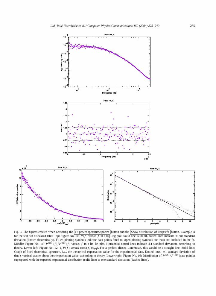
Figure No. 10: P(f ) versusf in a log–log plot. Blocked data points and the fitted function are shown.function represents the theoretical expectation value for the data points, and is shown with a full linshown, as two dotted lines, are±1 standard deviation of the Gaussiandistribution according to which thdata points scatter vertically about their expectation value.

Figure No. 11: P (ex)(f )/P (fit)(f ) versusf in a lin–lin plot (residual plot). For a perfect fit, this ratio scattabout the value 1 according to a Gaussian distribution. Two horizontal dotted lines denote±1 standard


fit.toline:f

Fig. 3. The figures created when activating theFit power spectrum/spectrabutton and theShow distribution of Pexp/Pfitbutton. Example isfor the test run discussed later. Top: Figure No. 10;P (f ) versusf in a log–log plot. Solid line is the fit, dotted lines indicate± one standarddeviation (known theoretically). Filled plotting symbols indicate datapoints fitted to, open plotting symbols are those not included in theMiddle: Figure No. 11;P (ex)(f )/P (fit)(f ) versusf in a lin–lin plot. Horizontal dotted lines indicate±1 standard deviation, accordingtheory. Lower left: Figure No. 12; 1/P (f ) versus cos(πf/fNyq). For a perfect aliased Lorentzian, this would be a straight line. SolidGraph of fitted theoretical spectrum, i.e., the theoretical expectation value for the experimental data. Dotted lines:±1 standard deviation odata’s vertical scatter about their expectation value, according to theory. Lower right: Figure No. 16; Distribution ofP (ex)/P (fit) (data points)superposed with the expected exponential distribution (solid line)± one standard deviation (dashed lines).


68%

eene data ine data

er spec-pushing

osed,

mandayed

ut. Thegorithm.e,ocedurear in thes

kingry. Thevalues

s

,

ideand was

deviation of this distribution. In this plot, the user may inspect the quality of the fit: For a perfect fit,� 2/3 of the data points fall within the two dotted lines and 1/3 outside.

Figure No. 12: 1/P (f ) versus cos(πf/fNyq). Blocked data points, fitted function, and±1 standard deviation arshown. For a power spectrum described by an aliased Lorentzian, the data fall on a straight line whplotted as here. As any deviance from a straight line is easily spotted by eye, so is the nature of ththis plot: It immediately reveals whether a Lorentzian fit is possible or not, and to which part of thit might be, if not in its entire frequency range.

Figure No. 13: Same as Figure No. 10, fory-coordinate.Figure No. 14: Same as Figure No. 11, fory-coordinate.Figure No. 15: Same as Figure No. 12, fory-coordinate.

Then, the user can choose to inspect the supposedly exponential distribution of the unblocked powtral values about their expectation value. This serves as yet another check of the data. WhenShow distribution of Pexp/Pfit, one (two) extra figures are produced:

Figure No. 16: Distribution ofP (ex)/P (fit), x-coordinate, using the unblocked experimental values. Superpthe expected exponential distribution (solid line)±1 standard deviation (dashed lines).

Figure No. 17: Same as Figure No. 16, fory-coordinate.

The resulting parameter values,χ2, and the support of the fit are given below the figure as well as in the comwindow of MatLab (MathWorks Inc.). Furthermore, the covariances between the fitted parameters are displboth places.

In general, the command window displays the progress of the various fits while they are carried odisplayed parameter values describe the progress of the fitting algorithm, the Levenberg–Marquardt alThe corresponding MatLab help menu (MathWorks Inc.) gives further information about definitions of step sizparameter “Lambda,” etc. Also, any error messages or warnings issued by the algorithm during the fitting prwill appear in the command window. Error messages due to input of improper parameter values will appecommand window in the format “Error message from program tweezercalib:. . .” together with error messagefrom MatLab caused by the error. The latter have the format “??? Error. . .”. All final results of fits appear in therelevant plot as well as in the command window.

4. Application

In the MatLab (MathWorks Inc.) command window, enter the commandfitsettings, thenstart_fit.Then proceed as follows:

(1) Click on the red buttonLoad time series. This opens a file-organizer that shows files in the current wordirectory of MatLab (MathWorks Inc.). Open the data file to be analyzed, change directory if necessainput window now displays more buttons and boxes to be filled in, as shown in Fig. 1. Default numericalare those applying to the test case.

(2) Choose value forfsample. If needed, redefine column numbersnx , ny , andnz. If nz = 0 the program doenot divideVx andVy by Vz, but uses them undivided asRx andRy , even if a third column withVz-values ispresent in the data file. Ifny = 0 the program only considers one coordinate (defined asx). In the test casefsample= 50 kHz,nx = 1, ny = 2, andnz = 3.

(3) If ny �= 0: Push the red buttonCheck for cross-talk, and inspect the resulting Figure No. 2 in order to decwhether or not to eliminate cross-talk between channels. The default action is to eliminate cross-talkapplied in the test case.


oweras

ringllows the

d lines

. Theer right

fortheerr is

ar that

ncies,low

Fig. 7

ee

ault: No

Stokes’metersfluid

al form,s.puter, with an:

e routines

(4) Click on the red buttonView data and wait while the data are processed: The program blocks the pspectra, and fits the two parameters,b andc, of the transformation that eliminates cross-talk if this option wchosen. Also, the program calculates histograms ofpositions, and it fits a Gaussian to each histogram. Duthis process, a number of windows are opened and the computer seems locked. Then, inspect as fofour to seven figures that pop up, each in its own window:

Figure No. 3: Check thatP (ex)xy /

√PxPy after elimination of cross-talk is equal to zero modulo error bars.

Figure No. 4 (5): Compare the histogram(s) with the Gaussian fit shown as a solid line with two dasheindicating±1 standard deviation of the scatter of bin-counts about the fitted Gaussian.χ2, the numberof degrees of freedomnfree, and the support of the Gaussian fit are all given below each figurenumber of bins in the histogram can be changed by entering a new number in the box in the uppcorner.

Figure No. 6 (7): Blocked power spectra. Inspect for drift/pointing instabilities at low frequencies: Lookexcess power at frequencies below∼ 50–100 Hz, depending on the quality of the data, wherepower spectrum should be constant iffc is larger than∼ 2–300 Hz. An example of excess powis seen for they-data in the lower left part of Fig. 2 for frequencies below 40 Hz. This powedue to beam pointing instability. Also, in the same frame, noise at 50 Hz lifts a data-point nefrequency.

Figure No. 8 (9): Inspect the power spectra for noise peaks at 50 Hz, 100 Hz, and at high frequeappearing as sharp peaks in power spectral values for distinct frequencies, and excess power atfrequencies. Noisy peaks and excess power from beam pointing instability are demonstrated inof [11].

(5) If needed, redefine values for number of data points in a block,nb, termination tolerance in fit, fitting rang(given byfmin andfmax) for the Lorentzian fit and for the final fit, and plotting range in final fit. Choose thfitting range of the final fit based on Figures No. 6–9 as described above. Test case:

nb = 350

termination tolerance= 10−3

Lorentzian fit fmin = 110 Hz fmax = 1000 Hz

Final fit fmin = 110 Hz fmax = 25 000 Hz

Plot fmin = 50 Hz fmax = 25 000 Hz

(6) Choose whether the position detection system should be treated as a virtual filter or not. If treated likefilter, choose which parameters should be fitted. Test case: Virtual filtering with two parameters. Defafiltering by position detection system.

(7) Decide whether the hydrodynamical drag force on the bead should be given by Stokes’ Law, or byfrequency-dependent result.Frequency dependent friction is used in test case. In that case, give paradescribing bead and fluid. In test case, bead diameter: 0.505 µm, height above surface: 11 µm, bead anddensities: 1 g/cm3, and kinematic viscosity: 1 µm2/s.

(8) If needed, redefine the number of electronic filters in the data acquisition pathway, and their functionif needed. Test case: Two first-order filters withf3dB = 50 kHz and 80 kHz, respectively. Default: No filter

(9) Click on Fit power spectrum/spectraand wait. Fitting may take some time (tens of minutes) and the comappears locked while fitting proceeds. For the test case, on a PC running MS Windows 2000 vs. 5.00Intel Pentium 4-processor, 2.00 GHz, 256MB RAM, fitting took about fifteen minutes.2 Results of test case

2 For users with long data files, faster F90 routines, based on NAGlib fitting packages, may be obtained from the authors. Thescome without a user-friendly graphics interface, though.


his

terval

terval

ge,

h-

nt

s-talk

each

x: y:

fc = 643± 14 Hz fc = 641± 14 HzD = (6.24± 0.09) · 102 (arb. units)2/s D = (6.48± 0.09) · 102 (arb. units)2/s

f(diode)3dB = 7.5± 0.1 kHz f

(diode)3dB = 7.1± 0.1 kHz

α(diode) = 0.26± 0.0 α(diode) = 0.26± 0.0χ2/nfree= 1.02 χ2/nfree= 0.96backing is 37% backing is 61%

(10) If wanted, click onShow distribution of Pexp/Pfitand wait.

Appendix A. List of program’s subroutines

fitsettings.m Sets path, sets defaults for a number of plotting variables. Most likely, the user should edit troutine, in particular change the path names to match the directories used by the user.

start_fit.m Main program. Creates input window.load_time_series.mSubroutine that loads the time series. Then calls:

input_para1.m Readsfsample, nx , ny , and creates theView data push-button. Ifny �= 0, it also createsthe Check for cross-talkpush-button. Calls:

input_para1_dec.m Reads whether elimination of cross-talk is chosen.check.m Checks that value entered corresponds to the allowed interval (upper end of in

included).check1.m Checks that value entered corresponds to the allowed interval (both ends of in

included).check2.m Checks that value entered is larger than zero.

input_para2.m Readsnb, reads fitting range for analytical Lorentzian fit, for final fit, for plotting ranand tolerance of fit. Also reads how the position detection system should be treated.

input_para3.m Reads whether frequency-dependent hydrodynamic friction is chosen. Creates the pusbuttons Fit power spectrum/spectraand Show distribution of Pexp/Pfit. Calls:

input_para3_hydro.m Reads the quantities needed for fitaccounting for frequency-dependehydrodynamic friction,R, ρbead, ρfluid, �, andν.

check_decorr.m Calculates and creates plot of cross-talk between channels.decorr_decision.m Sets relevant system variable depending on whether elimination of cros

between channels is wanted or not.min_corr.m Function to be minimized in order to eliminate cross-talk.

view_data.m Shows histogram(s) of position(s) and power spectrum (spectra) using:

plot_histogram.m Creates histogram plots.position_histogram_e.m Calculates position histogram and fits it with a Gaussian, integrated over

bin.caption.m Makes figure-captions.free_erf.m Gaussian function, integrated over bins, to fit to the position histogram.


lock,

ting

d

a virtual

ers are

more

a

c

E J.

5

s,

free_gauss.mGaussian function, used for display.calc_powersp.m Calculate the (yet not blocked) power spectrum of time series.plot_powerspectrum.m Creates log–log plots of blocked power spectra.plot_powerspec_lin.m Creates log–log plots of power spectra blocked with few data points per b

and blocked on the linear axis.

decorr_xy.m Performs the elimination of cross-talk between channels, i.e., calculatesP(ex)xy /

√P

(ex)x P

(ex)y

for transformed variables as function of transformation’s parameters, and chooses these by fit

P(ex)xy /

√P

(ex)x P

(ex)y to zero. Then plotsP (ex)

xy /

√P

(ex)x P

(ex)y before and after transformation an

P(ex)x andP

(ex)y after transformation.

plot_corrxy.m Creates plot ofP (ex)xy /

√P

(ex)x P

(ex)y .

diode_decision.m Sets a system variable depending on whether the position detection system acts asfilter, and whether one or two diode parameters are to be fitted when it does.

alias_decision.m Sets a system variable depending on whether aliasing should be accounted for or not.g_diode.m Characteristic function of virtual filter of diode. Depends on whether one or two diode paramet

chosen.hydro_decision.m Sets a system variable depending on whether frequency-dependenthydrodynamic friction is

used, or not.filter_decision.m Sets a system variable and filter function, depending on number of filters chosen.read_filter_function.m Reads user-defined filter function. Applies only when filters to be accounted for are

complicated than first-order filters.fit_powerspectrum.m Performs the fit using:

lorentz_analyt.m Estimates initial values for the parametersfc andD, based on analytic formulas forLorentzian function [1].

P_hydro.m The functional form of the power spectrum when frequency-dependent hydrodynamifriction is chosen.

P_theor.m The functional form of the power spectrum. Uses P_hydro.m when relevant.plot_fit.m Creates log–log plot of power spectrum versus frequency, along with the fit.plot_data_div_fit.m Creates lin–lin plot of data/fit versus frequency.plot_P_cos.m Creates lin–lin plot of 1/P (f ) versus cos(πf/fNyq).hist_decision.m Reads relevant system variable to determine if a histogram ofP (ex)/P (fit) should be

calculated and plotted.spectrum_histogram.m Calls the routine that plots distribution ofP (ex)/P (fit).plot_Phist.m Creates histogram of unblockedP (ex)/P (fit), and plots the normalized distribution.

References

[1] K. Berg-Sørensen, H. Flyvbjerg, Power spectrum analysis for optical tweezers, Rev. Sci. Instrum. 75 (3) (2004) 594–612.[2] K. Visscher, S.P. Gross, S.M. Block, Construction of multiple-beam optical traps with nanometer resolution position sensing, IEE

Select. Topics Quantum Electron. 2 (1996) 1066–1076.[3] K. Visscher, S.M. Block, Versatile optical traps with feedback control, Methods in Enzymology 298 (1998) 460–489.[4] K. Svoboda, C.F. Schmidt, B.J. Schnapp, S.M.Block, Direct observation of kinesin steppingby optical trapping interferometry, Nature 36

(1993) 721–727.[5] F. Gittes, C.F. Schmidt, Signals and noise in micromechanical measurements, Methods in Cell Biology 55 (1998) 129–156.[6] W.H. Press, B.P. Flannery, S.A. Teukolsky, W.T. Vetterling, Numerical Recipes. The Art of Scientific Computing, Cambridge Univ. Pres

Cambridge, 1986.


.optical

hical

al

ser

[7] L.P. Ghislain, N.A. Switz, W.W. Webb, Measurement of small forces using an optical trap, Rev. Sci. Instrum. 65 (1994) 2762–2768.[8] F. Gittes, C.F. Schmidt, Interference model for back-focal-plane displacement detection in optical tweezers, Opt. Lett. 23 (1998) 7–9[9] A. Pralle, M. Prummer, E.-L. Florin, E.H.K. Stelzer, J.K.H. Hörber, Three-dimensional high-resolution particle tracking for

tweezers by forward scattered light, Microscopy Research and Technique 44 (1999) 378–386.[10] G.G. Stokes, On the effect of the internal friction of fluids onthe motion of pendulums, Transactions of the Cambridge Philosop

Society IX (1851) 8–106.[11] H. Flyvbjerg, unpublished, 2003.[12] K. Berg-Sørensen, L. Oddershede, E.-L.Florin, H. Flyvbjerg, Unintended filtering ina typical photodiode detection system for optic

tweezers, J. Appl. Phys. 93 (2003) 3167–3176.[13] K. Berg-Sørensen, E.G.J. Peterman, M. van Dijk, C. Schmidt, H. Flyvbjerg, Power spectrum analysis for optical tweezers, II: La

wavelength dependence of unintended filtering and how to achieve high band-width with precision, 2004, submitted for publication.[14] N.C. Barford, Experimental Measurements: Precision, Error and Truth, second ed., Wiley, New York, 1986.[15] MathWorks Inc., MatLab Help Menu, Optional parameters of lsqnonlin, Optimization toolbox.

matlab program for precision calibration of optical tweezers program for... · computer physics...

Documents