MATLAB PrimerThird Edition

Editor : Kermit Sigmon

Department of Mathematics, University of Florida

Re-editor : Byeong-Chun Shin

Department of Mathematics, Chonnam National University

Copyright c⃝1989, 1992, 1993 by Kermit Sigmon

Introduction

MATLAB is an interactive, matrix-based system for scientific and engineering numeric computation

and visualization. You can solve complex numerical problems in a fraction of the time required with a

programming language such as Fortran or C. The name MATLAB is derived from MATrix LABoratory.

The purpose of this Primer is to help you begin to use MATLAB. It is not intended to be a substitute

for the User’s Guide and Reference Guide for MATLAB. The Primer can best be used hands-on. You

are encouraged to work at the computer as you read the Primer and freely experiment with examples.

This Primer, along with the on-line help facility, usually suffice for students in a class requiring use of

MATLAB.

You should liberally use the on-line help facility for more detailed information. When using MATLAB,

the command help functionname will give information about a specific function. For example, the

command help eig will give information about the eigenvalue function eig. By itself, the command help

will display a list of topics for which on-line help is available; then help topic will list those specific

functions under this topic for which help is available. The list of functions in the last section of this

Primer also gives most of this information. You can preview some of the features of MATLAB by first

entering the command demo and then selecting from the options offered.

The scope and power of MATLAB go far beyond these notes. Eventually you will want to consult the

MATLAB User’s Guide and Reference Guide. Copies of the complete documentation are often available

i

for review at locations such as consulting desks, terminal rooms, computing labs, and the reserve desk of

the library. Consult your instructor or your local computing center to learn where this documentation is

located at your institution.

MATLAB is available for a number of environments:

Sun/Apollo/VAXstation/HP workstations, VAX, MicroVAX, Gould, PC and AT compatibles, 80386

and 80486 computers, Apple Macintosh, and several parallel machines. There is a relatively inexpensive

Student Edition available from Prentice Hall publishers. The information in these notes applies generally

to all of these environments.

MATLAB is licensed by The MathWorks, Inc., 24 Prime Park Way, Natick, MA 01760, (508)653-

1415, Fax: (508)653-2997, Email: info@mathworks.com.

Copyright c⃝1989, 1992, 1993 by Kermit Sigmon

ii

Contents

Page

1. Accessing MATLAB . . . . . . . . . . . . . . . . . . . . . . . . . . . . . . . . . . . . . . . . . . . . . . . . . . . . . . . . . . . . . 1

2. Entering matrices . . . . . . . . . . . . . . . . . . . . . . . . . . . . . . . . . . . . . . . . . . . . . . . . . . . . . . . . . . . . . . . 1

3. Matrix operations, array operations . . . . . . . . . . . . . . . . . . . . . . . . . . . . . . . . . . . . . . . . . . . . . . . . . 2

4. Statements, expressions, variables; saving a session . . . . . . . . . . . . . . . . . . . . . . . . . . . . . . . . . . . . . 3

5. Matrix building functions . . . . . . . . . . . . . . . . . . . . . . . . . . . . . . . . . . . . . . . . . . . . . . . . . . . . . . . . . 4

6. For, while, if — and relations . . . . . . . . . . . . . . . . . . . . . . . . . . . . . . . . . . . . . . . . . . . . . . . . . . . . . . 4

7. Scalar functions . . . . . . . . . . . . . . . . . . . . . . . . . . . . . . . . . . . . . . . . . . . . . . . . . . . . . . . . . . . . . . . . . 7

8. Vector functions . . . . . . . . . . . . . . . . . . . . . . . . . . . . . . . . . . . . . . . . . . . . . . . . . . . . . . . . . . . . . . . . 7

9. Matrix functions . . . . . . . . . . . . . . . . . . . . . . . . . . . . . . . . . . . . . . . . . . . . . . . . . . . . . . . . . . . . . . . . 7

iii

10. Command line editing and recall . . . . . . . . . . . . . . . . . . . . . . . . . . . . . . . . . . . . . . . . . . . . . . . . . . . 8

11. Submatrices and colon notation . . . . . . . . . . . . . . . . . . . . . . . . . . . . . . . . . . . . . . . . . . . . . . . . . . . . 8

12. M-files: script files, function files . . . . . . . . . . . . . . . . . . . . . . . . . . . . . . . . . . . . . . . . . . . . . . . . . . . 9

13. Text strings, error messages, input . . . . . . . . . . . . . . . . . . . . . . . . . . . . . . . . . . . . . . . . . . . . . . . . . 12

14. Managing M-files . . . . . . . . . . . . . . . . . . . . . . . . . . . . . . . . . . . . . . . . . . . . . . . . . . . . . . . . . . . . . . . 13

15. Comparing efficiency of algorithms: flops, tic, toc . . . . . . . . . . . . . . . . . . . . . . . . . . . . . . . . . . . . . 14

16. Output format . . . . . . . . . . . . . . . . . . . . . . . . . . . . . . . . . . . . . . . . . . . . . . . . . . . . . . . . . . . . . . . . . 14

17. Hard copy . . . . . . . . . . . . . . . . . . . . . . . . . . . . . . . . . . . . . . . . . . . . . . . . . . . . . . . . . . . . . . . . . . . . 15

18. Graphics . . . . . . . . . . . . . . . . . . . . . . . . . . . . . . . . . . . . . . . . . . . . . . . . . . . . . . . . . . . . . . . . . . . . . 15

planar plots (15), hardcopy (17), 3-D line plots (18)

mesh and surface plots (18), Handle Graphics (20)

19. Sparse matrix computations . . . . . . . . . . . . . . . . . . . . . . . . . . . . . . . . . . . . . . . . . . . . . . . . . . . . . . 20

20. Reference . . . . . . . . . . . . . . . . . . . . . . . . . . . . . . . . . . . . . . . . . . . . . . . . . . . . . . . . . . . . . . . . . . . . . 22

iv

1. Accessing MATLAB.

• Starting MATLAB with the system command : matlab

• In linux system, starting MATLAB with the system command : matlab -nojvm

• Exiting MATLAB with the MATLAB command : quit or exit.

• help plot

• up/down arrow

2. Entering matrices.

Matrices can be introduced into MATLAB in several different ways:

• Entered by an explicit list of elements,

• Generated by built-in statements and functions,

• Created in a diskfile with your local editor,

• Loaded from external data files or applications (see the User’s Guide).

1

For example, either of the statements

A = [1 2 3; 4 5 6; 7 8 9]

and

A = [

1 2 3

4 5 6

7 8 9 ]

creates the obvious 3-by-3 matrix and assigns it to a variable A.

• The elements within a row of a matrix may be separated by commas as well as a blank.

• When listing a number in exponential form (e.g. 2.34e-9), blank spaces must be avoided.

• MATLAB allows complex numbers in all its operations and functions.

2

Individual matrix and vector entries can be referenced with indices inside parentheses in the

usual manner.

• For example, A(2, 3) denotes the entry in the second row, third column of matrix A and

• x(3) denotes the third coordinate of vector x.

• A matrix or a vector will only accept positive integers as indices.

• rand(n) : create an n×n matrix with randomly generated entries distributed uniformly

between 0 and 1,

• while rand(m,n) will create an m× n one.

3

3. Matrix operations, array operations.

The following matrix operations are available in MATLAB:

+ addition

− subtraction

∗ multiplication

power

′ conjugate transpose

\ left division

/ right division

• These matrix operations apply, of course, to scalars (1-by-1 matrices) as well.

• If the sizes of the matrices are incompatible for the matrix operation, an error message

will result, except in the case of scalar-matrix operations.

4

The “matrix division” operations deserve special comment.

• If A is an invertible square matrix and

• b is a compatible column, resp. row, vector, then

x = A\b is the solution of A ∗ x = b and, resp.,

x = b/A is the solution of x ∗A = b.

In left division,

• if A is square, then it is factored using Gaussian elimination and these factors are used

to solve A ∗ x = b.

• If A is not square, it is factored using Householder orthogonalization with column pivot-

ing and the factors are used to solve the under- or over- determined system in the least

squares sense.

Right division is defined in terms of left division by b/A = (A′\b′)′.

5

Array operations.

• The matrix operations of addition and subtraction already operate entry-wise but,

• the other matrix operations given above do not—they are matrix operations.

• It is important to observe that these other operations, ∗, , \, and /, can be made to

operate entry-wise by preceding them by a period.

• e.g., either [1,2,3,4].*[1,2,3,4] or [1,2,3,4]. 2 will yield [1,4,9,16].

• This is particularly useful when using Matlab graphics.

6

4. Statements, expressions, and variables; saving a session.

MATLAB is an expression language; the expressions you type are interpreted and evaluated.

MATLAB statements are usually of the form

variable = expression, or simply

expression

• Expressions are usually composed from operators, functions, and variable names.

• Evaluation of the expression produces a matrix, which is then displayed on the screen

and assigned to the variable for future use.

• If the variable name and = sign are omitted, a variable ans (for answer) is automatically

created to which the result is assigned.

• A statement is normally terminated with the carriage return.

• However, a statement can be continued to the next line with three periods(...) followed

by a carriage return.

7

• On the other hand, several statements can be placed on a single line if separated by

commas(,) or semicolons(;).

• If the last character of a statement is a semicolon, the printing is suppressed, but the

assignment is carried out.

• This is essential in suppressing unwanted printing of intermediate results.

• MATLAB is case-sensitive in the names of commands, functions, and variables. For

example, solveUT is not the same as solveut.

• The command who (or whos) will list the variables currently in the workspace.

• A variable can be cleared from the workspace with the command clear variablename.

+ The command clear alone will clear all nonpermanent variables.

• The permanent variable eps (epsilon) gives the machine unit roundoff—about 10−16 on

most machines. It is useful in specifying tolerences for convergence of iterative processes.

• A runaway computation can be stopped with CTRL-C(CTRL-BREAK on PC).

8

Saving a session.

• When one logs out or exits MATLAB all variables are lost.

• However, invoking the command save before exiting causes all variables to be written to

a non-human-readable diskfile named matlab.mat.

• The command save fname X Y saves to fname.mat X Y only as variables.

• When one later reenters MATLAB, the command load will restore the workspace to its

former state.

9

5. Matrix building functions.

Convenient matrix building functions are

eye identity matrix

zeros matrix of zeros

ones matrix of ones

diag create or extract diagonals

triu upper triangular part of a matrix

tril lower triangular part of a matrix

rand randomly generated matrix

hilb Hilbert matrix

magic magic square

toeplitz see help toeplitz

10

• For example, zeros(m,n) produces an m-by-n matrix of zeros and zeros(n) produces an

n-by-n one.

• If A is a matrix, then zeros(size(A)) produces a matrix of zeros having the same size as

A.

• If x is a vector, diag(x) is the diagonal matrix with x down the diagonal.

• If A is a square matrix, then diag(A) is a vector consisting of the diagonal of A.

• What is diag(diag(A))? Try it.

• Matrices can be built from blocks. For example, if A is a 3-by-3 matrix, then

B = [A, zeros(3,2); zeros(2,3), eye(2)]

11

6. For, while, if — and relations.

In their basic forms, these MATLAB flow control statements operate like those in most

computer languages.

For.

For example, for a given n, the statement

x = []; for i = 1:n, x=[x,i 2], endor

x = [];

for i = 1:n

x = [x,i 2]end

will produce a certain n-vector and the statement

x = []; for i = n:-1:1, x=[x,i 2], end12

The statements

for i = 1:m

for j = 1:n

H(i, j) = 1/(i+j-1);

end

end

H

will produce and print to the screen the m-by-n hilbert matrix.

• The semicolon on the inner statement is essential to suppress printing of unwanted

intermediate results while the last H displays the final result.

13

• The for statement permits any matrix to be used instead of 1:n.

• The variable just consecutively assumes the value of each column of the matrix.

For example,

s = 0;

for c = A

s = s + sum(c);

end

computes the sum of all entries of the matrix A by adding its column sums.

+ (Of course, sum(sum(A)) does it more efficiently; see section 8).

+ In fact, since 1:n = [1,2,3,. . . ,n], this column-by-column assigment is what occurs

with “if i = 1:n,. . . ” (see section 11).

14

While.

The general form of a while loop is

while relation

statements

end

• The statements will be repeatedly executed as long as the relation remains true.

• For example, for a given number a, the following will compute and display the smallest

nonnegative integer n such that 2n ≥ a:

n = 0;

while 2 n < a

n = n + 1;

end

n

15

If.

if relation

statements

end

• The statements will be executed only if the relation is true.

• Multiple branching is also possible, as is illustrated by

if n < 0

parity = 0;

elseif rem(n,2) == 0

parity = 2;

else

parity = 1;

end

16

Relations.

The relational operators in MATLAB are

< less than

> greater than

<= less than or equal

>= greater than or equal

== equal

∼= not equal.

• Note that “=” is used in an assignment statement while “==” is used in a relation.

• Relations may be connected or quantified by the logical operators

& and

| or

∼ not.

17

• When applied to scalars, a relation is actually the scalar 1 or 0 depending on whether

the relation is true or false.

+ Try entering 3 < 5, 3 > 5, 3 == 5, and 3 == 3.

• When applied to matrices of the same size, a relation is a matrix of 0’s and 1’s giving

the value of the relation between corresponding entries.

+ Try a = rand(5), b = triu(a), a == b.

• A relation between matrices is interpreted by while and if to be true if each entry of the

relation matrix is nonzero.

• Hence, if you wish to execute statement when matrices A and B are equal you could

type

if A == B

statement

end

18

• but if you wish to execute statement when A and B are not equal, you would type

if any(any(A ∼= B))

statement

end

or, more simply,

if A == B else

statement

end

Note that the seemingly obvious

if A ∼= B, statement, end

statement would execute only if each of the corresponding entries of A and B differ.

• The function any returns “True(1)” if any element of a vector is nonzero.

• The function all “True(1)” if all elements of a vector are nonzero.

19

7. Scalar functions.

• Certain MATLAB functions operate essentially on scalars,

• but operate element-wise when applied to a matrix.

• The most common such functions are

sin asin exp abs round

cos acos log (natural log) sqrt floor

tan atan rem (remainder) sign ceil

20

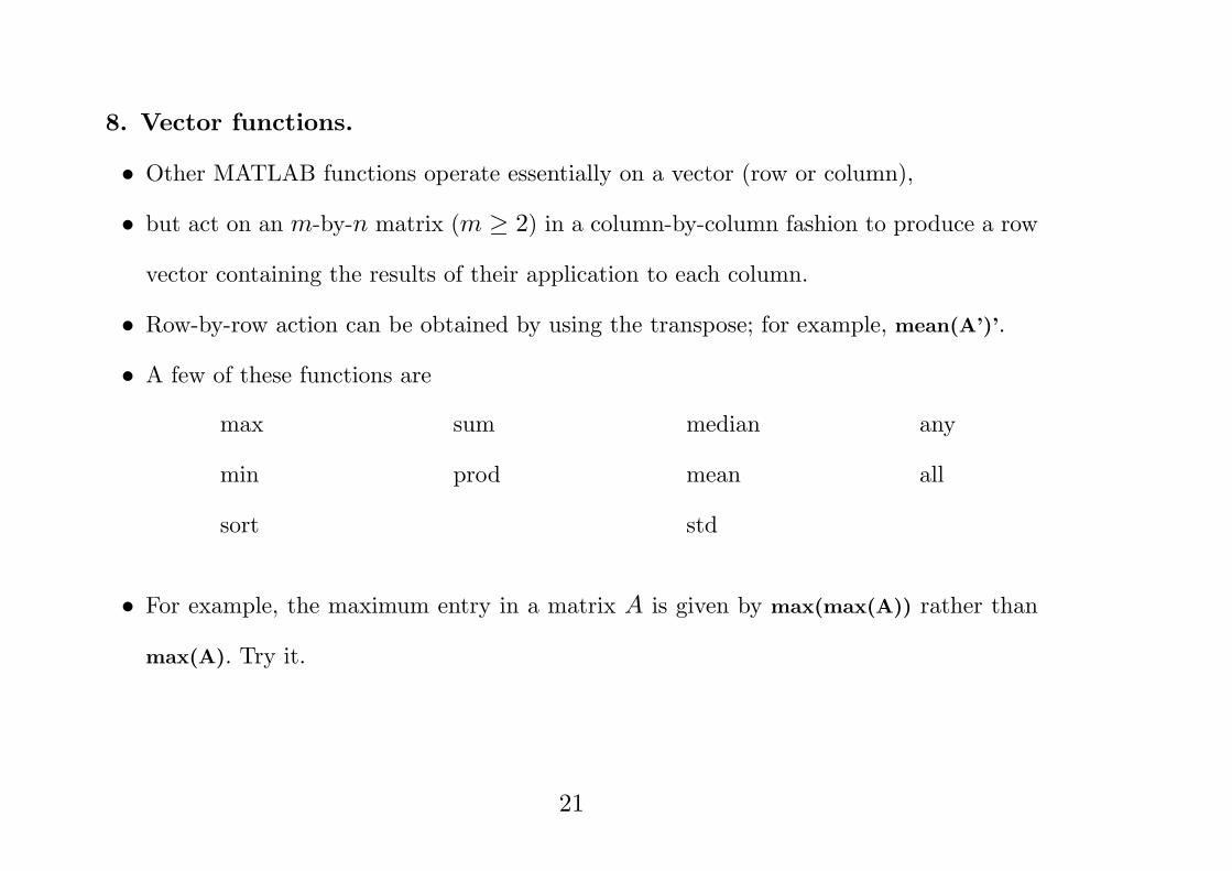
8. Vector functions.

• Other MATLAB functions operate essentially on a vector (row or column),

• but act on an m-by-n matrix (m ≥ 2) in a column-by-column fashion to produce a row

vector containing the results of their application to each column.

• Row-by-row action can be obtained by using the transpose; for example, mean(A’)’.

• A few of these functions are

max sum median any

min prod mean all

sort std

• For example, the maximum entry in a matrix A is given by max(max(A)) rather than

max(A). Try it.

21

9. Matrix functions.

Much of MATLAB’s power comes from its matrix functions.

eig eigenvalues and eigenvectors

inv inverse

poly characteristic polynomial

det determinant

size size

cond condition number in the 2-norm

rank rank

norm 1-norm, 2-norm, F-norm, ∞-norm

expm matrix exponential

sqrtm matrix square root

22

rref reduced row echelon form

lu LU factorization

qr QR factorization

chol cholesky factorization

svd singular value decomposition

hess hessenberg form

schur schur decomposition

MATLAB functions may have single or multiple output arguments. For example,

y = eig(A), or simply eig(A)

produces a column vector containing the eigenvalues of A while

[U,D] = eig(A)

• produces a matrix U whose columns are the eigenvectors of A and

• a diagonal matrix D with the eigenvalues of A on its diagonal. Try it.

23

10. Command line editing and recall.

• The command line in MATLAB can be easily edited.

• The cursor can be positioned with the left/right arrows and the Backspace (or Delete)

key used to delete the character to the left of the cursor.

• A convenient feature is use of the up/down arrows to scroll through the stack of previous

commands.

• One can, therefore, recall a previous command line, edit it, and execute the revised

command line.

• For small routines, this is much more convenient that using an M-file which requires

moving between MATLAB and the editor (see sections 12 and 14).

24

11. Submatrices and colon notation.

• Vectors and submatrices are often used in MATLAB to achieve fairly complex data

manipulation effects.

• Colon notation” (which is used both to generate vectors and reference submatrices) and

subscripting by integral vectors are keys to efficient manipulation of these objects.

• Creative use of these features to vectorize operations permits one to minimize the use of

loops (which slows MATLAB) and to make code simple and readable.

• Special effort should be made to become familiar with them.

• The expression 1:5 (met earlier in for statements) is actually the row vector [1 2 3 4 5].

• The numbers need not be integers nor the increment one.

• For example, 0.2:0.2:1.2 gives [0.2, 0.4, 0.6, 0.8, 1.0, 1.2],

and 5:-1:1 gives [5 4 3 2 1].

25

• The following statements will, for example, generate a table of sines.

x = [0.0:0.1:2.0]′; y = sin(x); [x y]

• Note that since sin operates entry-wise, it produces a vector y from the vector x.

• The colon notation can be used to access submatrices of a matrix. For example,

A(1:4,3) is the column vector consisting of the first four entries of the third column.

• A colon by itself denotes an entire row or column:

A(:,3) is the third column of A, and A(1:4,:) is the first four rows.

• Arbitrary integral vectors can be used as subscripts:

A(:,[2 4]) contains as columns, columns 2 and 4 of A.

• Such subscripting can be used on both sides of an assignment statement:

A(:,[2 4 5]) = B(:,1:3) replaces columns 2,4,5 of A with the first three columns of

B. Note that the entire altered matrix A is printed and assigned.

26

• Columns 2 and 4 of A can be multiplied on the right by the 2-by-2 matrix [1 2;3 4]:

A(:,[2,4]) = A(:,[2,4])*[1 2;3 4]

Once again, the entire altered matrix is printed and assigned.

• If x is an n-vector, what is the effect of the statement x = x(n:-1:1)? Try it.

Also try y = fliplr(x) and y = flipud(x’) : flip left/right and up/down.

27

12. M-files.

• MATLAB can execute a sequence of statements stored in diskfiles.

• Such files are called “M-files” because they must have the file type of “.m” as the exten-

sion.

• Much of your work with MATLAB will be in creating and refining M-files.

• M-files are usually created using your local editor.

• There are two types of M-files: script files and function files.

Script files.

• A script file consists of a sequence of normal MATLAB statements.

• If the file has the filename, say, rotate.m, then the MATLAB command rotate will cause

the statements in the file to be executed.

28

• Variables in a script file are global and will change the value of variables of the same

name in the environment of the current MATLAB session.

• Script files may be used to enter data into a large matrix; in such a file, entry errors can

be easily corrected.

• If, for example, one enters in a diskfile data.m

A = [

1 2 3 4

5 6 7 8

];

then the MATLAB statement data will cause the assignment given in data.m

to be carried out.

• However, it is usually easier to use the MATLAB function load (see section 2).

• An M-file can reference other M-files, including referencing itself recursively.

29

Function files.

• Function files provide extensibility to MATLAB.

• You can create new functions specific to your problem which will then have the same

status as other MATLAB functions.

• Variables in a function file are by default local.

• A variable can, however, be declared global (see help global).

• We first illustrate with a simple example of a function file.

function a = randint(m,n)

%RANDINT Randomly generated integral matrix.

% randint(m,n) returns an m-by-n such matrix with entries

% between 0 and 9.

a = floor(10*rand(m,n));

30

function a = randint(m,n,a,b)

%RANDINT Randomly generated integral matrix.

% randint(m,n) returns an m-by-n such matrix with entries

% between 0 and 9.

% rand(m,n,a,b) return entries between integers a and b.

if nargin < 3, a = 0; b = 9; end

a = floor((b−a+1)*rand(m,n)) + a;

• This should be placed in a diskfile with filename randint.m.

• The first line declares the function name, input arguments, and output arguments; with-

out this line the file would be a script file.

• Note that use of nargin (“number of input arguments”) permits one to set a default

value of an omitted input variable—such as a and b in the example.

• The % symbol indicates that the rest of the line is a comment; ignore the rest of it.

31

• A function may also have multiple output arguments. For example:

function [mean, stdev] = stat(x)

% STAT Mean and standard deviation

% For a vector x, stat(x) returns the mean of x;

% [mean, stdev] = stat(x) both the mean and standard deviation.

% For a matrix x, stat(x) acts columnwise.

[m n] = size(x);

if m == 1

m = n; % handle case of a row vector

end

mean = sum(x)/m;

stdev = sqrt(sum(x. 2)/m - mean. 2);

32

• Once this is placed in a diskfile stat.m, a MATLAB command [xm, xd] = stat(x), for

example, will assign the mean and standard deviation of the entries in the vector x to

xm and xd, respectively.

• Single assignments can also be made with a function having multiple output arguments.

• For example, xm = stat(x) (no brackets needed around xm) will assign the mean of x

to xm.

• Moreover, the first few contiguous comment lines, which document the M-file, are avail-

able to the on-line help facility and will be displayed if, for example, help stat is entered.

• Such documentation should always be included in a function file.

• This function illustrates some of the MATLAB features that can be used to produce

efficient code.

• Note, for example, that X. 2 is the matrix of squares of the entries of X , that sum

is a vector function (section 8), that sqrt is a scalar function (section 7), and that the

33

division in sum(x)/m is a matrix-scalar operation.

• Thus all operations are vectorized and loops avoided.

If you can’t vectorize some computations,

• you can make your for loops go faster by preallocating any vectors or matrices in which

output is stored.

• For example, by including “E=zeros(6,50)” of the first statement below, which uses the

function zeros, space for storing E in memory is preallocated.

• Without this MATLAB must resize E one column larger in each iteration, slowing

execution.

M = magic(6); E = zeros(6,50);

for j = 1:50

E(:,j) = eig(M i);

end

34

Some more advanced features are illustrated by the following function.

• nargin : “number of input arguments”

• nargout : “number of output arguments”

• feval permits one to have as an input variable a string naming another function.

function [A, B] = main(fun, x, y)

% Initialization

if nargin < 2, y = 1; end

if (x > y), A = feval(fun, x); B = feval(fun, y);

else

A = feval(fun, y); B = feval(fun, x);

end

end

• Some of MATLAB’s functions are built-in while others are distributed as M-files.

35

• The actual listing of any non-built-in M-file—MATLAB’s or your own—can be viewed

with the MATLAB command type functionname.

13. Text strings, error messages, input.

• Text strings are entered into MATLAB surrounded by single quotes. For example, s =

’This is a test’ assigns the given text string to the variable s.

• Text strings can be displayed with the function disp. For example:

disp(’this message is hereby displayed’)

• Error messages are best displayed with the function error

error(’Sorry, the matrix must be symmetric’)

since when placed in an M-File, it aborts execution of the M-file.

• In an M-file the user can be prompted to interactively enter input data with the function

input. When, for example, the statement

36

iter = input(’Enter the number of iterations: ’)

is encountered, the prompt message is displayed and execution pauses. Upon pressing

the return key, the data is assigned to the variable iter and execution resumes.

14. Managing M-files.

• edit

• !command

• help dbtype, help dbtype myfilename

• pwd

• cd, dir, ls, what

• who whos

• delete, type

• help path.

37

15. Comparing efficiency of algorithms: tic, toc, etime, cputime.

The elapsed time (in seconds) can be obtained with the stopwatch timers tic and toc;

• tic starts the timer and toc returns the elapsed time. Hence, the commands

tic, any statement, toc

will return the elapsed time for execution of the statement. For example

tic, x = A\b; toc

t=cputime; x = A\b; cputime-t

• It should be noted that, on timesharing machines, elapsed time may not be a reliable

measure of the efficiency of an algorithm since the rate of execution depends on how

busy the computer is at the time.

38

16. Output format.

• While all computations in MATLAB are performed in double precision,

• the format of the displayed output can be controlled by the following commands.

format short fixed point with 4 decimal places (the default)

format long fixed point with 14 decimal places

format short e scientific notation with 4 decimal places

format long e scientific notation with 15 decimal places

format rat approximation by ratio of small integers

format hex hexadecimal format

format bank fixed dollars and cents

format + +, -, blank

Once invoked, the chosen format remains in effect until changed.

39

17. Hardcopy.

• Hardcopy is most easily obtained with the diary command.

• The command diary filename causes what appears subsequently on the screen (except

graphics) to be written to the named diskfile

if the filename is omitted it will be written to a default file named diary until one gives

the command diary off; the command diary on will cause writing to the file to resume.

When finished, you can edit the file as desired and print it out on the local system.

40

18. Graphics.

MATLAB can produce planar plots of curves, 3-D plots of curves, 3-D mesh surface plots,

and 3-D faceted surface plots.

• The primary commands for these facilities are

plot, plot3, mesh, and surf, respectively.

• To preview some of these capabilities, enter the command demo and select some of the

graphics options.

41

Planar plots.

• The plot command creates linear x-y plots;

if x and y are vectors of the same length, the command plot(x,y) opens a graphics

window and draws an x-y plot of the elements of x versus the elements of y.

• For example,

x = -4:.01:4; y = sin(x); plot(x,y)

• The vector x is a partition of the domain with meshsize 0.01 while y is a vector giving

the values of sine at the nodes of this partition.

• figure(n)

• MATLAB supplies a function fplot to easily and efficiently plot the graph of a function.

fplot(’sin’, [-pi,pi])

• Plots of parametrically defined curves can also be made.

t=0:.001:2*pi; x=cos(3*t); y=sin(2*t); plot(x,y)

42

• The graphs can be given titles, axes labeled, and text placed within the graph with the

following commands which take a string as an argument.title graph title

xlabel x-axis label

ylabel y-axis label

gtext place text on the graph using the mouse

text position text at specified coordinates

• For example, the command

title(’Best Least Squares Fit’)

gtext(’The Spot’)

help text

grid

43

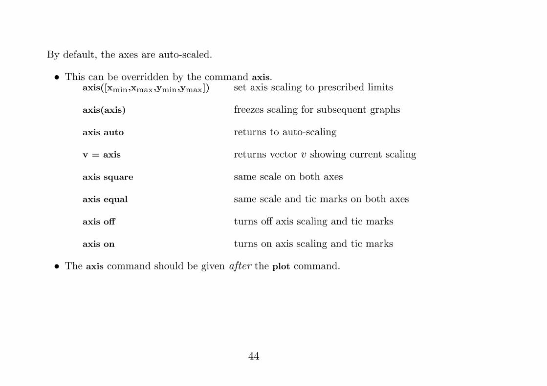
By default, the axes are auto-scaled.

• This can be overridden by the command axis.axis([xmin,xmax,ymin,ymax]) set axis scaling to prescribed limits

axis(axis) freezes scaling for subsequent graphs

axis auto returns to auto-scaling

v = axis returns vector v showing current scaling

axis square same scale on both axes

axis equal same scale and tic marks on both axes

axis off turns off axis scaling and tic marks

axis on turns on axis scaling and tic marks

• The axis command should be given after the plot command.

44

• Two ways to make multiple plots on a single graph are illustrated by

x=0:.01:2*pi;y1=sin(x);y2=sin(2*x);y3=sin(4*x);plot(x,y1,x,y2,x,y3)

• and by forming a matrix Y containing the functional values as columns

x=0:.01:2*pi; Y=[sin(x)’, sin(2*x)’, sin(4*x)’]; plot(x,Y)

• Another way is with hold.

+ hold on hold off

One can override the default linetypes, pointtypes and colors. For example,

x=0:.01:2*pi; y1=sin(x); y2=sin(2*x); y3=sin(4*x);

plot(x,y1,’–’,x,y2,’:’,x,y3,’+’)

renders a dashed line and dotted line for the first two graphs while for the third the

symbol + is placed at each node.

45

• The line- and mark-types are

Linetypes: solid (-), dashed (–). dotted (:), dashdot (-.)

Marktypes: point (.), plus (+), star (*), circle (o), x-mark (x)

• Colors can be specified for the line- and mark-types.

Colors: yellow (y), magenta (m), cyan (c), red (r)

green (g), blue (b), white (w), black (k)

• For example, plot(x,y,’r–’) plots a red dashed line.

• The command subplot can be used to partition the screen so that several small plots

can be placed in one figure. See help subplot.

• Other specialized 2-D plotting functions you may wish to explore via help are:

polar, bar, hist, quiver, compass, feather, rose, stairs, fill

46

Graphics hardcopy

• A hardcopy of the current graphics figure can be most easily obtained with the MATLAB

command print.

• Entered by itself, it will send a high-resolution copy of the current graphics figure to the

default printer.

• The printopt M-file is used to specify the default setting used by the print command. If

desired, one can change the defaults by editing this file (see help printopt).

• The command print filename saves the current graphics figure to the designated

filename in the default file format.

• If, for example, PostScript is the default file format, then

print lissajous

will create a PostScript file lissajous.ps of the current graphics figure which can subse-

quently be printed using the system print command.

47

• If filename already exists, it will be overwritten unless you use the -append option.

• The command print -append lissajous will append the (hopefully different) current

graphics figure to the existing file lissajous.ps.

• In this way one can save several graphics figures in a single file.

• The default settings can, of course, be overwritten. For example,

print -deps -f3 saddle

will save to an Encapsulated PostScript file saddle.eps the graphics figure 3 — even if it

is not the current figure.

48

3-D line plots.

• The command plot3 produces curves in three dimensional space.

• If x, y, and z are three vectors of the same size, then the command plot3(x,y,z) will

produce a perspective plot of the piecewise linear curve in 3-space passing through the

points whose coordinates are the respective elements of x, y, and z.

• These vectors are usually defined parametrically. For example,

t=.01:.01:20*pi; x=cos(t); y=sin(t); z=t. 3; plot3(x,y,z)

will produce a helix which is compressed near the x-y plane (a “slinky”). Try it.

• Just as for planar plots, a title and axis labels (including zlabel) can be added.

• The features of axis command described there also hold for 3-D plots;

setting the axis scaling to prescribed limits will, of course, now require a 6-vector.

49

3-D mesh and surface plots.

• Three dimensional wire mesh surface plots are drawn with the command mesh.

• The command mesh(z) creates a three-dimensional perspective plot of the elements of

the matrix z.

• The mesh surface is defined by the z-coordinates of points above a rectangular grid in

the x-y plane. Try mesh(eye(10)).

• The command surf : three dimensional faceted surface plots. Try surf(eye(10)).

• To draw the graph of a function z = f(x, y) over a rectangle,

one first defines vectors xx and yy which give partitions of the sides of the rectangle.

• With the function meshgrid one then creates a matrix x, each row of which equals xx

and whose column length is the length of yy, and similarly a matrix y, each column of

which equals yy, as follows:

[x,y] = meshgrid(xx,yy);

50

• One then computes a matrix z, obtained by evaluating f entrywise over the matrices x

and y, to which mesh or surf can be applied.

• You can, for example, draw the graph of z = e−x2−y2

over the square [−2, 2]× [−2, 2]

as follows (try it):

xx = -2:.2:2; yy = xx;

[x,y] = meshgrid(xx,yy);

z = exp(-x. 2 - y. 2);

mesh(z), or surf(z)

One could, of course, replace the first three lines of the preceding with

[x,y] = meshgrid(-2:.2:2, -2:.2:2);

• The color shading of surfaces is set by the shading command.

There are three settings for shading: faceted (default), interpolated, and flat.

shading faceted, shading interp, or shading flat

51

• The color profile of a surface is controlled by the colormap command.

Available predefined colormaps include:

hsv (default), hot, cool, jet, pink, copper, flag, gray, bone

• The command colormap(cool) will, for example, set a certain color profile for the current

figure. Experiment with various colormaps on the surface produced above.

• The command view can be used to specify in spherical or cartesian coordinates the

viewpoint from which the 3-D object is to be viewed. See help view.

• The MATLAB function peaks generates an interesting surface on which to experiment

with shading, colormap, and view.

• The MATLAB functions sphere and cylinder will generate such plots of the named

surfaces. (See type sphere and type cylinder.)

• Other 3-D plotting functions you may wish to explore via help are:

meshz, surfc, surfl, contour, pcolor

52

19. Sparse Matrix Computations.

In performing matrix computations, MATLAB normally assumes that a matrix is dense;

that is, any entry in a matrix may be nonzero.

• If, however, a matrix contains sufficiently many zero entries,

computation time could be reduced by avoiding arithmetic operations on zero entries,

less memory could be required by storing only the nonzero entries of the matrix.

• This increase in efficiency in time and storage can make feasible the solution of signifi-

cantly larger problems than would otherwise be possible.

• MATLAB provides the capability to take advantage of the sparsity of matrices.

Matlab has two storage modes, full and sparse, with full the default.

• The functions full and sparse convert between the two modes.

• For a matrix A, full or sparse, nnz(A) returns the number of nonzero elements in A.

• A sparse matrix is stored as a linear array of its nonzero elements along with their row

53

and column indices.

• If a full tridiagonal matrix F is created via, say,

F = floor(10*rand(6)); F = triu(tril(F,1),-1);

then the statement S = sparse(F) will convert F to sparse mode.

• The statement F = full(S) restores S to full storage mode.

• One can check the storage mode of a matrix A with the command issparse(A).

• A sparse banded matrix can be easily created via the function spdiags by specifying

diagonals. For example, a familiar sparse tridiagonal matrix is created by

m = 6; n = 6; e = ones(n,1); d = -2*e;

T = spdiags([e,d,e],[-1,0,1],m,n)

• The integral vector [-1,0,1] specifies in which diagonals the columns of [e,d,e] should be

placed (use full(T) to view).

• See help spdiags for further features of spdiags.

54

The sparse analogs of eye, zeros, ones, and randn for full matrices are, respectively,

speye, sparse, spones, sprandn

• The command sparse(m,n) creates a sparse zero matrix.

The versatile function sparse permits creation of a sparse matrix via listing its nonzero

entries. Try, for example,

i = [1 2 3 4 4 4]; j = [1 2 3 1 2 3]; s = [5 6 7 8 9 10];

S = sparse(i,j,s,4,3), full(S)

• If the vector s lists the nonzero entries of S and the integral vectors i and j list their

corresponding row and column indices, then

sparse(i,j,s,m,n)

will create the desired sparse m× n matrix S.

• As another example try

n = 6; e = floor(10*rand(n-1,1)); E = sparse(2:n,1:n-1,e,n,n)

55

• The arithmetic operations and most MATLAB functions can be applied independent of

storage mode.

• Operations on full matrices always give full results.

• Selected other results are (S=sparse, F=full):

Sparse: S+S, S*S, S.*S, S.*F, S n, S. n, S\S

Full: S+F, S*F, S\F, F\S

Sparse: inv(S), chol(S), lu(S), diag(S), max(S), sum(S)

• You may wish to compare, for the two storage modes, the efficiency of solving a tridiago-

nal system of equations for, say, n = 20, 50, 500, 1000 by entering, recalling and editing

the following two command lines:

n=20;e=ones(n,1);d=-2*e; T=spdiags([e,d,e],[-1,0,1],n,n); A=full(T);

b=ones(n,1);s=sparse(b);tic,T\s;sparsetime=toc, tic,A\b;fulltime=toc

56