MATLAB for M152B

c© 2009 Peter Howard

Spring 2009

1

MATLAB for M152B

P. Howard

Spring 2009

Contents

1 Numerical Methods for Integration, Part 1 41.1 Riemann Sums with Right Endpoints . . . . . . . . . . . . . . . . . . . . . . 41.2 Riemann Sums with Midpoints (The Midpoint Rule) . . . . . . . . . . . . . 71.3 Assignments . . . . . . . . . . . . . . . . . . . . . . . . . . . . . . . . . . . . 7

2 Numerical Methods for Integration, Part 2 82.1 The Trapezoidal Rule . . . . . . . . . . . . . . . . . . . . . . . . . . . . . . . 82.2 Simpson’s Rule . . . . . . . . . . . . . . . . . . . . . . . . . . . . . . . . . . 92.3 Assignments . . . . . . . . . . . . . . . . . . . . . . . . . . . . . . . . . . . . 11

3 Taylor Series in MATLAB 123.1 Taylor Series . . . . . . . . . . . . . . . . . . . . . . . . . . . . . . . . . . . . 123.2 Partial Sums in MATLAB . . . . . . . . . . . . . . . . . . . . . . . . . . . . 153.3 Assignments . . . . . . . . . . . . . . . . . . . . . . . . . . . . . . . . . . . . 17

4 Solving ODE Symbolically in MATLAB 184.1 First Order Equations . . . . . . . . . . . . . . . . . . . . . . . . . . . . . . 184.2 Second and Higher Order Equations . . . . . . . . . . . . . . . . . . . . . . . 204.3 First Order Systems . . . . . . . . . . . . . . . . . . . . . . . . . . . . . . . 204.4 Assignments . . . . . . . . . . . . . . . . . . . . . . . . . . . . . . . . . . . . 22

5 Numerical Methods for Solving ODE 245.1 Euler’s Method . . . . . . . . . . . . . . . . . . . . . . . . . . . . . . . . . . 245.2 Higher order Taylor Methods . . . . . . . . . . . . . . . . . . . . . . . . . . 275.3 Assignments . . . . . . . . . . . . . . . . . . . . . . . . . . . . . . . . . . . . 29

6 Linear Algebra in MATLAB 316.1 Defining and Referring to a Matrix . . . . . . . . . . . . . . . . . . . . . . . 316.2 Matrix Operations and Arithmetic . . . . . . . . . . . . . . . . . . . . . . . 326.3 Solving Systems of Linear Equations . . . . . . . . . . . . . . . . . . . . . . 356.4 Assignments . . . . . . . . . . . . . . . . . . . . . . . . . . . . . . . . . . . . 37

2

7 Solving ODE Numerically in MATLAB 387.1 First Order Equations . . . . . . . . . . . . . . . . . . . . . . . . . . . . . . 387.2 Systems of ODE . . . . . . . . . . . . . . . . . . . . . . . . . . . . . . . . . . 407.3 Higher Order Equations . . . . . . . . . . . . . . . . . . . . . . . . . . . . . 437.4 Assignments . . . . . . . . . . . . . . . . . . . . . . . . . . . . . . . . . . . . 44

8 Graphing Functions of Two Variables 468.1 Surface Plots . . . . . . . . . . . . . . . . . . . . . . . . . . . . . . . . . . . 468.2 Geometric Interpretation of Partial Derivatives . . . . . . . . . . . . . . . . . 498.3 Assignments . . . . . . . . . . . . . . . . . . . . . . . . . . . . . . . . . . . . 52

9 Least Squares Regression 539.1 Data Fitting in MATLAB . . . . . . . . . . . . . . . . . . . . . . . . . . . . 539.2 Polynomial Regression . . . . . . . . . . . . . . . . . . . . . . . . . . . . . . 549.3 Regression with more general functions . . . . . . . . . . . . . . . . . . . . 589.4 Multivariate Regression . . . . . . . . . . . . . . . . . . . . . . . . . . . . . 619.5 Assignments . . . . . . . . . . . . . . . . . . . . . . . . . . . . . . . . . . . . 64

10 Estimating Parameters in Discrete Time Models 6610.1 Assignments . . . . . . . . . . . . . . . . . . . . . . . . . . . . . . . . . . . . 68

11 Parameter Estimation Directly from ODE, Part 1 6911.1 Derivative Approximation Method . . . . . . . . . . . . . . . . . . . . . . . . 6911.2 Assignments . . . . . . . . . . . . . . . . . . . . . . . . . . . . . . . . . . . . 72

12 Parameter Estimation Directly from ODE, Part 2 7512.1 The Direct Method . . . . . . . . . . . . . . . . . . . . . . . . . . . . . . . . 7512.2 Assignments . . . . . . . . . . . . . . . . . . . . . . . . . . . . . . . . . . . . 76

13 Direction Fields 7713.1 Plotting Tangent Vectors . . . . . . . . . . . . . . . . . . . . . . . . . . . . . 7713.2 Assignments . . . . . . . . . . . . . . . . . . . . . . . . . . . . . . . . . . . . 81

14 Eigenvalues and Stability 8314.1 Definitions . . . . . . . . . . . . . . . . . . . . . . . . . . . . . . . . . . . . . 8314.2 Linearization and the Jacobian Matrix . . . . . . . . . . . . . . . . . . . . . 8514.3 The Implementation . . . . . . . . . . . . . . . . . . . . . . . . . . . . . . . 8614.4 Assignments . . . . . . . . . . . . . . . . . . . . . . . . . . . . . . . . . . . . 91

3

1 Numerical Methods for Integration, Part 1

In the previous section we used MATLAB’s built-in function quad to approximate definiteintegrals that could not be evaluated by the Fundamental Theorem of Calculus. In order tounderstand the type of calculation carried out by quad, we will develop a variety of algorithmsfor approximating values of definite integrals. In this section we will introduce the RightEndpoint Method and the Midpoint Method, and in the next section we will develop theTrapezoidal Rule and Simpson’s Rule. Whenever numerical methods are used to make anapproximation it’s important to have some measure of the size of the error that can occur,and for each of these methods we give upper bounds on the error.

1.1 Riemann Sums with Right Endpoints

In our section on the numerical evaluation of Riemann sums, we saw that a Riemann sumwith n points is an approximation of the definite integral of a function. For example, if wetake the partition P = [x0, x1, . . . , xn], and we evaluate our function at right endpoints, then

∫ b

a

f(x)dx ≃n

∑

k=1

f(xk)∆xk,

where the larger n is the better this approximation is. If we are going to employ thisapproximation in applications, we need to have a more quantitative idea of how close it isto the exact value of the integral. That is, we need an estimate on the error. We define theerror for this approximation by

ER := |∫ b

a

f(x)dx −n

∑

k=1

f(xk)∆xk|.

In order to derive a bound on this error, we will assume (for reasons that will becomeapparent during the calculation) that the derivative of f is bounded. That is, we assumethere is some constant M so that |f ′(x)| ≤ M for all x ∈ [a, b]. We now begin computing

ER := |∫ b

a

f(x)dx −n

∑

k=1

f(xk)∆xk|

= |n

∑

k=1

∫ xk

xk−1

f(x)dx −n

∑

k=1

f(xk)∆xk|,

where we have used the relation∫ b

a

f(x)dx =

∫ x1

x0

f(x)dx +

∫ x2

x1

f(x) + · · ·+∫ xn

xn−1

f(x)dx =

n∑

k=1

∫ xk

xk−1

f(x)dx,

which follows from a repeated application of the integration property

∫ b

a

f(x)dx =

∫ c

a

f(x)dx +

∫ d

c

f(x)dx.

4

Observing also that∫ xk

xk−1

dx = (xk − xk−1) = ∆xk,

we see that

ER = |n

∑

k=1

∫ xk

xk−1

(f(x) − f(xk))dx|

= |n

∑

k=1

∫ xk

xk−1

f ′(ck(x))(x − xk)dx|,

where in this step we have used the Mean Value Theorem to write

f(x) − f(xk) = f ′(ck(x))(x − xk),

where ck ∈ [x, xk] and so clearly depends on the changing value of x. One of our propertiesof sums and integrations is that if we bring the absolute value inside we get a larger value.(This type of inequality is typically called a triangle inequality.) In this case, we have

ER ≤n

∑

k=1

∫ xk

xk−1

|f ′(ck(x))(x − xk)|dx

≤n

∑

k=1

∫ xk

xk−1

M(xk − x)dx

=M

n∑

k=1

[

− (xk − x)2

2

∣

∣

∣

xk

xk−1

]

=M

n∑

k=1

(xk − xk−1)2

2=

M

2

n∑

k=1

△x2k =

M

2

n∑

k=1

(b − a)2

n2

=M

2

(b − a)2

n2

n∑

k=1

1 =M(b − a)2

2n.

That is, the error for this approximation is

ER =M(b − a)2

2n.

Error estimate for Riemann sums with right endpoints. Suppose f(x) is continuouslydifferentiable on the interval [a, b] and that |f ′(x)| ≤ M on [a, b] for some finite value M .Then the maximum error allowed by Riemann sums with evaluation at right endpoints is

ER =M(b − a)2

2n.

5

In order to understand what this tells us, we recall that we have previously used theM-file rsum1.m to approximate the integral

∫ 2

0

e−x2

dx,

which to four decimal places is .8821. When we took n = 4, our approximation was .6352,with an error of

.8821 − .6352 = .2458.

In evaluating ER, we must find a bound on |f ′(x)| on the interval [0, 2], where

f ′(x) = −2xe−x2

.

We can accomplish this with our methods of maximization and minimization from firstsemester; that is, by computing the derivative of f ′(x) and setting this to 0 etc. Keeping inmind that we are trying to maximize/minimize f ′(x) (rather than f(x)), we compute

f ′′(x) = −2e−x2

+ 4x2e−x2

= e−x2

(−2 + 4x2) = 0,

which has solutions

x = ± 1√2.

The possible extremal points for x ∈ [0, 2] are 0, 1√2, and 2, and we have

f ′(0) = 0

f ′(1√2) = −

√2e−

1

2 = −.8578

f ′(2) = − 4e−4 = −.0733.

The maximum value of |f ′(x)| over this interval is M = .8578. Our error estimate guaranteesthat our error for n = 4 will be less than or equal to

.8578(2)2

8= .4289.

We observe that the actual error (.2458) is much less than the maximum error (.4289),which isn’t particularly surprising since the maximum error essentially assumes that f ′(x)will always be the largest it can be. Finally, suppose we would like to ensure that ourapproximation to this integral has an error smaller than .0001. We need only find n so that

M(b − a)2

2n< .0001.

That is, we require

n >M(b − a)2

2(.0001).

For this example,

n >.8578(4)

.0002= 17, 156.

We can easily verify that this is sufficient with the following MATLAB calculation.

6

>>f=inline(’exp(-xˆ2)’);>>rsum1(f,0,2,17157)ans =0.8821

1.2 Riemann Sums with Midpoints (The Midpoint Rule)

In our section on the numerical evaluation of Riemann sums, we saw in the homework thatone fairly accurate way in which to approximate the value of a definite integral was to use aRiemann sum with equally spaced subintervals and to evaluate the function at the midpointof each interval. This method is called the midpoint rule. Since writing an algorithm for themidpoint rule is a homework assignment, we won’t give it here, but we do provide an errorestimate.

Error estimate for the Midpoint Rule. Suppose f(x) is twice continuously differentiableon the interval [a, b] and that |f ′′(x)| ≤ M for some finite value M . Then the maximumerror allowed by the midpoint rule is

EM =M(b − a)3

24n2.

The proof of this result is similar to the one given above for evaluation at right endpoints,except that it requires a generalization of the Mean Value Theorem; namely Taylor approxi-mation with remainder. Since Taylor approximation is covered later in the course, we won’tgive a proof of this estimate here.

1.3 Assignments

1. [3 pts] For the integral∫ 5

1

√1 + x3dx

find the maximum possible error that will be obtained with a Riemann sum approximationthat uses 100 equally spaced subintervals and right endpoints. Use rsum1.m (from Section13, Fall semester) to show that the error is less than this value. (You can use quad to get avalue for this integral that is exact to four decimal places.)

2. [3 pts] For the integral from Problem 1, use ER to find a number of subintervals n thatwill ensure that approximation by Riemann sums with right endpoints will have an errorless than .01. Use rsum1.m to show that this number n works.

3. [4 pts] For the integral∫ 2

0

e−x2

dx,

use EM to find a number of subintervals n that guarantees an error less than .0001 when theapproximation is carried out by the midpoint rule. Compare this value of n with the oneobtained above for this integration with right endpoints. Use your M-file from Problem 2 ofSection 13 from Fall semester to show that this value of n works.

7

2 Numerical Methods for Integration, Part 2

In addition to Riemann sums, a number of algorithms have been developed for numericallyevaluating definite integrals. In these notes we will consider the two most commonly discussedin introductory calculus classes: the Trapezoidal Rule and Simpson’s Rule.

2.1 The Trapezoidal Rule

If we approximate the integral∫ b

af(x)dx with a Riemann sum that has subintervals of equal

width and evaluation at right endpoints, we have

∫ b

a

f(x)dx ≈n

∑

k=1

f(xk)∆xk.

On the other hand, if we evaluate at left endpoints, we obtain

∫ b

a

f(x)dx ≈n

∑

k=1

f(xk−1)∆xk.

One thing we have observed in several examples is that if a function is increasing thenapproximation by evaluation at right endpoints always overestimates the area, while approx-imation by evaluation at left endpoints underestimates the area. (Precisely the oppositeis true for decreasing functions.) In order to address this, the Trapezoidal Rule takes an

average of these two approximations. That is, the Trapezoidal Rule approximates∫ b

af(x)dx

with (recall: ∆xk = b−an

)

Tn =

∑nk=1 f(xk)∆xk +

∑nk=1 f(xk−1)∆xk

2

=b − a

2n

n∑

k=1

(f(xk) + f(xk−1))

=b − a

2n

(

f(x0) + 2n−1∑

k=1

f(xk) + f(xn))

=b − a

n

(f(a) + f(b)

2+

n−1∑

k=1

f(xk))

.

(The name arises from the observation that this is precisely the approximation we wouldarrive at if we partitioned the interval [a, b] in the usual way and then approximated thearea under f(x) on each subinterval [xk−1, xk] with trapezoids with sidelengths f(xk−1) andf(xk) rather than with rectangles.) We can carry such a calculation out in MATLAB withthe M-file trap.m.

function value=trap(f,a,b,n)%TRAP: Approximates the integral of f from a to b%using the Trapezoidal Rule with n subintervals

8

%of equal width.value = (f(a)+f(b))/2;dx = (b-a)/n;for k=1:(n-1)c = a+k*dx;value = value + f(c);endvalue = dx*value;

In order to compare this with previous methods, we use trap.m to approximate the integral

∫ 2

0

e−x2

dx.

>>f=inline(’exp(-xˆ2)’)f =Inline function:f(x) = exp(-xˆ2)>>trap(f,0,2,10)ans =0.8818>>trap(f,0,2,100)ans =0.8821>>trap(f,0,2,1000)ans =0.8821

By comparing these numbers with those obtained for this same approximation with evalu-ation at right endpoints and evaluation at midpoints (the Midpoint Rule), we see that theTrapezoidal Rule is certainly more accurate than evaluation at right endpoints and is roughlycomparable to the Midpoint Rule. In order to be more specific about the accuracy of theTrapezoidal Rule, we give, without proof, an error estimate.

Error estimate for the Trapezoidal Rule. Suppose f(x) is twice continuously differ-entiable on the interval [a, b] and that |f ′′(x)| ≤ M for some finite value M . Then themaximum error allowed by the Trapezoidal Rule is

ET =M(b − a)3

12n2.

2.2 Simpson’s Rule

The final method we will consider for the numerical approximation of definite integrals isknown as Simpson’s Rule after a self-taught 18th century English mathematician namedThomas Simpson (1710–1761), who did not invent the method, but did popularize it in his

9

book A New Treatise of Fluxions.1 In the previous section we derived the Trapezoidal Rule asan average of right and left Riemann sums, but we could have proceeded instead by suggestingat the outset that we approximate f(x) on each interval [xk−1, xk] by the line segmentconnecting the points (xk−1, f(xk−1)) and (xk, f(xk)), thereby giving the trapezoids thatgive the method its name. The idea behind Simpson’s Rule is to proceed by approximatingf(x) by quadratic polynomials rather than by linear ones (lines). More generally, any orderof polynomial can be used to approximate f , and higher orders give more accurate methods.

Before considering Simpson’s Rule, recall that for any three points (x1, y1), (x2, y2), and(x3, y3) there is exactly one polynomial

p(x) = ax2 + bx + c

that passes through all three points. (If the points are all on the same line, we will havea = 0.) In particular, the values of a, b, and c satisfy the system of equations

y1 = ax21 + bx1 + c

y2 = ax22 + bx2 + c

y3 = ax23 + bx3 + c,

which can be solved so long as

(x1 − x3)(x1 − x2)(x2 − x3) 6= 0.

That is, so long as we have three different x-values. (This follows from a straightforwardlinear algebra calculation, which we omit here but will cover later in the course.)

Suppose now that we would like to approximate the integral∫ b

a

f(x)dx.

Let P be a partition of [a, b] with the added restriction that P consists of an even numberof points (i.e., n is an even number). From the discussion in the previous paragraph, we seethat we can find a quadratic function p(x) = a1x

2 + b1x + c1 that passes through the firstthree points (x0, f(x0)), (x1, f(x1)), and (x2, f(x2)). Consequently, we can approximate thearea below the graph of f(x) from x0 to x2 by∫ x2

x0

(a1x2 +b1x+c1)dx =

a1

3x3 +

b1

2x2 +c1x

∣

∣

∣

x2

x0

= (a1

3x3

2 +b1

2x2

2 +c1x2)−(a1

3x3

0 +b1

2x2

0 +c1x0).

We can then approximate the area between x2 and x4 by similarly fitting a polynomialthrough the three points (x2, f(x2)), (x3, f(x3)), and (x4, f(x4)). More generally, for everyodd value of k, we will fit a polynomial through the three points (xk−1, f(xk−1)), (xk, f(xk)),and (xk+1, f(xk+1)). Recalling that xk−1 = xk − ∆x and xk+1 = xk + ∆x, we see that thearea in this general case is

Ak =

∫ xk+∆x

xk−∆x

akx2 + bkx + ckdx =2∆x(

1

3ak(∆x)2 + akx

2k + bkxk + ck) (1)

1Isaac Newton referred to derivatives as fluxions, and most British authors in the 18th century followedhis example.

10

(see homework assignments). As specified in the previous paragraph, we can choose ak, bk

and ck to solve the system of three equations

f(xk−1) = ak(xk − ∆x)2 + bk(xk − ∆x) + ck

f(xk) = akx2k + bkxk + ck

f(xk+1) = ak(xk + ∆x)2 + bk(xk + ∆x) + ck.

From these equations, we can see the relationship

f(xk−1) + 4f(xk) + f(xk+1) = 6(1

3ak(∆x)2 + akx

2k + bkxk + ck). (2)

Comparing (2) with (1), we see that

Ak =∆x

3(f(xk−1) + 4f(xk) + f(xk+1)).

Combining these observations, we have the approximation relation∫ b

a

f(x)dx ≈ A1 + A3 + · · ·+ An−1,

or equivalently∫ b

a

f(x)dx ≈ △x

3

(

f(x0) + 4f(x1) + 2f(x2) + 4f(x3) + · · ·+ 2f(xn−2) + 4f(xn−1) + f(xn))

.

Error estimate for Simpson’s Rule. Suppose f(x) is four times continuously differ-entiable on the interval [a, b] and that |f (4)(x)| ≤ M for some finite value M . Then themaximum error allowed by Simpson’s Rule is

ES =M(b − a)5

180n4.

As a final remark, I’ll mention that Simpson’s Rule can also be obtained in the followingway: Observing that for functions that are either concave up or concave down the midpointrule underestimates error while the Trapezoidal Rule overestimates it, we might try averagingthe two methods. If we let Mn denote the midpoint rule with n points and we let Tn denotethe Trapezoidal Rule with n points, then the weighted average 1

3Tn + 2

3Mn is Simpson’s

Rule with 2n points. (Keep in mind that for a given partition the Trapezoidal Rule and theMidpoint Rule use different points, so if the partition under consideration has n points thenthe expression 1

3Tn + 2

3Mn involves evaluation at twice this many points.)

2.3 Assignments

1. [3 pts] Show that (1) is correct.

2. [3 pts] Use ES to find a number of subintervals n that will ensure that approximation of∫ 2

0e−x2

dx by Simpson’s Rule will have an error less than .0001.

3. [4 pts] Write a MATLAB M-file similar to trap.m that approximates definite integralswith Simpson’s Rule. Use your M-file to show that your value of n from Problem 2 works.

11

3 Taylor Series in MATLAB

3.1 Taylor Series

First, let’s review our two main statements on Taylor polynomials with remainder.

Theorem 3.1. (Taylor polynomial with integral remainder) Suppose a function f(x) andits first n+1 derivatives are continuous in a closed interval [c, d] containing the point x = a.Then for any value x on this interval

f(x) = f(a) + f ′(a)(x − a) + · · ·+ f (n)(a)

n!(x − a)n +

1

n!

∫ x

a

f (n+1)(y)(x− y)ndy.

Theorem 3.2. (Generalized Mean Value Theorem) Suppose a function f(x) and its first nderivatives are continuous in a closed interval [a, b], and that f (n+1)(x) exists on (a, b). Thenthere exists some c ∈ (a, b) so

f(b) = f(a) + f ′(a)(b − a) + · · · + f (n)(a)

n!(b − a)n +

f (n+1)(c)

(n + 1)!(b − a)n+1.

It’s clear from the fact that n! grows rapidly as n increases that for sufficiently differen-tiable functions f(x) Taylor polynomials become more accurate as n increases.

Example 3.1. Find the Taylor polynomials of orders 1, 3, 5, and 7 near x = 0 forf(x) = sin x. (Even orders are omitted because Taylor polynomials for sin x have no evenorder terms.

The MATLAB command for a Taylor polynomial is taylor(f,n+1,a), where f is thefunction, a is the point around which the expansion is made, and n is the order of thepolynomial. We can use the following code:

>>syms x>>f=inline(’sin(x)’)f =Inline function:f(x) = sin(x)>>taylor(f(x),2,0)ans =x>>taylor(f(x),4,0)ans =x-1/6*xˆ3>>taylor(f(x),6,0)ans =x-1/6*xˆ3+1/120*xˆ5>>taylor(f(x),8,0)ans =x-1/6*xˆ3+1/120*xˆ5-1/5040*xˆ7

12

△Example 3.2. Find the Taylor polynomials of orders 1, 2, 3, and 4 near x = 1 for f(x) =ln x.

In MATLAB:

>>syms x>>f=inline(’log(x)’)f =Inline function:f(x) = log(x)>>taylor(f(x),2,1)ans =x-1>>taylor(f(x),3,1)ans =x-1-1/2*(x-1)ˆ2>>taylor(f(x),4,1)ans =x-1-1/2*(x-1)ˆ2+1/3*(x-1)ˆ3>>taylor(f(x),5,1)ans =x-1-1/2*(x-1)ˆ2+1/3*(x-1)ˆ3-1/4*(x-1)ˆ4

△Example 3.3. For x ∈ [0, π], plot f(x) = sin x along with Taylor approximations aroundx = 0 with n = 1, 3, 5, 7.

We can now solve Example 1 with the following MATLAB function M-file, taylorplot.m.

function taylorplot(f,a,left,right,n)%TAYLORPLOT: MATLAB function M-file that takes as input%a function in inline form, a center point a, a left endpoint,%a right endpoint, and an order, and plots%the Taylor polynomial along with the function at the given order.syms xp = vectorize(taylor(f(x),n+1,a));x=linspace(left,right,100);f=f(x);p=eval(p);plot(x,f,x,p,’r’)

The plots in Figure 1 can now be created with the sequence of commands

>>f=inline(’sin(x)’)f =Inline function:

13

f(x) = sin(x)>>taylorplot(f,0,0,pi,1)>>taylorplot(f,0,0,pi,3)>>taylorplot(f,0,0,pi,5)>>taylorplot(f,0,0,pi,7)

0 0.5 1 1.5 2 2.5 3 3.50

0.5

1

1.5

2

2.5

3

3.5

0 0.5 1 1.5 2 2.5 3 3.5−2.5

−2

−1.5

−1

−0.5

0

0.5

1

0 0.5 1 1.5 2 2.5 3 3.50

0.2

0.4

0.6

0.8

1

1.2

1.4

0 0.5 1 1.5 2 2.5 3 3.5−0.2

0

0.2

0.4

0.6

0.8

1

1.2

Figure 1: Taylor approximations of f(x) = sin x with n = 1, 3, 5, 7.

△Example 3.4. Use a Taylor polynomial around x = 0 to approximate the natural base ewith an accuracy of .0001.

First, we observe that for f(x) = ex, we have f (k)(x) = ex for all k = 0, 1, . . . . Conse-quently, the Taylor expansion for ex is

ex = 1 + x +1

2x2 +

1

6x3 + . . . .

If we take an nth order approximation, the error is

f (n+1)(c)

(n + 1)!xn+1,

14

where c ∈ (a, b). Taking a = 0 and b = 1 this is less than

supc∈(0,1)

ec

(n + 1)!=

e

(n + 1)!≤ 3

(n + 1)!.

Notice that we are using a crude bound on e, because if we are trying to estimate it, weshould not assume we know its value with much accuracy. In order to ensure that our erroris less than .0001, we need to find n so that

3

(n + 1)!< .0001.

Trying different values for n in MATLAB, we eventually find

>>3/factorial(8)ans =7.4405e-05

which implies that the maximum error for a 7th order polynomial with a = 0 and b = 1 is.000074405. That is, we can approximate e with

e1 = 1 + 1 +1

2+

1

6+

1

4!+

1

5!+

1

6!+

1

7!= 2.71825,

which we can compare with the correct value to five decimal places

e = 2.71828.

The error is 2.71828 − 2.71825 = .00003. △

3.2 Partial Sums in MATLAB

For the infinite series∑∞

k=1 ak, we define the nth partial sum as

Sn :=

n∑

k=1

ak.

We say that the infinite series converges to S if

limn→∞

Sn = S.

Example 3.5. For the series

∞∑

k=1

1

k3/2= 1 +

1

23/2+

1

33/2+ . . . ,

compute the partial sums S10, S10000, S1000000, and S10000000 and make a conjecture as towhether or not the series converges, and if it converges, what it converges to.

We can solve this with the following MATLAB code:

15

>>k=1:10;>>s=sum(1./k.ˆ(3/2))s =1.9953>>k=1:10000;>>s=sum(1./k.ˆ(3/2))s =2.5924>>k=1:1000000;s=sum(1./k.ˆ(3/2))s =2.6104>>k=1:10000000;s=sum(1./k.ˆ(3/2))s =2.6117

The series seems to be converging to a value near 2.61. △Example 3.6. For the harmonic series

∞∑

k=1

1

k= 1 +

1

2+

1

3+ . . . ,

compute the partial sums S10, S10000, S1000000, and S10000000, and make a conjecture as towhether or not the series converges, and if it converges, what it converges to. We can solvethis with the following MATLAB code:

>>k=1:10;>>s=sum(1./k)s =2.9290>>k=1:10000;>>s=sum(1./k)s =9.7876>>k=1:1000000;>>s=sum(1./k)s =14.3927>>k=1:10000000;>>s=sum(1./k)s =16.6953

As we will show in class, this series diverges. △

16

3.3 Assignments

1. [3 pts] For x ∈ [0, π], plot f(x) = cos x along with Taylor approximations around x = 0with n = 0, 2, 4, 6.

2. [4 pts] Use an appropriate Taylor series to write a MATLAB function M-file that approx-imates f(x) = sin(x) for all x with a maximum error of .01. That is, your M-file should takevalues of x as input, return values of sin x as output, but should not use MATLAB’s built-infunction sin.m. (Hint. You might find MATLAB’s built-in file mod useful in dealing withthe periodicity.)

3. [3 pts] Use numerical experiments to arrive at a conjecture about whether or not theinfinite series ∞

∑

k=2

1

k(ln k)2

converges.

17

4 Solving ODE Symbolically in MATLAB

4.1 First Order Equations

We can solve ordinary differential equations symbolically in MATLAB with the built-inM-file dsolve.

Example 4.1. Find a general solution for the first order differential equation

y′(x) = yx. (3)

We can accomplish this in MATLAB with the following single command, given along withMATLAB’s output.

>>y = dsolve(’Dy = y*x’,’x’)y = C1*exp(1/2*xˆ2)

Notice in particular that MATLAB uses capital D to indicate the derivative and requires thatthe entire equation appear in single quotes. MATLAB takes t to be the independent variableby default, so here x must be explicitly specified as the independent variable. Alternatively,if you are going to use the same equation a number of times, you might choose to define itas a variable, say, eqn1.

>>eqn1 = ’Dy = y*x’eqn1 =Dy = y*x>>y = dsolve(eqn1,’x’)y = C1*exp(1/2*xˆ2)

△Example 4.2. Solve the initial value problem

y′(x) = yx; y(1) = 1. (4)

Again, we use the dsolve command.

>>y = dsolve(eqn1,’y(1)=1’,’x’)y =1/exp(1/2)*exp(1/2*xˆ2)

or

>>inits = ’y(1)=1’;>>y = dsolve(eqn1,inits,’x’)y =1/exp(1/2)*exp(1/2*xˆ2)

18

△Now that we’ve solved the ODE, suppose we would like to evaluate the solution at specific

values of x. In the following code, we use the subs command to evaluate y(2).

>>x=2;>>subs(y)ans =4.4817

Alternatively, we can define y(x) as an inline function, and then evaluate this inline functionat the appropriate value.

>>yf=inline(char(y))yf =Inline function:yf(x) = 1/exp(1/2)*exp(1/2*xˆ2)>>yf(2)ans =4.4817

On the other hand, we might want to find the value x that corresponds with a given valueof y (i.e., invert y(x)). For example, suppose we would like to find the value of x at whichy(x) = 2. In this case, we want to solve

2 = e−1

2+ x

2

2 .

In MATLAB:

>>solve(y-2)ans =(2*log(2)+1)ˆ(1/2)-(2*log(2)+1)ˆ(1/2)

As expected (since x appears squared), we see that two different values of x give y = 2.(Recall that the solve command sets its argument to 0.)

Finally, let’s sketch a graph of y(x). In doing this, we run immediately into two minordifficulties: (1) our expression for y(x) isn’t suited for array operations (.*, ./, .ˆ), and (2) y,as MATLAB returns it, is actually a symbol (a symbolic object). The first of these obstaclesis straightforward to fix, using vectorize(). For the second, we employ the useful commandeval(), which evaluates or executes text strings that constitute valid MATLAB commands.Hence, we can use the following MATLAB code to create Figure 2.

>>x = linspace(0,1,20);>>y = eval(vectorize(y));>>plot(x,y)

19

0 0.1 0.2 0.3 0.4 0.5 0.6 0.7 0.8 0.9 1

0.65

0.7

0.75

0.8

0.85

0.9

0.95

1

Figure 2: Plot of y(x) = e−1/2e1

2x2

for x ∈ [1, 20].

4.2 Second and Higher Order Equations

Example 4.3. Solve the second order differential equation

y′′(x) + 8y′(x) + 2y(x) = cos(x); y(0) = 0, y′(0) = 1, (5)

and plot its solution for x ∈ [0, 5].The following MATLAB code suffices to create Figure 3.

>>eqn2 = ’D2y + 8*Dy + 2*y = cos(x)’;>>inits2 = ’y(0)=0, Dy(0)=1’;>>y=dsolve(eqn2,inits2,’x’)y =exp((-4+14ˆ(1/2))*x)*(53/1820*14ˆ(1/2)-1/130)+exp(-(4+14ˆ(1/2))*x)*(-53/1820*14ˆ(1/2)-1/130)+1/65*cos(x)+8/65*sin(x)>>x=linspace(0,5,100);>>y=eval(vectorize(y));>>plot(x,y)

△

4.3 First Order Systems

Suppose we want to solve and plot solutions to the system of three ordinary differentialequations

x′(t) = x(t) + 2y(t) − z(t)

y′(t) = x(t) + z(t)

z′(t) = 4x(t) − 4y(t) + 5z(t). (6)

20

0 0.5 1 1.5 2 2.5 3 3.5 4 4.5 5−0.1

−0.05

0

0.05

0.1

0.15

0.2

0.25

Figure 3: Plot of y(x) for Example 4.3.

First, to find a general solution, we proceed similarly as in the case of single equations,except with each equation now braced in its own pair of (single) quotation marks:

>>[x,y,z]=dsolve(’Dx=x+2*y-z’,’Dy=x+z’,’Dz=4*x-4*y+5*z’)x =-C1*exp(3*t)-C2*exp(t)-2*C3*exp(2*t)y =C1*exp(3*t)+C2*exp(t)+C3*exp(2*t)z =4*C1*exp(3*t)+2*C2*exp(t)+4*C3*exp(2*t)

Notice that since no independent variable was specified, MATLAB used its default, t. Tosolve an initial value problem, we simply define a set of initial values and add them at theend of our dsolve() command. Suppose we have x(0) = 1, y(0) = 2, and z(0) = 3. We have,then,

>>inits=’x(0)=1,y(0)=2,z(0)=3’;>>[x,y,z]=dsolve(’Dx=x+2*y-z’,’Dy=x+z’,’Dz=4*x-4*y+5*z’,inits)x =-5/2*exp(3*t)-5/2*exp(t)+6*exp(2*t)y =5/2*exp(3*t)+5/2*exp(t)-3*exp(2*t)z =10*exp(3*t)+5*exp(t)-12*exp(2*t)

Finally, we can create Figure 4 (a plot of the solution to this system for t ∈ [0, .5]) with thefollowing MATLAB commands.

21

>>t=linspace(0,.5,25);>>x=eval(vectorize(x));>>y=eval(vectorize(y));>>z=eval(vectorize(z));>>plot(t, x, t, y, ’–’,t, z,’:’)

0 0.1 0.2 0.3 0.4 0.5 0.6 0.70

5

10

15

20

25

Figure 4: Solutions to equation (6).

4.4 Assignments

1. [2 pts] Find a general solution for the differential equation

dy

dx= ey sin x.

2. [2 pts] Solve the initial value problem

dy

dx= ey sin x; y(2) = 3,

and evaluate y(5). Find the value of x (in decimal form) associated with y = 1.

3. [2 pts] Solve the initial value problem

dp

dt= rp(1 − p

K); p(0) = p0.

4. [2 pts] Solve the initial value problem

7y′′ + 2y′ + y = x; y(0) = 1, y′(0) = 2,

22

and plot your solution for x ∈ [0, 1].

5. [2 pts] Solve the system of differential equations

x′(t) = 2x(t) + y(t) − z(t)

y′(t) = x(t) + 5z(t)

z′(t) = x(t) − y(t) + z(t),

with x(0) = 1, y(0) = 2, and z(0) = 3 and plot your solution for t ∈ [0, 1].

23

5 Numerical Methods for Solving ODE

MATLAB has several built-in functions for approximating the solution to a differential equa-tion, and we will consider one of these in Section 9. In order to gain some insight into whatthese functions do, we first derive two simple methods, Euler’s method and the Taylor methodof order 2.

5.1 Euler’s Method

Consider the general first order differential equation

dy

dx= f(x, y); y(x0) = y0, (7)

and suppose we would like to solve this equation on the interval of x-values [x0, xn]. Our goalwill be to approximate the value of the solution y(x) at each of the x values in a partitionP = [x0, x1, x2, ..., xn]. Since y(x0) is given, the first value we need to estimate is y(x1). ByTaylor’s Theorem, we can write

y(x1) = y(x0) + y′(x0)(x1 − x0) +y′(c)

2(x1 − x0)

2,

where c ∈ (x0, x1). Observing from our equation that y′(x0) = f(x0, y(x0)), we have

y(x1) = y(x0) + f(x0, y(x0))(x1 − x0) +y′(c)

2(x1 − x0)

2.

If our partition P has small subintervals, then x1 − x0 will be small, and we can regard thesmaller quantity y′(c)

2(x1 − x0)

2 as an error term. That is, we have

y(x1) ≈ y(x0) + f(x0, y(x0))(x1 − x0). (8)

We can now compute y(x2) in a similar manner by using Taylor’s Theorem to write

y(x2) = y(x1) + y′(x1)(x2 − x1) +y′(c)

2(x2 − x1)

2.

Again, we have from our equation that y′(x1) = f(x1, y(x1)), and so

y(x2) = y(x1) + f(x1, y(x1))(x2 − x1) +y′(c)

2(x2 − x1)

2.

If we drop the term y′(c)2

(x2 − x1)2 as an error, then we have

y(x2) ≈ y(x1) + f(x1, y(x1))(x2 − x1),

where the value y(x1) required here can be approximated by the value from (8). Moregenerally, for any k = 1, 2, ..., n − 1 we can approximate y(xk+1) from the relation

y(xk+1) ≈ y(xk) + f(xk, y(xk))(xk+1 − xk),

24

where y(xk) will be known from the previous calculation. As with methods of numericalintegration, it is customary in practice to take our partition to consist of subintervals ofequal width,

(xk+1 − xk) = ∆x =xn − x0

n.

(In the study of numerical methods for differential equations, this quantity is often denotedh.) In this case, we have the general relationship

y(xk+1) ≈ y(xk) + f(xk, y(xk))∆x.

If we let the values y0, y1, ..., yn denote our approximations for y at the points x0, x1, ..., xn

(that is, y0 = y(x0), y1 ≈ y(x1), etc.), then we can approximate y(x) on the partition P byiteratively computing

yk+1 = yk + f(xk, yk)∆x. (9)

Example 5.1. Use Euler’s method (9) with n = 10 to approximate the solution to thedifferential equation

dy

dx= sin(xy); y(0) = π,

on the interval [0, 1].We will carry out the first few iterations in detail, and then we will write a MATLAB

M-file to carry it out in its entirety. First, the initial value y(0) = π gives us the valuesx0 = 0 and y0 = π. If our partition is composed of subintervals of equal width, thenx1 = △x = 1

10= .1, and according to (9)

y1 = y0 + sin(x0y0)△x = π + sin(0).1 = π.

We now have the point (x1, y1) = (.1, π), and we can use this and (9) to compute

y2 = y1 + sin(x1y1)△x = π + sin(.1π)(.1) = 3.1725.

We now have (x2, y2) = (.2, 3.1725), and we can use this to compute

y3 = y2 + sin(x2y2)△x = 3.1725 + sin(.2(3.1725))(.1) = 3.2318.

More generally, we can use the M-file euler.m.

function [xvalues, yvalues] = euler(f,x0,xn,y0,n)%EULER: MATLAB function M-file that solves the%ODE y’=f, y(x0)=y0 on [x0,y0] using a partition%with n equally spaced subintervalsdx = (xn-x0)/n;x(1) = x0;y(1) = y0;for k=1:nx(k+1)=x(k) + dx;y(k+1)= y(k) + f(x(k),y(k))*dx;endxvalues = x’;yvalues = y’;

25

We can implement this file with the following code, which creates Figure 5.

>>f=inline(’sin(x*y)’)f =Inline function:f(x,y) = sin(x*y)>>[x,y]=euler(f,0,1,pi,10)x =00.10000.20000.30000.40000.50000.60000.70000.80000.90001.0000y =3.14163.14163.17253.23183.31423.41123.51033.59633.65483.67643.6598>>plot(x,y)>>[x,y]=euler(f,0,1,pi,100);>>plot(x,y)

For comparison, the exact values to four decimal places are given below.

x =00.10000.20000.30000.40000.50000.6000

26

0 0.1 0.2 0.3 0.4 0.5 0.6 0.7 0.8 0.9 13.1

3.2

3.3

3.4

3.5

3.6

3.7

3.8

0 0.2 0.4 0.6 0.8 1 1.2 1.43.1

3.2

3.3

3.4

3.5

3.6

3.7

3.8

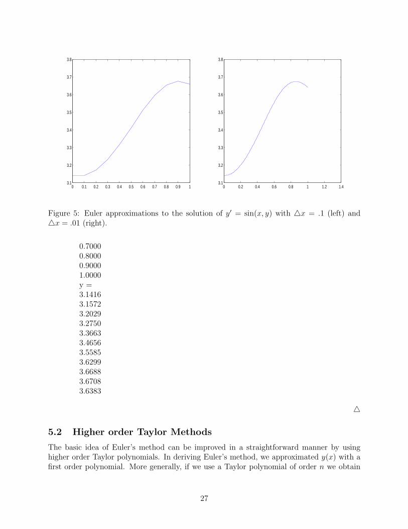
Figure 5: Euler approximations to the solution of y′ = sin(x, y) with △x = .1 (left) and△x = .01 (right).

0.70000.80000.90001.0000y =3.14163.15723.20293.27503.36633.46563.55853.62993.66883.67083.6383

△

5.2 Higher order Taylor Methods

The basic idea of Euler’s method can be improved in a straightforward manner by usinghigher order Taylor polynomials. In deriving Euler’s method, we approximated y(x) with afirst order polynomial. More generally, if we use a Taylor polynomial of order n we obtain

27

the Taylor method of order n. In order to see how this is done, we will derive the Taylormethod of order 2. (Euler’s method is the Taylor method of order 1.)

Again letting P = [x0, x1, ..., xn] denote a partition of the interval [x0, xn] on which wewould like to solve (7), our starting point for the Taylor method of order 2 is to write downthe Taylor polynomial of order 2 (with remainder) for y(xk+1) about the point xk. That is,according to Taylor’s theorem,

y(xk+1) = y(xk) + y′(xk)(xk+1 − xk) +y′′(xk)

2(xk+1 − xk)

2 +y′′′(c)

3!(xk+1 − xk)

3,

where c ∈ (xk, xk+1). As with Euler’s method, we drop off the error term (which is nowsmaller), and our approximation is

y(xk+1) ≈ y(xk) + y′(xk)(xk+1 − xk) +y′′(xk)

2(xk+1 − xk)

2.

We already know from our derivation of Euler’s method that y′(xk) can be replaced withf(xk, y(xk)). In addition to this, we now need an expression for y′′(xk). We can obtain thisby differentiating the original equation y′(x) = f(x, y(x)). That is,

y′′(x) =d

dxy′(x) =

d

dxf(x, y(x)) =

∂f

∂x(x, y(x)) +

∂f

∂y(x, y(x))

dy

dx,

where the last equality follows from a generalization of the chain rule to functions of twovariables (see Section 10.5.1 of the course text). From this last expression, we see that

y′′(xk) =∂f

∂x(xk, y(xk)) +

∂f

∂y(xk, y(xk))y

′(xk) =∂f

∂x(xk, y(xk)) +

∂f

∂y(xk, y(xk))f(xk, y(xk)).

Replacing y′′(xk) with the right-hand side of this last expression, and replacing y′(xk) withf(xk, y(xk)), we conclude

y(xk+1) ≈ y(xk) + f(xk, y(xk))(xk+1 − xk)

+[∂f

∂x(xk, y(xk)) +

∂f

∂y(xk, y(xk))f(xk, y(xk))

](xk+1 − xk)2

2.

If we take subintervals of equal width △x = (xk+1 − xk), this becomes

y(xk+1) ≈ y(xk) + f(xk, y(xk))△x

+[∂f

∂x(xk, y(xk)) +

∂f

∂y(xk, y(xk))f(xk, y(xk))

]△x2

2.

Example 5.2. Use the Taylor method of order 2 with n = 10 to approximate a solution tothe differential equation

dy

dx= sin(xy); y(0) = π,

on the interval [0, 1].

28

We will carry out the first few iterations by hand and leave the rest as a homeworkassignment. To begin, we observe that

f(x, y) = sin(xy)

∂f

∂x(x, y) = y cos(xy)

∂f

∂y(x, y) = x cos(xy).

If we let yk denote an approximation for y(xk), the Taylor method of order 2 becomes

yk+1 = yk + sin(xkyk)(.1)

+[

yk cos(xkyk) + xk cos(xkyk) sin(xkyk)](.1)2

2.

Beginning with the point (x0, y0) = (0, π), we compute

y1 = π + π(.005) = 3.1573,

which is closer to the correct value of 3.1572 than was the approximation of Euler’s method.We can now use the point (x1, y1) = (.1, 3.1573) to compute

y2 =3.1573 + sin(.1 · 3.1573)(.1)

+[

3.1573 cos(.1 · 3.1573) + .1 cos(.1 · 3.1573) sin(.1 · 3.1573)](.1)2

2=3.2035,

which again is closer to the correct value than was the y2 approximation for Euler’s method.△

5.3 Assignments

1. [5 pts] Alter the MATLAB M-file euler.m so that it employs the Taylor method of order2 rather than Euler’s method. Use your file with n = 10 to approximate the solution to thedifferential equation

dy

dx= sin(xy); y(0) = π,

on the interval [0, 1]. Turn in both your M-file and a list of values approximating y at0, .1, .2, .... Hint. Suppose you would like MATLAB to compute the partial derivative off(x, y) = sin(xy) and designate the result as the inline function fx. Use

>>syms x y;>>f=inline(’sin(x*y)’)f =Inline function:f(x,y) = sin(x*y)

29

>>fx=diff(f(x,y),x)fx =cos(x*y)*y>>fx=inline(char(fx))fx =Inline function:fx(x,y) = cos(x*y)*y

2. [5 pts] Proceeding similarly as in Section 5.2, derive the Taylor method of order 3.

30

6 Linear Algebra in MATLAB

MATLAB’s built-in solvers for systems of ODE return solutions as matrices, and so beforeconsidering these solvers we will briefly discuss MATLAB’s built-in tools for matrix manipu-lation. As suggested by its name, MATLAB (MATrix LABoratory) was originally developedas a set of numerical algorithms for manipulating matrices.

6.1 Defining and Referring to a Matrix

First, we have already learned how to define 1 × n matrices, which are simply row vectors.For example, we can define the 1 × 5 matrix

~v = [ 0 .2 .4 .6 .8 ]

with

>>v=[0 .2 .4 .6 .8]v =0 0.2000 0.4000 0.6000 0.8000>>v(1)ans =0>>v(4)ans =0.6000

We also see in this example that we can refer to the entries in v with v(1), v(2), etc.In defining a more general matrix, we proceed similarly by defining a series of row vectors,

ending each with a semicolon.

Example 6.1. Define the matrix

A =

1 2 34 5 67 8 9

in MATLAB.We accomplish this the following MATLAB code, in which we also refer to the entries

a21 and a12.

>>A=[1 2 3;4 5 6;7 8 9]A =1 2 34 5 67 8 9>>A(1,2)ans =

31

2>>A(2,1)ans =4

In general, we refer to the entry aij with A(i, j). We can refer to an entire column or anentire row by replacing the index for the row or column with a colon. In the following code,we refer to the first column of A and to the third row.

>>A(:,1)ans =147>>A(3,:)ans =7 8 9

△

6.2 Matrix Operations and Arithmetic

MATLAB adds and multiplies matrices according to the standard rules.

Example 6.2. For the matrices

A =

1 2 34 5 67 8 9

and B =

0 1 32 4 16 1 8

,

compute A + B, AB, and BA.Assuming A has already been defined in Example 9.1, we use

>>B=[0 1 3;2 4 1;6 1 8]B =0 1 32 4 16 1 8>>A+Bans =1 3 66 9 713 9 17>>A*Bans =22 12 2946 30 65

32

70 48 101>>B*Aans =25 29 3325 32 3966 81 96

In this example, notice the difference between AB and BA. While matrix addition is com-mutative, matrix multiplication is not. △

It is straightforward using MATLAB to compute several quantities regarding matrices,including the determinant of a matrix, the tranpose of a matrix, powers of a matrix, theinverse of a matrix, and the eigenvalues of a matrix.

Example 6.3. Compute the determinant, transpose, 5th power, inverse, and eigenvalues ofthe matrix

B =

0 1 32 4 16 1 8

.

Assuming this matrix has already been defined in Example 8.2, we use respectively

>>det(B)ans =-76>>B’ans =0 2 61 4 13 1 8Bˆ5ans =17652 7341 2757514682 6764 2260955150 22609 86096>>Bˆ(-1)ans =-0.4079 0.0658 0.14470.1316 0.2368 -0.07890.2895 -0.0789 0.0263>>inv(B)ans =-0.4079 0.0658 0.14470.1316 0.2368 -0.07890.2895 -0.0789 0.0263>>eig(B)ans =-1.9716

33

10.18813.7835

Notice that the inverse of B can be computed in two different ways, either as B−1 or withthe M-file inv.m. △

In addition to returning the eigenvalues of a matrix, the command eig will also returnthe associated eigenvectors. For a given square matrix A, the MATLAB command

[P, D] = eig(A)

will return a diagonal matrix D with the eigenvalues of A on the diagonal and a matrix Pwhose columns are made up of the eigenvectors of A. More precisely, the first column of Pwill be the eigenvector associated with d11, the second column of P will be the eigenvectorassociated with d22 etc.

Example 6.4. Compute the eigenvalues and eigenvectors for the matrix B from Example8.3.

We use

>>[P,D]=eig(B)P =-0.8480 0.2959 -0.03440.2020 0.2448 -0.96030.4900 0.9233 0.2767>>D =-1.9716 0 00 10.1881 00 0 3.7835

We see that the eigenvalue–eigenvector pairs of B are

−1.9716,

−.8480.2020.4900

; 10.1881,

.2959

.2448

.9233

; 3.7835,

−.0344−.9603.2767

.

Let’s check that these are correct for the first one. We should have B~v1 = −1.9716~v1. Wecan check this in MATLAB with the calculations

>>B*P(:,1)ans =1.6720-0.3982-0.9661>>D(1,1)*P(:,1)ans =1.6720-0.3982-0.9661

△

34

6.3 Solving Systems of Linear Equations

Example 6.5. Solve the linear system of equations

x1 + 2x2 + 7x3 = 1

2x1 − x2 = 3

9x1 + 5x2 + 4x3 = 0.

We begin by defining the coefficients on the left hand side as a matrix and the right handside as a vector. If

A =

1 2 72 −1 09 5 4

, ~x =

x1

x2

x3

and ~b =

130

,

then in matrix form this equation isA~x = ~b,

which is solved by~x = A−1~b.

In order to compute this in MATLAB, we use the following code.

>>A=[1 2 7;2 -1 0;9 5 4]A =1 2 72 -1 09 5 4>>b=[1 3 0]’b =130>>x=Aˆ(-1)*bx =0.6814-1.63720.5133>>x=A\bx =0.6814-1.63720.5133

Notice that MATLAB understands multiplication on the left by A−1, and interprets divisionon the left by A the same way. △

If the system of equations we want to solve has no solution or an infinite number ofsolutions, then A will not be invertible and we won’t be able to proceed as in Example 8.5.

35

In such cases (that is, when det A = 0), we can use the command rref, which reduces amatrix by Gauss–Jordan elimination.

Example 6.6. Find all solutions to the system of equations

x1 + x2 + 2x3 =1

x1 + x3 =2

2x1 + x2 + 3x3 =3.

In this case, we define the augmented matrix A, which includes the right-hand side. We have

>>A=[1 1 2 1;1 0 1 2;2 1 3 3]A =1 1 2 11 0 1 22 1 3 3>>rref(A)ans =1 0 1 20 1 1 -10 0 0 0

Returning to equation form, we have

x1 + x3 =2

x2 + x3 = − 1.

We have an infinite number of solutions

S = {(x1, x2, x3) : x3 ∈ R, x2 = −1 − x3, x1 = 2 − x3}.△

Example 6.7. Find all solutions to the system of equations

x1 + x2 + 2x3 =1

x1 + x3 =2

2x1 + x2 + 3x3 =2.

Proceeding as in Example 8.6, we use

>>A=[1 1 2 1;1 0 1 2;2 1 3 2]A =1 1 2 11 0 1 22 1 3 2>>rref(A)ans =1 0 1 00 1 1 00 0 0 1

36

In this case, we see immediately that the third equation asserts 0 = 1, which means there isno solution to this system. △

6.4 Assignments

1. [2 pts] For the matrix

A =

1 2 1−2 7 31 1 1

compute the determinant, transpose, 3rd power, inverse, eigenvalues and eigenvectors.

2. [2 pts] For matrix A from Problem 1, let P denote the matrix created from the eigenvectorsof A and compute

P−1AP.

Explain how the result of this calculation is related to the eigenvalues of A.

3. [2 pts] Find all solutions of the linear system of equations

x1 + 2x2 − x3 + 7x4 = 2

2x1 + x2 + 9x3 + 4x4 = 1

3x1 + 11x2 − x3 + 7x4 = 0

4x1 − 6x2 − x3 + 1x4 = − 1.

4. [2 pts] Find all solutions of the linear system of equations

−3x1 − 2x2 + 4x3 =0

14x1 + 8x2 − 18x3 =0

4x1 + 2x2 − 5x3 =0.

5. [2 pts] Find all solutions of the linear system of equations

x1 + 6x2 + 4x3 =1

2x1 + 4x2 − 1x3 =0

−x1 + 2x2 + 5x3 =0.

37

7 Solving ODE Numerically in MATLAB

MATLAB has a number of built-in tools for numerically solving ordinary differential equa-tions. We will focus on one of its most rudimentary solvers, ode45, which implements aversion of the Runge–Kutta 4th order algorithm. (This is essentially the Taylor method oforder 4, though implemented in an extremely clever way that avoids partial derivatives.) Fora complete list of MATLAB’s solvers, type helpdesk and then search for nonlinear numericalmethods.

7.1 First Order Equations

Example 7.1. Numerically approximate the solution of the first order differential equation

dy

dx= xy2 + y; y(0) = 1,

on the interval x ∈ [0, .5].For any differential equation in the form y′ = f(x, y), we begin by defining the function

f(x, y). For single equations, we can define f(x, y) as an inline function. Here,

>>f=inline(’x*yˆ2+y’)f =Inline function:f(x,y) = x*yˆ2+y

The basic usage for MATLAB’s solver ode45 is

ode45(function,domain,initial condition).

That is, we use

>>[x,y]=ode45(f,[0 .5],1)

and MATLAB returns two column vectors, the first with values of x and the second withvalues of y. (The MATLAB output is fairly long, so I’ve omitted it here.) Since x and y arevectors with corresponding components, we can plot the values with

>>plot(x,y)

which creates Figure 6.Choosing the partition. In approximating this solution, the algorithm ode45 has

selected a certain partition of the interval [0, .5], and MATLAB has returned a value of y ateach point in this partition. It is often the case in practice that we would like to specify thepartition of values on which MATLAB returns an approximation. For example, we mightonly want to approximate y(.1), y(.2), ..., y(.5). We can specify this by entering the vectorof values [0, .1, .2, .3, .4, .5] as the domain in ode45. That is, we use

38

0 0.1 0.2 0.3 0.4 0.5 0.6 0.71

1.1

1.2

1.3

1.4

1.5

1.6

1.7

1.8

1.9

2

Figure 6: Plot of the solution to y′ = xy2 + y, with y(0) = 1.

>>xvalues=0:.1:.5xvalues =0 0.1000 0.2000 0.3000 0.4000 0.5000>>[x,y]=ode45(f,xvalues,1)x =00.10000.20000.30000.40000.5000y =1.00001.11111.25001.42861.66672.0000

It is important to notice here that MATLAB continues to use roughly the same partition ofvalues that it originally chose; the only thing that has changed is the values at which it isprinting a solution. In this way, no accuracy is lost.

Options. Several options are available for MATLAB’s ode45 solver, giving the user lim-ited control over the algorithm. Two important options are relative and absolute tolerance,respecively RelTol and AbsTol in MATLAB. At each step of the ode45 algorithm, an error

39

is approximated for that step2. If yk is the approximation of y(xk) at step k, and ek is theapproximate error at this step, then MATLAB chooses its partition to ensure

ek ≤ max(RelTol ∗ yk, AbsTol),

where the default values are RelTol = .001 and AbsTol = .000001. In the event that yk

becomes large, the value for RelTol*yk will be large, and RelTol will need to be reduced.On the other hand, if yk becomes small, AbsTol will be relatively large and will need to bereduced.

For the equation y′ = xy2 + y, with y(0) = 1, the values of y get quite large as x nears1. In fact, with the default error tolerances, we find that the command

>>[x,y]=ode45(f,[0,1],1);

leads to an error message, caused by the fact that the values of y are getting too large as xnears 1. (Note at the top of the column vector for y that it is multipled by 1014.) In orderto fix this problem, we choose a smaller value for RelTol.

>>options=odeset(’RelTol’,1e-10);>>[x,y]=ode45(f,[0,1],1,options);>>max(y)ans =2.425060345544448e+07

In addition to employing the option command, I’ve computed the maximum value of y(x)to show that it is indeed quite large, though not as large as suggested by the previouscalculation. △

7.2 Systems of ODE

Solving a system of ODE in MATLAB is quite similar to solving a single equation, thoughsince a system of equations cannot be defined as an inline function, we must define it as anM-file.

Example 7.2. Solve the Lotka–Volterra predator–prey system

dy1

dt= ay1 − by1y2; y1(0) = y0

1

dy2

dt= − ry2 + cy1y2; y2(0) = y0

2,

with a = .5486, b = .0283, r = .8375, c = .0264, and y01 = 30, y0

2 = 4. (These valuescorrespond with data collected by the Hudson Bay Company between 1900 and 1920; seeSections 10 and 11 of these notes.)

In this case, we begin by writing the right hand side of this equation as the MATLABM-file lv.m:

2In these notes I’m omitting any discussion of how one computes these approximate errors. The basicidea is to keep track of the Taylor remainder terms that we discarded in Section 7 in our derivation of themethods.

40

function yprime = lv(t,y)%LV: Contains Lotka-Volterra equationsa = .5486;b = .0283;c = .0264;r = .8375;yprime = [a*y(1)-b*y(1)*y(2);-r*y(2)+c*y(1)*y(2)];

We can now solve the equations over a 20 year period as follows:

>>[t,y]=ode45(@lv,[0 20],[30;4])

The output from this command consists of a column of times and a matrix of populations.The first column of the matrix corresponds with y1 (prey in this case) and the secondcorresponds with y2 (predators). Suppose we would like to plot the prey population as afunction of time. In general, y(n, m) corresponds with the entry of y at the intersection ofrow n and column m, so we can refer to the entire first column of y with y(:, 1), where thecolon means all entries. In this way, Figure 7 can be created with the command

>>plot(t,y(:,1))

0 2 4 6 8 10 12 14 16 18 200

10

20

30

40

50

60

70

80

Figure 7: Prey populations as a function of time.

Similarly, we can plot the predator population along with the prey population with

>>plot(t,y(:,1),t,y(:,2),’–’)

where the predator population has been dashed (see Figure 8).Finally, we can plot an integral curve in the phase plane with

>>plot(y(:,1),y(:,2))

41

0 2 4 6 8 10 12 14 16 18 200

10

20

30

40

50

60

70

80

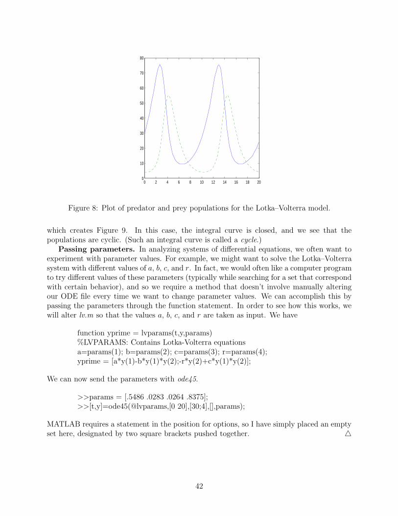
Figure 8: Plot of predator and prey populations for the Lotka–Volterra model.

which creates Figure 9. In this case, the integral curve is closed, and we see that thepopulations are cyclic. (Such an integral curve is called a cycle.)

Passing parameters. In analyzing systems of differential equations, we often want toexperiment with parameter values. For example, we might want to solve the Lotka–Volterrasystem with different values of a, b, c, and r. In fact, we would often like a computer programto try different values of these parameters (typically while searching for a set that correspondwith certain behavior), and so we require a method that doesn’t involve manually alteringour ODE file every time we want to change parameter values. We can accomplish this bypassing the parameters through the function statement. In order to see how this works, wewill alter lv.m so that the values a, b, c, and r are taken as input. We have

function yprime = lvparams(t,y,params)%LVPARAMS: Contains Lotka-Volterra equationsa=params(1); b=params(2); c=params(3); r=params(4);yprime = [a*y(1)-b*y(1)*y(2);-r*y(2)+c*y(1)*y(2)];

We can now send the parameters with ode45.

>>params = [.5486 .0283 .0264 .8375];>>[t,y]=ode45(@lvparams,[0 20],[30;4],[],params);

MATLAB requires a statement in the position for options, so I have simply placed an emptyset here, designated by two square brackets pushed together. △

42

0 10 20 30 40 50 60 70 800

10

20

30

40

50

60

Figure 9: Integral curve for the Lotka–Volterra equation.

7.3 Higher Order Equations

In order to solve a higher order equation numerically in MATLAB we proceed by first writingthe equation as a first order system and then proceeding as in the previous section.

Example 7.3. Solve the second order equation

y′′ + x2y′ − y = sin x; y(0) = 1, y′(0) = 3

on the interval x ∈ [0, 5].In order to write this equation as a first order system, we set y1(x) = y(x) and y2(x) =

y′(x). In this way,

y′1 = y2; y1(0) = 1

y′2 = y1 − x2y2 + sin x; y2(0) = 3,

which is stored in the MATLAB M-file secondode.m.

function yprime = secondode(x,y);%SECONDODE: Computes the derivatives of y 1 and y 2,%as a colum vectoryprime = [y(2); y(1)-xˆ2*y(2)+sin(x)];

We can now proceed with the following MATLAB code, which produces Figure 10.

>>[x,y]=ode45(@secondode,[0,5],[1;3]);>>plot(x,y(:,1))

43

0 0.5 1 1.5 2 2.5 3 3.5 4 4.5 50

2

4

6

8

10

12

14

Figure 10: Plot of the solution to y′′ + x2y′ − y = sin x; y(0) = 1, y′(0) = 3.

7.4 Assignments

1. [2 pts] Numerically approximate the solution of the first order differential equation

dy

dx=

x

y+ y; y(0) = 1,

on the interval x ∈ [0, 1]. Turn in a plot of your approximation.

2. [2 pts] Repeat Problem 1, proceeding so that MATLAB only returns values for x0 = 0,x1 = .1, x2 = .2, ..., x10 = 1. Turn in a list of values y(x1), y(x2) etc.

3. [2 pts] The logistic equation

dp

dt= rp(1 − p

K); p(0) = p0,

is solved by

pexact(t) =p0K

p0 + (K − p0)e−rt.

For parameter values r = .0215, K = 446.1825, and for initial value p0 = 7.7498 (consistentwith the U. S. population in millions), solve the logistic equation numerically for t ∈ [0, 200],and compute the error

E =200∑

t=1

(p(t) − pexact(t))2.

4. [2 pts] Repeat Problem 3 with RelTol = 10−10.

44

5. [2 pts] Numerically approximate the solution of the SIR epidemic model

dy1

dt= − by1y2; y1(0) = y0

1

dy2

dt= by1y2 − ay2; y2(0) = y0

2,

with parameter values a = .4362 and b = .0022 and initial values y01 = 762 and y0

2 = 1. Turnin a plot of susceptibles and infectives as a function of time for t ∈ [0, 20]. Also, plot y2 asa function of y1, and discuss how this plot corresponds with our stability analysis for thisequation. Check that the maximum of this last plot is at a

b, and give values for Sf and SR

as defined in class.

45

8 Graphing Functions of Two Variables

In this section we will begin to get a feel for functions of two variables by plotting a numberof functions with MATLAB. In the last subsection we will employ what we’ve learned todevelop a geometric interpretation of partial derivatives.

8.1 Surface Plots

For a given function of two variables f(x, y) we can associate to each pair (x, y) a thirdvariable z = f(x, y) and in this way create a collection of points (x, y, z) that describe asurface in three dimensions.

Example 8.1. Plot a graph of the function

f(x, y) = x2 + 4y2

for x ∈ [−2, 2] and y ∈ [−1, 1].MATLAB provides a number of different tools for plotting surfaces, of which we will

only consider surf . (Other options include surfc, surfl, ezsurf, mesh, meshz, meshc, ezmesh.)In principle, each tool works the same way: MATLAB takes a grid of points (x, y) in thespecified domain, computes z = f(x, y) at each of these points, and then plots the surfacedescribed by the resulting points (x, y, z). Given a vector of x values and a vector of y values,the command meshgrid creates such a mesh. In the following MATLAB code we will usethe surf command to create Figure 11.

>>x=linspace(-2,2,50);>>y=linspace(-1,1,50);>>[x,y]=meshgrid(x,y);>>z=x.ˆ2+4*y.ˆ2;>>surf(x,y,z)>>xlabel(’x’); ylabel(’y’); zlabel(’z’);

Here, the last command has been entered after the figure was minimized. Observe here thatone tool in the graphics menu is a rotation option that allows us to look at the surface fromseveral different viewpoints. Two different views are given in Figure 11. (These figures willappear in color in your MATLAB graphics window, and the different colors correspond withdifferent levels of z.) △Example 8.2. Plot the ellipsoid described by the equation

x2

4+

y2

16+

z2

9= 1,

for appropriate values of x and y.In this case the surface is described implicitly, though we can describe it explicitly as the

two functions

z− = − 3

√

1 − x2

4− y2

9

z+ = + 3

√

1 − x2

4− y2

9.

46

−2−1

01

2

−1

−0.5

0

0.5

10

2

4

6

8

xy

z

−2 −1 0 1 2−1

010

1

2

3

4

5

6

7

8

xy

zFigure 11: Graph of the paraboloid for f(x, y) = x2 + 4y2 (two views).

The difficulty we would have with proceeding as in the previous example is that the appro-priate domain of x and y values is the ellipse described by

x2

4+

y2

16≤ 1,

and meshgrid defines a rectangular domain. Fortunately, MATLAB has a built-in functionellipsoid that creates a mesh of points (x, y, z) an the surface of an ellipsoid described bythe general equation

(x − a)2

A2+

(y − b)2

B2+

(z − c)2

C2= 1.

The syntax is[x,y,z]=ellipsoid(a,b,c,A,B,C,n),

where n is an optional parameter (n = 20, by default) that sets the matrix of values describingeach variable to be (n + 1) × (n + 1). Figure 12 with the following MATLAB code.

>>[x,y,z]=ellipsoid(0,0,0,2,4,3);>>surf(x,y,z)

△Example 8.3. Plot the hyperboloid of one sheet descibed by the equation

x2

4− y2

16+ z2 = 1.

As in Example 12.2, we run into a problem of specifying an appropriate domain of points(x, y), except that in this case MATLAB does not have (that I’m aware of) a built-in function

47

−2−1

01

2

−4

−2

0

2

4−3

−2

−1

0

1

2

3

Figure 12: Ellipsoid described by x2

4+ y2

16+ z2

9= 1.

for graphing hyperbolas. Nonetheless, we can proceed by specifying the values x, y, and zparametrically. First, recall the hyperbolic trigonometric functions

cosh s =es + e−s

2

sinh s =es − e−s

2.

The following identity is readily verified: cosh2 s − sinh2 s = 1. If we additionally use theidentity cos2 t + sin2 t = 1, then we find

cosh2(s) cos2(t) − sinh2(s) + cosh2(s) sin2(t) = 1.

What this means is that if we make the substitutions

x = 2 cosh(s) cos(t)

y = 4 sinh(s)

z = cosh(s) sin(t),

thenx2

4− y2

16+ z2 =

4 cosh2(s) cos2(t)

4− 16 sinh2(s)

16+ cosh2(s) sin2(t) = 1.

That is, these values of x, y, and z solve our equation. It is natural now to take t ∈ [0, 2π]so that the cosine and sine functions will taken on all values between -1 and +1. The largerthe interval we choose for s the larger the more of the manifold we’ll plot. In this case, let’stake s ∈ [−1, 1]. We can now create Figure 13 with the followoing MATLAB code.

48

>>s=linspace(-1,1,25);>>t=linspace(0,2*pi,50);>>[s,t]=meshgrid(s,t);>>x=2*cosh(s).*cos(t);>>y=4*sinh(s);>>z=cosh(s).*sin(t);>>surf(x,y,z)

−4−2

02

4

−5

0

5−2

−1

0

1

2

Figure 13: Plot of the surface for x2

4− y2

16+ z2 = 1.

Of course the ellipsoid plotted in Example 12.2 could similarly have been plotted withthe parametrization

x =2 sin(s) cos(t)

y =4 sin(s) sin(t)

z =3 cos(s),

and s ∈ [0, π], t ∈ [0, 2π]. △

8.2 Geometric Interpretation of Partial Derivatives

For a function of one variable f(x), the derivative at a value x = a has a very simplegeometric interpretation as the slope of the line that is tangent to the graph of f(x) at thepoint (a, f(a)). In particular, if we write the equation for this tangent line in the point–slopeform

y − y0 = m(x − x0),

49

then the slope is m = f ′(a) and the point of tangency is (x0, y0) = (a, f(a)), and so we have

y − f(a) = f ′(a)(x − a).

In this subsection our goal will be to point out a similar geometric interpretation for functionsof two variables. (Though we’ll also say something about the case of three and more variables,the geometry is difficult to envision in those cases.)

When we consider the geometry of a function of two variables we should replace theconcept of a tangent line with that of a tangent plane. As an extremely simple exampleto ground ourselves with, consider the parabaloid depicted in Figure 11, and the point atthe origin (0, 0, 0). The tangent plane to the surface at this point is the x-y plane. (Thenotion of precisely what we mean by a tangent plane will emerge from this discussion, butjust so we’re not chasing our tails, here’s a version of it that does not involve derivatives:The tangent plane at a point P is defined as the plane such that for any sequence of points{Pn} on the surface S such that Pn → P as n → ∞, the angles between the lines PPn andthe plane approach 0.)

In order to determine an equation for the plane tangent to the graph of f(x, y) at thepoint (x0, y0, f(x0, y0)), we first recall that just as every line can be written in the point–slopeform y − y0 = m(x − x0) every plane can be written in the form

z − z0 = m1(x − x0) + m2(y − y0),

where (x0, y0, z0) is a point on the plane. In order to find the value of m1, we set y = y0, sothat z becomes a function of the single variable x:

z = f(x, y0).

The line that is tangent to the graph of f(x, y0) at x = x0 can be written in the point-slopeform

z − z0 = m1(x − x0),

where

m1 =∂f

∂x(x0, y0).

Likewise, we find that

m2 =∂f

∂y(x0, y0),

and so the equation for the tangent plane is

z − z0 =∂f

∂x(x0, y0)(x − x0) +

∂f

∂y(x0, y0)(y − y0).

We conclude that ∂f∂x

(x0, y0) is a measure of the incline of the tangent plane in the x direction,

while ∂f∂y

(x0, y0) is a measure of this incline in the y direction.

Example 8.4. Find the equation for the plane that is tangent to the paraboloid discussed inExample 12.1 at the point (x0, y0) = (1, 1

2) and plot this tangent plane along with a surface

plot of the function.

50

First, we observe that for (x0, y0) = (1, 12), we have z0 = 1 + 1 = 2. Additionally,

∂f

∂x= 2x ⇒ ∂f

∂x(1,

1

2) = 2

∂f

∂y= 8y ⇒ ∂f

∂y(1,

1

2) = 4.

The equation of the tangent plane is therefore

z − 2 = 2(x − 1) + 4(y − 1

2),

orz = 2x + 4y − 2.

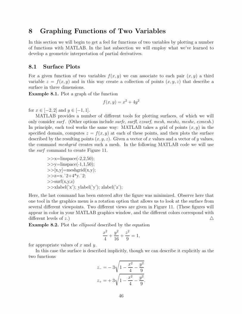
We can now create Figure 14 with the following MATLAB code (an additional view has beenadded by a rotation in the graphics menu):

>>x=linspace(-2,2,50);>>y=linspace(-1,1,50);>>[x,y]=meshgrid(x,y);>>z=x.ˆ2+4*y.ˆ2;>>tplane=2*x+4*y-2;>>surf(x,y,z)>>hold on>>surf(x,y,tplane)

△

−2−1

01

2

−1

−0.5

0

0.5

1−10

−5

0

5

10

−2−1

01

2

−1

−0.5

0

0.5

1

−10

−5

0

5

10

Figure 14: Graph of f(x, y) = x2 + 4y2 along with the tangent plane at (1, 12) (two views).

51

8.3 Assignments

1. [2 pts] Create a surface plot for the function

f(x, y) = x2 − 4y2

for x ∈ [−2, 2] and y ∈ [−1, 1]. Print two different views of your figure. (The result is ahyperbolic paraboloid, for which the point (0, 0, 0) is a saddle point.)

2. [2 pts] Plot the ellipse described by the equation

x2

34.81+

y2

10.5625+

z2

10.5625= 1.

(These are the dimensions in inches of a standard (American) football.)

3. [3 pts] Plot the surface described by the equation

x2

4− y2

16− z2 = 1.

Hint. Observe the identity

cosh2(s) − sinh2(s) cos2(t) − sinh2(s) sin2(t) = 1.

This surface is called a hyperboloid of two sheets, so be sure your figure has two separatesurfaces.

4. [3 pts] Along with your hyperbolic paraboloid from Problem 1, plot the plane that istangent to your surface at the point (x, y) = (1, 1

2).

52

9 Least Squares Regression

9.1 Data Fitting in MATLAB

One important application of maximization/minimization techniques is to the study of datafitting and parameter estimation.

Example 9.1. Suppose the Internet auctioneer, eBay, hires us to predict its net income forthe year 2003, based on its net incomes for 2000, 2001, and 2002 (see Table 1).

Year Net Income

2000 48.3 million2001 90.4 million2002 249.9 million

Table 1: Yearly net income for eBay.

We begin by simply plotting this data as a scatterplot of points. In MATLAB, we developFigure 15 through the commands,

>>year=[0 1 2];>>income=[48.3 90.4 249.9];>>plot(year,income,’o’)>>axis([-.5 2.5 25 275])

−0.5 0 0.5 1 1.5 2 2.5

50

100

150

200

250

EBAY net income data 2000−2002

Year

Ne

t In

co

me

Figure 15: Net Income by year for eBay.

Our first approach toward predicting eBay’s future profits might be to simply find acurve that best fits this data. The most common form of curve fitting is linear least squares

53

regression. Before discussing the details of this method, we will get some idea of the goalof it by carrying out a calculation in MATLAB. At this point the only thing we need tounderstand regarding the underlying mathematics is that our goal is to find a polynomialthat fits our data in some reasonable sense. The MATLAB command for polynomial fittingis polyfit(x,y,n), where x and y are vectors and n is the order of the polynomial. For example,if we would like to fit the eBay data with a straight line (a polynomial of order 1), we have

>>polyfit(year,income,1)ans =100.8000 28.7333

Notice particularly that, left to right, MATLAB returns the coefficient of the highest powerof x first, the second highest power of x second etc., continuing until the y-intercept is givenlast. Our model for the eBay data is

y = 100.8x + 28.7333,

where x denotes the year and y denotes the net income. Alternatively, for polynomial fittingup to order 10, MATLAB has the option of choosing it directly from the graphics menu.In the case of our eBay data, while Figure 15 is displayed in MATLAB, we choose Tools,Basic Fitting. A new window opens and offers a number of fitting options. We can easilyexperiment by choosing the linear option and then the quadratic option, and comparing.(Since we only have three data points in this example, the quadratic fit necessarily passesthrough all three. This, of course, does not mean that the quadratic fit is best, only that weneed more data.) For this small a set of data, the linear fit is safest, so select that one andclick on the black arrow at the bottom right corner of the menu. Checking that the fit givenin the new window is linear, select the option Save to Workspace. MATLAB saves thepolynomial fit as a structure, which is a MATLAB array variable that can hold data of varyingtypes; for example, a string as its first element and a digit as its second and so on. Theelements of a structure can be accessed through the notation structurename.structureelement.Here, the default structure name is fit, and the first element is type. The element fit.typecontains a string describing the structure. The second element of the structure is fit.coeff,which contains the polynomial coefficients of our fit. Finally, we can make a prediction withthe MATLAB command polyval,

>>polyval(fit.coeff,3)

for which we obtain the prediction 331.1333. Finally, we mention that MATLAB refers tothe error for its fit as the norm of residuals, which is precisely the square root of the errorE that we will define below. △

9.2 Polynomial Regression

In this section, we will develop the technique of least squares regression. To this end, thefirst thing we need is to specify what we mean by “best fit” in this context. Consider thethree points of data given in Example 13.1, and suppose we would like to draw a line through

54

−0.5 0 0.5 1 1.5 2 2.5

50

100

150

200

250

EBAY net income data 2000−2002

Year

Ne

t In

co

me

(x2,y

2)

E2=|y

2−mx

2−b|

Figure 16: Least squares vertical distances.

these points in such a way that the distance between the points and the line is minimized(see Figure 16).

Labeling these three points (x1, y1), (x2, y2), and (x3, y3), we observe that the verticaldistance between the line and the point (x2, y2) is given by the error E2 = |y2 − mx2 − b|.The idea behind the least squares method is to sum these vertical distances and minimize thetotal error. In practice, we square the errors both to keep them positive and to avoid possibledifficulty with differentiation (recall that absolute values can be subtle to differentiate), whichwill be required for minimization. Our total least squares error becomes

E(m, b) =n

∑

k=1

(yk − mxk − b)2.

In our example, n = 3, though the method remains valid for any number of data points.We note here that in lieu of these vertical distances, we could also use horizontal distances

between the points and the line or direct distances (the shortest distances between the pointsand the line). While either of these methods could be carried out in the case of a line, theyboth become considerably more complicated in the case of more general cures. In the case ofa parabola, for example, a point would have two different horizontal distances from the curve,and while it could only have one shortest distance to the curve, computing that distancewould be a fairly complicted problem in its own right.

Returning to our example, our goal now is to find values of m and b that minimize theerror function E(m, b). In order to maximize or minimize a function of multiple variables,we compute the partial derivative with respect to each variable and set them equal to zero.

55

Here, we compute

∂

∂mE(m, b) = 0

∂

∂bE(m, b) = 0.

We have, then,

∂

∂mE(m, b) = − 2

n∑

k=1

xk(yk − mxk − b) = 0,

∂

∂bE(m, b) = − 2

n∑

k=1

(yk − mxk − b) = 0,

which we can solve as a linear system of two equations for the two unknowns m and b.Rearranging terms and dividing by 2, we have

m

n∑

k=1

x2k + b

n∑

k=1

xk =

n∑

k=1

xkyk,

m

n∑

k=1

xk + b

n∑

k=1

1 =

n∑

k=1

yk. (10)

Observing that∑n

k=1 1 = n, we multiply the second equation by 1n

∑nk=1 xk and subtract it

from the first to get the relation,

m(

n∑

k=1

x2k −

1

n(

n∑

k=1

xk)2)

=

n∑

k=1

xkyk −1

n(

n∑

k=1

xk)(

n∑

k=1

yk),

or

m =

∑nk=1 xkyk − 1

n(∑n

k=1 xk)(∑n

k=1 yk)∑n

k=1 x2k − 1

n(∑n

k=1 xk)2.

Finally, substituting m into equation (10), we have

b =1

n

n∑

k=1

yk − (n

∑

k=1

xk)

∑nk=1 xkyk − 1

n(∑n

k=1 xk)(∑n

k=1 yk)

n∑n

k=1 x2k − (

∑nk=1 xk)2

=(∑n

k=1 yk)(∑n

k=1 x2k) − (

∑nk=1 xk)(

∑nk=1 xkyk)

n∑n

k=1 x2k − (

∑nk=1 xk)2

.

We can verify that these values for m and b do indeed constitute a minimum by observingthat by continuity there must be at least one local minimum for E, and that since m and bare uniquely determined this must be it. Alternatively, we have the following theorem.

Theorem 9.1. Suppose f(x, y) is differentiable in both independent variables on some do-main D ⊂ R

2 and that (a, b) is an interior point of D for which

fx(a, b) = fy(a, b) = 0.

56

If moreover fxx, fxy, fyx, and fyy exist at the point (a, b), then the nature of (a, b) can bedetermined from

D = fxx(a, b)fyy(a, b) − fxy(a, b)2

as follows:1. If D > 0 and fxx(a, b) > 0, then f has a relative minimum at (a, b);2. If D > 0 and fxx(a, b) < 0, then f has a relative maximum at (a, b);3. If D < 0, then f has neither a maximum nor a minimum at (a, b);4. If D = 0, further analysis is required, and any of 1–3 remain possible.

Notice particularly that in the event that D > 0, this looks very much like the relatedsecond-derivative test for functions of a single independent variable.

Observe finally that we can proceed similarly polynomials of higher order. For example,for second order polynomials with general form y = a0 + a1x + a2x

2, our error becomes

E(a0, a1, a2) =

n∑

k=1

(yk − a0 − a1xk − a2x2k)

2.

In this case, we must compute a partial derivative of E with respect to each of three pa-rameters, and consequently (upon differentiation) solve three linear equations for the threeunknowns.

We conclude this section with an example in which the best fit polynomial is quadratic.

Example 9.2. (Crime and Unemployment.) Table 2 contains data relating crime rate per100,000 citizens to percent unemployment during the years 1994–2000. In this example, wewill find a polynomial that describes crime rate as a function of percent unemployment.

Year Crime Rate Percent Unemployment

1994 5,373.5 6.1%1995 5,277.6 5.6%1996 5,086.6 5.4%1997 4,922.7 4.9%1998 4,619.3 4.5%1999 4,266.8 4.2%2000 4,124.8 4.0%

Table 2: Crime rate and unemployment data.

We begin by plotting these points with crime rates on the y-axis and percent unemploy-ment on the x-axis. The following MATLAB code creates Figure 17.

>>x=[6.1 5.6 5.4 4.9 4.5 4.2 4.0];>>y=[5373.5 5277.6 5086.6 4922.7 4619.3 4266.8 4124.8];>>plot(x,y,’o’)

Proceeding from the Tools, Data Fitting option in the graphics menu (as in Example13.1), we try both the linear and the quadratic fit and find that the quadratic fit is muchbetter (see Figure 18). Though we haven’t yet quantitatively developed the socioeconomicreasons for this particular relation,3 we do have a genuinely predictive model. For example,

3And don’t worry, we’re not going to.

57

4 4.5 5 5.5 6 6.54000

4200

4400

4600

4800

5000

5200

5400

Figure 17: Scatterplot of crime rate versus unemployment.

the percent unemployment in 2001 was 4.8%, and so if we save our quadratic fit to theworkplace as fit2, we can predict that the crime rate was 4,817.8 as follows4:

>>polyval(fit2.coeff,4.8)ans =4.8178e+03

△

9.3 Regression with more general functions

Example 9.3. Let’s consider population growth in the United States, beginning with thefirst government census in 1790 (see Table 3).

Year 1790 1800 1810 1820 1830 1840 1850 1860 1870 1880 1890 1900

Pop 3.93 5.31 7.24 9.64 12.87 17.07 23.19 31.44 39.82 50.16 62.95 75.99

Year 1910 1920 1930 1940 1950 1960 1970 1980 1990 2000

Pop 91.97 105.71 122.78 131.67 151.33 179.32 203.21 226.50 249.63 281.42

Table 3: Population data for the United States, 1790–2000, measured in millions.

If we let p(t) represent the population at time t, the logistic model of population growthis given by

dp

dt= rp(1 − p

K); p(0) = p0 (11)

4As it turns out, this isn’t a very good prediction, because there was a lag between the increase in percentemployment (from 4% in 2000 to 4.8% in 2001) and the increase in crime rate, which only increased from4124.8 in 2000 to 4,160.5 in 2001.

58

4 4.5 5 5.5 6 6.54000

4200

4400

4600

4800

5000

5200

5400

5600

5800

Percent Unemployment

Crim

e R

ate

pe

r 1

00

,00

0 in

ha

bita

nts

Crime Rate versus Unemployment

y = 6.1e+02*x + 1.8e+03y = − 2.2e+02*x2 + 2.8e+03*x − 3.6e+03

data 1 linear quadratic

Figure 18: Best fit curves for crime–unemployment data.

where p0 represents the initial population of the inhabitants, r is called the “growth rate”of the population, and K is called the “carrying capacity.” Observe that while the rate atwhich the population grows is assumed to be proportional to the size of the population,the population is assumed to have a maximum possible number of inhabitants, K. (If p(t)ever grows larger than K, then dp

dtwill become negative and the population will decline.)

Equation (11) can be solved by separation of variables and partial fractions, and we find

p(t) =p0K

(K − p0)e−rt + p0

. (12)

Though we will take year 0 to be 1790, we will assume the estimate that year was fairlycrude and obtain a value of p0 by fitting the entirety of the data. In this way, we have threeparameters to contend with, and carrying out the full regression analysis would be tedious.

The first step in finding values for our parameters with MATLAB consists of writing ourfunction p(t) as an M-file, with our three parameters p0, r, and K stored as a parametervector p = (p(1), p(2), p(3)):

function P = logistic(p,t);%LOGISTIC: MATLAB function file that takes%time t, growth rate r (p(1)),%carrying capacity K (p(2)),%and initial population P0 (p(3)), and returns%the population at time t.P = p(2).*p(3)./((p(2)-p(3)).*exp(-p(1).*t)+p(3));

MATLAB’s function lsqcurvefit() can now be employed at the Command Window, as follows.

59

>>decades=0:10:210;>>pops=[3.93 5.31 7.24 9.64 12.87 17.07 23.19 31.44 39.82 50.16 62.95 75.99...91.97 105.71 122.78 131.67 151.33 179.32 203.21 226.5 249.63 281.42];>>p0 = [.01 1000 3.93];>>[p,error]=lsqcurvefit(@logistic,p0,decades,pops)Maximum number of function evaluations exceeded;increase options.MaxFunEvalsp =0.0206 485.2402 8.4645error =464.1480>>sqrt(error)ans =21.5441

After defining the data, we have entered our initial guess as to what the parameters shouldbe, the vector p0. (Keep in mind that MATLAB is using a routine similar to fzero() to solvethe system of nonlinear algebraic equations, and typically can only find roots reasonably nearyour guesses.) In this case, we have guessed a small value of r corresponding very roughly tothe fact that we live 70 years and have on average (counting men and women) 1.1 childrenper person5 (r ∼= 1/70), a population carrying capacity of 1 billion, and an initial populationequal to the census data. Finally, we use lsqcurvefit(), entering respectively our function file,our initial parameter guesses, and our data. The function lsqcurvefit() renders two outputs:our parameters and a sum of squared errors, which we have called error. Though the errorlooks enormous, keep in mind that this is a sum of all errors squared,

error =∑

decades

(pops(decade)-modelpops(decade))2.

A more reasonable measure of error is the square root of this, from which we see that over22 decades our model is only off by around 21.54 million people. In this case, MATLABhas not closed its iteration completely, and returns the error message, Maximum number offunction evaluations exceeded. In order to avoid this, let’s refine our code by increasing thenumber of function evaluations MATLAB should carry out. We have

>>lowerbound = [0 0 0];>>options = optimset(’MaxFunEvals’,10000);>>[p,error]=lsqcurvefit(@logistic,p0,decades,pops,lowerbound,[],options)Optimization terminated successfully:Relative function value changing by less than OPTIONS.TolFunp =0.0215 446.1825 7.7498error =440.9991

5According to census 2000.

60

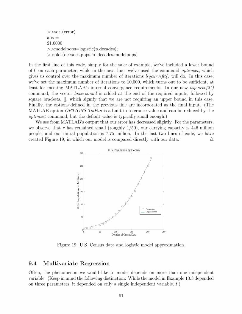
>>sqrt(error)ans =21.0000>>modelpops=logistic(p,decades);>>plot(decades,pops,’o’,decades,modelpops)

In the first line of this code, simply for the sake of example, we’ve included a lower boundof 0 on each parameter, while in the next line, we’ve used the command optimset , whichgives us control over the maximum number of iterations lsqcurvefit() will do. In this case,we’ve set the maximum number of iterations to 10,000, which turns out to be sufficient, atleast for meeting MATLAB’s internal convergence requirements. In our new lsqcurvefit()command, the vector lowerbound is added at the end of the required inputs, followed bysquare brackets, [], which signify that we are not requiring an upper bound in this case.Finally, the options defined in the previous line are incorporated as the final input. (TheMATLAB option OPTIONS.TolFun is a built-in tolerance value and can be reduced by theoptimset command, but the default value is typically small enough.)

We see from MATLAB’s output that our error has decreased slightly. For the parameters,we observe that r has remained small (roughly 1/50), our carrying capacity is 446 millionpeople, and our initial population is 7.75 million. In the last two lines of code, we havecreated Figure 19, in which our model is compared directly with our data. △

0 50 100 150 200 2500

50

100

150

200

250

300U. S. Population by Decade

Decades of Census Data

U.

S.

Po

pu

latio

ns in

Mill

ion

s

Census dataLogistic model

Figure 19: U.S. Census data and logistic model approximation.

9.4 Multivariate Regression

Often, the phenomenon we would like to model depends on more than one independentvariable. (Keep in mind the following distinction: While the model in Example 13.3 dependedon three parameters, it depended on only a single independent variable, t.)

61

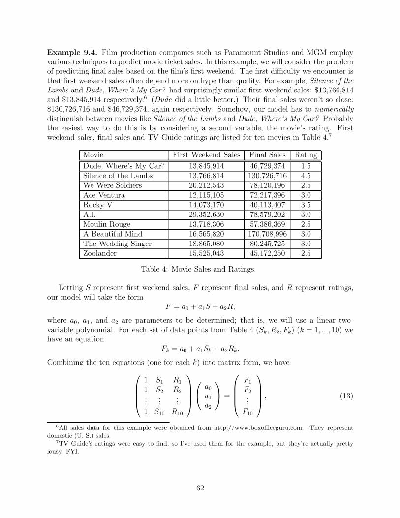
Example 9.4. Film production companies such as Paramount Studios and MGM employvarious techniques to predict movie ticket sales. In this example, we will consider the problemof predicting final sales based on the film’s first weekend. The first difficulty we encounter isthat first weekend sales often depend more on hype than quality. For example, Silence of theLambs and Dude, Where’s My Car? had surprisingly similar first-weekend sales: $13,766,814and $13,845,914 respectively.6 (Dude did a little better.) Their final sales weren’t so close:$130,726,716 and $46,729,374, again respectively. Somehow, our model has to numericallydistinguish between movies like Silence of the Lambs and Dude, Where’s My Car? Probablythe easiest way to do this is by considering a second variable, the movie’s rating. Firstweekend sales, final sales and TV Guide ratings are listed for ten movies in Table 4.7

Movie First Weekend Sales Final Sales Rating

Dude, Where’s My Car? 13,845,914 46,729,374 1.5Silence of the Lambs 13,766,814 130,726,716 4.5We Were Soldiers 20,212,543 78,120,196 2.5Ace Ventura 12,115,105 72,217,396 3.0Rocky V 14,073,170 40,113,407 3.5A.I. 29,352,630 78,579,202 3.0Moulin Rouge 13,718,306 57,386,369 2.5A Beautiful Mind 16,565,820 170,708,996 3.0The Wedding Singer 18,865,080 80,245,725 3.0Zoolander 15,525,043 45,172,250 2.5

Table 4: Movie Sales and Ratings.

Letting S represent first weekend sales, F represent final sales, and R represent ratings,our model will take the form

F = a0 + a1S + a2R,

where a0, a1, and a2 are parameters to be determined; that is, we will use a linear two-variable polynomial. For each set of data points from Table 4 (Sk, Rk, Fk) (k = 1, ..., 10) wehave an equation

Fk = a0 + a1Sk + a2Rk.

Combining the ten equations (one for each k) into matrix form, we have

1 S1 R1

1 S2 R2...

......

1 S10 R10

a0

a1

a2

=

F1

F2...

F10

, (13)

6All sales data for this example were obtained from http://www.boxofficeguru.com. They representdomestic (U. S.) sales.

7TV Guide’s ratings were easy to find, so I’ve used them for the example, but they’re actually prettylousy. FYI.

62

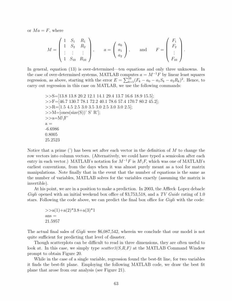
or Ma = F , where

M =

1 S1 R1

1 S2 R2...

......

1 S10 R10

, a =

a0

a1

a2

, and F =

F1

F2...

F10

.

In general, equation (13) is over-determined—ten equations and only three unknowns. Inthe case of over-determined systems, MATLAB computes a = M−1F by linear least squaresregression, as above, starting with the error E =

∑10k=1(Fk − a0 − a1Sk − a2Rk)

2. Hence, tocarry out regression in this case on MATLAB, we use the following commands:

>>S=[13.8 13.8 20.2 12.1 14.1 29.4 13.7 16.6 18.9 15.5];>>F=[46.7 130.7 78.1 72.2 40.1 78.6 57.4 170.7 80.2 45.2];>>R=[1.5 4.5 2.5 3.0 3.5 3.0 2.5 3.0 3.0 2.5];>>M=[ones(size(S))’ S’ R’];>>a=M\F’a =-6.69860.800525.2523

Notice that a prime (’) has been set after each vector in the definition of M to change therow vectors into column vectors. (Alternatively, we could have typed a semicolon after eachentry in each vector.) MATLAB’s notation for M−1F is M\F, which was one of MATLAB’searliest conventions, from the days when it was almost purely meant as a tool for matrixmanipulations. Note finally that in the event that the number of equations is the same asthe number of variables, MATLAB solves for the variables exactly (assuming the matrix isinvertible).

At his point, we are in a position to make a prediction. In 2003, the Affleck–Lopez debacleGigli opened with an initial weekend box office of $3,753,518, and a TV Guide rating of 1.0stars. Following the code above, we can predict the final box office for Gigli with the code:

>>a(1)+a(2)*3.8+a(3)*1ans =21.5957

The actual final sales of Gigli were $6,087,542, wherein we conclude that our model is notquite sufficient for predicting that level of disaster.

Though scatterplots can be difficult to read in three dimensions, they are often useful tolook at. In this case, we simply type scatter3(S,R,F) at the MATLAB Command Windowprompt to obtain Figure 20.

While in the case of a single variable, regression found the best-fit line, for two variablesit finds the best-fit plane. Employing the following MATLAB code, we draw the best fitplane that arose from our analysis (see Figure 21).

63

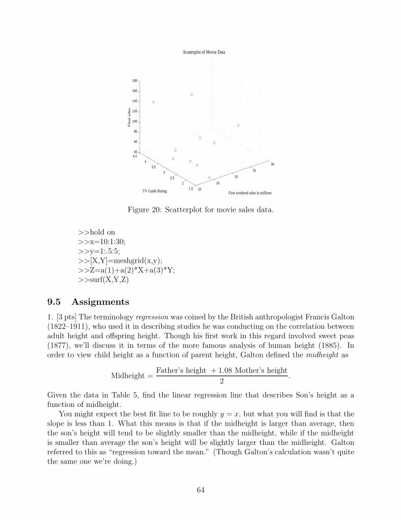
10

15

20

25

30

1.5

2

2.5

3

3.5

4

4.540

60

80

100

120

140

160

180

First weekend sales in millionsTV Guide Rating

Fin

al sa

les

Scatterplot of Movie Data

Figure 20: Scatterplot for movie sales data.

>>hold on>>x=10:1:30;>>y=1:.5:5;>>[X,Y]=meshgrid(x,y);>>Z=a(1)+a(2)*X+a(3)*Y;>>surf(X,Y,Z)

9.5 Assignments

1. [3 pts] The terminology regression was coined by the British anthropologist Francis Galton(1822–1911), who used it in describing studies he was conducting on the correlation betweenadult height and offspring height. Though his first work in this regard involved sweet peas(1877), we’ll discuss it in terms of the more famous analysis of human height (1885). Inorder to view child height as a function of parent height, Galton defined the midheight as

Midheight =Father’s height + 1.08 Mother’s height

2.

Given the data in Table 5, find the linear regression line that describes Son’s height as afunction of midheight.

You might expect the best fit line to be roughly y = x, but what you will find is that theslope is less than 1. What this means is that if the midheight is larger than average, thenthe son’s height will tend to be slightly smaller than the midheight, while if the midheightis smaller than average the son’s height will be slightly larger than the midheight. Galtonreferred to this as “regression toward the mean.” (Though Galton’s calculation wasn’t quitethe same one we’re doing.)

64

10

15

20

25

30

1

2

3

4

520

40

60

80

100

120

140

160

180

First weekend sales in millions

Scatterplot of Movie Data

TV Guide Rating

Fin

al sa

les

Figure 21: Movie sales data along with best-fit plane.

2. [3 pts] The Gompertz model for population growth is described by the equation

dp

dt= −rp ln(

p

K); p(0) = p0,

which (as we will show next semester) can be solved by the function

p(t) = K(p0

K)e−rt

.

Using the U.S. population data from Example 13.3, estimate values for r, K, and p0, andplot your model along with the data.

3. [4 pts] An alternative approach to the fit we carried out in Problem 1 would be amultivariate fit with

C = a0 + a1M + a2F,

where C denotes child’s height, M denotes mother’s height, and F denotes father’s height.Find values for a0, a1, and a2 for this fit. According to this model, which height is moresignificant for a son’s height, the mother’s or the father’s.

65

Mother’s height Father’s height Son’s height

65 67 6860 70 6770 72 7462 70 6963 67 6864 71 7064 69 6961 68 6765 70 7066 73 70

Table 5: Child and Parent Heights.

10 Estimating Parameters in Discrete Time Models

In many cases, we would like to find parameter values for a discrete time model even whenwe cannot write down an explicit solution to the model. In such cases we can still use leastsquares regression if we solve the equation numerically each time we need to evaluate it.While computationally expensive (i.e., time consuming), this process can give very goodresults.

Example 10.1. Given the U. S. population data in Table 3 from Example 13.3, find valuesfor N0, R, and K in the Beverton–Holt population model

Nt+1 =RNt

1 + R−1K

Nt

; N0 = N0. (14)

Your unit of time should be 1 year.Our approach will be to apply least squares regression in the following way. We will solve

(14) numerically, starting with the year 1790, and we will compare the value each ten yearswith the data. That is, we will compute the error function

E(N0, R, K) =∑

decades

(Pop (decade) − N(decade))2.

We will then find values of N0, R, and K that minimize E. (Observe that we are treatingthe initial population as a parameter to be estimated, because we assume the first censusprobably wasn’t particularly accurate.) In principle, we are finding the values of theseparameters so that

∂E

∂N0

=0

∂E

∂R=0

∂E

∂K=0.

66

In practice, we will carry out this minimization with MATLAB. First, for convenience, wewrite a MATLAB script M-file pop.m that defines the data for our problem.

%POP: Defines decades and U.S. populations.decades=0:10:210;pops=[3.93 5.31 7.24 9.64 12.87 17.07 23.19 31.44 39.82 50.16 62.95 75.99...91.97 105.71 122.78 131.67 151.33 179.32 203.21 226.5 249.63 281.42];

Here, we are taking 1790 as year 0. Next, we write a MATLAB function M-file bherror.mthat takes as input three values N0, R, and K and returns a value for our error E.

function totalerror = bherror(p)%p(1) = N 0%p(2) = R%p(3) = K%%Define data%pop;%N(1) = p(1);error(1) = (N(1)-pops(1))ˆ2;for k = 1:210N(k+1) = p(2)*N(k)/(1 + ((p(2)-1)/p(3))*N(k));if rem(k,10)==0 %Each decadeerror(1+k/10)=(N(k+1)-pops(1+k/10))ˆ2;endendtotalerror = sum(error);

First, observe in bherror.m that the parameters have been stored in a parameter vector p,with three components p(1) = N0, p(2) = R, and p(3) = K. The command pop simply callsour file pop.m, defining the data. The statement N(1) = p(1) sets our initial population toN0, while the line error(1) = (N(1)-pops(1))ˆ2 defines the error at time 0. (MATLAB doesnot allow an index of 0, so k = 1 corresponds with year 0.) The for-loop now solves theBeverton-Holt recursion iteratively, and each ten years we compute a value for our error. Inorder to specify that the error is only calculated once every ten years, we have the line ifrem(k,10)==0, in which rem(k,10) computes the remainder of the division k/10, and we onlycompute an error when there is no remainder; that is, when k is a multiple of 10. Finally, inthe line totalerror = sum(error), we sum all these errors, giving E. We next minimize thisfunction with MATLAB’s function fminsearch. The minimization is carried out in bhrun.m,which also plots our model along with the data.

%BHRUN: MATLAB script M-file to run Beverton-Holt%parameter estimation example.guess = [3.93 1 1000];

67

[p,error]=fminsearch(@bherror, guess)%Here, error is our usual error function E%The rest of the file simply plots the resultpop;years = 0:210;N(1) = p(1);for k = 1:210N(k+1) = p(2)*N(k)/(1 + ((p(2)-1)/p(3))*N(k));endplot(decades,pops,’o’,years,N)

With these files in place, we can now estimate our parameters and plot the result from theMATLAB command window.

>>bhrunp =7.7461 1.0217 445.9693error =440.9983

We observe that the initial population for our fit is 7.7461 million, significantly higher thanthe 1790 census, suggesting (reasonably) that early census counts were incomplete. Thevalue R = 1.0217 indicates that the U.S. population has increased by about 2% (.0217) eachyear during this period. Finally, according to this model, the carrying capacity for the U.S. is roughly 446 million people. (This last value varies considerably depending on model.)The error of 440.9983 might look a bit large, but keep in mind that this keeps track of 22data points, and the error for each is squared. That is, a more reasonable figure to look as is

√440.9983

22= .9545,

indicating that our model is off by less than 1 million people per year. The Figure associatedwith our fit is given as Figure 22.

10.1 Assignments

1. [10 pts] Given the U. S. population data in Table 3, find values for N0, R, and K in thediscrete logistic equation

Nt+1 = Nt

[

1 + R(1 − Nt

K)]

; N(0) = N0.

Your unit of time should be 1 year. Turn in a plot of your model along with the data points,similar to Figure 22.

68

0 50 100 150 200 2500

50

100

150

200

250

300

Figure 22: The Beverton-Holt model for U.S. population data.

11 Parameter Estimation Directly from ODE, Part 18

In many cases we have an ODE model for a certain phenomena, but the ODE cannot besolved analytically (i.e., symbolically), even in MATLAB. In such cases, we need a methodfor estimating parameters from data without having a solution to the ODE.

11.1 Derivative Approximation Method

Example 11.1. Consider the Lotka–Volterra predator–prey model,

dx

dt= ax − bxy

dy

dt= − ry + cxy, (15)

where x(t) denotes the population of prey at time t and y(t) denotes the population ofpredators at time t. If we try to solve this equation symbolically in MATLAB, we find:

>>dsolve(’Dx=a*x-b*x*y’,’Dy=-r*y+c*x*y’);Warning: Explicit solution could not be found; implicit solution returned.> In <a href=”error:/usr/local/Matlab2007B/toolbox/symbolic/dsolve.m,315,1”>dsolve

at 315</a>

We will proceed, then, without ever finding a symbolic solution.

8The next two sections, Sections 10 and 11, assume familiarity with the method of least squares regressiondiscussed in Sections 13 and 14 of the MATLAB notes from fall semester, MATLAB for M151.

69

Though certainly instructive to study, the Lotka–Volterra model is typically too simpleto capture the complex dynamics of species interaction. One famous example that it doesmodel fairly well is the interaction between lynx (a type of wildcat) and hare (mammals inthe same biological family as rabbits), as measured by pelts collected by the Hudson BayCompany between 1900 and 1920. Raw data from the Hudson Bay Company is given inTable 6.

Year Lynx Hare

1900 4.0 30.01901 6.1 47.21902 9.8 70.21903 35.2 77.41904 59.4 36.31905 41.7 20.61906 19.0 18.1

Year Lynx Hare

1907 13.0 21.41908 8.3 22.01909 9.1 25.41910 7.4 27.11911 8.0 40.31912 12.3 57.01913 19.5 76.6

Year Lynx Hare

1914 45.7 52.31915 51.1 19.51916 29.7 11.21917 15.8 7.61918 9.7 14.61919 10.1 16.21920 8.6 24.7

Table 6: Number of pelts collected by the Hudson Bay Company (in 1000’s).

Our goal here will be to estimate values of a, b, r, and c without finding an exact solutionto (15). Beginning with the predator equation, we first assume the predator population isnot zero and re-write it as

1

y

dy

dt= cx − r.

If we now treat the expression 1y

dydt

as a single variable, we see that c and r are respectively

the slope and intercept of a line. That is, we would like to plot values of 1y

dydt

versus x andfit a line through this data. Since we have a table of values for x and y, the only difficultyin this is finding values of dy

dt. In order to do this, we first recall the definition of derivative,

dy

dt(t) = lim

h→0

y(t + h) − y(t)

h.

Following the idea behind Euler’s method for numerically solving differential equations, weconclude that for h sufficiently small,

dy

dt(t) ∼= y(t + h) − y(t)

h,

which we will call the forward difference derivative approximation.Critical questions become, how good an approximation is this and can we do better? To

answer the first, we recall that the Taylor polynomial of order 1 with remainder is given by

f(x) = f(a) + f ′(a)(x − a) +f ′′(c)

2(x − a)2,

for some c between a and x. (A precise statement of Taylor’s theorem on polynomial expan-sion is included in Section 5.) Letting x = t + h and a = t, we obtain the expansion,

f(t + h) = f(t) + f ′(t)h +f ′′(c)

2h2,

70

where c is between t and t + h. Finally, we subtract f(t) from both sides and divide by h toarrive at our approximation,

f(t + h) − f(t)

h= f ′(t) +

f ′′(c)

2h,

from which we see that if f ′(t) remains bounded for t in the domain of interest the error inour approximation will be bounded by some constant multiplied by h. We will say, then,that the forward difference derivative approximation is an order one approximation, andwrite

f ′(t) =f(t + h) − f(t)

h+ O(|h|); t typically confined to some bounded interval, t ∈ [a, b],

where g(h) = O(|h|) simply means that | g(h)h| remains bounded as h → 0, or equivalently

there exists some constant C so that for |h| sufficiently small |g(h)| ≤ C|h|. More generally,

we write g(h) = O(f(h)) if | g(h)f(h)

| remains bounded as h → 0, or equivalently if there exists

some constant C so that for |h| sufficiently small |g(h)| ≤ C|f(h)|.Our second question above was, can we do better? In fact, it’s not difficult to show (see

homework) that the central difference derivative approximation is second order:

f ′(t) =f(t + h) − f(t − h)

2h+ O(h2).

Returning to our data, we observe that h in our case will be 1, not particularly small.But keep in mind that our goal is to estimate the parameters, and we can always checkthe validity of our estimates by checking the model against our data. (Also, as we willsee in the next section, the approximations obtained by this method can be viewed as firstapproximations that can be improved on by the methods of Section 11.) Since we cannotcompute a central difference derivative approximation for our first year’s data (we don’t havey(t− h)), we begin in 1901, and compute

1

y(t)

dy

dt∼= 1

y(t)

y(t + h) − y(t− h)

2h=

1

6.1

9.8 − 4.0

2= c · 47.2 − r.

Repeating for each year up to 1919 we obtain the system of equations that we will solve byregression. In MATLAB, the computation becomes,

>>lvdata>>for k=1:19Y(k)=(1/L(k+1))*(L(k+2)-L(k))/2;X(k)=H(k+1);end>>plot(X,Y,’o’)

From Figure 23, we can read off our first two parameter values c = .023 and r = .76.Proceeding similarly for the prey equation, we find a = .47 and b = .024, and define ourmodel in the M-file lv.m. (Notice that the file lv.m should be edited from the form used inSection 9. In particular, the parameter values need to be changed.)

71

0 10 20 30 40 50 60 70 80−1

−0.5

0

0.5

1

1.5

Number of Predators

Pre

da

tor

gro

wth

ra

te d

ivid

ed

by y

(t)

Regression line for Predator Equation

y = 0.023*x − 0.76

data 1 linear

Figure 23: Linear fit for parameter estimation in prey equation.

function yprime = lv(t,y)%LV: Contains Lotka-Volterra equationsa = .47; b = .024; c = .023; r = .76;yprime = [a*y(1)-b*y(1)*y(2);-r*y(2)+c*y(1)*y(2)];

Finally, we check our model with Figure 24.

>>[t,y]=ode45(@lv,[0 20],[30 4]);>>subplot(2,1,1);>>plot(t,y(:,1),years,H,’o’)>>subplot(2,1,2)>>plot(t,y(:,2),years,L,’o’)

11.2 Assignments

1. [2 pts] Show that if f(t) and its first two derivatives are all continuous on the interval[t − h, t + h] and f ′′′(t) exists and is bounded on (t − h, t + h) then

f(t + h) − f(t − h)

2h= f ′(t) + O(h2).

2. The SIR epidemic model regards the three quantities listed below:

S(t): The susceptibles ; people who do not yet have the disease but may contract it;

I(t): The infectives ; people who have the disease and can transmit it;

72

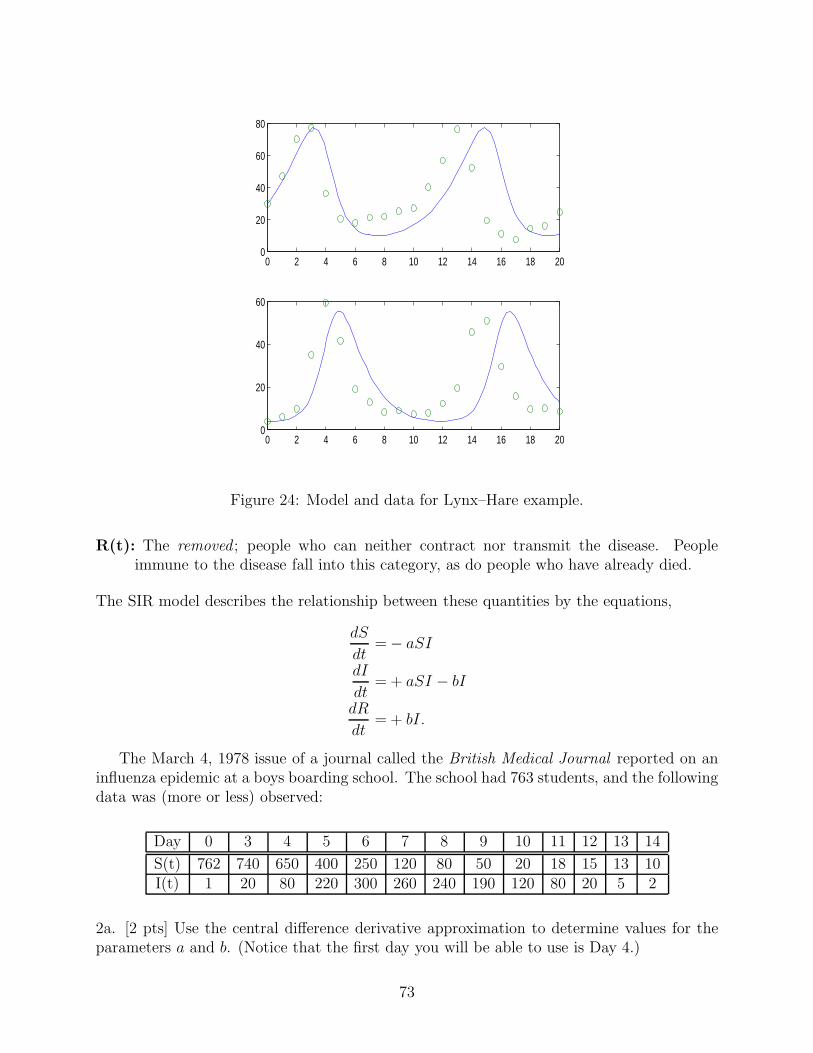
0 2 4 6 8 10 12 14 16 18 200

20

40

60

80

0 2 4 6 8 10 12 14 16 18 200

20

40

60

Figure 24: Model and data for Lynx–Hare example.

R(t): The removed ; people who can neither contract nor transmit the disease. Peopleimmune to the disease fall into this category, as do people who have already died.

The SIR model describes the relationship between these quantities by the equations,

dS

dt= − aSI

dI

dt= + aSI − bI

dR

dt= + bI.

The March 4, 1978 issue of a journal called the British Medical Journal reported on aninfluenza epidemic at a boys boarding school. The school had 763 students, and the followingdata was (more or less) observed:

Day 0 3 4 5 6 7 8 9 10 11 12 13 14

S(t) 762 740 650 400 250 120 80 50 20 18 15 13 10I(t) 1 20 80 220 300 260 240 190 120 80 20 5 2

2a. [2 pts] Use the central difference derivative approximation to determine values for theparameters a and b. (Notice that the first day you will be able to use is Day 4.)

73

2b. [4 pts] Create a stacked plot of your solutions S(t) and I(t) to the SIR model, eachplotted along with the corresponding data.

2c. [2 pts] Compute the error

Error =

√

√

√

√

14∑

d=3

(Smodel(d) − Sdata(d))2.

74

12 Parameter Estimation Directly from ODE, Part 2

12.1 The Direct Method

The two primary advantages of the derivative approximation method toward parameterestimation are that (1) the computation time is typically quite reasonable, and (2) theapproach can be applied with no a priori knowledge about values for the parameters. Theprimary drawback is that the derivative approximations we’re forced to make are often quitecrude. Here, we consider a second method of parameter estimation for ODE for which wecarry out a regression argument directly with the ODE. In general, the method works asfollows. (Warning: The next couple of lines will make a lot more sense once you’ve workedthrough Example 11.1.) Suppose, we have a system of ODE

d~y

dt= f(t, ~y; ~p), ~y ∈ R

n, ~f ∈ Rn,

where ~p is some vector of parameters ~p ∈ Rm, and a collection of k data points: (t1, ~y1),

(t2, ~y2),. . . ,(tk, ~yk). In this notation, for example, the Lotka–Volterra model takes the form

y′1 =p1y1 − p2y1y2

y′2 = − p4y2 + p3y1y2,

where

~y =

(

y1

y2

)

; ~p =

p1

p2

p3

p4

; ~f =

(

f1

f2

)

=

(

p1y1 − p2y1y2

−p4y2 + p3y1y2

)

.

(Notice particularly that a subscript on a vector y indicates a data point, whereas a subscripton a normal y indicates a component.)

We can now determine optimal values for the parameters ~p by minimizing the error,

E(~p) =k

∑

j=1

|~y(tj; ~p) − ~yj|2,

where | · | denotes standard Euclidean vector norm,

|~y| =√

y21 + · · ·+ y2

n.

Example 12.1. Let’s revisit the equations of Example 10.1 with this new method, so we cancompare the final results. First, we write a MATLAB function M-file that contains the Lotka–Volterra model. In system form, we take y1(t) to be prey population and y2(t) to be predatorpopulation. We record the vector of parameters ~p as p = (p(1), p(2), p(3), p(4)) = (a, b, c, r).

function value = lvpe(t,y,p)%LVPE: ODE for example Lotka-Volterra parameter%estimation example. p(1)=a, p(2) = b, p(3) = c, p(4) = r.value=[p(1)*y(1)-p(2)*y(1)*y(2);-p(4)*y(2)+p(3)*y(1)*y(2)];

75

We now develop a MATLAB M-file that takes as input possible values of the parametervector ~p and returns the squared error E(~p). Observe in particular here that in our ode45()statement we have given MATLAB a vector of times (as opposed to the general case, inwhich we give only an initial time and a final time). In this event, MATLAB returns valuesof the dependent variables only at the specified times.

function error = lverr(p)%LVERR: Function defining error function for%example with Lotka-Volterra equations.clear y;lvdata[t,y] = ode45(@lvpe,years,[H(1);L(1)],[],p);value = (y(:,1)-H’).ˆ2+(y(:,2)-L’).ˆ2;%Primes transpose data vectors H and Lerror = sum(value);

Finally, we minimize the function defined in lverr.m with MATLAB’s built-in nonlinearminimizing routine fminsearch(). Observe that we take as our initial guess the values for a,b, c, and r we found through the derivative approximation method. Often, the best way toproceed with parameter estimation is in exactly this way, using the derivative approximationmethod to narrow the search and the direct method to refine it. We arrive at the refinedvalues a = .5486, b = .0283, c = .0264, and r = .8375. The error for the derivativeapproximation error is E = 15528.64, while the error for the direct method is E = 744.79.See Figure 25.

%LVPERUN: MATLAB script M-file to run Lotka-Volterra%parameter estimation example.guess = [.47; .024; .023; .76];[p,error]=fminsearch(@lverr, guess)[t,y]=ode45(@lvpe,[0,20],[30.0; 4.0],[],p);lvdatasubplot(2,1,1)plot(t,y(:,1),years,H,’o’)subplot(2,1,2)plot(t,y(:,2),years,L,’o’)

12.2 Assignments

1. [10 pts] Use our direct method of ODE parameter estimation to obtain a revised set ofparameter values for the SIR epidemic model in Problem 2 of Section 11. Answer parts (2b)and (2c) from Section 11.2, using your new parameter values.

76

0 2 4 6 8 10 12 14 16 18 200

20

40

60

80

0 2 4 6 8 10 12 14 16 18 200

20

40

60

Figure 25: Refined model and data for Lynx–Hare example.

13 Direction Fields

Generally speaking, systems of nonlinear differential equations cannot be solved exactly, andso it’s natural to begin thinking about what can be said about such systems in the absenceof solutions. For systems of two equations a great deal of information can be obtained froma construction called the direction field.

13.1 Plotting Tangent Vectors

Consider the linear system of differential equations

dx

dt= − y; x(0) = 1,

dy

dt=x; y(0) = 0, (16)

for which it is easy to check that (x(t), y(t)) = (cos t, sin t) is a solution. We can plot thissolution pair in the x-y plane with the following MATLAB code, which produces Figure 26.

>>t=linspace(0,2*pi,100);>>x=cos(t);>>y=sin(t);>>plot(x,y)

Let’s consider a point on this curve, say (x, y) = ( 1√2, 1√

2), and determine the slope of the

tangent line at this point. If we regard the top half of the curve as a function y(x), then the

77

−1 −0.8 −0.6 −0.4 −0.2 0 0.2 0.4 0.6 0.8 1−1

−0.8

−0.6

−0.4

−0.2

0

0.2

0.4

0.6

0.8

1

Figure 26: Plot of the curve (cos t, sin t) for t ∈ [0, 2π].

slope is dydx

, which according to the original system of differential equations is

dy

dx= −x

y.

That is to say, the curve has the same slope as the vector (x′(t), y′(t)) = (−y, x). Moreover,the direction of motion corresponds with the direction of this vector. In the case of (x, y) =( 1√

2, 1√

2), this tangent vector is (x′, y′) = (− 1√

2, 1√

2). In order to see this graphically, let’s

add this tangent vector to our plot, setting its tail at the point ( 1√2, 1√

2). MATLAB’s built-in

M-file quiver.m, with usagequiver(x,y,a,b)

places the vector (a, b) at the point (x, y). If the plot in Figure 26 is still active, this arrowcan be added to it with the following MATLAB commands, which create Figure 27.

>>hold on>>quiver(1/sqrt(2),1/sqrt(2),-1/sqrt(2),1/sqrt(2))>>axis equal

Here, the command axis equal must be added while the figure is minimized.Continuing in this manner, we can place vectors at a number of places along the curve,

creating Figure 28.

>>quiver(-1/sqrt(2),1/sqrt(2),-1/sqrt(2),-1/sqrt(2))>>quiver(-1/sqrt(2),-1/sqrt(2),1/sqrt(2),-1/sqrt(2))>>quiver(1/sqrt(2),-1/sqrt(2),1/sqrt(2),1/sqrt(2))>>quiver(0,1,-1,0)

78

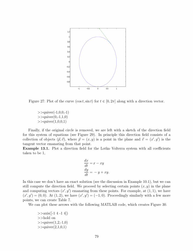
−1 −0.5 0 0.5 1

−0.8

−0.6

−0.4

−0.2

0

0.2

0.4

0.6

0.8

1

1.2

Figure 27: Plot of the curve (cos t, sin t) for t ∈ [0, 2π] along with a direction vector.

>>quiver(-1,0,0,-1)>>quiver(0,-1,1,0)>>quiver(1,0,0,1)

Finally, if the original circle is removed, we are left with a sketch of the direction fieldfor this system of equations (see Figure 29). In principle this direction field consists of acollection of objects (~p,~v), where ~p = (x, y) is a point in the plane and ~v = (x′, y′) is thetangent vector emanating from that point.Example 13.1. Plot a direction field for the Lotka–Volterra system with all coefficientstaken to be 1,

dx

dt= x − xy

dy

dt= − y + xy.

In this case we don’t have an exact solution (see the discussion in Example 10.1), but we canstill compute the direction field. We proceed by selecting certain points (x, y) in the planeand computing vectors (x′, y′) emanating from these points. For example, at (1, 1), we have(x′, y′) = (0, 0). At (1, 2), we have (x′, y′) = (−1, 0). Proceedingly similarly with a few morepoints, we can create Table 7.

We can plot these arrows with the following MATLAB code, which creates Figure 30.

>>axis([-1 4 -1 4])>>hold on>>quiver(1,2,-1,0)>>quiver(2,1,0,1)

79

−1.5 −1 −0.5 0 0.5 1 1.5

−1

−0.5

0

0.5

1

Figure 28: Plot of the curve (cos t, sin t) for t ∈ [0, 2π] along with direction vectors.

(x, y) (x′, y′)

(1, 1) (0, 0)(1, 2) (−1, 0)(2, 1) (0, 1)(1, 0) (1, 0)(0, 1) (0,−1)

Table 7: Direction arrows for the Lotka–Volterra model.

>>quiver(1,0,1,0)>>quiver(0,1,0,-1)

The result is called the direction field for this equation, and though this field does not tellus the solution at each time, it tells us the direction the solution is going from any point. Inother words, integral curves can be sketched in as the curves that are tangent to the vectorsat each point (x, y). Clearly, the more points we place an arrow on, the more information weget. This process is easy to automate, and a nice program that does this has been writtenby John C. Polking, a mathematics professor at Rice University. In order to access this,open an Internet browser and go to http://math.rice.edu/˜dfield. Choose the file pplane7.m(from the M-files for MATLAB 7). From the menu at the top of your browser, choose File,Save Page As, and save this file to your home directory. Now, at the MATLAB prompt,enter pplane7.

In the pplane7 setup menu, replace the default equation with the right-hand sides x−x∗yand −y+x∗y respectively, and change the minimum and maximum values of x and y so that0 ≤ x ≤ 2 and 0 ≤ y ≤ 2. Select proceed from the bottom right corner of the setup menu,and MATLAB will draw a direction field for this equation. If you place your cursor at apoint in the phase plane and select the point by left-clicking the mouse, MATLAB will draw

80

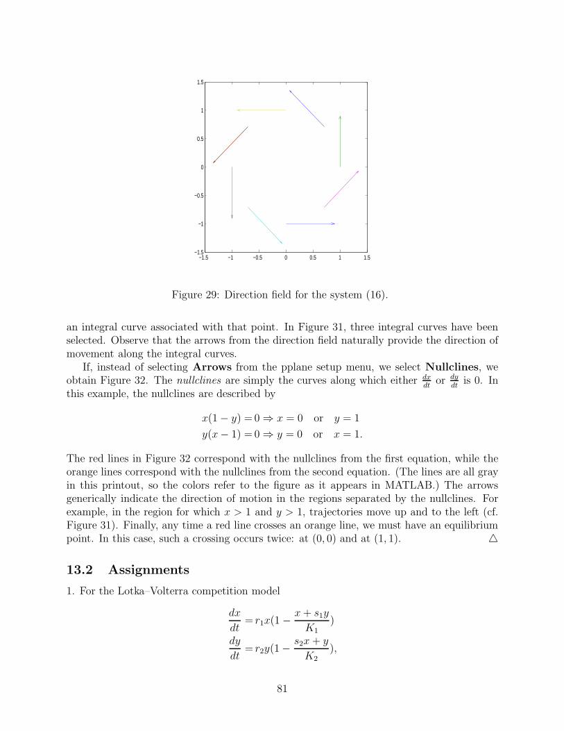
−1.5 −1 −0.5 0 0.5 1 1.5−1.5

−1

−0.5

0

0.5

1

1.5

Figure 29: Direction field for the system (16).

an integral curve associated with that point. In Figure 31, three integral curves have beenselected. Observe that the arrows from the direction field naturally provide the direction ofmovement along the integral curves.

If, instead of selecting Arrows from the pplane setup menu, we select Nullclines, weobtain Figure 32. The nullclines are simply the curves along which either dx

dtor dy

dtis 0. In

this example, the nullclines are described by

x(1 − y) = 0 ⇒ x = 0 or y = 1

y(x− 1) = 0 ⇒ y = 0 or x = 1.

The red lines in Figure 32 correspond with the nullclines from the first equation, while theorange lines correspond with the nullclines from the second equation. (The lines are all grayin this printout, so the colors refer to the figure as it appears in MATLAB.) The arrowsgenerically indicate the direction of motion in the regions separated by the nullclines. Forexample, in the region for which x > 1 and y > 1, trajectories move up and to the left (cf.Figure 31). Finally, any time a red line crosses an orange line, we must have an equilibriumpoint. In this case, such a crossing occurs twice: at (0, 0) and at (1, 1). △

13.2 Assignments

1. For the Lotka–Volterra competition model

dx

dt= r1x(1 − x + s1y

K1)

dy

dt= r2y(1 − s2x + y

K2),

81

−1 −0.5 0 0.5 1 1.5 2 2.5 3 3.5 4−1

−0.5

0

0.5

1

1.5

2

2.5

3

3.5

4

Figure 30: Direction field for the Lotka–Volterra model.

there are four cases of interest: (A) K1 > s1K2, K2 < s2K1, (B) K1 < s1K2, K2 > s2K1,(C) K1 > s1K2, K2 > s2K1, and (D) K1 < s1K2, K2 < s2K1. In this problem we willtake one representative example of each of these cases. For each of the following cases, usethe Nullclines option to find all equilibrium points for the equation (turn in the nullclineplot), and then use the Arrows option to determine whether or not each equilibrium pointis stable or unstable (turn in the direction field plot). Give a physical interpretation of yourresult in each case. In all cases, take r1 = r1 = 1, and K1 = K2 = 1.

(A) [2.5 pts] s1 = 12, s2 = 2.

(B) [2.5 pts] s1 = 2, s2 = 12.

(C) [2.5 pts] s1 = 12, s2 = 1

4.

(D) [2.5 pts] s1 = 4, s2 = 2.

82

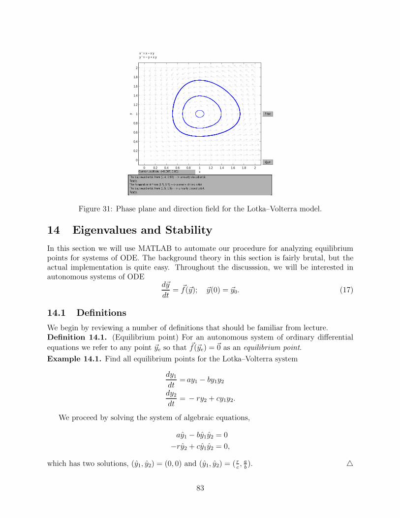
x ’ = x − x y y ’ = − y + x y

0 0.2 0.4 0.6 0.8 1 1.2 1.4 1.6 1.8 2

0

0.2

0.4

0.6

0.8

1

1.2

1.4

1.6

1.8

2

x

y

Figure 31: Phase plane and direction field for the Lotka–Volterra model.

14 Eigenvalues and Stability

In this section we will use MATLAB to automate our procedure for analyzing equilibriumpoints for systems of ODE. The background theory in this section is fairly brutal, but theactual implementation is quite easy. Throughout the discusssion, we will be interested inautonomous systems of ODE

d~y

dt= ~f(~y); ~y(0) = ~y0. (17)

14.1 Definitions

We begin by reviewing a number of definitions that should be familiar from lecture.Definition 14.1. (Equilibrium point) For an autonomous system of ordinary differential

equations we refer to any point ~ye so that ~f(~ye) = ~0 as an equilibrium point.

Example 14.1. Find all equilibrium points for the Lotka–Volterra system

dy1

dt= ay1 − by1y2

dy2

dt= − ry2 + cy1y2.

We proceed by solving the system of algebraic equations,

ay1 − by1y2 = 0

−ry2 + cy1y2 = 0,

which has two solutions, (y1, y2) = (0, 0) and (y1, y2) = ( rc, a

b). △

83

x ’ = x − x y y ’ = − y + x y

0 0.2 0.4 0.6 0.8 1 1.2 1.4 1.6 1.8 2

0

0.2

0.4

0.6

0.8

1

1.2

1.4

1.6

1.8

2

x

y

Figure 32: Nullclines for the Lotka–Volterra equation.

Definition 14.2. (Stability) An equilibrium point ~ye for (17) is called stable if given anyǫ > 0 there exists δ(ǫ) > 0 so that

|~y(0) − ~ye| < δ(ǫ) ⇒ |~y(t) − ~ye| < ǫ for all t > 0.

Definition 14.3. (Asymptotic stability.) An equilibrium point ~ye for (17) is called asymp-totically stable if it is stable and additionally there exists some δ0 > 0 so that

|~y(0) − ~ye| < δ0 ⇒ limt→∞

~y(t) = ~ye.

Definition 14.4. (The Jacobian matrix) For a vector function ~f ∈ Rm of a vector variable

~x ∈ Rn, we define the m × n Jacobian matrix as

D~f =

∂f1

∂x1

∂f1

∂x2

· · · ∂f1

∂xn

∂f2

∂x1

∂f2

∂x2

· · · ∂f2

∂xn

......

......

∂fm

∂x1

∂fm

∂x2

· · · ∂fm

∂xn

. (18)

Definition 14.5. (Differentiability.) We say that a vector function ~f ∈ Rm of n variables

~x ∈ Rn is differentiable at the point ~x0 if the first partial derivatives of all components of ~f

all exist, and if

lim|~h|→0

|~f(~x0 + ~h) − ~f(~x0) − D~f(~x0)~h||~h|

= 0.

Equivalently, ~f(~x) is differentiable at ~x0 if there exists some ~ǫ = ~ǫ(~h) so that

~f(~x0 + ~h) = ~f(~x0) + D~f(~x0)~h + ~ǫ(~h)|~h|,

84

where |~ǫ| → 0 as |~h| → 0. Here, | · | denotes Euclidean norm.

Notice that this definition justifies the notation

~f ′(~y) = D~f(~y).

That is, the Jacobian matrix is the natural structure to define as the derivative of a such avector function.

14.2 Linearization and the Jacobian Matrix

Suppose now that ~ye denotes an equilibrium point for the system (17), and that ~f(~y) isdifferentiable at ~ye (see Definition 13.5). Linearize (17) about ~ye by setting

~y = ~ye + ~z,

where ~z denotes the small perturbation variable (small when ~y is near the equilibrium point).Upon substitution of ~y into (17) we obtain

d

dt(~ye + ~z) = ~f(~ye + ~z).

On the left hand side we haved

dt(~ye + ~z) =

d~z

dt,

whereas on the right hand side we have (by Definition 13.5)

~f(~ye + ~z) = ~f(~ye) + D~f(~ye)~z + ~ǫ(~z)|~z|,

where |~ǫ| → 0 as |~z| → 0. We observe now that ~f(~ye) = ~0 (by definition of an equilibrium

point) and ~ǫ(~z)|~z| is smaller than D~f(~ye)~z (since |~ǫ| → 0 as |~h| → 0.) Therefore we are atleast somewhat justified in taking the approximation

~f(~ye + ~z) ≈ D~f(~ye)~z.

Accordingly, we haved~z

dt≈ D~f(~ye)~z.

This is a linear system of differential equations, and we have seen in class that solutionsto linear systems grow or decay depending upon the signs of the eigenvalues of the linearmatrix. In applying these ideas, we will make use of the following theorem.

Theorem 14.1 (Poincare–Perron). For the ODE system

d~y

dt= ~f(~y),

suppose ~ye denotes an equilibrium point and that ~f is twice continuously differentiable for~y in a neighborhood of ~ye. (I.e., all second order partial derivatives of each component of ~fare continuous.) Then ~ye is stable or unstable as follows:

1. If the eigenvalues of D~f(~ye) all have negative real part, then ~ye is asymptotically stable.

2. If any of the eigenvalues of D~f(~ye) has positive real part then ~ye is unstable.

85

14.3 The Implementation

In practice the analysis of stability of equilibrium points consists of two steps: (1) locatingthe equilibrium points, and (2) finding the eigenvalues of the Jacobian matrix associatedwith each equilibrium point.

Example 14.2. Find all equilibrium points for the Lotka–Volterra competition model

dy1

dt= r1y1(1 −

y1 + s1y2

K1

)

dy2

dt= r2y2(1 −

s2y1 + y2

K2

),

and determine conditions under which each is stable.Worked out by hand, this problem is quite long (see pp. 752–760 in the text), but here

we can let MATLAB do most of the work. We use the M-file stability.m.

%STABILITY: MATLAB script M-file that locates%equilibrium points for the Lotka-Volterra competition%model, computes the Jacobian matrix for each%equilibrium point, and finds the eigenvalues of%each Jacobian matrix.syms y1 y2 r1 K1 s1 r2 K2 s2;y = [y1, y2];f=[r1*y1*(1-(y1+s1*y2)/K1), r2*y2*(1-(s2*y1+y2)/K2)];[ye1 ye2] = solve(f(1),f(2))J = jacobian(f,y)for k=1:length(ye1)y1 = ye1(k)y2 = ye2(k)A = subs(J)lambda = eig(A)end

The only genuinely new command in this file is jacobian, which computes the Jacobianmatrix associated with the vector function ~f with respect to the vector variable ~y. Theimplementation is as follows.

>>stabilityye1 =0K10(-K1+s1*K2)/(-1+s1*s2)ye2 =00

86

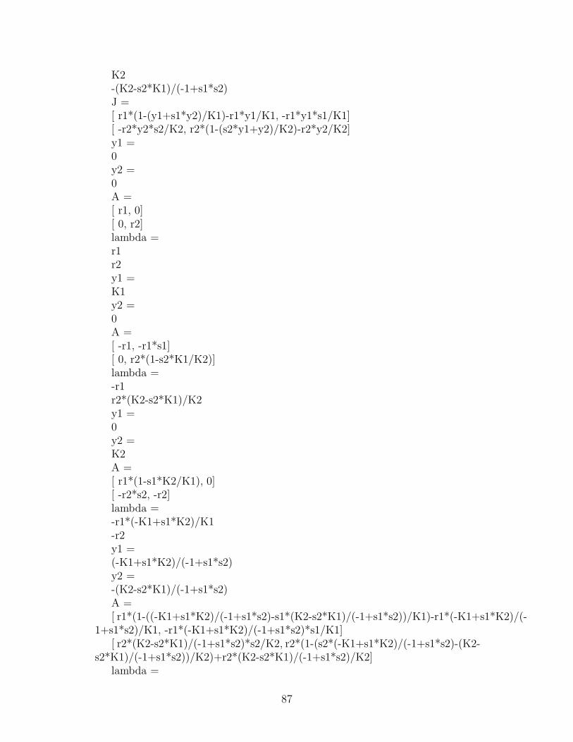
K2-(K2-s2*K1)/(-1+s1*s2)J =[ r1*(1-(y1+s1*y2)/K1)-r1*y1/K1, -r1*y1*s1/K1][ -r2*y2*s2/K2, r2*(1-(s2*y1+y2)/K2)-r2*y2/K2]y1 =0y2 =0A =[ r1, 0][ 0, r2]lambda =r1r2y1 =K1y2 =0A =[ -r1, -r1*s1][ 0, r2*(1-s2*K1/K2)]lambda =-r1r2*(K2-s2*K1)/K2y1 =0y2 =K2A =[ r1*(1-s1*K2/K1), 0][ -r2*s2, -r2]lambda =-r1*(-K1+s1*K2)/K1-r2y1 =(-K1+s1*K2)/(-1+s1*s2)y2 =-(K2-s2*K1)/(-1+s1*s2)A =[ r1*(1-((-K1+s1*K2)/(-1+s1*s2)-s1*(K2-s2*K1)/(-1+s1*s2))/K1)-r1*(-K1+s1*K2)/(-

1+s1*s2)/K1, -r1*(-K1+s1*K2)/(-1+s1*s2)*s1/K1][ r2*(K2-s2*K1)/(-1+s1*s2)*s2/K2, r2*(1-(s2*(-K1+s1*K2)/(-1+s1*s2)-(K2-

s2*K1)/(-1+s1*s2))/K2)+r2*(K2-s2*K1)/(-1+s1*s2)/K2]lambda =

87

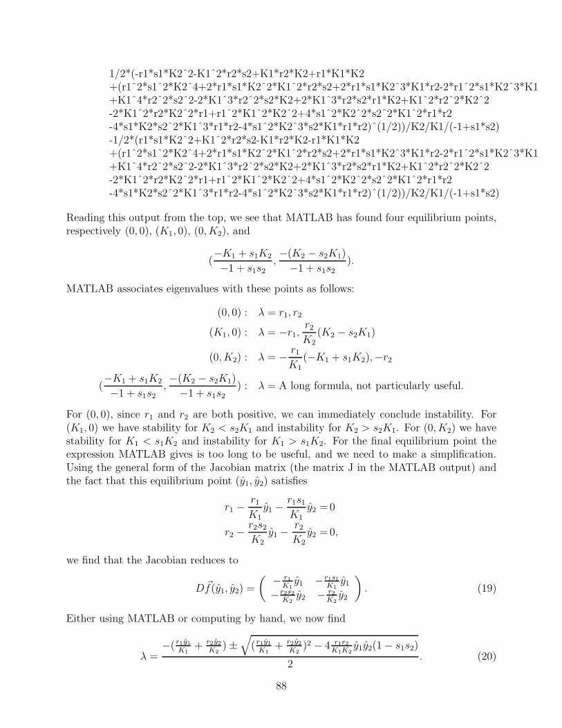
1/2*(-r1*s1*K2ˆ2-K1ˆ2*r2*s2+K1*r2*K2+r1*K1*K2+(r1ˆ2*s1ˆ2*K2ˆ4+2*r1*s1*K2ˆ2*K1ˆ2*r2*s2+2*r1*s1*K2ˆ3*K1*r2-2*r1ˆ2*s1*K2ˆ3*K1+K1ˆ4*r2ˆ2*s2ˆ2-2*K1ˆ3*r2ˆ2*s2*K2+2*K1ˆ3*r2*s2*r1*K2+K1ˆ2*r2ˆ2*K2ˆ2-2*K1ˆ2*r2*K2ˆ2*r1+r1ˆ2*K1ˆ2*K2ˆ2+4*s1ˆ2*K2ˆ2*s2ˆ2*K1ˆ2*r1*r2-4*s1*K2*s2ˆ2*K1ˆ3*r1*r2-4*s1ˆ2*K2ˆ3*s2*K1*r1*r2)ˆ(1/2))/K2/K1/(-1+s1*s2)-1/2*(r1*s1*K2ˆ2+K1ˆ2*r2*s2-K1*r2*K2-r1*K1*K2+(r1ˆ2*s1ˆ2*K2ˆ4+2*r1*s1*K2ˆ2*K1ˆ2*r2*s2+2*r1*s1*K2ˆ3*K1*r2-2*r1ˆ2*s1*K2ˆ3*K1+K1ˆ4*r2ˆ2*s2ˆ2-2*K1ˆ3*r2ˆ2*s2*K2+2*K1ˆ3*r2*s2*r1*K2+K1ˆ2*r2ˆ2*K2ˆ2-2*K1ˆ2*r2*K2ˆ2*r1+r1ˆ2*K1ˆ2*K2ˆ2+4*s1ˆ2*K2ˆ2*s2ˆ2*K1ˆ2*r1*r2-4*s1*K2*s2ˆ2*K1ˆ3*r1*r2-4*s1ˆ2*K2ˆ3*s2*K1*r1*r2)ˆ(1/2))/K2/K1/(-1+s1*s2)

Reading this output from the top, we see that MATLAB has found four equilibrium points,respectively (0, 0), (K1, 0), (0, K2), and

(−K1 + s1K2

−1 + s1s2

,−(K2 − s2K1)

−1 + s1s2

).

MATLAB associates eigenvalues with these points as follows:

(0, 0) : λ = r1, r2

(K1, 0) : λ = −r1,r2

K2(K2 − s2K1)

(0, K2) : λ = − r1

K1

(−K1 + s1K2),−r2

(−K1 + s1K2

−1 + s1s2,−(K2 − s2K1)

−1 + s1s2) : λ = A long formula, not particularly useful.

For (0, 0), since r1 and r2 are both positive, we can immediately conclude instability. For(K1, 0) we have stability for K2 < s2K1 and instability for K2 > s2K1. For (0, K2) we havestability for K1 < s1K2 and instability for K1 > s1K2. For the final equilibrium point theexpression MATLAB gives is too long to be useful, and we need to make a simplification.Using the general form of the Jacobian matrix (the matrix J in the MATLAB output) andthe fact that this equilibrium point (y1, y2) satisfies

r1 −r1

K1

y1 −r1s1

K1

y2 =0

r2 −r2s2

K2y1 −

r2

K2y2 =0,

we find that the Jacobian reduces to

D~f(y1, y2) =

( − r1

K1

y1 −r1s1

K1

y1

−r2s2

K2

y2 − r2

K2

y2

)

. (19)

Either using MATLAB or computing by hand, we now find

λ =−( r1y1

K1

+ r2y2

K2

) ±√

( r1y1

K1

+ r2y2

K2

)2 − 4 r1r2

K1K2

y1y2(1 − s1s2)

2. (20)

88

We now see that the equilibrium point is stable if (1−s1s2) > 0 and unstable if (1−s1s2) < 0.△

In many cases we know specific parameter values for our model, and this serves to simplifythe analysis considerably.

Example 14.3. Given the parameter values r1 = r2 = K1 = K2 = 1, s1 = 12, and s2 = 1

4,

find all equilibrium points for the Lotka–Volterra competition model and determine whetheror not each is stable.

Of course we could proceed simply by plugging these values into the expressions fromExample 13.2, but let’s instead edit our M-file so that the calculation is automated.

%STABILITY2: MATLAB script M-file that locates%equilibrium points for the Lotka-Volterra competition%model, computes the Jacobian matrix for each%equilibrium point, and finds the eigenvalues of%each Jacobian matrix. Parameter values are chosen%as r1=r2=K1=K2=1, s1=.5, s2=.25.syms y1 y2;y = [y1, y2];f=[y1*(1-(y1+y2/2)), y2*(1-(y1/4+y2))];[ye1 ye2] = solve(f(1),f(2))J = jacobian(f,y)for k=1:length(ye1)y1 = eval(ye1(k))y2 = eval(ye2(k))A = subs(J)lambda = eig(A)end

Note in particular that the parameters are no longer defined symbolically, but rather appeardirectly in the equations. Also, eval commands have been added to make y1 and y2 numerical.We find:

>>stability2ye1 =0104/7ye2 =0016/7J =[ 1-2*y1-1/2*y2, -1/2*y1]

89

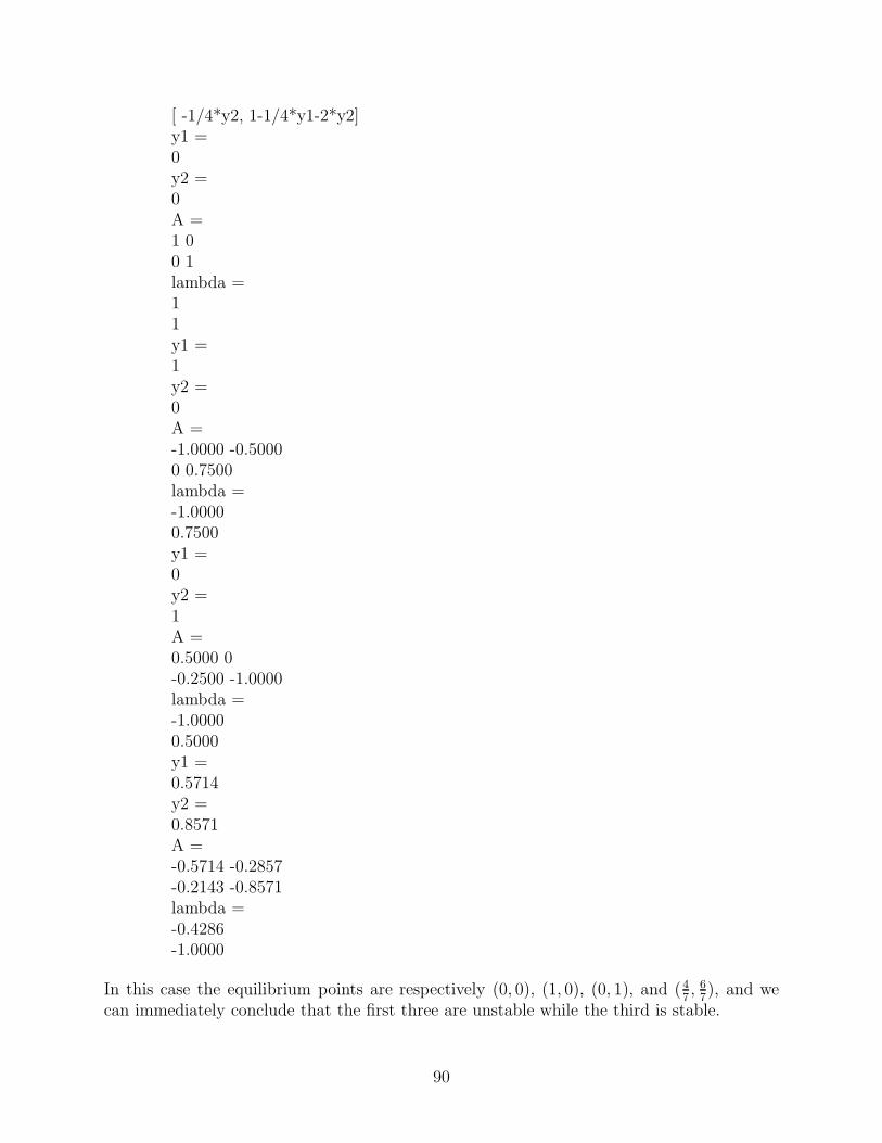
[ -1/4*y2, 1-1/4*y1-2*y2]y1 =0y2 =0A =1 00 1lambda =11y1 =1y2 =0A =-1.0000 -0.50000 0.7500lambda =-1.00000.7500y1 =0y2 =1A =0.5000 0-0.2500 -1.0000lambda =-1.00000.5000y1 =0.5714y2 =0.8571A =-0.5714 -0.2857-0.2143 -0.8571lambda =-0.4286-1.0000

In this case the equilibrium points are respectively (0, 0), (1, 0), (0, 1), and (47, 6

7), and we

can immediately conclude that the first three are unstable while the third is stable.

90

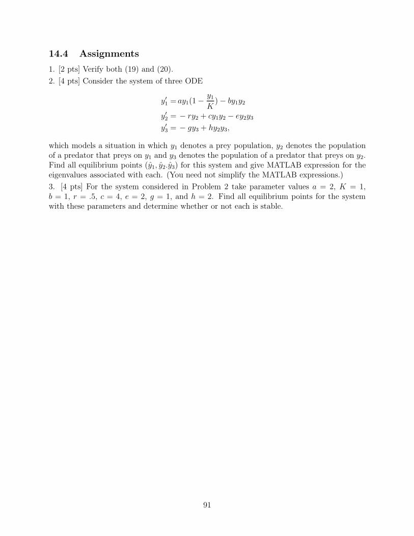
14.4 Assignments

1. [2 pts] Verify both (19) and (20).

2. [4 pts] Consider the system of three ODE

y′1 = ay1(1 −

y1

K) − by1y2

y′2 = − ry2 + cy1y2 − ey2y3

y′3 = − gy3 + hy2y3,

which models a situation in which y1 denotes a prey population, y2 denotes the populationof a predator that preys on y1 and y3 denotes the population of a predator that preys on y2.Find all equilibrium points (y1, y2.y3) for this system and give MATLAB expression for theeigenvalues associated with each. (You need not simplify the MATLAB expressions.)

3. [4 pts] For the system considered in Problem 2 take parameter values a = 2, K = 1,b = 1, r = .5, c = 4, e = 2, g = 1, and h = 2. Find all equilibrium points for the systemwith these parameters and determine whether or not each is stable.

91