1

MATLAB Code Description

7 November 2013 Computational approach to characterize causative factors and molecular indicators of chronic wound inflammation by Sridevi Nagaraja, Anders Wallqvist, Jaques Reifman, and Alexander Y. Mitrophanov

Correspondence about modeling- and software-related technical questions to Sridevi Nagaraja: snagaraja@bhsai.org

2

CONTENTS Overview ........................................................................................................................................... 3

System Requirements ....................................................................................................................... 3

MATLAB Code Description ............................................................................................................ 3

Acute Inflammation Model ............................................................................................................... 4

Local Sensitivity Analysis ................................................................................................................ 8

Extended Sensitivity Analysis (randomized parameter sets) ............................................................ 9

3

Overview The MATLAB code for the inflammation model was developed at the Biotechnology High Performance Computing Software Applications Institute (BHSAI), Ft. Detrick, Maryland, to study the triggers of chronic inflammation as well as to identify the sensitive molecular mediators of chronic inflammation. The software currently implements a set of ordinary differential equations (ODEs) and a delay differential equation (DDE) to simulate acute and chronic inflammatory responses. Local sensitivity analysis was implemented to identify the triggers and sensitive indicators of chronic inflammation. The inputs for the acute inflammation model as well as the sensitivity analyses are embedded in the code. The user can directly change parameter values inside some of the provided MATLAB files. The System Requirements Section contains the details about the computer system that we used to develop and run the code. The rest of this document provides information about using the code for the three different types of analysis described in the paper (inflammation time course modeling, local sensitivity analysis for the default parameter set, and local sensitivity analysis for 10,000 random parameter sets). System Requirements We used the following software and hardware components: Software • Operating System: Windows 7 Enterprise (64-bit operating system) • MATLAB version 7.14.0.739 (R2012a) (64-bit operating system) • MATLAB Statistics Toolbox, Version 8.0 (R2012a) • Microsoft Excel 2010 for plotting the figures in the paper Hardware • Intel® Core(TM) 2 Duo CPU E8400 @ 3.00 GHz and 4.00 GB RAM • Disk space: 3–4 GB is recommended for a typical installation For extended sensitivity analysis, we used two server computers with the following specifications: • CPU: 2x Intel Xeon X5650 (6 cores @ 2.66 GHz) • RAM: 24 GB @ 1333 MHz • Disk space: 4x 300 GB @ 10,000 RPM MATLAB Code Description The code was developed in MATLAB 2012a. It includes the following files:

4

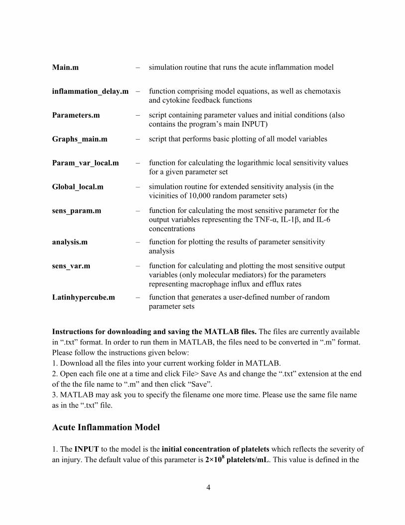
Main.m – simulation routine that runs the acute inflammation model

inflammation_delay.m – function comprising model equations, as well as chemotaxis and cytokine feedback functions

Parameters.m – script containing parameter values and initial conditions (also contains the program’s main INPUT)

Graphs_main.m – script that performs basic plotting of all model variables

Param_var_local.m – function for calculating the logarithmic local sensitivity values for a given parameter set

Global_local.m – simulation routine for extended sensitivity analysis (in the vicinities of 10,000 random parameter sets)

sens_param.m – function for calculating the most sensitive parameter for the output variables representing the TNF-α, IL-1β, and IL-6 concentrations

analysis.m – function for plotting the results of parameter sensitivity analysis

sens_var.m – function for calculating and plotting the most sensitive output variables (only molecular mediators) for the parameters representing macrophage influx and efflux rates

Latinhypercube.m – function that generates a user-defined number of random parameter sets

Instructions for downloading and saving the MATLAB files. The files are currently available in “.txt” format. In order to run them in MATLAB, the files need to be converted in “.m” format. Please follow the instructions given below: 1. Download all the files into your current working folder in MATLAB. 2. Open each file one at a time and click File> Save As and change the “.txt” extension at the end of the the file name to “.m” and then click “Save”. 3. MATLAB may ask you to specify the filename one more time. Please use the same file name as in the “.txt” file. Acute Inflammation Model 1. The INPUT to the model is the initial concentration of platelets which reflects the severity of an injury. The default value of this parameter is 2×108 platelets/mL. This value is defined in the

5

“Parameters.m” file under “Initial conditions”. To increase or decrease the severity of an injury, increase or decrease the value of the parameter “P_init” in this file. Note: Any additional simulation of interest, e.g., chronic inflammation induced by a 5-fold higher macrophage influx rate or by an alteration in the production rate of a specific cytokine, will need to be initiated by changing the respective parameter in the “Parameters.m” file. 2. To run the model, open “Main.m” and click the “Run” icon or type “Main” in the MATLAB command window. 3. After the routine is executed, the kinetic curves of all the model variables will be displayed as outputs in 5 separate figures, as shown below. Figure 1: Kinetics of total neutrophil and macrophage concentrations Figure 2: Kinetics of individual neutrophil and macrophage phenotype concentrations Figure 3: Kinetics of growth factor and platelet concentrations Figure 4: Kinetics of TNF-α, IL-1β, IL-6, and IL-10 concentrations Figure 5: Kinetics of CXCL8, IL-12, MIP-1α, and MIP-2 concentrations

6

7

8

4. These output figures show the raw output values calculated by the model. The raw values of all output variables, as well as simulation time points, are stored in the output variable “g” in the MATLAB workspace. Note: The raw values of all output variables of the model were imported into Microsoft (MS) EXCEL, normalized, and plotted along with normalized experimental data, as shown in Figs. 3 and 5 in the paper. Supplemental Fig. S2 in the paper shows the results plotted in Figure 2 of this simulation without additional processing. Note: Chronic inflammation simulations shown in Fig. 5 of the paper were performed by executing the file “Main.m” after increasing the macrophage influx rate parameter “kM_in” by 5-fold of its default value in the “Parameters.m” file. Local Sensitivity Analysis Simulation: To calculate the local sensitivity values in the vicinity of the default parameter set, open the file “Main.m” and uncomment the last two lines under “Local sensitivity analysis” (lines 34−35). Then, click on the “Run” icon or type “Main” in the MATLAB command window. Output: The raw sensitivity values for all output variables at 21 simulated time points for each of the 69 main model parameters are stored in the output variable “Gsen_local” (a structure of size 1×73, where each element represents the simulation for a particular parameter variation) in the MATLAB workspace. Note: The code contains definitions for 73 parameters, some of which were excluded in the current version of the model and assigned zero values. Therefore, all the sensitivity vectors have a size of 73. Plotting: Fig. 4A in the paper shows values from the first element of the output variable “O_b_l”, which extracts and saves from the sensitivity matrix “Gsen_local”, the identifying numbers of the parameters that demonstrate the highest sensitivity to TNF-α, IL-1β, and IL-6 concentrations for all time points in the simulation.

Note: For a complete list of the parameter identifying numbers, check the file “Parameters.m”. Each parameter is assigned an identifying number shown in the comment next to its initialization.

9

Extended Sensitivity Analysis (randomized parameter sets) Simulation: To calculate sensitivity values for a number of random parameter sets, follow the instructions given below: 1. Open “Global_local.m”.

2. Change the value of the parameter “iter” to choose the number of randomly generated parameter sets (default value used in the paper: 10,000). 3. Change the value of the parameter “rangefactor” to increase or decrease the uniform distribution sampling range for the extended sensitivity analysis [default value used in the paper: 2, i.e, the parameter values in the generated sets are chosen randomly from a 4-fold range (2-fold higher and 2-fold lower than default value)]. Note: To perform the sensitivity analysis on one parameter set using one node takes approximately 5 minutes. Therefore, to compute the sensitivity values for 10,000 parameter sets, we used 12 parallel nodes, and the simulation took approximately 16 hours to complete. The user is recommended to start with smaller values of “iter” (e.g., 50 or 100). If using parallel processing, replace the “for” command in “Global_local.m”, line 30, by “parfor” and specify the number of nodes that will be used in “matlabpool” command right before using “parfor”. 4. Click on the “Run” icon or type “Global_local” in the MATLAB command window. Output: The raw sensitivities for all the model outputs with respect to all the 69 parameters at 21 time points for the 10,000 random parameter sets are stored in the output variable “Gsen” in the MATLAB workspace. The size of this file is ~2.3 GB. The sensitivity values of the output variables TNF-α, IL-1β, and IL-6 with respect to all the model parameters across all the 10,000 parameter sets are extracted from “Gsen”, ranked in descending order, and stored in the output variable “O_val”. The identifying numbers assigned to the parameters corresponding to the respective sensitivity values are stored in the output variable “O_b” in the MATLAB workspace. The kinetic curves for all output variables for each of the randomly generated parameter sets are stored in the variable “Ymain_d” in the MATLAB workspace. Plotting inflammation triggers: To plot the results for the most important parameters/mechanisms, follow the instructions given below: 1. Uncomment the three lines under the “Plotting the critical triggers of chronic inflammation” section (lines 37−39) in the file “Global_local.m”.

10

2. Specify the number of most important parameter/mechanisms you want to plot by changing the parameter “rnk”. (Default value: 3, which plots the identifying numbers of the parameters with highest, second-highest, and third-highest sensitivities for TNF-α, IL-1β, and IL-6 at every simulated time point.) 3. Copy and paste the three lines into MATLAB command window. The output will generate “rnk” number of figures. A sample figure for the model parameters with the highest sensitivity (Rank = 1) for TNF-α, IL-1β, and IL-6, respectively, is shown below:

4. The figures show the identifying number of parameter whose sensitivity had a given rank (highest, second highest …) for the largest fraction of the 10,000 randomly generated parameter sets for each of the selected output variables (in our case: TNF-α, IL-1β, and IL-6) and each of the simulated time points (gray bars, left-hand y-axis). The actual value of this largest fraction (denoted in the plots as “Frequency”) is displayed on the right-hand y-axis (shown in red). Note: These raw sensitivity values were then imported into MS EXCEL and used to calculate the robustness of each parameter as the percentage of the 10,000 parameter sets for which this parameters’ sensitivity ranked as most sensitive for TNF-α, IL-1β, and IL-6 at 3 different simulated time points (shown as the pie charts in Fig.4B of the paper).

11

5. To visualize the most sensitive parameters for another output variable (other than TNF-α, IL-1β, and IL-6), change the output variable identifying numbers in the vector “P_param” in the file “Global_local.m” and copy/paste the three lines (37−39) into the MATLAB command window. (For a complete list of output variable identifying numbers, check the file “inflammation_delay.m”. Each output variable is assigned an identifying number shown in the comment next to its initialization). Use only three output variable identifying numbers at a time. Plotting sensitive molecular mediators: To analyze and plot the results for the most sensitive molecular indicators, follow the instructions given below: 1. Uncomment the lines under “Plotting the most sensitive molecular mediators of chronic inflammation” section (lines 43−45) in the file “Global_local.m” and comment back the previous section “Plotting the critical trigger of chronic inflammation” (lines 37−39). 2. Specify the number of most sensitive molecular indicators you want to plot by changing the parameter “rnk”. (Default value: 3; which plots the top three molecular mediator outputs most sensitive to parameter #7 (i.e., macrophage influx rate) and parameter #10 (i.e., macrophage efflux rate). 3. Copy and paste the three lines into the MATLAB command window. The output will comprise “rnk” number of figures. A sample figure for the model output variables with highest sensitivity (Rank =1) is shown below. 4. The figures show the identifying number of model output variable whose sensitivity had a given rank (highest, second-highest, …) for the largest fraction of the 10,000 randomly generated parameter sets for each of the selected parameters (in our case: macrophage influx and efflux rates denoted in the MATLAB code as kM_in and kd_M) and each of the simulated time points (gray bars, left-hand y-axis). The actual value of this largest fraction (denoted in the plots as “Frequency”) is displayed on the right-hand y-axis (shown in blue). Note: These raw sensitivity values were then imported into MS EXCEL and used to calculate the robustness of each parameter as the percentage of the 10,000 parameter sets for which this output variables’ sensitivity ranked as highest, second-highest, and third-highest for kM_in and kd_M at 4 different simulated time points (shown as bar graphs in Figs. 6 and 7 of the paper).

12

5. To visualize the most sensitive molecular mediators for another parameter/mechanism (other than kM_in and kd_M), change the parameter identifying numbers in the vector “P_var” in the file “Global_local.m” and copy/paste the three lines (43−45) in to the MATLAB command window. (For a complete list of parameter identifying numbers, check the file “Parameters.m”. Each parameter is assigned an identifying number shown in the comment next to its initialization). Use only two parameters identifying numbers at a time.