1 23

Boletín de la Sociedad MatemáticaMexicanaThird Series ISSN 1405-213X Bol. Soc. Mat. Mex.DOI 10.1007/s40590-015-0054-x

Conditions for the Schur stability ofsegments of polynomials of the same degree

Baltazar Aguirre-Hernández, RicardoGarcía-Sosa, Horacio Leyva, Julio Solís-Daun & Francisco A. Carrillo

1 23

Your article is protected by copyright and

all rights are held exclusively by Sociedad

Matemática Mexicana. This e-offprint is for

personal use only and shall not be self-

archived in electronic repositories. If you wish

to self-archive your article, please use the

accepted manuscript version for posting on

your own website. You may further deposit

the accepted manuscript version in any

repository, provided it is only made publicly

available 12 months after official publication

or later and provided acknowledgement is

given to the original source of publication

and a link is inserted to the published article

on Springer's website. The link must be

accompanied by the following text: "The final

publication is available at link.springer.com”.

Bol. Soc. Mat. Mex.DOI 10.1007/s40590-015-0054-x

ORIGINAL ARTICLE

Conditions for the Schur stabilityof segments of polynomials of the same degree

Baltazar Aguirre-Hernández · Ricardo García-Sosa ·Horacio Leyva · Julio Solís-Daun · Francisco A. Carrillo

Received: 20 December 2013 / Accepted: 5 February 2015© Sociedad Matemática Mexicana 2015

Abstract One of the most interesting problems in the robustness analysis of systems isthe investigation of conditions that guarantee the stability of segments of polynomials.In this paper, given two polynomials P1(z) and P2(z) of the same degree, we giveconditions on the polynomial H(z) = zn[P1(z)P2(

1z ) − P1(

1z )P2(z)] such that the

Schur stability of the segment [P1, P2] is implied by the Schur stability of both P1(z)and P2(z).

Keywords Roots of polynomials · Schur polynomials · Segments of Schurpolynomials · Stability · Schur stability

Mathematics Subject Classification 93C05 · 93D09 · 93D20

B. Aguirre-Hernández (B) · J. Solís-DaunDivisión de Ciencias Básicas e Ingeniería, Departamento de Matemáticas, Universidad AutónomaMetropolitana–Iztapalapa, Av. San Rafael Atlixco 186, Col. Vicentina, Del. Iztapalapa, A.P. 55-534,C.P. 09340 Mexico, D.F., Mexicoe-mail: bahe@xanum.uam.mx

J. Solís-Daune-mail: jesd@xanum.uam.mx

R. García-SosaUPIICSA–SEPI, Instituto Politécnico Nacional, Av. Té. 950, C.P. 08400 Mexico, D.F., Mexicoe-mail: frgarcia@ipn.mx

H. Leyva · F. A. CarrilloDepartamento de Matemáticas, Universidad de Sonora, Blvd. Luis Encinas y Rosales s/n, Col. Centro,Hermosillo, Sonora, Mexicoe-mail: hleyva@gauss.mat.uson.mx

F. A. Carrilloe-mail: carrillo@gauss.mat.uson.mx

Author's personal copy

B. Aguirre-Hernández et al.

1 Introduction

It is known that the set of Hurwitz polynomials as well as the set of Schur polynomialsis non-convex. Consequently, it is useful to find methods for checking if the seg-ment of polynomials Pλ(z) = λP0(z) + (1 − λ)P1(z) is stable for all λ ∈ [0, 1].Another motivation for knowing the stability of segments of polynomials is thefact that the stability of an entire polytope of polynomials is implied by the sta-bility of its edges (see [9]). Different techniques have been reported to verify thestability of segments of polynomials (see [1–4,13,15,16,22,31,41]). On the otherhand, the concept of convex direction is very related with the study of the stabil-ity of segments of polynomials: a polynomial δ0(t) is called a convex direction ifthe Hurwitz or Schur stability of the segment λδ1(z) + (1 − λ)[δ1(z) − δ0(z)], forλ ∈ [0, 1], is guaranteed whenever the endpoints δ1(t) and δ1(t) − δ0(t) are sta-ble. Results about convex directions and special polynomials which can be iden-tified as convex directions can be found in [19,20,23,25,37–39]. The conditionsgiven by the Convex Direction Theorems presented in [8,10,39] are frequencydependent. When we have frequency-independent conditions on δ0(t), it is saidthat we have a vertex theorem or vertex lemma. The results about Vertex Theo-rems were obtained by different researchers (see [11,12,25,29,33,36]). However,the concept of convex direction may be restrictive in some robust stability prob-lems: a polynomial δ0(t) may ensure the stability of λδ1(t) + (1 − λ)[δ1(t) −δ0(t)], λ ∈ [0, 1], for a given polynomial δ1(t), without being a convex direc-tion (see [24,43,45]). In such a case, we say that δ0(t) is a local convex direc-tion.

Other properties and related questions about Hurwitz and Schur polynomials canbe found in [5–7,21,26,27,32]. With respect to families of Hurwitz and Schur poly-nomials, interesting questions were posed in [14,17,18,28,30,34,35,40,42,44]

In this paper, we give frequency-independent conditions to guarantee the Schurstability of a segment of polynomials. Such frequency-independent conditions are

given on the polynomial H(z) = zn[

P1(z)P2(1z ) − P1(

1z )P2(z)

](not on P0(z) =

P1(z) − P2(z)). Consequently, we could say that our result is a vertex-like theorem.Specifically, we study even-degree polynomials of the form q(z) = z2m + q1z2m−1 +q2z2m−2+· · ·+qm−1zm+1+qm zm +qm−1zm−1+· · ·+q1z+1, and we give conditionsto have all their roots on the unit circle. Then, we apply the result to attain sufficientconditions for the Schur stability of a segment of polynomials of the same degree.

The paper is organized as follows. In Sect. 2, we present the main theorems aboutthe roots of a kind of even-degree polynomials and we apply the main results to studythe Schur stability of a segment of polynomials. Then, in Sect. 3, we present theconclusions.

2 Main results

In the first subsection, we provide necessary and sufficient conditions for a kind ofeven-degree polynomials to have their roots on the unit circle. Then, in the second

Author's personal copy

Conditions for Schur stability

subsection, we establish a method for deciding whether a segment of polynomials isSchur stable.

2.1 Even-degree polynomials with roots on the unit circle

In this subsection, we give necessary and sufficient conditions for a kind of even-degree polynomials to have all their roots on the unit circle. First, we establish theresult for polynomials with degree equal to 2.

Lemma 1 The polynomial f (z) = z2 + az + 1 has its roots on the unit circle if andonly if |a| ≤ 2.

Proof If z1 and z2 are roots of f (z) and |z1| = 1 and |z2| = 1, we have that a =−z1 − z2 and consequently |a| = |z1 + z2| ≤ |z1| + |z2| = 1 + 1 = 2. Now, wesuppose that |a| ≤ 2.

(i) If z1, z2 ∈ R then a = −z1 − z2, z1z2 = 1 then z2 = 1z1

and a = −z1 − 1z1

,

consequently |a| ≤ 2 ⇔∣∣∣∣

z21+1z1

∣∣∣∣ ≤ 2 ⇔ ∣∣z21 + 1

∣∣ ≤ 2 |z1| ⇔ |z1|2 − 2 |z1| + 1 ≤0 ⇔ (|z1| − 1)2 ≤ 0 ⇔ |z1| = 1.

(ii) If z1 = x + iy, z2 = x − iy then 2 ≥ |a| = 2 |x |, and hence |x | ≤ 1 and1 = z1z2 = x2 + y2, that is |z1| = |z2| = 1.

��Example 1 Consider the polynomial f (z) = z2 + 1

3 z + 1. Then,∣∣ 1

3

∣∣ < 2, and the

roots of f (z) are z = −16 ± 1

6

√35i , so that

∣∣∣−16 ± 1

6

√35i

∣∣∣ = 1.

Now, consider the real polynomial q(z) = z2m + q1z2m−1 + q2z2m−2 + · · · +qm−1zm+1 + qm zm + qm−1zm−1 + · · · + q1z + 1.

For a complex number α, we define the matrix Am−1(α) ∈ M(m−1)×(m−1) as

Am−1(α) =

⎛⎜⎜⎜⎜⎜⎜⎜⎜⎜⎜⎝

1 0 0 . . . 0 0 0 0 0α 1 0 . . . 0 0 0 0 01 α 1 . . . 0 0 0 0 00 1 α . . . 0 0 0 0 00 0 1 . . . 0 0 0 0 0· · · · · · · · ·0 0 0 . . . 0 1 α 1 00 0 0 . . . 0 0 1 α 1

⎞⎟⎟⎟⎟⎟⎟⎟⎟⎟⎟⎠

, (1)

and let r(α) be given by the following (m − 1)-vector

⎛⎜⎜⎜⎝

r1(α)

r2(α)...

rm−1(α)

⎞⎟⎟⎟⎠= A−1

m−1(α)

⎛⎜⎜⎜⎜⎜⎜⎝

q1 − α

q2 − 1q3. . .

qm−2qm−1

⎞⎟⎟⎟⎟⎟⎟⎠

. (2)

Author's personal copy

B. Aguirre-Hernández et al.

where A−1m−1(α) can be written as

A−1m−1(α) =

⎡⎢⎢⎢⎢⎢⎢⎢⎢⎢⎢⎢⎢⎢⎢⎢⎣

1 0 0 · · · 0 0 0 0 0 0−α 1 0 · · · 0 0 0 0 0 0

B2(α) −α 1 · · · 0 0 0 0 0 0B3(α) B2(α) −α · · · 0 0 0 0 0 0B4(α) B3(α) B2(α) · · · 0 0 0 0 0 0B5(α) B4(α) B3(α) · · · 0 0 0 0 0 0B6(α) B5(α) B4(α) · · · 0 0 0 0 0 0

......

... · · · ......

......

......

Bm−3(α) Bm−4(α) Bm−5(α) · · · B4(α) B3(α) B2(α) −α 1 0Bm−2(α) Bm−3(α) Bm−4(α) · · · B5(α) B4(α) B3(α) B2(α) −α 1

⎤⎥⎥⎥⎥⎥⎥⎥⎥⎥⎥⎥⎥⎥⎥⎥⎦

(3)

with

B2(α) = α2 − 1,

B3(α) = −α3 + 2 α,

B4(α) = α4 − 3 α2 + 1,

B5(α) = −α5 + 4 α3 − 3 α,

B6(α) = α6 − 5 α4 + 6 α2 − 1,

...

Bm−3(α) = (−1)m−2(αm−3 − · · · ),Bm−2(α) = (−1)m−1(αm−2 − · · · ).

where Bp(α) is a p-degree polynomial for p = 0, 1, . . . , n − 2 (see the proof in theAppendix). Define the m-degree polynomial

hm(α) = αrm−1(α) + 2rm−2(α) − qm, (4)

where rm−1 and rm−2 satisfy Eqs. (7) and (8) of the Appendix, that is, hm is definedin an explicit form in terms of the elements of A−1

m−1(α). Then, the following resultshold.

Lemma 2 Consider the real polynomial q(z) = z2m + q1z2m−1 + q2z2m−2 + · · · +qm−1zm+1 +qm zm +qm−1zm−1 +· · ·+q1z +1. We have that there exists a (2m −2)-degree polynomial with the same form that q(z), that is r(z) = z2m−2+r1z2m−3+· · ·+rm−2zm +rm−1zm−1+rm−2zm−2+· · ·+r1z+1, such that

(z2 + αz + 1

)r(z) = q(z),

if and only if (2) is satisfied and hm(α) = 0

Proof Straightforward calculations show us that there exist α and r(z) = z2m−2 +r1z2m−3 + · · · + rm−2zm + rm−1zm−1 + rm−2zm−2 + · · · + r1z + 1, such that (z2 +αz + 1)r(z) = q(z) if and only if (2) is satisfied and 2rm−2 +αrm−1 = qm if and onlyif (2) is satisfied and hm(α) = 0 [see (4)]. ��

Author's personal copy

Conditions for Schur stability

Theorem 1 All the roots of hm(α) have magnitude less than or equal to 2 if and onlyif all the roots of q(z) have magnitude 1.

Proof The idea of the proof is the following: if all the roots of q(z) have magnitude1 then q(z) can be written as

q(z) = (z2 + α1z + 1)(z2 + α2z + 1) . . . (z2 + αm z + 1)

where the α′i s are the roots of hm(α).

Suppose that α1, . . . , αm are the roots of hm(α) and |αi | ≤ 2 for every i = 1, . . . , m,then z2 + αi z + 1 has roots on the unit circle by Lemma 1. Moreover, z2 + αi z + 1is factor of q(z) for every i = 1, . . . , m, by Lemma 2. Consequently, all the roots ofq(z) are on the unit circle. Conversely, if we suppose that the real polynomial q(z) hasall its roots on the unit circle, then for each pair of roots z0 and z0 on the unit circle,we have q(z) = (z − z0)(z − z0)u(z), that is q(z) = (z2 − [z0 + z0]z + z0z0)u(z).Clearly, z0z0 = 1. We define α1 = −(z0 + z0). Again, by Lemma 1, we have that|α1| ≤ 2. Then, q(z) can be written as q(z) = (z2 +α1z +1)r(z). Following with thisprocedure, we have that q(z) can be written as q(z) = (z2+α1z+1) . . . (z2+αm z+1)

with |αi | ≤ 2 for i = 1, . . . , m since the α′i s are the roots of hm(α) by Lemma 2. ��

Remark 1 The importance of the previous result will be appreciated in the next sub-section, where we illustrate how it can be used to obtain the stability of segment ofpolynomials.

2.2 Applications: Segments of Schur polynomials

A segment of polynomials [P1, P2] is not necessarily Schur stable in spite of the factthat P1 and P2 are Schur stable, for instance P1(z) = z3 + 1.5z2 + 1.2z + 0.5 andP2(z) = z3 − 1.2z2 + 1.1z − 0.4 are Schur stable, however, λP1(z) + (1 − λ)P2(z) isnot Schur stable for all λ ∈ [0, 1]. In fact, λP1(z) + (1 − λ)p2(z) is not Schur stablefor λ = 0.7755 (see [10, p. 88]).

In this subsection, we give conditions for the Schur stability of a segment of poly-nomials. Such conditions are obtained from Theorem 1.

In fact, consider the Schur polynomials with real coefficients P1(z) = anzn +an−1zn−1 +· · ·+a1z +a0 and P2(z) = bnzn +bn−1zn−1 +· · ·+b1z +b0; and define

H(z) = zn[

P1(z)P2

(1

z

)− P1

(1

z

)P2(z)

], (5)

The function H(z) has been used in previous works: (The equality H(z)zn = 0 is one of

the three conditions in the Segment Lemma (see pages 83, 84 in [10])).It can be seen that H(z) can be rewritten as

H(z) = cnz2n + cn−1z2n−1 + cn−2z2n−2 + · · · + c1zn+1 − c1zn−1 − c2zn−2

− · · · − cn−1z − cn,

Author's personal copy

B. Aguirre-Hernández et al.

where

cn = anb0 − a0bn

cn−1 = an−1b0 + anb1 − a1bn − a0bn−1

cn−2 = an−2b0 + an−1b1 + anb2 − a2bn − a1bn−1 −−a0bn−2

· · ·c1 = a1b0 + a2b1 + · · · + anbn−1 −

− an−1bn − · · · − a1b2 − a0b1.

Moreover, it can be checked that H(z) = cn(z2 − 1)T (z), where T (z) = z2n−2 +d1z2n−3 +d2z2n−4 +· · ·+dn−3zn+1 +dn−2zn +dn−1zn−1 +dn−2zn−2 +dn−3zn−3 +· · ·+d2z2+d1z+1, with d1 = cn−1

cn, d2 = cn−2+cn

cn, d3 = cn−3+cn−1

cn, d4 = cn−4+cn−2+cn

cn,

…, dn−1 = c1+c3+c5+···cn

.Consider An−2(α) ∈ M(n−2)×(n−2) as in (1) (taking m = n − 1) and e(α) as

follows

e(α) =

⎛⎜⎜⎜⎜⎜⎝

e1(α)

e2(α)...

en−3(α)

en−2(α)

⎞⎟⎟⎟⎟⎟⎠

= A−1n−2(α)

⎛⎜⎜⎜⎜⎜⎜⎝

d1 − α

d2 − 1d3. . .

dn−3dn−2

⎞⎟⎟⎟⎟⎟⎟⎠

.

If we denote by F and G the following (n − 1)-degree polynomials, F(α) =αen−2(α) + 2en−3(α) − dn−1 and G(α) = αn−1 F

( 2α

), then we have the follow-

ing result.

Theorem 2 Consider the n-degree Schur polynomials with real coefficients P1 andP2. If the following conditions

(a) G(α) is a Schur polynomial,(b) P1(1)

P2(1)> 0, and

(c) P1(−1)P2(−1)

> 0,

are satisfied, then the segment [P1(z), P2(z)] is Schur stable.

Proof By the Segment Lemma ([10,41,44]), we have that [P1(z), P2(z)] is a segmentof Schur polynomial if there is not z0 with |z0| = 1, such that H(z0) = 0 (see[4]) and P1(z0)

P2(z0)≤ 0, (In the Appendix, we have included the Segment Lemma). If

G(α) = αn F( 2α) is Schur, then the roots of F(α) have magnitude greater than two,

whence by Theorem 1, T (z) has no roots with magnitudes equal to 1, then z = 1 andz = −1 are all of the roots of H(z) = cn(z2 − 1)T (z), so that they have magnitudeequal to one. Therefore, based on Conditions (a), (b) and (c), and the Segment Lemma,we obtain that [P1(z), P2(z)] is Schur stable.

Author's personal copy

Conditions for Schur stability

Remark 2 There exist other works where the Schur stability of segments of polynomi-als has been studied. For example, in Theorem 12 of [22], it is pointed out that the Schurstability of a segment of n-degree polynomials can be verified if two (n −1)× (n −1)

matrices are non-zero innerwise. An advantage of our approach is that we need toverify that the (n −1)-degree polynomial G(α) is Schur stable which implies to checkthat two (n − 2) × (n − 2) matrices are positive innerwise. Moreover, the matricesconsidered in [22] depend on a parameter.

In the case of Theorem 11.17 in [1], the Schur stability of a segment of polynomialsis verified checking that an (n−1)×(n−1) matrix has no non-positive real eigenvalues,which has a similar complexity than our approach since we need that the (n−1)-degreepolynomial G(α) has n − 1 roots with magnitude less than 1. On the other hand, itcan be said that the Theorem 2 of this paper is a version of the Segment Lemma in[10], in terms of the coefficients, in the sense that the results in this paper allow us toshow that the Schur stability of a segment with extremes P1 and P2 can be verifiedchecking the Schur stability of a third polynomial G(α).

In relation with the three aforementioned methods, the disadvantage of our approachis that the results in [1,10,22] are necessary and sufficient conditions, whereas ourresult is a sufficient condition. Now, we present two examples to illustrate the resultpresented in Theorem 2.

Example 2 Consider P1(z) = (z + 12 )4 = z4 + 2z3 + 1.5z2 + 0.5z + 0.0625, a4 = 1,

a3 = 2, a2 = 1.5, a1 = 0.5, a0 = 0.0625, P2(z) = z4 + 1.7839z3 + 1.4269z2 +0.4857z + 0.0626, b4 = 1, b3 = 1.7839, b2 = 1.4269, b1 = 0.4857, b0 = 0.0626,

where

c4 = a4b0 − a0b4 = 0.0001

c3 = a3b0 + a4b1 − a1b4 − a0b3 = −0.0006

c2 = a2b0 + a3b1 + a4b2 − a2b4 − a1b3 −−a0b2 = 0.011

c1 = a1b0 + a2b1 + a3b2 + a4b3 −− a3b4 − a2b3 − a1b2 − a0b1 = −0.0222

d1 = c3

c4= −0.0006

0.0001= −6

d2 = c2 + c4

c4= 0.0111

0.0001= 111

d3 = c1 + c3

c4= −0.0228

0.0001= −228,

On the other hand,

(e1(α)

e2(α)

)= A−1

2 (α)

(d1 − α

d2 − 1

)=

(1 0

−α 1

) (−6 − α

110

)

=( −6 − α

α2 + 6α + 110

),

Author's personal copy

B. Aguirre-Hernández et al.

then

F(α) = α[e2(α)] + 2e1(α) − d3

= α[α2 + 6α + 110] + 2(−6 − α) − (−228)

= α3 + 6α2 + 108α + 216

Finally, as G(α) = α3 F( 2α) then G(α) = 216α3 +216α2 +24α+8. The zeroes of

G(α) are α = −0.9231, α = −0.03845 ± 0.19658i . Then, G(α) is Schur. Therefore,the segment [P1(z), P2(z)] is Schur stable.

Example 3 Consider P1(z) = z5 + 0.5 z4 + 0.1 z3 + 0.01 z2 + 0.005 z + 0.00001,a5 = 1, a4 = 0.5, a3 = 0.1, a2 = 0.01, a1 = 0.005, a0 = 0.00001, P2(z) =10, 000 z5 + 5565.59 z4 + 662.62 z3 + 209.97 z2 + 33.506 z + 1.1, b5 = 10, 000,b4 = 5565.59, b3 = 662.62, b2 = 209.97, b1 = 33.506, b0 = 1.1,

c5 = a5b0 − a0b5 = 1,

c4 = a4b0 + a5b1 − a0b4 − a1b5 = −16,

c3 = a3b0 + a4b1 + a5b2 − a0b3 − a1b4 − a2b5 = 99,

c2 = a2b0 + a3b1 + a4b2 + a5b3 − a3b5 − a2b4 − a1b3 − a0b2 = −288,

c1 = a1b0 + a2b1 + a3b2 + a4b3 + a5b4 − a4b5 − a3b4 − a2b3 − a1b2 − a0b1 = 354,

d1 = c4

c5= −16

1= −16,

d2 = c3 + c5

c5= 99 + 1

1= 100,

d3 = c2 + c4

c5= −288 − 16

1= −304,

d4 = c1 + c3 + c5

c5= 354 + 99 + 1

1= 454.

On the other hand,

⎛⎝

e1(α)

e2(α)

e3(α)

⎞⎠ = A−1

3 (α)

⎛⎝

d1 − α

d2 − 1d3

⎞⎠ =

⎛⎝

1 0 0−α 1 0

α2 − 1 −α 1

⎞⎠

⎛⎝

−16 − α

100 − 1−304

⎞⎠

=⎛⎝

−16 − α

α2 + 16α + 99−α3 − 16α2 − 98α − 288

⎞⎠ ,

then

F(α) = αe3(α) + 2e2(α) − d4

= α(−α3 − 16α2 − 98α − 288

)+ 2

(α2 + 16α + 99

)− 454

= −α4 − 16α3 − 96α2 − 256α − 256

Author's personal copy

Conditions for Schur stability

G(α) = α4 F

(2

α

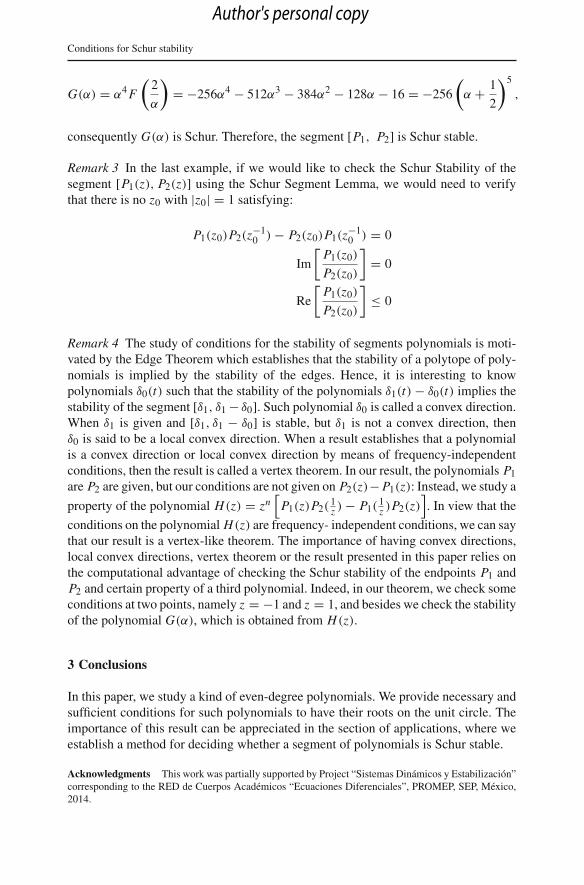
)= −256α4 − 512α3 − 384α2 − 128α − 16 = −256

(α + 1

2

)5

,

consequently G(α) is Schur. Therefore, the segment [P1, P2] is Schur stable.

Remark 3 In the last example, if we would like to check the Schur Stability of thesegment [P1(z), P2(z)] using the Schur Segment Lemma, we would need to verifythat there is no z0 with |z0| = 1 satisfying:

P1(z0)P2(z−10 ) − P2(z0)P1(z

−10 ) = 0

Im

[P1(z0)

P2(z0)

]= 0

Re

[P1(z0)

P2(z0)

]≤ 0

Remark 4 The study of conditions for the stability of segments polynomials is moti-vated by the Edge Theorem which establishes that the stability of a polytope of poly-nomials is implied by the stability of the edges. Hence, it is interesting to knowpolynomials δ0(t) such that the stability of the polynomials δ1(t) − δ0(t) implies thestability of the segment [δ1, δ1 − δ0]. Such polynomial δ0 is called a convex direction.When δ1 is given and [δ1, δ1 − δ0] is stable, but δ1 is not a convex direction, thenδ0 is said to be a local convex direction. When a result establishes that a polynomialis a convex direction or local convex direction by means of frequency-independentconditions, then the result is called a vertex theorem. In our result, the polynomials P1are P2 are given, but our conditions are not given on P2(z)− P1(z): Instead, we study a

property of the polynomial H(z) = zn[

P1(z)P2(1z ) − P1(

1z )P2(z)

]. In view that the

conditions on the polynomial H(z) are frequency- independent conditions, we can saythat our result is a vertex-like theorem. The importance of having convex directions,local convex directions, vertex theorem or the result presented in this paper relies onthe computational advantage of checking the Schur stability of the endpoints P1 andP2 and certain property of a third polynomial. Indeed, in our theorem, we check someconditions at two points, namely z = −1 and z = 1, and besides we check the stabilityof the polynomial G(α), which is obtained from H(z).

3 Conclusions

In this paper, we study a kind of even-degree polynomials. We provide necessary andsufficient conditions for such polynomials to have their roots on the unit circle. Theimportance of this result can be appreciated in the section of applications, where weestablish a method for deciding whether a segment of polynomials is Schur stable.

Acknowledgments This work was partially supported by Project “Sistemas Dinámicos y Estabilización”corresponding to the RED de Cuerpos Académicos “Ecuaciones Diferenciales”, PROMEP, SEP, México,2014.

Author's personal copy

B. Aguirre-Hernández et al.

Appendix

Proposition 1 Consider the matrix Am−1(α) ∈ M(m−1)×(m−1) defined by (1) whereα is a complex number. Then, A−1

m−1(α) has the form indicated in (3), where Bp(α) isa p-degree polynomial for p = 0, 1, . . . , m − 2

Proof Induction.For n = 3, 4, 5 we have that

A−12 (α) =

[1 0

−α 1

]

A−13 (α) =

⎡⎣

1 0 0−α 1 0

α2 − 1 −α 1

⎤⎦

A−14 (α) =

⎡⎢⎢⎣

1 0 0 0−α 1 0 0

α2 − 1 −α 1 0−α3 + 2α α2 − 1 −α 1

⎤⎥⎥⎦

Suppose that the proposition is valid for m − 1 and now we will prove it for m.Analyzing A−1

m , we first note that A−1m must be a lower triangular matrix and the

element in the row i and the column j is the same that the element in the row i + 1and column j + 1.

Then, the m × m matrix A−1m (α) has the following form

A−1m (α) =

⎡⎢⎢⎢⎢⎢⎢⎢⎢⎢⎣

B0(α) 0 0 · · · 0 0 0 0 0 0 0B1(α) B0(α) 0 · · · 0 0 0 0 0 0 0B2(α) B1(α) B0(α) · · · 0 0 0 0 0 0 0B3(α) B2(α) B1(α) · · · 0 0 0 0 0 0 0

.

.

....

.

.

. · · ·...

.

.

....

.

.

....

.

.

....

Bm−2(α) Bm−3(α) Bm−4(α) · · · B5(α) B4(α) B3(α) B2(α) B1(α) B0(α) 0Bm−1(α) Bm−2(α) Bm−3(α) · · · B6(α) B5(α) B4(α) B3(α) B2(α) B1(α) B0(α)

⎤⎥⎥⎥⎥⎥⎥⎥⎥⎥⎦

Note that, the following (n − 1) × (n − 1) submatrix

⎡⎢⎢⎢⎢⎢⎢⎢⎣

B0(α) 0 0 · · · 0 0 0 0 0 0B1(α) B0(α) 0 · · · 0 0 0 0 0 0B2(α) B1(α) B0(α) · · · 0 0 0 0 0 0B3(α) B2(α) B1(α) · · · 0 0 0 0 0 0

......

... · · · ......

......

......

Bm−2(α) Bm−3(α) Bm−4(α) · · · B5(α) B4(α) B3(α) B2(α) B1(α) B0(α)

⎤⎥⎥⎥⎥⎥⎥⎥⎦

is the inverse matrix of the (n − 1) × (n − 1) matrix Am−1(α)

Author's personal copy

Conditions for Schur stability

Consequently, (By Inductive Hypothesis) Bp(α) is a p-degree polynomial for p =0, 1, . . . , m − 2. Now, via a straightforward calculation, it can be verified that

A−1m (α) =

(A−1

m−1(α) 0m−1

− (0 . . . 0 1 α

)A−1

m (α) 1

)(6)

Therefore,

Bm−1(α) = − (0 . . . 1 α

)⎛⎜⎜⎝

B0(α)

B1(α)

· · ·Bm−2(α)

⎞⎟⎟⎠

Hence, Bm−1(α) is a m − 1-degree polynomial since Bp is p-degree polynomial forp = 0, 1, . . . , m − 2 ��Proposition 2 The number rm−1(α) and rm−2(α) satisfy

rm−1(α) = − (0 . . . 0 1 α

)m−2 A−1

m−2(α)

⎛⎜⎜⎜⎜⎝

q1 − α

q2 − 1q3· · ·

qm−2

⎞⎟⎟⎟⎟⎠

+ qm−1 (7)

rm−2(α) = − (0 . . . 0 1 α

)m−3 A−1

m−3(α)

⎛⎜⎜⎜⎜⎝

q1 − α

q2 − 1q3· · ·

qm−3

⎞⎟⎟⎟⎟⎠

+ qm−2 (8)

where(

0 . . . 0 1 α)

m−2 ∈ Rm−2,(

0 . . . 0 1 α)

m−3 ∈ Rm−3

Proof By Eq. (5), we can write that

⎛⎜⎜⎜⎜⎝

r1(α)

r2(α)

· · ·rm−2(α)

rm−1(α)

⎞⎟⎟⎟⎟⎠

=(

A−1m−2(α) 0m−2

− (0 · · · 0 1 α)m−2 A−1m−2(α) 1

)

⎛⎜⎜⎜⎜⎜⎜⎝

q1 − α

q2 − 1q3· · ·

qm−2qm−1

⎞⎟⎟⎟⎟⎟⎟⎠

=⎛⎜⎝

A−1m−3(α) 0m−3 0m−3

− (0 . . . 0 1 α

)m−3 A−1

m−3(α) 1 0− (

0 . . . 0 1 α)

m−2 A−1m−2(α) 1

⎞⎟⎠

⎛⎜⎜⎜⎜⎜⎜⎝

q1 − α

q2 − 1q3· · ·

qm−2qm−1

⎞⎟⎟⎟⎟⎟⎟⎠

whence the result is obtained. ��

Author's personal copy

B. Aguirre-Hernández et al.

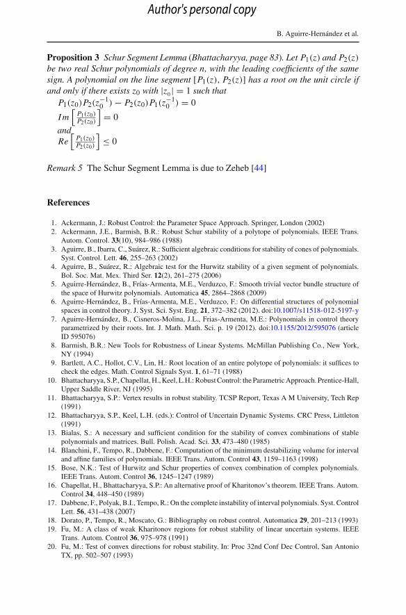
Proposition 3 Schur Segment Lemma (Bhattacharyya, page 83). Let P1(z) and P2(z)be two real Schur polynomials of degree n, with the leading coefficients of the samesign. A polynomial on the line segment [P1(z), P2(z)] has a root on the unit circle ifand only if there exists z0 with |z0 | = 1 such that

P1(z0)P2(z−10 ) − P2(z0)P1(z

−10 ) = 0

I m[

P1(z0)P2(z0)

]= 0

andRe

[P1(z0)P2(z0)

]≤ 0

Remark 5 The Schur Segment Lemma is due to Zeheb [44]

References

1. Ackermann, J.: Robust Control: the Parameter Space Approach. Springer, London (2002)2. Ackermann, J.E., Barmish, B.R.: Robust Schur stability of a polytope of polynomials. IEEE Trans.

Autom. Control. 33(10), 984–986 (1988)3. Aguirre, B., Ibarra, C., Suárez, R.: Sufficient algebraic conditions for stability of cones of polynomials.

Syst. Control. Lett. 46, 255–263 (2002)4. Aguirre, B., Suárez, R.: Algebraic test for the Hurwitz stability of a given segment of polynomials.

Bol. Soc. Mat. Mex. Third Ser. 12(2), 261–275 (2006)5. Aguirre-Hernández, B., Frías-Armenta, M.E., Verduzco, F.: Smooth trivial vector bundle structure of

the space of Hurwitz polynomials. Automatica 45, 2864–2868 (2009)6. Aguirre-Hernández, B., Frías-Armenta, M.E., Verduzco, F.: On differential structures of polynomial

spaces in control theory. J. Syst. Sci. Syst. Eng. 21, 372–382 (2012). doi:10.1007/s11518-012-5197-y7. Aguirre-Hernández, B., Cisneros-Molina, J.L., Frias-Armenta, M.E.: Polynomials in control theory

parametrized by their roots. Int. J. Math. Math. Sci. p. 19 (2012). doi:10.1155/2012/595076 (articleID 595076)

8. Barmish, B.R.: New Tools for Robustness of Linear Systems. McMillan Publishing Co., New York,NY (1994)

9. Bartlett, A.C., Hollot, C.V., Lin, H.: Root location of an entire polytope of polynomials: it suffices tocheck the edges. Math. Control Signals Syst. 1, 61–71 (1988)

10. Bhattacharyya, S.P., Chapellat, H., Keel, L.H.: Robust Control: the Parametric Approach. Prentice-Hall,Upper Saddle River, NJ (1995)

11. Bhattacharyya, S.P.: Vertex results in robust stability. TCSP Report, Texas A M University, Tech Rep(1991)

12. Bhattacharyya, S.P., Keel, L.H. (eds.): Control of Uncertain Dynamic Systems. CRC Press, Littleton(1991)

13. Bialas, S.: A necessary and sufficient condition for the stability of convex combinations of stablepolynomials and matrices. Bull. Polish. Acad. Sci. 33, 473–480 (1985)

14. Blanchini, F., Tempo, R., Dabbene, F.: Computation of the minimum destabilizing volume for intervaland affine families of polynomials. IEEE Trans. Autom. Control 43, 1159–1163 (1998)

15. Bose, N.K.: Test of Hurwitz and Schur properties of convex combination of complex polynomials.IEEE Trans. Autom. Control 36, 1245–1247 (1989)

16. Chapellat, H., Bhattacharyya, S.P.: An alternative proof of Kharitonov’s theorem. IEEE Trans. Autom.Control 34, 448–450 (1989)

17. Dabbene, F., Polyak, B.I., Tempo, R.: On the complete instability of interval polynomials. Syst. ControlLett. 56, 431–438 (2007)

18. Dorato, P., Tempo, R., Moscato, G.: Bibliography on robust control. Automatica 29, 201–213 (1993)19. Fu, M.: A class of weak Kharitonov regions for robust stability of linear uncertain systems. IEEE

Trans. Autom. Control 36, 975–978 (1991)20. Fu, M.: Test of convex directions for robust stability. In: Proc 32nd Conf Dec Control, San Antonio

TX, pp. 502–507 (1993)

Author's personal copy

Conditions for Schur stability

21. García, R., Aguirre, B., Suárez, R.: Stabilization of linear sampled-data systems by a time-delayfeedback control. Math. Prob. Eng. p. 15 (2008). doi:10.1155/2008/270518 (article ID 270518)

22. Góra, M.: Stability of the convex combination of polynomials. Control Cybern. 36(2), 425 (2007)23. Hinrichsen, D., Kharitonov, V.L.: On convex directions for stable polynomials. Report 309, Institute

of Dynamic Systems, University of Bremen, pp. 1–22 (1994)24. Hinrichsen, D., Kharitonov, V.L.: Stability of polynomials with conic uncertainty. Math. Control Sig-

nals Syst. 8, 97–117 (1995)25. Hollot, C.V., Yang, F.: Robust stabilization of interval plants using lead or lag compensators. Syst.

Control Lett. 14, 9–12 (1996)26. Jury, E.I.: Sampled-Data Control systems. Wiley, New York (1977)27. Jury, E.I.: Inners and Stability of Dynamic Systems. Krieger Pub. Co., Malabar, Florida (1982)28. Kale Amit, A., Tits, A.I.: On Kharitonov’s theorem without invariant degree assumption. Automatica

36, 1075–1076 (2000)29. Kang, HI.: Extreme point results for robustness of control systems. Ph.D. thesis, Department Electrical

& Computer Engng, University of Wisconsin, USA (1992)30. Kharitonov, V.L.: Asymptotic stability of an equilibrium position of a family of systems of linear

differential equations. Dif Urav 14, 2086–2088 (1978). English translation in Diff Eqs, 14: 1483–1485(1979)

31. López-Renteria, J.A., Aguirre-Hernández, B., Verduzco, F.: The boundary crossing theorem and themaximal stability interval. Math. Prob. Eng. p. 13 (2011). doi:10.1155/2011/12340

32. Loredo-Villalobos, C.A., Aguirre-Hernández, B.: Necessary conditions for Hadamard factorizationsof Hurwitz polynomials. Automatica 47, 1409–1413 (2011)

33. Mansour, M., Kraus, F.S.: Argument conditions for Hurwitz and Schur stable polynomials and therobust stability problem. Tech Rep, ETH, Zurich (1990)

34. Nurges, A.: New stability conditions via reflection coefficients of polynomials. IEEE Trans. Autom.Control 50(9), 1354–1360 (2005)

35. Nurges, A.: Robust pole assignment via reflection coefficients of polynomials. Automatica 42(7),1223–1230 (2006)

36. Petersen, I.R.: A new extension to Kharitonov’s theorem. In: Proc IEEE Conf Dec Control, Los AngelesCA, pp. 2070–2075 (1987)

37. Petersen, I.R.: A class of stability regions for which a Kharitonov like theorem holds. IEEE Trans.Autom. Control 34, 1111–1115 (1989)

38. Rantzer, A.: Hurwitz testing sets for parallel polytopes of polynomials. Syst. Control Lett. 15, 99–104(1990)

39. Rantzer, A.: Stability conditions for polytopes of polynomials. IEEE Trans. Autom. Control 37, 79–89(1992)

40. Tempo, R.: A dual resul to kharitonov theorem. IEEE Trans. Autom. Control 35, 195–198 (1990)41. Tin, M.A.: Discrete time robust control systems under structured perturbations: Stability manifolds and

extremal properties. Master’s thesis, Departament of Electrical Engineering, Texas A&M University,College Station, Texas, USA (1992)

42. Willems, J.C., Tempo, R.: The Kharitonov theorem with degrre drop. IEEE Trans. Autom. Control 44,2218–2220 (1999)

43. Zeheb, E.: Necessary and sufficient conditions for root clustering of polytope of polynomials in asimply connected domain. IEEE Trans. Autom. Control 34, 986–990 (1989)

44. Zeheb, E.: Necessary and sufficient conditions for the robust stability of a continuous system: thecontinuous dependency case illustrated by multilinear dependence. IEEE Trans. Circ. Syst. 37, 47–53(1990)

45. Zeheb, E.: On the characterization and formation of local convex directions. In: Jeltsch, R., Mansour,M. (eds) Stability theory, Birkhäuser, Basel, Switzerland pp. 173–180 (1996)

Author's personal copy