mathematisches forschungsinstitut oberwolfach · pimentel (2004) shows that the competition...

Mathematisches Forschungsinstitut Oberwolfach

Report No. 43/2004

Large Scale Stochastic Dynamics

Organised byClaudio Landim (Rio de Janeiro)

Stefano Olla (Paris)

Herbert Spohn (Munchen)

August 29th–September 4th, 2004

Introduction by the Organisers

“Large Scale Stochastic Dynamics” is at the crossroad of probability theory andstatistical physics. One central theme of statistical physics is the emergent be-havior resulting from the interaction of many identical components, the paradigmbeing a fluid or a gas. On the atomistic scale they consist of a huge number ofidentical molecules. Their motion is governed by Newton’s equations of classi-cal mechanics (ignoring quantum effects). The emergent description, valid onlyfor particular initial states and on a sufficiently coarse space-time scale, are thecompressible Navier-Stokes equations of fluid dynamics. Roland Dobrushin (1929–1995) and Frank Spitzer (1926–1992) had the vision that in the context of stochas-tic dynamics with many identical components the issue of emergent behavior isboth mathematically challenging and important in modelling applications. Thelatter judgement turned out to be more than true. Stochastic algorithms, such askinetic Monte Carlo, importance sampling, Monte Carlo Markov chains, Glauberdynamics, and others, are daily practice. Their mathematical vision has evolvedover the past twenty years into a rich, multifaceted research program. Our work-shop is like a snap-shot of the current activities. A partial list of topics reads

• hydrodynamic limit for multi-component stochastic lattice gases• steady state large deviations for driven systems• random walks in random environments• directed polymer in a random potential, spin glasses• statics and dynamics of interfaces• glassy dynamics

2230 Oberwolfach Report 43/2004

We had 49 participants from 11 countries, mostly probabilists, but also expertsfrom partial differential equations and statistical physics. They all enjoyed tremen-dously the unique and stimulating atmosphere at the Mathematische Forschungsin-stitut Oberwolfach and hope to return some day.

Claudio Landim,Stefano Olla,Herbert Spohn.

Large Scale Stochastic Dynamics 2231

Workshop: Large Scale Stochastic Dynamics

Table of Contents

Pablo A. Ferrari (joint with Leandro P. R. Pimentel)Competition interfaces in last-passage percolation and second classparticles . . . . . . . . . . . . . . . . . . . . . . . . . . . . . . . . . . . . . . . . . . . . . . . . . . . . . . . . . 2233

M.C. Cranston and T. MountfordLyapunov Exponent for the Parabolic Anderson Model in Rd . . . . . . . . . . . 2235

Philippe Carmona (joint with Yueyun Hu)Universality in Sherrington-Kirkpatrick’s Spin Glass Model . . . . . . . . . . . . . 2236

Cedric BernardinKawasaki dynamics at critical temperature . . . . . . . . . . . . . . . . . . . . . . . . . . . 2238

Joel L. Lebowitz (joint with O. Costin, T. Kuna and E. R. Speer)On the Realizability of Point Processes with SpecifiedOne and Two Particle Densities . . . . . . . . . . . . . . . . . . . . . . . . . . . . . . . . . . . . 2241

Cristina Toninelli (joint with G.Biroli and D.S.Fisher)Stochastic lattice gases with dynamical constraints and glassy dynamics . . 2244

Dmitry IoffeLocal Functional of Phase Separation Lines . . . . . . . . . . . . . . . . . . . . . . . . . . . 2248

Thierry Bodineau (joint with Bernard Derrida)Current fluctuations in non-equilibrium diffusive systems . . . . . . . . . . . . . . . 2251

Francis Comets (joint with Nobuo Yoshida)The directed polymer in random environment is diffusive at weak disorder 2253

Nobuo Yoshida (joint with Francis Comets)Brownian Directed Polymers in Random Environment . . . . . . . . . . . . . . . . . 2256

Ofer Zeitouni (joint with Alain-Sol Sznitman)Diffusive behavior of isotropic diffusions in random environment . . . . . . . . 2257

Gunter M. Schutz (joint with R.D. Willmann and S. Großkinsky)Spontaneous symmetry breaking in a driven two-species lattice gas . . . . . . . 2257

Jozsef Fritz (joint with Balint Toth)Hyperbolic scaling problems: The method of compensated compactness . . . . 2260

Balint Toth and Benedek ValkoPerturbation of equilibria: a hydrodynamic limit . . . . . . . . . . . . . . . . . . . . . . . 2263

Ellen Saada (joint with C. Bahadoran, H. Guiol, K. Ravishankar)Euler hydrodynamics of one-dimensional attractive particle systems . . . . . . 2266


Sunder SethuramanDiffusive limit for a tagged particle in asymmetric zero-range . . . . . . . . . . . 2268

M. Mourragui (joint with Enza Orlandi)Large deviations from a macroscopic scaling limit for particle systemswith Kac interaction and random potential . . . . . . . . . . . . . . . . . . . . . . . . . . . 2270

Katalin Nagy (joint with Jozsef Fritz and Stefano Olla)Equilibrium Fluctuations for a System of Harmonic Oscillators withConservative Noise . . . . . . . . . . . . . . . . . . . . . . . . . . . . . . . . . . . . . . . . . . . . . . . . 2272

Marton BalazsRandom walking shocks in interacting particle systems . . . . . . . . . . . . . . . . . 2275

Stefan Großkinsky (joint with G.M. Schutz and H. Spohn)Condensation in the Zero Range Process . . . . . . . . . . . . . . . . . . . . . . . . . . . . . 2277

Milton Jara (joint with Claudio Landim)Nonequilibrium CLT for a tagged particle in symmetric simple exclusion . 2279

Glauco Valle (joint with Claudio Landim)A microscopic interpretation of Stefan’s melting and freezing problem . . . . 2280

G. Jona-Lasinio (joint with L. Bertini, A. De Sole, D. Gabrielli, C. Landim)Macroscopic current fluctuations in stochastic lattice gases . . . . . . . . . . . . . 2282

Camille Enaud (joint with Bernard Derrida)Large deviation functional and fluctuations of density in the WASEP . . . . 2284

Erwin Bolthausen (joint with Nicola Kistler)On a non-hierarchical version of the Generalized Random Energy Model . 2286

Christophe BahadoranHydrodynamics of asymmetric particle systems with open boundaries . . . . . 2290

Amine Asselah (joint with Pablo A.Ferrari)Hitting times for independent random walks on Zd . . . . . . . . . . . . . . . . . . . . 2293

Andreas Greven (joint with D. Dawson and I. Zahle)Mutually catalytic branching: Continuum limit, Palm measures andmultiscale analysis . . . . . . . . . . . . . . . . . . . . . . . . . . . . . . . . . . . . . . . . . . . . . . . . 2294

Wolfgang Konig (joint with N. Gantert and Z. Shi)Annealed deviations for random walk in random scenery . . . . . . . . . . . . . . . 2296

Jean-Dominique DeuschelWetting transition for effective gradient interface models . . . . . . . . . . . . . . . 2299

Pietro Caputo (joint with Gustavo Posta)Entropy dissipation estimates in a Zero–Range dynamics . . . . . . . . . . . . . . . 2300

Alessandra Faggionato (joint with H. Schulz–Baldes and D. Spehner)Mott law as lower bound for a random walk in a random environment . . . 2301


Abstracts

Competition interfaces in last-passage percolation and second class

particles

Pablo A. Ferrari

(joint work with Leandro P. R. Pimentel)

The particle configuration in the one-dimensional nearest neighbor totally asym-metric simple exclusion process can be mapped into the growth interface of alast-passage percolation model in Z2 (Rost, 1981).

The macroscopic behavior of the density profile of the exclusion process is gov-erned by the Burgers equation (Benassi and Fouque 1987, Rezakhanlou 1991).This corresponds to the “shape theorem” in last-passage percolation (Rost 1981,Seppalainen 1998). An important property of the exclusion process is that the socalled second class particles (that follow roughly the behavior of a perturbationof the system) are asymptotically governed by the characteristics of the Burgersequation. When there is only one characteristic, the second class particle followsit (Ferrari 1992, 1994, Rezakhanlou 1995, Seppalainen 2001); when there are in-finitely many, the particle chooses one of them at random to follow (Ferrari andKipnis 1995). These results hold when the initial distribution is a product measurewith densities λ ∈ (0, 1], ρ ∈ [0, 1), to the left and right of the origin respectively.The existence of infinitely many characteristics occur at points where the solutionof the Burgers equation is a rarefaction front. The rescaled position of the secondclass particle converges almost surely to a random variable uniformly distributedin the interval [1−2λ, 1−2ρ] as time goes to infinity (Mountford and Guiol 2004).

Pimentel (2004) shows that the competition interface between two growing clus-ters in first-passage percolation, when suitable rescaled, converges almost surelyto a random direction with a so far unknown distribution. Motivated by the sim-ilarity of these phenomena, we investigate the relation between the second classparticle and the competition interface in last-passage percolation. We concludethat one object can be linearly mapped into the other (as processes) realization byrealization. Indeed, the difference of the coordinates of the competition interfaceat time t is exactly the position of the second class particle at that time (Ferrariand Pimentel 2004). The map permits to describe the distribution of the angle ofthe competition interface for last-passage percolation in the random conic regioncorresponding to the particle configuration distributed with the product measurewith densities λ and ρ to the left and right of the origin, respectively. The result isas follows: Call ϕn the position in Z2 of the nth point of the competition interface(this is a right-up path starting at (1, 1)). It holds almost surely,

(1) limn→∞

ϕn

|ϕn|= eiθ


where θ ∈ [0, 90o] is given by

(2) tan θ =

λρ(1−λ)(1−ρ) if ρ ≥ λ

(U−1U+1

)2if ρ < λ

and U is a random variable uniformly distributed in [1 − 2λ, 1 − 2ρ]. So thatthere is a deterministic/random phase transition in the asymptotic inclination ofthe boundaries of the conic region (corresponding to the particle densities), at thepoint λ = ρ. More details in Ferrari and Pimentel (2004a). A similar phenomenahas been observed by Derrida and Dickman (1991) in first passage percolation.

On the other hand, the asymptotic behavior of the competition interface isrelated to the geodesics, random paths maximizing the passage time. We show thateach semi-infinite geodesic has an asymptotic direction and that two semi-infinitegeodesics with the same direction must coalesce. This has also been proven byJames Martin (2004). The approach follows Newman (1995) who proved analogousstatements for first-passage percolation (see also Licea and Newman 1996 andHoward and Newman 2001). As a consequence, we get a law of large numbersfor the competition interface in the positive quadrant (Z+)2; this corresponds toλ = 1 and ρ = 0. In this restricted case, the method is an alternative to the proofof Mountford and Guiol.

Acknowledgements

We thank James Martin, Christoffe Bahadoran and Tom Mountford for enlight-ening discussions.

This work is partially supported by CNPq, FAPESP, PRONEX.

References

[1] Benassi, A.; Fouque, J.-P. (1987) Hydrodynamical limit for the asymmetric simple exclusionprocess. Ann. Probab. 15, 2:546–560.

[2] Derrida, B.; Dickman, R. (1991) On the interface between two growing Eden clusters J.

Phys. A 24, L191-193. http://stacks.iop.org/JPhysA/24/L191[3] Ferrari, P. A. (1992) Shock fluctuations in asymmetric simple exclusion. Probab. Theory

Related Fields 91, 1:81–101.[4] Ferrari, P.A. (1994) Shocks in one-dimensional processes with drift in G. Grimmett (ed.),

Probability and Phase Transition NATO ASI Series C: Mathematical and Physical Sciences

Vol 420. 35-48. Kluwer Academic Publishers. Dordrecht.[5] Ferrari, P.A.; Kipnis, C. (1995) Second class particles in the rarefaction front Annales de

L’Institut Henri Poincare. vol 31 1 143-154.[6] Ferrari, P.A.; Pimentel, L. (2004) Competition interfaces and second class particles. To

appear in Ann. Probab.

[7] Ferrari, P.A.; Pimentel, L. (2004a) Roughening and inclination properties of competitioninterfaces. Preprint.

[8] Howard, C. D.; Newman, C. M. (2001) Geodesics and spanning trees for Euclidean first-passage percolation, Ann. Probab. 29, 577-623.

[9] Licea, C.; Newman, C. M. (1996) Geodesics in two dimension first-passage percolation, Ann.

Probab. 24, 399-410.[10] Martin, James (2004) In preparation.


[11] Mountford, T.; Guiol, H. (2004) The motion of a second class particle for the TASEP startingfrom a decreasing shock profile. To appear in Ann. Appl. Probab.

[12] Newman, C. M. (1995) A surface view of first-passage percolation, in Proc. Intern. Congress

of Mathematicians 1994 2 (S. D. Chatterji, ed.), Birkhauser, 1017-1023.[13] Pimentel, L. P. R. (2004) Competing growth, interfaces and geodesics in first-passage per-

colation on Voronoi tilings. Phd Thesis, IMPA, Rio de Janeiro.[14] Rezakhanlou, F. (1991) Hydrodynamic limit for attractive particle systems on Zd. Comm.

Math. Phys. 140 no. 3, 417–448.[15] Rezakhanlou, F. (1995) Microscopic structure of shocks in one conservation laws. Ann. Inst.

H. Poincare Anal. Non Lineaire 12, no. 2, 119–153.[16] Rost, H. (1981) Nonequilibrium behaviour of a many particle process: density profile and

local equilibria. Z. Wahrsch. Verw. Gebiete 58, no. 1, 41–53.[17] Seppalainen, T. (1998) Coupling the totally asymmetric simple exclusion process with a

moving interface. I Brazilian School in Probability (Rio de Janeiro, 1997). Markov Process.

Related Fields 4, no. 4, 593–628.[18] Seppalainen, T. (2001) Second class particles as microscopic characteristics in totally asym-

metric nearest-neighbor K-exclusion processes Trans. Amer. Math. Soc. 353 4801-4829

Lyapunov Exponent for the Parabolic Anderson Model in Rd

M.C. Cranston and T. Mountford

We consider the asymptotic almost sure behavior of the solution of the equation

u(t, x) = u0(x) +κ

2

∫ t

0

∆u(s, x)ds+

∫ t

0

u(s, x)dWx(s)

where Wx : x ∈ Rd is a field of Brownian motions. In fact, we establish exis-tence of the Lyapunov exponent, λ(κ) = limt→∞

1t log u(t, x). We also show that

c1κ13λ(κ) ≤ c2κ

15 as κ ց 0 under the assumption that the correlation function of

the background field Wx : x ∈ Rd is Cβ for 1 < β ≤ 2.

References

[1] R. Adler. An Introduction to Continuity, Extrema, and Related Topics for General GaussianProcesses. Lecture Notes-Monograph Series, I.M.S., vol 12, 1990.

[2] R. A. Carmona, L. Koralov, S. Molchanov. Asymptotics for the almost sure Lyapunovexponent for the solution of the parabolic Anderson problem. Random Oper. StochasticEquations 9 , no. 1, 77–86, 2001.

[3] R. A. Carmona and S. A. Molchanov. Parabolic Anderson problem and intermittency. Mem.Amer. Math. Soc., 108(518):viii+125, 1994.

[4] R. A. Carmona and F. Viens Almost-sure exponential behavior of a stochastic Andersonmodel with continuous space parameter. Stochastics Stochastics Rep. 62 no. 3-4, 251–273,

(1998).[5] M. Cranston, T. Mountford, T. Shiga. Lyapunov exponents for the parabolic Anderson

model. Acta Math. Univ. Comm. Vol. LXXI,2 163-188, 2002.[6] M. Cranston, T. Mountford, T. Shiga. Lyapunov exponent for the parabolic anderson model

with l/’evy noise. to appear Prob. Theory and Related Fields.[7] R. A. Carmona, S. A. Molchanov and F. Viens. Sharp upper bound on the almost-sure

exponential behavior of a stochastic partial equation.Random Oper. Stochastic Equations, 4, no. 1, 43-49, 1996.


[8] R. Durrett. Ten Lectures on Particle Systems, Ecole d’ete de Probabilites de Saint Flour,XXIII. Springer, New York, Berlin, 1993.

[9] T. Furuoya and T. Shiga. Sample Lyapunov exponent for a class of linear Markovian systemsover Zd. Osaka J. Math. 35 , 35-72, 1998.

[10] G. Grimmett. Percolation. Springer-Verlag, New York, 1999.[11] Kolmogorov, A.N. and Tihomirov, V.M. ǫ-entropy and ǫ-capacity of sets in functional spaces.

(in Russian) Usp. Mat. Nauk. 14, (1959), 1-86. [English translation, (1961) Am. Math. Soc.Transl. 17 277-364.

[12] T. M. Liggett. An improved subadditive ergodic theorem. Ann. Probab., 13(4):1279–1285,1985.

[13] S. Molchanov and A. Ruzmaikin. Lyapunov exponents and distributions of magnetic fieldsin dynamo models. The Dynkin Festschrift, pages 287–306. Birkhauser Boston, Boston,MA, 1994.

[14] T. S. Mountford. A note on limiting behaviour of disastrous environment exponents. Elec-tron. J. Probab., 6:no. 1, 9 pp. (electronic), 2001.

[15] T. Shiga. Exponential decay rate of the survival probability in a disasterous random envi-ronment. Prob Related Fields 108, 417-439, 1997.

Universality in Sherrington-Kirkpatrick’s Spin Glass Model

Philippe Carmona

(joint work with Yueyun Hu)

We show that the limiting free energy in Sherrington-Kirkpatrick’s Spin GlassModel does not depend on the environment. It does not depend on the specificrealization of environment, nor does it depend on the law of the centered environ-ment, up to some normalization constant.

The physical system is an N -spin configuration σ = (σ1, . . . , σN ) ∈ −1, 1N .

Each configuration σ is given a Boltzmann weight eβ√N

HN (σ)+hP

i σi where β =1T > 0 is the inverse of the temperature, h is the intensity of the magnetic inter-action, HN (σ) is the random Hamiltonian

HN (σ) = HN (σ, ξ) =∑

1≤i,j≤N

ξijσiσj ,

and (ξij)1≤i,j≤N is an i.i.d family of random variables, admitting order three mo-ments, which we normalize:

(1) E[ξ] = 0 , E[ξ2]

= 1 , E[|ξ|3]< +∞ .

The object of interest is the random Gibbs measure

〈f(σ)〉 =1

ZN2−N

∑

σ

f(σ)eβ√N

HN (σ,ξ)+hP

i σi ,

and in particular the partition function

ZN = ZN(β, ξ) = 2−N∑

σ

eβ√N

HN (σ,ξ)+hP

i σi .


We shall denote by g = (gij)1≤i,j≤N an environment of i.i.d Gaussian standardrandom variables (N (0, 1)).

Recently, F. Guerra and F.L. Toninelli [1, 2] gave a rigorous proof, at themathematical level, of the convergence of free energy to a deterministic limit, in aGaussian environment,

1

NlogZN (β, g) → α∞(β) a.s. and in average.

Talagrand [4] then proved that one can replace the Gaussian environment by aBernoulli environment ηij , P (ηij = ±1) = 1

2 , and obtain the same limit: α∞(β).We shall generalize this result.

Theorem 1. Assume the environment ξ satisfies (1). Then,

1

NlogZN (β, ξ) → α∞(β) a.s. and in average.

Furthermore, the averages αN (β, ξ)def= 1

N E[logZN(β, ξ)] satisfy

|αN (β, ξ) − αN (β, g)| ≤ 9E[|ξ|3] β3

√N.

Therefore the limiting free energy α∞(β) does not depend on the environment,hence the Universality in the title of this paper : this independence from theparticular disorder was already clear to Sherrington and Kirkpatrick [3] althoughthey had no mathematical proof of this fact (Guerra and Toninelli [2] provideda physical proof in the case the environment is symmetric with a finite fourthmoment).

Notice eventually that α∞(β) can be determined in a Gaussian framework whereTalagrand [5] recently proved that it is the solution of G. Parisi’s variational for-mula.

The universality property can be mechanically extended to the ground states,that is the supremum of the families of random variables:

SN (ξ) = supσ

∑

1≤i,j≤N

σiσjξij =√N lim

β→+∞1

βlogZN (β, ξ) .

F. Guerra and F.L. Toninelli [1, 2] proved that N−3/2SN(g) converges as andin average to a deterministic limit e∞. Here is the generalization :

Theorem 2. Assume the environment ξ satisfies (1). Then,

N−3/2SN (ξ) → e∞ a.s. and in average.

Furthermore, the averages satisfy, for a universal constant C > 0,

N−3/2|E[SN (ξ)] − E[SN (g)]| ≤ C(1 + E

[|ξ|3])N−1/6 .


We end this introduction by observing that we do not need the random variablesξij to share the same distribution. They only need to be independent, to satisfy (1)

and such that supij E[|ξij |3

]< +∞.

References

[1] Francesco Guerra, Broken replica symmetry bounds in the mean field spin glass model.,Commun. Math. Phys. 233 (2003), no. 1, 1–12 (English).

[2] Francesco Guerra and Fabio Lucio Toninelli, The thermodynamic limit in mean field spinglass models., Commun. Math. Phys. 230 (2002), no. 1, 71–79 (English).

[3] David Sherrington and Scott Kirkpatrick, Infinite-ranged model of spin-glasses., Phys. Rev.B 17 (1978), 4384–4403.

[4] Michel Talagrand, Gaussian averages, Bernoulli averages, and Gibbs’ measures., RandomStruct. Algorithms 21 (2002), no. 3-4, 197–204 (English).

[5] , The generalized Parisi formula., C. R., Math., Acad. Sci. Paris 337 (2003), no. 2,111–114 (English).

Kawasaki dynamics at critical temperature

Cedric Bernardin

We are interested in the variance of the occupation time of a site for an inter-acting particle system known as Kawasaki dynamics. Formally, the dynamics is a

Markov process whose state space (or configuration space) is Ω = 0, 1Zd

. A con-figuration η describes the occupation of sites in the sense that η(x) = 1 if there is aparticle on site x and η(x) = 0 otherwise. This interacting particle system (ηt)t≥0

consists of particles performing random walks over the sites of Zd with jump ratesdepending on the interaction with nearby particles and satisfying the exclusionrule: there is at most one particle by site. Consequently, a particle sitting on sitex jumps to site y with rate cx,y(η) only if the site y is not occupied by an anotherparticle (otherwise the jump is canceled). Consider a finite range and translationinvariant ferromagnetic potential (JA)A⊂Zd and an inverse temperature β > 0.The formal Hamiltonian is given by

H(η) =∑

A⊂Zd

JAηA

where for a finite subset A of Zd

ηA =∏

z∈A

η(z)

The lattice gas will be considered under a shift invariant Gibbs state µ associatedto the potential (JA)A and temperature β−1. It means that µ is a probability onΩ satisfying the following DLR equations

µ(η(x) = 1 | ηxc

)=

(1 + exp

[β∑

x∈A

JA\xηA\x

])−1


where ηxc is an arbitrary outside configuration on xc. Every Gibbs measureis reversible for the dynamics. Since the density of particles is conserved, thesemeasures are labeled by the density ρ of particles.Let us fix the density ρ and the inverse temperature β and consider the gas inthermal equilibrium under the Gibbs measure µρ,β . We will often omit the indexβ (or ρ) when the temperature and density will be fixed. The expectation withrespect to µρ,β is denoted by < · >. The quantity of interest is the density-densitycorrelation function

(1) ut(x) =< ηt(x)η0(0) > −ρ2

The Fourier transform of ut, also known as structure function in the physicalliterature, is defined by

(2) ut(k) =∑

x∈Zd

e2iπk·xut(x)

The static compressibility χ = χ(ρ, β) is given by

χ =∑

x∈Zd

u0(x) = u0(0)

This quantity is well defined for β < βc where βc is the inverse critical temperaturedefined as the minimal β for which χ diverges.

In the case of general Kawasaki dynamics, little is known about the density-density correlation function. Nevertheless, we know that time correlations cannotdecay exponentially because of the conservation law (cf. [2], p. 176)

ut(0) =< ηt(0)η0(0) > −ρ2 ≥ ct−d/2

In fact, we are not directly interested in the density-density correlation functionbut in the time t variance σ2

t of the occupation time of a site. This last quantityis related to the density-density correlation function by the following formula

(3) σ2t = Eρ,β

[∫ t

0

(ηs(0) − ρ)ds

]2

= 2

∫ t

0

(t− s)us(0)ds

where Eρ,β denotes the expectation with respect to the law of the process (ηt)t≥0

starting from µρ,β .Here is our main theorem.

Theorem 1. If β < βc, we have the following lower bounds for the Laplace trans-form of the time t variance σ2

t :

lim infλ→0

n(λ)

∫ +∞

0

e−λtσ2t dt ≥

C1χ(ρ)3/2 for d = 1

C2χ(ρ)2 for d = 2

Cd

∫

k∈[0,1]d

u20(k)∑d

j=1 sin2(πkj)dk for d ≥ 3


where Cd is a positive constant independent of ρ, β and the normalization functionn(λ) satisfies

n(λ) =

λ3/2 for d = 1

λ2(− logλ)−1 for d = 2

λ2 for d ≥ 3

In a Tauberian sense, this theorem means that

lim inf t−3/2σ2t > 0 for d = 1

lim inf (t log t)−1σ2t > 0 for d = 2

lim inf t−1σ2t > 0 for d ≥ 3

Remark that the normalization function is the same as the function given by Kip-nis in [1] for the simple symmetric exclusion process, a simple example of Kawasakidynamics.

More interesting than the normalization function is the dependence on the com-pressibility (and on the structure function for the dimension d ≥ 3) of the lowerbounds. These bounds are valid for all temperature greater than the critical tem-perature defined as the temperature for which the static compressibility χ(ρ, β)becomes infinite. In dimension d = 1, 2, they are clearly divergent as β → βc.The case of the dimension d ≥ 3 is more intricate. Indeed, it is conjectured ([2],pp.209-210) that for β = βc, the static structure function is of the following form

(4) u0(k) ∼k→0 ‖k‖−2+η

with the critical exponent η = 0.03 for d = 3 and η = 0 for d ≥ 4. Assumingthis fact, we obtain that the lower bounds remain finite as β goes to βc if andonly if d ≥ 7. In fact, at critical temperature, assuming that (4) reflects the realbehavior of the static structure function, we are able to give some lower boundsfor the Laplace transform of the time t variance of the occupation time. This isthe contain of the following theorem.

Theorem 2. Assume that at inverse critical temperature βc, the critical staticstructure function is of the form

u0(k) ∼k→0 ‖k‖−2+ηΦ(k)

where Φ is a bounded continuous function such that Φ(0) > 0 and η is the criticalstatic exponent given by η = 1/4 for d = 2, η = 0.03 for d = 3 and η = 0 ford ≥ 4.


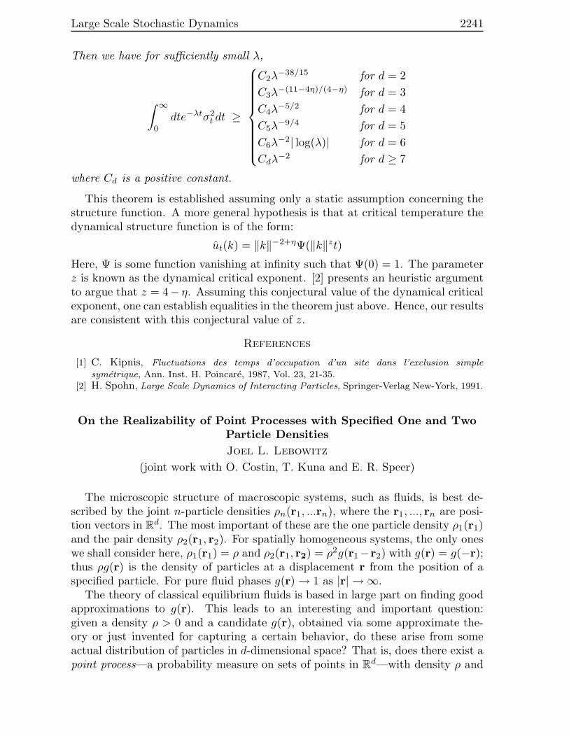
Then we have for sufficiently small λ,

∫ ∞

0

dte−λtσ2t dt ≥

C2λ−38/15 for d = 2

C3λ−(11−4η)/(4−η) for d = 3

C4λ−5/2 for d = 4

C5λ−9/4 for d = 5

C6λ−2| log(λ)| for d = 6

Cdλ−2 for d ≥ 7

where Cd is a positive constant.

This theorem is established assuming only a static assumption concerning thestructure function. A more general hypothesis is that at critical temperature thedynamical structure function is of the form:

ut(k) = ‖k‖−2+ηΨ(‖k‖zt)

Here, Ψ is some function vanishing at infinity such that Ψ(0) = 1. The parameterz is known as the dynamical critical exponent. [2] presents an heuristic argumentto argue that z = 4− η. Assuming this conjectural value of the dynamical criticalexponent, one can establish equalities in the theorem just above. Hence, our resultsare consistent with this conjectural value of z.

References

[1] C. Kipnis, Fluctuations des temps d’occupation d’un site dans l’exclusion simple

symetrique, Ann. Inst. H. Poincare, 1987, Vol. 23, 21-35.[2] H. Spohn, Large Scale Dynamics of Interacting Particles, Springer-Verlag New-York, 1991.

On the Realizability of Point Processes with Specified One and Two

Particle Densities

Joel L. Lebowitz

(joint work with O. Costin, T. Kuna and E. R. Speer)

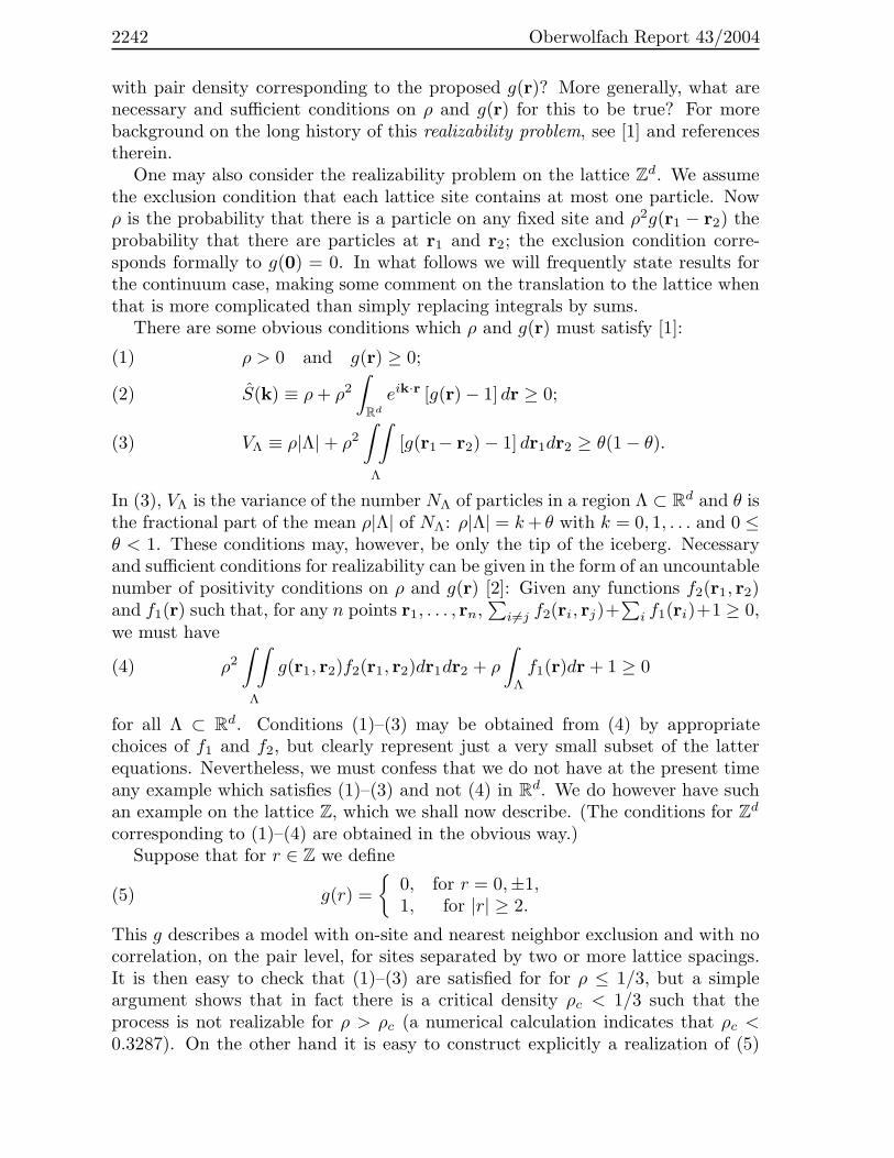
The microscopic structure of macroscopic systems, such as fluids, is best de-scribed by the joint n-particle densities ρn(r1, ...rn), where the r1, ..., rn are posi-tion vectors in Rd. The most important of these are the one particle density ρ1(r1)and the pair density ρ2(r1, r2). For spatially homogeneous systems, the only oneswe shall consider here, ρ1(r1) = ρ and ρ2(r1, r2) = ρ2g(r1−r2) with g(r) = g(−r);thus ρg(r) is the density of particles at a displacement r from the position of aspecified particle. For pure fluid phases g(r) → 1 as |r| → ∞.

The theory of classical equilibrium fluids is based in large part on finding goodapproximations to g(r). This leads to an interesting and important question:given a density ρ > 0 and a candidate g(r), obtained via some approximate the-ory or just invented for capturing a certain behavior, do these arise from someactual distribution of particles in d-dimensional space? That is, does there exist apoint process—a probability measure on sets of points in Rd—with density ρ and


with pair density corresponding to the proposed g(r)? More generally, what arenecessary and sufficient conditions on ρ and g(r) for this to be true? For morebackground on the long history of this realizability problem, see [1] and referencestherein.

One may also consider the realizability problem on the lattice Zd. We assumethe exclusion condition that each lattice site contains at most one particle. Nowρ is the probability that there is a particle on any fixed site and ρ2g(r1 − r2) theprobability that there are particles at r1 and r2; the exclusion condition corre-sponds formally to g(0) = 0. In what follows we will frequently state results forthe continuum case, making some comment on the translation to the lattice whenthat is more complicated than simply replacing integrals by sums.

There are some obvious conditions which ρ and g(r) must satisfy [1]:

ρ > 0 and g(r) ≥ 0;(1)

S(k) ≡ ρ+ ρ2

∫

Rd

eik·r [g(r) − 1]dr ≥ 0;(2)

VΛ ≡ ρ|Λ| + ρ2

∫ ∫

Λ

[g(r1− r2) − 1] dr1dr2 ≥ θ(1 − θ).(3)

In (3), VΛ is the variance of the number NΛ of particles in a region Λ ⊂ Rd and θ isthe fractional part of the mean ρ|Λ| of NΛ: ρ|Λ| = k+ θ with k = 0, 1, . . . and 0 ≤θ < 1. These conditions may, however, be only the tip of the iceberg. Necessaryand sufficient conditions for realizability can be given in the form of an uncountablenumber of positivity conditions on ρ and g(r) [2]: Given any functions f2(r1, r2)and f1(r) such that, for any n points r1, . . . , rn,

∑i6=j f2(ri, rj)+

∑i f1(ri)+1 ≥ 0,

we must have

(4) ρ2

∫ ∫

Λ

g(r1, r2)f2(r1, r2)dr1dr2 + ρ

∫

Λ

f1(r)dr + 1 ≥ 0

for all Λ ⊂ Rd. Conditions (1)–(3) may be obtained from (4) by appropriatechoices of f1 and f2, but clearly represent just a very small subset of the latterequations. Nevertheless, we must confess that we do not have at the present timeany example which satisfies (1)–(3) and not (4) in Rd. We do however have suchan example on the lattice Z, which we shall now describe. (The conditions for Zd

corresponding to (1)–(4) are obtained in the obvious way.)Suppose that for r ∈ Z we define

(5) g(r) =

0, for r = 0,±1,1, for |r| ≥ 2.

This g describes a model with on-site and nearest neighbor exclusion and with nocorrelation, on the pair level, for sites separated by two or more lattice spacings.It is then easy to check that (1)–(3) are satisfied for for ρ ≤ 1/3, but a simpleargument shows that in fact there is a critical density ρc < 1/3 such that theprocess is not realizable for ρ > ρc (a numerical calculation indicates that ρc <0.3287). On the other hand it is easy to construct explicitly a realization of (5)


for ρ ≤ 1/4: Start with a Bernoulli measure on Z with density λ and then removeany particle from an occupied site x if and only if site x+ 1 is also occupied. Thiswill yield a translation invariant state with density ρ = λ(1 − λ) ≤ 1/4 and withg(r) given by (5). Whether (5) is realizable for any ρ > 1/4 (i.e., whether or notρc > 1/4) is a complete mystery to us at present. We can show, however, that thestate constructed above corresponds to a renewal process, for which the sequenceof interparticle distances is Markovian, and that such a renewal process with g(r)given by (5) cannot exist for ρ > 1/4. (The corresponding result on R is discussedin [1], where it is shown that a renewal process exists with

(6) g(r) =

0, for |r| ≤ 1,1, for |r| > 1.

if and only if ρ ≤ 1/e. Here the maximum ρ consistent with (1)–(3) is 1/2.)Let us now state a general theorem about realizability of a given ρ and g(r),

r ∈ Rd.

Theorem: Let

g(r) =

0, |r| ≤ D,exp(−ϕ(r)), |r| > D,

where for some Φ ≥ 0,

(7)

n∑

i=1

ϕ(ri) ≥ −2Φ whenever |ri − rj | ≥ D, 1 ≤ i < j ≤ n.

Then ρ and g(r) are realizable whenever

(8) ρ ≤(e1+2Φ

∫

Rd

|g(r) − 1| dr)−1

.

Note that condition (7) is satisfied for any D ≥ 0 (and Φ = 0) if ϕ(r) ≥ 0 forall r, and for D > 0 (i.e., with a hard core) if ϕ(r) decays faster than |r|−(d+ǫ) for|r| → ∞ [3]. A similar theorem holds in the lattice case Zd; the integral has to bereplaced by a sum and the hard core condition is automatically satisfied becauseat most one particle can occupy any site. The theorem is a generalization of aresult of R. V. Ambartzumian and H. S. Sukiasian (A-S) [4], who considered onlythe case ϕ ≥ 0 (g ≤ 1). For the example (5) the theorem gives existence onlyfor ρ ≤ (3e)−1, so it is clearly not optimal. Readers with a statistical mechanicsbackground will recognize the right hand side of (8) as the Ruelle-Penrose lowerbound for the radius of convergence of the fugacity expansion for an equilibriumsystem with pair potential ϕ given by g(r) = e−ϕ(r) [3].

The construction by A-S of the point process corresponding to ρ and g(r), whichwe follow, does not in general yield a Gibbs measure. The existence of a Gibbsmeasure with a decaying pair potential which realizes a given ρ and g(r) was provenby L. Koralov for lattice gases when ρ is sufficiently small and

∑r|g(r) − 1| < 2

[5]. In general, if any measure realizes ρ and g(r) then we can ask for the measurewhich maximizes the entropy subject to the constraint of the given ρ and g; this


should “formally” be a Gibbs measure with some pair potential [6]. There is noguarantee, however, that this potential would have any good decay property.

Acknowledgments: We thank S. Goldstein and S. Torquato for many usefuldiscussions.

References

[1] O. Costin and J. L. Lebowitz. On the Construction of Particle Distribution with SpecifiedSingle and Pair Densities. Preprint: Los Alamos cond-mat/0405519. To appear in Journalof Physical Chemistry.

[2] T. Kuna, J. L. Lebowitz, and E. Speer, in preparation.[3] D. Ruelle, Statistical Mechanics: Rigorous Results (World Scientific, Imperial College Press,

London, 1999).[4] R. V. Ambartzumian and H. S. Sukiasian. Inclusion-Exclusion and Point Processes. Acta

Appl. Math. 22, (1991).[5] L. Koralov. The existence of Pair Potential Corresponding to Specified Density and Pair

Correlation. Preprint, Princeton University, 2004.[6] S. R. S. Varadhan, private communication.

Stochastic lattice gases with dynamical constraints and glassy

dynamics

Cristina Toninelli

(joint work with G.Biroli and D.S.Fisher)

I report results obtained in collaboration with G.Biroli and D.S.Fisher [9, 11, 10,12] on some kinetically constrained lattice gases introduced in physical literature tostudy glassy dynamics (see for review [6]). These are stochastic lattice gases withhard core constraint and dynamics given by a continuous time Markov processwhich consists of a sequence of particle jumps. The rates are chosen in order toimpose additional constraints (beyond hard core) to the allowed moves, namelythe jump from x to y can have zero rate even if y is empty. This is an attempt tomimic the geometric constraints on the moves of a molecule in a dense liquid dueto neighboring molecules. These constraints could indeed cooperatively producea dramatic slowing down of dynamics at a finite density leading to liquid-glasstransition, a phenomenon which still remains to be understood.

I will focus on a class of models (KA) which were introduced in [4]. Let Λ ⊂ Zd

and m ∈ 1, . . . , 2d − 1, a configuration is defined by giving for each x ∈ Λ theoccupation number ηx ∈ 0, 1. The rate cx,y(η) for the jump from x to y is equalto one if: i) y is nearest neighbor to x ii) and y is empty iii) and no more thanm nearest neighbors of x are occupied iv) and no more than m nearest neighborsof y different from x are occupied. If one or more of the above constraints is notsatisfied the jump is not allowed, namely cx,y(η) = 0. Note that for m = 0 wewould recover the symmetric simple exclusion process (SSEP).

On a finite volume dynamics preserves the number of particles and the ratessatisfy the detailed balance w.r.t. the uniform measure νΛ,N on the hyperplane


ΩΛ,N with N particles. Therefore the generator is reversible w.r.t. νΛ,N andthese are stationary measures. However, due to the degeneracy of rates, they arenot the unique invariant measures. Indeed there exist configurations which donot evolve under dynamics and all measures concentrated on such configurationsare invariant too. For instance, if d = 2 and m = 1, frozen configurations canbe constructed by noticing that all the particles belonging to two fully occupiedconsecutive rows are forever blocked. Therefore the process is not ergodic on ΩΛ,N ,which decomposes into disconnected irreducible components. On the other handon infinite volume, i.e. for Λ = Zd, the rates satisfy detailed balance with respectto Bernoulli product measure µρ at any ρ ∈ [0, 1]. A key question is whether theprocess is ergodic in L2(µρ), i.e. if zero is a simple eigenvalue of the generator. Inthis case spectral theorem would guarantee that time averages of local quantitiesconverge in the long time limit to averages over the equilibrium ensemble µρ. Ifthe process is ergodic for ρ ≤ ρc and not ergodic for ρ > ρc we say that andergodic/non-ergodic transition occurs at ρc. From numerical simulations [4] it hasbeen conjectured that such a transition occurs at ρc ≃ 0.881 for the model onthe cubic lattice with m = 3. Analogous ergodicity breaking transitions have beenfound in different approximate theories for supercooled liquids (e.g. mode couplingtheory and random first order scenario) and have been advocated as the cause ofthe slowing down of dynamics and the onset of liquid-glass transition.

Another relevant issue is the asymptotic displacement of a tagged particle.Indeed, for many supercooled liquids, a striking decrease of the mean square dis-placement of the tracer occurs near the glass transition [2]. For KA model, aslong as the process is ergodic, a central limit theorem holds [3] and the positionof the tagged particle in equilibrium converges, under diffusive space-time rescal-ing, to Brownian motion with a density dependent self-diffusion coefficient DS(ρ).This is expressed by a variational formula as in [7]. However, due to the degen-eracy of rates, one cannot extend the strict positiveness for such formula provenfor SSEP in [7]. Furthermore, from simulations it has been conjectured that adiffusive/sub–diffusive transition takes place at a critical density ρ, with DS = 0for ρ > ρ. Indeed, on the cubic lattice with m = 3, data were found to fit wellwith a transition at ρ ≃ 0.881 and DS ∝ (ρ− ρ)3.1 for ρ→ ρ from below [4].

Our first result [9, 11, 12] is that, for any value of the spatial dimension d andthe parameter m, an ergodic/non-ergodic transition does not occur at a non-trivialdensity ρ ∈ (0, 1). More precisely, for m ≤ d−1 the process on the infinite volumeis not ergodic at any ρ ∈ (0, 1], while form > d−1 ergodicity holds at any ρ ∈ [0, 1).The first statement can be easily established by noticing that, if m ≤ d − 1, anyfully occupied hypercube of particles can never be broken, therefore at any ρ thereexists a finite fraction of frozen particles. In the following we will focus on themodels with m > d, which are the interesting ones for the physical problem. Inthese cases, through the construction of allowed paths among configurations, onecan identify an irreducible component which has unit probability w.r.t. any µρ

with ρ < 1. This, together with the product form of Bernoulli measure, allowsto establish ergodicity. Therefore, on any finite lattice the process is not ergodic


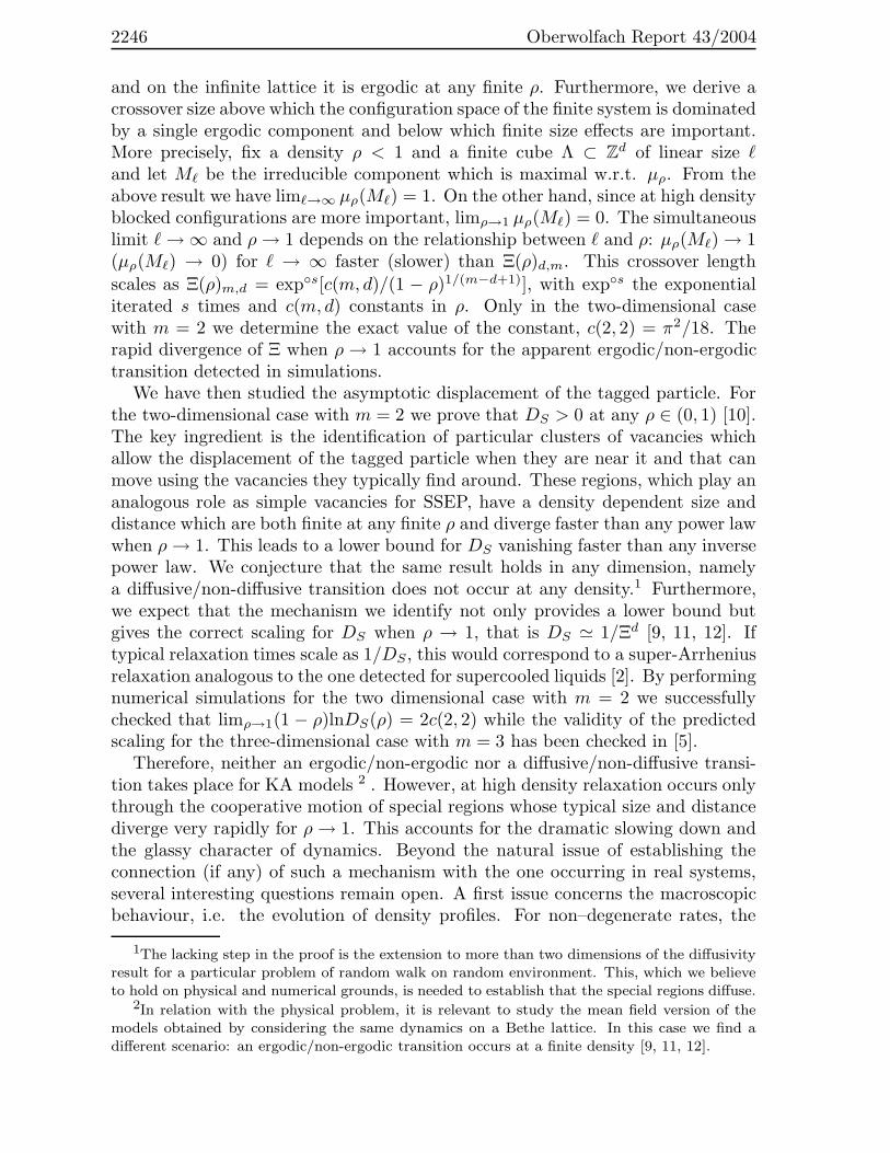
and on the infinite lattice it is ergodic at any finite ρ. Furthermore, we derive acrossover size above which the configuration space of the finite system is dominatedby a single ergodic component and below which finite size effects are important.More precisely, fix a density ρ < 1 and a finite cube Λ ⊂ Zd of linear size ℓand let Mℓ be the irreducible component which is maximal w.r.t. µρ. From theabove result we have limℓ→∞ µρ(Mℓ) = 1. On the other hand, since at high densityblocked configurations are more important, limρ→1 µρ(Mℓ) = 0. The simultaneouslimit ℓ→ ∞ and ρ→ 1 depends on the relationship between ℓ and ρ: µρ(Mℓ) → 1(µρ(Mℓ) → 0) for ℓ → ∞ faster (slower) than Ξ(ρ)d,m. This crossover length

scales as Ξ(ρ)m,d = exps[c(m, d)/(1 − ρ)1/(m−d+1)], with exps the exponentialiterated s times and c(m, d) constants in ρ. Only in the two-dimensional casewith m = 2 we determine the exact value of the constant, c(2, 2) = π2/18. Therapid divergence of Ξ when ρ → 1 accounts for the apparent ergodic/non-ergodictransition detected in simulations.

We have then studied the asymptotic displacement of the tagged particle. Forthe two-dimensional case with m = 2 we prove that DS > 0 at any ρ ∈ (0, 1) [10].The key ingredient is the identification of particular clusters of vacancies whichallow the displacement of the tagged particle when they are near it and that canmove using the vacancies they typically find around. These regions, which play ananalogous role as simple vacancies for SSEP, have a density dependent size anddistance which are both finite at any finite ρ and diverge faster than any power lawwhen ρ→ 1. This leads to a lower bound for DS vanishing faster than any inversepower law. We conjecture that the same result holds in any dimension, namelya diffusive/non-diffusive transition does not occur at any density.1 Furthermore,we expect that the mechanism we identify not only provides a lower bound butgives the correct scaling for DS when ρ → 1, that is DS ≃ 1/Ξd [9, 11, 12]. Iftypical relaxation times scale as 1/DS, this would correspond to a super-Arrheniusrelaxation analogous to the one detected for supercooled liquids [2]. By performingnumerical simulations for the two dimensional case with m = 2 we successfullychecked that limρ→1(1 − ρ)lnDS(ρ) = 2c(2, 2) while the validity of the predictedscaling for the three-dimensional case with m = 3 has been checked in [5].

Therefore, neither an ergodic/non-ergodic nor a diffusive/non-diffusive transi-tion takes place for KA models 2 . However, at high density relaxation occurs onlythrough the cooperative motion of special regions whose typical size and distancediverge very rapidly for ρ → 1. This accounts for the dramatic slowing down andthe glassy character of dynamics. Beyond the natural issue of establishing theconnection (if any) of such a mechanism with the one occurring in real systems,several interesting questions remain open. A first issue concerns the macroscopicbehaviour, i.e. the evolution of density profiles. For non–degenerate rates, the

1The lacking step in the proof is the extension to more than two dimensions of the diffusivityresult for a particular problem of random walk on random environment. This, which we believeto hold on physical and numerical grounds, is needed to establish that the special regions diffuse.

2In relation with the physical problem, it is relevant to study the mean field version of themodels obtained by considering the same dynamics on a Bethe lattice. In this case we find adifferent scenario: an ergodic/non-ergodic transition occurs at a finite density [9, 11, 12].


hydrodynamical limit [8] states that the coarse-grained density profile evolves un-der a diffusion equation ∂tρ = ∇ (D(ρ)∇ρ). Although we conjecture that on largeenough length and time scales hydrodynamics will be valid at any ρ < 1 for ergodicKA models, this seems to be hard to prove due to the degeneracy of rates. If theconjecture is correct, another issue related to both experiments and simulations[1] of glass-forming liquids, is the characteristic length and time scales beyondwhich hydrodynamic behavior sets in and how these increase with density. Otheropen questions are related to relaxation towards equilibrium. A natural quantityto consider is the dynamical structure factor F (k, t), i.e. the Fourier transform ofthe density-density correlation function at non-zero wave vector. For the simplesymmetric exclusion, F (k, t) decays exponentially at long times [8]. For KA mod-els numerical simulations suggest that relaxation could be slower than exponential(at least above some critical density). The decay is usually fitted by a stretchedexponential F (k, t) ∼ exp[−(t/τ(k))β ], with β < 1 [5]. This is again reminiscentto the anomalous decay occurring at sufficiently low temperature in many glass-forming liquids [2] and understanding whether and why this occurs for kineticallyconstrained models could be very useful.

References

[1] Berthier Time and length scales in supercooled liquids Phys. Rev. E 69 (2004) 020201(R).[2] De Benedetti P.G. Metastable liquids. Princeton University Press 1997.[3] Kipnis C., Varadhan S.R.S. Central limit theorem for additive functionals of reversible

Markov processes and applications to simple exclusions. Comm. Math. Phys. 104 (1986)1.[4] Kob W, Andersen H, Phys. Rev. E, Kinetic lattice-gas model of cage effects in high density

liquids and a test of mode-coupling theory of the ideal glass transition 48, (1993) 4364[5] Marinari E, Pitard E, A Topographic-Non-Topographic Paradigm for Glassy Dynamics,

preprint cond-mat/0404214.[6] Ritort F, Sollich P Glassy dynamics of kinetically constrained models Adv.in Phys. 52,

(2003) 219[7] Spohn H. Tracer diffusion in lattice gases. J. Statist. Phys. 59 (1990), 1227–1239.[8] Spohn H. Large scale dynamics of interacting particles. Berlin: Springer 1991.[9] Toninelli C, Biroli G, Fisher D.S. Spatial structures and dynamics of kinetically constrained

models for glasses Phys.Rev.Lett. 92. 185504 (2004).[10] Toninelli C, Biroli G Dynamical arrest, tracer diffusion and kinetically constrained lattice

gases preprint cond-mat/0402314 to appear on J.Stat.Phys.[11] Toninelli C, Biroli G and Fisher D.S. Cooperative behaviour of kinetically constrained lattice

gas models of glassy dynamics preprint.[12] Toninelli C Kinetically constrained models and glassy dynamics PHD thesis Univ. la

Sapienza di Roma, October 2003.


Local Functional of Phase Separation Lines

Dmitry Ioffe

1. Introduction

For a large class of two-dimensional low temperature models of statistical me-chanics in the phase co-existence regime the probabilistic structure of phase sep-aration lines falls in the general framework of the thermodynamic formalism ofsub-shifts over countable alphabets. In this way statistical weights of phase bound-aries are reinterpreted in terms of actions of Ruelle type operators with Lipschitzcontinuous potentials and a local limit characterization of various observables ofthese phase boundaries follows from from a spectral analysis of the latter. Recentadvances include a comprehensive implementation of such approach in the case ofthe nearest neighbour Ising model model at all sub-critical temperatures.

Below I shall give examples of results which could be obtained along these linesand try to stipulate a rather general features of the statistical weights on whichthe theory relies.

2. Ising model in a strip

A canonical example of phase separation lines is given in the framework of thenearest neighbour two dimensional Ising model below the critical temperature Tc.Let

S∗N = (1/2, 1/2) + [0, . . . , N − 1] × Z ⊂ Z2∗

be an infinite dual strip of width N . A spin configuration σ on S∗N is an element

of −1, 1S∗N . Consider the so called Dobrushin’s boundary conditions

σ(y1, y2) = 1Iy2>0 − 1Iy2<0.

Every σ ∈ −1, 1S∗N gives rise to the set of microscopic boundaries between re-

gions occupied by spins of different signs. Using a “rounding of corners” procedure[DKS] contours can be represented as either open or closed self-avoiding curvesin R2. In fact to each σ there corresponds precisely one open crossing contourγ = γ[σ] with end points at 0 and (N, 0)

The contour γ models the ~e1-oriented microscopic interface between co-existingphases of the nearest neighbour Ising model at the inverse temperature β > βc,where βc = 1/Tc is the phase transition threshold. The statistics P±

N,β of γ is

read from the Ising Gibbs distribution on −1,+1S∗N under Dobrushin boundary

conditions σ defined above.

3. Large scale structure of γ

Our first result is an invariance principle for the interface γ under the diffusivescaling. Similar results were previously obtained at very low temperatures usingthe method of cluster expansions [DH, Ga, Hi]. Let γN be the scaling of γ by


1/N in the horizontal (role of time) direction and by 1/√N in the vertical (role

of space) direction.

Theorem 3.1. For every β > βc the distribution of γN under P±N,β weakly con-

verges on C0[0, 1] to the distribution of√κβB(·), where B(·) is the standard Brown-

ian bridge and κβ is the curvature of the boundary β- equilibrium crystal shape inthe horizontal direction.

The theorem has been proved in [GI], actually for Ising interfaces stretched inarbitrary directions.

4. CLT for local functionals of γ

We continue to work with the Ising model on a strip with Dobrushin boundaryconditions. Each crossing contour γ = γ[σ] splits S∗

N into the upper (positive b.c.)part and the lower (negative b.c) part. Let χx(σ) = ±1 be the indicator that xblies in the ± part. A general approach to local anti-symmetric functionals of γ hasbeen developed in [HIK]. Here I give two examples:

4.1. Excess magnetization. For x ∈ S∗N let < σ(x)|γ >N,β be the conditional

expectation given that γ is the crossing contour of σ. Let also m∗N (x) be the

expectation of σ(x) under the pure + boundary conditions on ∂S∗N . Consider the

quantity,

∆N (σ) =∑

x∈S∗N

(< σ(x)|γ >N,β −χx(σ)m∗N (x)) .

Theorem 4.1. The random variable ∆N/√N is asymptotically normal.

4.2. Glauber dynamics. Let L be a generator of Glauber dynamics on −1, 1S∗N

reversible with respect to P±N,β. Define the signed area under the (random) inter-

face γ as AN (γ) = AN(σ).

Theorem 4.2. The random variable LAN (σ)/√N is asymptotically normal.

5. Properties of statistical weights

The probability distribution P±N,β is based on statistical weights qβ (γ) on phase

separation lines γ. A simplifying feature of the two dimensional Ising model is thatthese weights can be related by duality to the statistical weights which appearin the high temperature expansion [CIV1, CIV2, PV]. On the other hand, theOrnstein-Zernike theory developed in [CIV1] relies on the following four propertiesof qβ (·):Strict exponential decay of the two-point function: There exists C1 < ∞such that, for all x ∈ Zd \ 0,

∑

λ: 0→x

qβ(λ) < C1 e−|x|/C1.


Finite energy condition: For any pair of compatible paths λ and η define theconditional weight

q(λ | η) = q(λ ∐ η)/q(η)

where λ ∐ η denotes the concatenation of λ and η. Then there exists a universalfinite constant C2 < ∞ such that the conditional weights are controlled in termsof path sizes |λ| as:

q(λ | η) < e−C2|λ| .

BK-type splitting property: There exists C3 < ∞, such that, for all x, y ∈Zd \ 0 with x 6= y,

∑

λ: 0→x→y

q(λ) < C3

∑

λ: 0→x

q(λ)∑

λ: x→y

q(λ) .

Exponential mixing : There exists C4 < ∞ and θ ∈ (0, 1) such that, for anyfour paths λ, η, γ1 and γ2, with λ∐ η ∐ γ1 and λ∐ η ∐ γ2 both admissible,

q(λ | η ∐ γ1)

q(λ | η ∐ γ2)< expC4

∑

x∈λy∈γ1∪γ2

θ|x−y| .

References

[CIV1] M. Campanino, D. Ioffe, Y. Velenik (2003), Ornstein-Zernike theory for finite range Isingmodels above Tc, Probab. Theory Related Fields 125, 3, 305–349.

[CIV2] M. Campanino, D. Ioffe, Y. Velenik (2003), Random path representation and sharp cor-relation asymptotics at high temperatures, to appear in Advanced Studies in Pure Math-ematics.

[DH] R. Dobrushin, O. Hryniv (1997), Fluctuations of the phase boundary in the 2D Isingferromagnet , Comm. Math. Phys. 189, 2, 395–445.

[DKS] R. Dobrushin, R. Kotecky, S. Shlosman (1992), Wulff construction. A global shape fromlocal interaction., Translations of Mathematical Monographs 104, American Mathemat-ical Society, Providence.

[Ga] G. Gallavotti (1972), The phase separation line in the two-dimensional Ising model ,Commun. Math. Phys. 27, 103–136.

[GI] L. Greenberg, D. Ioffe (2004), On an invariance principle for phase separation lines, toappear in AIHP, Probability and Statistics.

[Hi] Y. Higuchi (1979), On some limit theorem related to the phase separation line in thetwo-dimensional Ising model , Z.Wahrsch.Verw.Gebiete, 50, 3, 287–315.

[HIK] O. Hryniv, D. Ioffe, R. Kotecky (2004), Local anti-symmetric functionals of phase sepa-ration lines, in preparation.

[Hr] O. Hryniv (1998), On local behaviour of the phase separation line in the 2D Ising model ,Probab. Theory Related Fields 110, 1, 91–107.

[PV] C.-E. Pfister, and Y. Velenik (1999), Interface, surface tension and reentrant pinningtransition in the 2D Ising model, Comm. Math. Phys. 204, no. 2, 269–312.


Current fluctuations in non-equilibrium diffusive systems

Thierry Bodineau

(joint work with Bernard Derrida)

Understanding the fluctuations of the steady state current through a systemin contact with two (or more) heat or particle reservoirs is one of the naturalquestions arising in non-equilibrium physics [6, 5, 11]. We report on the paper [4]where a functional for the current large deviations was proposed.

We consider a one dimensional diffusive open system of length N (with N large)in contact, at its two ends, with two reservoirs of particles at densities ρa and ρb.In the bulk, the system evolves under some conservative stochastic dynamics and,at the boundaries, particles are created or annihilated to match the densities ofthe reservoirs. Let Qt be the integrated current up to time t, i.e. the numberof particles which went through the system during time t. The large deviationfunctional G associated to Qt can be written as

limt→∞

limN→∞

1

tNlog

⟨QtN2

tN∼ q

⟩= −G(q, ρa, ρb) ,

where we used a diffusive scaling.

First of all, we would like to provide a heuristic derivation of the functionalG by thermodynamical considerations. This is based on the assumption that Gsatisfies the following additivity principle. If we split a system of macroscopic unitlength into two parts of lengths x and 1 − x, then we assume that

G(q, ρa, ρb) = maxρ

G(qx, ρa, ρ)

x+G(q(1 − x), ρ, ρb)

1 − x

.(1)

The idea of factorizing a partition function as the product of partition functionsin sub-domains may look innocuous from the perspective of equilibrium statisticalmechanics, however such property is not true in general. In particular the densitylarge deviation functional associated to the steady is not additive (see [7]). Theassumption behind (1) is that conditioned on the current deviation q, the systemremains essentially close to a fixed profile over a long period of time. This profileis chosen in order to facilitate the current deviations and is a solution of thevariational principle (5).

The next step is to introduce the two macroscopic parameters from which thefunctional can be recovered. Suppose that for ρa = ρ + ∆ρ and ρb = ρ with ∆ρsmall, the diffusion coefficient D(ρ) satisfies Fick’s law

〈Qt〉t

=1

ND(ρ) ∆ρ .(2)

Suppose that for ρa = ρb = ρ the variance of the current can expressed in termsof the conductivity σ(ρ)

〈Q2t 〉t

∼ 1

Nσ(ρ) .(3)


If we keep dividing the system into smaller and smaller pieces and assume thatfor a piece of small (macroscopic) size ∆x (i.e. of N∆x sites), the behavior isessentially gaussian

1

∆xG(q∆x, ρ, ρ+ ∆ρ) ≃ − [q∆x+D(ρ)∆ρ]

2

2σ(ρ)∆x,(4)

thus one finds a variational form for G

G(q, ρa, ρb) = minρ(x)

[∫ 1

0

[q +D(ρ(x))ρ′(x)

]2

2σ(ρ(x))dx

],(5)

where the minimum is over all the functions ρ(x) with boundary conditions ρ(0) =ρa and ρ(1) = ρb.

For systems of purely classical interacting particles [11] in contact with tworeservoirs the theory is, to our knowledge, less developed. However, one maywonder whether similar additivity principle pertains in this context and whethersome universal features can be predicted by the formula (5). Notice also that theadditivity principle can be used to study more complex diffusive networks includingloops and that the expression (5) satisfies the Gallavotti-Cohen symmetry [8].

A mathematical justification of (5) can be achieved for some stochastic dynam-ics by using the formalism of hydrodynamic large deviations (see [10, 12]). Inparticular for the SSEP, the variational principle (5) can be recovered and theadditivity principle justified a posteriori. In general only the space/time versionof (5) is valid, i.e. that the exponential cost of observing a current profile q(x, t)over a period [0, T ] and a density profile ρ(x, t) such that ∂tρ = −∇xq is given by

G(q, ρ) =

∫ T

0

dt

∫ 1

0

dx

[q(x, t) +D(ρ(x, t))ρ′(x, t)

]2

2σ(ρ(x, t)).(6)

Observing a mean current q = 1T

∫ T

0dt∫ 1

0dx q(x, t) amounts to integrate (6) over

time and this cannot always be reduced to (5). This was understood by Bertini,De Sole, Gabrielli, Jona–Lasinio, Landim [3] who introduced a multi-dimensionalextension of (6) and exhibit a counter-example of (5) for a specific choice of Dand σ.

References

[1] L. Bertini, A. De Sole, D. Gabrielli, G. Jona–Lasinio, C. Landim, Macroscopic fluctuationtheory for stationary non equilibrium states, J. Stat, Phys. 107, 635-675 (2002)

[2] L. Bertini, A. De Sole, D. Gabrielli, G. Jona–Lasinio, C. Landim, Large deviations for the

boundary driven symmetric simple exclusion process, Math. Phys. Analysis and Geometry6, 231-267 (2003)

[3] L. Bertini, A. De Sole, D. Gabrielli, G. Jona–Lasinio, C. Landim, Macroscopic currentfluctuations in stochastic lattice gases, cond-mat/0407161.

[4] T. Bodineau, B. Derrida, Current fluctuations in non-equilibrium diffusive systems: anadditivity principle, Phys. Rev. Lett. 92, 180601 (2004).

[5] F. Bonetto, J.L. Lebowitz, L. Rey-Bellet, Fourier’s law: a challenge to theorists, Mathemat-ical Physics 2000, 128-150, 2000, Imperial College Press, math-ph/0002052


[6] B. Derrida, B. Doucot, P.-E. Roche, Current fluctuations in the one dimensional symmetricexclusion process with open boundaries J. Stat. Phys. 115, 717 (2004)

[7] B. Derrida, J.L. Lebowitz, E.R. Speer, Large Deviation of the Density Profile in the SteadyState of the Open Symmetric Simple Exclusion Process J. Stat. Phys. 107, 599 (2002).

[8] G. Gallavotti, E.D.G. Cohen, Dynamical ensembles in stationary states, J. Stat. Phys. 80,931-970 (1995)

[9] A. Jordan, E. Sukhorukov, S. Pilgram, Fluctuation Statistics in Networks: a StochasticPath Integral Approach, preprint cond-mat/0401650

[10] C. Kipnis, C. Landim, Scaling limits of interacting particle systems (Springer-Verlag, Berlin,1999).

[11] S. Lepri, R. Livi, A. Politi, Thermal conduction in classical low-dimensional lattices, Phys.Rep. 377, 1-80 (2003)

[12] H. Spohn, Large Scale Dynamics of Interacting Particles (Springer-Verlag, Berlin, 1991)

The directed polymer in random environment is diffusive at weak

disorder

Francis Comets

(joint work with Nobuo Yoshida)

In this popular model, the polymer is a long chain of size n which is stretchesin one particular direction of Zd+1, and is modelled as a nearest neighbor pathin Zd. The environment is given by independent identically distributed randomvariables η(n, x), with all finite exponential moments. The polymer is attractedby large positive values of the environment, and repelled by large negative ones.All these considerations lead to the polymer measure:

µn(dω) = Z−1n expβ

n∑

t=1

η(t, ωt) P (dω)

with P the distribution of the simple random walk on the integer lattice Zd,β ∈ [0,∞) a “temperature inverse” prescribing how strongly the polymer path ωinteracts with the medium, and Zn the normalizing constant making µn a prob-ability measure on the path space. Note the measure µn depends on n, β and onthe environment η.

The issue is to study the asymptotics of the polymer ω as n → ∞ underthe measure µn, for typical realization of the environment; In particular, one isinterested in the exponent ξ ∈ [1/2, 1) such that

|ωn| is of order nξ

as n → ∞. The ground states (limit as β → ∞) of the model is the oriented lastpassage percolation model, for which it is known, for d = 1 and very few specificcases for the distribution of η, that ξ = 2/3 ([7], [10]): the path is superdiffusive,in contrast with the simple random walk which is diffusive (corresponding to ξ =1/2). Another quantity of interest is the exponent χ ∈ [0, 1/2] for the fluctuationsof the normalizing constant, i.e. such that

lnZn − an is of order nχ for some constant an


as n → ∞. A number of predictions, conjectures and numerical estimates canbe found in the physical literature [5], [8], on the values on such exponents, andrelations between them. In particular, the scaling relation

χ = 2ξ − 1

is believed to hold. In fact, for d = 1, β = ∞ and a few specific cases for thedistribution of η, χ, it is proven that χ = 1/3, i.e., the scaling relation holds inthis case.

Weak and Strong disorder: Bolthausen [1] considered the positive martin-gale Zn/EZn converges almost surely, and that a dychotomy takes place:

limnZn/EZn

> 0 a.s.or

= 0 a.s.

A natural manner for measuring the disorder due to the random environment,is to call weak disorder the first case, and strong disorder the second one.Note that weak disorder can be defined as the region where χ = 0 and an =n lnE[expβη(t, x)]. The terminology is justified, since the former case happens inlarge enough dimension for small β (including β = 0), and the latter case for largeβ and general unbounded environment. A more precise statement is given in thenext theorem. But first, the reader should be warned that weak disorder is notequivalent to small β: Indeed, in dimension d = 1 or 2, strong disorder holds forall β non-zero ([2], [3]).

Theorem: ([6] and [1]) Assume d ≥ 3 and β small enough so that

E(exp 2βη(t, x))

(E expβη(t, x))2× P (∃n > 0 : ωn = 0) < 1 .

Then, weak disorder holds and, for almost every realization of the environment,

the rescaled path ω(n), t → ω(n)t := n−1/2ωnt, converges in law under µn to the

Brownian motion with diffusion matrix d−1Id.

This result was quite a surprise for the scientific community who did not expectthat diffusivity could take place!

The second moment method was used to derive the theorem. The assumptionon β means that the above martingale is bounded in L2, and it is far from beingnecessary. To improve on it, it was necessary to wait for fifteen year: In thefollowing criterium, the crucial quantity is

In = µ⊗2n−1(ωn = ωn) ,

i.e., the probability for two polymers ω and ω independently sampled from thepolymer measure, to meet at time n.

Theorem: ([2] for the gaussian case, [3] for the general case). For non-zero βit holds


limnZn/EZn = 0

=∑

n

In = ∞

almost surely.

The result is obtained by writing the semi-martingale decomposition oflnZn/EZn, and studying separately the terms. This is a refined (conditional) sec-ond moment condition, and the criterium can also be used to obtain quantitativeinformation on the polymer measure itself, on its concentration and localization.

Now, it is natural to conjecture that diffusive behavior takes place in the fullweak disorder region. This indeed what we prove in this work in progress.

Theorem: Assume d ≥ 3 and weak disorder. For all bounded continuousfunction F on the path space, we have

limnµn[F (ω(n))] = EF (B)

in probability. (B is the Brownian motion with diffusion matrix d−1Id.)

The statement shows that indeed the scaling relation holds in the full weakdisorder region.

In the proof we introduce an infinite time horizon measure on the path spacewhich is a natural limit of the sequence µn. This measure is a time inhomoge-neous Markov chain which depends on the environment. We cannot prove thecentral limit theorem for this Markov chain directly. We need to average overthe environment. In order to prove convergence in probability with respect tothe environment, we use again a second moment method by introducing a secondindependent copy of the polymer before performing this average. All through, wemake use of the convergence of the series

∑In as the main technical ingredient.

To finish with, we mention an interesting open (so far) question. Does strongdisorder imply super-diffusivity? For instance, what happens in the case of smalldimension d and small β is not clear at all.

References

[1] Bolthausen, E.: A note on diffusion of directed polymers in a random environment, Com-mun. Math. Phys. 123 (1989) 529–534.

[2] Carmona, P., Hu Y.: On the partition function of a directed polymer in a random environ-ment. Probab. Theory Related Fields 124 (2002) 431–457.

[3] Comets, F., Shiga, T., Yoshida, N. Directed Polymers in Random Environment: Path Lo-calization and Strong Disorder. Bernoulli 9 (2003) 705–723.

[4] Derrida, B. and Spohn, H. : Polymers on disordered trees, spin glasses, and traveling waves.J. Statist. Phys., 51 (1988), 817–840.

[5] Fisher, D. S., Huse, D. A. : Directed paths in random potential, Phys. Rev. B, 43 (1991),10 728 –10 742.

[6] Imbrie, J.Z., Spencer, T.: Diffusion of directed polymer in a random environment, J. Stat.Phys. 52, (1998) 609-626.

[7] Johansson, K.: Shape fluctuations and random matrices. Comm. Math. Phys. 209 (2000)437–476.


[8] Krug, H. and Spohn, H.: Kinetic roughening of growing surfaces. In: Solids Far fromEquilibrium, C. Godreche ed., Cambrige University Press, 1991.

[9] Piza, M.S.T.: Directed polymers in a random environment: some results on fluctuations, J.Statist. Phys. 89 (1997) 581–603.

[10] Prahofer M., Spohn H.: “Statistical self-similarity of one-dimensional growth processes.”Statistical mechanics: from rigorous results to applications. Phys. A 279 (2000), 342–352.

[11] Song, R., Zhou, X.Y.: A remark on diffusion on directed polymers in random environment,J. Statist. Phys. 85, (1996) 277–289.

Brownian Directed Polymers in Random Environment

Nobuo Yoshida

(joint work with Francis Comets)

We study the thermodynamics of a continuous model of directed polymers inrandom environment. The directed polymer in this model is a d-dimensionalBrownian motion (up to finite time t) viewed under a Gibbs measure which isbuilt up with a Poisson random measure on R+ × Rd (=time × space). Here,the Poisson random measure plays the role of the random environment which isindependent both in time and in space. We now give the definition of the randomGibbs measure which we call the polymer measure.

• The Brownian motion: Let (ωtt≥0, P ) denote a d-dimensional standardBrownian motion. To be more specific, we let the measurable space (Ω,F) beC(R+ → Rd) with the cylindrical σ-field, and P be the Wiener measure on (Ω,F)such that Pω0 = 0 = 1.

• The space-time Poisson random measure: We let η denote the Poisson ran-dom measure on R+ × Rd with the unit intensity, defined on a probability space(M,G, Q).

• The polymer measure: We let Vt denote a “tube”around the graph(s, ωs)0<s≤t of the Brownian path,

(1) Vt = Vt(ω) = (s, x) ; s ∈ (0, t], x ∈ U(ωs),where U(x) ⊂ Rd is the closed ball with the unit volume, centered at x ∈ Rd. Forany t > 0, define a probability measure µt on the path space (Ω,F) by

(2) µt(dω) =exp (βη(Vt))

ZtP (dω),

where β ∈ R is a parameter and

(3) Zt = P [exp (βη(Vt))] .

The model considered here, enables us to use stochastic calculus, with respectto both Brownian motion and Poisson process, leading to handy formulas forfluctuations analysis and qualitative properties of the phase diagram.We discuss:

• The normalized partition function, its positivity in the limit which distin-guishes the weak and strong disorder phases.


• The existence of quenched Lyapunov exponent, its positivity, and its agree-ment with the annealed Lyapunov exponent.

• An almost sure central limit theorem for the Brownian polymer for d ≥ 3 andβ smaller than some β0.

• The longitudinal fluctuation of the free energy and some of its relations withthe overlap between replicas and with the transversal fluctuation of the path.The results here includes an almost sure large deviation principle for the polymermeasure. Our fluctuation results are interpreted as bounds on various exponentsand provide a circumstantial evidence of super-diffusivity in dimension one.

• Relations to the Kardar-Parisi-Zhang equation.

References

[CY1] Comets, F., Yoshida, N. Brownian Directed Polymers in Random Environment To appearin Commun. Math. Phys.

[CY2] Comets, F., Yoshida, N. Some New Results on Brownian Directed Polymers in RandomEnvironment, RIMS Kokyuroku 1386, 50–66, (2004).

[CSY] Comets, F., Shiga, T., Yoshida, N. Probabilistic analysis of directed polymers in randomenvironment: a review, Advanced Studies in Pure Mathematics, 39, 115–142, (2004).

Diffusive behavior of isotropic diffusions in random environment

Ofer Zeitouni

(joint work with Alain-Sol Sznitman)

We present results concerning the asymptotic behavior of isotropic diffusionsin random environment that are small perturbations of Brownian motion. Whenthe space dimension is three or more we prove an invariance principle as well astransience. Our methods also apply to questions of homogenization in randommedia. The proof is based on an induction scheme that propagates from scale toscale a Holder norm control on (truncated) transition probabilities, as well as alarge deviations control on the strength of “traps”.

Precise statements and a description of the main induction step are providedC.R. Acad. Sci. Paris, Ser I, v. 339 (2004), pp. 429–434.

Spontaneous symmetry breaking in a driven two-species lattice gas

Gunter M. Schutz

(joint work with R.D. Willmann and S. Großkinsky)

While single-species driven diffusive systems in one dimension are largely un-derstood, two-species models show a variety of phenomena that are a matter ofcurrent research, such as phase separation and spontaneous symmetry breaking(see [1] for a recent review). The first such model that was shown to exhibitspontaneous symmetry breaking was a model with open boundaries that becameknown as the ’bridge model’ [2, 3]. In this model, two species of particles move


in opposite directions. Although the dynamical rules are symmetric with respectto the two species, two phases with non-symmetrical steady states were found byMonte Carlo simulations and mean-field calculations. While the existence of oneof the phases remains disputed [4, 5], a proof for the existence of the other onewas given for the case of a vanishing boundary rate [6].

All symmetry breaking models considered so far evolve by random sequentialupdate, corresponding to continuous time. We study a discrete time variation ofthe bridge model with parallel sublattice update. The dynamics in the bulk isdeterministic, while stochastic events occur at the boundaries. Thus the complex-ity of the problem is reduced, which allows to elucidate the mechanism by whichspontaneous symmetry breaking occurs in this model as well as to give a proof forthe existence of a symmetry broken phase.

The model considered here is defined on a one-dimensional lattice of length L,where L is an even number. Sites are either empty (0) or occupied by a singleparticle of either species A or B. The dynamics is defined as a parallel sublatticeupdate scheme in two half steps. In the first half-step particles are created andannihilated at the two boundary sites with probability α and β, respectively,

| 0 . . . α−→ |A . . . |B . . . β−→ | 0 . . . (left)

. . . 0 | α−→ . . . B | . . . A | β−→ . . . 0 | (right) .

Note that at each boundary site, either annihilation or creation can take place in agiven time step, but not both. In the bulk, the following hopping processes occurdeterministically between sites 2i and 2i+ 1 with 0 < i < L/2:

A01−→ 0A 0B

1−→ B0 AB1−→ BA.

In the second half-step, these deterministic bulk hopping processes take placebetween sites 2i−1 and 2i with 0 < i ≤ L/2. Note that the dynamics is symmetricwith respect to the two particles species.

Phase diagram

The phase diagram of the model can be explored by Monte Carlo simulations.Two phases are found:

• If α < β, the system exhibits a symmetric steady state. Here, the asymp-totic bulk densities are ρA(i) = 0, ρB(i) = αβ/(α + β) if i is odd, andρA(i) = αβ/(α+ β), ρB = 0 if i is even.

• If α > β, the system resides in the symmetry broken phase. Assume theA particles to be in the majority. Then, the bulk densities in the steadystate are ρB(i) = 0 for all i, ρA(i) = 1 for i even and ρA(i) = 1 − β for iodd, so that the minority species is completely expelled from the system.

Thus, the dynamics of the majority species is as in the single species ASEP withparallel sublattice update. For this system, an analytical expression for the steadystate density in a finite system is known [7]. The density profile of the majorityspecies in the broken phase of the sublattice bridge model equals that of the high


density phase in the sublattice ASEP at the given parameters α and β. Particlesof the expelled species only enter the system by fluctuations exponentially small inthe system size L [8], so a typical symmetry broken configuration is stable againstfluctuations.

To establish spontaneous symmetry breaking we additionally have to show thatsuch a configuration can be reached from a symmetric initial condition within atime which is increasing only algebraically in the system size. Due to the deter-ministic bulk dynamics the state space of the process is not fully connected. Butit is obvious that the empty lattice can be reached from any initial configurationas long as β > 0, so we take this as a symmetric initial condition. When one of theboundary probabilities is 0 or 1, the steady state can be given exactly, consistentwith the above picture. But to avoid degeneracies in the following, we assume α,β ∈ (0, 1) and α > β.

Symmetry breaking dynamics

Starting from the empty lattice, A (B) particles are created at every time stepwith probability α at site 1 (L). Once injected, particles move deterministicallywith velocity 2 (−2). Therefore, at time t = L/2 the system is in a state wherethe density of A (B) particles is α (0) at all even sites and 0 (α) at all odd sites.In this situation both creation and annihilation of particles are possible. However,it turns out that the effect of creation of particles is negligible [8]: Whenever thebulk density of A-particles is above β/2, the deterministic hopping transports onaverage more A-particles towards site L than can be annihilated there. This leadsto the formation of an A-particle jam at the right boundary, blocking the injectionof B-particles, and vice versa a B-particle jam at the left boundary. In these jams,the only source of vacancies is annihilation at the boundaries with probability β.Therefore, in a jam, the density of A (B) particles at even (odd) sites is 1, whilethat at odd (even) sites is 1−β. In each time step, the number of particles in eachof the two jams reduces by one with probability β. Due to fluctuations, one of thejams, say the B-jam at the left boundary, is dissolved first. Then A-particles startto reenter at the left boundary. Let ∆N1 be the number of entered A-particlesuntil the A-jam on the right boundary is dissolved. At this point the system isagain empty except for the ∆N1 entered A-particles and some finite fluctuations,and the process of filling the lattice restarts. This establishes a cyclic behaviorand we summarize the main steps of the next cycle.

1. There are ∆N1 A-particles in the system.2. The A-particles reach the right boundary and block the entrance of B’s.

A-particles still enter with probability α and exit with probability β < α, furtherincreasing the majority of A particles.

3. The B-particles reach the left boundary, blocking also the entrance of A’s.4. The jam of B-particles is dissolved and A particles start to reenter.

Again, since α > β the majority of A-particles is increased and when the A-jamat the right boundary is dissolved, the cycle is finished and starts with initial


condition ∆N2 > ∆N1. The initial process from the empty lattice is a cyclewith ∆N0 = 0, and of course ∆N1 ∈ [−L/2, L/2] can also be negative due to

symmetry. But conditioning on a typical outcome ∆N1 = O(√L) of the first cycle

this fluctuation will be amplified after steps 2 and 4. This picture can be maderigorous and one can show that

⟨∆Nk+1 − ∆Nk

∣∣∆Nk

⟩= 2(α/β − 1

)∆Nk +O(1) .

Thus, for α < β the expected value of ∆Nk+1 −∆Nk is proportional to −∆Nk forα < β. Fluctuations are strongly damped, leading to a symmetric phase. On theother hand for α > β the difference is proportional to +∆Nk and thus fluctuationsare amplified towards one of the boundaries of the domain [−L/2, L/2]. Once theboundary is reached, the amplification loop stops and one of the species will re-main expelled from the system. The number of cycles to reach this symmetrybroken phase from a symmetric initial condition is of order logL and the time fora cycle of order L, which yields an algebraic dependence.

We presented the sketch of a proof of spontaneous symmetry breaking for aversion of the bridge model with deterministic bulk dynamics. The amplificationloop sheds new light on the mechanism of symmetry breaking also for modelswith stochastic bulk dynamics, where rigorous statements are only available fordegenerate boundary rates.

References

[1] G. M. Schutz. J. Phys. A, 36:R339, 2003.[2] M. R. Evans, D. P. Foster, C. Godreche, and D. Mukamel. Phys. Rev. Lett, 74:208, 1995.[3] M. R. Evans, D. P. Foster, C. Godreche, and D. Mukamel. J. Stat. Phys., 80:69, 1995.[4] M. Clincy, M. R. Evans, and D. Mukamel. J. Phys. A, 44:9923, 2001.[5] P. F. Arndt, T. Heinzel, and V. Rittenberg. J. Phys. A, 31:L45, 1998.[6] C. Godreche, J. M. Luck, M. R. Evans, D. Mukamel, S. Sandow, and E. R. Speer. J. Phys.

A, 28:6, 1995.[7] G. Schutz. Phys. Rev. E, 47:4265, 1993.[8] R. D. Willmann, G. M. Schutz, and S. Großkinsky. 2004.

Hyperbolic scaling problems: The method of compensated

compactness

Jozsef Fritz

(joint work with Balint Toth)

Historical remarks: A simple system with hyperbolic scaling is given by rk =(1/2)(V ′(rk+1)−V ′(rk−1)) , where V ∈ C2(R) is convex at infinity, rk ∈ R andk ∈Z . At a first glance ρǫ(t, x) := rk(t/ǫ) if |x − kǫ| < ǫ/2 solves ∂tρ = ∂xV

′(ρ)as ǫ → 0. However, the first computer experiments performed by von Neumannand coworkers [11] demonstrated that this numerical procedure does not convergeat all; see also Lax [9] for a rigorous treatment. In fact, the procedure shouldbe stabilized by an additional elliptic term as rk = (1/2)(V ′(rk+1)−V ′(rk−1)) +


σ (rk+1 +rk−1−2rk) , where the value of σ > 0 may depend on initial data, see[8,13]. In general, hyperbolic equations and systems of conservation laws developdiscontinuities (shocks), and a continuum of weak solutions emerges at the sametime. The most fundamental hyperbolic scaling problems are certainly those ofHamiltonian systems of interacting particles; via physical arguments they resultin a system of Euler type equations like the familiar p-system: ∂tu+∂xp(v) = 0 ,∂tv−∂xu = 0. The mathematics of two-component hyperbolic systems is muchmore complex than that of a single equation, an existence theory goes back toR. DiPerna [2,3], while the problem of weak uniqueness has been solved muchlater, see A. Bressan [1]. Related results on the hydrodynamic limit (HDL) ofmicroscopic Hamiltonian systems are all restricted to exactly solvable models.

A fairly general method for deriving HDL of interacting stochastic systemshas been proposed by H.T. Yau [16], see also [12] on classical particle dynamicswith weak conservative noise. Unfortunately, this relative entropy method needssmoothness of the macroscopic solution. Beyond shocks the coupling techniqueof Rezakhanlou [14] works in case of one-component attractive models; the proofrelays on advanced methods of PDE theory. Here we are going to extend theTartar - Murat - DiPerna [15,10,2,3] theory of compensated compactness to sto-chastic systems with two conservation laws. A first exposition of this method waspresented in [4], some non-attractive one-component models are discussed in [5,7],HDL of the following two-component system is derived in [6].

Interacting exclusion processes: We consider particles with ±1 velocities onZ with full exclusion, thus ωk = 0,±1 is the configuration at site k ∈ Z . Themicroscopic evolution is generated by L = L0 + σ S , the dynamics consists ofindependent exchanges at neighboring sites. The asymmetric component, L0 sends(1, 0) to (0, 1) and (0,−1) to (−1, 0) at a unit rate, interaction means that (1,−1)turns into (−1, 1) at rate two; any other action is banned. Finally, σ = σ(ǫ) > 0,and the symmetric S exchanges ωk and ωk+1 at rate 1.The conserved quantities arechosen as ηk := 1−ω2

k and ξk := −ωk , then L0ηk = φk+1−φk , L0ξk = ψk+1−ψk ,

φk =1

2(ηkξk+1 + ηk+1ξk) +

1

2(ηk − ηk+1) ,

ψk =1

2(ηk + ηk+1 + 2ξkξk+1 − 2) +

1

2(ηkξk+1 − ηk+1ξk) + ξk − ξk+1

are the fluxes. The symmetric component, S is acting as a discrete Laplacian; itplays the role of the elliptic stabilization what we need even for numerical pro-cedures. Since all stationary states are superpositions of Bernoulli measures, thefamiliar Leroux system, ∂tρ+ ∂x(ρu) = 0 , ∂tu+ ∂x(ρ+ u2) = 0 is expected as theresult of HDL; ρ and u are the asymptotic densities of η and ξ , respectively.

Main result: For any ǫ > 0, l = l(ǫ) ∈ N and space-time process ζ let

ζǫ(t, x) :=1

l

∑

k∈Z

a

(x− kǫ

lǫ

)ζk(t/ǫ)


where a ≥ 0 is a smooth density of compact support. For example, if ζ := (η, ξ)

then ζǫ denotes the empirical process, and Jǫ corresponds to the microscopic fluxJk := (φk, ψk) . Suppose that σ(ǫ) ≈ log(1/ǫ)

√1/ǫ , l(ǫ) ≈

√(1/ǫ) log(1/ǫ) , and

let Pǫ denote the distribution of ζǫ . We prove that Pǫ is tight in the strong topology

of L1loc(R

2+) , and all limit points are concentrated on weak entropy solutions of the

Leroux system. There is no result on uniqueness of the limit.

Compensated compactness: The first step of the proof is the usual one block

replacement of Jǫ with f(ζǫ) , where f(z) , z := (ρ, u) is just the flux of the Ler-oux system. This follows by LSI for S . Next we introduce the Young measure

Θǫ(dt, dx, dz) = dt dx θǫ(t, x; dz) of ζǫ , its distribution is tight with respect to theweak topology of measures, and all limit distributions are concentrated on measure

solutions of the Leroux sytem. To prove the Dirac property of the limit distrib-utions, we consider Lax entropy pairs (S, F ) and the related entropy production

Xǫ := ∂tS(ζǫ) + ∂xF (ζǫ) . The crucial point of the proof is to establish the Murat

decomposition Xǫ = Yǫ + Zǫ , where Xǫ → 0 in probability in H−1(R2+) , while Zǫ

is bounded in the space of measures; all that should be understood at the levelof the distribution of Young measures. Moreover, convex entropy pairs satisfy theLax entropy condition: lim supXǫ ≤ 0 in probability, in the sense of distributions.Now we are in a position to conclude Tartar factorization: all limit distributions ofthe Young measure satisfy

θ(t, x;S1F2 − S2F1) = θ(t, x;S1)θ(t, x;F2) − θ(t, x;S2)θ(t, x;F1)

a.e. with probability one for all couples (Si, Fi) of entropy pairs. This probabilisticpart of the argument is based on LSI and a general exponential moment bound.The final step of the proof is to show that, due to Tartar factorization, entropicmeasure solutions are weak entropy solutions in the Lax sense. Although thereare general results of DiPerna on this issue, his conditions can not be verified instochastic situations. However, in the case of the Leroux system we have two nicefamilies of entropies, namely Sa := ρ+ au− a2 and Sa := |Sa| for a ∈ R , so thatan elementary calculation by Dafermos implies the final statement.

Concluding remarks: The probabilistic part of the argument above extends toseveral two-component models, but the last step is restricted to the Leroux system.Indeed, most physical systems of conservation laws have singular points where theconditions of strict hyperbolicity and genuine nonlinearity break down, thereforethe general results of DiPerna and others do not apply. To exclude singularitiesfrom the phase space, a Conley - Chueh - Smoller type maximum principle wouldbe needed for the Riemann invariants of the macroscopic equations. Unfortunately,this is not available for microscopic stochastic models, but there is a minor hopeto prove it. In the case of one-component systems, the Lax entropy conditionis sufficient for uniqueness of HDL, see [7]. Systems are much more difficult, inview of Bressan’s [1] results, we ought to verify the Oleinik entropy condition forRiemann invariants; this is a formidable open problem.


References

[1] Bressan, A.: Hyperbolic Systems of Conservation Laws: The One Dimensional CauchyProblem. Oxford Lecture Series in Math. Appl. 20, Oxford 2000.

[2] DiPerna, R. J. (1983): Convergence of the viscosity method for isentropic gas dynamics.Commun. Math. Phys. 91:1–30.

[3] DiPerna, R. J. (1983): Convergence of approximate solutions to conservation laws. Arch.Rational Mech. Anal., 82:27–70.

[4] Fritz, J.: An Introduction to the Theory of Hydrodynamic Limits. Lectures in MathematicalSciences 18. The University of Tokyo, ISSN 0919–8180, Tokyo 2001.

[5] Fritz, J. (2004): Entropy pairs and compensated compactness for weakly asymmetric sys-tems. Advanced Studies in Pure Mathematics 39:143–171.

[6] Fritz, J. and Toth, B. (2004): Derivation of the Leroux system as the hydrodynamic limit ofa two-component lattice gas with large microscopic viscosity. Commun. Math. Phys. 249:1–27.

[7] Fritz, J. and Nagy, Katalin (preprint 2004): On uniqueness of the Euler limit of one-component lattice gas models.

[8] Lax, P. (1954): Weak solutions of nonlinear hyperbolic equations and their numerical com-putation. Commun. Pure Appl. Math. VII:159–193.

[9] Lax, P.: Oscillatory solutions of partial differential and difference equations. In: Mathemat-ics Applied to Science 155–170 Academic Press, Boston MA 1988.

[10] Murat, F. (1978) Compacite par compensation. Ann. Sci. Norm. Sup. Pisa 5:489–507.[11] von Neumann, J. and Richtmyer, R.D. (1950): A method for the numerical calculation of

hydrodynamic shocks. J. Appl. Phys. 21:232–237.[12] Olla, S. and Varadhan, S.R.S. and Yau, H.T. (1993): Hydrodynamic limit for a Hamiltonian

system with weak noise. Commun. Math, Phys. 155:523–560.[13] Oleinik, Olga (1957): Discontinuous solutions of nonlinear differential equations Uspekhi

Mat. Nauk. 12:3–73. AMS Transl. Ser. 2. 26:95–172.[14] Rezakhanlou, F. (1991): Hydrodynamic limit for attractive particle systems on Zd. Comm.

Math. Phys. 140:417–448.[15] Tartar, L.: Compensated compactness and applications to partial differential equations.

In: Nonlinear analysis and mechanics: Heriot-Watt Symposium, Vol. IV:136–212, Pitman,Boston 1979.

[16] Yau, H.T. (1991): Relative entropy and hydrodynamics of Ginzburg–Landau models. Lett.Math. Phys. 22:63–80.

Perturbation of equilibria: a hydrodynamic limit

Balint Toth and Benedek Valko

We present the results contained in [12]. We consider the pde∂tρ+ ∂x

(ρu)

= 0

∂tu+ ∂x

(ρ+ γu2

)= 0

(1)

for (t, x) ∈ [0,∞) × (−∞,∞) where ρ = ρ(t, x) ∈ R+, u = u(t, x) ∈ R are density,respectively, velocity field and γ ∈ R is a fixed parameter. For any fixed γ this isa hyperbolic system of conservation laws in the domain (ρ, u) ∈ R+ × R.

Phenomenologically, the pde describes a deposition/domain growth – or, inbiological term: chemotaxis – mechanism: ρ(t, x) is the density of population


performing the deposition and u(t, x) is the negative gradient of the height of thedeposition.

The pde (1) is invariant under the following scaling:

ρ(t, x) := A2βρ(A1+βt, Ax), u(t, x) := Aβu(A1+βt, Ax),

where A > 0 and β ∈ R are arbitrarily fixed. The choice β = 0 gives the straight-forward hyperbolic scale invariance, valid for any system of conservation laws.More interesting is the β = 1/2 case. This is the natural scale invariance of thesystem, since the physical variables (density and velocity fields) change covariantlyunder this scaling. This is the (presumed, but never rigorously proved) asymptoticscale invariance of the Kardar-Parisi-Zhang deposition phenomena. The nontrivialscale invariance of the pde (1) suggests its universality in some sense. Our mainresult indeed states its validity in a very wide context.

The parameter γ of the pde (1) is of crucial importance: different values of γlead to completely different behavior. Here are listed some particular cases whicharose in the past in various contexts:— The pde (1) with γ = 0 arose in the context of the ‘true self-repelling motion’constructed by Toth and Werner in [13]. For a survey of this case see also [14].The same equation, with viscosity terms added, appear in mathematical biologyunder the name of (negative) chemotaxis equations (see e.g. [9], [8], [6]) ).— Taking γ = 1/2 we get the ‘shallow water equation’. See [1], [5]. This is theonly value of the parameter γ when m = ρu is conserved and as a consequence thepde (1) can be interpreted as gas dynamics equation.— With γ = 1 the pde is called ‘Leroux’s equation’ which is of Temple class andfor this reason much investigated. For many details about this equation see [10].In the recent paper [3] Leroux’s system has been derived as hydrodynamic limitunder Eulerian scaling for a two-component lattice gas, going even beyond theappearance of shocks.

The goal of the paper [12] is to derive the two-by-two hyperbolic system ofconservation laws (1) as decent hydrodynamic limit of some systems of interactingparticles with two conserved quantities.

We consider one-dimensional, locally finite interacting particle systems withtwo conservation laws with periodic boundary conditions which under Eulerianhydrodynamic limit lead to two-by-two systems of conservation laws

∂tρ+ ∂xΨ(ρ, u) = 0

∂tu+ ∂xΦ(ρ, u) = 0,(2)

with (t, x) ∈ [0,∞) × T, (ρ, u) ∈ D ⊂ R2. Here T = R/Z is the unit torus andD is a convex compact polygon in R2. The system is typically strictly hyperbolicin the interior of D with possible non-hyperbolic degeneracies on the boundary∂D (see [11]). We consider the case of isolated singular (i.e. non hyperbolic)point on the interior of one of the edges of D, call it (ρ0, u0) = (0, 0) and assumeD ⊂ ρ ≥ 0 (otherwise we apply an appropriate linear transformation on theconserved quantities). We investigate the propagation of small nonequilibrium


perturbations of the steady state of the microscopic interacting particle system,corresponding to the densities (ρ0, u0) of the conserved quantities. We prove thatfor a very rich class of systems, under proper hydrodynamic limit the propagationof these small perturbations are universally driven by the system (1) on the unittorus, where the parameter γ := 1

2Φuu(ρ0, u0) (with a proper choice of space andtime scale) is the only trace of the microscopic structure. The proof is valid forthe cases with γ > 1.

The proof essentially relies on H-T. Yau’s relative entropy method (see e.g. [2],[4], [7], [15]) and thus, it is valid only in the regime of smooth solutions of the pde(1).

We should emphasize here the essential new ideas of the proof. Since we considera low density limit, the distribution of particle numbers in blocks of mesoscopicsize will have a Poissonian tail. The fluctuations of the other conserved quantitywill be Gaussian, as usual. It follows that when controlling the fluctuations ofthe empirical block averages the usual large deviation approach would lead us tothe disastrous estimate E

(expε GAU ·POI

)= ∞. It turns out that some very

special cutoff must be applied. Since the large fluctuations which are cut off cannot be estimated by robust methods (i.e. by applying entropy inequality), onlysome cancellation due to martingales can help. This is the reason why the cutofffunction must be chosen in a very special way, in terms of a particular Lax entropyof the Euler equation (2). In this way the proof becomes an interesting mixtureof probabilistic and pde arguments. The fine properties of the limiting pde, inparticular the global behavior of Riemann invariants and some particular Laxentropies, play an essential role in the proof. The radical difference between theγ ≥ 1 vs. γ < 1 cases, in particular applicability vs. non-applicability of the Lax-Chuey-Conley-Smoller maximum principle, manifests itself on the microscopic,probabilistic level.

References

[1] L.C. Evans: Partial Differential Equations. Graduate Studies in Mathematics 19, AMS,Providence RI, 1998

[2] J. Fritz: An Introduction to the Theory of Hydrodynamic Limits. Lectures in MathematicalSciences 18. Graduate School of Mathematics, Univ. Tokyo, 2001.

[3] J. Fritz, B. Toth: Derivation of the Leroux system as the hydrodynamic limit of a two-component lattice gas. Commun. in Math. Phys. 249: 1-27 (2004)

[4] C. Kipnis, C. Landim: Scaling Limits of Interacting Particle Systems. Springer, 1999.[5] R.J. Leveque: Numerical Methods in Conservation Laws. Lectures In Mathematics, ETH

Zurich, Birkhauser Verlag Basel, 1990[6] H. A. Levine, B. D. Sleeman: A system of reaction diffusion equations arising in the theory

of reinforced random walks. SIAM Journal of Applied Mathematics 57 683-730 (1997)[7] S. Olla, S. R. S. Varadhan, and H. T. Yau: Hydrodynamical limit for Hamiltonian system

with weak noise, Commun. Math. Phys. 155: 523-560 (1993)[8] H. G. Othmer, A. Stevens: Aggregation, blowup, and collapse: the abc’s of taxis in reinforced

random walks. SIAM Journal of Applied Mathematics 57: 1044-1081 (1997)[9] M. Rascle: On some “viscous” perurbations of quasi-linear first order hyperbolic systems

arising in biology. Contemporary Mathematics 17: 133-142 (1983)[10] D. Serre: Systems of Conservation Laws. Vol 1-2. Cambridge University Press, 2000


[11] B. Toth, B. Valko: Onsager relations and Eulerian hydrodynamic limit for systems withseveral conservation laws. Journal of Statistical Physics 112: 497-521 (2003)

[12] B. Toth, B. Valko: Perturbation of singular equilibria of hyperbolic two-component systems:a universal hydrodynamic limit, submitted preprint, arxiv.org/abs/math.PR/0312256

[13] B. Toth, W. Werner: The true self-repelling motion. Probability Theory and Related Fields

111: 375-452 (1998)[14] B. Toth, W. Werner: Hydrodynamic equation for a deposition model. In: In and out of

equilibrium. Probability with a physics flavor, V. Sidoravicius Ed., Progress in Probability51, Birkhauser, 227-248 (2002)

[15] H.T. Yau: Relative entropy and hydrodynamics of Ginzburg-Landau models. Letters in

Mathematical Physics 22: 63-80 (1991)

Euler hydrodynamics of one-dimensional attractive particle systems

Ellen Saada

(joint work with C. Bahadoran, H. Guiol, K. Ravishankar)

We consider attractive, irreducible, finite-range, asymmetric, conservative par-ticle systems on Z, with at most K particles per site (K ∈ N), and without neces-sarily nearest-neighbor jumps or explicit invariant measures. We prove that theirhydrodynamic limit under Euler time scaling exists, and is given by the entropysolution to some scalar conservation law with Lipschitz-continuous flux.

The simplest example of attractive system on Z is the asymmetric exclusionprocess, for which the hydrodynamic limit is well-known, and is given by theentropy solutions to the scalar conservation law

(1) ∂tu(t, x) + ∂xG(u(t, x)) = 0

where G(u) = γu(1 − u) is the macroscopic flux, and γ is the mean drift of aparticle.

The first approach to prove hydrodynamics for asymmetric exclusion was con-structive, and developed among others by Andjel & Vares (1987), when the initialdatum is a single step with density λ to the left and ρ to the right (the Riemannproblem for (1)). Their proof combined the knowledge of the entropy solution to(1) in that case (when G is strictly convex or concave, the latter has a simple ex-plicit form), and comparison (thanks to attractiveness) with explicit equilibriumsystems; indeed, the extremal invariant and translation invariant measures of sim-ple exclusion are Bernoulli product, of parameter the average particle density persite (see Liggett (1985)). The second more general approach, due to Rezakhanlou(1991) (see Kipnis & Landim (1999) for details), was based on entropy inequalities;it also needed attractiveness, and the existence of product invariant measures. Itproved the hydrodynamic limit for the asymmetric exclusion process in any di-mension, with an arbitrary initial datum in (1). In fact, both approaches applyto other attractive systems with explicit invariant measures, such as zero-range ormisanthropes processes with ad hoc rates (provided the flux function is concaveor convex when using the Andjel & Vares (1987) approach).


However, as soon as the rates do not satisfy some necessary algebraic condi-tions, the invariant measures for misanthropes process are unknown, even for thebasic example of K-exclusion (see Seppalainen (1999)). Our work enables us totreat those cases, without a further restriction to nearest neighbor interaction (seeRezakhanlou (2001)).

In Bahadoran et al. (2002), we studied processes with explicit product invariantmeasures. We relax this assumption in Bahadoran et al. (2004). Our approachrelies on (i) a constructive proof of the hydrodynamic limit for Riemann initialprofiles, and (ii) a general result which shows that the hydrodynamic limit forRiemann initial profiles implies the same for general initial profiles.

But we have first to give sense to a hydrodynamic equation of type (1), i.e.to define a flux function G for the processes we consider. Even if the invariantmeasures are unknown, we still have a one-parameter family of extremal invariantand translation invariant measures νρ, ρ ∈ R, where R is a closed subset of [0,K]containing 0 and K, and ρ represents the average particle density per site underthe non-explicit measure νρ. Then, for ρ ∈ R, we define G(ρ) ‘as usual’, by anequilibrium expectation of the microscopic flux; otherwise, G(ρ) is defined by linearinterpolation. The function G is thus Lipschitz-continuous, and the existence anduniqueness of an entropy solution to (1) for a Borel measurable initial datum canbe deduced from Kruzkov (1970) (see also Bressan (2000)).

Point (i) is a generalization of the constructive method of Andjel & Vares (1987).We relax the convexity assumption they need for the flux function by deriving avariational formula for the Riemann entropy solution, taking into account therestriction of densities to R (for an explicit construction of the Riemann entropysolution when G ∈ C2(R), see Ballou (1970), or Godlewski & Raviart (1991)). Wethen solve the R-valued Riemann problem.

Point (ii) is valid for finite-range attractive processes, and is inspired by theGlimm’s scheme in the theory of hyperbolic conservation laws (see Glimm (1965),Serre (1999)). We use an approximation scheme, thanks to a ‘finite propagationproperty’ valid at microscopic and macroscopic levels, and a ‘macroscopic stabilityproperty’ at particles’ level (that requires the finite-range assumption on the dy-namics, see Bramson & Mountford (2002)). The former enables us to deal with asuccession of non-interacting Riemann problems, while the latter implies that thehydrodynamic limit depends only on the density profile at time 0, and not on theunderlying microscopic structure. We first prove hydrodynamics for R-valued so-lutions, by taking an initial density profile a.e. R-valued; then we extend the resultto general profiles, and obtain hydrodynamics for arbitrary entropy solutions.

References

[1] Andjel, E.D., Vares, M.E. (1987). Hydrodynamic equations for attractive particle systemson Z. J. Stat. Phys. 47 no. 1/2, 265–288.


[2] Bahadoran C., Guiol H., Ravishankar K., Saada E. (2002). A constructive approach to Eulerhydrodynamics for attractive processes. Application to k-step exclusion. Stoch. Proc. andAppl., 99 vol. 1, 1–30.

[3] Bahadoran C., Guiol H., Ravishankar K., Saada E. (2004). Euler hydrodynamics of one-dimensional attractive particle systems. Preprint.

[4] Ballou D.P. (1970). Solutions to nonlinear hyperbolic Cauchy problems without convexityconditions. Trans. Amer. Math. Soc. 152, 441–460.

[5] Bramson, M., Mountford, T. (2002). Stationary blocking measures for one-dimensionalnonzero mean exclusion processes. Ann. Probab. 30 no. 3, 1082–1130.

[6] Bressan, A. (2000). Hyperbolic systems of conservation laws: the one-dimensional Cauchyproblem. Oxford lecture series in Mathematics 20.

[7] Glimm J. (1965). Solutions in the large for nonlinear hyperbolic systems of equations. Comm.Pure Appl. Math. 18, 697–715.

[8] Godlewski, E., Raviart, P.A. (1991). Hyperbolic systems of conservation laws.Mathematiques & Applications. Ellipses.

[9] Kipnis C., Landim C. (1999). Scaling limits for interacting particle systems. Springer.[10] Kruzkov, S. N. (1970). First order quasilinear equations with several independent variables.

Math. URSS Sb. 10 217–243.[11] Liggett T.M. (1985). Interacting Particle Systems. Springer.[12] Rezakhanlou, F. (1991). Hydrodynamic limit for attractive particle systems on Zd. Comm.

Math. Phys. 140 no. 3, 417–448.[13] Rezakhanlou, F. (2001). Continuum limit for some growth models. II. Ann. Probab. 29 no.

3, 1329–1372.[14] Seppalainen, T. (1999). Existence of hydrodynamics for the totally asymmetric simple K-

exclusion process. Ann. Probab. 27 no. 1, 361-415.[15] Serre, D. (1999). Systems of conservation laws. 1. Hyperbolicity, entropies, shock waves.

Translated from the 1996 French original by I. N. Sneddon. Cambridge University Press,Cambridge.

Diffusive limit for a tagged particle in asymmetric zero-range

Sunder Sethuraman

The zero-range process is a collection of random walks on Zd with transitionprobability p(·) which interact in the time domain. That is, if there are k walkersat a location i, then one of these “particles” jumps to j with rate g(k)p(j− i). Thefunction g : N → R+ from the non-negative integers to the non-negative reals whichquantifies the interaction is called the process rate. The configuration space is

Σ = NZd

, and the formal generator of the process is (Lφ)(η) =∑

i,j∈Zd g(ηi)p(j−i)(φ(ηi,j) − φ(η)) where ηi,j is the state obtained by moving a particle from i toj. Construction of the Markov process generated by L has been done in [1] undersuitable conditions on g and p which include the case g(0) = 0, g(k) > 0 for k ≥ 1,lim inf g(k) > 0 and g is Lipschitz, and also p is finite-range which we will assumethroughout.

The equilibrium measures for this system are well known, and turn out tobe in product form. Namely, there is a family of invariant measures Pρ, eachconcentrating on a fixed density of particles ρ ≥ 0. The measure Pρ =

∏i∈Zd µ

where the common marginal µ(k) = (1/Zρ)(α(ρ)k/(g(k) · · · g(1)) for k ≥ 1 and


(1/Zρ) for k = 0 with normalization Zρ and α(ρ) chosen so that the mean numberof particles Eµ[X ] = ρ.

The problem studied is the asymptotic motion of a distinguished, or tagged,particle in this system. Let x(t) be the position of the tagged particle at time t. Itturns out that the equilibrium measures for the process in the “reference-frame”of x(t) are certain explicit “size-biased” versions of Pρ denoted Qρ (cf. [4]).

When initial configurations are distributed in equilibrium Qρ, the law of largenumbers has been proved limt→∞ x(t)/t = (α(ρ)/ρ)

∑ip(i) a.s. Qρ, as well as an

invariance principle in Skorohod space when the jumps p are mean-zero,∑ip(i) =

0, that is limλ→∞(x(λ·)/√λ⇒ Bρ(·) whereBρ is Brownian motion with an explicit

covariance depending on ρ and p [4], [5]. See also [3] for some “non-equilibrium”law of large numbers type results.

The results presented are diffusive variance bounds, under equilibrium Qρ, inone dimension d = 1 when the jumps have drift

∑ip(i) 6= 0. Namely,

0 < c1 ≤ VarQρ(x(t))

t≤ c2 < ∞

for constants c1 = c1(ρ, p), c2 = c2(ρ, p), and also a corresponding invarianceprinciple, under equilibriumQρ, when the rate g is increasing, g(k)/k is decreasing,and p is totally asymmetric nearest-neighbor–namely p(1) = 1,

limλ→∞

1√λ

[x(λ·) − α(ρ)/ρ] ⇒ σ(ρ)B(·)

where B is standard Brownian motion and σ2(ρ) is the diffusion coefficient de-pending on ρ.

The methods are through some bounds on certain H−1 norms, and a couplingusing the Newman-Wright theorem with respect to associated random variables[2].

References

[1] Andjel, E.D. (1982) Invariant measures for the zero range process. Ann. Probab. 10 525-547.[2] Newman, C. M. (1984) Asymptotic Independence and Limit Theorems for Positively and

Negatively Dependent Random Variables. Inequalities in Statistics and Probability IMSLecture Notes-Monagraph Series 5 127-140.

[3] Rezakhanlou, F. (1994) Evolution of Tagged Particles in Non-Reversible Particle Systems.Commun. Math. Phys. 165 1-32.

[4] Saada, E. (1990) Processus de zero-range avec particule marquee. Ann. Inst. Henri Poincare26 5-17.

[5] Sethuraman, S. (2001) On extremal measures for conservative particle systems. Ann. Inst.Henri Poincare Prob. et Statistiques 37 139-154.


Large deviations from a macroscopic scaling limit for particle systems

with Kac interaction and random potential

M. Mourragui

(joint work with Enza Orlandi)

We consider a d-dimensional particles system interacting via a two-body Kacinteraction and external random field given by independent random variables withtranslational invariant distribution.

Kac’s potentials are two body interactions Jγ(|x−y|) with range 1γ , and strength

γd, where γ is a dimensionless parameter. They were introduced in [KUH], andthen generalized in [LP], to present a rigorous derivation of the van der Waals the-ory of a gas-liquid phase transition. Since then there has been several papers onthe subject. Recently many authors studied the equilibrium statistical propertiesof spin systems with Kac potential for γ small but finite. We mention only someof them [COP], [LMP]. In particular Random Field Kac models, in d = 1 and forγ small and fixed, have been recently studied in [COP1], [COPV]. Many authorsstudied also the time evolution of the macroscopic profile in particle systems in-teracting via long range Kac potential either in the case of conservative dynamics[LOP], [GL], [GLM], [MM], or in the case of non conservative dynamics [DOPT].The formal Hamiltonian we consider is given by

(1) Hβ,αγ (η) = −β

2

∑

x,y∈Zd

Jγ(x− y)η(x)η(y) −∑

x∈Zd

α(x)η(x),

where β is a positive parameter and η(x) ∈ 0, 1, η(x) = 1 if there is a particlein x and η(x) = 0 means that the site is empty. The α(x) x ∈ Zd represent theexternal random field on the sites x. They are assumed to be independent randomvariables with translational invariant distribution, α(x) ∈ [−A,A] where A > 0.

Given the Hamiltonian (1) there is a standard way, see for example [Sp], toconstruct a dynamics which conserves the number of particles and for which theinvariant measures are given by the one parameter family of Gibbs measures asso-ciated to (1). Performing a diffusive scaling limit, in [MOS] a law of large numberswhen d ≥ 3 was established for the density field, starting from a sequence of mea-sures associated to some initial density profile ρ0. The equation obtained for thedensity field is the following nonlocal, non linear partial differential equation

(2)∂ρ

∂t=

1

2∇ ·(σ(ρ)∇δG

δρ

), ρ(0, r) = ρ0(r),

where the energy functional G(ρ) is of the form

(3) G(ρ) =

∫drg0(ρ(r)) −

β

2

∫ ∫J(r − r′)ρ(r)ρ(r′)drdr′,

g0 is the (strictly convex) free energy density and σ(ρ) is the conductivity, ormobility, of the system with only short range interaction, i.e. corresponding toβ ≡ 0 in (1). It is linked, in a regime of linear response, to the diffusion matrix


D(ρ), defined in [FM], via the Einstein relationD(ρ) = σ(ρ)χ(ρ)−1, see [Sp], whereχ(ρ) is the static compressibility defined by

χ(ρ) = E

[ ∫η(0)2dµα,λ0(ρ)(η) −

(∫η(0)dµα,λ0(ρ)(η)

)2 ],

E stands for expectation with respect to the disorder. The g0 in (3) is the freeenergy density given by

g0(ρ) = ρλ0(ρ) − p0(λ0(ρ))

where

p0(λ) = E

[log(1 + eλ+α(0)

)],

and for any given ρ ∈ [0, 1], λ0(ρ) satisfies

ρ =dp0

dλ(λ0(ρ)) = E

[eλ0(ρ)+α(0)

1 + eλ0(ρ)+α(0)

].

We show, in d ≥ 3, the large deviations principle for the empirical randommeasures of the process briefly described above. The result holds almost surelywith respect to the random field and the rate function, which depends on thestatistical properties of the external random field, is lower semicontinuous and hascompact level sets. The restriction on the dimension (d ≥ 3) is a consequence ofthe fact that the law of large numbers has been proven in [MOS] only for d ≥ 3.Results in all dimensions for a process without the Kac type of interaction, i.e.the one associated to the Hamiltonian (1) with β = 0, were announced by Quastelin [Q].

The proof of the large deviations principle for our dynamics follows the paperby J. Quastel, F. Rezakhanlou and S.R.S. Varadhan [QRV].

References

[COP] Cassandro M., Orlandi E., and Presutti E. Interfaces and typical Gibbs configurationsfor one-dimensional Kac potentials. Prob. Theor. Rel. Fields, 96, (1993), 57-96.

[COP1] Cassandro M., Orlandi E., and Picco P. Typical configurations for one-dimensionalrandom field Kac model. Ann. Probab. 27, No 3 (1999), 1414–1467.

[COPV] Cassandro M. , Orlandi E., Picco P., Vares M.E. Typical configurations for one-dimensional random field Kac model: localization of the phases. in preparation.

[DOPT] De Masi, A., Orlandi, E., Triolo, L. and Presutti, E.Glauber evolution with Kac potentials I. Mesoscopic and macroscopic limits, interfacedynamics. Nonlinearity 7, (1996), 287–301.Glauber evolution with Kac potentials II. Fluctuation. Nonlinearity 9, (1996), 27–51.

Glauber evolution with Kac potentials. III. Spinodal decomposition. Nonlinearity 9,(1996), 53–114.

[FM] Faggionato, A. and Martinelli F.: Hydrodynamic limit of a disordered lattice gas. Prob.Th. Rel. Fields 4, (2003), 535–608.

[GL] Giacomin, G. and Lebowitz, J. L. Phase segregation dynamics in particle systems withlong range interaction. I. Macroscopic limits. J. Stat. Phys. 87, (1997), 37–61.II. Phase segregation dynamics in particle systems with long range interaction II. In-terface motion, SIAM J. Appl. Math. 58, (1998), 1707–1729.


[GLM] Giacomin, G., Lebowitz, J. L. and Marra, R. Macroscopic evolution of particle systemswith short- and long-range interactions. Nonlinearity. 13, (2000), 2143–2162.

[KOV] Kipnis, C., Olla, S. and Varadhan S.R.S. Hydrodynamic and large deviations for simpleexclusion process. Comm. Pure and Appl. Math. 42, (1989), 115–137.

[KUH] Kac M. , Uhlenbeck G., and P.C. Hemmer P.C. On the van der Waals theory of vapour-liquid equilibrium.I. Discussion of a one-dimensional model. J. Math. Phys. 4 (1963), 216–228.II. Discussion of the distribution functions. J. Math. Phys. 4(1963), 229–247.III. Discussion of the critical region. J. Math. Phys. 5(1964), 60–74.

[LMP] Lebowitz, J. L. Mazel, A. and Presutti E. Liquid-vapor phase transitions for systemswith finite-range interactions J. Stat. Phys. 94 (5-6), (1999), 955 1025

[LOP] Lebowitz, J. L., Orlandi E. and Presutti E. A particle model for spinodal decomposition.J. Stat. Phys. 63(1991), 933–974.

[LP] Lebowitz J. and Penrose O. Rigorous treatment of the Van der Waals Maxwell theoryof the liquid-vapour transition. J. Math. Phys. 7(1966), 98–113.

[MM] Marra, R. and Mourragui, M.: Phase segregation dynamics for the Blume-Capel modelwith Kac interaction. Stoch. Proc. Appl., 88(2000), 79–124.

[MOS] Mourragui, M. Orlandi, E. and Saada, E. Macroscopic evolution of particle systemswith random field Kac interaction. Nonlinearity 16 p. 2123-2147, (2003).

[Q] Quastel J.: Diffusion in disordered media. in T. Funaki and W. Woyczinky, editors,Proceedings on stochastic method for nonlinear PDE, IMA volumes in Mathematics77(1995), Springer-Verlag, 65–79.

[Sp] Spohn, H. Large scale dynamics of interacting particles. (1991), Springer, Berlin.[QRV] Quastel J., Rezakhanlou F.and Varadhan S.R.S. Large deviations for the symmetric

simple exclusion process in dimension d ≥ 3. Prob. Th. Relat. Fields 113, (1999), 1-84.

Equilibrium Fluctuations for a System of Harmonic Oscillators with

Conservative Noise

Katalin Nagy

(joint work with Jozsef Fritz and Stefano Olla)

During the last 15 years great progress has been made in the hydrodynamiclimit theory of one component systems, whereas only a few results are availableon two component models, see [3, 6, 4, 7]. These latter all concern hydrodynamiclaw of large numbers. Here we present an equilibrium fluctuation result for a twocomponent system. Stochastic perturbations of mechanical systems is certainly aninteresting field of hydrodynamic limit theory, see [3, 6, 5, 4, 2] for some examples.The model we discuss here is also of this kind.

We regard a linearly ordered system of harmonic oscillators with conservativenoise. The oscillators are labeled by k ∈ Z, the configuration space is denoted

by Ω = (R × R)Z, a typical configuration is of the form ω = (pk, rk)k∈Z

wherepk denotes the velocity of the particle k and rk stands for the distance betweenparticle k and k + 1. The dynamics is described by the following set of stochasticpartial differential equations:

dpk(t) = (rk − rk−1)dt− γpkdt+

√γpk+1dWk −√

γpk−1dWk−1

drk(t) = (pk+1 − pk)dt


where k ∈ Z and Wkk∈Zare independent Brownian motions and γ > 0 is the

friction coefficient. This model appeared first in the thesis of C. Bernardin and itwas proposed by his supervisor S. Olla.

For any β > 0 and ρ ∈ R the Gaussian product measures µβ,ρ on Ω withmarginal densities

µβ,ρ(dpk, drk) =β

2πexp

−β

2(p2

k + (rk − ρ)2)

dpkdrk

are invariant measures of the process. The formal generator of the system readsas

L = A + Swhere

A =∑

k∈Z

(pk+1 − pk)∂rk + (rk − rk−1)∂pk

S =γ

2

∑

k∈Z

(pk+1∂pk − pk∂pk+1)2.

Here A is the Liouville operator of a chain of interacting harmonic oscillators, S isthe noise operator and acts only on velocities. It couples neighbouring velocitiesin such a way that the total energy of the system is conserved. Actually the modeladmits two conserved quantities: total interdistance (the sum of rk -s ) and totalenergy (the sum of Hk -s, where Hk = 1

2p2k + 1

4r2k + 1

4r2k−1). Our aim is to study the

equilibrium fluctuation of these two conserved quantities under diffusive scaling.We define the interdistance and energy fluctuation field as follows:

uεt (ψ, ω) =

√ε∑

k∈Z

ψ(εk)(rk(t/ε2) − ρ)

eεt (ϕ, ω) =

√ε∑

k∈Z

ϕ(εk)(Hk(t/ε2) − 1

β− ρ2

2)

where ϕ and ψ are smooth functions with compact support. We prove thatξεt = (uε

t , eεt ) as a vector of two distribution valued processes converges in law

to the solution ξt = (ut, et) of the following pair of stochastic partial differentialequations of generalized Ornstein-Uhlenbeck type:

(1)

du = 1γ ∆u+

√2√

γβ∇j1

de =γ+ 1

γ

2 ∆e+1γ−γ

2 ∆(ρu) +√

2ρ√γβ

∇j1 +

qγ+ 1

γ

β ∇j2where j1, j2 are independent δ-correlated space-time white-noises.

What makes this linear system interesting is the fact that one of the conservedquantities, namely the energy is not a linear function of the system, and theinvestigation of its fluctuation field is non trivial. While the derivation of thestochastic differential equation for u is straightforward, to obtain that for e onehas to face two difficulties. Firstly we have to get rid of the singularity coming fromthe asymmetric part of the generator. Secondly we need to replace the microscopiccurrent with linear functions of the conserved quantities.


For the sake of simplicity we suppose now that γ = β = 1, ρ = 0, and weintroduce the shorthand notation ∇1ak = ak+1 − ak, ∇∗

1ak = ak−1 − ak, ∆1ak =ak+1 + ak−1 − 2ak. Then the stochastic equation for Hk is of the following form:

dHk = −∇∗1Jk +

1

2∆1p

2k + ∇1pk−1pkdWk

where Jk = 12rk (pk + pk+1) is of non gradient type and this causes the singularity.

However using the fact that SJk = −Jk, Jk can be written as the sum of agradient term and a remainder which adds up only to the martingale part:

Jk =1

2∇1

(p2

k + rk−1rk)− LJk,

and this eliminates the singularity.The next task is to replace p2

k and rk−1rk with linear functions of the conservedquantities. Actually rk−1rk will disappear in the limit of the fluctuation field whileto treat p2

k we can again get use of the generator of the system, namely:

p2k =

p2k + r2k

2+pkpk+1 − pkrk

2− rk−1rk

2− Lpkrk

2.

Here Lpkrk results in a vanishing martingale term, while being eigenfunctionsof S an H−1 norm estimate shows that pkpk+1 and pkrk will also disappear. Thevanishing of rk−1rk is shown again with the help of the generator L applied to awell chosen function, using H−1 norm estimates and some new ingredients. As itstreatment is more involved we skip technical details here. The treatment of themartingale terms needs no special effort. The proof ends up with showing thatthe limit of the fluctuation fields is the unique solution of the martingale problemcorresponding to the pair of equations (1) .

References

[1] Bernardin, C. (2004): PhD Thesis, Paris[2] Bernardin, C., Olla, S. (in preparation): Fourier law and fluctuations for a stationary non-

equilibrium state for a chain of oscillators with noise[3] Fritz, J., Maes, C. (1988) Derivation of a hydrodynamic equation for Ginzburg-Landau

models in external field. J, Stat. Phys. 53 1179-1206[4] Fritz, J., Toth, B. (2004) Derivation of the Leroux system as the hydrodynamic limit of a

two-component lattice gas. Commun. Math. Phys. 249, 1-27[5] Olla, S., Tremoulet, C. (2003): Equilibrium fluctuations for interacting Ornstein-Uhlenbeck

particles. Commun. Math. Phys. 233, 463-491.[6] Olla, S., Varadhan, S.R.S., Yau, H.T. (1991): Hydrodynamic limit for a Hamiltonian system

with weak noise. Commun. Math. Phys. 155, 523-560[7] Toth, B., Valko, B. Perturbation of singular equilibria of hyperbolic two-component systems:

a universal hydrodynamic limit. To appear in Commun. Math. Phys.


Random walking shocks in interacting particle systems

Marton Balazs

It has been known for a while that many models from the field of stochasticinteracting particle systems have deterministic partial differential equations asscaling limit, see e.g. the book of Kipnis and Landim [10], or Seppalainen [11],Toth and Valko [12]. In the so-called Eulerian scaling this equation is usually aBurger-type one, developing shocks as entropy solutions from any decreasing initialdata. The microscopic structure of these shocks is of great interest. Many resultsconstruct such structures from the viewpoint of the so-called second class particle,which is an object coming from coupling of these models. Some examples are DeMasi, Kipnis, Presutti and Saada [5], Derrida, Lebowitz and Speer [6], Ferrari [7],and Ferrari, Fontes and Kohayakawa [8]. As this particle has a complex randommotion in the system, it is not immediately clear how these structures look likefrom a fixed, non-moving position. On the other hand, this way of looking at theproblem makes it difficult to deal with the case of multiple shocks. Ferrari, Fontesand Vares develop these methods and handle this case in [9].

Another work in this area is by Balazs [1], who introduces a simple productmeasure which shows the properties of a shock, and is stationary as seen by thesecond class particle. This result is valid for the so-called exponential bricklayers’process. Our aim here is to identify a structure corresponding to this distribution,but this time as seen from a fixed, non moving position. This way of looking atthe problem makes it easy to handle multiple shocks as well, thus we can alsoinvestigate how these shocks interact with each other at the microscopic level.

We consider the class of bricklayers’ processes, introduced in [1] and [2] based onideas of B. Toth. These models are slight generalizations of the misanthrope (seeCocozza-Thivent [4]) and also of the zero range processes. Each model from thisclass has a special one-parametered family of one dimensional discrete measures.If we fix that parameter and build the product of these measures for the sites,then we obtain a time-stationary distribution of the model. Hence we have a one-parametered family of equilibrium distributions; this parameter sets the slope ofthe wall, a quantity corresponding to particle density in particle systems.

We consider product measures with the same marginals as for the stationarydistribution, except for that we allow the parameter to change from site to site.The main result states that distributions in this class evolve to linear combinationsof distributions from the same class, but only in the special case of exponentialbricklayers’ process. The form of the linear coefficients allows us to interpret someof the situations as ordinary random walks of shocks having discontinuity of sizeone. We also obtain the nature of interaction between these shocks. It followsthat a group formed by a number of such one-sized jump shocks is of stochas-tically bounded size in time, i.e. shocks of larger (integer-valued) discontinuitiesrepresented by such a group are sharp under any kind of hydrodynamic scaling.

Belitsky and Schutz [3] derive results similar to ours for the simple exclusionprocess with the use of a quantum algebra symmetry. Unfortunately, we were


not able to develop the quantum formalism for our locally infinite state spacesystems. However, there is a remarkable analogue between their work and thepresent settings: in [3] special relations are required between the shock densitiesand the particle jump rates. These relations are identical to those of Derrida,Lebowitz and Speer [6] allowing there an exact (not only asymptotic) product-description of the stationary distribution as seen from the second class particle. Inthe present setting we specially require integer values for the size of discontinuitiesof our shocks, in a very similar way as needed for the exact result of Balazs [1]from the viewpoint of the second class particle.

Some open questions

In the case of the simple exclusion process, Derrida et al. [6] use matrix productmethods, Belitsky and Schutz [3] have a quantum matrix-algebra showing a specialcommutation symmetry. How can one introduce the corresponding formalism inour more general models? Where is the symmetry of type [3] for the exponentialbricklayers’ process?

We have two kind of shock-measures, one stationary as seen from the secondclass particle, and one performing ordinary random walk. How are these tworelated to each other? Is the latter ordinary random walk obtained by someintegrated law of the second class particle w.r.t. the shock-measure? Can thisintegrated law be Markovian at all?

Acknowledgements

I wish to thank Gunter Schutz for drawing my attention to the possibilityof this phenomenon, Timo Seppalainen and Firas Rassoul-Agha for illuminatingconversations about the subject.

References

[1] M. Balazs. Microscopic shape of shocks in a domain growth model. Journal of Stat. Phys.,105(3/4):511–524, 2001.

[2] M. Balazs. Growth fluctuations in a class of deposition models. Annales de l’Institut HenriPoincare - PR, 39:639–685, 2003.

[3] V. Belitsky and G. M. Schutz. Diffusion and scattering of shocks in the partially asymmetricsimple exclusion process. Electronic Journal of Probability, 7(10):1–12, 2002.

[4] C. Cocozza-Thivent. Processus des misanthropes. Z. Wahrsch. Verw. Gebiete, 70:509–523,1985.

[5] A. De Masi, C. Kipnis, E. Presutti, and E. Saada. Microscopic structure at the shock in theasymmetric simple exclusion. Stochastics, 27:151–165, 1988.

[6] B. Derrida, J. L. Lebowitz, and E. R. Speer. Shock profiles for the asymmetric simpleexclusion process in one dimension. Journal of Stat. Phys., 89(1-2):135–167, 1997.

[7] P. A. Ferrari. Shock fluctuations in asymmetric simple exclusion. Probab. Theory Relat.Fields, 91:81–102, 1992.

[8] P. A. Ferrari, L. R. G. Fontes, and Y. Kohayakawa. Invariant measures for a two-speciesasymmetric process. Journal of Stat. Phys., 76:1153–1177, 1994.

[9] P. A. Ferrari, L. R. G. Fontes, and M. E. Vares. The asymmetric simple exclusion modelwith multiple shocks. Ann. Inst. H. Poincare - PR, 36(2):109–126, 2000.


[10] C. Kipnis and C. Landim. Scaling limits of interacting particle systems. Springer-Verlag,Berlin, 1999.

[11] T. Seppalainen. Existence of hydrodynamics for the totally asymmetric simple K-exclusionprocess. Ann. Probab., 27(1):361–415, 1999.

[12] B. Toth and B. Valko. Between equilibrium fluctuations and eulerian scaling: perturbationof equilibrium for a class of deposition models. Journal of Stat. Phys., 109(1/2):177–205,2002.

Condensation in the Zero Range Process

Stefan Großkinsky

(joint work with G.M. Schutz and H. Spohn)

The zero range process (ZRP) is an interactingparticle system without exclusion interaction and was originally introduced in [1].The state space is X = NΛ with N = 0, 1, 2, . . ., where we take Λ ⊂ Zd to bean arbitrary translation invariant lattice. The jump rate g(ηx) of a particle at sitex ∈ Λ depends only on the occupation number ηx ∈ N, and the leaving particlejumps to a new site x+ y according to an irreducible probability distribution p(y)of finite range R. In general the process is non-reversible for asymmetric p butthis does not affect results on the stationary measures.

There are rigorous results on the existence of the dynamics on general (infinite)lattices when the rate function g : N → R is sublinear [2]. In this case the generator

(Lf)(η) =∑

x∈Λ

R∑

y=−R

g(ηx) p(y)(f(ηx,x+y) − f(η)

),(1)

with Lipschitz continuous f : X → R defines a Markov process on X . Since weconsider translation invariant dynamics and lattices there are stationary productmeasures νφ with site independent marginals (see also [2])

ν1φ(ηx) = W (ηx)φηx/Z(φ) , W (ηx) =

ηx∏

k=1

1/g(k) ,(2)

where φ > 0 is the fugacity and Z(φ) =∑

k∈NW (k)φk the normalizing partition

function. The measures are defined for all φ ∈ Dφ = [0, φc) where φc is the radiusof convergence of Z. The particle density R(φ) = 〈ηx〉νφ

is monotonic increasingin φ and invertible, with range Dρ = R(Dφ) = [0, ρc). If g is a non-decreasingfunction then ρc = ∞ and there are product measures for every density.

In [3] it was found that for decreasing rates gb,γ(k) = 1k>0

(1 + b/kγ

)with

either γ ∈ (0, 1), b > 0 or γ = 1, b > 2 it is Dφ = [0, 1] and Dρ = [0, ρc]. So thereare no product measures beyond a finite critical density ρc < ∞. Fixing initialconditions with density ρ > ρc the system is expected to phase separate into ahomogeneous background with density ρc and a condensate with vanishing volumefraction where all excess particles accumulate. This condensation is of particularimportance for two-species exclusion processes, where the ZRP with rates gb,γ canbe used as an effective model for domain wall dynamics, providing a criterion for


phase separation [4]. On the other hand, as an (exactly solvable) example of acondensation transition this phenomenon is intriguing already on the level of theZRP and there have been only non-rigorous studies so far.

Results

For general jump rates g on finite, translation invariant lattices ΛL of size Lthere exist canonical stationary measures

µL,N(η) =1

Z(L,N)

∏

x∈ΛL

W (ηx) δ

( ∑

x∈ΛL

ηx, N

),(3)

with fixed number of particles N ∈ N and canonical partition function Z(L,N).We prove the above intuition on the condensation phenomenon by generalizing astandard result for ρ ∈ Dρ on the equivalence of canonical (3) and grand canonicalensemble (2) to densities ρ > ρc.

Theorem 1. Define the extended inverse of R(φ), Φ(ρ) =

Φ(ρ) , for ρ ∈ Dρ

φc , for ρ 6∈ Dρ.

Then for every ρ ∈ [0,∞) and bounded cylinder test functions

µL,[ρL]w−→ νΦ(ρ) , for L→ ∞ .(4)

For ρ > ρc this proves the existence of the background phase with uniform productdistribution νφc

. In general, the one-point marginal ν1φc

decays subexponentiallyand the next theorem shows that for some special cases the condensed phase typ-ically consists only of a single site if L is large.

Theorem 2. Let ν1φc

(k) ≃ k−b have a monotonic decreasing power law tail withb > 2 and finite first moment ρc. Then for every ρ > ρc the normalized maximumoccupation number satisfies a weak law of large numbers

1

(ρ− ρc)Lmaxx∈ΛL

η(x)µL,[ρL]−→ 1 , for L→ ∞ .(5)

The proof uses large deviation estimates for subexponential distributions (see [5]and references therein), generalizing results of [6].

The first result can be generalized to ZRPs with two particle species, whichhave been introduced in [7, 8]. Such systems show a much richer phase diagraminvolving simultaneous condensation of both species [9]. A general rigorous analy-sis given in [10] shows that the fugacities (Φ1, Φ2)(ρ1, ρ2) of the background phaseare given by the unique maximizer of the thermodynamic entropy

S(ρ1, ρ2) = sup(φ1,φ2)∈Dφ

(ρ1 logφ1 + ρ2 logφ2 − logZ(φ1, φ2)

).(6)


Studies of the relaxation dynamics for uniform initial conditions [5, 10, 11] revealan interesting coarsening phenomenon, which – in contrast to stationary results –depends on space dimension and reversibility of the process.

References

[1] F. Spitzer. Interaction of Markov Processes. Adv. Math. 5: 246–290 (1970).[2] E.D. Andjel. Invariant measures for the zero range process. Ann. Probability 10(3): 525–547

(1982).[3] M.R. Evans. Phase Transitions in One-Dimensional Nonequilibrium Systems. Braz. J. Phys.

30(1): 42–57 (2000).[4] Y. Kafri, E. Levine, D. Mukamel, G.M. Schutz, and J. Torok. Criterion for phase separation

in one-dimensional driven systems. Phys. Rev. Lett. 89(3): 035702 (2002).[5] S. Großkinsky, G.M. Schutz, and H. Spohn. Condensation in the zero range process: sta-

tionary and dynamical properties. J. Stat. Phys. 113(3/4): 389–410 (2003).[6] I. Jeon, P. March, and B. Pittel. Size of the largest cluster under zero-range invariant

measures. Ann. Probab. 28(3): 1162–1194 (2000).[7] M.R. Evans and T. Hanney. Phase transition in two species zero-range process. J. Phys. A:

Math. Gen. 36(28): L441–L447 (2003).[8] S. Großkinsky and H. Spohn. Stationary measures and hydrodynamics of zero range

processes with several species of particles. Bull. Braz. Math. Soc. 34(3): 1–19 (2003).[9] T. Hanney and M.R. Evans. Condensation transitions in two species zero-range process.

Phys. Rev. E 69(1): 016107 (2004).[10] S. Großkinsky. Phase transitions in nonequilibrium stochastic particle systems with local

conservation laws PhD thesis, TU Munich (2004).[11] C. Godreche. Dynamics of condensation in zero-range processes. J. Phys. A: Math. Gen.

36(23): 6313–6328 (2003).

Nonequilibrium CLT for a tagged particle in symmetric simple

exclusion

Milton Jara

(joint work with Claudio Landim)

I report the first nonequilibrium central limit theorem for a tagged particle.Consider the one-dimensional nearest neighbor symmetric situation. In this con-text, as already observed by Arratia [1], the scaling changes dramatically sinceto displace the tagged particle from the origin to a site N > 0, all particles be-tween the origin and N need to move to the right of N . This observation relatesthe asymptotic behavior of the tagged particle to the hydrodynamic behavior ofthe system. The correct scaling for the law of large numbers should therefore beXtN2/N and we expect (XtN2 −E[XtN2 ])/

√N to converge to a Gaussian variable.

The central limit theorem in equilibrium was obtained by Rost and Vares [2]

for a slightly different model. They proved that for each fixed t > 0, XtN2/√N

converges to a fractional Brownian motion Wt with variance given by E[W 2t ] =

αt1/2. We extend their result to the nonequilibrium case.The idea of the proof is to relate the position of the tagged particle to the well

known hydrodynamic behavior of the symmetric exclusion process. Since particles


cannot jump over other particles, the position of the tagged particle is determinedby the current over one bond and the density profile of particles. Therefore, anonequilibrium central limit theorem for the position of the tagged particle followsfrom a joint central limit theorem for the current and the density profile. Sincethe current over a bond can itself, at least formally, be written as the differencebetween the mass at the right of the bond at time t and the mass at time 0, acentral limit theorem for the position of the tagged particle should follow from anonequilibrium central limit theorem for the density field.

References

[1] R. Arratia; The motion of a tagged particle in the simple symmetric exclusion system in Z,Ann.Prob. 11 362-373 (1983).

[2] H. Rost, M. E. Vares; Hydrodynamics of a one dimensional nearest neighbor model. Con-temp. Math. 41 329–342 (1985).

A microscopic interpretation of Stefan’s melting and freezing problem

Glauco Valle

(joint work with Claudio Landim)

In this work we return to the classical Stefan’s freezing on the ground model[3]. It could be described in the following way: Consider the real line occupiedby a heat conducting material (heat is transmitted only by conduction). Thismaterial is initially almost everywhere characterized by a bounded and measurabletemperature function T : R → R. According to the temperature the materialcould be in one of two phases, a liquid phase for positive temperatures and a solidphase for negative temperatures. The temperature T = 0 is that of crystallizationat which both phases may occur. Then it is required the determination of thetemporal evolution of the temperature.

Lets consider this problem under more restrictive conditions. Suppose that atinitial time the liquid phase fills the domain 0 < u < ∞ at positive temperaturesand the solid phase fills the domain −∞ < u < 0 at negative temperatures. Weare able to determine a function B = B(t) describing the time evolution of theboundary between the two phases and their temperature functions, respectivelyρ1(t, u) and ρ2(t, u) for the solid and liquid phases. It is well known that thesefunctions satisfy a Cauchy-Stefan Problem:

(1)

∂tρ1 = a1∂uuρ1 ; ∂tρ2 = a2∂uuρ2dB(t)

dt = ka1∂uρ1(t, B(t)) − a2∂uρ2(t, B(t))ρi(t, B(t)) = 0ρi(0, ·) = ρ0

i (·)B(0) = 0 ,

where ρ01 : R− → R− and ρ0

2 : R+ → R+ are bounded measurable functions, a1 ≥ 0and a2 > 0 are the coefficients of heat conduction of the material with respect tothe solid and liquid phases and k > 0 is a scaling factor for the temperature.


We give a simplified microscopic description of Stefan’s Model Throughout Ap-propriated Interacting Particle Systems and scaling limit techniques. Such sort ofdescription have already been studied previously by Chayes and Swindle [1] in thecase of finite domains and coefficient a1 = 0.

For the informal description of the microscopic model, consider the one dimen-sional lattice Z with each site being occupied by a molecular agglomerate of type1 for the material in the solid state and of type 2 for the material in the liquidstate. According to its internal energy, each agglomerate is classified by a heatunit of 0 or −1 for agglomerates of type 1 and 0 or 1 for agglomerates of type 2. Ainteraction between neighboring sites occurs independently in the following way:If the agglomerates are of the same type then their heat units are interchangedafter a exponential time of mean a1 for agglomerates of type 1 and after a ex-ponential time of mean a2 for agglomerates of type 2. If the agglomerates are ofdistinct type and the absolute value of their heat units are also distinct, the heatunit of absolute value 1 drops to 0 and the type of the agglomerate whose unit hadabsolute value 0 changes after a mean one exponential time. If the agglomeratesare of distinct type and the absolute value of their heat units are equal to 1, bothheat units drop to 0 after a mean one exponential time. Moreover, we start withconfigurations such that the agglomerates are of type 1 if they are at the left ofthe origin, otherwise they are of type 2. We also suppose that initially each siteof Z (resp. N) is occupied by an agglomerate of type 1 (resp. of type 2)

This model could be described as a coupling between two one dimensionalnearest-neighbor simple symmetric exclusion processes in the semi-infinite lattice.To make this identification we simply put a particle at each site whose associatedagglomerate has heat unit of absolute value 1 and say directly that a site is of type1 or 2 according to the type of the associated agglomerate.

We show that this system has a hydrodynamical behavior under diffusive scal-ing whose hydrodynamical equation is a Cauchy-Stefan Problem of the type (1)with scaling factor k = 1, where the temperature is the macroscopic heat densityprofile. The general case with an arbitrary k can be obtained from the previousone rescaling the temperature by k−1.

What makes this an interesting problem is the fact that the system consid-ered is non-conservative and the usual methods to establish the Hydrodynamicalbehavior could not be applied without an adaptation which is particular to themodel studied. We also refer to [4] and [2], where the hydrodynamics for othernon-conservative one-dimensional systems is considered.

References

[1] Chayes L., Swindle G.: Particle systems with moving boundaries, Ann. Prob. 24, 559-598(1996)

[2] Landim C., Olla S., Volchan S.: Driven Tracer Particle and Einstein Relation in One Di-mensional Symmetric Simple Exclusion Process, Commun. Math. Phys. 192, 287-307 (1998)

[3] Stefan J.: Uber einige Probleme der Theorie der Warmeleitung, S-B Wien Akad. Mat.Natur. 98, 173-484 (1889)

[4] Valle G.: Evolution of the interfaces in a two dimensional Potts model, preprint.


Macroscopic current fluctuations in stochastic lattice gases

G. Jona-Lasinio

(joint work with L. Bertini, A. De Sole, D. Gabrielli, C. Landim)

The basic microscopic model is given by a stochastic lattice gas with a weakexternal field and particle reservoirs at the boundary. More precisely, let Λ ⊂ Rd

be a smooth domain and set ΛN = NΛ ∩ Zd; we consider a Markov process onthe state space XΛN , where X is a subset of N. The number of particles at thesite x ∈ ΛN is denoted by ηx ∈ X and the whole configuration by η ∈ XΛN .The dynamics of the particles is described by a continuous time Markov processon the state space XΛN with transition rates cx,y(η) from a configuration η tothe configuration obtained from η by moving a particle from x to a neighbor sitey. Similar rates c±x describe the appearance or loss of a particle at the boundarysite x. We assume the rates satisfy the local detailed balance, see [4, II.2.6]. Thereservoirs are characterized by a chemical potential γ.

We introduce the empirical measure πN corresponding to the density as follows.For each microscopic configuration η ∈ XΛN and each smooth function G : Λ → R,we set πN (G) = N−d

∑x∈ΛN

G(x/N)ηx Consider a sequence of initial configura-

tions ηN such that πN (ηN ) converges weakly to some density profile ρ0. Underdiffusive scaling, the empirical density at time t converges weakly, as N → ∞, toρ = ρ(t, u) which is the solution of the hydrodynamic equation [3, 4]

∂tρ = ∇ ·[12D(ρ)∇ρ− χ(ρ)∇V

]

with initial condition ρ0 and boundary condition fixed by the reservoirs. HereD is the diffusion matrix, given by the Green–Kubo formula, see [4, II.2.2], χ isthe conductivity, obtained by linear response theory, see [4, II.2.5], and ∇V theexternal field.

We now introduce the empirical current as follows. Denote by N x,yt the number

of particles that jumped from x to y in the macroscopic time interval [0, t]. Herewe adopt the convention that N x,y

t represents the number of particles createdat y due to the reservoir at x if x 6∈ ΛN , y ∈ ΛN and that N x,y

t representsthe number of particles that left the system at x by jumping to y if x ∈ ΛN ,y 6∈ ΛN . The difference Jx,y

t = N x,yt − N y,x

t represents the total current acrossthe bond x, y in the time interval [0, t]. Fix a macroscopic time T and denoteby J N the empirical measure on [0, T ]× Λ associated to the current. For smoothvector fields G = (G1, . . . , Gd), the integral of G with respect to JN is given

by J N (G) = N−(d+1)∑d

i=1

∑x

∫ T

0 Gi(t, x/N) dJx,x+ei

t , where ei is the canonicalbasis and we sum over all x such that either x ∈ ΛN or x + ei ∈ ΛN . Wenormalized J N so that it is finite as N → ∞. Given a density profile ρ let usdenote by J(ρ) = − 1

2D(ρ)∇ρ+χ(ρ)∇V the current associated to ρ. If we consider

an initial configuration ηN such that the empirical density πN (ηN ) converges tosome density profile ρ0, then the empirical current JN (t) converges, as N → ∞,to J(ρ(t)), the current associated to the solution of the hydrodynamic equation.


We next discuss the large deviation properties of the empirical current. Fix asmooth vector field j : [0, T ]×Λ → Rd and a sequence of configurations ηN whoseempirical density converges to some profile ρ0. Then, by the methods in [3, Ch.10], it is possible to show that

PNηN

(JN (t, u) ≈ j(t, u)

)∼ exp

−Nd I[0,T ](j)

where the rate function is given by

I[0,T ](j) =1

2

∫ T

0

dt⟨[j − J(ρ)], χ(ρ)−1[j − J(ρ)]

⟩

in which ρ = ρ(t, u) is obtained by solving the continuity equation ∂tρ+∇ · j = 0with initial condition ρ(0) = ρ0 and 〈·, 〉 is the inner product in L2(Λ, du). Ofcourse there are compatibility conditions to be satisfied, for instance if we havechosen a j such that ρ(t) becomes negative for some t ∈ [0, T ] then I[0,T ](j) = +∞.

We want to study the fluctuations of the time average of the empirical currentover a large time interval [0, T ]; the corresponding probability can be obtainedfrom the space–time large deviation principle. Fix some divergence free vectorfield J = J(u) constant in time and denote by AT,J the set of all currents j

such that T−1∫ T

0dt j(t, u) = J(u). The condition of vanishing divergence on J

is required by the local conservation of the number of particles. By the largedeviation principle, for T large we have

PNηN

( 1

T

∫ T

0

dt J N (t) ≈ J)∼ exp

−NdTΦ(J)

where the logarithmic equivalence is understood by sending first N → ∞ and thenT → ∞. The functional Φ is given by

Φ(J) = limT→∞

infj∈AT,J

1

TI[0,T ](j)

By a standard sub–additivity argument it is indeed easy to show that the limitexists. One can also prove that Φ is a convex functional.

The next step is the study the variational problem on the right hand side of theprevious equation. We derive an upper and a lower bound. Given ρ = ρ(u) andJ = J(u), ∇ · J = 0, let us introduce the functionals

U(ρ, J) =1

2〈J − J(ρ), χ(ρ)−1[J − J(ρ)]〉

U(J) = infρ

U(ρ, J)

where the minimum is carried over all profiles ρ satisfying the boundary conditions.When J is constant, that is in the one–dimensional case, the functional U is theone introduced in [2].

From the convexity of Φ(J) it immediately follows that

Φ(J) ≤ U∗∗(J)

where U∗∗(J) is the convex envelope of U


To obtain the lower bound let us denote by U and U the same functionalsintroduced previously, but now defined on the space of all currents without theconditions of vanishing divergence. Let also U∗∗ be the convex envelope of U .

Let j ∈ AT,J . By the convexity of U∗∗ in the set of all currents, we get

1

TI[0,T ](j) =

1

T

∫ T

0

dt U(ρ(t), j(t)) ≥ 1

T

∫ T

0

dt U(j(t))

≥ 1

T

∫ T

0

dt U∗∗(j(t)) ≥ U∗∗(J)

The upper and lower bounds are, in general, different. For a divergence free Jwe have U(J) = U(J) but since the convex envelopes are considered in different

spaces, we only have U∗∗(J) ≤ U∗∗(J).To understand the physical meaning of the convex envelope, suppose J = pJ1 +

(1−p)J2 and U(J) > U∗∗(J) = pU(J1)+(1−p)U(J2) for some p, J1, J2. The values

p, J1, J2 are determined by J and U . In addition we assume that U∗∗ = U∗∗. Ifwe condition on observing an average current J , the corresponding density profileis not determined, but rather we observe with probability p the profile ρ(J1) andwith probability 1 − p the profile ρ(J2). When U is not convex we have thus asituation in which the time averaged current J is realized with the coexistence oftwo dynamical regimes: we have a dynamical phase transition.

The derivation of the upper bound shows that, if U is not convex, our resultdiffers from the one in [2]. On the other hand if U∗∗(J) < U∗∗(J) it is possiblethat one can improve it by exploring currents with non vanishing divergence. Insuch a situation it is not clear to us if Φ can be directly related to U .

In the models where the diffusion coefficient D(ρ) is constant and the mobilityχ(ρ) is concave, for example in the symmetric simple exclusion where χ = ρ(1−ρ),it is not difficult to see that U is convex. Therefore in these cases Φ = U . In aforthcoming paper we shall discuss models where non convexities appear.

References

[1] L. Bertini, A. De Sole, D. Gabrielli, G. Jona–Lasinio, C. Landim, Macroscopic currentfluctuations in stochastic lattice gases. arXiv:cond-mat/0407161 (2004).

[2] T. Bodineau, B. Derrida, Current fluctuations in non–equilibrium diffusive systems: anadditivity principle. Phys. Rev. Lett. 92, 180601 (2004).

[3] C. Kipnis, C. Landim, Scaling limits of interacting particle systems. Berlin, Springer 1999.[4] H. Spohn, Large scale dynamics of interacting particles. Berlin, Springer 1991.

Large deviation functional and fluctuations of density in the WASEP

Camille Enaud

(joint work with Bernard Derrida)

The main results presented in this talk are published in [1] and [3]. We considerthe one dimensional weakly asymmetric simple exclusion process (WASEP) withopen boundaries where the weak asymmetry scales like q = 1− λ

L with the system


size L. The system is in contact with two reservoirs at densities ρa and ρb whichexchange particles with respectively the first and the last site of the system. Thedynamics of this system is formally defined by the following generator L acting ongiven functions g of the system configuration η = ηii=1,...,L

Lg(η) =L−1∑

i=1

ηi(1 − ηi+1)[g(ηi,i+1) − g(η)

]

+

L∑

i=2

qηi(1 − ηi−1)[g(ηi−1,i) − g(η)

]

+[ρa(1 − η1) + q(1 − ρa)η1

][g(η1) − g(η)

]

+[qρb(1 − ηL) + (1 − ρb)ηL

][g(ηL) − g(η)

],

where ηi,i+1 is the configuration obtained from η by exchanging the occupationnumbers of sites i and i+ 1 and ηi is obtained from η by changing the occupationnumber of site i.

Using an ansatz called the matrix method [4], we show [1] that the steady stateprobability of a given macroscopic profile ρ can be written, in a certain rangeof boundary parameters, as a sum over weighted paths y(x),

dP(ρ) ∼ D[ρ]∫

ye−LG(ρ,y)D[y](1)

where the sum is over all positive continuous functions y(x), 0 ≤ x ≤ 1, andthe functional G is explicitly calculated in [1], equation (3.22). This allows us toderive the large deviation functional F of the WASEP,

(2) F(ρ(x); ρa, ρb) = −K +

∫ 1

0

dx

ρ log

ρ

F+ (1 − ρ) log

1 − ρ

1 − F

+ log (F (1 − F )λ − F ′) +F ′

λF (1 − F )log

(− F ′

F (1 − F )λ− F ′

)

where the function F (x) is the solution of the following differential equations

(F − ρ)F ′2 + F (1 − F )F ′′ + λF (1 − F )(F − 1 + ρ)F ′ = 0(3)

with the boundary conditions

F (0) = ρa F (1) = ρb(4)

This large deviation functional interpolates between two known results, the largedeviation functional of the symmetric case (SSEP) (where q = 1) [5] and the onefor the asymmetric case (ASEP) (where q is a constant smaller than 1) [6].

Another consequence of this ”sum over paths” picture is the computation ofthe statistical properties of the fluctuations of density ρ(x) around the averageprofile ρ(x) in the steady state [3]. We wrote them as a sum over two independent


Gaussian processes,

(5)√L(ρ(x) − ρ(x)) =

√ρ(x)(1 − ρ(x))

2B′(x) +

1

2Y ′(x) ,

where B(x) is a standard Brownian motion normalized such that⟨[B(x) −B(x′)]2

⟩= |x− x′|(6)

while Y (x) is a centered Gaussian process whose distribution is formally given by(7)

dQ(Y ) ∝ exp

−∫ 1

0

dx

( −Jρ′(x)Y (x)2

2ρ(x)2(1 − ρ(x))2+

Y ′(x)2

4ρ(x)(1 − ρ(x))

)D[Y

]

where D[Y

]is the standard Feynman measure, and J is related to the average

current j by J = limL→∞ Lj.From this, we deduce the 2-point correlation function: for x < y, we have

(8) L(⟨η[Lx]η[Ly]

⟩−⟨η[Lx]

⟩ ⟨η[Ly]

⟩)−→

L→∞

Jρ′(x)ρ′(y)∫ x

0du

ρ′(u)

∫ 1

ydv

ρ′(v)∫ 1

0du

ρ′(u)

.

References

[1] C. Enaud, B. Derrida, Large deviation functional of the weakly asymmetric exclusion processJ. Stat. Phys. 114 537-562 (2004).

[2] B. Derrida , C. Enaud, J.L. Lebowitz, The asymmetric exclusion process and Brownianexcursions J. Stat. Phys. 115 365-382 (2004).

[3] B. Derrida, C. Enaud, C. Landim, S. Olla, Fluctuations in the weakly asymmetric exclusionprocess with open boundary conditions, submitted to J. Stat. Phys. (2004).

[4] B. Derrida, M. R. Evans, V. Hakim and V. Pasquier, Exact solution of a 1D asymmetricexclusion model using a matrix formulation J. Phys. A 26, 1493–1517 (1993).

[5] B. Derrida, J. L. Lebowitz and E. R. Speer, Free energy functional for nonequilibriumsystems: an exactly solvable case Phys. Rev. Lett. 87 150601 (2001).

[6] B. Derrida, J. L. Lebowitz and E. R. Speer, Exact free energy functional for a driven diffusiveopen stationary nonequilibrium system Phys. Rev. Lett. 89 030601 (2002).

On a non-hierarchical version of the Generalized Random Energy

Model

Erwin Bolthausen

(joint work with Nicola Kistler)

The Random Energy Model (REM for short) had been introduced by Der-rida as a simple model exhibiting spin glass behavior. Consider independent cen-

tered Gaussian random variables (HN (α))α∈ΣN, ΣN

def=1, . . . , 2N

, with vari-

ance N. The partition function is defined by ZN (β)def= trα exp [βHN (α)] ,where

trα denotes averaging over α. The “quenched” free energy is defined by FN (β)def=

(1/N) logZN (β), and its limiting value f (β)def= limN→∞ (1/N) logZN (β) . The


Gibbs measure on ΣN is GN,β (σ)def= ZN (β)−1 2−N exp [βHN (α)] . This is a ran-

dom probability distribution on ΣN . f (β) can be determined by an application ofthe second moment method:

f (β) =

β2/2 for β ≤ βcr

def=

√2 log 2√

2 log 2β − log 2 for β ≥ βcrdef=

√2 log 2

.

β2/2 is of course just the “annealed free energy” limN (1/N) log E tr eβH .More interesting is the description of the limiting Gibbs distribution. For a

continuous function f : R+ → R+, let PPP (t→ f (t)) stand for a Poisson pointprocess on R+ with intensity measure f. If f is integrable at ∞, then a realizationof the points has a maximal element, and we can order them downwards: η0 >η1 > η2 > . . . . In case

∑i ηi < ∞, we can “normalize” the point process by

introducing the random points ηidef= ηi/

∑j ηj . We denote this operation on point

processes by N (·) , which then is a random probability distribution. With thesesettings, one proves that for β >

√2 log 2, the point process

∑α δGN,β(α) converges

weakly as N → ∞ to N(PPP

(t→ xt−x−1

)), where x (β)

def=

√2 log 2/β.

For β ≤ √2 log 2, the limiting Gibbs distribution is in a sense trivial: No single

configuration α ∈ ΣN charges a positive mass in the limit, i.e.limN→∞ supα GN,β (α) = 0, almost surely. For proofs of these facts, see [7].

The REM is too simple to shed much light on spin glasses, as there are no corre-lations between the energies. Derrida [5] introduced the Generalized Random

Energy Model (GREM for short) which is a model with correlations. These cor-relations are tree-like organized. Consider a tree with 2N leaves and K branchinglevels, with N large, where K stays fixed. We write the leaves as α = (α1, . . . , αK)where αi ∈

1, . . . , 2N/K

, and write again ΣN for the collection of such α’s. We

attach centered Gaussian random variables with variance σ2iN to bonds of the

tree at level i, where∑

i σ2i = 1, and then we sum these Gaussians along the tree

to define the random energies for each leaf. Formally HN (α)def=∑K

i=1X(i)α1,...,αi ,

where X(i)α1,...,αi are independent Gaussians with variance σ2

iN. The HN (α) arethen evidently Gaussians with variance N, like in the REM case, but there arenow correlations. Defining for α, α′ ∈ ΣN the overlap

R (α, α′)def= max i : (α1, . . . , αi) = (α′

1, . . . , α′i)

one has EHN (α)HN (α′) = N∑R(α,α′)

i=1 σ2i . If σ2

1 > σ22 > . . . > σ2

K , this model

has K critical levels of “symmetry breaking” at βcri

def=

√2 log 2/

√Kσi. In the

intervals[βcr

i−1, βcri

], the limiting free energy f (β) is a quadratic polynomial, with

curvature decreasing with i (see [5], [4]). Just below the first critical value, onestill gets the annealed free energy β2/2, and above the last, one has an affinefunction. I am not giving the exact expression which is not very revealing. More

interesting is the behavior of the Gibbs measure. Let xi (β)def=

√2 log 2/

√Kσiβ.

Surprisingly, if β > βcrK , the Gibbs distribution behaves as in the REM case:∑

α δGN (α) → N(PPP

(t→ xKt

−xK−1)). For β ∈

(βcr

i−1, βcri

), 2 ≤ i ≤ K, the


statement has to be modified properly, as then limN→∞ supα GN (α) = 0, again,but looking at appropriate margins, the same statement is true (with xK replacedby xi−1).

The GREM leads to an interesting clustering process which can be described

in the following way: Order the random energies (HN (α)) downwards: η(N)1 >

η(N)2 > η

(N)3 > . . . . Then determine at which level a pair

(η(N)i , η

(N)j

)has branched

off. If one looks at the pairs (i, j) which have branched just at level K−1 (or later),this defines an equivalence relation, and therefore a partitioning on

1, 2, . . . , 2N

.

If one looks at the pairs which have branched at level K − 2 or later, this definesa partitioning which is coarser than that before, and in this way one can go on,and gets a sequence of clusterings which get coarser and coarser. In the end,everything is clustered, of course. It turns out, that as N → ∞, this sequence ofclusterings converges in a sense to be made precise to a sequence of clusteringsof N. This sequence in the limit becomes independent of the Gibbs distribution.Furthermore, the limiting clusterings have a very explicit Markovian structure, afact which had been found in [1]. For proofs of most of these facts, see [3].

A superficial generalization is the case where the branching number depends onthe level, i.e. where #αi = 2γiN ,

∑i γi = 1. This leads after a trivial redefinition

of the critical values to the same results.The GREM plays in important role in spin glass theory. Originally invented as

a simple model which exhibits replica symmetry breaking at various levels, it hasbecome clear that more interesting models, like the celebrated one of Sherrington-Kirkpatrick, exhibit GREM-like behavior in the large N limit. Despite the spec-tacular recent progress in understanding the SK-model (see [6], [8]), many issueshave not been clarified at all, the most prominent one being the so called ultra-metricity. The GREM is of no use to investigate this, because it is ultrametricallyorganized from the start, so it offers no means to get an understanding why manysystems are supposed to be ultrametric in the limit.

In [2] we have presented a simple, and natural, generalization of the GREMwhich has no built in ultrametric structure. We however show, that in the limit,the model is ultrametrically organized. We fix a number n ∈ N, and consider theset I = 1, ..., n, as well as a collection of positive real numbers σ2

JJ⊂I suchthat ∑

J⊂I

σ2J = 1.

For convenience, we put a∅def= 0. The relevant subset of I will be only the ones

with positive a-value. For A ⊂ I we set

PAdef= J ⊂ A : σ2

J > 0, P def= PI .

For n ∈ N, we set ΣNdef=1, . . . , 2N

. We also fix positive real numbers γi,

i ∈ I, satisfyingn∑

i=1

γi = 1,


and write ΣiN

def= ΣγiN , where for notational convenience we assume that 2γiN is

an integer. For N ∈ N, we will label the “spin configurations” α as:

α = (α1, ..., αn), αi ∈ ΣiN ,

i.e. we identify ΣN with Σ1N × · · · × Σn

N . For J ⊂ I, J = j1, . . . , jk , j1 <

j2 < . . . < jk, we write ΣN,Jdef=∏k

s=1 Σjs

N , and for α ∈ ΣN , we write αJ for theprojected configuration (αj)j∈J ∈ ΣN,J . Our spin glass Hamiltonian is defined as

(1) H (α)def=∑

J∈PXJ

αJ

where XJαJ, J ∈ P , αJ ∈ ΣN,J are independent centered Gaussian random vari-

ables with variance σ2JN. The H (α) are then Gaussian random variables with

variance N . A special case is when P = I , i.e. when only σ2J 6= 0, in which case

it has to be one. Then the H (α) are independent, i.e. one considers simply a setof 2N independent Gaussian random variables with variance N. This is just theREM.

The GREM is a special case: It corresponds to the situation where the setsin P are “nested”, meaning that P consists of an increasing sequence of subsets.Without loss of generality we may assume that in this case

(2) P = Jm : 1 ≤ m ≤ k , Jmdef= 1, . . . , nm ,

where 1 ≤ n1 < n2 < . . . < nk ≤ n.Any of our models can be “coarse-grained” in many ways into a GREM. For

that consider strictly increasing sequences of subsets of I : ∅ = A0 ⊂ A1 ⊂ . . . ⊂AK = I. We do not assume that the Ai are in P . We call such a sequence a chain

T = (A0, A1, . . . , AK) . We attach weights σ2Aj

to these sets by putting

(3) σ2Aj

def=

∑

B∈PAj\PAj−1

σ2B ,

Evidently∑K

j=1 σ2Aj

= 1, and if we assign random variables H (σ,T) , according

to (1), we arrive after an irrelevant renumbering of I at a GREM of the form (2).We define the partition functions Z (β), and the free energies FN , f in exactly

the same way as before.For any chain T, we attach to our model a GREM (H (σ,T))σ∈ΣN

, as explainedabove, and then write f (T, β) for the corresponding limiting free energy. Our mainresult is that our generalization of the GREM does not lead to anything new inN → ∞ limit, shedding (hopefully) some modest light on the “universality” ofultrametricity.

Theorem 1. f (β) is the free energy of a GREM. More precisely, there exists achain T such that

f (β) = f (T, β) , β ≥ 0 .


f (T, β) is minimal in the sense that

f (β) = minS

f (S, β) ,

the minimum being taken over all chains S.

There are also results about the limiting Gibbs distribution, and the overlapstructure which are of the same nature, stating that the limiting Gibbs distributionis that of a REM, and the there is a limiting clustering, independent of the Gibbsweights. These results however need a kind of “irreducibility” assumption, andare in fact not true under the completely general assumptions given above. I amnot going into details here.

References

[1] Bolthausen, E., and Sznitman, A.-S.: On Ruelle’s probability cascades and an abstract cavitymethod. Comm. Math. Phys. 197, 247-276 (1998)

[2] Bolthausen, E., and Kistler, N.: On a non-hierarchical version of the Generalized RandomEnergy Model. To appear in Ann. Appl. Prob.

[3] Bovier, A., and Kurkova, I.: Derrida’s Generalized Random Energy Models I & II. Annalsde l’Institut Henri Poincare 40, 439-495 (2004)

[4] Capocaccia, D., Cassandro, M., and Picco, P.:On the existence of thermodynamics for theGeneralized Random Energy Model. J. Stat. Phys. 46, 493-505 (1987)

[5] Derrida, B.: A generalization of the random energy model that includes correlations betweenthe energies, J.Phys.Lett. 46, 401-407 (1985)

[6] Guerra, F.: Broken replica symmetry bounds in the mean field spin glass model. Comm.Math. Phys. 233, 1-12 (2003)

[7] Talagrand, M.: Spin Glasses: A Challenge for Mathematicians. Springer, Heidelberg 2003[8] Talagrand, M.: The Parisi formula. To appear in Ann. Math.

Hydrodynamics of asymmetric particle systems with open boundaries

Christophe Bahadoran

In this note we consider various generalizations of the one-dimensional asymmetricexclusion process on Z. These systems are driven lattice gases, whose hydrody-namic limit is known to be governed by entropy solutions of scalar conservationlaws of the form

(1) ∂tρ(t, x) + ∂xG(ρ(t, x)) = 0

where ρ(t, x) ∈ [0, 1] is the density field, and G(ρ) is the macroscopic flux. Forinstance, G(ρ) = ρ(1 − ρ) for the asymmetric exclusion process. See e.g. [6] or[10] for the theory of (1) and definitions of entropy solutions. Our purpose is 1)to describe the hydrodynamic behavior of these systems when they are restrictedto some finite macroscopic region of size (say) 1 and coupled to reservoirs withprescribed densities at both ends; 2) to derive from this the stationary phase di-agram, thus extending the result of [4] to more general systems and fluxes. Wewill now give some examples, describe the boundary dynamics and state the mainresults from [1].


1. Attractive systems with product invariant measures. A simple andinteresting example is the exclusion process “with overtaking”. We are given non-negative coefficients βj for j ∈ Z− 0, finitely many of them positive. A particlechooses right or left and moves to the first empty site in that direction, at rate βεj

if j particles are jumped over, with ε = 1 (resp. −1) if the jump is to the right(resp. left). We further assume that βj+1 ≤ βj for j > 0, βj−1 ≤ βj for j < 0,β1 + β−1 > 0. The hydrodynamic limit follows from [9], with an explicit polyno-mial flux G vanishing at 0 and 1. Conversely, every polynomial flux vanishing at0 and 1 can be generated by suitable parameters.

2. KLS-type models. Here a particle at site x chooses right (resp. left) withprobability p (resp. 1 − p), and hops to the next site in this direction with rateb(d+, d−), where d+ (resp. d−) is the number of vacant sites between x and the nextparticle in the chosen (resp. opposite) direction. We assume b(n,m) = b(n∧r,m∧r) for some r (finite-range assumption), b nondecreasing (resp. nonincreasing) inits first (resp. second) argument, b(0, .) = 0. If b satisfies some algebraic relations(see [3]), the hydrodynamic limit (1) can be deduced from [9], with an explicit G.This model contains the following KLS model introduced in [7]: particles jumponly to the right, with jump rates given (for |δ|, |ε| ≤ 1) by

0100 → 0010 with rate 1 + δ1100 → 1010 with rate 1 + ε0101 → 0011 with rate 1 − ε1101 → 1011 with rate 1 − δ

with the additional condition ε ≥ |δ|. For large ε, the macroscopic flux exhibitstwo local maxima separated by a local minimum (see [8]).

The boundary dynamics. A configuration η ∈ 0, 1Z on the infinite lattice isdecomposed as follows: η = (η−, η0, η+), where η− is the restriction to sites x ≤ 0,η0 to sites 1, . . . , N , and η+ to sites x > N . For a single reservoir on the left withdensity ρl, the generator of the semi-infinite system on N − 0 is defined by

(2) Llρlf(η0, η

+) = IEνρl[Lf(η−, η0, η+)|(η0, η+)]

where L denotes the generator of the infinite system on Z, and f(η0, η+) is a testfunction. Note that Lf depends also on η−, because of the interaction betweenthe reservoir and the bulk. Hence the conditional expectation in (2), which meansthat the boundary dynamics is a virtual extension of the bulk dynamics, wherejump rates from or to the reservoir are averaged (given the bulk configuration)with respect to the virtual reservoir configuration η−, forced to be in the steadystate νρl

. Of course, in Llρl

, jumps from (resp. to) the reservoir are seen asparticle creations (resp. annihilations) after averaging. Similarly one may definethe generator of the semi-infinite system at sites x ≤ N with a reservoir of densityρr at the right end:

Lrρrf(η−, η0) = IEνρr

[Lf(η−, η0, η+)|(η−, η0)]


In the above examples, the resulting generator only modifies the dynamics withinfinite range of the boundary (where creations and/or annihilations may take place).This makes it possible to define the generator LN

ρl,ρrof the finite system on

1, . . . , N with reservoirs at both ends. In the hydrodynamic scaling limit, we letN → ∞, and consider the system at times of order N (Euler time scaling).

The hydrodynamic limit. We should normally expect boundary conditionsρ(t, 0+) = ρl, ρ(t, 1−) = ρr in the hydrodynamic equation (1). However, theresults of [4] show that the bulk density profile in the stationary state need notconnect smoothly to the reservoir densities. This can be understood thanks tothe boundary conditions for (1) introduced in [2], and reformulated in [5]. Wedefine a set El(ρl) (resp. Er(ρr)) of admissible left (resp. right) boundary valuescontaining ρl (resp. ρr), but (generally) not reduced to it. We say that ρ(t, x)satisfies the BLN boundary conditions, if it has traces at x = 0 and x = 1, withρ(t, 0+) ∈ El(ρl) and ρ(t, 1−) ∈ Er(ρr). The definition of El(ρl) and Er(ρr) de-pends only on ρl, ρr and G (see [5]). The result of [2] is existence and uniquenessof of a weak entropy solution to (1) in (0, 1) that satisfies the BLN boundary con-ditions. Our first result is

Theorem 1. The hydrodynamic limit, under Euler time scaling, of the systemwith generator LN

ρl,ρr, is given by the unique entropy solution to (1) with BLN

boundary conditions.

From this result, we can deduce the hydrostatic profile as N → ∞ of the uniqueinvariant measure for the finite system. What we thus obtain is a rigorous prooffor the above models of the formula introduced in [8]: define

(3) ρstat(ρl, ρr) :=

arg infρ∈[ρl,ρr ]G(ρ) if ρl ≤ ρr

arg supρ∈[ρr,ρl]G(ρ) if ρl ≥ ρr

whenever the infimum or supremum is uniquely achieved. We prove that

Theorem 2. The limiting profile, as N → ∞, of the unique invariant measure forLN

ρl,ρr, is given by the flat density profile ρstat(x) = ρstat(ρl, ρr) for every x ∈ (0, 1).

This includes the classical three-phase diagram (low density, high density, max-imal current) derived in [4] for the asymmetric exclusion process, and the morecomplex seven-phase diagram evidenced in [8] in the presence of local minima.Theorem 2 can be understood from Theorem 1 as follows: when the formulas in(3) are uniquely defined, one can check that

El(ρl) ∩Er(ρr) = ρstat(ρl, ρr)

Thus, ρ(t, x) = ρstat(ρl, ρr) defines a stationary entropy solution of (1) with BLNboundary conditions, which can be proved to be unique.


References

[1] Bahadoran, C.: Hydrodynamics of asymmetric particle systems with open boundaries. Inpreparation.

[2] Bardos, C., Leroux, A.Y, Nedelec, J.C.: First order quasilinear equations with boundaryconditions. Comm. Partial Differential Equations 4, 1017–1034 (1979)

[3] Cocozza-Thivent, C. (1985). Processus des misanthropes. Z. Wahrsch. Verw. Gebiete 70no. 4, 509–523.

[4] Derrida, B., Evans, M.R., Hakim, V., Pasquier, V. (1993): Exact solution of a 1D asym-metric exclusion model using a matrix formulation. J. Phys. A. 26, 1493-1517

[5] Dubois, F., LeFloch, P. (1988): Boundary condition for nonlinear hyperbolic systems ofconservation laws. J. Differential equations 71, 93–122

[6] Godlewski, E., Raviart, P.A. (1991). Hyperbolic systems of conservation laws.Mathematiques & Applications. Ellipses.

[7] Katz, S., Lebowitz, J., Spohn, H. (1984): J. Stat. Phys. 34, 497[8] Popkov, V., Schutz, G. (1999): Steady state selection in driven diffusive systems with open

boundaries. Europhys. Lett. 48, 257–263 (1999)[9] Rezakhanlou, F. (1991). Hydrodynamic limit for attractive particle systems on Z

d. Comm.Math. Phys. 140 no. 3, 417–448.

[10] Serre, D. (1999). Systems of conservation laws. Cambridge University Press, Cambridge.

Hitting times for independent random walks on Zd

Amine Asselah

(joint work with Pablo A.Ferrari)

We consider a system of asymmetric independent random walks on Zd, denotedby ηt, t ≥ 0, stationary under the product Poisson measure νρ of marginaldensity ρ > 0. We fix a pattern A, an increasing local event, and denote by τthe hitting time of A. By using a Loss Network representation of our system,at small density, we obtain a coupling between the laws of ηt conditioned onτ > t, η0 ∼ νρ for all times t. When d ≥ 3, this provides sharp estimates for thetail of τ , as well as bounds on the rate of convergence of the law of ηt conditionedon τ > t towards its limiting probability measure as t tends to infinity.

Our main result reads as follows. Assume that d ≥ 3. There is ρc > 0 explicitsuch that for any ρ < ρc, there are λ(ρ), β,M positive, such that for any t ≥ 0

(1) |eλ(ρ)tPνρ(τ > t) − 1∫

uu∗dνρ| ≤M exp(−βt).

Here λ(ρ) is the principal eigenvalue of the generator L with Dirichlet boundaryon A, and u (resp. u∗) is the principal eigenfunction of L (resp. of the adjoint L∗)with Dirichlet boundary on A.

Also, we consider initial measures which are not product Poisson measures, butare “sandwiched” between two product Poisson measures.


Mutually catalytic branching: Continuum limit, Palm measures and

multiscale analysis

Andreas Greven

(joint work with D. Dawson and I. Zahle)

The talk addresses the question of the qualitative properties of the spatial con-tinuum limit for multitype population models with and without type interaction,close to critical dimension. This analysis highlights the qualitative change in be-havior due to the type interaction which results in intermittency phenomena forthe hot spots of the fluctuations in mutually catalytic models.

We consider systems of countably many linearly interacting (migration) multi-type diffusions where each single multitype diffusion may also exhibit an interac-tion between the subpopulations of the different types at a site. The values of thecomponents are (for the two-type case) taken in (R+)2 and the components are in-dexed by the hierarchical group ΩN =

⊕NZN , ZN = 0, 1, . . . , N − 1, the latter

with addition modulo N . Typical examples for the diffusive part of the evolutionmechanism in each component are the mechanisms of two-type independent Fellerbranching diffusions, catalytic branching diffusions, mutually catalytic branchingdiffusions, two-type Anderson models and the Fisher-Wright diffusions.

In all these cases one can consider the question whether a suitable mass-time-space and if necessary an additional rate rescaling yields a spatial continuum limitwith the space of sites being the group Ω∞

N =⊕

ZZN , which is viewed as the

continuum limit of ΩN . The time-space scaling has in particular the propertythat the random walk on ΩN underlying the migration term in all these systemsconverges to a Levy jump process on Ω∞

N . This procedure is analogous to passingfrom interacting systems indexed by Zd to measure valued processes on Rd.

For independent branching one obtains always nontrivial continuum limits with-out any rate rescaling, while for the case of other model classes, namely catalytic,mutually catalytic branching, this holds only for the critically recurrent case, othercases need an up- or down-scaling of the rate depending on the migration mech-anism.For the Anderson-model and the Fisher-Wright case one obtains for criti-cally recurrent and transient underlying random walks degeneration of the limits,namely one sees explosion of the fluctuations or a deterministic limit and only thestrongly recurrent walks allow nontrivial limits for the Fisher-Wright model.

The key phenomenon is the following dichotomy for the qualitative propertiesof the continuum limit for branching models. In the case of strong recurrence ofthe underlying symmetrized migration, we obtain at fixed times for the states ofthe process densities (w.r.t. to the Haar measure on Ω∞

N ) of the two populationsand also of the current reaction terms i.e. the derivative of the increasing processassociated with the evaluations of the state of the process with test functions. Thelatter is relevant in case of catalytic and mutually catalytic models. On the otherhand for critically recurrent and transient migration the reaction terms becomesingular w.r.t the Haar measure of the group Ω∞

N . In the density case the task is


to describe the structure of the density field, in the singular case the geometricstructure of the peaks of activity (hot spots).

For the continuum limit, one can now consider a further limit and let the pa-rameter N → ∞ and identify the limiting objects and study their properties. Asimplification of the above procedure, introduced in [CDG03], is to consider theproblems above in the hierarchical mean-field limit, that is to first let in a space-time-rate renormalized system tend N → ∞ and then later pass to the continuumlimit. Through this procedure we obtain a (possibly time-inhomogeneous) Markovchain which allows to describe local qualitative properties of the continuum limitand is called the small-scale characteristic. In order to justify the hierarchicalmean-field limit, the important question is, do we really get the same result byinterchanging the order of continuum limit and the limit N → ∞, as is expected?This problem is first addressed for the two-type branching situation.

Next we apply the method of the hierarchical mean-field continuum limit sys-tematically to branching and mutually catalytic branching. We analyze the localsmall-scale properties of the hierarchical mean-field continuum limit in more detail,namely we analyze the size of the regions of survival, respectively the monotyperegions and furthermore the strength of reaction of or between the types (hotspots). More precisely their intensity and their spatial distribution. We intro-duce the size-biased laws of the small-scale characteristic as a key concept whichin turn makes possible the use of the h-transform as a technical tool . Here thecatalytic and mutually catalytic processes exhibit for the same migration mecha-nism much more peaked states than the classical branching case and the mutuallycatalytic case exhibits some entirely new features which can be described as localintermittency effects.

References

[CDG03] J. T. Cox, D. A. Dawson and G. Greven, Mutually catalytic super branching randomwalks: Large finite systems and renormalization analysis, to appear in Memoirs of theAMS 2003.

[CG86] J. T. Cox and D. Griffeath: Diffusive clustering in the two-dimensional voter modelAnn. Probab. 14(2), 347-370, (1986).

[Daw93] D. A. Dawson, Measure-valued Markov processes, In Ecole d’ete de Probabilites deSaint Flour XXI, Notes in Mathematics 1541, 1-261, Springer-Verlag (1993)

[DEF02] D. A. Dawson, A. M. Etheridge, K. Fleischmann, L. Mytnik, E. A. Perkins and J.Xiong, Mutually catalytic branching in the plane: Finite measure states, Annals ofProbab., Vol. 30, 1681–1762, (2002).

[DEF02] D. A. Dawson, A. M. Etheridge, K. Fleischmann, L. Mytnik, E. A. Perkins and J.Xiong, Mutually catalytic branching in the plane: Infinite measure states, to appear

Electron. J. Probab.[DFM03] D. A. Dawson, K. Fleischmann, L. Mytnik, E. A. Perkins and J. Xiong, Mutually

catalytic branching in the plane: Uniqueness, Ann. l’Institut Henri Poincare, Probab.Statist., Vol. 39, 135-191, (2003).

[DF97a] D. A. Dawson and K. Fleischmann, A continuous super-Brownian motion in a super-Brownian medium, J. Theoret. Probab., 10(1), 213-276 (1997).

[DF97b] D. A. Dawson and K. Fleischmann, Longtime behavior of a branching process con-trolled by branching catalysts, Stochastic Process. Appl. 71(2), 241-257 (1997).


[DG93a] D. A. Dawson and A. Greven, Multiple Scale Analysis of Interacting Diffusions, Prob.Theory and Rel. Fields 95, 467-508, (1993).

[DG96] D. A. Dawson and A. Greven, Multiple space-time scale analysis for interactingbranching models. Electronic Journal of Probability, Vol. 1, Paper no. 14, (1996).

[DG99] D. A. Dawson and A. Greven, Hierarchical interacting Fleming-Viot processes withselection and mutation: Multiple space time scale analysis and quasi equilibria, Elec-tronic Journal of Probability, Vol. 4, paper no. 14, pages 1-84, (1999).

[DGHS] D. A. Dawson, A. Greven, F. den Hollander and J. Swart: The renormalization trans-formation for two-type branching models, manuscript (2004).

[DGV95] D. A. Dawson, A. Greven and J. Vaillancourt, Equilibria and Quasi-equilibria for infi-nite systems of Fleming-Viot processes. Transactions of the American Math. Society,Vol. 347, Number 7, (1995).

[DGW01] D. A. Dawson, L. G. Gorostiza and A. Wakolbinger: Occupation time fluctuations inbranching systems, J. Theoretical Probab. 14 (2001) 729-796.

[DP95] D. A. Dawson and E. Perkins: Longtime behavior and coexistence in a mutuallycatalytic branching model, Ann. Prob. Vol 26, No. 3, 1088-1138 (1998).

[FS] K. Fleischmann and J. M. Swart: Extinction versus exponential growth in a supercrit-ical super-Wright-Fisher diffusion, Stochastic Processes Appl. 106:1, 141-165 (2003)(Article in ScienceDirect)

[GKW99] A. Greven, A. Klenke and A. Wakolbinger: The longtime behavior of branching ran-dom walk in a catalytic medium, EJP, Vol 4, paper 12, 80, pages (electronic), (1999).

[GKW01] A. Greven, A. Klenke and A. Wakolbinger: Interacting Fisher-Wright Diffusions ina Catalytic Medium, Prob. Theory and Rel. Fields, Vol. 120, No. 1, 85-117, (2001).

[GKW02] A. Greven, A. Klenke and A. Wakolbinger: Interacting diffusions in a randommedium: comparison and longtime behavior, Stochastic Process. Appl., Vol. 98, 23-41,(2002).

[KS88] N. Konno and T. Shiga, Stochastic differential equations for some measure-valueddiffusions, Prob. Th. Rel. Fields 79, 201–225 (1988).

[Lig85] T. M. Liggett, Infinite particle systems, Berlin-Heidelberg-New York, Springer (1985).[REI 89] M. Reimers , One-dimensional stochastic partial differential equations and the branch-

ing measure diffusion, Probab. Theor. Rel. Fields 81, 319–340 (1989).[SF83] S. Sawyer and J. Felsenstein, Isolation by distance in a hierarchically clustered popu-

lation, J. App. Prob. 20, 1-10 (1983).

Annealed deviations for random walk in random scenery

Wolfgang Konig

(joint work with N. Gantert and Z. Shi)

Let (Zn)n∈N0 be a d-dimensional random walk in random scenery, i.e., Zn =∑n−1k=0 Y (Sk) with (Sk)k∈N0 a random walk in Zd and (Y (z))z∈Zd an i.i.d. scenery,

independent of the walk. The walker’s steps are assumed to have mean zero andfinite variance. For the purpose of this abstract, let S be simple random walk.

The random walk in random scenery has been introduced and analyzed in di-mension d 6= 2 by H. Kesten and F. Spitzer [KS79] and by E. Bolthausen [B89]for d = 2. Under the assumption that Y (0) has expectation zero and variance


σ2 ∈ (0,∞), their results imply that

(1)1

nZn ≈ a0

n =

n− 14 if d = 1,

( nlog n )−

12 if d = 2,

n− 12 if d ≥ 3.

More precisely, 1na0

nZn converges in distribution towards some non-degenerate ran-

dom variable. In terms of the so-called local times of the walk,

(2) ℓn(z) =n−1∑

k=0

1Sk=z, n ∈ N, z ∈ Zd,

the random walk in random scenery may be identified as

(3) Zn =∑

z∈Zd

Y (z)ℓn(z) = 〈Y, ℓn〉.

It is the goal of the present work to identify the speed and the rate of thelogarithmic decay of P( 1

nZn > bn) for various choices of sequences (bn)n in (0,∞)satisfying bn ≫ a0

n. Furthermore, we want to explain, at least on a heuristic level,the optimal joint strategy of the random walk and the scenery to meet the event 1

nZn > bn in the cheapest way.In order to demonstrate the main idea of the investigation, let us derive a lower

bound for P( 1nZn > u) for u > 0 fixed. Our ansatz is to fix a scale function 1 ≪

αn ≪ n1d and to consider the event that the appropriately normalized rescaled local

times and the rescaled scenery resemble fixed given shape functions ψ2, ϕ : Rd →[0,∞), respectively, where we impose the conditions

∫ψ2 = 1 and 〈ψ2, ϕ〉 ≥ u.

This gives the lower bound

(4)P( 1

nZn > u) ≥ P

(αdn

nℓ(⌊·αn⌋

)≈ ψ2(·), Y

(⌊·αn⌋

)≈ ϕ(·)

)

≈ exp− n

α2n

I(ψ2)

exp−αd

nJH(ϕ),

where the last line follows from well-known techniques in large-deviation theory,and the rate functions are

I(ψ2) =1

2‖∇ψ‖2

2 and JH(ϕ) =

∫supt>0

(ϕ(x)t −H(t)

)dx,

and H(t) = log E(etY (0)) is the cumulant generating function of the scenery. From(4) we already see that the choice αn = n1/(d+2) is the proper choice for which wecan expect a non-trivial result. Indeed, A. Asselah and F. Castell [AC03] deriveda theorem on the logarithmic asymptotics of P( 1

nZn > u) for the case of boundedsceneries Y , which we do not formulate here.

However, we are interested in sceneries unbounded from above. In general, therandom walk in random scenery with unbounded sceneries has interesting relationsto self-intersection properties of the walk, which makes this subject particularly


interesting. As an example, if the scenery is standard Gaussian, then the distrib-ution of Zn given the random walk is equal to a centred Gaussian with varianceequal to

∑z∈Zd ℓn(z)2, the self-intersection number.

Our main result is the following.

Theorem. Suppose that log P(Y (0) > r) ∼ −Drq as r → ∞, for some D > 0 and

q > d2 . Pick a sequence (bn)n∈N satisfying 1 ≪ bn ≪ n

1q . Then

(5) limn→∞

n− dd+2 b

− 2qd+2

n log P

( 1

nZn > bn

)= −KD,q,

where

(6) KD,q ≡ inf1

2‖∇ψ‖2

2 +D‖ψ2‖−qp : ψ ∈ H1(Rd), ‖ψ‖2 = 1

,

(where 1p + 1

q = 1), and KD,q is positive.

The constant KD,q is zero in the subcritical cases where q < d2 :

Proposition. (Positivity of KD,q) Fix d ∈ N and p, q > 1 satisfying 1p + 1

q = 1.

(i) For any D > 0,

(7) KD,q = (d+ 2)(D

2

) 2d+2(χd,p

d

) dd+2

,

where

(8) χd,p = inf1

2‖∇ψ‖2

2 : ψ ∈ H1(Rd) : ‖ψ‖2 = 1 = ‖ψ‖2p

.

(ii) The constant χd,p is positive if and only if d ≤ 2pp−1 = 2q.

The constant χd,p is directly related to the well-known Gagliardo-Nirembergconstant. In [We83], the existence of a minimizer in (8) has been established;indeed there is a minimizer which is rotationally symmetric, positive everywhereand infinitely often differentiable. Uniqueness of the minimizer has been provenin [MS81] for d ∈ 2, 3, 4 for all p ∈ (1, d

d−2 ] and for d ∈ 5, 6, 7 for p ∈ (1, 8d ).

References

[AC03] A. Asselah and F. Castell, Large deviations for Brownian motion in a randomscenery, Probab. Theory Relat. Fields 126, 497–527 (2003).

[B89] E. Bolthausen, A central limit theorem for two-dimensional random walks in ran-dom sceneries, Ann. Probab. 17, 108-115 (1989).

[KS79] H. Kesten and F. Spitzer, A limit theorem related to a new class of self-similarprocesses, Z. Wahrsch. Verw. Geb. 50, 5–25 (1979).

[GKS04] N. Gantert, W. Konig and Z. Shi, Annealed deviations for random walk in randomscenery, in preparation (2004).

[MS81] M. McLeod and J. Serrin, Uniqueness of solutions of semilinear Poisson equations,Proc. Natl. Acad, Sci. USA 78:11, 6592–6595 (1981).

[We83] M.I. Weinstein, Nonlinear Schrodinger equations and sharp interpolation estimates,Comm. Math. Phys. 87, 567–576 (1983).


Wetting transition for effective gradient interface models

Jean-Dominique Deuschel

The talk is in two parts. In the first part we review results on the wettingtransition for effective interface with gradient interaction, in the second we lookmore closely at the (1 + 1) case, and show (Brownian) scaling limits of the model.

The effective interface is a (d + 1) model with discrete basis and continuousheight variables. Thus for x ∈ Zd, φx ∈ R denotes the height of the interfaceabove or below the site x. The interaction is of gradient type, i.e. depends only onthe height differences of two neighboring sites with a strictly convex potential. Aspecial case deals with quadratic potential which corresponds to a Gaussian alsocalled harmonic crystal or (discrete) massless field. One of the difficulties of thismodel is the long range correlation due to the continuous symmetry. In particular,we have delocalization in lower lattice dimensions d = 1, 2 but localization in higherdimensions d ≥ 3, cf. [8]

We focus on the interaction of the interface with its basis or wall: x ∈ Zd : φx =0. Two effects are considered: the repulsion and the weak pinning. The hard wallcondition or repulsion forbids negative heights, this produces a delocalization ofthe interface, the so called entropic repulsion, cf. [1]. The weak pinning of rewardǫ > 0 is concentrated at the wall and has the effect of localizing the interface inany dimensions, cf. [7]. Thus the two effects compete and we say that a wettingtransition occurs at ǫ0 > 0, if the interface remains localized for strong pinningparameter ǫ > ǫ0, respectively is delocalized for weak pinning ǫ ≤ ǫ0. Such atransition takes place in lower lattice dimensions, d = 1, 2, cf. [3], but not inhigher dimensions d ≥ 3, cf. [2].

In the second part we study the path properties for the δ-pinning wetting modelin (1 + 1)-dimension, cf. [5]. In other terms, we study a random walk model withfairly general continuous increments conditioned to stay in the upper half plane andwith a δ-measure reward for touching zero, that is the boundary of the forbiddenregion. Such a model displays a wetting transition, according to the size of thereward ǫ. Our focus is on getting a precise pathwise description of the system,in both the delocalized phase, that includes the critical case, and in the localizedone. We then show that the properly rescaled interface converges in the delocalizedphase to a Brownian excursion, respectively a Brownian bridge at criticality. Thisa generalization of the previous work of [6], which dealt with the special caseof the simple random walk. The proofs are based on a careful analysis of thepinned sites and on excursion and regenerative set theory. Finally we present adynamical version: the Landau-Ginsburg model on a wall with or without pinning,and discuss time-space scaling limit theorem to a partial stochastic differentialequation with repulsion of the Nualard Pardoux type, cf. [9], [4], [10].

References

[1] E. Bolthausen, J.–D. Deuschel and O. Zeitouni, Entropic repulsion of the lattice free field,Comm. Math. Phys. 170 (1995), 417–443.


[2] E. Bolthausen, J.–D. Deuschel and O. Zeitouni, Absence of a wetting transition for a pinnedharmonic crystal in dimension d ≥ 3, J. Math. Phys. (2001).

[3] P. Caputo and Y. Velenik, A Note on Wetting Transition for Gradient Fields, Stoch. Proc.Appl. 87 (2000), 107-113.

[4] J.-D. Deuschel, T. Nishikawa, The dynamic of entropic repulsion, preprint (2004).[5] J.-D. Deuschel, G. Giacomin and L. Zambotti, Scaling limits of equilibrium wetting models

in (1 + 1)-dimensions, to appear in PTRF (2004).[6] Y. Isozaki and N. Yoshida, Weakly pinned random walk on the wall: pathwise descriptions

of the phase transition, Stoch. Proc. Appl. 96 (2001), pp. 261-284.[7] J.–D. Deuschel and Y. Velenik, Non–Gaussian surface pinned by a weak potential, Prob.

Th. Rel. Fields (2000).[8] T. Funaki,, Stochastic Interface models,St Flour Lecture (2003).[9] T. Funaki, S. Olla, Fluctuation for the weakly massive ∇φ interface model with applications

to th interface on a wall,Stoch. Proc. Appl. 94 (2001).[10] T. Funaki and H. Spohn, Motion by mean curvature from the Ginzburg–Landau ∇φ interface

model, Comm. Math. Phys. 185 (1997), 1–36.

Entropy dissipation estimates in a Zero–Range dynamics

Pietro Caputo

(joint work with Gustavo Posta)

We consider the time decay of relative entropy functionals for a class of zerorange processes on the complete graph. The process is characterized by the jumprate function c : N → R+, c(k) being the rate at which a vertex occupied byk particles expels one. The expelled particle is then relocated at another vertexchosen uniformly at random. We fix the number of vertices and the number ofparticles and consider the process with arbitrary initial distribution µ. Lettingν denote the reversible invariant measure and setting ft = dµt

dν (µt being thedistribution at time t of the process started with µ), the relative entropy functionalEnt(ft) = H(µt|ν) satisfies

(1)d

dtEnt(ft) = −E(ft, log ft) ,

where E(·, ·) denotes the Dirichlet form associated to the process. The entropydissipation estimate is a bound of the form

(2) Ent(f) ≤ γ E(f, log f) ,

where γ > 0 and the inequality holds for every nonnegative f . In view of (1) theabove estimate implies exponential decay of H(µt|ν) and γ can be used to estimatefrom above the mixing time of the process.

In the case where the jump rates c are uniformly increasing functions we showthat the constant γ is finite uniformly in the number of vertices and the numberof particles. The measure ν is globally log–concave in this case and the result isobtained by using a discrete version of the so–called Bakry–Emery criterium. Inparticular, we establish estimates of the form

(3) E(f, log f) ≤ γ [E(−Lf, log f) + E(f, (−Lf)/f)] ,


for all nonnegative f , where L denotes the generator of the dynamics and the termin brackets in the right hand side above is the second time–derivative of Ent(ft)at time t = 0+. We refer to [2] for the precise assumptions and statements.

We also study the standard case of possibly oscillating but roughly linearlyincreasing rates. Here the uniform entropy dissipation estimate cannot follow bya one–step computation as the one leading to (3). An important point is theobservation that the invariant measure ν is such that its marginals at each vertexhave bounded Radon Nikodym derivative wrt a log–concave probability measure.An estimate of the form (3) is therefore available on each coordinate and the finalresult is achieved by an adaptation of the iterative martingale approach.

In more than one way our results generalize and complement previous work in[4, 1] for the spectral gap problem and [3] for the logarithmic Sobolev inequality.

References

[1] P. Caputo, Spectral gap inequalities in product spaces with conservation laws, in: AdvancedStudies in Pure Mathematics, H. Osada and T. Funaki eds., Japan 2004.

[2] P. Caputo, G. Posta, Entropy dissipation estimates in a Zero–Range dynamics, preprint2004, http://arXiv.org/abs/math.PR/0405455

[3] P. Dai Pra, G. Posta, Logarithmic Sobolev inequality for Zero–Range dynamics, preprint2004, http://arXiv.org/abs/math.PR/0401248.

[4] C. Landim, S. Sethuraman, S. R. S. Varadhan, Spectral gap for zero-range dynamics. Ann.Probab. 24, 1871–1902, 1996

Mott law as lower bound for a random walk in a random environment

Alessandra Faggionato

(joint work with H. Schulz–Baldes and D. Spehner)

Suppose given an infinite set of random points xj ⊂ Rd distributed ac-cording to some stationary simple point process with a bounded mean densityρ. To each xj is associated a random energy mark Ej ∈ [−1, 1]. All marks aredrawn independently and identically according to a probability measure ν satisfy-ing ν([−E,E]) ≥ c0E

1+α for some α ≥ 0 and c0 > 0. Within each such randomenvironment xj , Ej, let us consider a continuous-time random walk over thepoints xj with energy dependent transition rates from xj to xk given by

(1) cxj ,xk(Ej , Ek) = e−|xj−xk| e−β(|Ej−Ek|+|Ej|+|Ek|) ,

where the positive parameter β is the inverse temperature. Our main result statesthat the random walk converges after appropriate space and time rescaling to aBrownian motion and that the associated diffusion coefficient D(β) is boundedfrom below by

(2) D(β) ≥ c1 β− (α+1)d

α+1+d exp(−c2 β

α+1α+1+d

),


where d ≥ 2 is the dimension of space and c1 and c2 are some β-independentconstants. The exponential factor on the r.h.s. is precisely as in Mott’s law forthe DC conductivity in disordered solids which is discussed below.

Based on the following heuristics due to Mott [Mot, SE], we expect that thepower law in the exponential in (2) captures the good asymptotic behaviour oflnD(β) in the low temperature limit β ↑ ∞ if ν([−E,E]) ∼ c0E

1+α as E → 0. Asβ becomes larger, the rates (1) fluctuate widely with (xj , xk) because of the ex-ponential energy factor. The low temperature limit effectively selects only jumpsbetween points with energies in a small interval [−E(β), E(β)] shrinking to zero asβ → ∞. Assuming that the diffusion coefficient is determined by those jumps withthe largest rate, one can obtain directly the characteristic exponential factor onthe right hand side of (2) by maximising these rates for a fixed temperature underthe constraint that the mean density of points xj with energies in [−E(β), E(β)]is equal to ρ ν([−E(β), E(β)]) ∼ c0ρE(β)1+α. As the characteristic mean distance|xj − xk| between sites with optimal jump rates also varies heavily with the in-verse temperature β, one speaks of a variable range hopping regime. A crucial(and physically reasonable, as discussed below) element of this argument is theindependence of the energies Ej . The selection of the points xi with energies inthe window [−E(β), E(β)] then corresponds mathematically to a p-thinning withp = ν([−E(β), E(β)]). It is then a well-known fact that an adequate rescalingof the p-thinning of a stationary point process converges in the limit p ↓ 0 (cor-responding to β ↑ ∞) to a stationary Poisson point process (PPP) (e.g. [Kal,Theorem 16.19]). Hence one might call the stationary PPP the normal form of amodel leading Mott’s law, namely the exponential factor on the r.h.s. of (2) andwe believe that proving the upper bound corresponding to (2) should therefore bemost simple for the PPP. In dimension d = 1, a different behaviour of D(β) isexpected [LB] and this will not be considered here.

Our main motivation for studying the above model comes from its importancefor phonon-assisted hopping conduction [SE] in disordered solids in which the Fermilevel (set equal to 0 above) lies in a region of strong Anderson localisation. Thismeans that, close to the Fermi level, the electron Hamiltonian has exponentiallylocalised quantum eigenstates with localisation centres xj and energy levels Ej .The DC conductivity of such materials would vanish if it were not for the latticevibrations (phonons) at nonzero temperature. They induce transitions betweenthe localised states, the rate of which can be calculated from first principle bymeans of the Fermi golden rule [MA, SE]. In the variable range hopping regimeat low temperature, an adiabatic or rotating wave approximation can be usedto treat quantum mechanically the electrons-phonon coupling [Spe]. Coherencesbetween electronic eigenstates with different energies decay very rapidly under theresulting dissipative electronic dynamics and one can show that the hopping DCconductivity of the disordered solid coincides with the conductivity associated witha Markov jump process on the set of localisation centres xj, hence justifyingthe use of a model of classical mechanics [BRSW]. Because Pauli blocking due


to Fermi statistics of the electrons has to be taken into account, this leads to arather complicated exclusion process (e.g. [Qua, FM]). If, however, the blocking istreated in an effective medium approximation, one obtains a family of independentrandom walks with rates which in good first approximation are given by (1) in thelimit β ↑ ∞ [MA, AHL]. Let us discuss the remaining aspects of the model. Thestationarity of the underlying simple point process xj simply reflects that thematerial is homogeneous, while the independence of the energy marks is compatiblewith Poisson level statistics, which is a general rough indicator for the localisationregime and has been proven to hold for an Anderson model [Min]. The exponentα allows to model a possible Coulomb pseudogap in the density of states [SE].

Having in mind the Einstein relation between the conductivity and the diffusioncoefficient (which can be stated as a theorem for a number of models [Spo]), thelower bound (2) gives a lower bound on the hopping DC conductivity. In theabove materials, the DC conductivity shows experimentally Mott’s law, namelya characteristic low-temperature behaviour which is well approximated by theexponential factor in the r.h.s. of (2) with α = 0 or α = d − 1, as predicted byMott [Mot] and Efros and Shklovskii [EF], respectively, based on the optimisationargument discussed above. A first convincing justification of this argument wasgiven by Ambegoakar, Halperin and Langer [AHL], who first reduced the hoppingmodel to a related random resistor network, in a manner similar to the work ofMiller and Abrahms [MA], and then pointed out that the constant c2 can beestimated using percolation theory [SE]. Our proof of the lower bound (2) is muchinspired by this work, together with some classical results for random walks inrandom environment obtained by De Masi, Ferrari, Goldstein and Wick [DFGW].

References

[AHL] V. Ambegoakar, B. I. Halperin, J. S. Langer, Hopping Conductivity in Disordered

Systems, Phys, Rev B 4, 2612-2620 (1971).[BRSW] J. Bellissard, R. Rebolledo, D. Spehner, W. von Waldenfels, in preparation; same

authors, The quantum flow of electronic transport I: the finite volume case, preprint2002, mp arc/02-212

[DFGW] A. De Masi, P. A. Ferrari, S. Goldstein, W. D. Wick, An Invariance Principle for Re-

versible Markov Processes. Applications to Random Motions in Random Environments,J. Stat. Phys. 55, 787-855 (1989).

[EF] A. L. Efros, B. I. Shklovskii, Coulomb gap and low temperature conductivity of disor-

dered systems, J. Phys. C: Solid State Phys. 8, L49-L51 (1975).[FM] A. Faggionato, F. Martinelli, Hydrodynamic limit of a disordered lattice gas, Probab.

Theory Related Fields 127, 535–608 (2003).[Kal] O. Kallenberg, Foundations of Modern Probability, Second Edition, (Springer-Verlag,

New York, 2001).[LB] F. Ladieu, J.-P. Bouchaud, Conductance statistics in small GaAs:Si wires at low tem-

peratures: I. Theoretical analysis: truncated quantum fluctuations in insulating wires,J. Phys. I France 3, 2311-2320 (1993).

[MA] A. Miller, E. Abrahams, Impurity Conduction at Low Concentrations, Phys. Rev. 120,745-755 (1960)

[Min] N. Minami, Local fluctuation of the spectrum of a multidimensional Anderson tight

binding model, Commun. Math. Phys. 177, 709-725 (1996).


[Mot] N. F. Mott, J. Non-Crystal. Solids 1, 1 (1968); N. F. Mott, Phil. Mag 19, 835 (1969);N. F. Mott, E. A. Davis, Electronic Processes in Non-Crystaline Materials, (OxfordUniversity Press, New York, 1979).

[Qua] J. Quastel, Diffusion in Disordered Media, in T. Funaki and W. Woyczinky Eds, Pro-ceedings on stochastic method for nonlinear P.D.E., IMA volumes in Mathematics 77,Springer Verlag, New York, 65–79 (1995).

[SE] B. Shklovskii, A. L. Efros, Electronic Properties of Doped Semiconductors (Springer,Berlin, 1984).

[Spe] D. Spehner, Contributions a la theorie du transport electronique dissipatif dans les

solides aperiodiques, PhD Thesis, Toulouse, 2000.[Spo] H. Spohn, Large Scale Dynamics of Interacting Particles, (Springer, Berlin, 1991).

Reporter: Stefan Großkinsky


Participants

Prof. Dr. Amine Asselah

Centre de Mathematiques etd’InformatiqueUniversite de Provence39, Rue Joliot-CurieF-13453 Marseille Cedex 13

Prof. Dr. Christophe Bahadoran

LMA UMR 6620Universite Blaise PascalClermont Ferrand 224 Avenue des LandaisF-63177 Aubiere Cedex

Dr. Marton Balazs

Department of MathematicsUniversity of Wisconsin-Madison480 Lincoln DriveMadison, WI 53706-1388USA

Prof. Dr. Gerard Ben Arous

Courant Institute of Math. SciencesNew York University251, Mercer StreetNew York NY 10012-1185USA

Prof. Dr. Cedric Bernardin

Centre de Mathematiques et de LeursApplications (CMLA)Ecole Normale Superieure de Cachan61, Avenue du President WilsonF-94235 Cachan Cedex

Prof. Dr. Thierry Bodineau

U.F.R. de MathematiquesCase 7012Universite de Paris VII2, Place JussieuF-75251 Paris Cedex 05

Prof. Dr. Erwin Bolthausen

Institut fur MathematikUniversitat ZurichWinterthurerstr. 190CH-8057 Zurich

Prof. Dr. Pietro Caputo

Dipartimento di MatematicaUniversita Roma 3Largo S. Leonardo Murialdo 1I-00146 Roma

Prof. Dr. Philippe Carmona

Laboratoire de MathematiquesJean Leray UMR 6629Universite de Nantes, B.P. 922082 Rue de la HoussiniereF-44322 Nantes Cedex 03

Prof. Dr. Francis M. Comets

U. F. R. de MathematiquesCase 7012Universite de Paris VII2, Place JussieuF-75251 Paris Cedex 05


Prof. Dr. Amir Dembo

Department of MathematicsStanford UniversityStanford, CA 94305USA

Prof. Dr. Jean Dominique Deuschel

Fachbereich Mathematik / FB 3Sekr. MA 7-4Technische Universitat BerlinStraße des 17. Juni 13610623 Berlin

Prof. Dr. Camille Enaud

Department de Physique; LP5Ecole Normale Superieure24, rue LhomondF-75230 Paris Cedex 05

Prof. Dr. Raffaele Esposito

Department of Pure and AppliedMathematicsUniversity of L’AquilaVia Vetoio, Loc. CoppitoI-67100 L’Aquila

Ph Dr. Alessandra Faggionato

Weierstraß-Institut furAngewandte Analysis und Stochastikim Forschungsverbund Berlin e.V.Mohrenstr. 3910117 Berlin

Prof. Dr. Pablo A. Ferrari

Instituto de Matematica eEstatistica - IMEUniversidade de Sao Paulo - USPCaixa Postal 66281Sao Paulo 05311-970BRASIL

Prof. Dr. Jozsef Fritz

Mathematical InstituteBudapest University of TechnologyEgry Jozsef u. 1., H-epH-1111 Budapest

Prof. Dr. Jurgen Gartner

Institut fur MathematikFakultat II; Sekr. MA 7-5Technische Universitat BerlinStraße des 17. Juni 13610623 Berlin

Prof. Dr. Andreas Greven

Mathematisches InstitutUniversitat Erlangen-NurnbergBismarckstr. 1 1/291054 Erlangen

Dr. Stefan Grosskinsky

Zentrum MathematikTU MunchenBoltzmannstr. 385748 Garching bei Munchen

Prof. Dr. Alice Guionnet

Dept. de Mathematiques, U.M.P.A.Ecole Normale Superieure de Lyon46, Allee d’ItalieF-69364 Lyon Cedex 07


Prof. Dr. Dmitri Ioffe

Faculty of Industrial Engineering &ManagementTechnionIsrael Institute of TechnologyHaifa 32000ISRAEL

Dr. Milton Jara

Instituto Nacional de MatematicaPura e Aplicada; IMPAEstrada Dona Castorina 110Rio de Janeiro, RJ - CEP: 22460-320BRASIL

Prof. Dr. Gianni Jona-Lasinio

Dipartimento di FisicaUniversita degli Studi di Roma I”La Sapienza”Piazzale Aldo Moro, 2I-00185 Roma

Prof. Dr. Christian Klingenberg

Institut fur Angewandte Mathematikund StatistikUniversitat WurzburgAm Hubland97074 Wurzburg

Dr. Wolfgang Konig

Institut fur Mathematik / FB 3Sekr. MA 7-5Technische Universitat BerlinStraße des 17. Juni 13610623 Berlin

Prof. Dr. Tomasz Komorowski

Institute of MathematicsUMCSpl. Marii Curie-Sklodowskiej 120-031 LublinPOLAND

Prof. Dr. Claudio Landim

Instituto de Matematica Pura eAplicada - IMPAJardim BotanicoEstrada Dona Castorina, 11022460 320 Rio de Janeiro, RJBRAZIL

Prof. Dr. Joel L. Lebowitz

Center for Math. Sciences ResearchRUTGERS, The State UniversityHill Center, Busch Campus110 Frelinghuysen RoadPiscataway, NJ 08854-8019USA

Prof. Dr. Michail Loulakis

Dept. of Pure Mathematics andMathematical StatisticsUniversity of CambridgeWilberforce RoadGB-Cambridge CB3 OWB

Rossana Marra

Dip. di FisicaUniversita di Roma Tor VergataVia d. Ricerca Scientifica 1I-00133 Roma


Prof. Dr. Thomas Mountford

Institut de Mathematique BernoulliEcole Polytechnique Federalede LausanneCH-1015 Lausanne

Prof. Dr. Mustapha Mourragui

Analyse et Modeles StochastiquesUniversite de RouenUPRES-A CNRS 6085site ColbertF-76821 Mont Saint Aignan

Katalin Nagy

Department of Probability andStatisticsEotvos Lorand UnviersityPazmany Peter setany 1/CH-1117 Budapest

Prof. Dr. Stefano Olla

CEREMADE, Universite de ParisDauphine (Universite de Paris IX)Place du Marechal de Lattre deTassignyF-75775 Paris Cedex 16

Prof. Dr. Enza Orlandi

Dipartimento di MatematicaUniversita degli Studi ”Roma Tre”Largo S. Leonardo Murialdo 1I-00146 Roma

Prof. Dr. Ellen Saada

MathematiqueSite ColbertFaculte de Science Universite deRouenF-76821 Mont Saint Aignan

Priv.-Doz. Dr. Gunter M. Schutz

Forschungszentrum Julich GmbHIFF52425 Julich

Prof. Dr. Sunder Sethuraman

Department of MathematicsIowa State University430 Carver HallAmes IA 50011USA

Prof. Dr. Herbert Spohn

Zentrum MathematikTU Munchen85747 Garching

Prof. Dr. Cristina Toninelli

LPT/ENS24, rue LhomondF-75005 Paris

Prof. Dr. Balint Toth

Institute of MathematicsTechnical University of BudapestMuegyetemrakpart 9 H.ep.V.em.5H-1111 Budapest XI

Jose Trashorras

CEREMADE, Universite de ParisDauphine (Universite de Paris IX)Place du Marechal de Lattre deTassignyF-75775 Paris Cedex 16


Dr. Benedek Valko

Alfred Renyi Mathematical Instituteof the Hungarian Academy of ScienceRealtanoda u. 13-15P.O.Box 127H-1053 Budapest

Dr. Glauco Valle da Silva

EPFL/FSB - IMAMA-EcublensCH-1015 Lausanne

Prof. Dr. Srinivasa R.S. Varadhan

Courant Institute ofMathematical SciencesNew York University251, Mercer StreetNew York, NY 10012-1110USA

Prof. Dr. Nobuo Yoshida

Division of MathematicsGraduate School of ScienceKyoto UniversityKyoto 606-8502Japan

Prof. Dr. Ofer Zeitouni

Department of MathematicsUniversity of Minnesota127 Vincent Hall206 Church Street S. E.Minneapolis, MN 55455USA

Prof. Dr. Martin Zerner

Department of MathematicsUniversity of CaliforniaOne Shields AvenueDavis, CA 95616-8633USA

mathematisches forschungsinstitut oberwolfach · pimentel (2004) shows that the competition...

Documents