mathematics the language of electrical and computer engineering
TRANSCRIPT
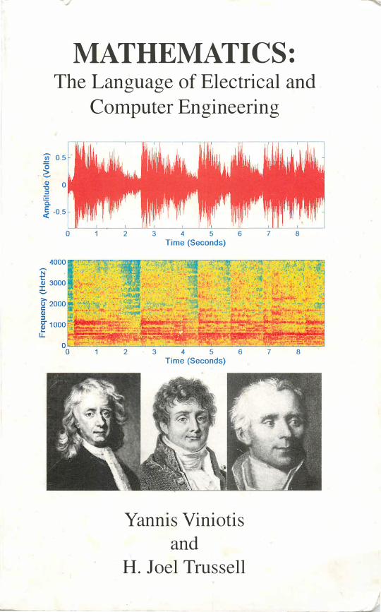
MATHEMATICS: The Language of Electrical and
Computer Engineering
2' 0.5
� � 0 � a. � -0.5
N � 3000 J: '-"
o 2
2
3 4 5 6 Time (Seconds)
3 4 5 6 Time (Seconds)
Yannis Viniotis and
H. Joel Trussell
7 8
7 8

Mathematics: The Language of ECE
© Copyright 2005 Yannis Viniotis. All rights reserved. No part of this publication may be reproduced, stored in a retrieval
system, or transmitted, in any form or by any means, electronic, mechanical, photocopying, recording, or otherwise, without the written prior permission of the author.
Note for Librarians: A cataloguing record for this book is available from Library and Archives Canada at www.collectionscanada.calamicus/index-e.html
ISBN 1-4120-6503-8
oft fGreeil.;;tl \l� Printed in Victoria: BC, Canada. Printed on paper with mi,limum 30% /'f!rycled fibre. Traffords print shop
runs on "green energy "from solar. wind and other environmentally-frimdly power sources.
lRAFIORD_ PUBLISHING Offices in Canada. USA. Ireland and UK
This book was published on-demand in cooperation with Trafford Publishing. On-demand publishing is a unique process and service of making a book available for retail sale to the
public taking advantage of on-demand manufacturing and Internet marketing. On-demand publishing includes promotions, retail sales, manufacturing, order fulfilment, accounting and
collecting royalties on behalf of the author.
Book sales for North America and international: Trafford Publishing. 6E-2333 Government St .•
Victoria, BC V8T 4P4 CANADA phone 250 383 6864 (toll-free I 888 232 4444 ) fax 250 383 6804; email to [email protected]
Book sales in Europe: Trafford Publishing (UK) Ltd., Enterprise House, Wistaston Road Business Centre,
Wistaston Road, Crewe, Cheshire CW27RP UNITED KINGDOM phone 01270 251396 (local rate 0845 230 9601) facsimile 01270 254 983; [email protected]
Order online at: trafford.com/03-1138
10 9 8 7 6 5 4 3 2 I
MATHEMATICS: THE LANGUAGE OF ELECTRICAL
AND
COMPUTER ENGINEERING Second Edition
YANNIS VINIOTIS Professor ECE Department NCSU Raleigh, NC, USA
H. JOEL TRUSSELL Professor ECE Department NCSU Raleigh, NC, USA
,-"

Contents
List of Figures List of Tables Preface Acknow ledgments Introduction What is the story ill this book?
1 . BACKGROUND CONCEPTS Real-valued functions
2
3
4
5
1 . 1 Functions of a single real or integer variable 1 .2 Uses of the function concept in ECE 1 .3 1 .4 1 .5
Mathematical operations on a function Odd and even functions Zeros of a function
Derivatives of a function 2 . 1 De L'Hospital's rule Integral of a function 3 . 1 Integration by change o f variables 3.2 Integration by parts The exponential function and its properties 4. 1 Derivatives of the exponential function 4.2 Integrals of the exponential function 4.3 Taylor series expansion of the exponential function 4.4 Useful properties of the exponential function The sinusoidal functions and their properties 5. I . Derivatives and integrals of the sinusoidal functions 5 .2 Taylor series expansion of the sinusoidal functions
v
xiii xix xxi xxv
xxvii
I 2 2 2 2
1 6 1 9 20 2 1 22 22 25 26 27 27 28 28 28 29 30
/

vi MATHEMATICS: THE LANGUAGE OF ECE
5.3 Useful properties of the sinusoidal functions 30 6 Algebraic Equations for straight lines 3 1
6. 1 The slope-intercept equation of a single line 3 1 6.2 Equations for multiple lines 3 1
7 Fraction expansions 3 1 8 Facts from trigonometry 33
8 . 1 The inverse tangent 34
2 . SIGNALS IN ENGINEERING 5 1 1 Pulse-shaped signals 53
1 . 1 The unit-step function u(t) 53 1 .2 The unit pulse signal 59 1 .3 The centered unit pulse signal 60 1 .4 The 8(t) function 60 1 .5 Clock generator signals 63
2 Sinusoidal signals 64 2 . 1 Parameters of sinusoidal signals 64 2.2 Operations on sinusoidal signals 66
3 Exponential signals 69 3 .1 Cosine times exponential signals 70
4 Periodic signals 70 4.1 The period of a signal 7 1 4.2 Approximations of periodic signals 77
5 Time shifting and scaling of signals 78 5 . 1 Time scaling i n real life 78 5.2 Time shifting in real life 78 5.3 Time shifting and scaling of pulse-shaped signals 80
6 Summary of main points 85
3 . MATLAB PROGRAMMING 1 1 3 1 Defining a signal in Matlab 1 1 3
1 . 1 Arrays in MatIab 1 1 5 2 Plotting 1 16
2. 1 Commands for two-dimensional plots 1 1 6 2.2 Examples of accurate and inaccurate plots 1 2 1 2.3 Plotting of periodic signals 1 24 2.4 Multiple plots 1 24
3 Numerical operations 1 28

Contents vii
3 . 1 Algebraic operators 1 28 3 .2 Logical operators 1 28
4 Input and output commands 1 29 4. 1 Input of data through the screen 1 29 4.2 Output of data to the screen 1 30 4.3 Output of data to a file 1 3 1 4.4 Input of data from a file 1 3 1
5 Repeating operations more than once 1 3 1 5 . 1 For loops 1 32 5 .2 While loops 1 33
6 Vectorized operations 1 34 7 Functions 1 38
7 . 1 A library of Matlab functions for signal generation 1 40
4. COMPLEX NUMBERS AND FUNCTIONS 1 69 1 Definition of a complex number 1 70 2 Cartesian and polar representations 1 74 3 Arithmetic Operations 1 77 4 Euler's identity 1 80
4.1 Exponential representation of complex numbers 1 83 4.2 Multiplication, division, inverses and roots 1 88
5 Matlab commands and examples 1 94 6 Complex functions 1 99
6. 1 Complex functions of an integer-valued variable n 200 6.2 Complex functions of a real-valued variable 209
7 Phasors and applications in circuit analysis 2 1 4 7 . 1 . Simple circuits with sinusoidal inputs 2 1 4 7.2 Phasor description of a sinusoidal signal 2 1 5 7.3 The input/output phasor relationship 2 1 7
8 Integrals of complex exponential functions 2 1 9 9 Summary of main points 222
5. VECTORS AND MATRICES 241 1 Vectors 24 1
1 . 1 Vector Operations 242 1 .2 Matlab commands for vector operations 247
2 Matrices 248 2. 1 Definitions 248

viii MATHEMATICS: THE LANGUAGE OF ECE
2.2 Special matrices 25 1 2.3 Matrix Operations 252 2.4 Matlab commands for matrix operations 258 2.5 Matrix inverse 260 2.6 Matlab commands for matrix operations 266
3 Applications of matrices in robotics and graphics 268 3 . 1 Rotation and translation in Robotics 269 3.2 Translation 270 3.3 Rotation and translation 270 3.4 Rotation and translation of graphs 272
4 Summary of main points 272
6. SYSTEMS OF LINEAR EQUATIONS 285 Definition and notation 286 1. 1 Overdetermined and underdetermined systems 288 1 .2 Consistent and Inconsistent Systems 290
2 Applications of linear systems of equations 29 1 2.1 Linear systems in game theory 29 1 2.2 Applications in analysis of circuits 293 2.3 Sensitivity analysis of circuits 296
3 Solution via Gaussian elimination 298 4 Matlab solutions of systems 302 5 Fitting curves to experimental data 304
5 . 1 Data interpolation 307 5 .2 Least squares curve fitting 3 1 0 5.3 Least square fit with a general polynomial 3 14 5 .4 Matlab commands for least square fit with a general
polynomial 3 1 6 6 Summary of main points 3 1 9
7. DIFFERENTIAL EQUATIONS 329 Differential equations in circuit theory 330 1. 1 RC circuits in series 33 1
2 Classification and properties of differential equations 333 2.1 Classification of differential equations 333 2.2 Properties of differential equations 335
3 First order differential equations 340 3 . 1 Complementary Solution 341 3.2 Particular solution 343
Contents IX
3.3 Total Solution 349 4 Second order differential equations 35 1
4. 1 Complementary Solution 352 4.2 Particular solution 359 4.3 Total Solution 365
5 Numerical solutions via Euler's method 367 5 . 1 First order differential equation 367 5.2 Second order differential equation 370 5.3 nth order differential equation 374 5 .4 Systems of differential equations 377
6 Numerical Matlab solutions 380 7 Summary of main points 383
8 . LAPLACE TRANSFORMS 399 I Definition and calculation of the transform 399 2 Properties 405
2. 1 Uniqueness 405 2.2 Linearity 405 2.3 Time-shifting 406 2.4 Time-scaling 408 2.5 Time-reversal 4 1 1 2.6 Derivatives 4 1 1
3 Solving differential equations with Laplace transforms 4 1 3 3 . 1 First order differential equations 4 14 3 .2 Second order differential equations 4 1 5
4 Partial fraction expansions 4 16 4. 1 Proper rational fractions without repeated roots 4 1 6 4.2 Calculation of v(t) from V(s) 4 17 4.3 Examples 4 19
5 Transfer functions 422 6 Matlab commands 424 7 Summary of main points 427
9. FOURIER SERIES 441 1 Three representations of the Fourier Series 442
1 . 1 Are the three approximations periodic signals? 446 1 .2 Conversions between the three series formats 447 1 .3 Examples 448
x MATHEMATICS: THE LANGUAGE OF ECE
2 Fourier series representation of some common signals 462 3 .The frequency and power spectrum of a signal 467
3 . 1 Definition 467 3.2 Plotting the frequency spectrum 468 3.3 The power spectrum 475 3 .4 Another view of a time signal 480
4 Properties 483 4. 1 Uniqueness 485 4.2 Linearity 485 4.3 Time-shifting 485 4.4 Time-scaling 487 4.5 Time-reversal 489 4.6 . Derivatives 492
5 Solving differential equations with Fourier series 494 6 Summary of main points 500
10. FOURIER TRANSFORMS 5 1 5
1 Introduction 5 1 5
2 3
4 5 6
1 . 1 Definition of the transform and spectrum 5 1 5 1 .2 Relationship to Laplace transform and Fourier series 5 1 7 Fourier transforms of common signals Properties 3 . 1 Uniqueness 3.2 Linearity 3.3 Time-shifting 3.4 Time-reversal 3.5 Time-scaling 3.6 Derivatives 3.7 Examples Solving differential equations with Fourier transforms Matlab commands for calculating Fourier transforms Summary of main points
5 1 9 523 523 524 524 525 526 527 527 536 539 540
1 1 . LIGHT READING FOR SERIOUS ENGINEERS 555 555 555 557 557 557
1 Operation and characterization of a disk drive 1 . 1 How does a disk work? 1 .2 Some technical questions 1 .3 The electrical motor of a disk 1 .4 Issues for techies

Contents
2
1 .5 1 .6 1 .7
The sad story of Sir Isaac Sir Isaac and disks Issues for humble ECE220 students
Summary of main points
xi
558 560 561 562
List of Figures
1 . 1 The function f(x) = sin3 (27r100x) . 3 l .2 The function g(x) = sin3 (27r100x) + a, a = 3. 4 l .3 The function g(x) = sin3 (27r100x) - a, a = 3. 4 1 .4 The function h(x) = a · sin3 (27r100x) , a = 3. 5 l .5 The function h(x) = a · sin3 (27r100x) , a = 1/3. 6 l .6 The function hI (x) = X + x2 . 7 1 .7 The function h2 (X) = x - x2 . 7 1 .8 The function hI(x) = X · x2 . 8 1 .9 The function h2 (X) = x/x2 . 9 1 . 1 0 The function g(x) = sin3 (27r100(x - xo) ) , Xo = 0.003. 1 0 1 . 1 1 The function g(x) = sin3 (27r100(x - xo) ) , Xo = -0.003. 10 1 . 1 2 The function g(x) = sin3 (27r100( -x) ) . 1 1 1 . 1 3 The function g(x) = ( - x f. 1 2 1 . 14 The function g(x) = (-x) + (_x)2 . 1 2 1 . 1 5 The function g(x) = f (3x) = 3x. 1 3 1 . 1 6 The function f(x) in Example 1 . 1 0. 14 1 . 1 7 The function g(x) = f(ax) , a = 3. 1 5 1 . 1 8 The function g(x) = f(ax) , a = 1/3. 1 7 1 . 1 9 The function f(t) = Aeat , A = 1 , a = l . 27 1 .20 The function f(t) = sin(t) . 29 1 .2 1 The trigonometric circle. 34 l .22 The function f(t) = cos3 (27r100t) . 38 1 .23 The function f(t) = t3 + t2 + t + l . 38 2. 1 The function u(t ) . 54 2.2 The function g(t) = u(t) + a, a = 3. 55
xiii
xiv
2.3 2.4 2.5 2.6
2.7 2 .8 2 .9 2. 1 0 2. 1 1 2. 1 2 2. 1 3 2. 1 4 2. 1 5 2 . 1 6 2. 1 7 2. 1 8 2 . 1 9 2.20 2.2 1 2.22 2 .23 2.24 2.25 2.26 2.27 3 . 1 3.2
3 .3
3 .4
3 .5
3 .6
MATHEMATICS: THE LANGUAGE OF ECE
The function get) = au(t) , a = 3. The function get) = u(t - to) , to = 3 . The function get) = u( -t) . The pulse with unit amplitude and duration to time units, to = 3. The centered unit pulse signal Pr(t) , with T = 1. The c5 (t) function. The clock generator signal , Pe (t) . How to read the parameters of the sine signal J(t ) . Addition of sinusoidal signals, same frequency. Multiplication of two sinusoidal signals. Time scaling of the sine signal . Decaying oscillations. Decaying oscillations. The signal h3 (t) in Example 2.22. Plot for an unknown signal . A periodic pulse signal . A periodic ramp signal . A periodic signal . The signal h(t) in Problem 2.39. Transmission line connecting a source to a load. How touch-tone phones dial " 1 ". The Bipolar Return-to-Zero (BRZ) code. The On-Off Keying (OOK) code. The Binary Phase Shift Keying (BPSK) code. The Frequency Shift Keying (FSK) code. Plot of the factorial function. Plot of the function J(t) = sin(t) , with an appropriate discretization step. Plot ofthe functionJ(t) = sin(t) , with an inappropriate discretization step. Plot of the function J(t) = sin(106t) , over an inappro-priate interval . Plot of the function J(t) = sin( 106t ) , over an appro-priate interval. Plotting three functions in three separate graphs, l ined up on top of each other.
55 56 57
59 60 6 1 63 65 67 68 69 70 7 1 8 1 92 92 93 93 96
1 00 1 03 1 06 1 07 1 08 1 1 0 1 1 9
1 2 1
1 22
1 23
1 23
1 25

List of Figures xv
3.7 Setting common axis scaling in separate plots. 1 27 3 .8 The periodic pulse and ramp signals in Example 3 .29. 14 1 3 .9 The triangular pulse and sinc signals in Example 3 .29. 142 3. 1 0 Analog t o Digital conversion for beginners. 148 3 . 1 1 The transfer characteristic of the amplifier in Problem
3.26. 1 57 3 . 1 2 The output y(t) in Problem 3.28. 1 60 3. 1 3 Typical motor responses. 1 67 4. 1 Various points (complex numbers) on the Cartesian plane.
1 7 1 4.2 Various points on the unit circle. 1 88 4.3 Various points (complex numbers) on the Cartesian plane.
1 96 4.4 Various points (complex numbers) on the Cartesian plane.
197 4.5 The z (n) sequence on the Cartesian plane. 200 4.6 Magnitude spectrum of z(n) . 20 1 4.7 Phase spectrum of z (n) . 202 4.8 Magnitude of f(n) = 3ejO.025nn + 3ejO.01 7nn. 205 4.9 Phase of f (n) = 3ejO.025nn + 3ejO.Ol77rn. 205 4. 1 0 Real part of f (n) = 3ejO.025nn + 3ejO.01 7nn. 206 4. 1 1 Imaginary part of f (n) = 3ejO.025nn + 3ejO.01 77rn. 206 4. 1 2 Magnitude spectrum of H (w) . 2 1 1 4. 1 3 Phase spectrum of H(w) . 2 1 1 4. 1 4 The DTFf in Problem 4.5 1 , N = 10. 2 14 4. 1 5 The impedance of a transmission line, magnitude. 235 4. 1 6 The impedance of a transmission line, phase. 236 5 . 1 Example of rotation and translation of an object b y ma-
trix multiplication. 273 5 .2 A square in the two-dimensional plane. 280 5 .3 Rotation of a typical object. 280 5 .4 Translation of a typical object. 28 1 5 .5 The circuit in Problem 5 .23. 282 5 .6 The circuit in Problem 5.24. 283 6. 1 A fun l inear system of equations. 286 6.2 A prototype router with many linear systems of equations. 294 6.3 A generic three-stage circuit. 295

xvi MATHEMATICS: THE LANGUAGE OF ECE
6.4 Effect of R4 variations on current h (t). 297 6.5 Effect of C variations on current h(t). 297 6.6 Current measurements, ideal case. 305 6.7 Current m.easurements, circuits class lab, 5/3 1 103, the
day after the party at wn<I>. 306 6.8 Current measurements, circuits class lab, 6/01103, the
day after the day after the party at wn<I>. (The TA forced us to redo the lab.) 307
6.9 The graph of the function h(a) = 13a + 4 1 . 3 1 2 6. 1 0 The graph of the function h(a) = 13a + 4 1 + 15a - 21. 3 1 2 6. 1 1 Least squares fitting with a straight line. 3 1 5 6. 1 2 Fitting data with a polynomial of degree 3 . 3 1 8 6. 1 3 Fitting data with a polynomial of degree 2. 3 1 9 6. 1 4 A resistive circuit. 327 7 . 1 An RC circuit in series. 33 1 7.2 The total solution in Example 7. l 6. 350 7.3 The total solution in Example 7. 17 . 35 1 7.4 Typical behavior of the complementary solution of a
second order differential equation. 355 7.5 Overdamped complementary solution. 357 7.6 Overdamped complementary solution. 358 7.7 The total solution in Equation 7.96. 368 7 .8 The total solution in Example 7.28. 37 1 7.9 The solution v (t) in Example 7.30. 374 7 . 1 0 The total solutions obtained via ode230. 382 7. 1 1 "Unusual" driving forces. 390 8. 1 The signal y(t) in Equation 8.23. 4 10 8.2 The signal v(t) in Equation 8 .50. 42 1 8.3 The signal v (t) in Problem 8.3. 428 8 .4 The signal v (t) in Problem 8.4. 429 8.5 The signal v (t) in Problem 8.8. 430 8.6 The op-amp circuit in Problem 8.23. 433 8.7 The op-amp circuit in Problem 8.24. 434 8.8 The op-amp circuit in Problem 8.25 . 435 8.9 The MIMO circuit in Problem 8.30. 438 9 . 1 Fourier approximations, N = 3 (top) and N = 5 (bot-
tom). 443

List of Figures
9.2 9.3 904 9.5 9.6 9.7 9.8 9.9 9. 1 0 9. 1 1 9. 1 2 9. 1 3
9. 1 4 9. 1 5 9. 1 6 9. 1 7 9. 1 8 9. 1 9 9.20 9.2 1 9.22
9.23 9.24 9.25 9.26 9 .27 9.28 9.29 1 0. 1 1 0.2 1 0.3 lOA
1 0.5 1 0.6
The signal s(t) in Equation 9.33. The signal s(t) in Equation 9.34. The signal s(t) in Example 9.5 . The signal s(t) in Example 9.6. The approximating signal s(t) in Example 9.9, N = 2 . The approximating signal s(t) in Example 9.9, N = 10. A periodic centered pulse. A periodic ramp, with period T = 2. Another periodic ramp, with period T = 2. The spectrum of s(t) = sin(27r]"ot) . The spectrum of s ( t) = sin(27r fat + (J) , (J = 7r / 4. The spectrum of s( t) = cos(27r fat + (J) , fa = 1000 Hz and (J = 7r / 4. The spectrum of Equation 9040. Spectrum plot, signal in Example 9.5 . Spectrum plot, signal in Exa:mple 9. 1 0. Spectrum plot, signal in Example 9. 1 1 . Power spectrum plot, signal in Example 9.5 . The spectrum of a diva's voice. The response plot of an equalizer device. The time-reversed periodic ramp, with period T = 2. A reversed and time-shifted periodic ramp, with period T = 2 and to = 0.5 . Plot of the particular solution. A periodic rectified sine. A periodic half-sine. The spectrum of the signal in Problem 9.32. The spectrum of the driving force vs (t) in Problem 9040. The DC to AC conversion circuit in Problem 9046. The switching waveform alternatives in Problem 9.46. The spectrum of the signal in Equation 10. 1 2 . The spectrum of the signal in Equation 10. 1 3 . The signal s(t) in Example 1 0.8 . The spectrum of S(w) = L [3 - ejw - 2e-j2w] . The spectrum of S(w) = e-j2Wsin�w). The signal v( t) in Example 1 0. 1 1 .
xvii
449 450 454 456 462 463 463 465 467 469 47 1
472 472 473 475 476 478 484 484 490
49 1 498 503 504 507 509 5 1 1 5 1 1 52 1 522 528 53 1
533 534

xviii MATHEMATICS: THE LANGUAGE OF ECE
1 0.7 The spectrum of the transform in Equation 10.42. 535 1 0.8 The signals in the time domain. 546 10.9 The Fourier transforms. 547 10. 1 0 Implementation of a first-order Butterworth filter. 549 1 0. 1 1 Implementation of a third-order Butterworth filter. 550 1 0. 1 2 The raised cosine Binary Phase Shift Keying (BPSK)
code. 552 I Ll A high-level model for a disk and disk parameters. 556

List of Tables
I. 1 Where the ECE220 material is needed. xxix 1.2 Relation to other ECE courses. xxix 1 . 1 Derivatives of common signals. 2 1 1 .2 Trigonometric numbers table. 33 2. 1 Touch-tone frequencies. 102 2.2 ASCII codes for some characters and symbols. 104 3 . 1 MatIab built-in functions. 1 40 3 .2 MatIab built-in signals . 140 6. 1 Generic tabulation of experimental data. 307 8. 1 Laplace transforms of common signals. 404 8.2 Properties of the Laplace transform. 4 1 3 1 0. 1 Fourier transforms of common signals. 523
xix

Preface
AVTO TO f3�(3AW aVaL ipaJ.LJ.LEVO UTa AiiAu;;a. Hopefully, the rest of the book will not be all Greek to you.
YANNIS VINIOTIS
JOEL TRUSSELL
RALEIGH, NC
SPRING 2005
xxi

This book is dedicated to CNN (Candice, Nora, and Natalie) , my wife Maria, my mother Despina, and my sister Dimitra.
Yannis Viniotis
This book is dedicated to Lynne.
Joel Trussell
xxiii
Acknowledgments
We would like to acknowledge the invaluable contributions of Dr. Baran, ECE Department, NCSU. We would also like to thank Mr. Frank Perry and Mr. Zhen Yuan for their help with Matlab scripts; Ms. Christine Strom, Ms. WenJun Li and Mr. Daniel Bruhn for their help with proofreading.
xxv

Introduction
What is the story in this book?
This book puts together mathematical concepts and techniques for applications in electrical and computer engineering. The presented concepts are sine qua non 1 in both describing and understanding electrical signals and their properties. The emphasis is placed on how a concept or technique is applied to an electrical engineering system, not on mathematical rigor. As a result, (most of) the existence/uniqueness questions that a typical mathematical textbook would raise and address are bypassed in this textbook.
Here are some (random) engineering questions that the various topics in this book will help you first understand and then answer. In parentheses, we list the relevant book topics.
I have only DC power available. Can I get an AC voltage out of it? How? (Fourier Series theory)
2 I want to send a file from one computer to another. What electrical signal is "best" for such a transmission? (Fourier Series , Fourier Transform theory)
3 Will a feedback system be stable? (Laplace Transform theory)
4 How do I make sure a motor does not oscillate wildly? (Differential Equations, Laplace Transform theory)
5 How do I sample an analog signal , like a sound, to store it in a computer efficiently? (Fourier Series, Fourier Transform theory)
6 How do I remove noise from a signal? (Fourier Series, Fourier Transform theory)
I Latin for essential
xxvii

xxviii MATHEMATICS: THE lANGUAGE OF ECE
7 I build a circuit with inaccurate components: how do I know the circuit will still meet specifications? (Linear Systems)
We will revisit these generic questions in later chapters, once we first develop, in sufficient detail, the language to both pose them and describe their answers.
In a nutshell , the logical sequence and dependence of the material presented in this book is the following: Chapter 2 introduces a few signals that are quite common in practice. The main purpose of this chapter is to introduce some basic operations of interest, such as time scaling, reversal and shifting. The time behavior of electrical systems (circuits being the major example) is described via differential equations (the subject of Chapter 7). Why such equations? Because of the presence of capacitors and/or inductors in an electrical system. Such equations involve a signal and its derivatives. The solution of a differential equation can be obtained either directly or through a transformation of the equation. Three such transforms are described in this book: Laplace, in Chapter 8; Fourier series, in Chapter 9 and Fourier transform, in Chapter 1 0. The three transforms provide for easy solutions of the differential equations ; more importantly, they provide a radically new way to interpret a signal (namely the frequency spectr.um concept, in Chapter 9, Section 3) . The language in which we describe transforms is that of complex numbers and functions, the material of Chapter 4. In electrical systems with more than one input and output (which is the majority of realistic systems), vectors and matrices, the material of Chapter 5, provide the natural language to describe them. In such systems, solving the equations that are the result of using vectors and matrices requires the material in Chapter 6.
Chapter 3 describes Matlab, the graphics and computation package we use throughout the book. While this chapter is "stand-alone", it is used in every other chapter to generate the figures and to solve the problems. This tool is one that we guarantee that you can use in every other electrical engineering course you take.
Finally, Chapter 1 collects all the "background" mathematical concepts and techniques we need to present the material in the remaining chapters. Ideally, you should have a high comfort level in every concept in this chapter.
Relation of the ECE220 material to other ECE courses
Table 1. 1 shows in detail in which ECE courses the material in each chapter will be used. Table 1.2 shows what specific topics from ECE220 other ECE courses will assume, as generic background.
Chapter organization
The techniques are illustrated with over two hundred and fifty examples; the examples usually immediately follow the material they are illustrating. Exam-

INTRODUCTION
II ECE220 chapter II ECE course that uses it
2 301.303.305.402,420,421.422,435.436,451.455.456
3 301,303.402.420.421.422,435,436,451,455.456
4 211,301,303.305,402,420,421,422.435,436,451,456
5 301,303,420,421,435.436.455
6 435,436,455
7 211,301,303,305,420,435,436.451.455,456
8 301.403.435.436.456
9 301,402.420.421,451
10 301,402,403,420,421,422,451
Table 1. 1 . Where the ECE220 material is needed.
II ECE course II main ECE220 topics needed
211 complex numbers, differential equations 301 signal operations. Matlab, complex numbers, matrices,
xxix
II
differential equations. Laplace transforms, Fourier series, Fourier transforms
303 signal operations, Matlab, complex numbers, matrices, differential equations
305 signal operations. complex numbers, differential equations 402 signal operations, Matlab, complex numbers,
Fourier series, Fourier transforms 403 Laplace transforms, Fourier transforms 420 signals operations, Matlab, complex numbers. matrices,
differential equations. Fourier series, Fourier transforms 421 signal operations, Matlab. complex numbers, matrices,
Fourier series, Fourier transforms 422 signal operations. Matlab. complex numbers. Fourier transforms 435 signal operations, Matlab, complex numbers, matrices,
l inear systems, differential equations, Laplace transforms 436 signal operations, Matlab; complex numbers, matrices,
l inear systems, differential equations. Laplace transforms 451 signal operations. Matlab. complex numbers,
differential equations, Fourier series. Fourier transforms 455 signal operations, Matlab, matrices, l inear systems,
differential equations 456 signal operations, Matlab, complex numbers,
differential equations, Laplace transforms
Table 1.2. Relation to other ECE courses.
II

xxx MATHEMATICS: THE LANGUAGE OF ECE
pIes marked with an asterisk are of a higher difficulty level . At the end of every chapter, the main points are summarized.
Over three hundred problems are given at the end of the chapters. Most of the problems are straightforward extensions of the examples in the text. Problems marked with an asterisk are either conceptually more difficult or lengthier. A few challenge problems require a deeper understanding of the material and the ability to put multiple concepts together. Finally, some of the problems, at the end of each problem section, are directly taken from other courses. These problems are intended to highlight the connection of the material in this book to topics you will encounter in the near future.
The provided Matlab scripts are ideal for concept reinforcement and visualization. Sometimes, a picture is worth a thousand words. Make sure you try these scripts out.
Prerequisites and assumption of students' background
Students are expected to have a good background and working experience in the following topics:
• Integral and differential calculus - finding the derivative and integral of given functions.
• Functions - performing simple algebraic operations on functions (e.g . , summation, multiplication).
• Graphing functions in rectangular and polar coordinates.
• Trigonometry - values of sines, cosines and tangents of given angles; simple trigonometric identities.
• Algebra - roots of an equation, expressions for a straight line, polynomials.
Chapter 1 summarizes all the prerequisite topics we will need.

Chapter 1
BACKGROUND CONCEPTS
This is what you should already know!
The material in this chapter summarizes all the mathematical concepts and techniques needed as background in later chapters. Section 1 introduces realvalued functions, a concept used extensively in chapters 2 and 7 through 10. Section 2 introduces the (first) derivative of a function, a concept that's heavily used in Chapter 7 . Section 3 introduces the integral of a function, a concept heavily used in chapters 8 through 10. Sections 4 and 5 summarize the properties of exponential and sinusoidal functions. These functions represent some of the most common signals we see in practice; they are heavily used in chapters 7 through 10. Section 6 reviews how straight lines can be represented via algebraic equations. A thorough understanding of this material is necessary for Chapter 6. Section 7 reviews expansion of fractions, a technique useful in Laplace transforms (Chapter 8). Finally, trigonometric numbers and concepts (especially that of the inverse tangent) are fundamental for a better understanding of complex numbers in Chapter 4. Throughout the chapter, we will note how each of these topics is related to real problems in electrical engineering.
2 MATHEMATICS: THE LANGUAGE OF ECE
1. Real-valued functions
1.1 Functions of a single real or integer variable
A real-valued function, f(x) , of a single real-valued variable, x (called the independent variable), is a mapping from the set of real numbers into the set of real numbers . (The mapping can also take complex values, as we will see later in Chapter 4.)
A real-valued function , f(x) , of a single integer-valued variable, x, i s a mapping from the set of integer numbers into the set of real numbers.
In electrical and computer engineering (ECE) applications, the independent variable x is often used to represent: (a) continuous time (in which case we often use the symbol t instead), (b) discrete time (in which case we often use the symbol n instead), (c) continuous frequency (in which case we often use the symbol w instead), or, (d) discrete frequency (in which case we often use the symbol n).
A function is represented via a mathematical formula (see, for example, Equation 1 . 1 , page 3 in Section 1 .3) or a graph (see, for example, Figure 1 .2, page 4 in Section 1 .3) .
1.2 Uses of the function concept in ECE
Functions are widely used in the ECE world. Arguably, the single most common application is to represent a signal . Signals appear, for example, in :
Circuit analysis; they are used to describe input and output voltages and currents.
2 Communications; they are used, for example, to describe the transmitted or received voltages or electric fields.
3 Digital signal processing; they are used, for example, to describe the discrete values obtained by the analog-to-digital converter (ADC).
4 Control systems, where they describe the reactions of one element of a system (e.g., mechanical speed) to another element (e.g. , electrical current).
5 Computer design; for example, they can describe the timing sequence produced by the internal circuits of clock generators.
1.3 Mathematical operations on a function
Functions can be manipulated in a number of different ways. The operations on a function that we will mostly be interested in, from the aspect of ECE applications, are summarized in this section.
The properties in sections 1 .3 . 1 through 1 .3 .4 represent rudimentary operations in signal processing. The properties in sections 1 .3 .5 through 1 .3 .7 are fundamental for the conceptual background needed in chapters 8, 9 and 1 0.

Background concepts 3
1.3.1 Addition of a constant to a function Consider a function f(x) and a real number a (called a constant). The new
function g(x) defined as:
g(x) = f(x) + a
is called the sum of the function f (x) and the constant a.
Note that addition of a positive number a shifts the entire graph of the function f (x) upwards by a, as Figure 1 .2 shows. Addition of a negative number a shifts the graph of the function f (x) downwards by a, as Figure 1 .3 shows.
Example 1.1. Let f(x) = sin3 (27rlOOx) . This function is shown in Figure 1 . 1 . Figure 1 .2 shows the function
g(x) = sin3 (27rlOOx) + 3
while figure 1 .3 shows the function
g(x) = sin3 (27rlOOx) - 3.
The function f(x) = sin3(2rt 1 00 x}
o�------��------��----���----��
-0.008 -0. 006 -0.004 -0.00 2 0.002 0.00 4 0.006 0.008 0.01
Figure 1 . 1 . The function f(x) = sin3 (27r lOOx) .
(1.1)

4
E 0>
MATHEMATICS: THE LANGUAGE OF ECE
The function g(x) = Sin3(21t 100 x)+3
91x)
fix)
'. '. _1� __ � __ � ____ ��� ____ L-__ -L ____ � __ -L�� __ �
-0.01 -0.006 -0.006 -0.004 -0.002 0.004 0.006 0.006
-1
x ->
Figure 1 .2. The function g(x) = sin3 (27rlOOx) + a, a = 3.
The function g(x) = sin3(21t 100 x)-3
fix)
........... :'
. " ..•
..........•
. ...-...-... �, , .. � �.
0.01
-5��������--��--������������ -0.01 -0.006 -0.006 -0.004 -0.002 0.002 0.004 0.006 0.006 0.01 X -->
Figure 1.3. The function g(x) = sin3 (27rlOOx) - a, a = 3.

Background concepts 5
1.3.2 Multiplication by a constant Consider a function f (x) and a constant a. The new function h( x) defined
as:
h(x) = af(x)
is the product of the function f (x) and the constant a. If l a l > 1 , the function h(x) is called an amplified version of f(x) . If
l a l < 1 , the function h(x) is called an attenuated version of f(x ) . Note that a can be positive or negative.
Example 1.2. Let f(x) = sin3 (2n100x) . Figure 1.4 shows the function
h(x) = 3 sin3 (2nlOOx)
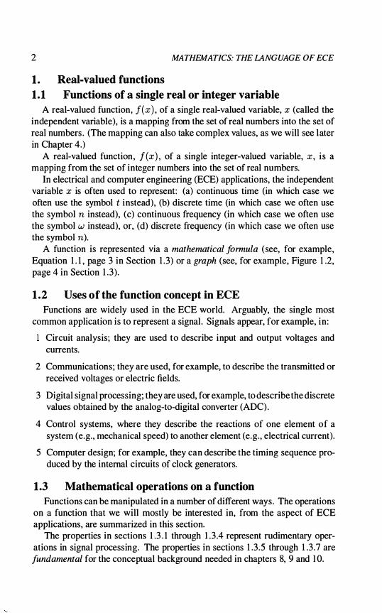
while Figure 1 .5 shows the function
h(x) = � sin3 (2nlOOx) .
The function h( x) ;: 3sin3( 2n 100 x)
_4'---'----'---'--:-'.,..,...---'----L.-..,.......---'---:'---' -0.01 -0.008 -0.006 -0.004 -0.002 0.002 0.00 4 0.006 0. 008 0. 01
Figure 104. The function h(x) = a · sin3 (27r lOOx) , a = 3.
6 MATHEMATICS: THE LANGUAGE OF ECE
The function h(x) = 1 /3 sin3(2x 100 x)
� � o��--� __ �--��+-c-�� __ ��--�� �
-1
-2
-3
:go':-:- 1-----:-o�.00::-8 ---::-0.=oos:----:-:0.0':-:04-----:-0�.00::-2 ---:---::-:0.0':-:02-----:0�.00::-:-4 ---=-O.=oo-=-s ---=-0.0:'::08,--------:-'0.01
x ->
Figure 1 .5. The function h(x) = a · sin3 (2rrlOOx) , a = 1/3.
1 .3.3 Addition and subtraction of functions Consider two functions f(x) and g(x) . The function
h(x) = f(x) + g(x)
is the (point-wise) addition of f(x) and g(x) . Subtraction is defined in a similar fashion.
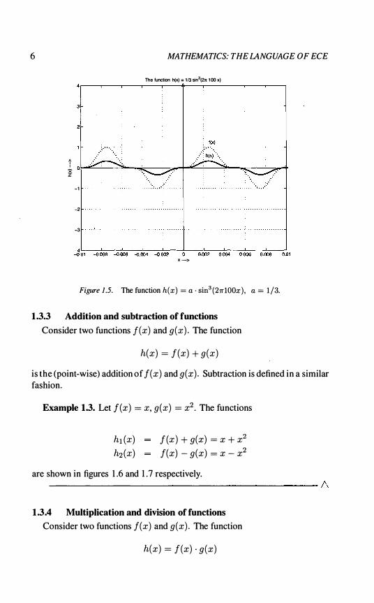
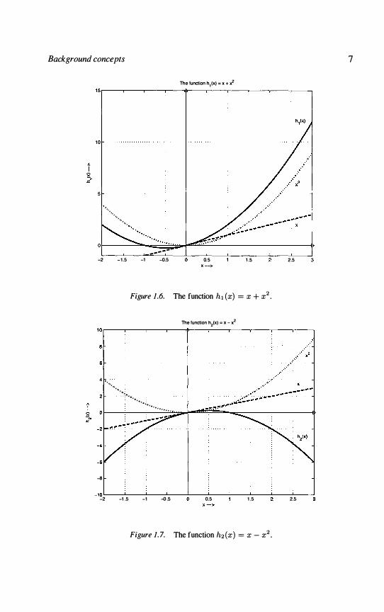
Example 1.3. Let f(x) = x, g(x) = x2 . The functions
hl (X) f (x) + g(x) = x + x2 h2 (X) f(x) - g(x) = x - x2
are shown in figures 1 .6 and 1 .7 respectively. --------------------------------------------- 6
1 .3.4 Multiplication and division of functions Consider two functions f(x) and g(x) . The function
h(x) = f(x) . g(x)
Background concepts
The function h1(x) = x + .; 15r---�----�--�----�---.----�----r---�----�---.
1 0
...... .........
-2 - 1 .5 .. ...... -
-1 -0.5 0.5 x -->
1 .5
Figure 1 .6. The function hi (x) = X + X2•
2.5
The function h2(X) = )( _ x2 1 0r---_.----,---�----�---.r_--_r----r_--_.----,_--_.
4 •.• , ...... ''';' .
.. : ..•.
•.
................
-8
_ 1 0 L-__ � ____ -L ____ � ____ L-__ -L ____ � ____ L-__ � ____ -L ____ � -2 -1.5 -1 -0.5 0.5 1 .5 2.5
Figure 1. 7. The function h2(x) = x - x2•
7
8 MATHEMATICS: THE LANGUAGE OF ECE
is the (point-wise) multiplication f(x) and g(x) . Division is defined in a similar fashion.
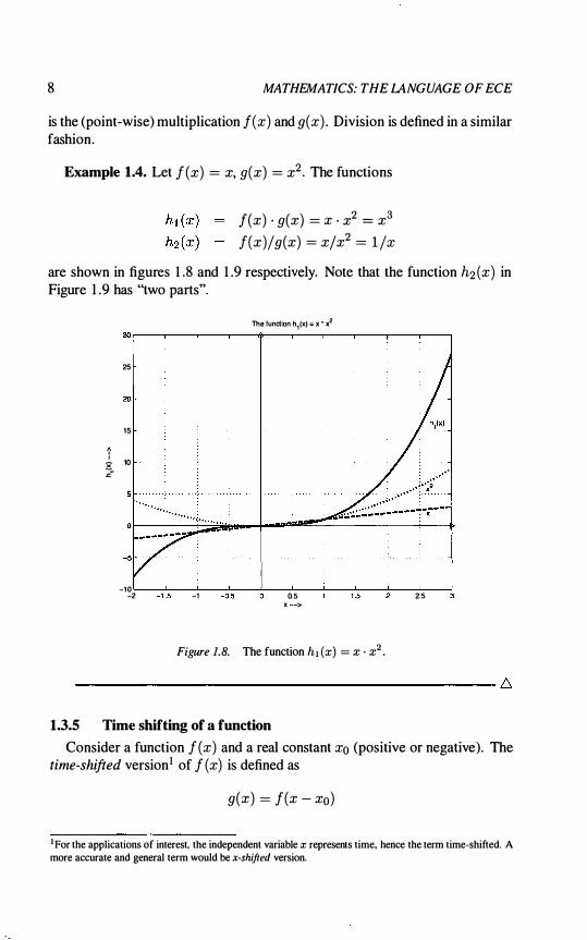
Example 1.4. Let f(x) = x, g(x) = x2 . The functions
f(x) · g(x) = x · x2 = x3
f(x)jg(x) = xjx2 = I jx
are shown in figures 1 .8 and 1 .9 respectively. Note that the function h2 (X) in Figure 1 .9 has "two parts".
The function h,(x):;: x • )(2
25
20
15
: � 10
-10 L-----:"':-_"'------::"':-_'--_'------"'----,',,---------"'-_'------' -2 -1.5 -1 -0 .5 0.5 1.5 2.5
x -->
Figure 1.B. The function h1{x) = X · X2.
1.3.5 Time shifting of a function Consider a function f (x) and a real constant Xo (positive or negative). The
time-shifted version 1 of f (x) is defined as
g(x) = f(x - xo)
I For the applications of interest, the independent variable x represents time, hence the term time-shifted. A more accurate and general term would be x-shifted version.

Background concepts
The function h2(X) ::: x I .j!-20r---'---�----.---�----.---'---�----.
15
10
••••• x2 ,,0'
J ��"�'''�'' ''�'' ''�''' '�'''� '''���������'�= ' �'=� ' �=' ' �� ' '��'��-
�N 0 ... ..... :.: .:.,:.:,: - - -" ,pt.", • • � ---- - - - -
x -5
-10
-15
-��--�--�----�--�----�--�--�--� -2 -1.5 -1 -0.5 0.5 1.5
x -->
Figure 1 .9. The function h2(X) = X/X2 .
9
If Xo is a positive number, the graph of the function f (x) is shifted to the right by Xo. If Xo is a negative number, the graph of the function f (x) is shifted to the left by Xo.
Example 1.5. Let f(x) = sin3 (27r100x) be the function shown in Figure 1 . 1 . Figure 1 . 10 shows the function
g(x) = f(x - 0.003) = sin3 (27rl00(x - 0.003 ) )
while Figure 1 . 1 1 shows the function
g(x) = f(x + 0.003) = sin3 (27rlOO(x + 0.003 ) ) .
1.3.6 Reversal of a function The reversed version of a function f (x) is defined as the new function
g(x) = f( -x)
The graph of g(x) i s the mirror image of the gntph of f (x) around the vertical axis. If the independent variable x represents time, the operation is

10
1.5
0.5
-0.5
-1.5
:/, ........ .
MATHEMATICS: THE LANGUAGE OF ECE
The function g(x) � 5in3(2.100 (x-0.003 ))
fIx) g(x)
�L-__ -L __ �� __ J-__ � ____ � __ -L ____ � __ -L ____ � __ � -0.01 -0.008 -0.006 -0.004 -0.002 0.002 0.004 0.006 0.008 0.01
x->
Figure 1 .10. The function g(x) = sin3 (27r100(x - xo) ) , xo = 0.003.
The function g(x) • 5in3(2.100 (x+0.003))
x 0;
-1.5
-2�����=-��--�=---����������=-� -0.01 -0.008 -0.006 -0.004 -0.002 0.002 0.004 0.006 0.008 am x->
Figure 1 . 1 1 . The function g(x) = sin3 (27r100(x - xo) ) , Xo = -0.003.
Background concepts 11
time reversal. This may sound like science fiction but we will encounter many practical uses for this operation.
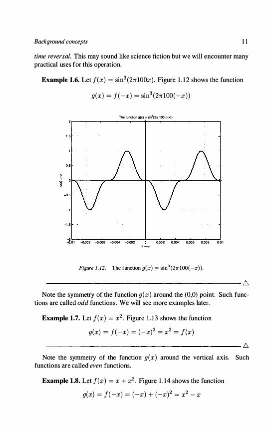
Example 1.6. Let f(x) = sin3 (27r100x) . Figure 1 .12 shows the function
g(x) = f(-x) = sin3 (27r100(-x) )
The function g( x) :;: sin3(2rc 100 ( -x))
1.5
-1.5
_2L----''------'_---'_--'-_-......l.._--'-_-'-_----'-_-'-_--l �.01 �.008 �.006 �.004 �.002 0.002 0.004 0.006 0.008 0.01
x -->
Figure 1. 12. The function g (x) = sin3 (21l"lOO( -x)).
---------------------------------------------- � Note the symmetry of the function g(x) around the (0,0) point. Such func
tions are called odd functions. We will see more examples later.
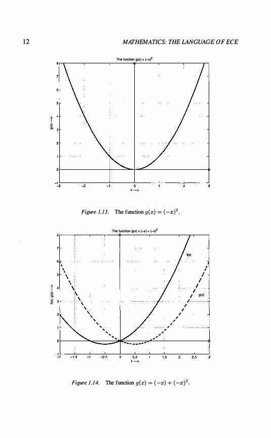
Example 1.7. Let f(x) = x2 . Figure 1 . 1 3 shows the function
g(x) = f( -x) = (_x)2 = x2 = f(x)
--------------------------------------------- � Note the symmetry of the function g(x) around the vertical axis. Such
functions are called even functions.
Example 1 .8. Let f(x) = x + x2 . Figure 1.14 shows the function
g(x) = f(-x) = (-x) + (-xf = x2 - X
12 MATHEMATICS: THE LANGUAGE OF ECE
The function g(x) = (_x)2
E '"
-�3�----�
_2�-----
_�1------�-------L------�----�
6
I 4 E '" g 3
\ \ \
'. .. ... \
\
x->
Figure 1. 13. The function g(x) = (_X)2.
The function g(x) = (-x) + (_x)2
. \ \
, , , , . . . , . .... . , ., . , ' .. ,,'
, ., .. , ,.
� , , I
I /
I . .... L
I I g(x)
I · I
-�2�--
-�1 .5�--
_71---
-�O. 75--
�--�O�.5���--
1�.5���--
2�.5�� x->
Figure 1 . 14. The function g(x) = (-x) + (_X)2.
Background concepts 13
as a dotted line, and the function f(x) as a solid line. Note that the function g(x) is neither odd nor even. ---------------------------------------------,. 6
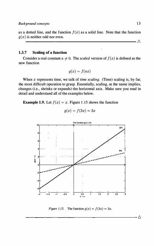
1.3.7 Scaling of a function Consider a real constant a 1- O. The scaled version of f(x) is defined as the
new function
g(x) = f(ax)
When x represents time, we talk of time scaling. (Time) scaling is, by far, the most difficult operation to grasp. Essentially, scaling, as the name implies, changes (i .e . , shrinks or expands) the horizontal axis . Make sure you read in detail and understand all of the examples below.
Example 1 .9. Let f(x) = x. Figure l . lS shows the function
g(x) = f(3x) = 3x
The function g(x) = 3x 1 0.---.---.---.---+---.---.---�--._--._--�
-2 -1 .5 -1 -0.5 0.5 x ->
1.5
Figure 1 .15. The function g(x) = f(3x) = 3x.
g(x)
2.5
14
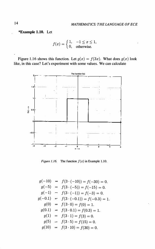
*Example 1 .10. Let
MATHEMATICS: THE LANGUAGE OF ECE
f(x) = {�: -1 ::S x ::S 1 , otherwise.
Figure 1 .16 shows this function. Let g(x) = f(3x) . What does g(x) look like, in this case? Let's experiment with some values. We can calculate
The function '(x)
1.5
� � 0.5 '"
O�----------�--r---�--------�
-0.5
-�L---_3�--_2�--_�1 ---0�--�--�--��· x -->
Figure 1.16. The function f(x) in Example 1.10.
g( - 10) g (-5) g( - 1)
g( -0. 1 ) g(O)
g(O . l ) g ( l ) g(5)
g( 10)
f (3 · (- 10) ) = f( -30) = O. = f(3 · (-5) ) = f(-15) = O.
f (3 · (-1 ) ) = f(-3) = 0. f(3 · (-0. 1 ) ) = f( -0.3) = 1 . f ( 3 . 0) = f(O) = 1 . f(3 · 0. 1 ) = f(0.3) = 1 .
= f(3 · 1 ) = f(3) = O. f(3 · 5) = f(15) = O. f(3 · 10) = f(30) = o.

Background concepts
In general ,
g(x) = f(3x) = {�: - 1 ::; 3x ::; 1 , otherwise.
or,
g(x) = {�: -1 /3 ::; x ::; 1/3, otherwise.
1 5
Figure 1 . 17 shows the function g(x) . A s we can see from this figure, multiplying the argument of the function by 3 "has shrunk " the graph of the function by a factor of 3. Even though it is not apparent, can you argue that the same shrinking occurred in Figure 1 . 1 5 ?
1 .5
I' _ 0.5 �
-0.5
1 -4
The function 9(X)=1(3x)
-r-
-3 -2 -1 x->
Figure 1. 1 7. The function g(x) = f(ax) , a = 3.
*Example 1.11. Let
f(x) = {�: - 1 ::; x ::; 1 , otherwise.
Let a = 1/3 and g(x) = f(ax) = f (!x) . What does g(x) look like, in this case? Let's again experiment with some values. We can calculate

16 MATHEMATICS: THE lANGUAGE OF ECE
In general ,
or,
g( - 10) g(-5) g( - 1 )
g ( -0. 1 ) g(O)
g(O. I ) g ( l ) g(5)
g( lO)
f( I/3 · (- 10) ) = f(-1O/3) = O. f(I/3 · (-5) ) = f( -5/3) = O. f( I/3 · (- 1 ) ) = f( - 1/3) = 1 . f(I/3 · (-0. 1 ) ) = f( -0. 1 /3) = 1 . f (I/3 · (0) ) = f(O) = 1 . f( I/3 · (0. 1 ) ) = f(0. 1/3) = 1 . f (I/3 · ( 1 ) ) = f(I/3) = 1 . f(I/3 · (5 ) ) = f(5/3) = O . f(I/3 · ( 10 ) ) = f( 1O/3) = O.
g(x) = f( I/3x) = {�: - 1 < Ix < 1 - 3 - , otherwise.
( ) { I , -3 ::; x ::; 3, 9 x = 0, otherwise.
Figure 1 . 18 shows the function g(x) . As we can see from this figure, multiplying the argument of the function by 113 "has expanded" the graph of the function by a factor of 3 = 1/ a. -------------------------------------------- 6
1.4 Odd and even functions
1 .4.1 Odd functions The function f (x) is odd if the following property holds true for every x:
f(x) = -f(-x) ( 1 .2)
The graph of an odd function is "anti-symmetric" around the (0,0) point. We can determine whether a given function is odd by either checking the
definition in Equation 1 .2 or verifying symmetry around the (0,0) point, once a graph of the function is given .
Example 1.12. The function in Figure 1 . 1 5 , page 1 3, is odd, since it is anti-symmetric around the (0,0) point. Alternatively,
f(x) = 3x = -3( -x) = -f( -x)

Background cOlicepts
The function g(x)=f(xI3)
1.5
7 � 0.5
-0.5
I � __ � __ � ____ L-__ � __ � ____ � __ -L __ � -4 -3 -2 -I
x ->
Figure 1 . 18. The function g(x) = f(ax), a = 1/3.
and the definition in Equation 1 .2 applies.
Example 1.13. Let k be any integer. The function
f(x) = x2k+ l
is odd, since
1 7
f( -x ) = (-xfk+l = (_x)2k . (-x) = x2k . ( -x) = _x2k+1 = -f(x) .
-------------------------------------------- 6
Example 1.14. The function
f(x) = sin(27TlOOx)
is odd, since
fe-x) = sin(27TlOO(-x) ) = - sin(27TlOOx) = -f(x) .
---------------------------------------------,- 6
18 MATHEMATICS: THE LANGUAGE OF ECE
Example 1.15. The function
f(x) = sin(27r100x + 7r/4)
i s not odd, since
f( -x) = sin(27r100( -x) + 7r/4) =I- - sin(27r100x + 7r/4) .
--------------------------------------------- 6
1.4.2 Even functions The function f (x) is even if the following property holds true for every x:
f(x) = f(-x) ( 1 .3)
The graph of an even function is symmetric around the vertical axis. We can detennine whether a given function is even by either checking the
definition in Equation 1 .3 or verifying symmetry around the vertical axis, once a graph of the function is given.
Example 1.16. The function in Figure 1 .16, page 14, is even, since it i s symmetric around the vertical axis. Alternatively, from its definition, we have that
f(-X) = {�: -1 ::; -x ::; 1 , otherwise.
or f( -x) = { 1 , - 1 ::; x ::; 1 ,
0, otherwise.
The last equation shows that f( -x) = f(x) and the definition in Equation 1 .3 applies. --------------------------------------------- 6
Example 1.17. Let k be any integer. The function
f(x) = x2k
is even, since
f(-x) = (_x)2k = x2k = f(x) .
--------------------------------------------- 6
Background concepts 1 9
Example 1.18. The function
f(x) = cos(2rrl00x)
is even, since
f( -x) = cos(2rrlOO( -x)) = cos(2rrl00x) = f(x) . ---------------------------------------------- 6
Example 1 .19. The function
f(x) = cos(2rrlOOx + rr/4)
is not even, since
f( -x) = cos(2rrl00( -x) + rr / 4) =1= cos(2rrlOOx + rr / 4) .
--------------------------------------------- 6 Odd and even functions appear frequently in Fourier series (see Chapter 9).
1.5 Zeros of a function
Consider a function f(x) . The real number Xo is called a zero o/the/unction f(x) if Xo satisfies the equation f(xo) = O. Note that Xo is also called a root 0/ the equation f (xo) = O. Throughout this text, we will use the terms zero of a function and root of a function interchangeably. Note that a function may have none, exactly one, mUltiple or an infinite number of zeros.
Example 1 .20. A polynomial of degree N has exactly N roots (some of which may be complex numbers). -------------------------------------------- 6
Example 1.21. The function f( x) = eX has no zeros, or, the equation eX = 0 has no roots. -------------------------------------------- 6
Example 1 .22. The function f (x) = sin( x) has an infinite number of zeros (roots) . The numbers Xo = 0, rr, -rr, 2rr, -2rr, and, in general, the numbers k7r, where k is any integer, all satisfy the equation f(x) = 0, since
sin(h) = O . ---------------------------------------------- 6
Example 1.23. The function shown in Figure 1 . 16, page 14, has an infinite number of zeros. All the real numbers outside the interval [- 1 , 1] are zeros. -------------------------------------------- 6
20 MATHEMATICS: THE LANGUAGE OF ECE
2. Derivatives of a function
The first derivative2 of the function f(x), denoted by f' (x) , is defined as the limit
f' ( ) - 1 ' f(x + h) - f(x)
x - lm ::"""':"--:-""-""::""':"""":'" h---+O h
Alternative notations for the first derivative are the following:
df(x) df f' ( ) f' dx ' dx ' x , .
We use them in the book interchangeably.
( 1 .4)
The first derivative of a function can be approximated via the difference
f' (x) � f (x + h) - f(x)
. h
( 1 .5)
In other words, we ignore the limiting operation in Equation 1 .4. Hopefully, whenever h is "small", the approximation in Equation 1 .5 is good. The approximation formula 1 .5 forms the basis for numerical solutions of differential equations, as we will see in Chapter 7, Section 5 .
Example 1.24. Let f(x) = 3x. We have
f' (x) = lim f(x + h) - f(x) =
lim 3 (x + h) - 3x h---+O h h---+O h
lim 3h = 3 h---+O h
On the other hand, the approximation in Equation 1 .5 gives us
f' (x) � f(x + h) - f(x)
h 3h
= 3 h
3 (x + h) - 3x h
and thus for this function the approximation introduces no error.
( 1 .6)
( 1 .7)
------------------------------------------- 6 Table 2 summarizes some common derivatives we will see in later chapters.
In this table, a is a real number.
2Derivatives are "everywhere" in an electrical engineers life: one source of this is the !Jbiquitous presence of capacitors! When a voltage v(t) is applied to these devices, they produce a current i (t) equal to
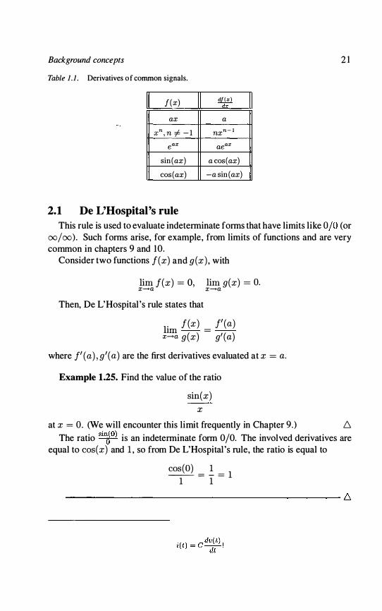
Background concepts
Table 1 . 1 . Derivatives of common signals.
" f(x)
ax
xn , n =Ie -1
e ax
sin(ax)
cos(ax)
2.1 De L'Hospital's rule
" df(x) -d-x
a
nxn- 1
aeax
a cos(ax)
-a sin (ax)
21
II
This rule is used to evaluate indetenninate fonns that have limits like % (or 00/(0). Such fonns arise, for example, from limits of functions and are very common in chapters 9 and 10.
Consider two functions f(x) and g(x) , with
lim f(x) = 0, lim g(x) = O. x�a x�a
Then, De L'Hospital 's rule states that
lim f(x) = J' (a) x-+a g(x) g' (a)
where J' (a) , g' (a) are the first derivatives evaluated at x = a.
Example 1.25. Find the value of the ratio
sin(x) x
at x = o. (We will encounter this limit frequently in Chapter 9.) 6 The ratio sindO) is an indetenninate fonn 0/0. The involved derivatives are
equal to cos(x) and 1 , so from De L'Hospital 's rule, the ratio is equal to
cos(O) 1 -- - - - 1
1 - 1 -

22 MATHEMATICS: THE LANGUAGE OF ECE
Example 1.26. Find the value of the ratio
at x = O. t::, The ratio s�n;6�) is also an indeterminate form 0/0. The involved derivatives
are equal to 2 sin(x) cos (x) and 67rx. The ratio is then equal to
2 sin(O) cos(O) 0 67r0 0
and we need to apply the rule once more. The new derivatives are 2 cos2 (x) -2 sin2 (x) and 67r, so finally
sin2 (0) 2 cos2 (0) - 2 sin2 (0) 1 37r02 67r 37r
-------------------------------------------- t::,
3. Integral of a function
Integrals are used frequently in the calculation of the transforms that we will present in chapters 8, 9 and 10. In evaluating such integrals, the two techniques we describe in this section are quite useful.
3.1 Integration by change of variables
Changing of the integration variable simplifies evaluation of certain integrals, as the following examples demonstrate.
Example 1.27. Consider a function f(x) . Let Xo be a given real-valued constant. Let
y(x) = f(x - xo)
denote a (time )-shifted version of the function f (x) . Suppose that the integral
D. jOO F(s) = -00 f(x)e-SXdx
has already been evaluated and thus the function F(s) is known. We want to evaluate the new integral
D. jOO Y(s) = -00 y(x)e-SXdx

Background concepts
We can write
Y(8) 6 L: y(x)e-SXdx = L: f(x - xo)e-SXdx
L: f(u)e-s(u+xO) du
L: f(u)e-SUe-sxodu
e-sxo L: f(u)e-SUdu
e-sxo L: f(x)e-SXdx
e-SXQ F(8)
23
( 1 .8)
0 .9)
In deriving Equation 1.8, we made the change of variables u = x - Xo . With this change,
• we can substitute u = x - Xo in the f(x - xo) tenn;
• we can substitute x = u + Xo in the e-sx tenn;
• we can substitute dx = d( u + xo) = du in the dx tenn;
• we can detennine the limits of integration with respect to the u variable as follows: for the lower limit, when x ---> -00, we also have u = x - Xo --->
-00. For the upper limit, when x ---> 00 , we also have u = x - Xo ---> 00.
So, finally, the function Y (8) can be evaluated without integration, directly from Equation 1 .9 . --------------------------------------------- 6
*Example 1.28. Let 8 be a known constant. Suppose that the integral 6 100 F(8) = -00 f(x)e-SXdx
has already been evaluated and thus the function F( 8) i s known. With this notation,
F( -8) = L: f(x)e-(-s)xdx = L: f(x)eSXdx
Consider for example the integral 6 100 G(8) = -00 f( -x)e-SXdx

24 MATHEMATICS: THE lANGUAGE OF ECE
The function G( s) can be found, in terms of the function F( s) , without evaluating the integral, via the change of variables u = -x. With this change, we have dx = -duo Moreover, when x = 00, u = -00; when x = -00, u = 00. Using these facts, we can write
G(s) = L: f( -x)e-SXdx
J�oo f(u)e-s(-u) (-du)
- J�oo f(u)e-(-s)udu
= L: f(u)e-(-s)udu
F(-s)
In deriving Equation 1 . 10 we used the known property of integrals :
lb g(x)dx = - ia g(x)dx
*Example 1.29. Consider now the integral
G(s) � 1000 f(ax)e-SXdx
( 1 . 1 0)
where a > 0 is a given constant. The function G( s) can also be found, in terms of the function F( s) , without evaluating the integral , via the change of variables u = ax. With this change, we have dx = �du. Moreover, when x = 0, u = 0; when x = 00, u = 00. Using these facts, we can write
G(s) = 1000 f(ax)e-SXdx
1000 f(u)e-s(u/a) (du/a)
� roo f(u)e-(s/a)udu a Jo 1
= -F(s/a) a ------------------------------------------- 6
We will revisit and use these examples when we discuss the time-shifting, time-reversal and time-scaling properties of the Laplace and Fourier transforms, in chapters 8, 9 and 1 0.
Background concepts 25
3.2 Integration by parts
Integration by parts is a useful technique when integrating "complicated" functions.
Consider the derivative of the product of two functions f(t) and g(t) . We can write
df(t)g(t) = f(t) dg(t) (t)
df (t) dt dt + 9 dt
Integrating the above expression we can write
f(t)g(t) = J f(t)dg(t) + J g(t)df(t)
Rearranging terms in the above expression we get:
J f(t)dg(t) = f(t)g(t) - J g(t)df (t) ( 1 . 1 1 )
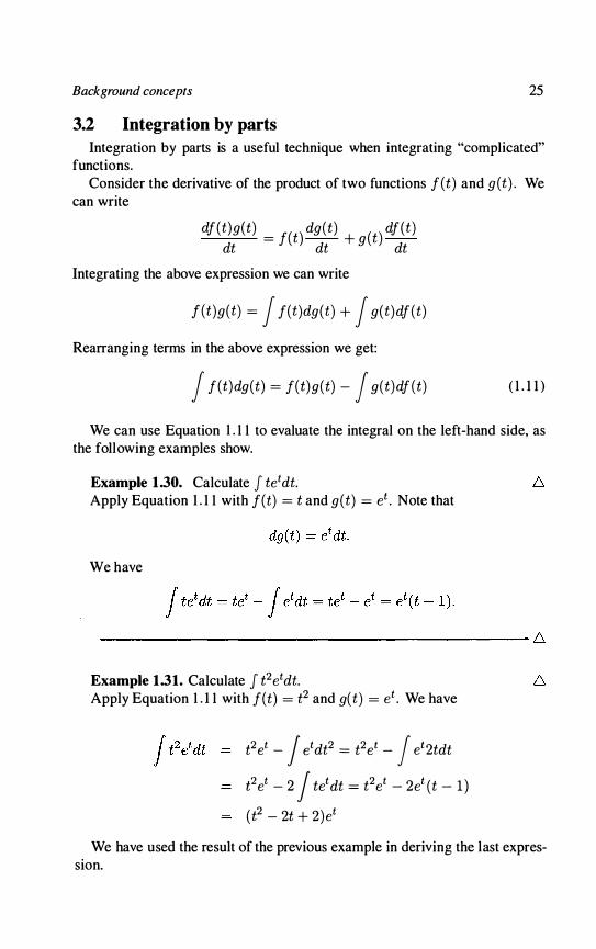
We can use Equation 1 . 1 1 to evaluate the integral on the left-hand side, as the following examples show.
Example 1 .30. Calculate J teldt. Apply Equation 1 . 1 1 with f(t) = t and g(t) = et . Note that
We have
-------------------------------------------- �
Example 1 .31. Calculate J t2etdt. Apply Equation 1 . 1 1 with f( t) = t2 and g( t) = et . We have
t2et - J etdt2 = t2et - J et2tdt
eet - 2 J tetdt = t2et - 2et (t - 1 )
(t2 - 2t + 2)et
We have used the result of the previous example in deriving the last expression.
26 MATHEMATICS: THE LANGUAGE OF ECE
Example 1.32. Calculate J t sin(t)dt. f:::, Apply Equation 1 . 1 1 with f(t) = t and g(t) = - cos(t) . Note that dg(t) =
sin(t)dt. We have then
J t sin(t)dt = - J td cos(t) = - [t cos(t) -J cos(t)dt] = -t cos(t) + sin(t)
------------------------------------------- f:::,
Example 1.33. Calculate J sin(t)etdt. f:::, Apply Equation 1 . 1 1 with f(t) = sin(t) and g(t) = et . Since dg(t) = etdt,
we can write
J sin(t)det = sin(t)et - J etd sin(t) = sin(t)et - J et cos(t)dt. (1 . 12)
Let's evaluate now J et cos(t)dt. Apply Equation 1 . 1 1 with f(t) = cos(t) and g (t) = et . Since dg(t) = etdt, we can write
J cos(t)det = cos(t)et - J etd cos(t)
cos(t)et + J et sin(t)dt . 0 . 1 3)
From Equations 1 . 12 and 1 . 1 3 we can write
J sin(t)etdt = sin(t)et - cos(t)et - J et sin(t)dt
and thus
J sin(t)etdt = � [sin(t) - cos(t)]
4. The exponential function and its properties
The function3
f(t) = Aeat , t E (-00, 00) ( 1 . 14)
is called the exponential function with parameters A, a (both real numbers).
3Note that we change the notation for the independent variable from x to t in this section and the next.

Background concepts 27
The parameter A is called the amplitude; we can easily check that A is the value of the function when t = O. Note that when t = - lla, J (t ) = Ae-1 = AI e. The special value t = - 1 I a is called the time constant.
A graph of this function for A = 1 , a = 1 is shown in Figure 1 . 1 9. ·Note that the function takes only positive values; it approaches 0 when t --> - 00 , and it "explodes" to infinity when t --> 00 .
ro.---�---.----.----'----.----.----r---�
60
50
40
20
10
-4 -3 -2
Figure 1. 19. The function f{t} = Aeat , A = 1, a = 1.
4.1 Derivatives of the exponential function
From Equation 1 . 1 4 we can easily see that
!, (t) = Aaeat , t E (- 00 , 00 ) and in general , for the n-th derivative,
4.2 Integrals of the exponential function
The (indefinite) integral of the exponential function is equal to
( 1 . 1 5 )
( 1 . 1 6)
28 MATHEMATICS: THE LANGUAGE OF ECE
This fact can be easily verified by differentiation of both sides of Equation 1 . 1 6. Moreover,
( 1 . 1 7)
This result is a simple extension of Example 1 .30.
4.3 Taylor series expansion of the exponential function
The Taylor series expansion of the exponential function is given by
(at) l (at)2 (at)3 1 + -- + -- + -- + · · · I ! 2! 3! f (at)k
k=O k!
4.4 Useful properties of the exponential function
( 1 . 1 8)
For any real (or complex) numbers a, b and n, the foIl owing properties are true:
eatebt (eatf
( eatr 1
e(a+b)t eant
1 -at - = e eat
5. The sinusoidal functions and their properties
The function
f(t) = A sin(wot + O) , t E ( - 00 , 00) is caIled the sine function with parameters A, Wo , O.
The function
g(t) = A cos(wot + 0) , t E (-00, 00 ) is caIled the cosine function with parameters A, wo , O.
( 1 . 1 9)
( 1 .20)
The parameter A is caIled the amplitude; we can easily check that A is the maximum value of the function. Wo is called the angular frequency. Sometimes
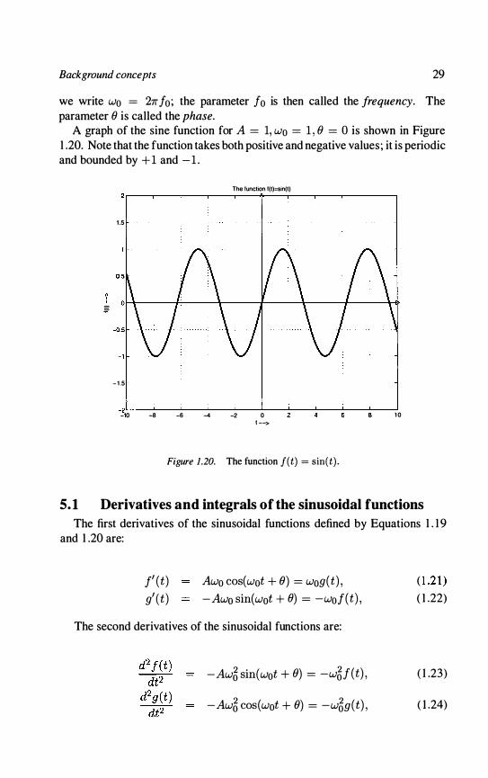
Background concepts 29
we write Wo = 211" fo; the parameter fo is then called the frequency. The parameter e is called the phase.
A graph of the sine function for A = 1, Wo = 1 , () = 0 is shown in Figure 1 .20. Note that the function takes both positive and negative values ; it is periodic and bounded by + 1 and -1 .
The function f(t)::sin(t)
1.5
- 1 .5
-2'---'---'-----'-----'---'----'----'----'----'----' -10 -8 -6 -4 -2 0 1 0
t -->
Figure 1.20. The function f(t} = sin(t } .
5.1 Derivatives and integrals of the sinusoidal functions
The first derivatives of the sinusoidal functions defined by Equations 1 . 1 9 and 1 .20 are:
f' (t) g' (t )
Awo cos(wot + e) = wOg(t) , -Awo sin(wot + 8) = -wof(t) ,
The second derivatives of the sinusoidal functions are:
-Aw6 sin(wot + 8) = -w6f(t) ,
-Aw6 cos(wot + e) = -w69(t) ,
( 1 .2 1 ) ( 1 .22)
0 .23)
( 1 .24)
30 MATHEMATICS: THE LANGUAGE OF ECE
The integrals of the sinusoidal functions are:
J f(t)dt
J g(t)dt
1 --g(t) Wo
�f(t) Wo
5.2 Taylor series expansion of the sinusoidal functions
The Taylor series expansions of the sinusoidal functions are given by
sin(at)
cos (at)
(at) l (at)3 (at)5 -- - -- + -- - . . . I ! 3! 5! 00
k (at)2k+ l E( -1) (2k + I ) ! (at)2 (at)4 (at)6 1 - -- + -- - -- + · · · 2! 4! 6!
00 ( )2k L)-l )k� k=O (2k) !
In the above expressions, a is any real number.
5.3 Useful properties of the sinusoidal functions
( 1 .25)
( 1 .26)
( 1 .27)
( 1 .28)
The following properties of the sinusoidal functions will be frequently used throughout this book.
In the following, a, b, a and (3 are arbitrary real numbers.
cos( -a) cos(a) sin( -a) - sin(a)
cos(a ± 7r/2) � sin(a) ( 1 .29) sin(a ± 7r/2 ) ± cos(a)
cos(a ± 7r) - cos(a) sin(a ± 7r) - sin(a) sin(a ± (3) sin(a) cos({3) ± cos(a) sin({3) cos(a ± (3) cos(a) cos({3) � sin(a) sin({3)
a cos(a) + b sin(a) J a2 + b2 cos(a - arctan(b/a) ) ( 1 .30)
cos(a) cos({3) 1 "2 [cos(a - (3) + cos(a + (3)] ( 1 .3 1 )

Background concepts 3 1
sin( a) sin(f3) 1 :2 [cos(a - 13) - cos(a + 13)] ( 1 .32)
sin( a) cos(f3) � [sin(a - 13) + sin(a + 13)] ( 1 .33)
6. Algebraic Equations for straight lines
6.1 The slope-intercept equation of a single line
The equation y = ax + b
represents the graph of a straight line in the (x, y) plane. The slope of the line is equal to a. The graph of the line intersects the y axis at the point (x, y) = (0, b) . It intersects the x axis at the point (x, y) = (-b/a, 0) .
The equation for a horizontal line (i .e. , a line with a slope of 0), that intersects the y axis at the point (x, y) = (0, b) is
y = O · x + b = b
The equation for a vertical line (i.e. , a line with a slope of 00), that intersects the x axis at the point (x, y) = (c, O) is
x = c
6.2 Equations for multiple lines
Consider the equations for two lines
Y a 1X + b1 y a2X + b2
The two lines are parallel if they have the same slope, i .e . , if a1 = a2 . Whenever a 1 ¥= a2 , the two lines will intersect each other. We will consider how to obtain the intersection point in Chapter 6.
7. Fraction expansions
Consider two polynomials in the variable4 s, denoted by N(s) and D(s ) . D (s) is in a product of factors form:
D(s) = (s + Sl ) (S + S2 ) . . . (s + sn )
The degree of D (s) is n. Assume that the degree of N (s) is less than n . Moreover, assume that the roots -Sl , -S2 , . . . , -Sn , are all distinct.
4The variable s is the symbol of choice in Chapter 8, where fraction expansions are used.
32 MATHEMATICS: THE LANGUAGE OF ECE
Fractions of the fonn N(s)/D(s) appear frequently in Chapter 8. Such fractions can always be simplified as a sum of fractions of the fonn:
N(s) Al A2 An -- = -- + -- + . . . + -D(s) S + SI S + S2 s + sn
regardless of the degree of N(s) (as long as it is less than n) . The following example demonstrates how to find the simpler fractions.
Example 1.34. Let
N(s) D(s)
3s + 2 (s + 5) (s + 3)
We can rewrite the fraction as
N(s) A B -- = -- + --D(s) s + 5 s + 3
( 1 .34)
( 1 .35)
where A and B can be found by equating the right -hand sides of equations 1 .34 and 1 .35.
3s + 2 (s + 5) (s + 3)
and thus
=
A B -- + --s + 5 s + 3 A(s + 3) + B(s + 5)
(s + 5) (s + 3) (A + B)s + 3A + 5B
(s + 5 ) ( s + 3)
3s + 2 (A + B)s + 3A + 5B (s + 5) (s + 3) (s + 5) (s + 3)
Since the denominators are equal, we must have
3s + 2 = (A + B)s + 3A + 5B
Note that the last equation must hold true for all values of s . The only way for that to happen is to have
A + B = 3, 3A + 5B = 2
from which A = 6 .5 and B = -3.5 . -------------------------------------------,- �
This method can be extended to any order polynomial . A polynomial of order n yields a linear system with n equations and n unknowns.

Background concepts 33
8. Facts from trigonometry
Angles are typically measured in degrees or radians. To convert the measure of an angle ()O in degrees to a measure ()rad in radians, and vice versa, we use
The trigonometric numbers of the angles in Table 8 are frequently used in examples and problems throughout chapters 4, 8, 9 and 1 0.
Table 1.2. Trigonometric numbers table.
8 (degrees) I 8 (radians)
0° 0
15° " 12 30° " "6 45° " 4" 60° " :i" 75° 5" 12 90° " 2"
sin( 8)
0 - 1"7f1 2 2
1 2 -jz �3 �
1 +.L3 2;:/2 1
cos(8) tan(8)
1 0 1 +.L3 272 2 - V3 �3 :73 2 J2 1 1 V3 2
- 1 +�3 272 2 + V3
0 undefined (±oo) ° ° " I I 90 < () < 180 I 2" < 8 < 1f I sm(1f - 8) I - cos(1f - ()) I - tan(1f - 8) I I
105° 7" 1 +.L3 \11 -2 + V3 12 2 72 120° 2" � 1 -V3 """ - ? 135° :E' -jz - -jz - 1 4 150° 5" 1 -:!i3 - � "6 2 165° l l 7r � _ 1+-j.f -2 - V3 "12 2h 2 2 180° 1f 0 - 1 0
- -
195° 13" 1 -.L3 1+ .L3 2 - V3 "12 272 - 2;:/2 210° 7" 1 -�l 1 "6 - 2 ;;3 225° "" - 72 1 "4 - 72 240° ¥ -� I V3 - :) 255° 17" .!.b'1 � 2 + V3 "12 - 272 - 2"2f 270° :1." - 1 0 undefined (±oo) .)
° ° I I 270 < () < 360 I �; < () < 21f I - sm(21f - ()) I cos(21f - ()) I - tan(21f - ()) I I - -
285° 19" - 1;ff � -2 + V3 "12 272 300° 7" - � 1 -V3 fi ? 315° " - :72 V'2 - 1 "4 330° l l 7r 1 ::/...3 1 6"" - 2 2 - ;;3 345° 23" - 1�3 I +ff 2 - V3 "12 2 2 2 2
34 MATHEMATICS: THE LANGUAGE OF ECE
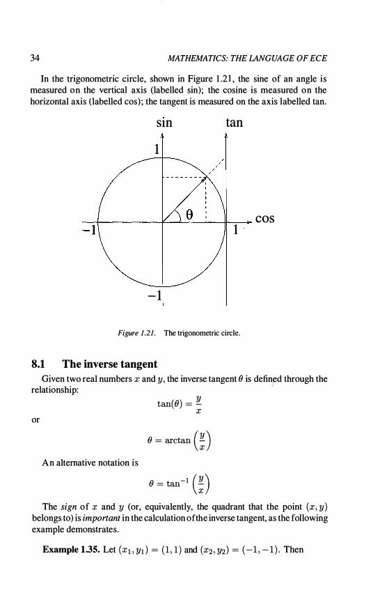
In the trigonometric circle, shown in Figure 1.2 1 , the sine of an angle is measured on the vertical axis (labelled sin); the cosine is measured on the horizontal axis (labelled cos) ; the tangent is measured on the axis labelled tan.
SIn tan
1
�+-�����-L���� ___ COS - 1 1
- 1
Figure 1.21. The trigonometric circle.
8.1 The inverse tangent
Given two real numbers x and y, the inverse tangent {} is defin�d through the relationship:
'
tan({}) = � x
or
e = arctan (;) An alternative notation is
e = tan-l (;) The sign of x and y (or, equivalently, the quadrant that the point (x, y)
belongs to) is important in the calculation of the inverse tangent, as the following example demonstrates.
Example 1 .35. Let (Xl , YI ) = ( 1 , 1 ) and (X2 , Y2 ) = (- 1 , - 1 ) . Then
Background concepts 35
(it = arctan (�: ) = arctan (�) = arctan ( 1 ) = 45°
and
(h = arctan (��) = arctan ( =� ) = arctan ( 1 ) = 45° + 180°
Even though in the argument of the arctanO function we have a 1 in both cases, (XI , Yl ) = ( 1 , 1 ) belongs to the first quadrant and (X2 ' Y2 ) = ( - 1 , - 1) belongs to the third one.
--------------------------------------------- 6
36 MATHEMATICS: THE LANGUAGE OF ECE
Problems
The concept of a function.
1.1. Sketch the following functions for t E [-10, 10] by hancP . From the sketch, detennine:
• The maximum value of the function in the interval [-10, 10] ; the value(s) of t for which the maximum occurs.
• The minimum value of the function in the interval [- 10 , 10] ; the value(s) of t for which the minimum occurs .
• The zero(s), if any, of the function in the interval [-10, 10] .
8S (t) t ( 1 .36) 8g (t) t + 3 ( 1 .37)
810 ( t) -3t ( 1 .38) 812 (t) min(3 , t) ( 1 .39) 813 (t) min( -3, t) ( 1.40)
814 (t) = 5 min(3, t) (1 .41 ) 815 (t) max(3, t) ( 1 .42) 816 (t) max(-3, t) ( 1 .43) 817 (t) 5 max(3, t) ( 1 .44)
You can use the sketches to see the answers to the following questions, but you need to show that the answers are correct mathematically.
1 Is 817 (t) 2: 814 (t) for all t E [-10, 1O] ?
2 Is 816 (t) 2: 813 (t) for all t E [- 10, 10] ?
Odd and even functions.
1.2. Let f(t) = lit . Show that this function is odd, i .e. , it satisfies the property in Equation 1 .2, page 1 6.
1.3. Let f(t) = 31t2 . Show that this function is even, i .e . , it satisfies the property in Equation 1 .3 , page 1 8 .
5It is important that you do the hand calculations, so that you develop some intuition about the functions.
Background concepts 37
1.4. Define and/or sketch an odd function of your own.
1.5. Define and/or sketch an even function of your own.
1.6. Let fo(t) be an odd function and fe et) be an even function. Show that the function
get) = fo(t) . fe (t)
is odd.
1.7. Let fo(t) be an odd function. Show that fo(O) = o. Hint: Let t = 0 in Equation 1 .2, page 1 6.
1.8. Let fo (t) be an odd function. Is the function
get) = fo(t) . fo (t)
odd, even or neither?
1.9. Let fe (t) be an even function. Is the function
get) = fe (t) . fe (t)
odd, even or neither?
1.10. Let fe (t) be an even function. Is the function
get) = fe et) + fe et)
odd, even or neither?
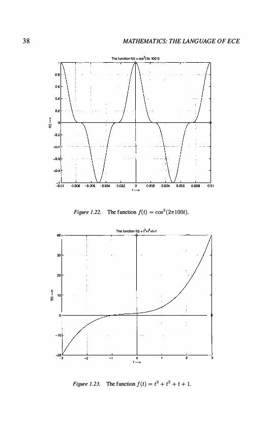
1.11. Consider the function shown in Figure 1 .22. Is this function odd, even or neither?
1.12. Consider the function shown in Figure 1 .23. Is this function odd, even or neither?
1.13. Can a function f(t) be both odd and even at the same time?
Derivatives of a function
1.14. In this problem, k is a positive integer and a is a real number. To avoid trivial ities, assume that a t= O. Find the following derivatives:
38
g
MATHEMATICS: THE LANGUAGE OF ECE
The function I(t) = cos3(2n 100 t)
t -->
Figure 1 .22. The function I(t) = cos3 (27rlOOt) .
The function 1(1) = 13 +� +t+ 1 �r-------.-------.-------+-------'-------.-------,
30
20
10
-10
���------��------_L1 -------7------�-------7------�
t -->
Figure 1.23. The function I(t) = t3 + t2 + t + 1 .

Background concepts 39
h(t) de-t dt
h(t) dtk -dt
f6 (t) d sin(t)
dt
h(t) d cos(t)
dt
fs (t) d sin(at)
dt
f9 (t) d cos(at)
dt
ho(t) dmin(3 , t)
dt
1.15. The first and second derivatives of the function f (t) are defined via the following limit expressions (whenever the limits exist) :
df(t) dt
d2 f(t) -----;I(2
1. f(t + h) - f(t) 1m -'--'-_-'------'-....;....c.
h-O h df(t+h) df(t )
lim -d-t - - (If"" h-O h
( l .45)
( 1 .46)
Let f(t) = bt . Use Equation 1 .45 to show that the first derivative is equal to b.
2 Let f (t) = -5t. Use Equation 1 .45 to show that the first derivative is equal to -5.
3 Let f(t) = t2 . Use Equation 1 .45 to show that the first derivative is equal to 2t.
4 Let f( t) = et . Use Equation 1 .45 to show that the first derivative is equal to et . (Hint: you will need to use De L'Hospital 's rule here.)
5 Let f(t) = t . Use Equation 1 .46 to show that the second derivative is equal to O.
6 Let f(t) = -5t. Use Equation 1 .46 to show that the second derivative is equal to O.
7 Let f (t) = t2 . Use Equation 1 .46 to show that the second derivative is equal to 2.

40 MATHEMATICS: THE LANGUAGE OF ECE
8 Let f(t) = et . Use Equation 1 .46 to show that the second derivative is equal to et . (Hint: you will need to use De L' Hospital 's rule here.)
1.16. Use De L'Hospital 's rule to find f (O) , where
f(t) = 1 - cos(t)
2t
1.17. Use De L'Hospital 's rule to find f ( 1O) , where
f(t) = 1 - cos(t - 10)
2t - 20
Definite and indefinite integrals
1.1S. In this problem, k is a positive integer and a is a real number. Find the following indefinite integrals :
f(t) J eSds
f(t) = J e5sds
f(t) J e-sds
f(t) J e-5sds
f( t) J skds
f(t) = J sin(s)ds
f(t) J cos(s)ds
f(t ) J sin(as)ds
f(t) J cos(as)ds
f(t) J sin(as) cos(as)ds
1.19. In this problem, k is a positive integer and a is a real number. T is a positive real number. Find the following definite integrals :
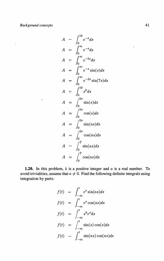
Background concepts 4 1
A 110 o e-sds
A 1000 e-sds
A 1000 e-5sds
A 1000 e-s sin(s)ds
A fo'X! e-3s sin(7s)ds
A 110 o skds
A 12� o sin(s)ds
A 12� o cos(s)ds
A 12� o sin(as)ds
A 12� o cos(as)ds
A loT sin(as)ds
A loT cos( as )ds
1.20. In this problem, k is a positive integer and a is a real number. To avoid trivialities, assume that a =f O. Find the following definite integrals using integration by parts:
f(t) jt -00 eS sin( as )ds
f(t) J�oo eS cos( as )ds
f(t) J�oo skesds
f(t) [00 sin(s) cos(s)ds
f(t) J�oo sin(as) cos(as)ds

42 MATHEMATICS: THE LANGUAGE OF ECE
1.21. In this problem, k is a positive integer and a is a real number. To avoid trivialities, assume that a f= O. Find the following definite integrals using integration by parts:
A 1000
e-s sin(as)ds
A 1000
e-s cos(as)ds
A 1000
s3 e -8 ds
A 102� o sin(s) cos(s)ds
A 102� o sin( as) cos( as )ds
1.22. Definite integrals of odd functions. Consider the odd functions
h (t) t h (t) sin( t) h (t) t3
Calculate
Al [II h (t)dt
A2 [II h(t)dt
A3 [II h(t)dt
A4 110 - 10 h(t)dt
A5 110 -10 h(t)dt
A6 110 -10 h(t)dt
Based on these results, can you prove that, if fo(t) is an odd function, then, for any constant T > 0, [: fo(t)dt = 0 ?
Background concepts 43
Does this result hold true if the region of integration is not an interval of the form [-T, T] ? (Hint: consider the integral I� tdt . )
1.23. Definite integrals of even functions. Consider the even functions
h (t) t2
h (t) cos(t) h (t) t4
Calculate
Al [11 h (t)dt
A2 [11 h(t)dt
A3 [11 h(t)dt
A4 11 f1 (t)dt
A5 11 h(t)dt
A6 11 h(t)dt
Based on these results, can you prove that, if fe (t) is an even function, then, for any constant T, jT Je (t)dt = 2 {T fe (t)dt -T Jo Does this result hold true if the region of integration is not an interval of the form [-T, T] ? Hint: consider the integral I� t2 dt.
Equations of straight lines
1.24. Consider the function
y = 3x + 2 .
Sketch this function in the (x, y) plane. How many solutions does this function have?
44 MATHEMATICS: THE LANGUAGE OF ECE
1.25. Consider the function
y = -3x + 2.
Sketch this function in the (x, y) plane. How many solutions does this function have?
1 .26. Consider the function y = 2.
Sketch thi s function in the (x, y) plane. How many solutions does this function have?
1.27. Sketch a linear function in the (x, y) plane that is horizontal and intersects the y axis at the point y = 3. Then, if possible, write a mathematical expression for this function of the form
y = ax + b.
How many such constants can you determine?
1.28. Sketch a linear function in the (x, y) plane that is vertical and intersects the x axis at the point x = - 13. Then, if possible, write a mathematical expression for this function of the form
y = ax + b.
How many such constants can you determine?
1.29. Sketch a linear function in the (x, y) plane that has a slope of +2. Then write a mathematical expression for this function, i .e . , find the constants a, b such that
y = ax + b.
How many such constants can you determine?
1 .30. Sketch a linear function in the (x, y) plane that has a slope of -2. Then write a mathematical expression for this function, i .e . , find the constants a, b such that
y = ax + b.
How many such constants can you determine?
1.31. Consider the straight line
ax + by = c ( 1 .47)
Background concepts
a, b, c are constants. Sketch this function in the (x, y) plane. For what values of a, b, c does the function have
one solution?
2 no solution?
3 infinite solutions?
1.32. Consider the two straight lines
ax + by dx + ey
c f
a, b, c, d, e , f are constants. Sketch these lines in the (x, y) plane. For what values of a, b, c, d, e, f does the system of equations have:
one solution?
2 no solution?
3 infinite solutions?
The exponential function
1.33. Consider the function
f(t} = 4e-3t
Find the time constant.
1 .34. Consider the function
f(t) = 4eat
45
( 1 .48) ( 1 .49)
where a is a real constant. To avoid trivialities, assume that a =I 0 (otherwise f( t) = 4 for all t) .
1 Sketch this function for a = 1 and t E [-1 , 1] .
2 Sketch this function for a = - 1 and t E [-1 , 1 ] .
3 For what value of t is f(t ) = I?
46 MATHEMATICS: THE lANGUAGE OF ECE
4 For what value of t is f(t) = o?
5 For what value of t is f(t) = e?
6 For what value of t is f(t) = e- 1 ?
7 Calculate df ( t ) / dt .
8 Calculate J f(t)dt.
9 Find the Taylor series expansion of f(t) around the point t = o.
The sinusoidal functions
1.35. Consider the function
f(t) = sin(27rFt)
where F > 0 is a real constant.
1 Sketch this function for F = 1 and t E [- 1 , 1 ] .
2 Sketch this function for F = - 1 and t E [- 1 , 1 ] .
3 For what value(s) of t is f(t) = I ?
4 For what value(s) of t is f(t) = o?
5 Calculate df(t)/dt.
6 Calculate J f(t)dt.
7 Find the Taylor series expansion of f(t) around the point t = o.
*1.36. In this problem, k, m are nonzero-valued integers (i.e . , positive or negative) . Show that:
1 0
1
0
0
1 J� - cos(ks) cos(ms)ds , if k = m 7r
_� 1 J� ;: _� cos(ks) cos(ms)ds , if k #- m
.!. J� sin(ks) sin(ms)ds, if k = m
7r -� .!. J�
sin(ks) sin(ms)ds, if k #- m 7r
_� 1 J� - cos(ks) sin(ms)ds, all k , m. 7r
_�
( 1 .50)
( 1 .5 1 )
( 1 .52)
( 1 .53)
( 1 .54)

Background concepts 47
Fraction expansions
1.37. Find the fraction expansion of the following functions (i .e. , determine the real numbers A, B, C in the right-hand side of the equations).
•
•
•
Trigonometry
1 A B �-:-:---:- = -- + --(8 + 5) (8 + 3) 8 + 5 8 + 3
38 A B �--:-:--c-:- = -- + --(8 + 5) (8 + 3) 8 + 5 8 + 3
8 + 4 A B C --;----:-;---::-:- = - + -- + --8 (8 + 1 ) (8 + 2) 8 8 + 1 8 + 2
1.38. In the (x, y) plane locate the following points on a graph and find the corresponding angles using the inverse tangent. For each point, indicate the quadrant it belongs to.
(x, y) ( 1 , 1 ) (x, y) ( 1 , 2 ) (x, y) ( 1 , - 1) (x, y) ( 1 , -2) (x, y) ( 1 , 0) (x, y) ( - 1 , 1 ) (x, y) (- 1 , 2 ) (x , y ) ( - 1 , - 1 ) (x, y) (- 1 , -2) (x, y) ( - 1 , 0) (x , y) (0, 1 ) (x, y) (0, 2 ) (x, y) (0, - 1 ) (x, y) (0, -2) (x, y) (0, 0)

48 MATHEMATICS: THE LANGUAGE OF ECE
1 .39. How many (x, y) pairs exist that satisfy the property
tan(7f/4)
tan(7f/2)
Show all such numbers (x, y) in the two-dimensional plane.
What?
( 1 .55)
( 1 .56)
*1.40. Al Steinein, a fellow EeE student in section 007, who "tolerates math" to the point of understanding formulas and loves to "build things", comes up with the following idea about implementing a derivative calculation circuit. From its definition6, the derivative ds(t)/dt of a function s (t) is given by the formula
ds (t) = lim
s(t) - s(t - h) . dt h-..O · h Al recognizes in this formula the following engineering systems:
1 A signal delay device (Sl (t) = s(t - h)
2 A signal inverter (S2 (t) = -Sl (t»
3 An adder (S3 (t) = s(t) + S2 (t)
4 An amplifier (S4 (t) = * S3 (t». The gain of the amplifier is 1 / h.
AI knows that the inverter, adder and amplifier devices are commercially available and cheap. Al has no clue about whether "delay" and "limit-taking" devices are commercially available. For delay, he thinks of the following trick: read the signal from a different point in the board. For the "limit" issue, he decides to live with whatever capability the commercially available amplifier can give him. Let's call this hmin . Thus, he decides to build a version of the derivative:
dAS(t) s(t) - s(t - hmin) dt hmin
Suppose that hmin = 10-9 seconds. Suppose the signal s(t) is of the form
s(t) = 3t.
2 s(t ) = sin(27fFt) , F = 100.
6Yet another one, different from what we discussed before.

Background concepts 49
3 s( t) = sin(27f Ft) , F = lOlO .
4 s(t) = e-t sin(27fFt)u(t) , F = 100.
Will AI 's idea give close approximations to the true derivative of all four signals?
Chapter 2
SIGNALS IN ENGINEERING
A signal here, a signal there, signals everywhere.
Electrical signals are mathematically modelled by functions. Such functions have parameters (real or complex numbers) that describe and control their behavior. From now on, we will use the terms function and signal interchangeably.
Why are such mathematical models needed? For a variety of reasons :
In early design stages, when a circuit or system does not physically exist, a mathematical model is the only choice we have, to describe or predict how the real system would work.
2 Models (instead of real systems) are handy for (computer) simulations.
3 Models are inexpensive. Real systems often are not.
In sections 1 through 3 we describe some very common signals in ECE and the mathematical models used to represent them. You should recognize most of these models as functions described in Chapter 1 . Section 1 deals with signals that are constant over a time interval (perhaps equal to 0); we call them "pulse-shaped" signals. Section 2 deals with sinusoidal signals and their parameters. Section 3 deals with exponential signals and their parameters. In Section 4, we discuss an important class of signals, the periodic ones. In
51
52 MATHEMATICS: THE LANGUAGE OF ECE
Section 5, we describe how time shifting and scaling, two important and very common operations on signals, arise in practice. The mathematical formulas that describe them in the time domain have already been presented in Chapter 1 , so we do not repeat them here. These two operations are the subject of many theorems in chapters 8, 9 and 10. A thorough understanding of both of them will help tremendously in grasping the material in these three chapters.
Throughout this chapter, we will use the symbol t for the independent variable, to represent (continuous) time.
Connection to other ECE courses
You will encounter the mathematical models, concepts and tools developed in this chapter in many ECE courses; in particular, you will need the skills in the following courses : 30 1 , 303, 305 , 402, 420, 42 1 , 422, 435 , 436, 45 1 , 455 and 456. At the end of this chapter, we present a collection of problems you will see in such courses, as examples or homeworks. These problems will give you a flavor of how the mathematical language presented in this chapter is essential in both describing and answering technical questions.
In ECE30l , Linear Systems (probably the first course you will study after ECE220), a thorough command of signal operations and the ability to "decompose" signals into simpler ones is a must. For example, convolution, a fundamental concept in ECE301 , requires time shifting and reversal. The analysis and design of filters and their transfer functions require use of the unit-step and 8(t) signals .
In ECE402, Communications engineering, mastering sinusoidal signals and the concept of periodicity will come in handy. Modulation, a concept you have already seen empirically in ECE200, relies heavily on sinusoidal signals. Pulseshaped signals are used in a variety of commercial communication schemes, such as polar, bipolar, Manchester line codes. Time-scaling is used, when, for example, the speed of a communication line is increased (e.g . , when going from a 10 Mbps Ethernet channel to a 100 Mbps one). In ECE305, mastering sinusoidal signals is a must; two and three-phase AC voltages are just a bunch of sinusoids.
In ECE303, Electromagnetic Fields, time-shifting is frequently encountered (and must be dealt with), due to, for example, reflections of waves over terminating loads. In ECE420, Wireless communications, time-shifting is again frequently encountered, due to, for example, reflections of cell-phone signals over multiple paths. In ECE422, Lines and Antennas, time-shifting is again encountered, when, for example, antennas send signals using satellites as "reflectors" .
ECE421 , digital signal processing, is all about signals. Every concept presented in this chapter, and every skill will be applied there. Periodicity, in
Signals in engineering 53
particular, will be used to detennine proper sampling methods to convert analog signals to digital ones, for processing by computers or ASICs.
In the two control courses, ECE435 and ECE436, and the two robotics courses, ECE455 and ECE456, unit-step and the c5(t) signals are fundamental . These signals are used to detennine the unit-step and impulse responses of a control system, two widely-used methods to describe the operation of control systems.
1. Pulse-shaped signals
Consider a battery used as a backup voltage source in an electrical circuit. The output of the battery is A Volts. Let's denote the time instant at which the battery is switched on as time t = O. Assuming for simplicity that the battery stays on forever, theyoltage, Vs (t) , supplied to the circuit, can be written as the following function of time:
Vs(t) = {A, 0,
1.1 The unit-step function u(t)
t 2 0, t < O. (2. 1 )
Loosely speaking, the function in Equation 2. 1 is 0 for negative times and nonzero for nonnegative ones. It turns out (see Chapter 8, for example) that this property is useful in a number of applications other than the battery source. We define a new function for that purpose.
Definition: The unit step function, denoted as u(t) , is defined by:
u(t) = {Ol " t 2 0 , t < O .
Figure 2. 1 shows this function.
1.1.1 Properties of and operations on the u( t) function
(2.2)
In this section we will apply all the operations described in Chapter 1 , Section 1 .3 , to the u(t) function.
Addition of a scalar to the unit-step function. Let a be a given real number; let
get) = u(t) + a
From Equation 2.2, we have
g(t) = { a + l , t 2 0, a, t < O. (2 .3)
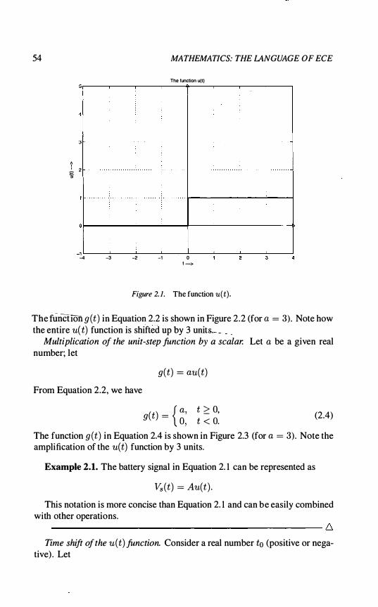
54 MATHEMATICS: THE LANGUAGE OF ECE
The function u(t) ,
� I 2 �
_1 L-__ � __ � ____ J-�� ____ � __ -L ____ L-__ � -4 -3 -2 -1 0
t ->
Figure 2. 1. The function u(t) .
The functiOn g(t) in Equation 2.2 is shown in Figure 2 .2 (for a = 3) . Note how the entire u( t) function is shifted up by 3 units. __ _ _
Multiplication of the unit-step function by a scalar. Let a be a given real number; let
From Equation 2.2, we have
g(t) = au(t)
g(t) = { �: t 2: 0, t < O. (2.4)
The function g(t) in Equation 2.4 is shown in Figure 2.3 (for a = 3) . Note the amplification of the u(t) function by 3 units.
Example 2.1. The battery signal in Equation 2. 1 can be represented as
Vs(t) = Au(t) .
This notation is more concise than Equation 2. 1 and can be easily combined with other operations. ------------------------------------------- 6
Time shift of the u(t) function. Consider a real number to (positive or negative) . Let

Signals in engineering
The fUnction 9(1) = u(t) + 3
g(t)
u(t)
-�4L-----_3L-----_�2-----_�t----��----L-----�----�----�
t -->
Figure 2.2. The function g(t ) = u(t) + a, a = 3.
The function g(t) = 3u(t)
g(t)
u(t)
_t L-____ L-____ � ____ J_ ____ � ____ _L ____ _L ____ � ____ � -4 -3 -2 -t
t -->
Figure 2.3. The function g(t) = au(t ) , a = 3.
4
55
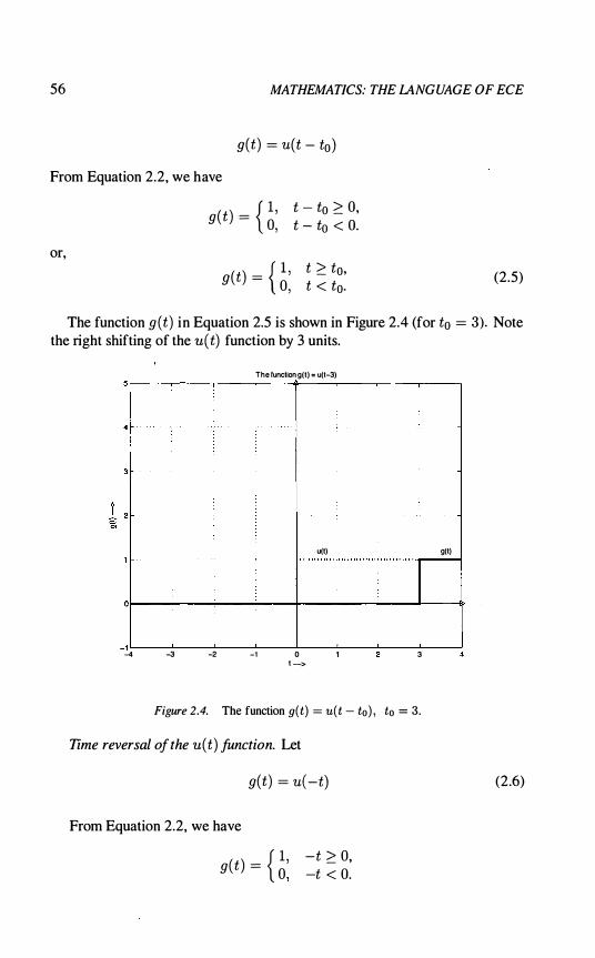
56 MATHEMATICS: THE LANGUAGE OF ECE
g(t) = u(t - to)
From Equation 2.2, we have
or,
g(t) = { 01 ,' t - to � O, t - to < O.
g(t) = { I , t � to, 0, t < to.
(2.5)
The function g(t) in Equation 2.5 is shown in Figure 2.4 (for to = 3). Note the right shifting of the u ( t) function by 3 units.
The funclion g(l) = u(I-3)
u(l) g(l)
_1 L-__ � __ -L ____ L-__ � __ -L __ �� __ � __ �. � � � � 0 3
t -->
Figure 2.4. The function g(t) = u(t - to) , to = 3.
Time reversal o/the u(t) function. Let
g(t) = u( -t)
From Equation 2.2, we have
g(t) = { 01 " -t � 0, -t < O.
(2 .6)

Signals in engineering
or,
g(t) = { 1 , t :::; 0, 0, t > O.
57
(2.7)
The function g(t) in Equation 2.7 is shown in Figure 2.5 . Note how g (t) is the mirror image of u( t) around the vertical axis.
The function g(l) = u( -I)
4
g(l) u(l) 1-------"----1 .. " .. " . . . . . . .. . . . . . . . . " " . . . . . . . . . . . . . . . . . . . . . . . .
- 1 '-_--'-_---..J'--_---'-_--' __ -L-_--'-__ ..I....-_--' -4 -3 -2 -1 o
t -->
Figure 2.5. The function g(t ) = u ( -t) .
Time scaling of the u( t) function. Consider a real number a > O. Let
g(t) = u(at) From Equation 2.2, we have
or, since a is positive,
g(t) = { �: at � 0, at < O.
g(t) = { 01 " t � 0, t < O. (2. 8)
The function g(t) in Equation 2.8 is, therefore, equal to u(t) . Scaling the time argument of the u( t) function by a positive factor has no effect on it. Intuitively, this should be expected, since shrinking or expanding either "branch" of the u(t) function should not change its shape.
Consider next a real number a < O. Let

58 MATHEMATICS: THE LANGUAGE OF ECE
g(t) = u(at)
From Equation 2.2, we have
or, since a is negative,
g(t) = { �: at 2: 0, at < O.
g(t) = { 01 " t :S 0,
t > O. (2.9)
The function g(t) in Equation 2.9 is, therefore, equal to u( -t) . Scaling the time argument of the u( t) function by a negative factor has the same effect as time reversal .
Point-wise addition and subtraction. Consider the point-wise addition of the u(t) function and some other functions we derived in this section. A number of other very common signals can be derived, as we will see in the following examples.
Example 2.2. (Unit step plus unit step reversed.) Let
f(t) = u(t) + u( -t)
f(t) i s the sum of the unit step function and its time-reversal (see Equation 2.6). Inspecting figures 2. 1 and 2.5, we can easily see that
f(t) = 1 ,
for all values of t except t = 0, for which f(O) = 2 .
Example 2.3. (Unit step minus unit step shifted.) Let
f(t) = u(t) - u(t - to ) (2. 1 0)
f (t) is the difference of the unit step function and its time-shifted version. Suppose that to is positive. Inspecting figures 2. 1 and 2.4, we can easily see that
f(t) = { I , O :S t � to, 0, otherwIse. (2. 1 1 )
For a more rigorous proof of the validity of Equation 2 . 1 1 , we can examine the value of the function f(t) in three regions:

Signals ill engineering 59
Region 1 , t < O. For all such t we have both u(t) = 0 and u(t - to) = O. Therefore, for all t < 0 we have f (t) = O.
Region 2, 0 � t < to . For all such t we have u(t) = 1 and u(t - to ) = O. Therefore, for 0 � t < to we have f(t) = 1 - 0 = l.
Region 3 , t 2 to. For all such t, we have both u(t) = 1 and u(t - to) = l . Therefore, for all t 2 to we have f(t) = 1 - 1 = 0 , proving the validity of Equation 2. 1 1 . --------------------------------------------- �
1.2 The unit pulse signal
The function f (t) in Equation 2. 1 1 represents a very common signal in ECE, called a pulse with unit amplitude and duration to time units or unit pulse, for short. A more common notation for the unit pulse is p(t ) . This signal is shown in Figure 2.6 (for to = 3).
1 .5
p(t) = u(t) - u(t - to) = {01 " 0 � t < to, otherwise.
The pulse function with unit amplitude and duration 3 time units
1 _ 0.5 '6:
-0.5
1 �--�--�----J---�----�--�----�--� -4 -3 -2 -1 0
t -->
Figure 2.6. The pulse with unit amplitude and duration to time units, to = 3.
(2. 1 2)

60 MATHEMATICS: THE LANGUAGE OF ECE
1 .3 The centered unit pulse signal
Another very common signal, closely related to the unit pulse in Equation 2 . 1 1 is the signal PT (t) , called the centered unit pulse of duration 7 and denoted by
-7/2 ::; t < 7/2, otherwise.
This signal is shown in Figure 2.7.
�
The centered unit pulse signal P't(t)
1.5
0.5
-0.5
-�L---��----_�2----_�1----LO ----L---�--�--� t -->
Figure 2. 7. The centered unit pulse signal PT (t) , with T = 1 .
1.4 The 8(t) function
(2. 1 3)
This function can be thought of as a limiting case of a unit pulse. Let
(2. 14)
be a pulse of duration 7, the amplitude of which is equal to 1/7. The integral of f T (t) (the area under the curve) is equal to 1 , regardless of the value of 7. Consider the limiting case of this signal , as 7 -> O. The integral is still equal to 1 , while the width of the pulse is O. We define the 8 (t) function as
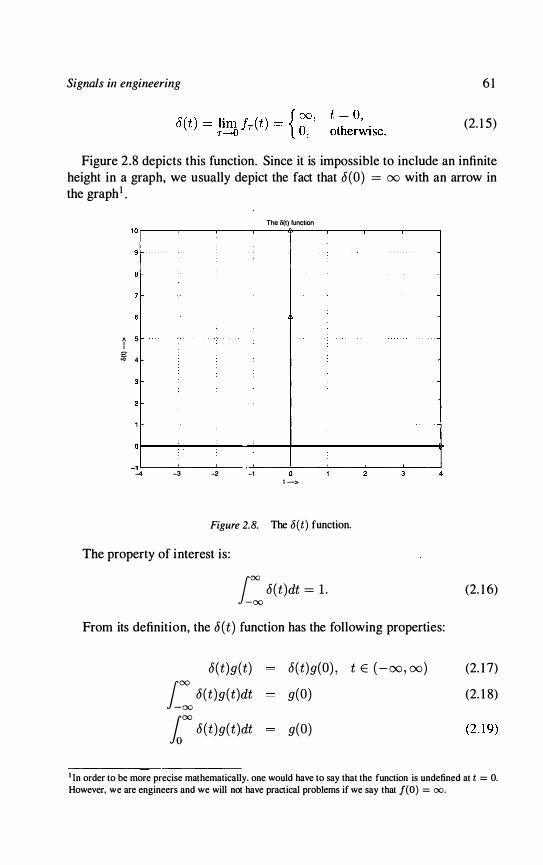
Signals ill engineering 6 1
(2. 1 5)
Figure 2.8 depicts this function. Since it is impossible to include an infinite height in a graph, we usually depict the fact that 8(0) = 00 with an arrow in the graph! .
The 6(1) function 1 0 ,----,----.----.----+----.----.----.----,
A 5 i � 4
_I � __ -L ____ � __ � ____ � __ � ____ � __ � ____ � -4 -3 -2 -I
. ->
Figure 2.8. The o(t) function.
The property of interest is:
L: 8(t)dt = 1 . From its definition, the 8 (t) function has the following properties:
8(t)g(t) L: 8(t)g(t)dt
100 8(t)g(t)dt
8(t)g(0) , t E (-OO, oo)
g(O)
g(O)
(2. 1 6)
(2. 1 7)
(2. 1 8)
(2. 1 9)
I In order to be more precise mathematically. one would have to say that the function is undefined at t = O. However, we are engineers and we will not have practical problems if we say that f(O) = 00 .
62 MATHEMATICS: THE LANGUAGE OF ECE
I: J(t - to )g(t)dt = g(to ) (2.20)
Example 2.4. Let's calculate the following integrals (we will see versions of some of them again as Laplace and Fourier transforms, in chapters 8 and 10) .
Al LX! J(t)e-5tdt
A2 = i: J(t - 5)e-6tdt
A3 LX! J(t)e-3t sin(27r1000t)dt
A4 i: [J(t - 1 ) + J(t + 1 ) ] e-2t cos(27r60t)dt
Applying Equation 2 . 1 9 with g(t) = e-5t , we have
Al = g(O) = e-5.O = 1 .
Applying Equation 2.20 with g(t) = e-6t and t o = 5, we have
A2 = g(5) = e-6.5 = e-30 ::::::: O .
Applying Equation 2. 1 9 with g(t) = e-3t sin(27r1000t ) , we have
A3 = g(O) = O.
Applying Equation 2.20 twice, with g(t) = e-2t cos(27r60t) and to = ±1, we have
A4 I: [J (t - 1 ) + J(t + 1 )] e-2t cos(27r60t)dt
= i: J(t - 1 ) e-2t cos(27r60t)dt + I: J(t + 1 )e-2t cos(27r60t)dt
g ( l ) + g( - 1 ) e-2. I cos(27r60 · 1 ) + e-2. (- 1 ) cos(27r60 · (- 1 ) ) e-2 cos(27r60) + e2 cos( -27r60) = e-2 + e2 ::::::: 7.52
-------------------------------------------,. 6

Signals in engineering 63
1.5 Clock generator signals
In digital ASICs (e.g . , CPUs, memory chips) a very fundamental signal is the "clock generator" signal. This is a periodic signal that looks like the one in Figure 2.9. This i s the basic signal that controls operations of the ASIC chips. For example, a CPU command may be given when the signal is "high"; the chip executes the command when the signal is "low" and the procedure repeats for the next command. A second example: a memory chip gets a read command when the signal is "high"; the chip makes the result of the read operation available when the signal is "low".
�u
The clock generator signal. Pelt)
1 .5
1 - ;-- r-- r-- r--
o. 5
o
-0. 5
1 -0.25 -0.2 -0.1 5 -0.1 -0.05 0 0.05 0.1 0.15 0.2 0.25
t ->
Figure 2. 9. The clock generator signal, Pc (t ) .
The clock generator signal , Pc(t) , in Figure 2.9, can be mathematically represented as a sum of time-shifted versions of the centered unit pulse signal , Pr (t ) , in Equation 2. 1 3 . In general, we can write
00
Pc(t) = L Pr (t - n2T - T/2) (2.2 1 ) n = - oo
Note that even though the summation in Equation 2.2 1 contains an infinite number of terms, one and only one of these terms can have a nonzero value for any given time t . For example, when t = 0, all terms Pr (t - n2T - T/2) are equal to 0, except for the n = 0 term, which is equal to 1 .
64 MATHEMATICS: THE lANGUAGE OF ECE
Example 2.5. Another representation of the clock generator signal , Pc{ t) , in Figure 2.9, is also possible, as a sum of time-shifted versions of the unit pulse signal, p{t) , in Equation 2. 1 2. Indeed, let to = 0.05 be the parameter of the unit pulse signal . Then, we can write
00
Pc{t) = L p{t - nO. I ) n=-oo
(2.22)
For any given value oft , again one and only one of the terms in the summation can have a nonzero value. ------------------------------------------- �
2. Sinusoidal signals
Many voltage and current sources used in electrical circuits produce a voltage or current that oscillates between a minimum and maximum value in a sinusoidal fashion. This time behavior is due, for example, to the rotation of a magnet inside an electric field. This signal behavior is modelled mathematically by the sinusoidal functions we have seen in Chapter I , Section 5 .
As we will witness in Chapter 9 , sinusoidal signals can be used to approximate other periodic signals. These approximations facilitate analysis of signals tremendously, as we will also see in the same chapter. For this reason, we review the properties of the sinusoidal functions here in detail .
2.1 Parameters of sinusoidal signals
Sinusoidal signals are represented mathematically using either a sine or cosine function. Recall the definition of the sine signal from Chapter I , Section 5 (see Figure 1 .20, page 29):
J {t) = A sin{wot + 0) = A sin{211"Jot + 0) , t E {-oo, 00) (2.23)
The cosine form is given as
J {t) = A cos{wot + 0) = A cos{211"Jot + 0) , t E (-oo, 00) (2.24)
Since
sin {x ) = cos {x - 11"/2) ,
it suffices to deal with one function only. (For most ECE applications, the cosine form is preferred.)
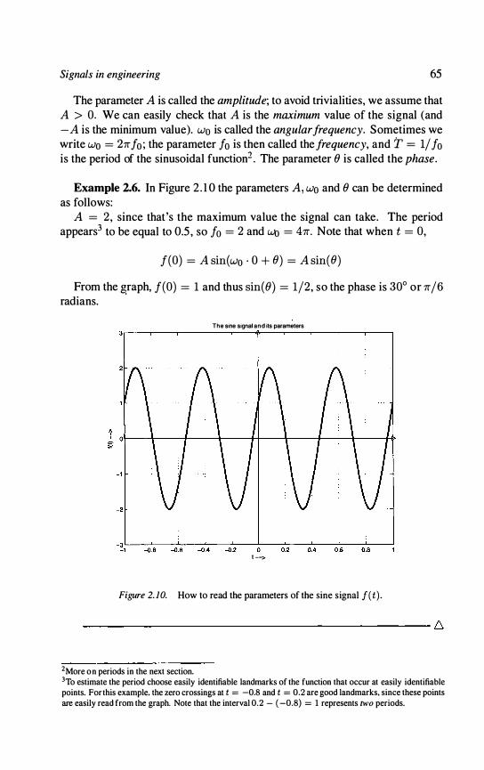
Signals in engineering 65
The parameter A is called the amplitude; to avoid trivialities, we assume that A > O. We can easily check that A is the maximum value of the signal (and -A is the minimum value). Wo is called the angular frequency. Sometimes we write Wo = 27r fo ; the parameter fo is then called the frequency, and T = 1/ fo is the period of the sinusoidal function2 • The parameter () is called the phase.
Example 2.6. In Figure 2 . 1 0 the parameters A, Wo and () can be determined as follows:
A = 2 , since that 's the maximum value the signal can take. The period appears3 to be equal to 0.5 , so fo = 2 and Wo = 47r. Note that when t = 0,
f(O) = A sin(wo ' 0 + ()) = A sin(())
From the &raph, f(O) = 1 and thus sin( ()) = 1/2, so the phase is 30° or 7r /6 radians.
The sine signal and its parameters
-� lL
--_��
.8---_�O.6---_�O
L.4 --���.2--
�O--
�O.�2 --�O
L.4 --�O�,6--
�O,8�
�
t -->
Figure 2. 10. How to read the parameters of the sine signal f(t ) .
2More on periods in the next section. 3To estimate the period choose easily identifiable landmarks of the function that occur at easily identifiable points. For this example. the zero crossings at t = -0.8 and t = 0.2 are good landmarks. since these points are easily read from the graph, Note that the interval 0.2 - ( -0.8) = 1 represents two periods.
66 MATHEMATICS: THE LANGUAGE OF ECE
2.2 Operations on sinusoidal signals
The following operations on sinusoidal signals are of special interest for two reasons:
They appear frequently in circuit applications.
2 They are extensively used in the mathematical analysis of other signals (see Chapter 9).
Addition/subtraction of sinusoidal signals, same frequency. From Equation 1 .30, page 30, in Section 1 .5 .3 , we can observe that adding or subtracting sinusoidal signals of the same frequency (taking linear combinations of such signals, to be more exact) does not affect the frequency of the signals, only their phase and magnitude, since it results in a sinusoidal signal of the same frequency.
Example 2.7. Let
h (t) = A sin(wot) , !z(t) = B cos(wot) .
where A = 3, B = 4 and Wo = 2 . Then, from Equation 1 .30 we can write:
g(t) h (t) + !z(t) A sin(wot) + B cos(wot) V A2 + B2 cos(wot - arctan(A/ B) ) V32 + 42 cos(wot - arctan(3/4) ) 5 cos(wot - 37° )
(2.25)
Figure 2. 1 1 depicts the signals h (t) and g(t) . It should be clear from the figure that the frequency of h (t) , g(t) is the same; from the t = 0 point, we can read that g(O) :::::: 4, and thus cos( 0) :::::: 4/5 which gives a phase of 37° .
---------------------------------------------- 6 This property will come in handy when we discuss the output of a linear
system (like an electrical circuit) when its input is a sinusoidal signal . Multiplication of two sinusoidal signals. From Equations 1 .3 1 , 1 .32 and
1 .33 in Chapter 1 , Section 5 .3 , we can observe that multiplying two sinusoidal signals results in the sum of two sinusoidal signals (of different frequencies) .
This property is essential in understanding modulation of signals, the fundamental property in radio and TV station transmission. It is also crucial in understanding how multiplication changes the period of the sinusoidal signals.

Signals in engineering
! :f;1\ L\ I\f �r\ ;1· · � · �v � V -5
.
- 10 -5 0 5 1 0
�l;;¥f�J -1 0 -5 0 5 1 0
� :r\jA r\j f-f\f (\ 1 -5 _ • V � vJJ _ V _ V_ -10 -5 0 5 1 0
t ->
Figure 2. 1 1. Addition of sinusoidal signals, same frequency.
Example 2.8. Figure 2 . 1 2 depicts the signals
h (t) sin(t) h (t) sin(2t) g(t) h (t) . h (t)
67
It should be clear from the figure that g(t) is periodic. The period of g(t) appears to be around 6. We will see how we can rigorously determine the period of such products (and sums) in Section 4. 1 .2 of this chapter. --------------------------------------------- 6
Time-shifting of a sinusoidal function. Let
We can write
f(t) A sin(wot + O) y(t) f(t + to) = A sin(wo(t + to) + 0)
y(t) = A sin(wot + woto + 0) = A sin(wot + ¢)
In other words, time-shifting of a sinusoidal signal simply changes its phase.

68 MATHEMATICS: THE LANGUAGE OF ECE
� :f· · •. . . · · ·6· ��hQ· •. /'\�' . . -1� . . ' .. . . _2 '--------'----"----...1....--------',----------L.----'
-10 -5 0 5 10
�. J� -10 -5 0 5 10
� J� -10 -5 0 5 10
1 ->
Figure 2. 12. Multiplication of two sinusoidal signals.
Time-scaling of a sinusoidal function. Let a =I 0 be a real number. Let
We can write
f(t) A sin(wot + 0) y(t) f(at)
y(t) = A sin(wo(at) + 0) = A sin( (awo ) t + 0)
In other words, time-scaling of a sinusoidal signal simply changes its frequency.
Example 2.9. Let
f(t) = 4 sin(t + 7f/6) y(t) = f(2t) = 4 sin(2t + 7f/6)
Figure 2. 1 3 depicts the two signals. It should be clear from the figure that the frequency of y (t) is twice that of f(t) , and the phase and magnitude remained unchanged. -------------------------------------------- 6

Signals in engineering
Figure 2. 13. Time scaling of the sine signal.
3. Exponential signals
69
Electrical circuits with capacitors and resistors produce voltage or current outputs that "decay" in time, starting from a "high" value initially and approaching 0 eventually. This time behavior is due, for example, to the phenomenon of capacitor discharging through a resistor in an RC circuit. This signal behavior is modelled mathematically by the exponential function we have seen in Chapter 1 , Section 4.
Let's recall the definition of the exponential function (see Figure 1 . 19 , page 27) :
f(t) = Aeat , t E (-OO, oo) (2.26)
where the parameter A is called the amplitude. The function
g(t) = Aeatu(t) , t E (-00, (0) (2.27)
with a < 0 can be used to describe the phenomenon of capacitor discharge we mentioned before. Figure 2. 14 depicts a typical example. The initial time is marked as t = O. The initial voltage is A. Note how multiplication by the u(t) function nullifies the values of the exponential function for al l negative times.

70 MATHEMATICS: THE LANGUAGE OF ECE
I(t) = Ae"u(t). A=1 .a=-1
1 .5
0.5
-D.5
_1 '---_-L.. __ --'-___ '-__ -L... __ --'-__ --' -1 2
t ->
Figure 2. 14. Decaying oscillations.
3.1 Cosine times exponential signals
Some electrical circuits with capacitors and resistors produce voltage or current outputs that both "decay" in time (starting from a "high" value initially and approaching some constant value eventually) and "oscillate" at the same time, as Figure 2. 1 5 depicts. We will discuss this time behavior in Chapter 7 , when we discuss differential equations and their application in circuits . This signal behavior is modelled mathematically by the product of the exponential function and a sinusoidal function we have seen in Chapter 1 , Section 4:
f(t) = Aeat cos(Wot)U(t) , t E (-00, 00) (2.28)
4. Periodic signals
A periodic function is a function that, loosely speaking, "repeats itself" over and over again. Periodic signals are quite common in the ECE world; the most common are the sinusoidal functions/signals that we have described previously. The ubiquitous power distribution lines carry electricity everywhere in the form of a sinusoidal signal with a frequency of 50/60 Hertz4 . Your PC's
4 Note: 60 Hertz is the standard in the American hemisphere; 50 Hertz is the standard in Europe.

Signals ill engineering
1 .5
-1���--�--�--�--�--�--�--�--�� o 0.5 1 .5 2.5 3.5 4 4.5
t -->
Figure 2. 15. Decaying oscillations.
7 1
CPU (and many digital ASIC chips) i s controlled by a clock generator signal with a frequency of a few hundred MHz.
Example 2.10. Consider the clock generator signal in Figure 2.9, page 63. If the time unit in the figure is microseconds, the period of the generator is 0. 1 /-tsec and thus the frequency is 1 /0. 1 = 1 0 MHz.
-------------------------------------------,- � In this section we will focus on the fundamental mathematical parameter of
such signals, namely their period, and see how we can determine this parameter.
4.1 The period of a signal
Intuitively, the period of a periodic signal is the time span of the signal segment that "repeats itself' . Looking at Figure 2.9, which depicts a clock generator signal , the period is 0. 1 (time units), because the signal segment in the time interval [0, 0 . 1 ] repeats itself over and over again.
Mathematically, a periodic function is defined as follows:
Definition: The function f(t) is periodic, if for some constant T > 0 f(t) = f(t + T) , Vt E (-00, 00) . (2.29)

72 MATHEMATICS: THE lANGUAGE OF ECE
Observe from Figure 2.9 that, for example, the signal segment in the time interval [-0.2 , 0] repeats itself over and over again; hence T = 0.2 is a constant that fits the property in Equation 2.29. Observe also that the segment in the time interval [-0.2 , 0 .2] repeats itself; so T = 0.4 also fits this property. However, no segment in a time interval smaller than [0, 0 . 1] repeats itself. Therefore, T = 0 . 1 is the smallest number that satisfies property 2.29.
Definition: The fundamental period of a periodic function f (t) is the smallest number T > 0 (if it exists) that satisfies property 2.29.
We usually drop the adjective fundamental and call T the period of the function. We call an integer multiple of T Q period (instead of the period).
4.1.1 How to find the period of a function Given a graph of the function (or, in real life, an oscilloscope trace) , we can
determine its period by inspection. (The graph, however, would have to be infinitely accurate to yield the true value of the period.)
Example 2.11. Consider the clock generator signal depicted in Figure 2.9. The (fundamental) period of this signal is 0. 1 time units. The period of the signal f (t) in Figure 1 .20, page 29, appears to be around 6.2 (or 27r) time units. -------------------------------------------- 6
Alternatively, given a mathematical formula for the function, we can determine whether the function is periodic by checking whether Equation 2.29 applies. In order to show that a real number T is the period, we must show that no positive number smaller than T satisfies Equation 2.29.
*Example 2.12. Consider the cosine signal s(t) defined in Equation 2.30 below. Show that the signal is periodic with period T = 1/ F.
s (t) = cos(27rFt)
Let T = 1/ F. From Equation 2.30 we have
s(t + T) = s(t + 1/F) = cos(27rF(t + l /F) ) cos(27rFt + 27r) cos(27rFt) = s(t)
verifying that T = 1/ F is Q period.
(2.30)
(2.3 1 )
Signals in engineering 73
Suppose next that another number, 0 < T' < T is also a period. Let T' = 1/ F'. We must have, then, by assumption:
F' > F. (2.32)
Since T' i s also a period, we must have 8( t + T') = 8( t) , for all values of t . Let t = O. We must have
8(0) 8(0 + T' ) = 8(0 + 1/ F') = cos(271" F(O + 1 / F') ) cos(271" F / F')
However, 8(0) = cos(O) = 1 . Therefore, we must have cos (271" F / F') = 1 . This equation will be true only when
271"F/ F' = 0, 271", 471", 671", 871", . . .
or when
F/F' = 0, 1 , 2 , 3, 4 , . . .
The case F / F' = 0 is impossible; in all other cases, we have that F 2: F', a contradiction of the assumption in Equation 2.32. --------------------------------------------- 6
Example 2.13. Consider the signal 8(t) defined in Equation 2.33. Show that the signal is periodic and determine three periods.
8(t ) = 10 + 50 cos(271"1000t - 7I"/3) +20 sin(271"1750t + 71"/4) + 2 sin(271"1500t + 71"/4) (2.33)
A period of the signal 8( t) is
T = 1 .
Indeed, from Equation 2.33 we have
8(t + 1 ) = 10 + 50 cos(271"1000(t + 1 ) - 71"/3) +20 sin(271"1750(t + 1 ) + 71"/4) +2 sin(271"1500(t + 1) + 71"/4) 10 + 50 cos(271"1000t + 271"1000 - 71"/3)

74 MATHEMATICS: THE LANGUAGE OF ECE
+20 sin(27f1750t + 27f1750 + 7f /4) +2 sin(27f1500t + 27f1500 + 7f/4) 10 + 50 cos(27f1000t - 7f /3) + 20 sin(27f1750t + 7f /4) +2-sin(27f1500t + 7f/4) (2.34)
= s( t) (2.35)
verifying that T = 1 is a period. In deriving Equation 2 .34, we used the fact that, for any real number x and integer k, we can write:
sin(x + 27fk) = sin(x) , cos(x + 27fk) = cos(x)
Since any integer multiple of a period is also a period, T = 2 and T = 3 are also periods of s(t) . (Note that finding the fundamental period of s (t) requires more effort.) -------------------------------------------- 6
4.1.2 Operations on periodic signals Consider two periodic signals Sl (t) and S2 (t) , with periods T1 and T2 re
spectively. These signals can get added, subtracted, multiplied. time-shifted. time-reversed and time-scaled. Is the resultant signal also periodic? If yes, what is its period? ·
We state a few results without proof.
THEOREM 2 . 1 Let Sl (t) be a periodic signal with period T1 . Let Ssh (t), ssc ( t) , srev ( t) , samp, Sbias be the time-shifted, time-scaled, time-reversed, "amplified" and "biased" versions of Sl (t) respectively, defined by
Ssh ( t) Sl (t - tO) ssc ( t) sl (at) , a of O
srev (t) Sl (-t) Samp CS1 (t) , c of O Sbias sl (t) + d, d of O
Then
• Ssh(t) is periodic with the same period T1 .
• Srev (t) is periodic with the same period T1 .
• ssc(t) is periodic with period Tsc = TI/ la l .
• samp( t ) is periodic with the same period T1 .
Signals in engineering 75
• Sbias (t) is periodic with the same period T1 .
THEOREM 2 . 2 Let Sl (t) be a periodic signal with period T1 . Let S2 (t) be a periodic signal with period T2• Let
Slin (t) Smult (t)
Cl Sl (t) + C2S2 (t) S l (t)S2 (t)
Suppose that the ratio TI/T2 is a rational number. Then
• Slin (t) is periodic.
• Smult (t) is periodic.
We will make use of these two theorems in Chapter 9. We ask you to prove some of these statements in the problem section.
Suppose that Tl = T2. The period of (each 00 the signals Slin (t) , smu!t (t) is not necessarily the same as T1 , as the following simple examples demonstrate.
Example 2.14. Let C2 = Cl i= O. Let Sl (t) = S2 (t) = sin(t ) , with period Tl = T2 = 27r. Then
Slin (t) = Cl Sl (t) + C2S2 (t) = 2Cl S l (t) = 2Cl sin(t) = 2Cl sin (27r . 2� t)
Intuitively, T = Tl = 27r should be Q period. Following the procedure of Example 2 . 1 2, we can formally check that 27r is the period T of the signal Slin (t) . --------------------------------------------- 6
*Example 2.15. Let C2 = -Cl . Let Sl (t) = S2 (t) = sin(t) , with period Tl = T2 = 27r. Then
What is the period T of the signal Slin (t) (or of any constant-valued signal for that matter)? Intuitively, any positive real number T', no matter how small , would be Q period, since
0 = Slin (t) = Slin (t + T')
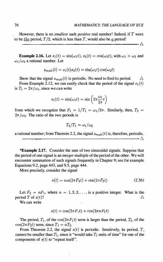
76 MATHEMATICS: THE LANGUAGE OF ECE
However, there is no smallest such positive real number! Indeed, if T were to be the period, T 12, which is less than T, would also be Q. period ! ------------------------------------------- 6
Example 2.16. Let Sl (t) = sin(wl t ) , S2 (t) = COS(W2t) , with WI > W2 and WI I W2 a rational number. Let
Show that the signal Smult (t) is periodic. No need to find its period. 6 From Example 2. 1 2, we can easily check that the period of the signal Sl (t)
is Tl = 27f IwI , since we can write
Sl (t) = sin(wl t) = sin (27f;� t) from which we recognize that Fl = 11Tl = wd27f. Similarly, then, T2 =
27f I W2 . The ratio of the two periods is
a rational number; from Theorem 2.2, the signal Smult (t) is, therefore, periodic. -------------------------------------------- 6
*Example 2.17. Consider the sum of two sinusoidal signals. Suppose that the period of one signal is an integer multiple of the period of the other. We will encounter summation of such signals frequently in Chapter 9; see for example Equations 9.2, page 443, and 9.5 , page 444.
More precisely, consider the signal
(2.36)
Let F2 = nFl , where n = 1 , 2 , 3 , . . . , is a positive integer. What is the period T of s(t)? 6
We can write
The period, T1 , of the cos( 27f Fl t) term is larger than the period, T2 , of the cos(27f F2t) term, since Tl = nT2 .
From Theorem 2.2, the signal s(t) is periodic. Intuitively, its period, T, cannot be smaller than T1 , since it "would take Tl units of time" for one of the components of s( t) to "repeat itself".

Signals in engineering
Let's guess, then, that T = TI is a period of 8(t ) . We have
8(t + T) 8(t + Td cos(27l" FI (t + 1/ Ft } ) + cos(27l"nFI (t + 1 / FI ) ) cos(27l"Fl t + 27l") + cos(27l"nFl t + 2n7l") cos(27l"Fl t) + cos(27l"nFlt) · 8(t)
verifying that indeed, TI i s a period of 8(t) .
77
As in Example 2. 1 2, suppose next that another number, 0 < T' < TI is also a period. Let T' = 1 / F' . We must have, then, by assumption:
F' > Fl . (2.37)
We will show that 8 (0 + T') =I- 8(0) , contradicting the definition of periodicity. We have
8(0) 8(0 + T')
cos(27l" FI . 0) + cos(27l"nFI . 0) = 2 cos(27l" FI . T' ) + cos(27l"nFI . T' ) cos(27l" Fd F') + cos(27l"nFd F') (2.38)
The only way for the right-hand side of Equation 2.38 to equal 2 is when both
cos(27l" Fd F') = 1 , and cos(27l"nFd F') = l .
Since FdF' < 1 (and F' < 00), we have cos(27l"FdF') < I , verifying that 8(0 + T') =I- 8(0) . --------------------------------------------- 6
4.2 Approximations of periodic signals
A periodic signal can be approximated (like almost any other function) via polynomial signals . For example, we have seen the Taylor series expansion of the sine function, in Chapter I , Section 5 .2, which we repeat here:
• 00
k (t)2k+1 sm(t) = Z )-I )
(2k ) 1 k=O + 1 .
A polynomial approximation is obtained by using only a finite number of terms in the summation. Polynomial functions are not periodic . Another approximation of a periodic signal , via sinusoidal signals, is also possible. This

78 MATHEMATICS: THE LANGUAGE OF ECE
approximation is the essence of the Fourier series representation of a periodic signal in Chapter 9, one of the main topics of this book; see, for example, in Figure 9. 1 , page 443, how well the clock generator signal can be approximated with a few sinusoidal functions.
s. Time shifting and scaling of signals
5.1 Time scaling in real life
Time scaling is very common in practice. Electrical signals, especially periodic ones, are frequently time scaled, when displayed in oscilloscopes. For example, a 1 0-inch screen can display only so many samples of a signal . When more samples need to be depicted, the signal must be "squeezed"; this is equivalent to time-scaling the signal by a factor a > 1 . When fewer samples need to be depicted, the signal is "stretched"; this is equivalent to time-scaling the signal by a factor a < 1 .
Another instance of time scaling is the change of a frequency oscillator device in a printed circuit board (PCB) . For example, the (Ethernet) network card of your PC has, in all likelihood, a 100 Mbps (Megabits per second) adapter. In this PCB, a frequency oscillator producing a clock generator signal of x MHz is used. If the adapter were to be upgraded to 1 000 Mbps, the Gigabit Ethernet technology, the clock generator signal is probably changed (time scaled) to lOx MHz. A challenge in the design of PCBs is to make sure that the electrical circuits are designed such that they work with the time scaled signals as well .
Many analog sensors use time scaling to indicate the change in a physical quantity. For example, a common vacuum sensor in a car changes frequency as a function of pressure.
5.2 Time shifting in real life
From Chapter 1 , Section 1 .3 .5 you should have gained some experience about shifting a signal s ( t) by to time units to the left (s ( t + to ) or to the right (s(t - to) . In practice, what causes shifting of an electrical signal? One very common cause is the finite speed of light. For the purposes of this discussion, we may assume that the speed oflight is 300,000,000 meters/sec. Let's consider two �cenarios.
5.2.1 Shifted signals with small to values. Your PC has a microprocessor (CPU) and multiple memory chips, placed
on a board. A network router has a similar arrangement of CPU and memory chips. The memory chips are not always the same distance away from the CPU. When the CPU issues a command to read data from the memory chips, the electric current that excites memory chip A and chip B will have to travel

Signals in engineering 79
different distances. Therefore, the results of the read command will come back to the CPU at different times.
Example 2.18. Consider a CPU and two memory chips, placed dA and dB meters away from the CPU, where dA > dB . (Typical values for dA and dB are a few centimeters. ) The read command from the CPU is a pulse of the form
s(t) = u(t) - u(t - T) .
A typical value for fast CPUs is T = 10 nanoseconds (ns). Therefore, the read command is a "pulse" with a IO ns duration. If we put an oscilloscope probe at the CPU pins, and record the read command, we will observe the signal s(t) . If we put a second probe at memory chip A, and record the read command, what signal will we observe? If we put a second probe at memory chip B, and record the read command, what signal will we observe?
A moment's reflection should convince you that the signals we will observe at the two memory chips will be time-shifted versions of s(t ) . The mathematical expressions for the two signals in question, as a function of s(t ) , dA and dB i s left as an exercise. --------------------------------------------- 6
Example 2.19. Consider how cell phones work: the signal s(t) from the antenna of a cell phone is transmitted to the antenna of a base station. Suppose that the two antennas are dA meters apart. The antenna of the base station receives the signal s (t) and at least one more copy of it, due to reflections of the signal over buildings, trees, etc . Consider, for simplicity, only one such reflection, denoted by Sr (t) . Because Sr (t) travels a larger distance, it will be a delayed (and quite likely an attenuated) version of s(t ) , i .e . ,
sr (t) = s(t - to)
for some to > 0 that depends on the length of the reflection path. An obvious question of practical interest is whether the reflected signal will
"distort" the original one. We present some specific exercises in Chapter 3 , after we discuss how to generate accurate signal plots. --------------------------------------------- 6
5.2.2 Shifted signals with humongous to values. When communicating with (deep) space crafts, electromagnetic signals sent
from the earth stations to control the crafts have to travel extremely long distances. This causes a time shift; a command issued from the earth control station at time t will be received by the craft at some later time. The larger the distance of the craft from the earth, the larger this delay will be.
80 MATHEMATICS: THE LANGUAGE OF ECE
When a spacecraft enters the gravitational field of a planet, special rockets have to be fired, to adjust the craft's speed and make sure that a proper orbit is entered. The firing must take place when the craft is at a given distance from the planet. The margin for error is not large, due to limitations on fuel quantity.
Example 2.20. Consider a spacecraft that is supposed to explore Pluto. The spacecraft rockets must be fired when the craft is, say, about 20,000 miles away from Pluto's surface, in order to put the craft in a circular orbit around it. The distance between Earth 's and Pluto's surfaces is d millions of miles (perhaps you can find the actual value of d from a website or something) . The craft is launched on January 1 , 2000, 00:00 hours, which we can call time t = O. The $ IM question is : at what time should the rocket firing command be sent to the craft?
Because the speed of light is finite, the radio signal to the craft will be a delayed version of the signal sent to it. If the command must be received at the craft at time t, it must be sent from the control station at time t - to , where to is definitely not in the seconds range. -------------------------------------------- 6
5.3 Time shifting and scaling of pulse-shaped signals
In this section let's work out an example of the effects of time shifting and scaling on a pulse-shaped signal. A thorough command of these effects will make understanding the respective theorems in Fourier and Laplace transforms much easier.
Example 2.21. Simple time shifts. Consider p(t), the unit pulse signal in Equation 2. 1 2, page 59. Let to = 10. The duration of this pulse is 1 0 units. The pulse has a nonzero value only in the interval [0, 10] .
Consider the signal hI (t) , with a value of 1 in the interval [200, 210) (and a value of 0 everywhere else) . Mathematically, we can write:
h (t) = { I , 200 :::; � < 210,
1 0, otherwIse. (2.39)
In a more compact notation, we can use the signal p(t) and time shifting to write hI (t) as:
hI (t) = p(t - 200) .
The signal h2 (t) , with a value of 1 in the interval [-20, - 10) (and a value of 0 everywhere else) can be written as
h (t) = { I , -20 :::; . t < -10,
2 0, otherwIse,
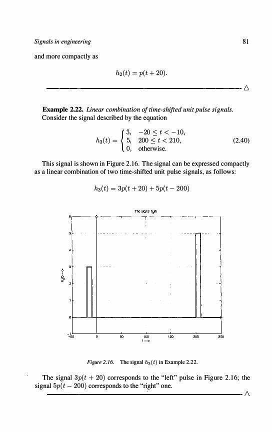
Signals in engineering 8 1
and more compactly as
h2 (t) = pet + 20) .
---------------------------------------------- 6
Example 2.22. Linear combination of time-shifted unit pulse signals. Consider the signal described by the equation { 3. -20 < t < - 10,
h3 (t) = 5, 200 :S t < 210 , 0, otherwise.
(2.40)
This signal is shown in Figure 2. 1 6. The signal can be expressed compactly as a linear combination of two time-shifted unit pulse signals, as follows:
h3 (t) = 3p(t + 20) + 5p(t - 200)
2
o���+_------------------------�----�
-k�----7-----�50�--�1�OO----�1��--�2�OO-----7.250 t -->
Figure 2.16. The signal h3 (t) in Example 2 .22.
The signal 3p( t + 20) corresponds to the "left" pulse in Figure 2. 1 6; the signal 5p(t - 200) corresponds to the "right" one. --------------------------------------------- 6

82 MATHEMATICS: THE LANGUAGE OF ECE
Example 2.23. Simple time scaling. Considerp( t ) , the unit pulse in Equation 2. 1 2, page 59. Let to = 10.
Consider the signal h4 (t) , defined by
h (t) = { 1 , 0 ::; t .::= 300,
4 0, otherwIse. (2.4 1 )
This signal i s a "stretched" version of p( t) (recall the discussions i n Section 1 . 1 .3 .7 . ) We can express h4 (t) via a time-scaled version of pet) as follows:
h4 (t) = p(t/30) (2 .42)
(Recall from the discussions and examples in Section 1 . 1 .3.7 that the scaling factor should be less than 1 .) We can check that Equation 2.42 is correct as follows: for any value of t in the interval [0, 300) , the number t/30 will belong to the interval [0, 10) . Therefore, for all such t , from Equation 2 .4 1 , we have that h4 (t) = 1 ; on the other hand, from Equation 2. 1 2 we have that p{t/30) = 1 = h4 {t) . So, equation 2.42 holds true for t in the interval [0, 300) .
Consider now any value of t < 0; then t/30 is also negative. We have both h4 {t) = 0 and p{t/30) = 0, so h4 {t) = p{t/30) for such values of t as well .
Consider, finally, values of t > 300; then t/30 > 10. For any such value of t, we can easily see that h4 {t) = 0 and p{t/30) = 0, so h4 {t) = p { t/30) for such values of t as well .
------------------------------------------- 6
Example 2.24. Simple time scaling. Consider p{ t) , the unit pulse in Equation 2. 1 2, page 59. Let to = 10.
Consider the signal h5 ( t) , defined by
h (t) = { I , 0 ::; t .::= 10/3, 5
0, otherwIse. (2.43)
This signal is a "shrunk" version of p et) . We can express h5 {t) via a timescaled version of p{ t) as follows:
h5 {t) = p{3t) .
The proof is entirely similar to the one in the previous example. -------------------------------------------,· 6

Signals ill engineering 83
*Example 2.25. Combined time shifting and scaling. s Consider p(t) , the unit pulse in Equation 2. 1 2, page 59. Let to = 10.
Consider the signal h6 (t) , with a value of 5 in the interval [ 100, 300) and o everywhere else; this signal cannot be written as a simple shifted version of p( t ) , since its ouration is 200, not 1 0 time units. It cannot be written as a simple scaled version either, since the scaled version will be nonzero outside the interval [100, 300] . A combination of time shifting and scaling is called for here.
We have two options to try out: Option 1 : First scale then shift. Observe that the length of the interval over
which h6 (t) is nonzero is 300 - 100 = 200 time units. We can scale p(t) by a factor of a = 10/200 = 1/20 to match this length. Let 's write
y(t) = p(at) = p(t/20)
Note that y(t) has nonzero values in the interval [0, 200) . Now, shifting y(t) by an amount of tl = 100 units to the right would be the appropriate one, so we can write
h6 (t) = y(t - tl ) = p(a(t - tl ) ) = p((t - 100)/20) = p(t/20 - 5)
Note that we can rewrite this equality as
(2.44)
Option 2: First shift then scale. Suppose we time-shift first; what is the proper value for the shift?
Let's say we try t2 = 100 units to the right. Let
g(t) = p(t - t2) = p(t - 100)
denote the time shifted version of p( t) . The scaling factor should be a = 1/20 as in option 1 , since we must still
cover an interval of length 200. So, we must have
h7 (t) = g(at) = p(at - t2 ) = p(t/20 - 100)
But this does not match what we obtained in option I , i .e . , h7 (t) -=I- h6 (t) . Let's check this by considering the value at t = 140. Let t = 140 in this last expression. We have
5Notice that there are no figures in this example. This is done on purpose. It is imperative that you are able to follow the steps in this example " in your head" ; if you obtain this skill. you have nothing to fear in the three transform chapters.

84 MATHEMATICS: THE LANGUAGE OF ECE
h7 ( 140) = p(140/20 - 100) = p( -93) = 0
so we have done something wrong! A moment's reflection should convince you that the problem was with the selection of t2 , not a.
Observe that we can interpret the combination of "first shift then scale" operations as what the term p( at - atl ) Equation 2.44 describes. Then, according to this equation, the proper shift amount is t2 = atl = 100/20 = 5!
Try it out and check that it works. -------------------------------------------- 6
Example 2.26. Consider the signal s(t) defined by { I , 1 :S t < 3, s(t) = -1 , -3 :S t < -1 ,
0 , otherwise.
(This signal is shown in Figure 904, page 454.) We will express this signal as a linear combination of time-shifted versions of the centered unit pulse signal PT (t} in Equation 2. 1 3 , page 60.
Since each one of the pulses in Figure 9.4 has a width of 2 units, let T = 2. Then we can write
s(t) = P2 (t - 2) - P2 (t + 2)
The time-shifted pulse P2 (t - 2) accounts for the "right" pulse in Figure 904, while the time-shifted pulse P2 (t + 2) accounts for the "left" one. ----------------------------------------- 6
Example 2.27. Consider the signal v(t) in Figure 8.3 , page 428. We can express it as a linear combination of time-shifted versions of the centered unit pulse signal PT (t) in Equation 2. 1 3 , as follows:
v(t) = PI (t - 0 .5) + PI (t - 3 .5) .
------------------------------------------- 6
Example 2.28. Consider the signal v(t) in Figure 804, page 429. We can express it as a linear combination of time-shifted versions of the centered unit pulse signal PT (t) in Equation 2. 1 3 , as follows:
v(t) = PI (t - 0.5) - PI (t - 1 . 5 ) .
Signals in engineering 85
We can also express v( t) as a linear combination of time-shifted versions of the unit pulse in Equation 2. 1 2, with to = 1 . Indeed, we can write
v(t) = p(t) - p(t - 1 ) .
6. Summary of main points
• The unit-step function u( t) and its properties
time shifting time reversal multiplication by a scalar obtaining the various pulse signals from the u( t) function obtaining the clock generator signal from the u( t) function
• The sinusoidal function and its properties
time shifting simply changes the phase parameter Addition/subtraction of two sine functions of the same frequency produces a sine function of the same frequency (and different amplitude and phase) Addition/subtraction of two sine functions of different frequencies does not produce a sine function Multiplication of two sine functions produces a sum of two sine functions.
• The period of a function and how operations on a function change its period.
• Time shifting and time scaling operations on signals, especially pulses.
Skillset to be developed
• Develop expertise in algebraic operations (linear combinations, multiplication) of sinusoidal signals.
• Perform time-shifting, time-scaling operations on simple signals, like the unit pulse and sinusoidal signals .
• Determine the period of a signal, given a mathematical expression for the signal.
• Determine the period of a sum of sinusoidal signals.
• Determine analytic expressions for a "complicated" signal, using linear combinations of time-shifted, time-scaled, simpler signals .

86 MATHEMATICS: THE LANGUAGE OF ECE
Problems
The u ( t) function and its properties and transformations
2.1. Consider the u( t) function.
1 How many different values can u(t) have?
2 What is the function value for t = 1, i .e . , what is the value u( I ) ?
3 What i s the value u(lOOO)?
4 What is the value u( -I ) ?
5 What i s the value u ( - 1000)?
6 What is the value u(O) ?
7 For what value of t, if any, is u( t) = 1000?
8 For what value of t, if any, is u( t) = -I ?
2.2. Transformations of the u(t) function. Define new functions as follows:
Answer the following:
g(t) u( -t) f (t) -u(t) h(t) -u( -t) m(t) u(t) + u(-t) n(t) u(t) - u( -t) p(t) u(t) . u(t) q(t) u(t) . u( -t)
1 What are the values g( I ) , f( I ) , h( I ) ?
2 What are the values g( lOOO) , f(lOOO ) , h( lOOO) ?
3 What are the values g( -1 ) , f( -1 ) , h( - I ) ?
4 What are the values g( - 1000) , f( - 1000) , h ( - 1000)?
5 What are the values g(O ) , f(O) , h(O )?
6 What are the values m(I) , n (I ) ?

Signals in engineering
7 What are the values m(1000) , n( 1000)?
8 What are the values m( -1 ) , n( - I ) ?
9 What are the values m( - 1000) , n ( - 1000)?
1 0 What are the values m(O) , n(O)?
1 1 What are the values p(l) , q ( l ) ?
1 2 What are the values p( 1000) , q( 1000)?
13 What are the values p( - 1 ) , q( -I ) ?
1 4 What are the values p( - 1000) , q ( - 1000)?
1 5 What are the values p(O) , q(O)?
87
*2.3. Based on your practice with the previous problem, prove theoretically that
m(t) 1 , t # 0, p(t) u(t) , q(t) O, t # O.
2.4. Transformations of the u( t) function. Define new functions as follows:
Answer the following:
r(t) 5u(t) 8(t) -5u(t) v(t) u(3t)
1 What are the values r ( l ) , 8 ( 1 ) , v ( l ) ?
2 What are the values r ( 1000) , 8(1000) , v ( 1000)?
3 What are the values r( - 1 ) , 8( -1 ) , v ( - I) ?
4 What are the values r ( -1000) , 8( - 1000) , v( - 1000) ?
5 What are the values r(O) , 8(0) , v(O) ?
88 MATHEMATICS: THE LANGUAGE OF ECE
2.5. Based on your practice with the prev ious problem, prove theoretically that
v(t ) = u(t) (2 .45)
2.6. Transformations of the u(t) function. Define new functions as fol lows:
Answer the fol lowing:
w (t ) z ( t )
What are the values w(l ) , z ( l ) ?
u(t - 1 ) u(t + 1 )
2 What are the values w(lOOO) , z ( lOOO)?
3 What are the values w( - 1 ) , z( - 1 ) ?
4 What are the values w( - 1000) , z ( - 10 00)?
5 What are the values w(O) , z (O )?
(2.46)
(2.47)
2.7. Consider the functions defined in Equations 2.46 and 2.47. Define new functions as fol lows:
a(t) u(t + 1 ) - u (t - 1 ) b(t) u(t ) - u(t - 1)
Answer the fol lowing:
I What are the values a(-2) , a( - 1 . 5) , a (- l ) , a(-0 .5) , a(O), a(0 .5 ) , a ( l ) , a ( 1 .5 ) , a(2)?
2 What are the values b( -2) , b( - 1 . 5) , b ( - 1 ) , b( -0.5) , b(O) , b (0 .5) , b( l ) , b ( 1 .5 ) , b(2)?
2.8. Sketch the fol lowing functions [or t E [- 10, 10] by han(L. From the sketch determine:
• The maximum value of the function in the interval [- 10, 10] ; the value(s) of t for which the maximum occurs.

Signals in engineering 89
• The minimum value of the function in the i nterval [- 10, 10] ; the value(s) of t for which the minimum occurs_
• The zeroe s) , i f any, of the function in the interval [- 10, 10] _
S , ( t ) 'U(t) S2(t) 'U (t) + 3 S3(t) 5'U( t )
S,I ( t ) 'U(t - 1)
S5 ( t ) 'U (t + 1 )
S6 ( t ) -'U (t - 1 ) Si(t) 'U(t) - 'U(t - 1 )
2.9. You can use the sketches in the previous problem to visua l ize the answers to the fol l owing questions, but you need to prove them mathematical ly_
I Is S3 ( t ) 2': S l ( t ) for all t E [- 10_ 1O] ?
2 I s S5(t ) 2': S4 ( t ) for all t E [-10 , lOP
2.10. Using the unit step function sketch the fol lowing functions: (a) s , ( t ) = 'U( t - 2 ) (b) S2(t ) = 'U( t ) - 'U(t - 2) (c) S3 ( t ) = t ['U( t + 1 ) - 'U (t - 1 )] (d ) S_I ( t ) = 'U( t + 2 ) + 2'U ( t ) - 'U(t - 1 ) - 3'U(t - 3) + 'U( t - 4) (e) S5 ( t ) = s3 (2t - 4) (f) S6 (t ) = s4 ( -t/2)
2.1 1 . Are any of the fol lowing statements cOiTect? In other words, in which of the fol lowing in tegrals can we omit the 'U( t ) term? Explain why_
r IO Jo sin(s)'U (s)ds
j- lO sin( s )'U ( S )ds - 10 1-5 sin(s)'U (s)ds - 10 J sin(s) 'U(s)ds
110 sin(s )ds ?
j-lO sin(s)ds ? -10 j--5 sin(s)ds ? -10 J sin(s)cls ?

90 MATHEMATICS: THE LANGUAGE OF ECE
2.12. In this problem, k is a positive integer and a is a real number. To avoid trivial i ties, assume that a =1= O. Find the fol lowing derivatives:
d'U( t) dt h ( t )
h(t) d[v,( t ) - 'U( t - 1 ) ]
dt
h(t ) d['U (t ) - 'U( t - 1 )] t2
dt
The i5(t ) function and its properties
2.13. Calculate the fol lowing integrals
Al foOO i5(t )'U ( t )dt
A2 1: i5( t)'U(t )dt
A3 fooo i5 (t)e-4t sin(2n60t)dt
AI l: [i5(t - 5) + i5(t + l ) ] e- lO tdt
2.14. Calculate the fol lowing integrals
Al fo i5 ( t ) [e- lOt + sin(2n106t) ]dt
A2 1: i5( t - 5)e-6t'U (t)dt
A3 fooo i5 (t)e-3t ['U ( t ) - 'U( t + 2) ] sin(2nlOOOt)dt
2.15. Sketch the fol lowing signals
V I ( t ) i5 (t ) [e- I. + cos(2n106t)] V2 ( t ) i5(t - 5) + i5(t + 5) V3 ( t ) i5 ( t )e-3t ['U ( t ) - 'U ( t + 2) ] sin(2nlOOOt)
Signals in engineering
2.16. Sketch the following signals
Sinusoidal signals
Vl (t) O(t ) . O(t - 5) 5
V2 (t ) L O(t - k5)
00 V3 (t ) L O(t - k)
k=O
9 1
2.17. Consider the graph of the signal s(t) shown in Figure 2 . 1 7 . The graph is accurate. Which of the fol lowing statements could apply?
s(t) = sin(t)
2 s(t) = sin(t + 27f)
3 s(t) = cos(t - 7f/2)
4 none of the above
2.18. Let s(t) = sin(27ft ) . The period of thi s signal is T = l. Let y(t) = I s (t ) l ; y(t ) is cal led the rectified sinusoidal signal . It appears frequently in power conversion systems. Find the period of y( t ) .
2.19. Does the period o f a sinusoidal function depend on its phase? i ts ampli tude? Prove your answer mathematically.
Periodic functions
2.20. Consider the signal shown in Figure 2. 1 8. Determine i ts period by i nspection.
2.21 . Consider the signal shown in Figure 2 . 1 9. Determine its period by i nspection.
2.22. Consider the signal shown in Figure 2.20. Determine its period by inspection.

92 MATHEMATICS: THE LANGUAGE OF ECE
The signal s(l)
0.8
0.6
0.4
0.2
� Or-+---��---r----+---�-----r----+---��---r-i -0.2
-0.4
-1
1 .5
'" 0.5 ""
0
-0.5
-1 -2.5 -2
o time t -->
Figure 2. 1 7. Plot for an unknown signal.
A periodic pulse signal
-1 .5 -1 -0.5 0.5
Figure 2. 18. A periodic pulse signal.
10
1 .5 2.5

Signals in engineering
A periodic ramp signal
1 .5
-1 .5
_2 L-__ � ____ -L ____ � ____ � __ �L-__ -L ____ � ____ � ____ L-__ -J -5 -4
2.5
1 .5
� 0.5
go 0
-0.5
1
-1 .5
-2
-2.5 -4 -3
-3 -2 -1
Figure 2. 19. A periodic ramp signal.
�
A periodic signal
� � V �
-2 -1 o
Figure 2.20. A periodic signal.
2
V V
93

94 MATHEMATICS: THE LANGUAGE OF ECE
2.23. Consider the sine signal s(t ) defined in Equation 2.48 below, with nonzero parameters A, F, B. Show that the signal is periodic with period T = l /F.
s(t) = A sin(21TFt + B) (2.48)
r . • Consider a periodic signal f(t) with period TJ . Show that the t ime-reversed signal s(t) = f( -t) i s periodic, with period Ts = TJ .
. 25 Consider a periodic signal f(t) with period Tf . Show that the t imeshi fted signal s (t ) = f(t - to ) is periodic, with period Ts = TJ .
*2.26. Consider a periodic signal f(t) with period TJ . Show that the t imescaled signal s(t) = f(at ) is periodic, with period Ts = TJ/ la l .
__ '""""' -'d . This problem i s an extension of Example 2 . 1 7 . Consider the signal
where Fd F2 = n/m. Here, n , m are positive integers. Show that the period T of the signal s(t) i s equal to m/ F2 (or n/ Fl )'
Time-shifting of signals
2.28. Consider the read command signals at the two memory chips, in example 2. 1 8 . Write the mathematical expressions for the two signals in question, as a function of s(t) , dA and dB.
*2.29. Consider the read command signals at the two memory chips , in example 2 . 1 8. The CPU i ssues read commands to the two memory chips randomly. Suppose that the CPU cannot issue the next read command before the resul ts of the previous one are back at the CPU. How fast can the CPU i ssue two successive read commands?
2.30. Consider the rocket firing command signal in example 2 .20. You can assume that the speed of the craft is v km/sec, a constant . Calculate the t ime-shift parameter to .

Signals in engineering 95
Time shifting and scaling of pulses
2.31 . Consider the representation of the c lock generator signal in Equation 2.2 1 , page 63. Let T = 0.05 be the parameter of the centered pulse signal . Sketch the signal s- PT ( t - n2T - T /2) for n = O. 1 . 2. - 1 , -2 .
2.32. Consider the representation of the c lock generator signal in Equation 2.22, page 64. Let to = 0.05 be the parameter of the unit pu lse signal . Sketch the signals p(t - nO. 1 ) for n = 0, 1 , 2 , - 1 , -2 .
2.33. Consider PT ( t ) , the centered unit pulse of duration T in Equation 2. 1 3, page 60. What i s the duration of the signal
.
as a function of a, T?
2.34. Let
s(t ) = PT (at)
s(t) = { �: tlow :::; t :::; thigh otherwise .
The duration ds of s(t) i s ds = thigh - tlow . What is the duration of s(at) as a function of a, ds?
2.35. Consider PT ( t ) , the centered unit pul se of duration T in Equation 2 . 1 3 , page 60. Sketch the signal
S1 ( t ) = 2Pl (t) + P2 ( t )
2.36. ConsiderpT ( t ) , the centered un i t pu lse of duration T i n Equation 2. 1 3, page 60. S ketch the signal
: \ *2.37. Consider PT (t ) , the centered unit pulse of duration T in Equation
2 . 1 3 , page 60. Sketch the signal
S3 (t ) = Pl (2t) + Pl (0 .5t ) + P2 (2t + 2)
*2.38. Consider p(t) , the unit pulse in Equation 2. 1 2 , page 59. Let to = 1 . Sketch the signals
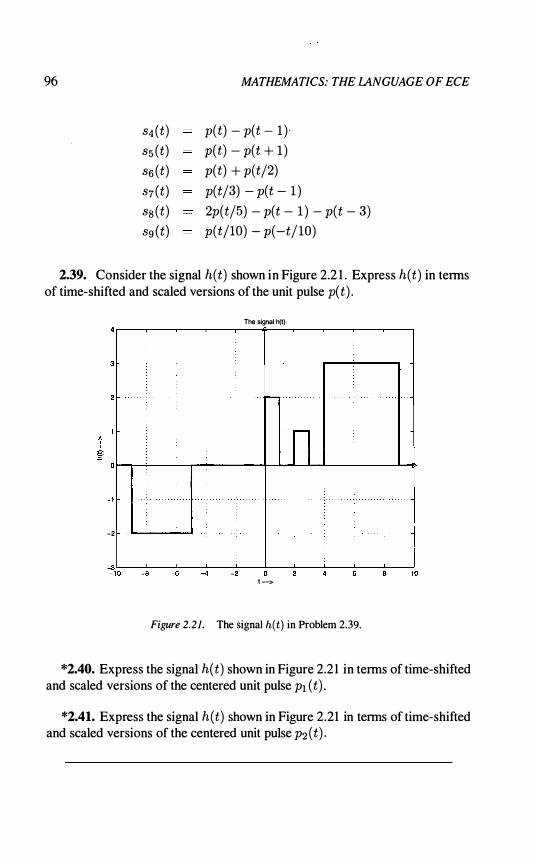
96
S4 (t) S5 (t) S6 (t) S7 (t) SS (t) sg (t)
MATHEMATICS: THE LANGUAGE OF ECE
p(t) - p(t - 1 ) ' p(t) - p(t + 1 ) p(t) + p(t/2) p(t/3) - p(t - 1 ) 2p(t/5) - p(t - 1 ) - p(t - 3) p(t/lO) - p(-t/lO)
2.39. Consider the signal h( t) shown in Figure 2.2 1 . Express h( t) in tenus of time-shifted and scaled versions of the unit pulse p( t) .
The signal h(l)
3
-2
��O --�_8---_76 --���-_�2 --�O�-7--�--�--7-�10 t -->
Figure 2.21. The signal h(t) in Problem 2.39.
*2.40. Express the signal h(t) shown in Figure 2.2 1 in tenus of time-shifted and scaled versions of the centered unit pulse PI (t) .
*2.41. Express the signal h(t) shown in Figure 2.21 in tenus of time-shifted and scaled versions of the centered unit pulse P2 (t) .
Signals in engineering 97
Problems you will see in other courses
This set of problems is intended to highl ight the connection of the material in this chapter to other ECE courses. The description of the problems is rather verbose, compared to the rest of the problems in thi s chapter. The problems are rather di fficult ; the main reason for that is the fact that (probably unfarn i l iar) technical concepts are now mixed with math, a language you have not had (yet) practiced sufficiently. Do not worry if you cannot tackle them at the first attempt. You wi l l sec these problems again, in the corresponding courses6 The purpose of putting them here i s to show you that the language we have just introduced is tightly connected to real istic ECE problems, studied in these more advanced courses. Hopefu lly, you wi l l find them more motivat i ng than the rest of the problems in this chapter. We wi l l revis i t such problems in later chapters, once we learn about Matlab, differential equat ions and transforms.
*2.42. (ECE301) The concept of convolution. The basis of ECE30 1 is the l inear, t ime-invariant system (e.g. , a circuit with constant R, L, C components). You wi l l learn about such systems in detail in ECE30 I . The input to such a system i s a s ignal x(t) (e.g. , a voltage source) ; the output i s another signal y(t )
(e .g . , the voltage across a capacitor) . In ECE30 1 , you wi l l prove a generic relationship that relates these two signals:
1+00 y(t ) = - 00 x(�)h(t - T)e (2 .49)
This is the celebrated con.volution integral. The function hU i s the impulse
response of the system. Our goal in this problem is to see how the convolution i ntegral can be eval
uated for some common signals described in this chapter.
Suppose that the input to this system is the signal
x(t ) = o( t ) ; (2.50)
we have d iscussed this signal in Section 2 . 1 .4 ( see Figure 2.8, in page 6 1 ) . Use Equation 2 . 1 8 to show that the output of the system i s the signal h(t)
(hence the name impulse response).
2 Let the input signal be a non-centered pulse of duration 2 t ime units, i .e . , let
x(t) = u(t - 1) - u(t - 3) . (2.5 1 )
6However. if you cannot tackle them at that time. you should worry :-)

98 MATHEMATICS: THE LANGUAGE OF ECE
Consider a system with an impulse response given by
h(t) = u(t) - u(t - 2) , (2.52)
another pulse-shaped signal . Determine the output of the system for each one of the following time instants:
t = - 10, - 1 , 0 , 1 , 2 , 3 , 4, 5, 6 , 10.
For example, when t = 1 , you must determine
J+OO y(l ) = -00 x(T)h(l - T)dT
This is' where you need the language we developed in this chapter: note that the signal h(l - T) appears to be time-shifted and time-reversed. You can evaluate this integral easily if you sketch the signals x( T) and h( 1 - T) and determine the area under their product.
3 Consider now the RC series circuit depicted in Figure 7. 1 , in page 33 1 , Chapter 7. For simplicity, suppose that R = 1 Ohm, and C = 1 Farad. The input to this system is the voltage source and the output is the voltage across the capacitor. In other words,
x(t) = lfs(t) , y(t) = Vc(t) .
In ECE301 , you will show that the impulse response of this system is
h(t) = e-tu(t) .
Suppose that the input to this RC circuit is the unit pulse in Equation 2. 1 2, page 59, with duration to = 2 time units; in other words, suppose that
x(t) = u(t) - u(t - 2) .
Show that the output of this RC circuit is given by { 0, t < 0, Vc (t) = 1 - e-t , ° � t < 2,
(e2 - l )e-t , 2 � t. (2.53)
You have already seen this output waveform in the ECE200 labs. Intuitively, the signal 1 - e-t describes how the capacitor is charged; the signal (e2 -1 )e-t describes how the capacitor is discharged.

Signals in engineering 99
4 Sketch the output given in Equation 2.53.
*2.43. (ECE303) Signals travelling on transmission lines. Consider a voltage source that is connected to a load (e.g. , a resistor) via a transmission line of length d meters. The source produces a signal v (t) . This signal (the electromagnetic energy of the signal , in ECE303 jargon) travels toward the load at the propagation velocity, vp, measured in meters/sec. This velocity depends on the type of the transmission line (e.g. , copper, fiber, coaxial cable, etc . ) We will use
vp = 2 . 108 meters/sec (2.54)
in this problem. This speed is about two thirds the speed of light in free space. To simplify presentation, consider a voltage source that produces a pulse of
duration 1 0 Ilsec; in other words, let
v (t } = u(t) - u(t - T) , where T = 10 . 10-6 seconds.
(2.55)
Because the propagation velocity is finite, the wave travelling from the source towards the load will not reach the load instantaneously. The time instant at which the rising edge of the pulse will be "felt" at the load depends of the length d of the transmission line.
An issue with transmission lines is losses. The line consumes some of the electromagnetic energy of the pulse, so what reaches the load is an attenuated and distorted version of the signal in Equation 2.55 . We will consider here "good quality lines", the loss less lines, for which the load receives an exact replica of the signal . Another issue with transmission lines is reflections. In a nutshell , once the electromagnetic energy of the pulse reaches the load, it gets reflected back towards the source, producing a wave (a voltage vr (t» that travels on the transmission line in the opposite direction. In ECE303, you will see that this reflection is given by
vr (t) = rL . v (t) , (2.56)
for some types of transmission lines and loads, not all . The constant r L is called the reflection coefficient and depends on the load characteristics . We can assume here that r L is a real number between 0 and 1 . Note that this reflected wave will reach the source and it may get reflected back towards the load one more time. This cycle can be repeated ad nauseam. For simplicity, here we will ignore this nuisance; in ECE303 you will consider ways to minimize reflection issues.
What exactly is happening on the transmission line? From this brief discussion, i t should be clear that the. summation of two voltages, v (t ) and vr (t) , is
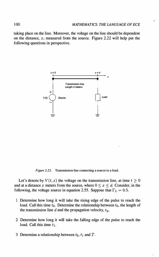
1 00 MATHEMATICS: THE LANGUAGE OF ECE
taking place on the line. Moreover, the voltage on the line should be dependent on the distance, x, measured from the source. Figure 2.22 will help put the following questions in perspective.
x = o I
+ V(t)
Transmission line, Length d meters
Source
x = d I x
Load
Figure 2.22. Transmission line connecting a source to a load.
Let's denote by V (t, x) the voltage on the transmission line, at time t :::=: a and at a distance x meters from the source, where 0 :S x :S d. Consider, in the following, the voltage source in equation 2.55 . Suppose that rL = 0. 5 .
Determine how long it will take the rising edge of the pulse to reach the load. Call this time to . Determine the relationship between to , the length of the transmission line d and the propagation velocity, vp .
2 Determine how long it will take the falling edge of the pulse to reach the load. Call this time tl .
3 Determine a relationship between to , tl and T.

Signals in engineering 1 0 1
4 Suppose that T < to . Detennine and sketch V(t, O ) , for 0 ::; t ::; to . Determine and sketch V(t, O) , for to ::; t ::; 2to . Detennine and sketch V(t, O ) , for 2to ::; t ::; 00.
5 Suppose that T < to . Detennine and sketch V(t, d) , for 0 ::; t ::; to . Determine and sketch V(t, d) , for to ::; t ::; to + T. Detennine and sketch V(t, d) , for to + T ::; t ::; 00.
6 Now consider a point on the line, at a distance x meters from the source. Determine and sketch V(t, x) , for t 2: o.
2.44. (ECE305) Transmission lines and three-phase AC voltages. Generation and transmission of electrical power is more efficient in electrical power systems consisting of two, or, more commonly, three sinusoidal voltages. You will investigate why in ECE305 .
The transmission lines that carry power from generation plants to residential areas have three cables that carry the following voltage wavefonns (called the three phases, a, b, c):
Vaal (t) Vbb' (t) vcc/ (t)
= V2V cos(271"60t) V2V cos(271"60t - 271"/3) V2V cos(271"60t - 471"/3)
(2.57)
(2.58)
(2.59)
In Equation 2.57, the subscripts a, a' refer to phase a. Equations 2.58 and 2.59 describe the voltages of phases b and c respectively. V is an amplitude parameter, that differs from transmission line to transmission line. It can range from a few hundred to thousands of Volts. From these equations, we can see that there is a phase difference of 271" /3 radians or 1200 between two "consecutive" phases.
Sketch the three wavefonns on the same graph, to see how they relate to each other.
2 Verify from this graph that the maximum voltage of phase b comes after (lags, in ECE305 jargon) that of phase a.
3 Rewrite Equation 2.58 in the fonn
Vbb' (t) = V2V cos(271"60(t - to) ) .
From this equation, figure out analytically how many seconds phase b lags phase a.
4 Rewrite the phase b voltage as a time-shifted version of the voltage Vaa' (t) .
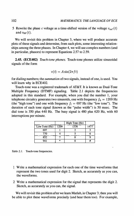
1 02 MATHEMATICS: THE LANGUAGE OF ECE
5 Rewrite the phase c voltage as a time-shifted version of the voltage Vaa' (t) and Vbb' (t) .
We will revisit this problem in Chapter 3 , where we will produce accurate plots of these signals and determine, from such plots, some interesting relationships among the three phases. In Chapter 4, we will use complex numbers (and in particular, phasors) to represent Equations 2.57 to 2.59.
2.45. (ECE402) Touch-tone phones. Touch-tone phones utilize sinusoidal signals of the form
V ( t) = A sin(27r ft)
for dialing numbers; the summation of two signals, instead of one, is used. You will learn why in ECE402.
Touch-tone was a registered trademark of AT&T. It is known as Dual-Tone Multiple Frequency (DTMF) signaling. Table 2. 1 depicts the frequencies adopted in this standard. For example, when you dial the number 1 , your telephone circuitry generates two sinusoids, one with frequency !h = 1209 Hz (the "high tone") and one with frequency fl = 697 Hz (the "low tone") . The duration of each tone signal (known as the "pulse width") is 50 msec. The dial tone is 350 plus 440 Hz. The busy signal is 480 plus 620 Hz, with 60 interruptions per minute.
High Tone (Hz)
Low Tone (Hz) 1 209 1336 1 477
697 1 2 3
770 4 5 6
852 7 8 9
94 1 * 0 #
Table 2. 1 . Touch-tone frequencies.
Write a mathematical expression for each one of the time waveforms that represent the two tones used for digit 2. Sketch, as accurately as you can, the waveforms.
2 Write a mathematical expression for the signal that represents the digit 2. Sketch, as accurately as you can, the signal .
We will revisit this problem after we learn Matlab, in Chapter 3 ; then you will be able to plot these waveforms precisely (and hear them too). For example,
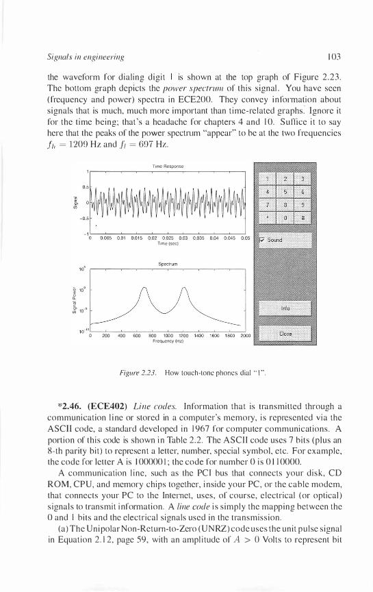
Signals in engineering 1 03
the waveform for dial ing digit is shown at the top graph of Figure 2 .23 . The bottom graph depicts the power spectrum of th is signal . You have seen (frequency and power) spectra in ECE200. They convey infOlmation about signals that is much, much more important than t ime-related graphs� Ignore it for the t ime being; that 's a headache for chapters 4 and 1 0. Suffice i t to say here that the peaks of the power spectrum "appear" to be at the two frequencies
.fh = 1209 Hz and It = 697 Hz.
Time Response
-'o�-=-0.00==-5 -:0":-.0"'1 -:0-:'.0 1:::-5----=-'0.0=2--::c0.0:':"25:--::0-':c.03:--::-:'=-:-':-:--�,...--:-' Time (sec)
! 10° Q.
� � 10-5
10- IO,--�_��_�_��_��_�----, o 200 400 600 800 1000 1200 Frequency (Hz)
Figure 2.23. How louch-lone phones dial " 1 ".
*2.46. (ECE402) Line codes. Information that is transmitted through a communication l i ne or stored in a computer's memory, i s represented via the ASCII code, a standard developed in 1 967 for computer communications. A portion of this code is shown i n Table 2.2 . The ASCII code uses 7 bits (plus an 8-th parity bit) to represent a letter, number, special symbol, etc. For example, the code for letter A is 1 00000 I ; the code for number 0 i s 0 1 1 0000.
A communication l ine, such as the PCl bus that connects your disk, CD ROM, CPU, and memory chips together, i nside your PC, or the cable modem, that connects your PC to the Internet, uses, of course, e lectrical (or optical ) s ignals to transmit i nformation. A line code i s simply the mapping between the o and 1 bits and the electrical signals used in the transmission.
(a) The Unipolar Non-Return-to-Zero (UNRZ) code uses the unit pulse signal in Equation 2 . 1 2, page 59, with an ampl i tude of A > 0 Volts to represent bit
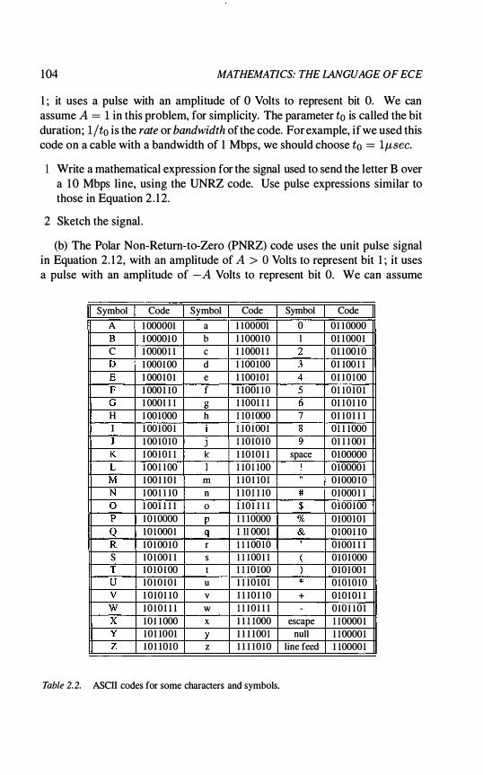
104 MATHEMATICS: THE LANGUAGE OF ECE
1 ; it uses a pulse with an amplitude of 0 Volts to represent bit O. We can assume A = I in this problem, for simplicity. The parameter to is called the bit duration; lito is the rate or bandwidth of the code. For example, if we used this code on a cable with a bandwidth of 1 Mbps, we should choose to = lp,sec.
Write a mathematical expression for the signal used to send the letter B over a 1 0 Mbps line, using the UNRZ code. Use pulse expressions similar to those in Equation 2. 1 2.
2 Sketch the signal .
(b) The Polar Non-Retum-to-Zero (PNRZ) code uses the unit pulse signal in Equation 2. 1 2, with an amplitude of A > 0 Volts to represent bit 1 ; it uses a pulse with an amplitude of -A Volts to represent bit O. We can assume
II Symbol I Code I Symbol I Code I Symbol I Code
A 1 000001 a 1 1 00001
B 1 00001 0 b 1 1 000 1 0
C 1 0000 1 1 c 1 1 000 1 1
D 1 0001 00 d 1 100100
E 1 000 1 0 1 e 1 1001 0 1
F 1 000 1 1 0 f 1 1001 1 0
G 1 0001 1 1 g 1 1001 1 1
H 1 00 1 000 h 1 10 1 000
I 1 00 1 00 1 i 1 1 0 1 001
J 1 00 1 0 1 0 j 1 10 1 0 1 0
K 1 00 1 0 1 1 k 1 1 0 1 0 1 1
L 1 00 1 1 00 I 1 10 1 1 00
M 1 00 1 1 0 1 m 1 1 0 1 1 0 1
N 1 00 1 1 1 0 n 1 1 0 1 1 1 0
0 1 001 1 1 1 0 1 10 1 1 1 1
P 1 0 1 0000 P l l l OOOO
Q 1 0 1 0001 q 1 11 0001
R 1 0 1 00 1 0 r I l l OO I O
S 1 0 1 00 1 1 s I l l OO 1 1
T 1 0 1 0 1 00 t 1 1 1 0 1 00
U 1 0 1 0 1 0 1 u 1 1 1 0 1 0 1
V 1 0 1 0 1 1 0 v 1 1 1 0 1 1 0
W 1 0 1 0 1 1 1 w 1 1 1 0 1 1 1
X 1 0 1 1 000 x 1 1 1 1000
y 1 0 1 1001 Y 1 1 1 1 00 1
Z 1 0 1 1 0 1 0 z 1 1 1 1 0 1 0
Table 2.2. ASCII codes for some characters and symbols.
0 01 1 0000
I 01 1 0001
2 01 1 00 1 0
3 01 100 1 1
4 01 1 0 1 00
5 01 1 0 1 0 1
6 01 1 01 1 0
7 01 1 0 1 1 1
8 01 1 1 000
9 01 1 1 00 1
space 01 00000
! 010000 1 "
01000 1 0
# 01000 1 1
$ 0100 1 00
% 0100 1 0 1
& 0 1 O01 l 0 ,
01001 1 1
( 0 1 0 1 000
) 0 1 0 1 00 1 * 0 1 0 1 0 1 0
+ 0 1 0 1 0 1 1 - 010 1 1 0 1
escape 1 1 0000 1
null 1 1 0000 1
line feed 1 10000 1
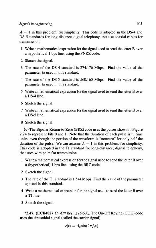
Signals in engineering 1 05
A = 1 in this problem, for simplicity. This code is adopted in the DS-4 and DS-5 standards for long-distance, digital telephony, that use coaxial cables for transmission.
Write a mathematical expression for the signal used to send the letter B over a hypothetical 1 bps line, using the PNRZ code.
2 Sketch the signal .
3 The rate of the DS-4 standard is 274. 1 76 Mbps. Find the value of the parameter to used in this standard.
4 The rate of the DS-5 standard is 560. 1 60 Mbps. Find the value of the parameter to used in this standard.
5 Write a mathematical expression for the signal used to send the letter B over a DS-4 Iine.
6 Sketch the signal .
7 Write a mathematical expression for the signal used to send the letter B over a DS-5 1ine.
8 Sketch the signal .
(c) The Bipolar Return-to-Zero (BRZ) code uses the pulses shown in Figure 2.24 to represent bits 0 and 1 . Note that the duration of each pulse is to time units, even though the portion of the waveform is "nonzero" for only half the duration of the pulse. We can assume A = 1 in this problem, for simplicity. This code is adopted in the TI standard for long-distance, digital telephony, that uses wire pairs for transmission.
1 Write a mathematical expression for the signal used to send the letter B over a (hypothetical) 1 bps line, using the BRZ code.
2 Sketch the signal.
3 The rate of the TI standard is 1 .544 Mbps. Find the value of the parameter to used in this standard.
4 Write a mathematical expression for the signal used to send the letter B over a T I line.
5 Sketch the signal .
*2.47. (ECE402) On-Off Keying (OOK). The On-Off Keying (OOK) code uses the sinusoidal signal (called the carrier signal)
c(t) = Ac sin(27rfct )
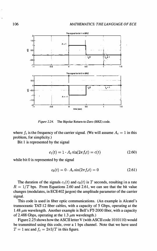
1 06 MATHEMATICS: THE lANGUAGE OF ECE
1 .5
� 0.5
o
-0.5
-1 -1
0.5
i -0.5
1
-1 .5
2 -1
The signal for bit 1 in SRZ
A = l
1012
-0.5 0.5
The signal for bit 0 in BRZ
. . . I 1012
A = -l
-0.5 0.5 time (sec)
. " , to r 1
10 = 1
Figure 2.24. The Bipolar Return-to-Zero (BRZ) code.
1 .5
1 .5
where Ie is the frequency of the carrier signal. (We will assume Ae = 1 in this problem, for simplicity. )
Bit 1 is represented by the signal
(2.60)
while bit 0 is represented by the signal
co (t) = O · Ae sin(27rIet) = 0 (2.6 1 )
The duration of the signals Cl (t) and co (t) is T seconds, resulting i n a rate R = liT bps. From Equations 2.60 and 2.6 1 , we can see that the bit value changes (modulates, in ECE402 jargon) the amplitude parameter of the carrier signal .
This code is used in fiber optic communications. (An example is Alcatel 's transoceanic TAT- 1 2 fiber cables, with a capacity of 5 Gbps, operating at the 1 .48 pm wavelength. Another example is Bell 's FT-2000 fiber, with a capacity of 2.488 Gbps, operating at the 1 .3 pm wavelength.)
Figure 2.25 shows how the ASCII letter V (with ASCII code 1 0 10 1 1 0) would be transmitted using this code, over a 1 bps channel . Note that we have used T = 1 sec and Ie = 27r31T in this figure.

Signals in engineering 1 07
Let Ie = 1 / (2T) . Sketch the wavefonn transmitted over an Ff-2000 fiber, for the letter B. Be sure to mark your horizontal axis accurately.
2 The ECE220 textbook is about 3.5 Mbytes long (in PDF fonnat) . How long would it take to transmit it over a TAT- 1 2 fiber cable?
1 .5
� 0.5
-0.5
The laner V in ASCII code
6T 7T
_1 � __ � __ -L __ -J ____ L-__ J-__ -L __ � ____ � __ � -1
� 0
-1
-2 -1
The signal tor letter V in OOK
1 o I 1 o � 1 1
� V � . 3
time (sec)
Figure 2.25. The On-Off Keying (OOK) code.
0
*2.48. (ECE402) Binary Phase Shift Keying (BPSK). The Binary Phase Shift Keying (BPSK) code uses the sinusoidal carrier signal
where Ie is the frequency of the carrier signal . (We will assume Ae = 1 in this problem, for simplicity. )
Bit 1 is represented by the signal
Cl (t) = Ae sin(27rfet + 1 · 7r)
while bit 0 is represented by the signal
co (t) = Ae sin(27rIet + O · 7r) = c(t)
(2.62)
(2.63)
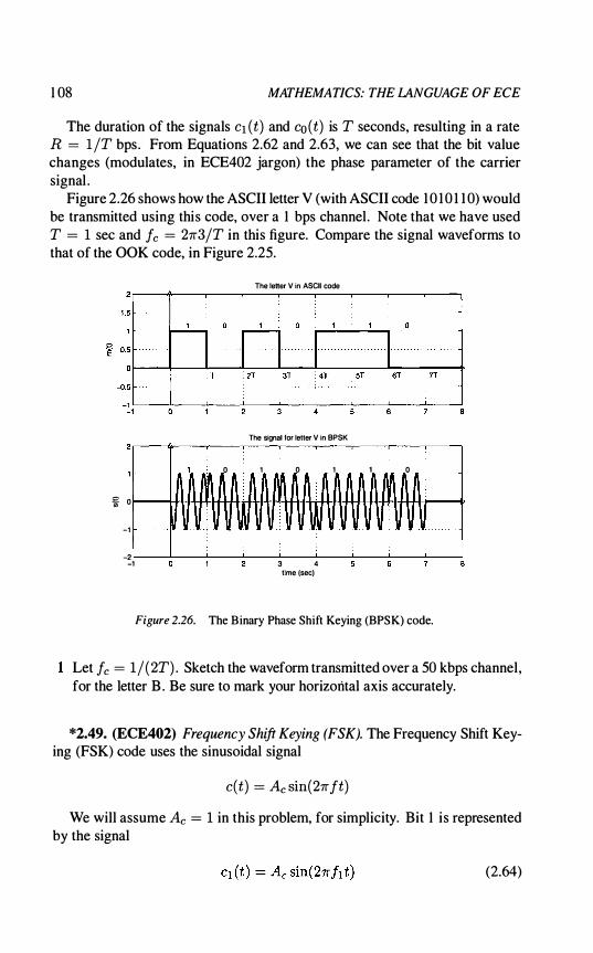
1 08 MATHEMATICS: THE LANGUAGE OF ECE
The duration of the signals Cl (t) and co (t) is T seconds, resulting in a rate R = l /T bps. From Equations 2.62 and 2.63, we can see that the bit value changes (modulates, in ECE402 jargon) the phase parameter of the carrier signal .
Figure 2.26 shows how the ASCII letter V (with ASCII code 1 0 1 0 1 1 0) would be transmitted using this code, over a I bps channel . Note that we have used T = 1 sec and Ie = 27f3/T in this figure. Compare the signal waveforms to that of the OOK code, in Figure 2.25.
� 0
-1
-2 -1
1 M 0
W
The leHer V in ASCII code
The signal for letter V in BPSK
1 � 0
� 3 4
time (sec)
1 1 M 0
V
Figure 2.26. The Binary Phase Shift Keying (BPSK) code.
Let Ie = 1/ (2T) . Sketch the waveform transmitted over a 50 kbps channel , for the letter B . Be sure to mark your horizontal axis accurately.
*2.49. (ECE402) Frequency Shift Keying (FSK). The Frequency Shift Keying (FSK) code uses the sinusoidal signal
c(t) = Ae sin(27fIt)
We will assume Ae = 1 in this problem, for simplicity. Bit I is represented by the signal
(2.64)

Signals in engineering 1 09
while bit 0 is represented by the signal
(2.65 )
fo and h are two distinct frequencies. The duration of the signals c} ( t ) and co (t) is T seconds, resulting in a rate R = liT bps. The way a sequence of bits, say 1 0 1 , is encoded into a signal c( t) , can be explained by the following example: { c} ( t ) , 0 � t < T,
c(t) = co (t ) , T � t < 2T, c} (t) , 2T � t < 3T ,
From Equations 2.64 and 2.65 , we can see that the bit value changes (modulates, in ECE402 jargon) the frequency parameter of the carrier signal . This code was used, among other applications, in low-speed modems, such as the Bell-type 1 03 modem. The rate of this modem was 300 bps, indeed low, by today's standards. The frequencies selected in this standard were h = 1270 Hz, fo = 1070 Hz, for the originating modem (i.e., the one that initiated the communication); for the answering modem, the frequencies were h = 2225 Hz and fo = 2025 Hz. Separate originating/answering frequencies were selected to enable bidirectional (in ECE402 jargon,full-duplex) communication.
Figure 2.27 shows how the ASCII letter V (with ASCII code 1 0 1 0 1 1 0) would be transmitted using this code, over a 1 kbps channel . Note that T = 1 msec for such a channel . Compare the signal waveforms to those of the OOK and BPSK codes, in Figures 2.25 and 2.26.
Write a mathematical expression for the signal used to send the letter B over a (hypothetical) 1 bps line, using the FSK code. Observe from Figure 2.27 that the transmitted signal is not continuous. Make sure your equation captures this discontinuity. Use Equations 2.64 and 2.65 to explain this discontinuity. Use the answering Bell-type 1 03 modem frequencies.
2 Sketch the waveform transmitted over a 300 bps channel , for the letter B . Use the originating Bell-type 1 03 modem frequencies. Be sure to mark your horizontal axis accurately.
*2.50. (ECE420) Time-shifting. An antenna located in New York, USA, transmits signals to an antenna in London, UK. The signals are transmitted via a geostationary satellite (i .e . , one that stays in a fixed location approximately L � 22, 300 miles from the surface of the earth). The Inte1sat VI, launched in 1 986, is a geostationary satellite; it uses a 6 GHz channel towards the satellite and a 4 GHz channel from the satellite to the earth stations.
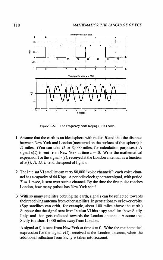
1 1 0 MATHEMATICS: THE LANGUAGE OF ECE
The letter V in ASCII code
1 .5
f 0.5
7T -0.5
-�lL __ � ____ L-__ � __ � __ � __ �� __ � __ � __ �
The signal for letter V in FSK
-1
�1L---�--�--�--�3�--�4 --��--7---�--� 1 (msec)
Figure 2.27. The Frequency Shift Keying (FSK) code.
1 Assume that the earth is an ideal sphere with radius R and that the distance between New York and London (measured on the surface of that sphere) is D miles. (You can take D :::::: 3, 000 miles, for calculation purposes.) A signal s(t) is sent from New York at time t = O. Write the mathematical expression for the signal r(t) , received at the London antenna, as a function of s(t) , R, D, L, and the speed of l ight c.
2 The Intelsat VI satellite can carry 80,000 "voice channels" ; each voice channel has a capacity of 64 Kbps. A periodic clock generator signal , with period T = 1 msec, is sent over such a channel. By the time the first pulse reaches London, how many pulses has New York sent?
3 With so many satellites orbiting the earth, signals can be reflected towards their receiving antenna from other satellites, in geostationary or lower orbits. (Spy satellites can orbit, for example, about 1 00 miles above the earth. ) Suppose that the signal sent from Intelsat VI hits a spy satellite above Sicily, Italy, and then gets reflected towards the London antenna. Assume that Sicily is a short 1 ,000 miles away from London.
A signal s(t) is sent from New York at time t = o. Write the mathematical expression for the signal r(t) , received at the London antenna, when the additional reflection from Sicily is taken into account.
Signals in engineering I I I
*2.51. (ECE421) Sampling of analog signals. Analog signals, such as voice, are very often converted to digital ones, so that, for example, they can be processed via a computer or specialized hardware, like an ASIC or FPGA. An analog voltage signal , for example, can have continuous values, such as all values in the interval [0 , 1 ] Volts. A discrete voltage signal, on the other hand, can only have discrete values, such as all values in the interval {O, 0 .25 , 0 . 5 , 0.75, 1 } Volts. Analog-to-Digital (AD) converters can be used to perform conversion of an analog signal, such as
Va(t) = sin(27rIt) (2.66)
into a digital one. There are many ways this conversion can take place. A commonly used one is to sample the analog signal periodically, with a frequency Is (or, equivalently, with a period Ts = 1/ Is) . The digital signal is then represented by the sequence of values
(2.67)
Note that the digital signal is not defined for times other than the sampling instants kTs .
Consider the signal in Equation 2.66. Let I = 1 , and suppose that the domain is equal to 4 periods; in other words, t E [0, 4) . Determine the range of values for this analog signal . Sketch this signal over the entire domain.
2 Suppose that the sampling frequency is equal to the frequency of the signal in Equation 2.66, i.e. , let Is = I (= 1 ) . Sampling starts at t = O. Determine all possible values that the digital signal can take. Any surprises?
3 Suppose now that the sampling frequency is equal to Is = 81 (= 8) . Determine all possible values that the digital signal can take. Sketch the digital signal. Clearly mark your horizontal axis .
4 Consider a generic sampling frequency Is . Determine the domain (not the range ! ) of the digital signal . Is it the same as the domain of the analog signal? Why?
5 Consider a new signal , call it Vd(t) , that has the same domain as the analog signal va (t) . The signal Vd(t) is defined as follows:
if t is a sampling instant (t = kTs for some an k) otherwise.
(2.68)

1 1 2 MATHEMATICS: THE LANGUAGE OF ECE
6 Sketch this signal .
7 What is the relationship of this signal and the digital signal we described in Equation 2.67?
8 Sketch the abstruse signal
00
j(t) = L J(t - kTs ) k=O
9 In ECE421 jargon, this signal is called an impulse train. Explain, using this sketch, why.
l O In the same jargon, this signal is also called a comb, at least by ECE engineers whose artistic side is not entirely suppressed by endless math. Explain, using the same sketch, Why.
1 1 Consider one more new signal, call it v,,( t) , that has the same domain as the analog signal va (t) . The signal v,,(t) is defined as follows:
00
v,, (t) = L va(t)J(t - kTs ) (2.69) k=O
Sketch the signal in Equation 2.69, when va (t) is given by Equation 2.66.
12 What is the relationship of this signal and the digital signal that we described in Equation 2.67?
13 Equation 2 .69 is a #@%&! mathematical formula that can be used to describe the digital signal . Equation 2.67 also describes the essential information about the digital signal ; however it is just a bunch of numbers. Do you see any (big) advantage in using a (not so intuitive, difficult) formula like Equation 2.69, versus using easy to understand, intuitive numbers, like Equation 2.67?

Chapter 3
MATLAB PROGRAMMING
Matlab is a powerful, widely used computation and graphics package. Computations in Matlab can be done numerically or symbolically. The syntax of the Matlab language is similar to that of the C programming language.
This chapter is not intended to be a Matlab manual; it does not provide the full syntax and/or capabilities of the described Matlab commands. Our main focus is computation and (two-dimensional) plotting of signals; therefore, in
. this chapter we introduce only the Matlab commands that we will need to: (a) define a signal , and, (b) plot it. Additional Matlab commands will be introduced in later chapters, on an as needed basis. At the end of this chapter, you should be able to write a complete Matlab program (we call such programs scripts) to calculate and plot any signal that we described in Chapter 2, especially the periodic ones.
1. Defining a signal in Matlab
Recall that a signal is represented by a function J(x) . For signals where x is continuous time, we will use the notation J(t) ; for signals where x is discrete time, we will use the notation J (n) . For the purposes of this chapter, the argument of the function will be interpreted as time. The range of values that x can take will be called the time domain.
Consider the signal
J (t) = sin(27rt ) .
Suppose we are interested in evaluating this signal for t E [- 10 , 20] . In order to represent this signal in Matlab, the time domain must be defined first. Note that the domain [-10, 20] contains an infinite number of elements. Representing all of them is not possible (in Matlab or any other computer language, for that
1 1 3

1 14 MATHEMATICS: THE lANGUAGE OF ECE
.. matter), since it would require an infinite amount of memory. An approximation (called a discretization of the continuous time interval) is necessary. For example, some possible discretizations include the following:
T1 T2 T3
{- 1O -9 -8 . . . - 1 ° 1 . . . 19 20} , , , , ' " , , { - 10.0, -9.9, -9.8 , . . . , -0. 1 , 0, 0 . 1 , · . . , 19 .9, 20.0} { - 1O.00, -9.99, -9.98, · . . , -0.01 , 0, 0.0 1 , . . . , 19.99 , 20.00}
In Matlab the above time domains can be represented with the Matlab commands:
T1 - 10 T2 - 10 T3 -10
1 : 20 ; 0 . 1 : 20 ; 0 . 01 : 20 ;
In the above commands, the symbols T1, T2, T3 are called Matlab variables. All three commands are special cases of assignment commands; they assign values (whatever appears on the right of the = sign) to the variables (whatever appears on the left of the = sign). In the notation - 1 0 : 1 : 20, - 1 0 is the lower value; 1 is the discretization step; 20 is the upper value. The ; at the end of the assignment command is the output suppressor. When you execute the command
T l = -10 : 1 : 20 ;
through the Matlab window on your computer, nothing appears on your screen. When you execute the command
Tl = -10 : 1 : 20
through the Matlab window on your computer, you will see a list of all the values assigned to the variable Tl .
Once a time domain has been defined, a signal over this domain can be easily defined, using an assignment statement of the form
variable_name = signal_value ;
The following examples demonstrate a few ways. In order to make the examples more readable, we introduce some comments before the actual Matlab code. Comments in Matlab always start with the % sign and end at the end of the line. Comments can be in a line by themselves or at the end of a command.
Example 3.1. Let f(t) = t, where t E [0, 10] . Let's use a discretization step of 0.5, in representing the time domain. A Matlab program that evaluates f (t) over this interval is the following:
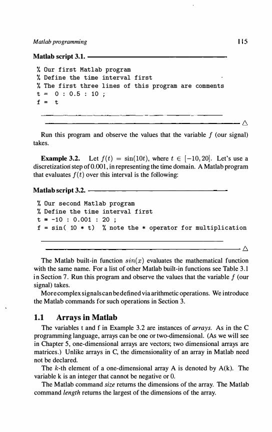
Matlab programming
Matlab script 3.1. -----------------,
% Our f irst Matlab program % Def ine the t.ime interval f irst % The f irst three lines of this program are comments t o : 0 . 5 : 10 f = t
1 1 5
---------------------------------------------- 6 Run this program and observe the values that the variable f (our signal)
takes.
Example 3.2. Let f(t) = sin( lOt ) , where t E [-10, 20] . Let's use a discretizatiori step of 0.00 1 , in representing the time domain. A Matlab program that evaluates f(t) over this interval is the following:
Matlab script 3.2. ------------------
% Our second Matlab program % Def ine the t ime interval f irst t - 1 0 : 0 . 00 1 : 20 ; f = s in e 10 * t ) % note the * operator f or multipli c ation
-------------------------------------------- 6 The Matlab built-in function sin(x) evaluates the mathematical function
with the same name. For a list of other Matlab built-in functions see Table 3 . 1 i n Section 7 . Run this program and observe the values that the variable f (our signal) takes.
More complex signals can be defined via arithmetic operations. We introduce the Matlab commands for such operations in Section 3 .
1.1 Arrays in Matlab
The variables t and f in Example 3 .2 are instances of arrays. As in the C programming language, arrays can be one or two-dimensional . (As we will see in Chapter 5 , one-dimensional arrays are vectors; two dimensional arrays are matrices . ) Unlike arrays in C, the dimensionality of an array in Matlab need not be declared.
The k-th element of a one-dimensional array A is denoted by A(k). The variable k is an integer that cannot be negative or O.
The Matlab command size returns the dimensions of the array. The Matlab command length returns the largest of the dimensions of the array.

1 1 6 MATHEMATICS: THE LANGUAGE OF ECE
Example 3.3. Consider the commands
Matlab script 3.3. -----------------,
t l = 1 : 2 : 7 size (t l ) length (t l ) a = t l ( 1 )
The variable t l i s an array with 4 elements, namely 1 , 3 , 5 , and 7 . The first element of the array, t l ( 1 ) , is equal to I ; t l (2) is equal to 3 ; t 1 (3) is equal to 5 ; t 1 (4) is equal to 7 . The size command returns two values, 1 and 4. These values indicate that t 1 has one row and 4 columns (more on that in Chapter 5) . The length of t 1 is 4. The command a = t I ( 1 ) assigns the value 1 to the variable a. ----------------------- 6
2. Plotting
Accurate signal plots are invaluable in engineering; they provide insight into the signal behavior and facilitate study of their properties. Matlab is an excellent tool for signal plotting. It provides a wealthy set of commands to generate, and further process plots.
2.1 Commands for two-dimensional plots
In this section we will introduce the basic Matlab commands for creating two-dimensional plots, i .e . , for plotting a signal f(t) versus its argument t.
2.1.1 What is a good plot? A "good" two-dimensional plot should provide all the information needed
to describe the signal . It consists of the following elements:
An "accurate " plot of the signal. Clearly, if the plot is inaccurate, information about the signal and its properties is lost. The discretization of the time domain is the parameter that mostly affects the accuracy of the plot, as figures 3.2, page 1 2 1 and 3.3 , page 1 22, demonstrate. Another parameter that also affects plotting accuracy is the amount of data, as Figure 3 .4, page 1 23, demonstrates. If the function is "smooth", the, plot should appear smooth as well . If the function is periodic, the plot should show enough periods to indicate periodicity ; three to four periods with about twenty to thirty samples per period is usually sufficient.
2 A clearly labelled horizontal axis. A label identifying the name of the independent variable (and its units) is always helpful.
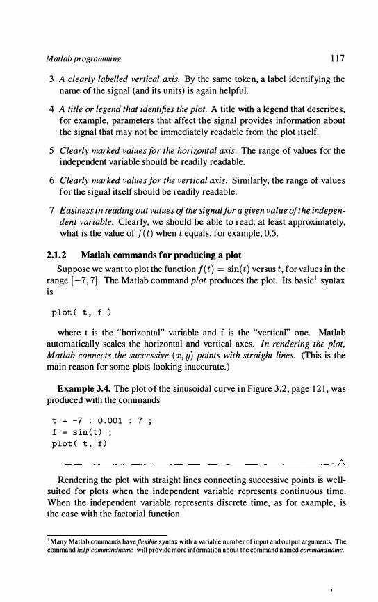
Matlab programming 1 1 7
3 A clearly labelled vertical axis. By the same token, a label identifying the name of the signal (and its units) is again helpful .
4 A title or legend that identifies the plot. A title with a legend that describes, for example, parameters that affect the signal provides information about the signal that may not be immediately readable from the plot itself.
5 Clearly marked values for the horizontal axis. The range of values for the independent variable should be readily readable.
6 Clearly marked values for the vertical axis. Similarly, the range of values for the signal itself should be readily readable.
7 Easiness ill reading out values of the signalfor a given value of the independent variable. Clearly, we should be able to read, at least approximately, what is the value of f(t) when t equals, for example, 0.5 .
2.1.2 Matlab commands for producing a plot Suppose we want to plot the function f(t) = sin(t) versus t, for values in the
range [-7, 7] . The Matlab command plot produces the plot. Its basic I syntax is
plot ( t , f )
where t is the "horizontal" variable and f is the "vertical" one. Matlab automatically scales the horizontal and vertical axes. In rendering the plot, Matlab connects the successive (x, y) points with straight lines. (This is the main reason for some plots looking inaccurate. )
Example 3.4. The plot of the sinusoidal curve in Figure 3 .2 , page 1 2 1 , was produced with the commands
t = -7 : 0 . 00 1 : 7 ; f = s in (t) ; plot ( t , f )
--------------------------------------------- 6 Rendering the plot with straight lines connecting successive points is well
suited for plots when the independent variable represents continuous time. When the independent variable represents discrete time, as for example, is the case with the factorial function
I Many Matlab commands have flexible syntax with a variable number of input and output argumenls. The command help commandllame will provide more information about the command named commandname.
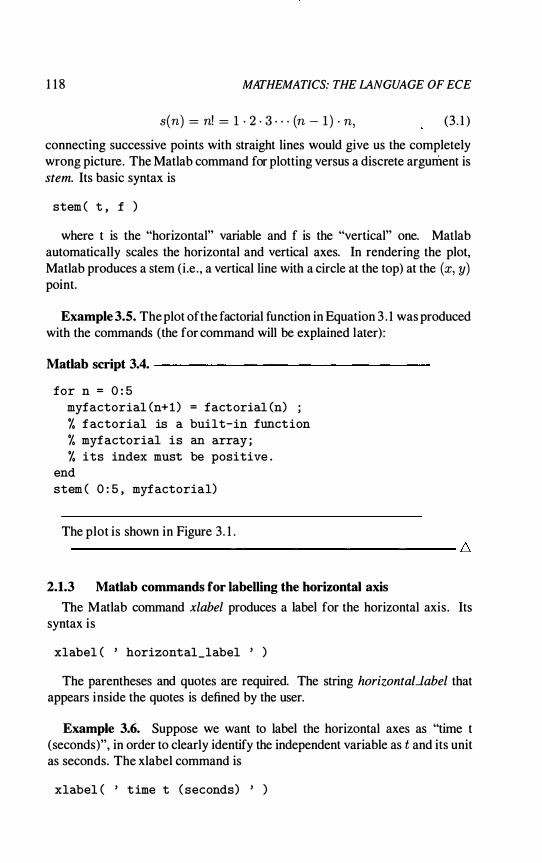
1 1 8 MATHEMATICS: THE LANGUAGE OF ECE
s(n) = n! = 1 · 2 · 3 · · · (n - 1 ) . n, (3 . 1 )
connecting successive points with straight lines would give us the completely wrong picture. The Matlab command for plotting versus a discrete argument is stem. Its basic syntax is
stem ( t , f )
where t is the "horizontal" variable and f is the "vertical" one. Matlab automatically scales the horizontal and vertical axes. In rendering the plot, Matlab produces a stem (i.e . , a vertical line with a circle at the top) at the (x, y) point.
Example 3.5. The plot of the factorial function in Equation 3 . 1 was produced with the commands (the for command will be explained later) :
Matlab script 3.4. -----------------
for n = 0 : 5 myfactorial (n+ 1 ) = factorial (n) ; % f actorial is a built-in function % myfactorial is an array ; % its index must be positive .
end stem ( 0 : 5 , myfactorial)
The plot is shown in Figure 3 . 1 . -------------------------------------------- 6
2.1.3 Matlab commands for labelling the horizontal axis The Matlab command xlabel produces a label for the horizontal axis . Its
syntax is
xlabel ( , horizontal_label ' )
The parentheses and quotes are required. The string horizontaL/abel that appears inside the quotes is defined by the user.
Example 3.6. Suppose we want to label the horizontal axes as "time t (seconds)", in order to clearly identify the independent variable as t and its unit as seconds. The xlabel command is
xlabel ( , t ime t ( seconds) , )

Matiah programming
The factorial function 1 20r--,----,----.---.---,---.----,-----.--..,----�
1 00
80
" 60
40
20
0.5 3.5 n -->
Figure 3. 1 . Plot of the factorial function.
4.5
1 1 9
--------------------------------------------- 6
Example 3.7. The horizontal label for the plot in Figure 3.2, page 1 2 1 , was produced with the command
xlabel ( , t - -> (msec) , )
2.1.4 Matlab commands for labelling the vertical axis The MatIab command ylabel produces a label for the vertical axis. Its syntax
is
ylabel ( , vertical_label ' )
The parentheses and quotes are required. The string verticaUabel that appears inside the quotes is defined by the user.
Example 3.8. The vertical label for the plot in Figure 3.2, page 1 2 1 , was produced with the command
ylabel ( , f (t ) - - > (Volts ) , )
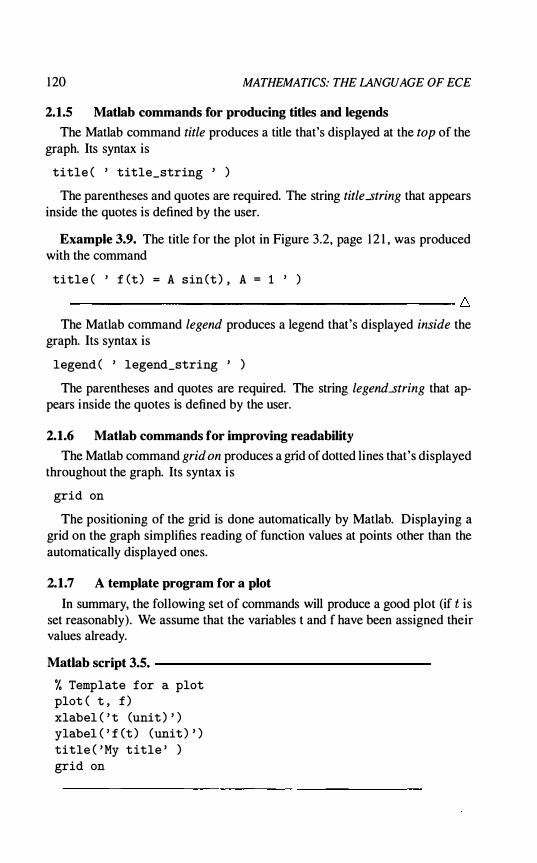
1 20 MATHEMATICS: THE LANGUAGE OF ECE
2.1.5 Matlab commands for producing titles and legends The Matlab command title produces a title that's displayed at the top of the
graph. Its syntax is
title ( , title_string , )
The parentheses and quotes are required. The string title...string that appears inside the quotes is defined by the user.
Example 3.9. The title for the plot in Figure 3.2, page 1 2 1 , was produced with the command
title ( , f (t ) = A sin (t ) , A = 1 ' )
-------------------------------------------- 6 The Matlab command legend produces a legend that's displayed inside the
graph. Its syntax is
legend ( , legend_string , )
The parentheses and quotes are required. The string legend...string that appears inside the quotes is defined by the user.
2.1.6 Matlab commands for improving readability The Matlab command grid on produces a grid of dotted lines that's displayed
throughout the graph. Its syntax is
grid on
The positioning of the grid is done automatically by Matlab. Displaying a grid on the graph simplifies reading of function values at points other than the automatically displayed ones.
2.1.7 A template program for a plot In summary, the following set of commands will produce a good plot (if t is
set reasonably). We assume that the variables t and f have been assigned their values already.
Matlab script 3.5. ------------------,
% Template for a plot plot ( t , f ) xlabel ( ' t (unit ) ' ) ylabel ( ' f (t ) (unit ) ' ) title ( ' My t itle ' ) grid on
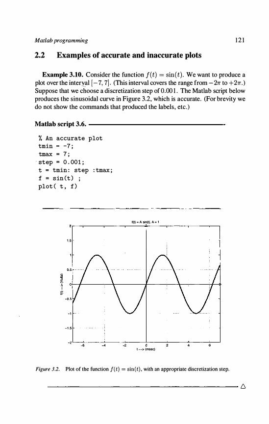
Matlab programming 1 2 1
2.2 Examples of accurate and inaccurate plots
Example 3.10. Consider the function f(t) = sin(t) . We want to produce a plot over the interyal [- 7, 7] . (This interval covers the range from - 27r to + 27r. ) Suppose that we choose a discretization step of 0.00 1 . The Matlab script below produces the sinusoidal curve in Figure 3.2, which is accurate. (For brevity we do not show the commands that produced the labels, etc . )
Matlab script 3.6. -----------------
% An accurate plot tmin -7 ; tmax = 7 ;
. step = 0 . 00 1 ; t = tmin : step : tmax ; f = s in (t ) ; plot ( t , f )
1 .5
-1 .5
fIt) = A sin(t). A = ,
-2L-�_6L---�_4------�2----�O-----L-----L-----L�
t --> (msee)
Figure 3.2. Plot of the function f(t) = sin(t) . with an appropriate discretization step.
-------------------------------------------- 6
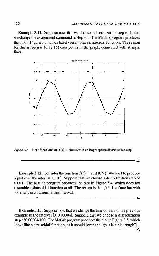
1 22 MATHEMATICS: THE lANGUAGE OF ECE
Example 3.11. Suppose now that we choose a discretization step of 1 , i .e . , we change the assignment command to step = 1 . The Matlab program produces the plot in Figure 3 .3 , which barely resembles a sinusoidal function. The reason for this is too few (only 1 5) data points in the graph, connected with straight lines.
1(1) = A sin(I). A = 1
1 .5
-1 .5
_2' L--L __ -'-__ --'-__ ..l.-__ -'----__ '-__ L----l -6 -4 -2 o
1 ->
Figure 3.3. Plot of the function f(t) = sin(t) , with an inappropriate discretization step.
--------------------------------------------- 6
Example 3.12. Consider the function f (t) = sin( 106t ) . We want to produce a plot over the interval [0, 10] . Suppose that we choose a discretization step of 0.00 1 . The Matlab program produces the plot in Figure 3 .4, which does not resemble a sinusoidal function at ail . The reason is that f(t) is a function with too many oscillations in this interval . ------------------------------------------ 6
Example 3.13. Suppose now that we change the time domain of the previous example to the interval [0, 0 .00004] . Suppose that we choose a discretization step of 0.000041 1 00. The Matlab program produces the plot in Figure 3.5, which looks like a sinusoidal function, as it should (even though it is a bit "rough"). ------------------------------------------ 6

Matlab programming
1(1) = sin( 10"t)
1 .5
0.5 J!l "0 ;::. � 0 I
g -D.5
-I
-1.5
-2 0 10
t -->
Figure 3.4. Plot of the function f(t) = sin( 106t) . over an inappropriate interval.
1(1) = sin(1 06,)
1 .5
-1 .5
-20�--�0�.5----
-L----�1�.5----�----�2�.5�--�-----3�.5�--
�
1 ->
Figure 3.5. Plot of the function f(t) = sin( 106t) . over an appropriate interval.
1 23
1 24 MATHEMATICS: THE LANGUAGE OF ECE
2.3 Plotting of periodic signals
In general, when we have to plot a periodic signal , a few periods should be displayed; 4- 1 0 is a typical value. The number of samples per period should be high enough to avoid the problems we had with inaccurate plots.
2.4 Multiple plots
The plot command produces one plot per window. When multiple signals are to be compared, it is easier to have their plots either on the same graph, or side by side in a single window.
Suppose that the signals 11 and 12 have been defined on the same time domain, t . The command
plot (t , f l , t , f2)
will plot both of them on the same graph. The command plot(t, fl, t, 12, t, f3) will plot three signals on the same graph, and so on and so forth. The commands
hold on plot (t , f 1 ) plot (t , f2) hold off
wil l produce the same result as the command plot(t, fl, t, 12). The hold on command instructs Matlab to "hold" (i .e. , not to erase) the previous plot, when a new plotting command is executed. The hold off command instructs Matlab to get out of this holding mode, so that a subsequent plotting command will erase all previous plots.
Suppose that we want to produce two separate graphs on the graphing window and plot 11 in the top graph, 12 in the bottom one. The commands
subplot (2 , 1 , 1 ) plot (t , f 1 ) subplot (2 , 1 , 2) plot (t , f2)
will produce the desired graphs. In general, the command subplot(m,n,k) will split the graphing window into m rows of n graphs in each row. Any plotting command that follows it will produce its result in the k-th graph. The graphs are numbered 1 , 2 , 3" . . , m ' n, starting from top left and moving to the right. The parameters m,n,k must be integers . .
Example 3.14. The following program plots three functions in three separate graphs, lined up on top of each other. For simplicity, we do not show any labelling commands.
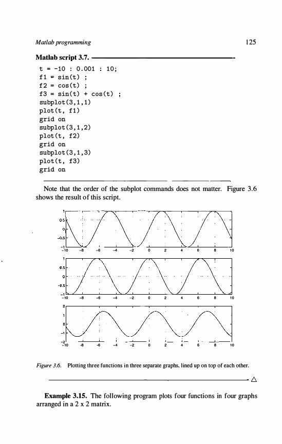
Matlab programming
Matlab script 3.7. -----------------, t = - 10 : 0 . 00 1 f l sin (t ) f 2 = cos (t ) ;
1 0 ;
f3 = sin ( t ) + cos (t ) subplot (3 , 1 , 1 ) plot (t , f l ) grid on subplot (3 , 1 , 2 ) plot (t , f2 ) grid on subplot (3 , 1 , 3) plot (t , f3) grid on
1 25
Note that the order of the subplot commands does not matter. Figure 3 .6 shows the result of this script.
��K�_t��Z�L{l�··J - 10 -8 -6 -4 -2 0 2 4 6 8 1 0
tlt\/::\Z\] -10 -8 -6 -4 -2 0 2 4 6 8 1 0
2 lZ=��j�� -10 -8 -6 -4 -2 0 2 4 6 8 1 0
Figure 3.6. Plotting three functions in three separate graphs, l ined up on top of each other.
--------------------------------------------- 6
Example 3.15. The following program plots four functions in four graphs arranged in a 2 x 2 matrix.

1 26 MATHEMATICS: THE LANGUAGE OF ECE
A note on good practice is in order here. If signals are to be compared using different graphs, the graphs should have the same scaling. Such scaling produces much more easily interpreted results. For example, in Figure 3.6, it would appear at a first glance that the signal in the bottom graph has a smaller amplitude than the other two.
The Matlab command axis is used to enforce common scaling in different plots, as the following script demonstrates. The syntax of the command is
axi s ( [xmin xmax ymin ymax] )
The parametersxmin andxmax determine the minimum and maximum values for the horizontal axis. The parameters ymin and ymax determine the minimum and maximum values for the vertical axis.
Matlab script 3.8. -----------------
% Define the time interval tmin = -3 ; tmax = 3 ; step = 0 . 00 1 ; t = tmin : step : tmax ;
% Define the four funct ions f 1 sin (2*pi*t ) f 2 cos (2*pi*t ) f3 sin (2*pi*t ) + cos (2*pi*t ) f4 sin (2*pi*t ) - cos (2*pi*t )
% Now plot in four separate graphs subplot (2 , 2 , 3) plot (t , f3) xlabel ( ' t ' ) ylabel ( ' f3 (t) ' ) grid on % Force the range f or the time axis to [-3 , 3] % Force the range f or the vertical axis to [-2 , 2] axi s ( [tmin tmax -2 2] )
subplot (2 , 2 , 1 ) plot (t , £ 1 ) xlabel ( ' t ' ) ylabel { ' f 1 (t ) ' ) grid on

Matlab programming 1 27
axis ( [tmin tmax -2 2] )
subplot (2 , 2 , 2) plot (t , f 2 ) axis ( [tmin tmax -2 2] ) xlabel ( , t ' ) ylabel ( ' f2 (t ) , ) grid on
subplot ( 2 , 2 , 4) plot (t , f4) xlabel ( , t ' ) ylabel ( ' f4 (t ) ' ) grid on axis ( [tmin tmax -2 2] )
Figure 3 .7 displays the four signals. Note that setting the (common) limits for the vertical axis may require some "trial and error" effort, if the signals are not as simple as the ones in this example.
-2 '-------------' -3 -2 -1
-2 '---------------' � 4 � 3
Figure 3. 7. Setting common axis scaling in separate plots.
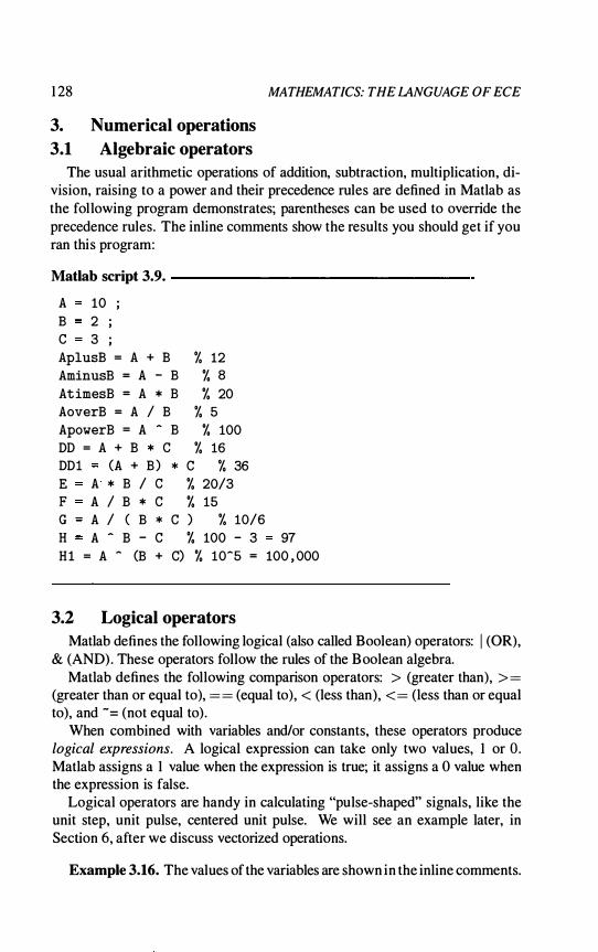
1 28 MATHEMATICS: THE LANGUAGE OF ECE
3. Numerical operations
3.1 Algebraic operators
The usual arithmetic operations of addition, subtraction, multiplication, division, raising to a power and their precedence rules are defined in Matlab as the following program demonstrates; parentheses can be used to override the precedence rules. The inline comments show the results you should get if you ran this program:
Matlab script 3.9. ----------------
A 10 ; B 2 ; C 3 ; AplusB = A + B AminusB = A - B AtimesB = A * B AoverB = A / B ApowerB = A � B DD = A + B * C
% 12 % 8 % 20
% 5 % 100
% 16 DDl (A + B ) E A * B / C
* C % 36 % 20/3
F A / B * C % 15 G A / ( B * C ) % 10/6 H A � B - C % 100 - 3 97 H l = A � (B + C) % 10�5 = 100 , 000
3.2 Logical operators
Matlab defines the following logical (also called Boolean) operators: I (OR), & (AND) . These operators follow the rules of the Boolean algebra.
Matlab defines the following comparison operators: > (greater than), >= (greater than or equal to), == (equal to) , < (less than), <= (less than or equal to), and - = (not equal to) .
When combined with variables and/or constants, these operators produce logical expressions. A logical expression can take only two values, I or O . Matlab assigns a I value when the expression is true; it assigns a 0 value when the expression is false.
Logical operators are handy in calculating "pulse-shaped" signals, like the unit step, unit pulse, centered unit pulse. We will see an example later, in Section 6, after we discuss vectorized operations.
Example 3.16. The values of the variables are shown in the inline comments.
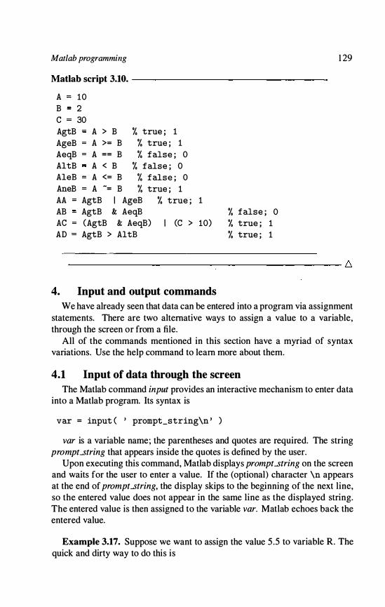
Matlab programming
Matlab script 3.10. ----------------
A 10 B 2 C 30 AgtB A > B % true ; 1 AgeB A >= B % true ; 1 AeqB A == B % f alse ; 0 AltB A < B % f alse ; 0 AleB A <= B % f alse ; 0 AneB A -= B % true ; 1 AA AgtB I AgeB AB AgtB & AeqB AC (AgtB & AeqB) AD AgtB > AltB
% true ;
I (C >
1 % f alse ; 0
10) % true ; 1 % true ; 1
1 29
-------------------------------------------- 6
4. Input and output commands
We have already seen that data can be entered into a program via assignment statements. There are two alternative ways to assign a value to a variable, through the screen or from a file.
All of the commands mentioned in this section have a myriad of syntax variations. Use the help command to learn more about them.
4.1 Input of data through the screen
The Matlab command input provides an interactive mechanism to enter data into a Matlab program. Its syntax is
var = input ( , prompt_string\n ' )
var is a variable name; the parentheses and quotes are required. The string prompt..string that appears inside the quotes is defined by the user.
Upon executing this command, Matlab displays prompt..string on the screen and waits for the user to enter a value. If the (optional) character \n appears at the end of prompt..string, the display skips to the beginning of the next line, so the entered value does not appear in the same line as the displayed string. The entered value is then assigned to the variable var. Matlab echoes back the entered value.
Example 3.17. Suppose we want to assign the value 5 .5 to variable R. The quick and dirty way to do this is

1 30
R = input ( ' R=??\n ' ) 5 . 5
A more polite way might be
MATHEMATICS: THE LANGUAGE OF ECE
R = input ( ' Please enter the value of R : \n ' ) 5 . 5
and the New York variation is
R = input ( ' Gimme da freaking value , OK?\n ' ) 5 . 5
-------------------------------------------,- �
4.2 Output of data to the screen
We have already seen that omitting the ; sign from the end of an assignment statement causes the value of the variable to be displayed.
The Matlab command disp can also be used to display the value of a variable or variables. Its syntax is
disp ( var )
var is the variable's name. The command
disp ( ' string ' )
will display a string on the screen.
Example 3.18. The following script will produce a "neat" output of the variables' values.
MatIab script 3.11. -------------------------------, A 10 ; B 20 ; C A + disp ( ' A disp (A) disp ( ' B disp (B) disp ( ' C= , ) disp (C)
B ; , )
, )
--------------------------------------------,- �
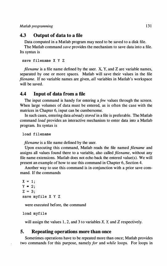
Matlab pmgramming 1 3 1
4.3 Output of data to a file
Data computed in a Matlab program may need to be saved to a disk file. The Matlab command save provides the mechanism to save data into a file.
Its syntax is
save f ilename X Y Z
filename is a file name defined by the user. X, Y, and Z are variable names, separated by one or more spaces. Matlab will save their values in the file filename. If no variable names are given, all variables in Matlab's workspace will be saved.
4.4 Input of data from a file
The input command is handy for entering a few values through the screen. When large volumes of data must be entered, as is often the case with the matrices in Chapter 6, input can be cumbersome.
In such cases, entering data already stored in a file is preferable. The Matlab command load provides an interactive mechanism to enter data into a Matlab program. Its syntax is
load f ilename
filename is a file name defined by the user. Upon executing this command, Matlab reads the file named filename and
assigns all values found there to a variable, also called filename, without any file name extensions. Matlab does not echo back the entered value(s). We will present an example of how to use this command in Chapter 6, Section 4.
Another way to use this command is in conjunction with a prior save command. If the commands
X 1 · , Y 2 ; Z 3 ; save myf ile X Y Z
were executed before, the command
load myf ile
will assign the values 1 , 2 , and 3 to variables X, Y, and Z respectively.
5. Repeating operations more than once
Sometimes operations have to be repeated more than once; Matlab provides two commands for this purpose, namely for and while loops. For loops in
1 32 MATHEMATICS: THE lANGUAGE OF ECE
Matlab are used to repeat operations for a known number of times; while loops are used to repeat operations until a logical condition is false. The syntax of both commands is similar to the one used in C.
5.1 For loops
The structure of afor loop is the following:
f or variable_name = start_value : increment % operations t o be repeated
end
The for and end keywords are required; variableJlame is the name of any variable you choose. start_value, increment, and last-value must be arithmetic expressions. If start_value is greater than last-value, the for loop will not be executed unless the increment is negative.
Example 3.19. The commands
Matlab script 3.12. ----------------
f or abc = 0 : 1 0 30 disp ( abc)
end
will display the numbers 0, 10, 20, and 30.
Example 3.20. Suppose we want to calculate the sum
(3.2)
This sum can be calculated recursively as follows: let An denote the sum of the first n terms in the summation. We can write
Al = ( 1 )2 , A2 = ( 1 )2 + (2)2 , A3 ( 1 )2 + (2)2 + (3)2
and so on and so forth. With this notation, the desired sum is equal to A3Q , and

Matlab programming 1 33
An = An- I + n2 , n = 2 , 3, · · · , 30 . (3. 3)
If we define Al = 1 , we can evaluate equation 3 .3 for n = 2, 3 , . . . , 30. Here is a Matlab program to calculate the sum in equation 3 .2 .
Matlab script 3.13. ----------------
A ( 1 ) = 1 ; % the initi al value for n = 2 : 30
A (n) = A (n- 1 ) + n-2 end disp ( ' The sum i s equal to ' ) disp (A (30) )
5.2 While loops
The structure of a while loop is the following:
while ( condition_is_true ) % operat ions to be repeated
end
Example 3.21. The commands
Matlab script 3.14. -----------------
a = 10 ; whil e ( a > 0 )
i f a < 5 ,
end
a = 0 ; disp ( a)
else a = a - 1 disp (a)
end
will make the while loop execute 7 times; the displayed values of a will be 1 0, 9, 8 , 7, 6, 5, O. ---------------------------------- 6

1 34 MATHEMATICS: THE LANGUAGE OF ECE
6. Vectorized operations
For loops usually take a long time to execute. Vectorizing operations speeds up execution times dramatically.
Consider two variables X and Y that have the same number of elements. Suppose that an arithmetic (or logical) operation must be performed on them, element by element. A typical example of such operations is all the point-wise operations on functions we discussed in Chapter 1 , Section 1 .3 .
For example, consider the signal f(t) = sin( lOt) i n Example 3.2, and let g{t) = cos( lOt ) . Suppose that their product h(t) = f(t)g(t) must be evaluated for all values of t in the time interval [-10, 20] .
With a for loop, the commands to calculate the signal h(t) might be
Matlab script 3.15. ----------------
t - 1 0 : 0 . 00 1 20 ; f sin ( 10*t ) ; g cos ( 10*t ) ; N length (t) ; f or n = 1 : N
h (n) = f (n) * g (n) ; end
In the above script, t is a one-dimensional array with 30,001 elements. The statements f = sine 1 0*t); and g = cos( 10*t); are two simple examples of vectorized operations.
We can vectorize the calculation of the signal h( t) as follows:
Matlab script 3.16. ----------------
t -10 : 0 . 00 1 20 ; f sin ( 10*t ) ; g cos ( 10*t ) ; h = f . * g ;
(N ote the presence of the dot in front of the * operator. ) When applied to two lists of numbers, the . * operator performs the element by element multiplication of the lists. The result is another list with the same number of elements.
Other vectorized operators in Matlab are introduced in the following example.

Matlah programming 1 35
Example 3.22. Consider the commands
Matlab script 3.17. -----------------,
t -10 : 0 . 001 20 ; f sin ( 10*t ) ; % vectorized funct ion call g cos ( 10*t ) ; % vectorized function call
power = 2 ; h1 f . f g % vectorized division h2 = g . -power % vectorized raise to a power
-------------------------------------------- �
Example 3.23. The speedup in vectorized operations can be significant. The Matlab built-in variable clock and function etime can be used to measure the speedup, as the following script demonstrates.
The function clock is the value of the system clock. The statement "to =
clock;" saves the current clock value in variable to. The statement "etime(clock, to)" calculates the difference between the current clock value and the variable to. Therefore, with the placement of the two statements as shown in the script, the elapsed time for the calculation of f (t) / g( t) with the two methods is estimated.
Matlab script 3.18. -----------------
t f g
-10 : 0 . 001 sin ( 10*t ) ; cos ( 10*t ) ;
t o = clock ; power = 2 ; h1 f . f g
20 ;
t 1 = etime (clock , tO) ;
N = length (t ) ; t2 = clock ; f or n = 1 : N
h en) = f en) f g (n) ; end t3 = etime (clock , t2) ;
% start the clock
% vectorized divis i on % end the clock
disp ( ' Elapsed time , vectorized division ' ) disp (t 1 )
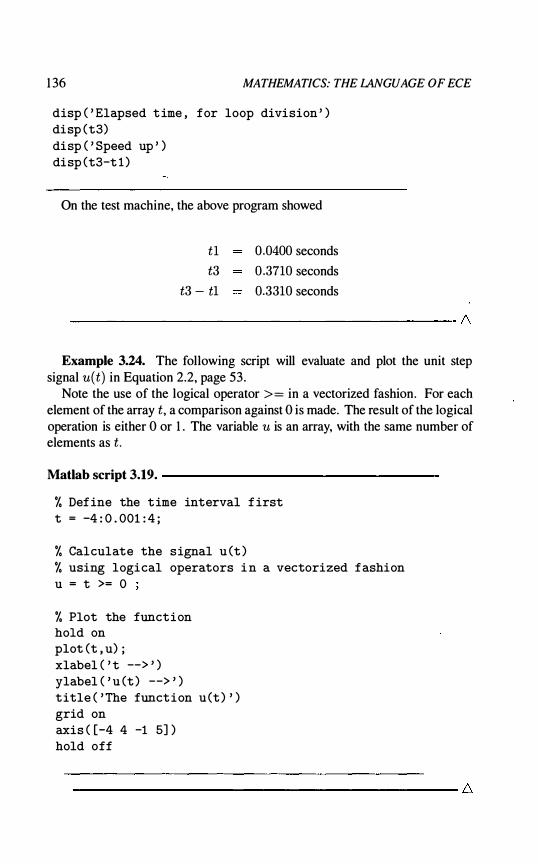
1 36 MATHEMATICS: THE LANGUAGE OF ECE
disp ( ' Elapsed t ime , for loop division ' ) disp (t3) disp ( ' Speed up ' ) disp (t3-t l )
On the test machine, the above program showed
tl t3
t3 - t1
0 .0400 seconds 0 .3710 seconds 0.3310 seconds
------------------------------------------- �
Example 3.24. The following script will evaluate and plot the unit step signal u(t) in Equation 2.2, page 53.
Note the use of the logical operator >= in a vectorized fashion. For each element of the array t, a comparison against 0 is made. The result of the logical operation is either 0 or 1 . The variable u is an array, with the same number of elements as t .
Matlab script 3.19. -----------------
% Def ine the t ime interval f irst t = -4 : 0 . 001 : 4 ;
% Calculate the signal u (t ) % using logical operators i n a vectorized f ashion u = t >= 0
% Plot the function hold on plot (t , u) ; xlabel ( ' t --> ' ) ylabel ( ' u (t ) --> ' ) title ( ' The funct ion u (t ) ' ) grid on axis ( [-4 4 -1 5] ) hold off
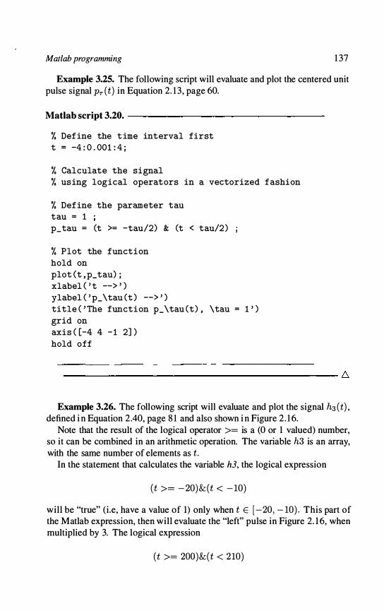
Matlab programming 1 37
Example 3.25. The following script will evaluate and plot the centered unit pulse signal Pr (t) in Equation 2. 1 3 , page 60.
Matlab script 3.20. -----------------
% Def ine the t ime interval first t = -4 : 0 . 001 : 4 ;
% Calculate the signal % using logical operators in a vectorized f ashion
% Def ine the parameter tau tau = 1 p_tau = (t >= -tau/2) & (t < tau/2)
% Plot the function hold on plot (t , p_tau) ; xlabel C ' t --> ' ) ylabel ( ' p_\tau (t ) --> ' ) title ( ' The function p_\tau (t ) , \tau = 1 ' ) grid on axis ( [-4 4 - 1 2] ) hold off
------------------------,· 6
Example 3.26. The following script will evaluate and plot the signal h3 (t) , defined i n Equation 2 .40, page 8 1 and also shown i n Figure 2 . 1 6.
Note that the result of the logical operator >= is a (0 or I valued) number, so it can be combined in an arithmetic operation. The variable h3 is an array, with the same number of elements as t.
In the statement that calculates the variable h3, the logical expression
(t >= -20)&(t < -10)
will be "true" (i .e, have a value of 1) only when t E [-20 , - 10) . This part of the Matlab expression, then will evaluate the "left" pulse in Figure 2. 1 6, when multiplied by 3. The logical expression
(t >= 200)&(t < 210)

1 38 MATHEMATICS: THE LANGUAGE OF ECE
will be "true" (i.e, have a value of 1 ) only when t E [200, 2 10 ) . This part of the Matlab expression, then will evaluate the "right" pulse in Figure 2 . 1 6, when multiplied by 5 .
Matlab script 3.21. -----------------
% Define the t ime interval f irst t = -50 : 0 . 001 : 250 ;
% Calculate the signal h3 (t ) % using logical operators in a vectorized f ashion % and in an arithmetic operation p1 = 3 * ( (t >= -20) & (t < -10) ) p2 = 5 * ( (t >= 200) & (t < 210) ) h3 = p1 + p2 ;
% Plot the function hold on plot (t , h3) ; xlabel ( ' t --> ' ) ylabel ( ' h_3 (t ) --> , ) title ( ' The function h_3 (t ) ' ) grid on axis ( [-50 250 - 1 6] ) hold off
7. Functions
We have already seen some built-in Matlab functions, l ike sin(t) and cos(t). These functions accept an argument and return a value.
We can define our own functions in Matlab (pretty much like we can define procedures in C). The statements
Matlab script 3.22. -----------------,
function y = mysin (x) y = x - x�3 / (1 * 2 * 3) + x�5 / (1 * 2 * 3 * 4 * 5) return
define a function whose name is mysin. The function calculates an approximation to the sine function by using the first three terms of its Taylor series

Matlab programming 1 39
expansion (see Equation 1 .27, page 30 in Section 1 .5 .2) . The keyword function is required. The return statement is not needed but is good practice. Notice that the variable name y that appears in the function declaration also appears inside the body of the function. This is the value that the function cail returns.
Example 3.27. The definition
Matlab script 3.23. -----------------
functi on avg = myaverage (x , y , z) avg = x + y + z avg = avg / 3 return
and the call
aver = myaverage (3 , 1 , 8) disp ( aver)
will produce a value aver = 4. -------------------------------------------- 6
Functions can return more than one value, as the following example demonstrates.
Example 3.28. The statements
Matlab script 3.24. ------------------
funct i on [sine , cosine , tangent] s ine = sin (x) ; cosine = cos (x) tangent = tan (x) ; return
trignumbers (x)
define a function that returns three values, namely the sine, cosine and tangent of the argument x. Note that the brackets in the function declaration are required.
The call
x = pi ; [sinepi , cosinepi , tangentpi] trignumbers (x)
will produce the values sinepi=O, cosinepi=-l . tangentpi=O.
Table 3 . 1 summarizes some of the Matlab built-in functions.

140
Table 3. 1 . Matlab built-in functions.
MATHEMATICS: THE LANGUAGE OF ECE
II Function " Marlab name II sin(t) sin(t)
cos(t) cos(t)
tan(t) tan(t)
sin- 1 (t) asin(t)
cos-1(t) acos(t)
tan-1(t) atan(t)
et exp(t)
loge(t) log(t)
loglO(t) logIO(t)
.;t sqrt(t)
I t I abs(t)
7.1 A library of Matlab functions for signal generation
Certain signals appear very frequently in this and many other courses. It will be useful to create a library of Matlab functions that implement such signals, which you can use for years to come.
Table 3.2 below summarizes some of these signals that Matlab has already implemented as built-in functions. The command help square will give you more details on the available options in calling the periodic pulse (and similarly the other functions) . You can easily build more signals based on them, as we will see in the problem section.
Table 3.2. Matlab built-in signals.
Signal
periodic pulse
periodic ramp
sinc
triangular pulse
rectangular pulse
Matlab name
squa re(t, duty _cycle)
sawtooth( t, width)
sinc(t)
tripuls( t, T) rectpuls( t)
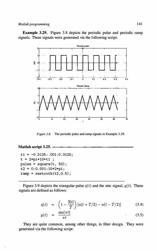
Matlab programming 14 1
Example 3.29. Figure 3 .8 depicts the periodic pulse and periodic ramp signals. These signals were generated via the following script:
Periodic pulse
- r-- ,.....- .r- . r-- -¥i 0
1 ....... ....... ....... '-- ....... ....... . -2 -0.4 -0.3 -0.2 -0. 1 0.1 0.2 0.3 0.4
Periodic Ramp
-2�----�--��--�----�----�----�----� o � � � � ro
Figure 3.8. The periodic pulse and ramp signals in Example 3 .29.
Matlab script 3.25. ----------------
t 1 = -0 . 3 125 : . 001 : 0 . 3125 ; t = 2*pi* 10*t 1 ; pulse = square (t , 50) ; t 2 = 0 : 0 . 00 1 : 10*2*pi ; ramp = sawtooth (t2 , 0 . 5) ;
Figure 3.9 depicts the triangular pulse q(t) and the sinc signal, y(t) . These signals are defined as follows :
q(t)
y(t)
(1 - 2� 1 ) [u(t + T/2) - u(t - T/2 )]
sin( 7ft) 7ft
(3.4)
(3 .5)
They are quite common, among other things, in filter design. They were generated via the following script :

142 MATHEMATICS: THE LANGUAGE OF ECE
Triangular pulse signal, T = 4
1 .5
� 0.5
-0.5
_1 � __ L-__ L-__ L-__ � __ � __ � __ � __ � __ �� -5 -4 -3 -2 -1
Sine signal y(l) = sin(nl)/(nl)
Figure 3.9. The triangular pulse and sine signals in Example 3.29.
Matlab script 3.26. ----------------
t3 = -5 : 0 . 01 : 5 ; T = 4 ; triangularpulse y = sinc (t3) ;
tripuls (t3 , T) ;
----------------------------------------- �
Skillset to be developed
• Write Matlab scripts to produce a "good" plot of a signal, especially a periodic one.
• Write Matlab functions to calculate simple signals.
Connection to other ECE courses
You will use the computer language developed in this chapter primarily in the following ECE courses : 301 , 303 , 402, 420, 421 , 422, 435 , 436, 45 1 , 455 and 456. As a matter of fact, Matlab is much more powerful than what this introductory chapter portrays: in the above mentioned courses, you will be introduced to a plethora of built-in functions that implement concepts such as
Matlab programming 143
convolution of signals, filters, transfer functions, calculation of Laplace and Fourier transforms, and feedback.

144 MATHEMATICS: THE LANGUAGE OF ECE
Problems
Plots of periodic signals
3.1. Consider a CPU with a 500 MHz clock. The clock generator signal Pc( t) (see Figure 2 .9 , page 63) for this CPU has a period ofT = 2 nanoseconds. Write a MatIab program to evaluate and plot the signal over the interval [-lOT, 10Tj . Within a period, you must display exactly 1 00 points. You must label both axes.
3.2. Consider a periodic signal, one period of which is shown in Figure 9.4, page 454. Write a Matlab program to evaluate and plot the signal over 4 periods.
3.3. Consider the "periodic ramp" signal , an example of which is shown in Figure 9.9, page 465 . Write a Matlab program to reproduce the plot in Figure 9.9.
3.4. Write a Matlab program to evaluate and plot the signals
VI (t) sin(27rt) V2 (t) cos(27rt) V3 (t) sin(27rt) + cos(27rt) V4 (t) sin(27rt) cos(27rt)
(3.6)
for t E [-4, 4j . How many periods does the graph cover? You may use a common graph for all 4 plots, if you like.
3.5. Let T be the period of the signal v(t) defined in Equation 3 .7 :
v(t) = 3 cos(27r200t + 7r/3 ) . (3 .7)
Write a Matlab program to evaluate and plot the signal over the interval [-T, 3Tj . Within a period, you must display exactly 1 00 points. You must label both axes.
3.6. The following Matlab program plots the function
v (t ) = 3 cos(27r200t) + 2 sin(27r400t + 7r/2)
t = 0 : step : Tmax ; v = 3 * cos (2*pi*200*t) + 2 * sin (2*pi*400*t + pi/2) ; plot (t , v) xlabel ( ' time ( seconds ) ' ) ylabel ( ' signal v et ) ' )
Matlab programming 1 45
What is the period of the signal v(t) ? Suppose that we want to produce a plot that covers exactly 4 periods and has exactly 20 samples per period. Determine the appropriate values of the step and Tmax variables.
3.7. Consider -Example 2. 1 7 , and in particular the sum signal in Equation 2.36, page 76. Let F2 = 2Fl = 60. Plot the three signals
Verify by inspection the results of that example.
*3.8. This problem deals with generation of "nice" Matlab plots.
Write a Matlab function nice..sine-plot(A, F, theta, k), that will plot the signal s (t) = A sin(21TFt + theta) for k periods. The plot should show time values that are both positive and negative. The function should adjust the discretization parameter so that the plot "looks nice" irrespective of the choice of the parameter F.
2 Can you determine the mathematical relationship between the discretization step and the frequency parameter?
Arithmetic operations and operations on signals
3.9. Let t = 0 : 0.05 : 1 . Use vectorized commands (i .e . , no for loops) to compute the value of the functions (a) v 1 (t) = COS(21T0.Olt + 1T/3) (b) v2(t) = lOe-2t (c) v3(t) = v1 (t) . v2(t)
3.10. Consider the signal s(t) = 50 COS(21T60t + 1T /3) . Let 0 ::; t ::; 10 seconds. Use both a for loop and a vectorized command to calculate s (t) over the given interval , with a resolution of 1 J-Lsec. Calculate how much slower the for loop is, using the etime command.
3.11. Write a Matlab script to calculate and plot the unit pulse signal p(t) , in Equation 2. 1 2 , page 59, for t E [-20, 20] using vectorized commands and logical operators. Choose to = 3.
3.12. Write a Matlab script to calculate and plot the centered unit pulse signal PT(t ) , in Equation 2 . 1 3 , page 60, for t E [-20, 20] using vectorized commands and logical operators. Choose T = 5 .
1 46 MATHEMATICS: THE LANGUAGE OF ECE
3.13. Write a Matlab script to calculate and plot the signal 81 (t) in Problem 2.35 . Choose T = 2.
3.14. Write a Matlab script to calculate and plot the signal 82 (t) in Problem 2.36. Choose T = 1 . 3.15. Write a Matlab script to calculate and plot ilie signal 83 (t) in Problem
2.37. Choose T = 4.
3.16. Write a Matlab script to calculate and plot ilie signals 84 (t) through 89 (t) in Problem 2.38.
*3.17. In the Matlab command window, type load handel; this will load ilie first five Hallelujah's from Handel 's Messiah, in a vector named y. This vector is your signal 8 ( t) .
1 Plot the vector y, using a plot(y) command. Play the sound using the sound(y) command. Play it again.
2 The sound was sampled, digitized and stored in Matlab wiili a sampling frequency of 8 1 92 Hz. This means iliat the time difference between two samples is 1/8192 � 0. 122 milliseconds. Using the length(y) command, you can see that ilie vector y has 73 , 1 1 3 elements. Therefore, the Matlab variables y( l ) , y(2) and y(3) store the signal values 8(0) , 8(0. 122) and 8(0 .244) respectively. Find out how long the sound is, in seconds; in other words, find what y(731 13) stores.
3 Plot the vector y versus time, using a plot(t, y) command. You will have to create the time vector t. The minimum and maximum values of t define the domain, DB , over which the signal 8 (t) is defined. What are these values?
4 Create, in Matlab, a new signal f(t) = 8( -t) . Plot and play f(t) .
5 Create, in Matlab, a new signal f(t) = 8(t - to) . u(t - to) , where u(t) is the unit step signal . Plot and play f(t) . Use to values of 1 , 2, and 5 seconds. What domain have you used for f(t)? Is it ilie same as DB? If not, justify your selection.
6 Create, in Matlab, a new signal f(t) = 8(at) . Plot and play f(t) . Use a values of 2, 3 , and 4. What domain have you used for f(t) ? Is it the same as DB? If not, justify your selection.
Matlab programming 1 47
Writing and using functions
3.18. For safety reasons, electrical devices l imit the output voltage Vout (t ) to a maximum al lowed value A, regardless of the value of the i nput voltage Vin ( t ) . Mathematically, we can represent such devices via the function Vout (t ) = f(Vin ( t ) ) , where { V,
f(v) = A, -A.
-A :::; v :::; A, v > A, v < -A.
(a) Write a function clip(v,A) to simulate th is device. (b) Write a script that calls this function with a sinusoidal input voltage
V'in(t) = 10 cos(2nt) . Use A = 2. Plot both the input and output on the same graph, for t E [-5, 5] .
(c) Repeat part (b) for the i nput voltage Vin (t ) = lOt .
. 9 A ful l-wave rect ifier is an electrical device that implements the operation described by the fol lowing function. The signals Voul (t) and Vin ( t) represent the output and i nput voltages respectively.
if Vin (t ) 2: 0, i f Vin (t ) < O.
An al ternative, more compact notation would be Vout .(t ) = I Vin (t ) l . (a) Write a [unction fivJect!fier(v) to simulate the recti fier device. (b) Write a script that cal l s this function with a s inusoidal i nput voltage
Vin (t) = 2 cos(2nt) . Plot both the input and output on the same graph, for t E [-5, 5] .
(c) Repeat part (b) for the i nput vol tage Vin (t ) = lOt.
3.20. A hal f-wave rect ifier is an electrical device that implements the operation described by the fol l owing function. The signals Vou t (t) and Vin (t ) represent the output and input voltages respectively.
if Vin (t ) 2: 0, if Vin (t ) < 0,
An alternative, compact notation would be Vout (t ) = max(O, Vin (t ) ) . (a) Write a function hWJect!fier(v) to simulate this rect ifier device. (b) Write a script that cal l s this function with a sinusoidal i nput voltage
Vin (t ) = 2 cos(2nt) . Plot both the input and output on the same graph, for t E [-5 , 5] .
(c) Repeat part (b) for the input vol tage Vin (t ) = lOt.
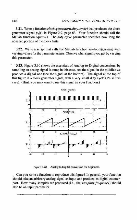
1 48 MATHEMATICS: THE LANGUAGE OF ECE
3.21. Write a function clock_generator(t,duty_cycle) that produces the clock generator signal Pc(t) in Figure 2.9, page 63. Your function should call the Matlab function squareO. The duty_cycle parameter specifies how long the nonzero portion of the clock lasts.
3.22. Write a script that calls the Matlab function sawtooth(t, width) with varying values for the parameter width. Observe what signals you get by varying this parameter.
3.23. Figure 3 . l O shows the essentials of Analog-to-Digital conversion: by sampling an analog signal (a ramp in this case, see the signal in the middle) we produce a digital one (see the signal at the bottom). The signal at the top of this figure is a clock generator signal , with a very small duty cycle ( 1 % in this case) . (Hint: you may want to use this signal in your function.)
Periodic pulse train
· J 111111111111111 i II II II I I II" 1111 I I I !HI II II II i IIII' 1 -15 -10 -5 0 10 1 5
· J J(l;4/?L± 1 -15 -10 -5 0 5 10 1 5
� :� . . . , ••. . , d i l l · 1·. :;l-"�"' I I I ,· .. , 1 1 11 . . · ·. · · 1 '<:' 11111 I I II 1111 ' II III' .
-1 . . . . . . . •
�L-____ L-____ � ____ � ____ � ____ � ____ � -15 -10 -5 5 10 15
Figure 3. 10. Analog to Digital conversion for beginners.
Can you write a function to reproduce this figure? In general, your function should take an arbitrary analog signal as input and produce its digital counterpart. How many samples are produced (i.e. , the sampling frequency) should also be an input parameter.

Matlab programming 149
Using Matlab to explore mathematical questions
*3.24. Suppose you have two sinusoidal signals
and S2 (t) = A2 sin(27rF2t + 02 )
with frequency parameters FI and F2, that are integers, but not necessarily equal.
The period of the generic function sin(y) is 27r (i .e . , sin(y + 27r) = sin(y) . What is the period of SI (t) ? Answer this through a Matlab plot of SI (t) , in which you set specific values for the parameters AI , FI and 01 .
2 Does the period of S I (t) depend on the parameter AI? Answer this by plotting S I (t) (on the same graph, using the hold on command) for a few values of Al first2 , say, Al = -1 , +1 , - 10 , +10. Then prove your conjecture mathematically.
3 Does the period of SI (t) depend on the parameter OI ? Answer this by plotting SI (t) (on the same graph, using the hold on command) for a few values of 01 first, say, 01 = - 10, + 1 , - 1000 , +100. Then prove your conjecture mathematically.
4 Does the period of SI (t) depend on the parameter FI ? Answer this by plotting SI (t) for a few values of FI first, say, FI = +1 , +2 , +3. Then prove your conjecture mathematically.
5 What is the period of the signal s(t) = Sl (t) + S2 (t )? Answer this by plotting s(t) first. Then prove your finding mathematically.
6 What is the period of the signal s(t) = 5S1 (t) - 3S2 (t) ? Answer this by plotting s ( t) first. Then prove your finding mathematically, by generalizing to a signal
where Q and f3 are real numbers.
7 Suppose you have one more sinusoidal signal
2This is one example of the "engineering" proof methodology. You know. of the sort, "I is a prime number. 2 is a prime number. 3 is a prime number. therefore all positive integers are prime numbers."

1 50 MATHEMATICS: THE LANGUAGE OF ECE
What is the period of the signal s(t) = SI (t) + S2 (t) + S3 (t) ? Answer this by plotting s(t) first. Then prove your finding mathematically. If you played enough with signals now, you should be able to both formulate and prove a mathematical theorem of the form: (Put your name here) Theorem: Let k be any positive integer. Let
be sinusoidal functions with arbitrary amplitudes Ak, frequencies Fk and phases Ok . The period T of the "sum" sinusoidal function
put the appropriate formula here
IS put the appropriate formula here
*3.25. Consider the cell phone signals in example 2. 1 9.
1 Let SI (t) denote the signal that the base station antenna receives. Write an expression that expresses SI (t) as a function of s( t) , dA , the reflected signal Sr (t) , the speed of light and the length dB of the reflection path.
2 Suppose for simplicity that
s(t) = 3 sin(27rFt) ,
where F = 1000 Hz (an audible tone). Let
dA = 1 , 000 meters, dB = 1 , 010 meters .
For the purposes of these discussions, you may assume that the speed oflight is 300,000,000 meters/sec. Accurately plot (using subplot) the following signals :
• s( t) at the cell phone
• s( t) at the base station
• the reflected signal at the base station
• SI (t) at the base station
3 Use the Matlab sound command to play s(t) and S I (t) . Do you "hear" any difference? In other words, did reflection cause any trouble?

Matlah programming 1 5 1
4 Consider a more realistic signal now. In the Matlab command window, type load handel; this will load the first five Hallelujah's from Handel 's Messiah (sorry, no Metallica sounds in Matlab yet) . Suppose that this is your signal s(t) now. Repeat the previous question. Increase the value of dB until you "hear" a difference.
Challenge problem 3.1. Putting many concepts and skills together, or an engineering look at some trigonometric theory
Applying the Taylor series formula to approximate the value of a function f(t) at some point t = to can give very large errors. A closer look at the terms of the Taylor series should explain that behavior: terms l ike x2 , x3 , x4 , etc . grow extremely fast when x > 1 and go to 0 extremely fast when x < l .
Taking more and more terms in the approximation (i .e. , using larger values of N) is problematic, since calculation of k! terms for large k is no piece of cake either. (Matlab itself admits that for k > 21 the computation of k! is inaccurate.) Another problem is the following. In an expression like:
f or k = l : N a (k+l ) = x-k/prod ( l : k) ;
. end %prod ( l : k) calculates k !
the values for a(k + 1 ) are computed in the following order:
1 xk is calculated first. If x is large, this computation may be inaccurate.
2 prodO :k) is calculated next. For k > 21 this is definitely inaccurate.
3 the division is performed. Since the terms of the division are inaccurate, the result of the division will be inaccurate.
An approximation that has a chance to be more accurate, therefore, cannot rely on using large values of N. The only viable approach (unless we start thinking outside the box) is to evaluate the sine function at points close to O. With this approach, the issue of dividing two large, inaccurate numbers should have a lesser impact. (Still , it would be nice to avoid such a division . )
The problem then can be stated as follows: Given any value of x, instead of evaluating sin(x) directly, transform x to a value y that's closer to 0, evaluate sin(y) and figure out a way to "relate" sin(y) to sin(x) , that does not involve horrible Taylor series terms.
Here are a few ideas, that draw from trigonometric identities . As a matter of fact, it would be very good practice to look at all trig identities you know and ask the question: how could I use this identity to reduce the computation errors?)
1 52 MATHEMATICS: THE LANGUAGE OF ECE
Idea I. Since for any value of y and any value of the integer k, we have that
sin(y + 2krr) = sin(y) , (3 .8)
we can reduce a "large" x to a number y in the range [0, 2rr) , by dividing x by 2rr and considering the remainder of this division. In other words, if we write
x = 2krr + y, (3.9)
we have sin(x) = sin(2krr + y) = sin(y) .
The intuition and hope is that the transformation in Equation 3 .9 alone should reduce the errors dramatically.
Write a Matlab function my...sinl(x, N) that uses the transformation in Equation 3 .9 before it applies the Taylor series approximation. N is the number of Taylor series terms used in the approximation.
2 Calculate sin(x) for x in the range -lOOrr to lOOrr, three ways: a) using Matlab's built-in function, b) using my...sinl(x,N), and c) using the original value of x in the Taylor series ("brute force"). Use subplot to plot all three graphs.
3 Calculate the errors between (a) and (b) and between (a) and (c), for the same range of x. Use subplot to plot the two error graphs. Are the errors reduced dramatically?
With this transformation, y can still be "large" (i .e. , larger than 1). How can we reduce it to a number smaller than 1 , so that terms like y2 , y3 etc. do not grow up fast? Since rr /6 � 0.5, ideally our goal should be to bring the range down to [0, rr /6) .
Idea 2. Towards this goal , how can you take advantage of the trig identities
sin(rr + z) = - sin(z) = sin( -z)? (3. 1 0)
Given a value of y in the range [0, 2rr), write the relationship between z and y that's the analog of Equation 3 .9. Using this relationship would reduce the range of (the original) x to what values?
Can you write all the trig identities that relate the sine of an angle in the 2nd, 3rd, and 4th quadrant to the sine of an angle in the first quadrant? If yes, in the improved approach you have only to worry about values of the argument in the range [0, rr /2) . And rr /2 � 1 . 5, so errors should be much, much smaller.
1 Write a transformation of the form:

Matlab programming 1 53
w = g(x) (3 . 1 1 )
that guarantees that w E [0, n /2) , for any given value of x.
2 Write a Matlab function my..sin2(x, N) that uses the transfonnation in Equation 3 . 1 1 before it applies the Taylor series approximation . N is the number of Taylor series tenns used in the approximation.
3 Calculate sin(x) for x in the range -lOOn to lOOn, four ways: a) using Matlab's built-in function, b) using my..sinl (x,N), c) using my..sin2(x,N), and d) using the "brute force" approach. Use subplot to plot all four graphs.
4 Calculate the errors between (a) and (b) , (a) and (c) and between (a) and (d), for the same range of x. Use subplot to plot the three error graphs. Are the errors redtJced dramatically when you use my..sin2(x,N)?
Idea 3. n /2, though, is still over 1 . Eventually, what trig identity (or identities) can you take advantage of, to bring the range down to [0, n /6) ?
Write a transfonnation of the fonn:
w = f (x ) (3. 1 2)
that guarantees that w E [0, n /6) , for any given value of x.
2 Write a Matlab function my..sin3(x, N) that uses the transfonnation in Equation 3 . 1 2 before it applies the Taylor series approximation. N is the number of Taylor series tenns used in the approximation.
3 Calculate sin( x ) for x in the range - lOOn to lOOn, two ways: a) using Matlab's built-in function, b) using my..sin3(x,N). Use plot to plot the two graphs.
4 Calculate and plot the errors. Are the errors reduced dramatically when you use my..sin3(x,N)?
What if? The mathematical relationship between the value of an angle () in degree and radian units is
180 ()deg1'ees = ()radians- ' n
What is more advantageous as far as reducing computational errors : to work with x's expressed in radians or degrees? (This is one instance of the concept of time scaling, which we discussed in Chapter 2, applied in a different fashion.)

1 54 MATHEMATICS: THE lANGUAGE OF ECE
How can you use the following trig identities to reduce the errors?
sin(x) = 2 sin (�) cos (�) 1 - cos(x) = 2 sin2 (�)
Write a Matlab program to evaluate your answer, or use your idea as part of the transformation in Equation 3. 1 1 .
What if? How can you modify your programs to avoid the problem we mentioned in calculating a(k + I ) ? Hint: Rewrite
Xk x x x x k!
= 1 · 2" · 3 · · · k and focus on the dots.
Challenge problem 3.2. What the #@ %&! is going on? Or, you be the judge.
On Thursday, September 1 2, 2002, a fellow student mailed me this Matlab program:
Matlab script 3.27. -----------------
clear , clf T = 1 ; f -200 : 1 : 200 ; % frequency range
% Xl : The TA ' s solution to the homework 2 , problem 4 , % the nasty integral . % X2 : my solution . They are the same , % except for one + sign . % However , as this Matlab program proves , % the difference i s small , % always in the order of 10� (-19) ! ! ! % I believe I deserve full credit ; % after all , we are engineers . % I even wrote this Matlab program % to prove my claim .
Xl = T . / (j *pi*2*pi*f ) . * (sin(2*pi*f *T) . / (2*pi*f *T) - cos (2*pi*f*T) ) ;
X2 = T . / (j *pi *2*pi*f ) . * (sin(2*pi*f*T) . /

Matlab programming 1 55
X1_mag=abs (X1 ) ; X2_mag=abs (X2 ) ; Diff = X 1_mag - X2_mag ;
f igure ( 1 ) plot ( f , X1_mag , ' r ' ) ; hold on plot (f , X2_mag , ' b ' ) ; xlabel C ' F ' ) ; ylabel ( ' magnitude ' ) ; grid on ; hold off
f igure (2) plot (f , Diff ) xlabel C ' F ' ) ; ylabel ( ' difference ' ) ; grid on ;
If you run the Matlab program, you will see that the errors are indeed in the 10- 19 range. The student is not lying. If you were in my shoes, would you give the student full credit? Actually, extra credit for writing this Matlab program?
Challenge problem 3.3. Do it if you can. Or, graphical approximations Consider a periodic voltage signal v (t ) with period T = 1 second. The
signal is equal to 1 Volt for the first half of the period and equal to - 1 Volt for the second half. Mathematically, the signal values for t E [0, 1 ) can be expressed as:
v(t) = { I , 0 � t < 0.5 -1 , 0 .5 � t < 1 . (3 . 1 3)
Your friend studies at UnNamed Campus (aka UNC). Students there have at their disposal only one sinusoidal voltage generator, that produces a signal 81 (t) . The generator is good enough to have an amplitude control knob, frequency control knob and phase control knob, since UNC upgraded its equipment in 2001 (after a large donation from an anonymous alumna). Mathematically,
81 (t) = A cos(271-Ft + 0) , (3 . 1 4)
where A, F and 0 are adjustable.

1 56 MATHEMATICS: THE lANGUAGE OF ECE
Write a Matlab program to approximate v(t) with Sl (t) . Plot both signals on the same graph. Play with A, F and () and choose a combination that you feel is the "best". Define what best means to you.
A second donation by an athlete alumnus buys a second sinusoidal voltage generator with the same capabilities. Let's call its output a signal S2 (t) . Write a Matlab program to approximate v(t) with the summation s(t) = Sl (t) + S2 (t) . Plot v(t) and s(t) on the same graph. Play with the A, F and () parameters of both generators and choose a combination that you feel is the "best". You should be able to get a "better" approximation than with one generator.
Repeat for an additional donation (Le. , approximate v(t) with the summation s(t) = S l (t) + S2 (t) + S3 (t».
Now run the file sindrill.m from the course locker. Observe how close to the pulse we can get with 1 , 2, and 3 sinusoids, if the A, F and () parameters are adjusted the way our theory of Fourier series will dictate. Compare the accuracy of the approximations to what you were able to get on your own. If you came up close, you have a darn good engineering intuition ! !
Challenge problem 3.4. Do it if you can. Study the script modulated..signals.m (you will find it in the course locker) .
The signals s l , s4 defined in there must be periodic. What are their periods? Can you tell from the plot in figure 1 if the signal s5 is periodic? In figure 2? In figure 6? Can you prove mathematically what the period of s5 is, if you think the signal s5 is periodic?
Problems you will see in other courses Similar to Chapter 2, this set of problems is intended to highlight the connec
tion of the material in this chapter to other ECE courses. We revisit some problems from Chapter 2; the main emphasis now is to apply the Matlab language to produce accurate plots of realistic signals used in a variety of applications (and even industrial standards). Most of the problems in this section are (slightly) more difficult than the rest of the problems in this chapter. The purpose of putting them here is, one more time, to show you that the (computer) language we have just introduced is tightly connected to realistic ECE applications and other ECE courses (even past ones, like ECE200).
*3.26. (ECE200) Operational amplifiers. The transfer characteristic of an amplifier is shown in Figure 3 . 1 1 .
1 Is this amplifier inverting or non-inverting?
2 What is the gain of the amplifier?

Matlab programming
The transfer characteristic 10.----.r---�-----.----_r----_.----._--__.
��--�----�----�-----L----�----�--� -0.2 -0.1 0.1 0.2 0.3 0.4 0.5
Figure 3. 1 1. The transfer characteristic of the amplifier in Problem 3.26.
3 The input signal is
Vin (t) = 0.05 cos(27rl000t)u(t) .
1 57
Write an equation for the output signal . Plot the input and output signals on the same graph.
4 Is there a DC value in the output signal?
5 The input signal is
Vin (t) = 0.05 cos(27rl000t)u(t) + 0 . 1 cos(27r2000t)u(t) .
Write an equation for the output signal . Plot the input and output signals on the same graph.
6 The input signal is
Vin (t) = 5 cos(27r1000t)u( t ) .
Write an equation for the output signal . Plot the input and output signals on the same graph.
7 Write a Matlab function

1 5 8 MATHEMATICS: THE LANGUAGE OF ECE
vout = arnpliJier (type, gain, devalue , powersupply, vin)
to calculate the output signal vout of a generic amplifier. The input parameters are the following. type, an integer-valued parameter, describes the inverting/non-inverting property of the amplifier. You may use the value 1 to represent a non-inverting amplifier and - 1 for an inverting one. gain, a positive, integer-valued parameter, is the gain of the amplifier. devalue, an integer-valued parameter, is the DC offset of the amplifier. powersupply, a positive, integer-valued parameter, is the (dual) power supply of the amplifier. This parameter will determine the clipping characteristics of the amplifier. vin, a real-valued row vector, is the array that contains the values of the input signal . The function should return an array that contains the values of the output signal . This array should be a real-valued row vector, the same type and dimensionality as vin. Typical calls to and usage of this function would be
% Input signal t = ° : 0 . 001 : 1 ; yin = 0 . 05 * sin (2*pi *60 * t ) ;
type = 1 ; gain = 30 ; devalue = 3 powersupply
% non-inverting amplif ier
% DC off set 9 ; % Dual supply + and - 9 Volts
vout 1 = amplifier (type , gain , devalue , powersupply , yin) plot (t , vin , t , vout 1 )
vout2 = amplifier ( - l , 50 , 0 , 12 , Yin) plot (t , vin , t , vout2 )
vout3 = amplifier (-l , 50 , 0 , 12 , 10 * Yin) plot (t , vin , t , vout3)
8 Would any of the three calls to amplifier in the above script result in clipping? If not, can you change the input parameters to observe such clipping?
*3.27. (ECE200) Operational amplifiers. Write a Matlab function
pi oLarnpliJier (type , gain, devalue, powersupply, vin)

Matlab programming 1 59
to plot the transfer characteristic of an amplifier (i .e . , reproduce a graph similar to the one shown in Figure 3 . 1 1 ) . The input parameters are the same as described in the previous problem.
*3.28. (ECE301) The concept of convolution. Consider Problem 2.42. The goal of this problem is to evaluate and plot the output y(t) in Equation 2.49, page 97. We will use Matlab functions to represent the input signal x( t) and the impulse response signal h(t ) .
Write a Matlab function xinput(t) to calculate the input signal in Equation 2.5 1 . The input argument t is, in general, a row vector. The function should return a vector of the same dimensionality.
2 Write a Matlab function impulseJesponse(t) to calculate the impulse response signal in Equation 2.52. The input argument t is, in general, a row vector. The function should return a vector of the same dimensionality.
3 Write a Matlab function mult(x, h) to calculate the (element-wise) product of two row vectors x and h.
4 The most intuitive, straightforward way to evaluate the output y(t) in Equation 2.49 is to write a for loop, similar to that of the following example. In this script, the Matlab built-in function quad( @f, low, high) calculates the integral
(high f(x)dx
}low
The quad function assumes that the function f(x) is defined in a separate .m file, calledfm.
%% Output evaluation % % Def ine a time interval % over whi ch we ' ll calculate the output t o : 0 . 01 : 5 ; N = l ength (t) ;
% def ine the interval over which % we ' ll calculate the integral t au_min = -20 ; tau_max = 20 dt = 0 . 0 1 ; tau_interval tau_min dt tau_max

1 60 MATHEMATICS: THE LANGUAGE OF ECE
x = xinput (tau_interval ) ; % calculate the input signal
for k = 1 : N tt = t (k) J tau_shift ed_interval = tt - tau_interval ; % calculate the impulse response h = impulse_response (tau_shif ted_interval ) % Now cal culate the integral itself % quad calls the function mult yy = quad (@mult , tau_min , tau_max) ; y (k) = yy ; % store the value in the output array
end
Run this script and plot the output y(t) . If you did everything right, your plot should look like the one in Figure 3 . 1 2.
Convolution integral
2.5
1 .5
� 1 . . . . . . . . . . .
0.5
-0.5
_1 � __ L-__ L-__ L-__ L-__ L-__ L-__ L-__ � __ �� -2 -1 o
Figure 3. 12. The output y(t} in Problem 3.28.
7
5 Calculate the output when the impulse response is the signal in Equation 2.50, page 97. Plot the output.
6 Calculate numerically the output of the RC circuit in Figure 7 � 1 , in page 33 1 , Chapter 7. Verify by comparing the output of your Matlab program to Equation 2 .53 , page 98.

Matlab programming 1 6 1
7 Matlab can save you some of the trouble in evaluating the convolution integral . The built-in function conv(x,h) calculates the integral in Equation 2 .49, page 97, directly. The input argument x must be a vector that defines the input signal x(t) ; the input argument h must be a vector that defines the impulse response signal h(t) . Write a Matlab script that uses the function conv to evaluate the output of the RC circuit in Figure 7. 1 . Note that you have to keep track of the time indices yourself.
*3.29. (ECE303) Signals travelling on transmission lines. Consider Problem 2 .43 .
Write a Matlab function line_voltage(lengthL, vp, gammaL, T, trange, M) to calculate the voltage V(t, x) on a transmission line. The input parameters are: lengthL, a positive, real-valued number, that denotes the length of the line; vp, a positive, real-valued number, that denotes the propagation velocity; gammaL, a positive, real-valued number, that denotes the reflection coefficient; T, a positive, real-valued number, that denotes the duration of the source pulse signal ; trange is the time interval of interest.
Suppose that the number of elements in trange is N. The function should return an N x (M + 1) array that contains the calculated voltage in the following arrangement. The length of the line, d, is partitioned into M intervals, according to the Matlab statements
% discretize the line length into M+ l point s step = d / M x = 0 : step : d
Then the i-th row contains the M + 1 values
V(trange(i) , O · step) , V(trange(i) , l · step) , V(trange(i) , 2 · step) , . . . , V(trange(i) , d) .
2 Use this function in a MatIab script to plot V(t , x) . The input voltage i s a 1 0 nsec pulse, the propagation velocity is given by Equation 2 .54, page 99, the line is 10 meters long, and the reflection coefficient is 0. 1 .
· 3 Use this function in a MatIab script to study the effect of the r L coefficient in Equation 2.56, page 99, on V(t , x) .

1 62 MATHEMATICS; THE LANGUAGE OF ECE
3.30. (ECE305) Transmission lines and three-phase AC voltages. Consider problem 2.44. The goal of this problem is to understand the three phase voltages a bit deeper, with the aid of accurate plots.
1 Plot the three wavefonns in Equations 2.57, 2.58 and 2.59, page 1 0 1 , on the same graph, to see how they relate to each other. Use the rules that we presented in Section 2. 1 to produce a nice plot. If you plot "just a few seconds' worth" of the signals, you may get unintelligible plots, like the one in Figure 3 .4, page 1 23.
2 Plot exactly 5 periods of the three wavefonns on the same graph. Verify from this graph that the maximum voltage of phase b comes after (lags, in ECE305 jargon) that of phase a.
3 Detennine, from the graph, how many seconds after. Then, figure out this lag, analytically, by rewriting Equation 2.58 in the fonn
vw (t) = J2v cos(27r60(t - to) ) .
4 Detennine analytically and from the graph how many seconds phase c lags phase a.
5 Plot exactly 4 periods of the sum
V (t) = vaal (t) + vw (t) + vee/ (t) (3. 1 5)
6 Using trig identities from Chapter 1 , prove that the graph you get from plotting Equation 3 . 1 5 is no mistake. This equation fonns the basis for understanding Delta connections, a basic circuit configuration in ECE305 .
7 Plot exactly 6 periods of the signals
Vaal (t) - vw (t) vaal (t) - vec' (t) Vee' (t) - Vw (t)
(3. 1 6) (3. 1 7) (3. 1 8)
Such equations fonn the basis for understanding Wye connections, another basic circuit configuration in ECE305 .
We will revisit this problem in Chapter4, where we will use complex numbers (phasors) to represent Equations 2.57 to 2.59.

Matlah programming 1 63
*3.31. (ECE402) Touch-tone phones. Consider Problem 2 .45 .
1 Write a Matlab function touchtone( digit) to generate the 50 msec signal that touch-tone phones use to dial numbers. The input argument digit represents a number between 0-9; if this argument takes the values 1 0 or 1 1 , the function should return the dual tones for * and # respectively.
2 Use this function in a script that generates the dual tones for all digits. In the script, use the built-in function sound to hear these tones. Verify this way that your program accurately simulates a touch-tone phone.
3 Run the Matlab demo phone. This demo will bring up a GUI, similar to the one shown in Figure 2.23, page 103 . Check the sound box, so you can hear sounds. (Once again, ignore the power spectrum graph.) Verify, playing with this GUI, that your script runs correctly.
4 Simulate the busy tone signal . How would you program the interruptions?
*3.32. (ECE402) Line codes. Consider Problem 2.46.
Write a Matlab function UNRZ( symbol, bandwidth) to implement the UNRZ l ine code. The input argument symbol represents an ASCII character (see Table 2.2, page 104); the input argument bandwidth represents the rate of the communication line in Mbps. The output is a row vector that stores the waveform.
2 Use this function in a script that generates the UNRZ waveform for the message "Hi Mom, send money", over a 1 0 Mbps line. Plot the waveform, if possible. (If not, what is the problem? How would you modify the requirements in this question, to generate a plot?)
3 Repeat for the PNRZ code.
4 Repeat for the BRZ code.
*3.33. (ECE402) On-Off Keying (OOK). Consider Problem 2.47.
Write a Matlab program to generate both plots in Figure 2.25, page 1 07 .
2 Write a Matlab function ook(symbol, fe, bandwidth) to implement the OOK line code. The input argument symbol represents an ASCII character (see Table 2.2, page 104); the input argumentfc represents the carrier frequency in Mhz; the input argument bandwidth represents the rate of the communication line in Mbps. The output is a row vector that stores the waveform.

1 64 MATHEMATICS: THE LANGUAGE OF ECE
3 Use this function in a script that generates the OOK waveform for the message "Hi Mom, send money", over a 10 Mbps line. Use fe = 100 Mhz. Plot the waveform, if possible. (If not, what is the problem? How would you modify the requirements in this question, to generate a plot?)
*3.34. (ECE402) Binary Phase Shift Keying (BPSK). Consider Problem 2.48.
Write a Matlab program to generate both plots in Figure 2.26, page 1 08 .
2 Write a Matlab function bpsk(symbol, fe, bandwidth) to implement the BPSK line code. The input argument symbol represents an ASCII character (see Table 2.2, page 1 04) ; the input argumentfc represents the carrier frequency in Mhz; the input argument bandwidth represents the rate of the communication line in Mbps. The output is a row vector that stores the waveform.
3 Use this function in a script that generates the BPSK waveform for the message "Hi Mom, send money", over a 1 0 Mbps line. Use fe = 100 Mhz. Plot the waveform, if possible. (If not, what is the problem? How would you modify the requirements in this question, to generate a plot?)
*3.35. (ECE402) Frequency Shift Keying (FSK). Consider Problem 2.49.
Write a Matlab program to generate both plots in Figure 2.27, page 1 07.
2 Write a Matlab function fsk( symbol, f1, jD, bandwidth) to implement the FSK line code. The input argument symbol represents an ASCII character (see Table 2.2, page 1 04); the input argumentsfl,jD represent the two carrier frequencies in Mhz; the input argument bandwidth represents the rate of the communication line in Mbps. The output is a row vector that stores the waveform.
3 Use this function in a script that generates the FSK waveform for the message "Hi Mom, send money", over a 1 Mbps line. Use h = 100, fo = 50 Mhz. Plot the waveform, if possible. (If not, what is the problem? How would you modify the requirements in this question, to generate a plot?)
*3.36. (ECE420) Time-shifting. Consider Problem 2.50.
1 Write a Matlab function Londonsignal(R, D, L, NYsignal) to calculate the value of the signal received at the London antenna. The input parameters are the following. R, a positive, integer-valued parameter, is the radius of

Matlab programming 1 65
the earth. D, a positive, integer-valued parameter, is the distance between the two antennas (in New York and London, in this example). L, a positive, integer-valued parameter, is the distance of the satellite from the earth surface. NYsignal, a real-valued row vector, is the array that co·ntains the values of the transmitted signal.
The function should return an array that contains the values of the received signal . This array should be a real-valued row vector, the same type and dimensionality as NYsignal. Typical calls to and usage of this function would be
% Input signal t = 0 : 0 . 001 : 1 ; NYs ignal sin (2*pi* 10 * t ) ;
R D L
6000 3000 22300 ;
% Radius in miles % New York London distance , in miles % Geostationary orbit
received = Londonsignal (R , D, L , NYs ignal ) subplot ( 2 , 1 , 1 ) plot (t , NYsignal ) subplot (2 , 1 , 2) plot (t , received)
Note that the two plot commands require that you depict the sent and received signals on the same time window. Your function should take that requirement into account.
2 Use this function to answer the question related to the Intelsat satellite in part (2) of Problem 2.50. In particular, plot the sent and received clock generator signals and answer the question from the graph.
*3.37. (ECE421) Sampling of analog signals. Consider Problem 2.5 1 .
Consider the signal i n Equation 2.66, page 1 1 1 . Let f = 1 and suppose t E [0, 4) . Plot this signal over the entire domain.
2 Plot the signal in Equation 2.68, over the same time domain.
3 Plot both signals on the same graph.

1 66 MATHEMATICS: THE lANGUAGE OF ECE
4 Plot the signal in Equation 2.69, when va (t) is given by Equation 2.66.
5 Write a Matlab function AtoD(@analog...signal, interval, Ts) to implement the sampling of an analog signal. The input argument @analog...signal i s a Matlab function that calculates the analog signal waveform; the input argument interval is a row vector that contains the time interval over which the analog signal is defined; the input argument Ts represents the sampling period. The output is the digital signal represented by the sequence of values in Equation 2.67, page 1 1 1 .
6 Use this function in a script that reproduces Figure 3 . 1 O.
*3.38. (ECE435) Step response of (open-loop) control systems. In a typical system, such as an electric motor, we supply an input in order to force the system's output to behave in a desirable way. For example, we may supply a (constant) current to the electric motor in order to force its shaft to rotate at a constant speed, say 600 rpm.
The input signal , x(t) , in such a case, is described by a unit-step signal , u(t ) , with an amplitude usually normalized to 1 . The desired output, y( t ) , should also be a unit-step signal . In ECE435 jargon, the output is called the step response.
Intuitively, we know that it will take some time for the speed of the motor to reach its desired rpm level. Moreover, the motor may rotate faster than 600 rpm, before settling down to 600 rpm; or, it may approach 600 rpm, slowly, without ever exceeding 600 rpm.
Such output behavior is neatly explained by the second order differential equations we will study in Chapter 7. Suffice it to say here that the step response of an awful lot of systems3 can be described by one of the following two generic equations:
Cu(t) + Ae-at cos(f3t + O)u(t) Cu(t) + Ae-atu(t) + Be--ytu(t)
(3. 1 9) (3.20)
These equations describe the time behavior of the output. A, B, C, a, f3, ,,( , 0 are real-valued constants. Typical time behaviors are shown in Figure 3 . 1 3 .
Industrial specs for the time behavior of electric motors specify the following parameters:
• The steady-state value, Yeo, is defined as
3In particular, all engineering systems that can be described by the second order, linear, time-invariant differential equations we will study in Section 7.4, page 35 1 . RLC circuits and motors are generic classes of such systems.

Matlab programming
1 .5r------,---,------r---,--------,------,
0.5
o
-0.5
_1 � __ � ___ � __ -L ___ L-__ � __ � -1
1 .5
0.5
o
-0.5
1 -1
o
Response 2
.�
Figure 3. 13. Typical motor responses.
Yoo = lim Yl (t) t-+oo
• The overshoot, Yover, is the maximum value of Yl (t) .
4
4
1 67
(3 .2 1 )
• The rise time, tr, i s the time taken by the step response Yl (t) to rise from 1 0% to 90% of its steady-state value.
• The peak time, tp , is the time taken by the step response Yl (t) to reach its maximum value.
• The percentage overshoot, Ypover , is the maximum value of Yl (t) expressed as a percentage according to the formula:
Yover - Yoo Ypover = (3 .22) Yoo
• The settling time, T:ettle , is the time taken by the step response Yl (t) to settle within ±E% of its steady-state value Yoo'
1 Plot Equation 3 . 1 9 for C = 1 , A = -0 . 5 , a = 1 , .8 = 27r, and e = 7r /4.

1 68 MATHEMATICS: THE LANGUAGE OF ECE
2 From the graph, determine all the parameters of the industrial specification. Your graph(s) should be accurate enough to determine, by visual inspection, the parameters.
3 Plot Equation 3 .20 for C = 1 , A = -0.5, a = 1 , B = -0.5 , and "I = 2. 4 From the graph, determine all the parameters of the industrial specification.
Your graph(s) should be accurate enough to determine, by visual inspection, the parameters.
5 An electric motor should not have a percentage overshoot more than 1 0%; figure out by trial and error a few combinations of parameters in Equation 3 . 1 9 that will meet this objective. The design of the celebrated closed-loop controls in ECE435 will show you how to choose such parameters in a systematic w�y.
We will revisit this problem in Chapter 7, once we learn more on complementary, particular and total solutions of differential equations and present (Newton's) equations for motor rotations.

Chapter 4
COMPLEX NUMBERS AND FUNCTIONS
Complex yes, complicated, no!
Complex numbers and functions provide the algebra for one of the main topics of this course, namely the transforms we will describe in chapters 8, 9 and 1 0. Complex numbers are an extension of the familiar real numbers. Most of the algebraic operations on complex numbers are straightforward extensions of and follow the same rules as their equivalent ones on real numbers. The concepts and operations on a trigonometric circle (see Chapter 1 , Section 8) and the mathematical properties of the exponential function (see Chapter 1 , Section 4.4) are a must for a good understanding of the material of this chapter.
In sections 1 through 3, we define complex numbers, their representations and the algebraic operations between them. In Section 4, we present Euler's identities, a very useful tool. In Section 5, we present Matlab commands for manipulating complex numbers. In Section 6, we describe functions that can take complex values. The next section discusses phasors, an application of complex numbers in circuit analysis. The last section deals with a special form of complex functions, integrals of the exponential function. These functions appear frequently in chapters 8, 9 and 1 0.
1 69

1 70 MATHEMATICS: THE LANGUAGE OF ECE
1. Definition of a complex number
Define the quantity j via
j = R (4. 1 )
The quantity j (not a real number! ) is called the imaginary unit l . Using the definition in Equation 4. 1 , we can easily check that j has the following properties:
·2 J ·3 J ·4 J
j . j = RR = ( R)2 = -1 ·2 · l ' . J . J = - . J = -J i · i = -1 · ( - 1 ) = 1
Definition: Consider two real numbers a, b. The complex number z, with real part a and imaginary part b, is defined as the number
f':,. • b z = a + J ' . (4.2)
We will use the symbols Re(z) and Im(z) to denote the real and imaginary parts of a complex number z; in other words, for the number in Equation 4.2, we can write
Re(z) = a, Im(z) = b.
Because a complex number z is defined via two real numbers, z can be represented graphically in a two-dimensional (xy) plane; in such a plane, the horizontal (x) axis is, by convention, used to represent the real part, while the vertical (y) one represents the imaginary part. For the purposes of the graphical representations in this chapter, the x axis will be called the real axis and the y axis will be called the imaginary axis. The xy plane will be called the complex or Cartesian plane. 2
In the Cartesian plane, then, a complex number z is represented by a point; the x and y coordinates of this point are the real and imaginary parts respectively. Let's see some special points on this plane.
1 In most math texts, the symbol i represents the imaginary unit. We prefer the symbol j since i is frequently used in engineering to represent current signals. 2Named after Rene Descanes, the French mathematician.

Complex numbers and functions 1 7 1
Example 4.1. Figure 4. 1 depicts six complex numbers, represented by the following points:
P ( 1 , 0) +-----+ z = 1 + 0 . j, R ( 1 , 1 ) +-----+ z = 1 + j, Q (0 , 1 ) +-----+ z = 0 + j, u (- 1 , 1 ) +-----+ z = -1 + j, T (- 1 , -1 ) +-----;. Z = -1 - j, S ( 1 , -1 ) +-----+ z = 1 - j,
The six points are depicted with arrows, that join the origin (the (0,0) point) with the complex number. The meaning of the concentric circles and their labelling is related to polar coordinates, which you have used before, and will be explained in Section 4. 1 , once exponential representations of complex numbers are introduced.
Various points on the Cartesian plane 90
1 80 o
270
Figure 4. 1. Various points (complex numbers) on the Cartesian plane.
Example 4.2. The points on the horizontal axis are all of the form
z = a + jO (4.3)

1 72 MATHEMATICS: THE LANGUAGE OF ECE
since the y coordinate for any point on the horizontal axis is equal to 0. The set of points represented by Equation 4.3 is the set of all real numbers. Hence the set of all real numbers is a special subset of the set of complex numbers. ------------------------------------------- 6
Example 4.3. The points on the vertical axis are all of the form
z = 0 + jb (4.4)
since the x coordinate for any point on the vertical axis is equal to 0. The set of points represented by Equation 4.4 is called the set of (purely) imaginary numbers. Imaginary numbers are, in other words, multiples of j . ------------------------------------------- 6
Example 4.4. The real number 1 is represented by the point ( l ,Q), since
1 = 1 + j . o. This is the point P in Figure 4. 1 . Similarly, the real number - 1 is represented
by the point (- 1 ,0), since
-l = -l + j · O.
------------------------------------------- �
Example 4.5. The number A is represented by the point (0, 1 ) , since
j = yCI = O + j · l .
This i s the point Q i n Figure 4. 1 . ------------------------------------------- �
Example 4.6. With respect to Figure 4. 1 , points P, Q and R belong to the first quadrant. Points Q, U belong to the second quadrant. Point T belongs to the third quadrant. Point S belongs to the fourth quadrant.
In general,
• the real parts of all complex numbers in the first quadrant are nonnegative;
• the real parts of all complex numbers in the second quadrant are nonpositive;
• the real parts of all complex numbers in the third quadrant are nonpositive;
• the real parts of all complex numbers in the fourth quadrant are nonnegative;

Complex numbers and junctions 1 73
• the imaginary parts of all complex numbers in the first quadrant are nonnegative;
• the imaginary parts of all complex numbers in the second quadrant are nonnegative;
• the imaginary parts of all complex numbers in the third quadrant are nonpositive;
• the imaginary parts of all complex numbers in the fourth quadrant are nonpositive.
------------------------------------------------- 6
Definition: The conjugate, z* , of the complex number z = a + jb is defined as the number
* [:,. . b z = a - ] · . (4.5)
An alternative notation for the conjugate is z. Conjugate numbers have two interesting properties, which we discuss in Section 3 .
Example 4.7. If
z 3 + j5, then z* = 3 - j5
z -3 + j5, then z * = -3 - j5
z -3 - j5, then z* = -3 + j5
z 3 - j5, then z* = 3 + j5
This example should convince you that the conjugate is the mirror image of the complex number across the horizontal axis. --------------------------------------------- 6
Example 4.8. Let z = a + jO (i .e. , z is actually a real number). Then z*
= a - jO = a + jO = z. In other words, the conjugate of a real number is the number itself. -------------------------------------------,· 6
Example 4.9. Let z = 0 + jb (i .e . , z is actually an imaginary number) . Then z*
= 0 - jb = -z. In other words, the conjugate of an imaginary number is the negative of the number itself.

1 74 MATHEMATICS: THE LANGUAGE OF ECE
Example 4.10. In Figure 4. 1 , points S and R represent two numbers that are conjugates of each other. Similarly, point T is the conjugate of the complex number represented by point U. The conjugate of point P is the point P itself. -------------------------------------------- �
2. Cartesian and polar representations
Equation 4.2 is known as the Cartesian representation of the complex number z. The real and imaginary parts are collectively called the Cartesian coordinates of z.
Consider the line segment s that joins a point P to the origin. Since any nonzero point in the two-dimensional plane can also be represented by the length p of s, and the angle (J, that s forms with the horizontal axis, another representation of z is possible:
Definition: The polar representation of the complex number z is the following:
z = p(z) L.(J(z) (4.6)
In the polar representation, p( z) i s called the magnitude (or length) or z. An alternative (and more widely used) notation for the magnitude is 14 (J(z) i s called the phase (or angle) of z . The magnitude and phase are collectively called the polar coordinates of z. For convenience and ease of notation, we sometimes drop the dependence on z from the magnitude and phase representations. Note that in Equation 4.6, the two symbols p( z) and L. (J (z) are not multiplied together; they are just "standing" next to each other.
Note also that, by definition, the magnitude must be a nonnegative real number. Negative magnitudes do not make sense, since they represent (geometrical) lengths. The phase can be any real number; as a matter of fact, given a complex number z, we can represent it in polar coordinates with a unique magnitude and an infinite number of phase coordinates, as the following example demonstrates.
Example 4.11. Let p(z) = 1 and L.(J(z) = O. These polar coordinates represent point P in Figure 4. 1 . The same point can also be represented by the coordinates
p(z) 1 , L.(J(z) = 27r, p(z) 1 , L.(J(z) = -27r, p(z) 1, L.(J(z) = 47r, p(z) 1 , L.(J(z) = -47r,

Complex numbers and junctions 1 75
and so on and so forth. (In general , f.O(z ) = 2k1r, where k is any integer will do. )
---------------------------------------------- � In order to avoid ambiguity, when representing the phase of a complex num
ber, we restrict our attention only to phases in the interval [0, 27r) (note that the point 27r is not included in this interval). One and only one value is possible for the phase coordinate in this interval , to represent any nonzero point z . Selection of this interval amounts to measuring the phase "counterclockwise". Just to complicate things, though, we sometimes use the interval [-7r , 7r) , i .e . , we measure the phase "clockwise", starting from the point (- 1 ,0). (This is what Matlab does, for example). Hopefully, with a little practice, this little complication will not be confusing.
Example 4.12. Consider the complex number z = - lj . This is the point (0, - 1 ) on the negative vertical axis. We can easily check that the magnitude is 1 and the phase is 2700 = 37r /2, if measured counterclockwise, i .e. , in the interval [0, 27r) . If the phase is measured clockwise, instead, its value will be -900 = -7r /2 . ---------------------------------------------- �
Example 4.13. Consider the six points in Figure 4. 1 , page 1 7 1 . In polar coordinates, we can represent these complex numbers as follows:
P ( 1 , 0) � z = ! LO, R ( 1 , 1 ) � z = V2L45° = V2f.7r/4, Q (0, 1 ) � z = ! L7r/2 , U (- 1 , 1 ) � z = V2f.37r/4, T (- 1 , - 1 ) � z = V2f.57r/4, S ( 1 , - 1 ) � z = V2L77r/4.
--------------------------------------------- � When the Cartesian representation of z is known, p( z ) and O( z ) can be found
by simple geometrical considerations.
Example 4.14. In Figure 4. 1 , consider point R. We can write
z = 1 + jl
from which we can write (using the Pythagorean theorem)

1 76 MATHEMATICS: THE LANGUAGE OF ECE
and (using inverse tangents)
0 = arctan( l/l ) = 45° . ------------------------------------------- 6 In general , the conversion from Cartesian to polar representation is given by
the following formulas:
p(z) = J Re(z)2 + Im(z)2 , O(z) = arctan (�:gj) (4.7)
When the polar representation is known, the Cartesian representation, i .e . , Re( z) and I m( z) can be found by the formulas in Equation 4.8. These formulas can also be derived by simple geometrical considerations.
Re(z) = p(z) cos(O(z) ) , Im(z) = p(z) sin(O(z) ) . (4.8)
With these two formulas, jumping back and forth between the two representations is easy.
Example 4.15. Let's see an application of the conversion formulas 4.7. If
z = 3 + j5 , then p(z) = V32 + 52 = J34 z -3 + j5 , then p(z) = )(-3)2 + 52 = J34 z -3 - j5 , then p(z) = )(-3)2 + (-5)2 = J34 z 3 - j5 , then p(z) = )32 + (-5) 2 = J34
Hence all these complex numbers have the same magnitude. If
z 3 + j5, then O(z) = arctan (�) � 59° (4.9)
z -3 + j5 , then O(z) = arctan (!3) � 12 1°
z -3 - j5, then O(z) = arctan ( =�) � - 121° (4. 1 0)
z 3 - j5, then O(z) = arctan (�5 ) � -59°

Complex numbers and functions 1 77
Pay particular attention to how the phases are calculated, especially when you use a calculator: for example, even though =� = i , the phases of the two complex numbers in Equations 4.9 and 4. 1 0 are not the same; in fact they differ by 180° (or IT radians). Where the negative signs are counts ! If z = a + jb, the Matlab command
t ang = atan2 (b , a) ;
will produce the proper phase (measured in the interval (-IT, IT] ) . -------------------------------------------- �
Example 4.16. Let's see an application of the conversion formulas 4.8 . If
z 1 L45° , then
z 1 L 135° , then
z 1 L45° , then
z 1 L 135° , then
3. Arithmetic Operations
J2 Re(z) = 1 cos(45° ) = 2 J2 Re(z) = 1 cos ( 135° ) = - 2
Im(z) = 1 sin( 45° ) = V; . J2 Im(z) = 1 s1O( 135° ) = 2
The familiar addition, subtraction, multiplication and division operations on real numbers are defined on complex numbers as follows. Consider two complex numbers Zl , Z2 , with real parts al , a2 and imaginary parts bl , b2 :
Intuitively, the two numbers are equal if and only if
(4. 1 1 )
Definition: The complex number
(4. 1 2)
i s the sum of Zl , Z2 .

1 78 MATHEMATICS: THE LANGUAGE OF ECE
Definition: The complex number
Z = Zl - z2 = (al - a2) + j(bl - b2)
is the difference of Zl , Z2 .
Example 4.17. Let
Zl = 3 + j4, Z2 = 2 + j5.
Then
(4. 1 3)
(4. 1 4)
(3 + j4) + (2 + j5) = (3 + 2) + j(4 + 5) = 5 + j9 (3 + j4) - (2 + j5) = (3 - 2) + j(4 - 5) = 1 - j
-------------------------------------------- 6
Example 4.18. What is the sum of a complex number and its conjugate? The difference? 6
Let Z = a + jb. Then z = a - jb. We have
Z + z (a + jb) + (a - jb) = 2a z - z (a + jb) - (a - jb) = j2b
In other words, the sum is a real number and the difference is a purely imaginary number. Keeping this property of the conjugates in mind will be handy in chapters 8, 9 and 10. ---------------------------------------------- 6
Definition: The complex number
is the product of Zl , Z2 .
Multiplying each term in the parentheses, and using the fact that P = -1 , we can write

Complex numbers and junctions
z a 1 a2 + ja1 b2 + jb1a2 + ib1 b2 (a1 a2 - b1 b2 ) + j(a1 b2 + b1a2 )
1 79
from which we recognize that the product of Zl , Z2 is a complex number with real and imaginary parts equal to
Re(Zl Z2 ) Im(zl z2 )
a1 a2 - b1 b2 a1 b2 + b1 a2
(4. 1 5 ) (4. 1 6)
Even though they are not terribly complicated, the formulas in equations 4. 1 5 and 4. 1 6 involve more "work" than the ones in Equations 4. 1 2 and 4. 1 33 . (Speaking of work, wait until you see the division formula.)
Example 4.19. Consider the complex numbers in Equation 4. 1 4, page 1 78. Let z = Zl Z2 . We have
Z (3 + j4) (2 + j5) = 3 · 2 + 3 · j5 + j4 . 2 + j4 . j5 6 + j 15 + j8 - 20 = -14 + j23
-------------------------------------------- 6
Example 4.20. Let Zl = a + jb and Z2 = Zl (i .e. , Z2 is the conjugate of Zl ) . Let Z = Zl . Z2 = Zl Zl . We have
Z Zl · z2 = (a + jb)(a - jb) a2 - jab + jab - j2b2
a2 + b2
From the last expression we recognize that the product of a complex number and its conjugate is a purely real number. Notice also (see formula 4.7) that
--------------------------------------------- 6 This property of the conjugates is used to define the division of two complex
numbers Zl = a1 + jb1 and Z2 = a2 + jb2 as follows:
3This is basically the same as multiplication of polynomials that you learned in basic algebra. The additional step is powers of j .

1 80 MATHEMATICS: THE lANGUAGE OF ECE
z
In other words:
Definition: Let Zl = al + jbl and Z2 = a2 + jb2 . The division of the two numbers is defined as:
(4. 1 7)
i .e . ,
Equation 4. 1 7 shows that dividing two complex numbers involves definitely more work than multiplying them. We will shortly see that yet a third representation of complex numbers, the exponential one, greatly simplifies this operation.
Example 4.21. Consider the complex numbers in Equation 4. 1 4, page 1 78 . Let Z = zI / Z2 . We have
z 3 + j4 2 + j5 26 -7 29
+ j2"9
4. Euler's identity
3 · 2 + 4 · 5 . 2 · 4 - 3 · 5 22 + 52
+ J 22 + 52
In the eighteenth century, the Swiss mathematician Leonard Euler proved the following:
THEOREM 4 . 1 Let B be any real number. Then
ejO = cos( B) + j sin( B) (4.18)

Complex numbers and functions 1 8 1
Equation 4. 1 8 i s called Euler 's identity. As we will see in chapters 9 and 1 0, it has many applications. The use of this identity makes notation more concise and computations easier. It also will make later calculus operations much simpler.
Proof The proof of this identity makes use of the Taylor series expansions of the functions eX , sin(x) and cos(x) (see Chapter 1 . )
Consider the expansion of the exponential function (see Equation 1 . 1 8 , page 28, in Section 1 .4.3) when the argument of the function is equal to jO:
From Equations 1 .28 and 1 .27 in Chapter 1 , we recognize the first sum in Equation 4. 1 9 as the Taylor series expansion of the cos(O) function and the second one as the Taylor series expansion of the sin( 0) function. Therefore, Equation 4. 1 8 holds true.
The following theorem is easily derived from Theorem 4. 1 .
THEOREM 4 . 2 Let 0 be any real number. Then
cos(O) = � (ejO + e-jO) (4.20)
(4.21 )

1 82 MATHEMATICS: THE LANGUAGE OF ECE
Equations 4.20 and 4.2 1 are called inverse Euler's identities. Their applicability in chapters 9 and 1 0, is also tremendous.
Proof' From Theorem 4. 1 we can write
cos( 0) + j sin( 0) cos( -0) + j sin( -0) = cos( 0) - j sin( 0)
Adding Equations 4.22 and 4.23 we get
ei° + e-jO = 2 cos(O)
and Equation 4.20 follows. Subtracting them we get
ejO - e-jO = 2j sin(O)
and Equation 4.2 1 follows.
(4.22) (4.23)
Theorem 4.2 can be used to prove in an easy fashion all trigonometric identities that involve sines and cosines. Here are two examples.
Example 4.22. Prove that
1 cos(x) cos(y) = '2 [cos(x + y) + cos(x - y)]
From Equation 4.20 we can write
cos(x) cos(y) 2 2
� (eixdY + eixe-jy + e-jxeiy + e-jXe-jy) 4 . � (ei(x+y) + ei(x-y) + e-j (x-y) + e-j(x+y) ) � (ej (x+y) + e-j(x+y) ) + � (ej (x-y) + e-j (x-y) ) 1 1 42 cos(x + y) + 42 cos(x - y)
1 '2 [cos(x + y) + cos(x - y)]
--------------------------------------------- 6

Complex numbers andjullcliolls
Example 4.23. Prove that
cos(-x) = cos(x ) , sin(-x) = - sin(x ) .
From Equation 4.20 we can write
ej(-x) + e-j(-x) cos( -x) = 2
From Equation 4.2 1 we can write
e-jx + ejx --2-- = cos(x)
1 83
ej(-x) _ e-j(-x) e-jx _ ejx sin( -x) = 2j 2j
ejx - e-jx ---- = - sin(x) 2j --------------------------------------------- 6
Another important application of Theorem 4.2 (in the sense of simplifying the work to be done) is in integration of complex functions where the integrand is a sinusoidal function (see Section 8) .
Remark 1: As a final note on this theorem, observe that the left-hand side of Equations 4.20 and 4.2 1 is a purely real number, while the right-hand side involves complex numbers. How can the two sides be equal? This may sound counterintuitive.
Note, however, from Equations 4.22 and 4.23 that e-j() is the conjugate of ej() . Then, in equation 4.20, we have the sum of a complex number and its conjugate. Their sum should be a real number, indeed, as we have seen in Example 4. 1 8 . In Equation 4.2 1 , we have the difference of a complex number ej() and its conjugate e-j(). From the same example, the difference is a purely imaginary number; hence the division by 2j will make the right-hand side of Equation 4.2 1 also a real number.
These simple observations can help you tremendously when doing the calculations for inverse Fourier series and transforms in chapters 9 and 1 0; these calculations involve nontrivial complex number operations (see, for example the calculations that lead to Equation 9.49, page 459). Knowing what the end result should look like provides a nice mechanism for self-checking your calculations.
4.1 Exponential representation of complex numbers
The right-hand side of Equation 4. 1 8 can be interpreted as the Cartesian representation of a complex number z with real and imaginary parts
Re(z) = cos(O) , Im(z) = sin(O) .
Then the magnitude and phase of z are (see Equation 4.7, page 1 76)

1 84 MATHEMATICS: THE LANGUAGE OF ECE
O(z) = arctan G�:��D = arctan (tan(O) ) = O.
(Remember to always check the proper quadrant in calculations of the phase ! ) I n general, let z = x + jy be an arbitrary complex number. Let
I z l [:, Jx2 + y2
sin( 0) [:, y ';x2 + y2
cos(O) [:, X ';x2 + y2
Using the above equations, we can rewrite
z . ';x2 + y2 . x + JY = / 2 2 (x + JY) V X + y
x2 + y2 + J -:-r=�==;;: V ( x . Y )
V x2 + y2 V x2 + y2
I z l [cos(O) + j sin(O) ] I z l ejO
where in the last equation we used Theorem 4. 1 .
Definition: The equation
(4.24)
(4.25)
is called the exponential representation of the complex number z . I z l i s the magnitude and 0 is the phase of z.
Note the similarity to the polar representation. Observe, however, that in Equation 4.25 we have a multiplication of the magnitude I z l and the complex number ejO , unlike Equation 4.6, in which no multiplication exists. This difference enables us to use the exponential representation in algebraic operations and is the main reason we prefer it over the polar one.
In Figure 4. 1 , page 1 7 1 , the circle with radius r represents all complex numbers with magnitude I z l = r . The numbers 0, 30, 60, · · · , 330 represent phases (measured in degrees). The straight line at phase 600 represents all complex numbers with 0 = 600 •
Example 4.24. The points P and Q have magnitude equal to 1 . The points R, S, T and U have magnitude equal to J2.

Complex numbers and junctions 1 85
-------------------------------------------- 6
Example 4.25. Express z = 1 - j in exponential form. We have
and
Therefore,
7r () = arctan ( - 1/ 1 ) = --4
Example 4.26. Express Z2 = 2ejn /3 in Cartesian form. From Equation 4.24, we have
Re(z) = 2 cos(7r/3) = 2� = 1 , Im(z) = 2 sin(7r/3) = 2 V; = V3
and thus
z = 1 + jV3.
--------------------------------------------- 6
Example 4.27. Is z = _4ejn/4 in exponential form? If you answered yes, the phase of z must be equal to 7r / 4, and the magnitude
must be I z l = -4. However, since, in general,
I z l = VRe(z)2 + Im(z)2
the magnitude I z l of a complex number is a nonnegative number. The answer is no, z = _4ejn/4 is not in exponential form. What is the exponential representation of z then? From Euler's identity, we can write
dn/4 = cos(7r /4) + j sin(7r /4) = .';; + j ';; and thus

1 86
from which
z
MATHEMATICS: THE LANGUAGE OF ECE
_4(V2 + j
V2)
2 2 -2V2 - j2V2
( -2V2) 0 = arctan -2V2
= -3n/4
and thus the exponential fonn of z is
Note how the - sign "disappeared" from the magnitude and "appeared" back in the phase (as the addition of n to the original phase) .
------------------------------------------- 6
Example 4.28. Let z = I z l ejo . Express Zl = z in exponential fonn. 6 We have
and thus
Re(z) = I z l cos(O) , Im(z) = I z l sin(O)
Zl Z = I z l cos(O) - j l z l sin(O) = I z l [cos(O) - j sin(O)]
I z l [cos( -()) + j sin( -())] I z l e-jO
This example shows that, in order to find the conjugate of a complex number expressed in exponential fonn, we simply negate its phase.
------------------------------------------ 6
Example 4.29. Let n = 0, 1 , 2, 3 , 4 , 5. Compute Zn = ejmr/2 . (Tenns like these appear frequently in chapters 9 and 1 0, especially due to time-shifting of a signal .)

Complex numbers and Junctions
Zo ei°rr/2 = eO = COS(O) + j sin(O) = 1 + jO = 1 . Zl ei lrr/2 = ejrr/2 = COS( 7r /2) + j sin(7r /2) = 0 + J 1 = j. Z2 ej2rr/2 = ejrr = cos(7r) + j sin(7r) = - 1 + jO = - 1 .
1 87
Z3 ej3rr/2 = ei3rr/2 = cos(37r/2) + j sin(37r/2) = 0 - j 1 = -j. Z4 ej4rr/2 = ej2rr = cos(27r) + j sin(27r) = 1 + jO = 1 . Z5 ei5rr/2 = ej5rr/2 = cos(57r/2) + j sin(57r/2) = 0 + j 1 = j.
(You should be able to see the pattern { I , n = 4k, '" _ j, n = 4k + 1 , �n - -1, n = 4k + 2,
-j, n = 4k + 3. where k is a nonnegative integer. Can you prove it?)
(4.26)
Example 4.30. Let n = 0, 1 , 2 , 3 , 4, 5. Compute Yn = ejnrr . (Terms like . these also appear frequently in chapters 9 and 1 0. )
Yo ei°rr = eO = cos(O) + j sin(O) = 1 + jO = 1 . Yl ei 1rr = cos(7r) + j sin(7r) = - 1 + jO = - 1 . Y2 ej2rr = cos(27r) + j sin(27r) = 1 + jO = 1 . Y3 ej3rr = cos(37r) + j sin(37r) = - 1 + jO = - 1 . Y4 ej4rr = cos( 47r) + j sin( 47r) = 1 + jO = 1 . Y5 ei5rr = cos(57r) + j sin(57r) = - 1 + jO = -1 .
(You should be able to see the pattern
{ I , n = 2k, Yn = -1 , n = 2k + 1 .
where k is a nonnegative integer. Can you prove it?)
(4.27)
Example 4.31. Consider the unit circle shown in Figure 4.2. The four points A, B, C, and D have the following Cartesian and exponential representations.

1 88 MATHEMATICS: THE LANGUAGE OF ECE
A +-t 1 = 1 + 0 . j = 1 . d·o = 1 . d·27r B +-t j = 0 + 1 . j = 1 . d·7r/2
C +-t - 1 = - 1 + 0 · j = 1 · d ·7r = 1 · e-j ·7r
D +-t -j = 0 - 1 . j = 1 . e-j ·7r/2
Various points on the unft clrde
1 .5
B +i = ei"'"
u"H clrcle
0.5
O � _____ C� ______ � ______ �A� ____ �
-0.5
-1 o _j = e-l0d2
-1 .5
-�2'----1'-.5 ----''-----:"0.'-5 ---'0'---'0.-=-5 ----'----'1 .':-5 ---'2
Figure 4.2. Various points on the unit circle.
4.2 Multiplication, division, inverses and roots
The power of the exponential representation should be apparent from the examples in this section. It is based on two simple properties that you already know for real numbers:
x + e X-Y eX eY = eX Y , - = e eY
4.2.1 Multiplication with exponential representation
Example 4.32. Let zl = J ZI J ei1h and z2 = J Z2 J ei92 be two complex numbers expressed in exponential form. Find Z = Zl . Z2 in exponential form. 6.

Complex numbers and functions
We have
Z Zl . Z2 ( l zl l ej01 ) . ( l z2 I ej02 )
·0 '0 ( I ZI I · l z2 1 ) . (e1 1 . e? 2 ) ( I ZI I . I Z2 1 ) . J(OI +OZ )
1 89
This example shows that, in order to multiply two complex numbers expressed in exponential form, we simply multiply the magnitudes and add the phases. ---------------------------------------------,. 6
4.2.2 Division with exponential representation Recall how complicated Equation 4. 1 7, page 1 80 was. Using the exponential
representation of the complex number z, performing the division simplifies tremendously. Indeed, rewriting two given complex numbers Zl and Z2 in their exponential representations
'0 '0 Zl = I Zl l e1 I , Z2 = I Z2 1 eJ 2 ,
we can immediately calculate their division as
Z Zl I Zl l ejOI Z2 I Z2 1 ejOz I ZI I ejOI � . ej02 E!.l . ej(OI -Oz ) I Z2 1
(4.28)
The last equality simply says that, in order to divide two complex numbers expressed in exponential form, we simply "divide the magnitudes and subtract the phases". Compare the simplicity of this operation with the definition of division in Equation 4. 1 7 .
Example 4.33. Let Z l = 1 - j and Z2 = 2ej7f/3 . Find Z = zI /z2 . 6 We have (from Example 4.25) Zl = V2e-j7f/4 , and thus
z Zl V2e-j7f/4 Z2 2ej7f/3
V2 J[(-7f/4)-7f/3] = V2 e-j77f/12 2 2

1 90 MATHEMATICS: THE LANGUAGE OF ECE
--------------------------------------------- 6
4.2.3 Inverses with exponential representation
Example 4.34. As a special case of Equation 4.28, let's calculate the inverse of a complex number. Let z = a + jb and z = I z l ej6 be the Cartesian and exponential representations of the number. We have
1 1 1 1 z I z l ej6 �
. ej6
1 '6 -e-J I z l
The last equality says that to take the inverse of a complex number expressed in exponential form, we simply "take the inverse of the magnitude and negate the phase" .
To find the inverse in Cartesian coordinates would take a little more work:
1 z
1 1 a - jb a + jb a + jb a - jb
a - jb a - jb (a + jb) (a - jb) a2 + b2 a . b
a2 + b2 - J a2 + b2 From Equation 4.29 we recognize that the magnitude of 1/ z is equal to
1 1/z l ( a2 : b2r + (a2-:b2r a2 b2
(a2 + b2)2 + (a2 + b2)2 a2 + b2 � 1 (a2 + b2)2 = Y � = r;T
(4.29)
which of course agrees with our previous calculation. From Equation 4.29, the phase of 1/ z is equal to
()( l/z) arctan (-�) a2+b2
arctan (�b) = - arctan (�) = -(}(z)

Complex numbers and junctions 1 9 1
which also agrees with our previous calculation. (Always remember the proper quadrant when you use the arctan function ! ) -------------------------------------------- L
Example 4.35. Given Zl = 1 - j and Z2 = -4ej1l" /3 (a) Write Z3 = Zl - Z2 in Cartesian form. (Recall that Z2 is the conjugate of
Z2 .) Since we have a subtraction of two complex numbers expressed in different
representations, it is faster for calculations to convert Z2 into Cartesian form. We have - 4 -J'1I"/3 Z2 = - e
(show this ! ) and thus from Euler's identity we get
Z3 Zl - Z2 = 1 - j + 4e-j1l"/3 = 1 - j + 4 [cos ( -7f /3) + j sin( -7f /3) ] 1 - j + 4 [cos(7f/3) - j sin(7f/3)]
. 4 ( 1 V3) 1 - J + '2 - j2 1 - j + 2 - 2V3j = 3 - ( 1 + 2V3)j (4.30)
Equation 4.30 is the Cartesian format representation of Z3 . The real part of Z3 is 3 and its imaginary part is -( 1 + 2V3) .
(b) Write Z4 = Z2 / Zl i n exponential form. Since we have a division, it is faster to convert Zl and Z2 into exponential
form. From Example 4.30 we can write
The magnitude of Zl is
The phase of Zl is - 1 -1 7f
LZ1 = tan (-1-) = - 4 ' (Zl is a number in the fourth quadrant, so its phase i s negative.) Therefore,
(Note: Instead of - i you could also have selected a phase of 27f - i = 7; ; the answer would be the same, since

1 92 MATHEMATICS: THE lANGUAGE OF ECE
To get the last step, we use the fact that ej27r = cos(27r) + j sin(27r) = 1 + jO = 1 . ) Thus
Equation 4.3 1 is the exponential format representation of Z4 . (c) Compute I Z3 1 . From Equation 4.30, we have
I Z3 1 }32 + ( 1 + 2V3)2 = }9 + ( 1 + 4V3 + 12) }22 + 4V3
(4.3 1 )
-------------------------------------------- 6
4.2.4 Roots of a complex number If x and a are real numbers, and xn = a, for some real n, x is called the n-th
root of a. For example, x = 4 is the second (or square) root of a = 16. The notion of an n-th root extends to complex numbers as well.
Definition: Let n be a given real number; let a be a given complex number. If the complex number Z satisfies the equation
(4.32)
then z is called the n-th root of a.
Given a number a, how do we find z? Suppose we express a in exponential form, as a = la l ejo . Then from Equation 4.32 we can write
(4.33)
Equation 4.33 shows that the number

Complex numbers andfunctiolls
1 , 0 z = la l " · eJ "
is a solution to Equation 4.32. Indeed,
zn ( I a l � . ej * r
( I a l � r · (d*r , nO '0 l a l ' eln = l a l ' el = a
Is it the ollly one? No, as the following argument shows.
1 93
(4.34)
We can write a = l a l ejB+j211", since ej211" = 1 . Consider the n numbers
(4.35)
(The solution in Equation 4.34 would correspond to zo .) We can calculate
( I a l � . ei *+jk 2:r ( I a l � r . (ei *dk 2:r ' nO ' n27rk '0 '2 k l a l . el n . el-n- = l a l . el . eJ 11" = a
which shows that all n numbers Zk in Equation 4.35 are roots of a.
Example 4.36. Find all four 4-th roots of the number a = 1 (i .e . , the point P in Figure 4. 1 ) . l::,.
We must solve the equation z4 = 1 . Since 1 = 1ejO, in Equation 4.35 we have n = 4, l a l = 1 , and () = O. Therefore, the four roots of 1 are
or,
Zk = l I l t . ei�+jk 247r = 1 . dk� , k = 0, 1 , 2 , 3,
Zo 1 Zl ei � = cos(71,/2) + j sin(/T/2) = j Z2 ei2� = cos(/T) + j sin(/T) = - 1 Z3 ei3� = cos(3/T/2) + j sin(3/T/2) = -j

1 94 MATHEMATICS: THE LANGUAGE OF ECE
Example 4.37. Find all three 3-rd roots of the number a = j (i .e. , the point Q in Figure 4. 1 ). !:::,
We must solve the equation z3 = j. Since j = 1e],rr/2 , in Equation 4.35 we have n = 3 , l a l = 1 , and e = 7r /2 . Therefore, the three roots of j are
1 -:!S..I.1.+ -k 2" - " -k 4" - " ( 1+4k) Zk = I l l s . e? 3 J T = 1 · e} "6 e} 6 = eJ "6 • k = 0 1 2 , , , ,
or,
Zo ej1J (H4-0) = d 1J Z l = ej1J (H4- 1 ) = ej 5;
d1J (H4.2) = d 9;
5. Matlab commands and examples
Matlab provides a rich set of commands and built-in functions to manipulate complex numbers.
Matlab reserves the variable names i and j to represent A. (Make sure you do not use these variable names in a program that also involves complex numbers ! ) The Matlab commands
a = 3 ; b 4 ; z = a + j *b ;
define the complex number Z with real part 3 and imaginary part 4. The command
z1 = conj (z) ;
calculates the conjugate of z, while the commands
z1 4 - j *3 ; z2 5 + j *2 ; z3 z 1 + z2 ; z4 z 1 - z2 ; z5 z1 * z2 ; z6 z 1 / z2 ;
calculate the sum, difference, product and division of Zl and Z2 . The commands

Complex numbers and functions
magA = abs (z) ; phaseA = angle (z) ;
1 95
calculate the magnitude and phase of the complex number z. Note that the phase is in the correct quadrant and it is measured in radians.
The commands
realA imagA
real (z) ; imag (z) ;
calculate the real and imaginary parts of the complex number z .
The command
a = 3 ; b = 4 ; compass ( a , b)
will produce a plot of z = a + jb with an arrow connecting the (0,0) to the ( a, b) point.
Example 4.38. The command compass is very handy in depicting the numbers in the Cartesian plane. Try, for example, this script, to get a feeling about the addition of two complex numbers:
Matlab script 4.1.
ai 2 · , bi 2 ; z i ai + j *b i ;
a2 -3 ; b2 3 ; z2 a2 + j *b2 ;
z3 zi + z2 ;
compass (z3) hold on compass (zi) compass (z2) hold off
The script produces the plot in Figure 4.3. Can you tell where Zl , Z2 and Z3 are?

1 96 MATHEMATICS: THE LANGUAGE OF ECE
90
o
270
Figure 4.3. Various points (complex numbers) on the Cartesian plane.
-------------------------------------------- 6
Example 4.39. Consider the numbers Zn in Example 4.29 (see Equation 4.26, page 1 87). The following script calculates these numbers and can be used to numerically verify the pattern in Equation 4.26.
Matlab script 4.2. -----------------
% set up the range for the variable n f irst % and cal culate z_n
n = 0 : 1 9 ; zn = exp ( j * n * pi / 2 ) ;
% Now depict the 20 numbers % four at a time Nlength = length (n)
% Floor calculates the integer part of the division % of two integers Nmax = f loor ( Nlength / 4 ) ; % Nmax = 5 batch = 1 ;

Complex numbers and junctions
f or k = 1 : Nmax - 1 % get f our numbers and plot them next_zn = zn ( batch : batch + 3 ) compass (next_zn) % Pause so you can observe the graph pause % Hit any key to continue
% Set up the next batch of four batch = batch + 4
end
1 97
In the command that calculates the variable nexL.zn, the syntax zn( a : b ) addresses all elements of the vector zn starting from index a up to and induding index b. In the first execution of this statement, when batch = I , zn( l : 1 +3) addresses elements zn( l ) , zn(2), zn(3) and zn(4).
The command pause stops execution of a Matlab program until a keyboard stroke occurs.
The script produces the plot in Figure 4.4.
90
o
270
Figure 4.4. Various points (complex numbers) on the Cartesian plane.

1 98 MATHEMATICS: THE LANGUAGE OF ECE
Example 4.40. Consider Example 4.35 . The following Matlab script can be used to answer the three questions.
Matlab script 4.3. -----------------,
% Define the numbers first
z 1 1 - j z2 -4 * exp ( j * pi / 3 )
% Now calculate the other numbers % Note that Matlab gives answers in Cartesian format
% Question ( a) z3 = z1 - conj (z2)
% Question (b) z4_cartesian = z2 / z1 z4_mag = abs ( z4_cartesian ) z4_phase = angle ( z4_cartesian ) z4_exp = z4_mag * exp ( j * z4_phase
% Question ( c ) z3_mag = abs ( z 3
Run the script and verify the answers we determined by hand in example 4.35 . ------------------------------------------ 6
Example 4.41. The following Matlab script calculates the roots in the examples of Section 4.2.4.
MatIab script 4.4. ----------------,
% First example solve ( , z-4 = 1 ' )
% Second example solve ( , z-3 - j ' )
% A new example

Complex numbers and junctions 1 99
solve ( , z�6 - 64 = 0 ' )
The Matlab built-in function solve() takes a string that describes the equation to be solved as its input argument; it returns the solution(s) of the equation. Note that the string can be entered in three different (but equivalent) ways; the equation
can be entered as one of the strings
' z �n a ' ' z�n - a = 0 ' ' z�n - a '
-------------------------------------------- 6
6. Complex functions
Consider a complex number z in either Cartesian or polar representation. Suppose that the real and/or imaginary parts (or the magnitude and/or phase) of z depend on some (real-valued) parameter. Then, the value of the complex number z also depends on this parameter. If we think of z as a point P in the Cartesian plane, as the parameter changes, the coordinates of point P also change.
Example 4.42. Consider the complex number n + jn, where n = 1 , 2, · · · is a positive integer. To emphasize the dependence on n, let's write
z (n) = n + jn As n changes, a sequence of complex numbers z ( I ) , z(2) , z (3) , · · · is gen
erated. These numbers "move" along the straight line of slope 1 , in the first quadrant, as Figure 4.5 demonstrates. -------------------------------------------- 6
When the parameter is integer-valued, as in the above example, we talk about a complex function of an integer-valued variable. We discuss such functions in the next section. Such functions appear frequently in Chapter 9. When the parameter is real-valued, we talk about a complex function of a real-valued variable. We discuss such functions in Section 6.2. Such functions appear frequently in chapters 8 and 10.

200 MATHEMATICS: THE lANGUAGE OF ECE
Various points on the Cartesian plane 90 1 5
1 80 a
. . - ' . . . . .. ..:" : " . . ::,..: . . . :.:: . . . . : . . . . . ::. . , ".:': . .
" .: , , :': . . . . : . . "
,
270
Figure 4.5. The z(n) sequence on the Cartesian plane.
6.1 Complex functions of an integer-valued variable n
Definition: A complex function, z{n) , of an integer-valued variable n i s a mapping from the set of integers into the set of complex numbers.
Note that, according to this definition, only one of the real/imaginary parts or magnitude/phase pairs need be a function of n, for the function to be complexvalued. In the ECE applications of interest, most typically both real and imaginary parts (or magnitude and phase) will be functions of n. In these applications, n represents a multiple of some basic frequency wo (see Chapter 9).
Example 4.43. Let z {n) = n + j. This function represents a sequence of complex numbers, all of which l ie on a horizontal line that crosses the imaginary axis at the point (0, 1 ) .
We can easily see that
Re{z{n) ) = n, Im{z{n) ) = 1
I z {n) 1 = v'n2 + 1 , O{z{n) ) = arctan{l/n) .

Complex numbers and junctions
Example 4.44. Let I z (n) 1 = 1 , 8(z(n)) = 2nn. Then
z(n) = I z (n) ldl1(z(n) ) = ej27rn = 1
20 1
---------------------------------------------- 6 A complex function, z (n) , therefore, can be described by two real-valued
functions of n (pretty much as a complex number can be described by two real numbers) . The function can be represented in either Cartesian or exponential forms, same as a complex number.
How do we plot z (n) ? Since we need two functions to represent it, two separate plots must be specified: the plot of the magnitude I z (n) 1 versus n, and the plot of the phase versus n (or the plot of the real part versus n, and the plot of the imaginary part versus n). The plot of magnitude and phase are by far the most useful to electrical and computer engineers. Since in most applications of interest the horizontal (n) axis represents frequency, for historical reasons the two plots are called the magnitude and phase spectrum respectively. The two plots together are called the frequency spectrum.
Example 4.45. Let I z (n) 1 = 1 , 8(z(n)) = 2nn. The magnitude spectrum of z(n) is shown in Figure 4.6 and the phase spectrum in Figure 4.7.
1 .8
1 .6
1 .4
1 .2
0.8
0.6
0.4
0.2
Magnitude spectrum
10 15 20 n -->
Figure 4.6. Magnitude spectrum of zen).
25

202 MATHEMATICS: THE LANGUAGE OF ECE
Phase spectrum 200,-----,--------,-------,--------,-------,
180
160
140
120
� 100 ;;;-
60
n -->
Figure 4. 7. Phase spectrum of z{ n) .
*Example 4.46. Given the complex-valued function of the integer n
f(n) = 3dO.0251rn + 3ejO.Ol 71rn
find, if possible, any value of n such that f(n) = O. A single such value will do. 6,.
Since f(n) = 0, we can write
o = 3ejO.0251rn + 3ejO.Ol 71rn
from which
(In the last equation we used the fact that -1 = ej1r .) Equating the exponents, we get
0.02571"n = O.Ol77l"n + 71"
from which n = 125. Note that there are multiple such values of n. The function f(n) i s periodic
in n. For example, try n = 1 125 = 1000 + 125. We get
f( 1 125) 3do.0251r1 125 + 3ejO.Ol71r1 125 3do.0251rlOOO ejO.0251r125 + 3ejO.Ol71rlOOO ejO.0171r125

Complex numbers and junctions
3d2571" ejO.02571"125 + 3ej 1 771" ejO.01 771"125 3ej2471"+j7l" dO.02571"125 + 3d 1671"+j7l" ejO.01771"125 3ej2471" d7l" d0.D2571" 125 + 3ej1671" ej7l" ejO.01771"125 3d 71" ejO.02571" 125 + 3ej7l" dO.0 1771"125 _3ejO.02571"n _ 3ejO.01771"n = - f(125)
so, if f( 125) = 0, f ( 1 125) must be zero as well .
203
(4.36)
Figures 4.8 through 4. 1 1 depict the magnitude, phase, real and imaginary parts of f(n) . The figures were produced by the following Matlab script.
Matlab script 4.5. -----------------
% Set up the range of n first n = 1 : 5 : 750 nmin min (n) nmax = max (n) ;
% Calculate f en) and its % magnitude , phase , real and imaginary parts f = 3 * exp ( j *0 . 025*pi *n) + 3 * exp (j *0 . 017*pi *n) ; magf abs (f ) ; phasef angle ( f ) ; realf real ( f ) ; imagf imag ( f ) ;
% Now plot in f our separate figures minf = min (magf ) ; maxf = max (magf ) ; minphase = min (phasef ) ; maxphase = max (phasef ) ; minreal = min (realf ) ; maxreal = max (realf ) ; minimag = min ( imagf ) ; maximag = max ( imagf ) ;
f igure ( 1 ) stem en , magf ) ; grid on ; t itle ( ' Magnitude spectrum ' ) ylabel ( ' l f (n) 1 ' ) ; xlabel ( ' n --> ' ) ; axi s ( [nmin nmax minf *0 . 9 maxf* l . l] )

204 MATHEMATICS: THE LANGUAGE OF ECE
figure (2) stem en , phasef ) ; grid on ; title ( ' Phase spectrum ' ) ylabel ( ' \theta(f (n) ) ' ) ; xlabel ( ' n --> ' ) ; axis ( [nmin nmax minphase*O . 9 maxphase* 1 . 1] )
figure (3) stem en , realf ) ; grid on ; title ( ' Real part ' ) ylabel ( ' Re (f (n) ) ' ) ; xlabel ( , n --'> ' ) ; axis ( [nmin nmax minreal*O . 9 maxreal* 1 . 1] )
f igure (4) stem (n , imagf ) ; grid on ; title ( ' Imaginary part ' ) ylabel ( ' Im ( f (n) ) ' ) ; xlabel ( ' n --> ' ) ; axis ( [nmin nmax minimag*O . 9 maximag* 1 . 1] )
6.1.1 The periodicity of functions of the form ej 2�n
In Examples 4.29 and 4.30 we have seen that the complex functions Zn (see Equation 4.26, page 1 87) and Yn (see Equation 4.27, page 1 87) followed a repeating pattern.
Both of these functions are a special case of the generic complex exponential function
· 21tn fk {n) = e}-k- , n = 0, ±1 , ±2, ±3, . . . (4.37)
in which k i s a fixed po�itive integer. The function Zn in Equation 4.26 corresponds to k = 4, while the function Yn in Equation 4.27 corresponds to k = 2.
Such functions play a central role in Chapter 9. We will show next that they are periodic in n, with a period T equal to k. In doing so, we will essentially use the same technique we have used in example 2. 1 2 in Chapter 2.

Camp/ex /lumbers Qn.dful1Cliolls
Magnitude spectrum
100 200 300 400 500 600 700
Figure 4.8. Magnitude or f(n) = 3eJO.02571'n + 3ejo.o I 7."." .
n -->
Figure 4. 9. Phase or f( n) = 3ejO.025rrn + 3eJO.017,.." .
205

206
c
';; II:
MATHEMATICS: THE LANGUAGE OF ECE
Real part
Figure 4. /0. Real part of f(n) = 3ejO.0257Cn + 3ejO.O J hn.
Imaginary part
100 200 300 400 500 600 700
Figure 4. / 1 . Imaginary parl of f( n ) = 3ejO.02srrn + 3ejo.OJ hn .

Complex numbers and junctions 207
THEOREM 4 . 3 Let k be a fixed positive integer. Let
· 2rrn !k(n) = eJ ---r;- , n = 0, ±1 , ±2, ±3, . . . (4.38)
The complex-v�luedfunction !k(n) is periodic in n, with period equal to k. 2:,
Proof" From Equation 4.38 we can write
!k (n + k) . h(n+k) . ( 2rrn + 27rk )
eJ k = e1 k k
ej 2%n J27r = J 2%n . 1 !k(n)
establishing the fact that !k (n) is periodic and T = k is a period. We will show next that k is the smallest positive integer that qualifies for being a period, establishing thus that k is the period of the function !k (11,) .
Suppose that there exists another positive integer k', less than k, with the property that !k (n + k' ) = !k (n) , for all integers n. Let n = O. We must have, then,
!k (0) !k(0 + k')
. 2rr(O+k') . 2rrk' e1 k = e1 � cos(27l"0:) + j sin(27l"0:) (4.39)
where in Equation 4.39 we have set for notational simplicity 0: = k' /k. Note that 0 < 0: < 1 .
The only way for the right-hand side of Equation 4.39 to equal 1 is if
cos(27l"o:) = 1 , and sin(27l"0:) = O.
This can only happen if 0: = 0 or 0: = 1 , a contradiction.
Another form4 of complex-valued functions that plays a central role in Chapter 9, is the function of (continuous) time t
(4 .40)
411 would be more natural to present this material in Section 6.2. since a continuous variable is involved. Conceptually. however. this material is closer to the discussions of this section.

208 MATHEMATICS: THE lANGUAGE OF ECE
In this expression, n i s a fixed integer (positive or negative) and Wo is a fixed positive real number. (In Equation 4.40, we follow the notation we use in Chapter 9.)
We will show next that the function 9n (t) is periodic in t, with a period T equal to 27r/(nwo ) .
THEOREM 4 .4 Let n be afixed integer; let wo be afixed positive real number. Let
9n (t) = ei'TU.IJot , t E ( - 00 , 00) . (4.41)
The complex-valuedfunction 9n (t) is periodic in t, with period T equal to
T = 27r nwo
Prool Let T = 27r/(nwo) . From Equation 4.4 1 we can write
9n (t + T) = ei'TU.IJo(t+T) = ei'TU.IJotei'TU.IJoT = 9n (t)ei27r = 9n(t) . 1
9n (t)
establishing the fact that 9n (t) is periodic and T = 27r / Wo is a period. Suppose that there exists another positive real number T', less than T, with
the property that 9n (t + T') = 9n (t), for all real numbers t. Let t = O. We must have, then,
9n (0) ei'TU.IJo ·o = 1 9n (0 + T') = ei'TU.IJo(O+T') = einwoT'
The only way for the right-hand side of Equation 4.42 to equal 1 is if
Since
nwoT' = 0, 27r, 47r, 67r, . . .
T' < T = 27r nwo
(4.42)
(4.43)

Complex numbers and functions 209
we have that nwoT' < 271". Since T' > 0, there is no value of T' that would satisfy equation 4.43.
l::,. As an afterthought, the periodicity of both the fk {n) and the 9n {t) functions
should be expected. After all , from Euler's identity, we could see that
!ken) = cos c�n ) + j sin ( 2�n ) 9n (t) = cos{nwot) + j sin(nwot)
and thus the real and imaginary parts of the functions are periodic !
6.2 Complex functions of a real-valued variable
Definition: A complex function, H{w), of a real-valued variable w is a mapping from the set of real numbers into the set of complex numbers.
In the ECE applications of interest, most typically, both real and imaginary parts (or magnitude and phase) will be functions of w. In these applications, we use the symbol w since the complex functions that are of most interest are functions of frequency (w represents a frequency parameter, as we will see in Chapter 1 0) . In chapters 9 and 1 0, we will also encounter complex functions of continuous time t; in Chapter 8, we will encounter complex functions of a complex variable s. In the rest of this section, we will use both w and t to represent the argument of a complex function.
Example 4.47. Let H(w) = 1 + jw. This function represents a set of complex numbers, all of which lie on a vertical line that crosses the real axis at the point ( 1 ,0).
We can easily see that
Re(H{w) ) = 1, Im(H(w) ) = w
IH(w) 1 = vw2 + 1 , ()(H{w) ) = arctan{w) .
Example 4.48. Let IH{w) 1 = 1 , ()(H(w) ) = w. Then
H(w) = IH(w) l ei8(H(w» = eiw

2 1 0 MATHEMATICS: THE LANGUAGE OF ECE
----------------------------------------- 6
How do we plot H(w)? As with complex functions of an integer-valued variable, two separate plots must be specified. Again, we will prefer the magnitude and phase representation. Since in most applications of interest, the horizontal (w) axis represents frequency, for historical reasons the two plots are called the magnitude and phase spectrum respectively. The two plots together are called the frequency spectrum.
Example 4.49. Let H(w) = 1/ ( 10 + jw) . We have
IH(w) l -1 = 1
- 1 ( 10 + jw) 1 \1'102 + w2
LH(w) L l/ ( lO + jw) = 0 - L ( 10 + jw) - arctan(w / 10)
The magnitude spectrum of H(w) is shown in Figure 4. 1 2 and the phase spectrum in Figure 4. 1 3 . Note the asymptotic behavior of both graphs in the spectrum; as w -4 00 ,
IH(w) I -4 0, LH(w) -4 -7r/2 .
Moreover, as w -4 - 00 ,
IH(w) I -4 0, LH(w) -4 7r/2.
-------------------------------------- 6
*Example 4.50. In ECE42 1 , Digital Signal Processing, an important type of filter is the all-pass filter, which has the basic form
1 jw H(w) = -:-- ae
eJW - a
In Equation 4.44, a is a known complex number.
(4.44)
Let's calculate the magnitude of the all-pass filter. To do this, we will use the complex conjugate and calculate the quantity
IH(w) 1 2 = H(w) · H* (w)
Using the properties of conjugate sums and products, we have then:
1 jw 1 * -jw IH(w) 1 2 = -:-- ae . - .a e eJW - a e-JW - a*

Complex numbers and junctions
0. 1 1
0.1
0.09
0.08
0.Q1
� 0.06 �
0.05
0.04
0.03
0.02
0.01
-200
Magnitude spectrum
-150
Figure 4. 12. Magnitude spectrum of H(w) .
Phase spectrum
1 .5 r-----____ �
0.5
a � -0.5
-1
- 1 .5
-2 -200 -150 -100 -50 50 1 00
00 ->
Figure 4. 13. Phase spectrum of H(w) .
2 1 1
1 50 200
1 50 200

2 1 2 MATHEMATICS: THE LANGUAGE OF ECE
Multiplying the terms in the numerator and denominator, we get
It is easy to see that ejwe-
jw = 1 and aa* = l a l 2 • The resulting cross-product terms, ae
lw +a* e-jw can also be simplified. This is seen by writing the complex number a in exponential form, a = l a l e
jl}. Then we have
Using Euler's identity, we can rewrite this as
The final result is
adw + a* e-
jw = 2 1a l cos( () + w)
IH(w) 1 2 = 1 - 2 1 a l cos(() + w) + la l 2 = 1 1 - 2 1a l cos(() + w) + la l 2
Regardless of w, the magnitude is equal to 1 . In ECE42 1 , you will see why this property has attracted the name all-pass for this filter. --------------------------------------------- 6
*Example 4.51. In ECE42 1 , an important tool for processing digital signals is the Discrete-Time Fourier Transform (DTFf), an extension of the Fourier Transform we will present in Chapter 10.
Consider a finite, discrete signal with N values {x(n) }�==-ol . The DTFf, x(F) , of this signal is defined via the complex-valued function
N-l x(F) = L x(n)e-
j27rFn (4.45) n=O
In Equation 4.45 , F is a real-valued parameter (that represents frequency) . There are several properties of the DTFf that require the understanding of complex arithmetic and functions to obtain. We will demonstrate here two of these properties:
The function x(F) is periodic with period T = l .
2 For the signal x( n) defined by
x(n) = { 1 , if 0 S n S N - 1 , 0 , otherwise.

Complex numbers and functions 2 1 3
the function x(F) has periodic zeros; i n other words, x( F ) = x ( F + kT) = 0, for some T > O.
To show the first property, note that each term in the summation in Equation 4.45 is periodic with period T = 1 . We see this from
e-j271"(F+kT)n = e-j271"(F+k)n = e-j27rFne-j271"kn = e-j27rFn
where we use the fact that e-j27rkn = 1 for any integers k and n. To show the second property requires use of the sum of a geometric series
and more manipulation of Euler's identity. Since x (n) = 1 for all terms, we have
N-l N- l x(F) = L e-j271"Fn = L (e-j27rF) 71 ,
n=O 71=0 which we see is a finite geometric series of the form
with 0: = e-j271"F . This gives
N- l 1 _ o:N "'"' o:n - __ L - 1 - 0: ' n=O
1 - e-j27rFN x(F) = 1 _ e-j271"F (4.46)
This form does not make it obvious that the function has periodic zeros. Thus it is important to be able to recognize the special form that can be reduced to a sine or cosine term. We use Euler's identity
sin(O) = � (ejO - e-jO) Multiplying both sides by e-jO , we get
e-jO sin(O) = � (1 - e-j20) , which has the same form as the numerator and denominator in Equation 4.46. Using this method, we can write
_ e-j7rFN sin(7fFN) x( F) = -....,..--=----',---'-e-]7rF sin(7fF) e-j7rF(N-l ) sin(7fFN)
sin(7f F) (4.47)
This little trick has made the periodic zeros obvious. They occur at frequencies F = kiN, for k =f O. Figure 4. 14 depicts these zeros (and the periodicity property) . Filters with these periodic zeros are used to eliminate harmonic noise, such as 60-cycle hum, in recorded signals.
-------------------------------------------- �

2 14 MATHEMATICS: THE LANGUAGE OF ECE
1 2
1 0
8
(2 6 E
4
2
0 -3
Magnitude of the DTFT
-2 -1 0 F
Figure 4. 14. The DTFf in Problem 4.5 1 , N = 10.
7. Phasors and applications in circuit analysis
2 3
Phasors are a special form of complex functions of a real-valued variable; these functions have wide applicability in the study of a special class of electrical circuits, namely linear, time invariant circuits with inputs that are sinusoidal functions. You will study such circuits and systems in more detail in ECE301 .
7.1 Simple circuits with sinusoidal inputs
We will demonstrate the techniques and the applicability of the phasor theory with a simple series RC circuit.
Consider the RC series circuit shown in Figure 7. 1 , page 33 1 in Section 7 . 1 . 1 . The voltage source ·(the input to this electrical system) i s of the form
Vs(t) = A cos(wot + 0)
We consider the voltage Vc(t) across the capacitor as the output of this system. As we show in Chapter 7, Section 1 . 1 , the input and output of this system are related via a differential equation (see Equation 7.9) which we repeat here:

Complex 1lumbers a1ld jU1lctions 2 1 5
RcdV�t(t) + Vc(t) = Vs(t) (4.48)
An interesting property of the linear, time invariant electrical circuits, the special class of interest to us, is that when the inputs is a sinusoidal function of frequency wo, the output is also a sinusoidal function of the same frequency.5
Since the output is a sinusoidal function of time, the frequency of which i s known, we need only determine its amplitude and phase to fully characterize it.
The basic problem is, then, how to relate the amplitude and phase of the output to the amplitude and phase of the input (and the circuit parameters, R and C in this example J.
7.2 Phasor description of a sinusoidal signal
This is where complex numbers come in handy : a complex number can be used to represent the amplitude and phase of the input (and another one to represent the amplitude and phase of the output). These complex numbers are called the phasors of the input and output respectively. More precisely,
Definition: Consider a signal v( t) of the form
v(t) = A cos(wot + (})
The phasor representation of the signal v( t) is given by the complex number6
(4.50)
In other words, the phasor is the exponential representation of a complex number formed by considering the amplitude and phase of the cosine function itself. Note that there is no time involved in the phasor; the entire time signal is represented by a single (complex) number.
SEven though we will not prove this property here, it is not difficult to see how this property would hold true for the RC circuit described by Equation 4.48. The derivative of a cosine function is a cosine function itself (a sine function with a phase), with the same frequency. All three terms in Equation 4.48. then, would be cosines of the same frequency. 6The representation is motivated by the following fact. Using Euler's identity. we can write the signal as
v(t) � ei(WO t+II) + � e -i(wo t+lI) 2 2
eiwot . e�jwo t Aeill -- + Ae -JII --2 2 (4.49)
Since the frequency wo is unchanged by the circuit, as is the constant 1/2, we can concentrate on the magnitude A and phase (J only.

2 1 6 MATHEMATICS: THE LANGUAGE OF ECE
If a phasor v is known, the signal in the time domain that corresponds to this phasor can be found by finding the real part of the complex number vejwot . Indeed
AejB ejwot = Ad(wot+B)
A cos (wot + 0) + jA sin(wot + 0) verifying the claim that
(4.5 1 )
Example 4.52. Let v(t) = 5 cos(27r50t) . Then v = 5ejo . Note here that wo = 27r50. --------------------------------------------- 6
Example 4.53. Let v( t) = 5 cos( 27r60t) . Then v = 5ejO , same as in the previous example. However, notice that the frequency (wo = 27r60) is different. The understanding is that only one frequency will be present (or of interest) at any time. Then having one phasor represent both signals poses no problems.
--------------------------------------------- 6
Example 4.54. Let v = 10ej'rr/3 and wo = 27r50. Then from Equation 4.5 1
v(t) � Re (lOej7r/3ej27r50t) = 10 cos(27r50t + 7r /3)
Note that the frequency must be specified in addition to the phasor to define the time domain function.
.
--------------------------------------------- 6 Note that phasors can be added/subtracted, since they are complex numbers.
This operation can also be interpreted as addition/subtraction of the time signals the phasors represent.
Example 4.55. Let VI = 10ej7r/3 , V2 = 5ej7r/6 and wo = 27r50. Let v = VI + V2 . What is the time signal that v corresponds to? 6
We know that addition/subtraction (and in general linear combinations) of sinusoidal functions of the same frequency results in a sinusoidal function of the same frequency. Then talking about the phasor of this signal makes sense.?
7Division, for example of two sinusoidal signals does not produce a sinusoidal signal at all. Even though division of the phasors would produce another complex number, this number would make no sense as a phasor. Multiplication does produce a sinusoidal signal, but with different frequencies, and so is not used with phasors.

Complex numbers and functions
V VI + V2 lOef7r/3 + 5ej7r/6
2 17
[ lO cos(7f/3) + j 10 sin(7f/3)] + [5 cos(7f/6) + j5 sin(7f/6)]
01 . lO J3 J3 . 1
1 2 + J 2 + 52 + J52 5( 1 + v'3/2) + j5( v'3 + 0 .5) � 14. 5e1°.87
Then
v (t) = Re (14 .5e1°.87 e127r50t) = 14.5 cos(27f50t + 0.87)
-------------------------------------------- �
7.3 The input/output phasor relationship
So far, the frequency of the input/output sinusoids was thought of being a fixed constant and left out of notation. In analyzing a circuit like the one in Figure 7. 1 , page 33 1 , we can think of the frequency as a parameter w, and denote all phasors as functions of w. In this parametric analysis, it is convenient to also represent the elements of the circuit (i .e. , the R, L, C components) by their impedance parameters (more on that in circuits courses). It suffices here to say that impedances are complex numbers that depend on the frequency w. Definition: The impedance, Z R, of a resistor with resistance R Ohms is Z R = R. The impedance, Zc, of a capacitor with capacitance C Farads is Zc = l/ (jwC) . The impedance, ZL , of an inductor with inductance L Henrys is ZL = jwL.
Impedances and Kirchhoff's laws allow us to write phasor equations directly. For example, in the circuit of Figure 7. 1 , let
i(w) phasor of the loop current
Ys(w) phasor of the voltage source
VR (W) phasor of the voltage across
Vc(w) phasor of the voltage across
From circuit theory we can write the relationships
Ri(w) 1 -
-:---CI(w)
JW
the resist or
the capacitor
(4.52)

2 1 8 MATHEMATICS: THE LANGUAGE OF ECE
Using Kirchhoff's voltage law and the above phasor relationships we can write
from which
and
Vs (w ) VR(W) + Vc(w) - 1 -
RI(w) + -:--C I(w) )W
i(w) (R + _.1_) = i(w) jw�C + 1
)wC )wC
- - 1 Vc (w) = Vs(w)
jwRC + 1 (4.53)
This last equation represents the relationship between the phasors of the input Vs(t) and the output Vc(t) of the circuit. From the viewpoint of this course, this relationship is nothing but a complex function of a real-valued variable. Note that the relationship depends on the frequency.
Example 4.56. In the circuit of Figure 7. 1 , let R = 1, C = 10 and
Vs(t) = 10 cos(27r1000t + 7r/2)
Find the output Vc(t) . t::" Note that w = 27r 1000 and the phasor of the input is Vs (27r 1000) = lOej7r /2 .
From Equation 4.53, we have
Vc(27r1000)
where
Then
1Oe17r/2 . 1 = 10ej7r/2 1
j27r1000 · 1 . 10 + 1 j200007r + 1
1Oe17r/2 1 e-j8 J (200007r)2 + 1
10 e1( 7r /2-8) J(200007r)2 + 1
() = arctan(200007r) ;::::: 7r /2
- 10 Vc(27r1000) = J( 2 ;::::: 0 .0002
200007r) + 1

Complex numbers and junctions 2 1 9
and, i n the time domain,
vc (t) = O.0002 cos(27rlOOOt)
8. Integrals of complex exponential functions
Consider the function ejx , where x is a real number. Integrals of the form
J ejxdx, J daxdx. J xdaxdx
where a is a given real number, appear frequently in chapters 9 and 1 0. Let b be a given real number. The integral J ebxdx is a real-valued function ;
from elementary calculus we know that
J ebxdx = �ebx b . (4.54)
The integral J ejaxdx can be evaluated from Equation 4.54, if we set b = ja. We have
(4.55)
Equation 4.55 forms the basis for calculating integrals of complex exponential functions. The following examples demonstrate.
Example 4.57. Calculate J ejxdx. Set a = 1 in Equation 4.55. We have
J dXdx = JejX = _jdx .
--------------------------------------------- �
Example 4.58. Calculate J; e-j4xdx. Set a = -4 in Equation 4.55. We have
!o7r '4 1 -4J'x 1 7r O e-J xdx = e
j ( -4) 0 1 ( -4j7r -4j .0) _ 1 ( -4j7r 1) - 4j e - e - - 4j e -1 - 4j ( 1 - 1 ) = 0

220 MATHEMATICS: THE lANGUAGE OF ECE
-------------------------------------------- 6
*Example 4.59. Calculate A = fooo e-xej2xdx. We have
Set b = ( - 1 + j2) in Equation 4.54. We have
A roo e(- 1+j2)xdx =
1 e(- 1+j2)X I00 Jo (-1 + j2) 0
1 (e( - 1+j2)00 _ e( - 1+j2) .0) (- 1 + j2) 1 (e( -1+j2)oo - 1) (- 1 + j2)
In order to calculate e( -1+j2)00 , consider the limit
lim e(- 1+j2)T lim e-T . ej2T = lim e-T . lim ej2T T-oo T-oo T-oo T-oo lim e-T . lim [cos(2T) + j sin(2T)] (4.56) T-oo T-+oo
In Equation 4.56, the terms cos(2T) and sin(2T) remain always bounded by ±l . Since the term limT_oo e-T = 0, we conclude that
lim e(- 1+j2)T = ° T-oo
(regardless of what the value of limT-+oo [cos( tT) + j sin(2T)] is). Finally,
roo e(- 1+j2)xdx =
1 (0 _ 1 ) = 1
Jo (- 1 + j2) ( 1 - j2) --------------------------------------------- 6
*Example 4.60. Calculate A = fooo sin(5x)e-4xdx. (Note that this is not the integral of a complex exponential function; therefore, the answer must be a real number.) 6
U sing the inverse Euler identity, we have

Complex numbers andjuncriolls
As in the previous example, we can easily calculate now that
{')() e(-4+j5)xdx = _1_ io 4 - j5 '
Therefore, from Equation 4.57 we have
e( -4-j5)x = __ 100 1 o 4 + j5
1 1 1 1 A = - · -- - - · --2j 4 - j5 2j 4 + j5
22 1
(4.57)
and this must somehow be a real number, since we know that the answer is a real number. Since such calculations appear frequently in chapters 9 and 10, make sure you understand the remaining part of this example !
We have (after converting the denominators into exponential form):
A 1 1 2j 4 - j5 1 1
1 1 2j 4 + j5 1 1
(4.58)
(and that's a real number for sure ! ) In the above calculation, 01 is the phase of the number 4 - j5, so finally sin(Od = -0.7809 and A = 0. 122.
If you look closer at the two fractions
1 1 -- and --4 - j5 4 + j5
their denominators are conjugates of each other. In computing their difference, we can write, in general (with z = a + jb):

222 MATHEMATICS: THE LANGUAGE OF ECE
B
Then, of course,
A
l I z - z
z Z zz a - jb - (a + jb) -j2b
a2 + b2 a2 + b2
�B = � . -j2b 2j 2j a2 + b2
b 1 -
a2 + b2 b
a real number indeed (and this last expression should look familiar to Equation 4.58) .
Yet another way to check that A is a real number is this :
A 1 1 1 1 2j 4 - j5 2j 4 + j5 1 [ 1 1 ] - -- - --2j 4 - j5 4 + j5 1 [ (4 + j5) - (4 - j5) ] 1 [ lOj ] 2j (4 + j5) (4 - j5)
= 2j (4 + j5) (4 - j5)
1 lOj 5 2j
. 42 + 52
= 41
= 0. 122 . (4.59)
This appears to be the fastest way to do this example; converting the denominators to their exponential form will be useful in later chapters. Make sure you can do this example in all possible ways ! This will give you expertise that will pay off later ! -------------------------------------------- 6
9. Summary of main points
• Notion of a complex number and its conjugate
• Cartesian and exponential representations of a complex number
• Changing from Cartesian to exponential representations (equations 4.7)
• Changing from exponential to Cartesian representations (equations 4.8)
• Algebraic operations with complex numbers

Complex numbers and junctions 223
• Phasor representation of a sinusoidal signal
• Euler's identities
• Magnitude and phase spectrum of a complex function
• Evaluation of complex exponential integrals
and last but not least,
The sum of two conjugates is a real number ! Skillset to be developed
• Perform operations with complex numbers.
• Calculate summations of conjugate numbers, when such numbers appear in mixed (i.e. , both Cartesian and exponential) representations.
• Obtain the phasor representation of sinusoidal signals.
• Calculate complex integrals.
• Write Matlab scripts to plot the magnitude and phase spectrum of complex functions.
• Write Matlab scripts to manipulate complex numbers.
Connection to other ECE courses
You will use the language developed in this chapter in the following ECE courses : 2 1 1 , 301 , 303, 305 , 402, 420, 42 1 , 422, 435 , 436, 45 1 and 456.
In ECE2 1 1 , ECE30l , ECE303, ECE305 , ECE420 and ECE45 1 you will use phasors to solve circuits with sinusoidal inputs. In ECE303 you will use complex functions to represent properties of transmission lines. In ECE301 , ECE402, ECE42 1 and ECE422, you will study filter design through transfer functions and Fourier transforms; in ECE435, ECE436 and ECE456 you will design control systems through transfer functions and Laplace transforms. In all of these, complex functions are the language we use, as we will also see in the Laplace and Fourier transform chapters in this book.

224 MATHEMATICS: THE lANGUAGE OF ECE
Problems
Visualizing complex numbers
4.1. Use the Matlab compass command to depict the following complex numbers on the Cartesian plane:
Z 3 + j5 Z 10 + j2 Z = -3 + j8 Z = - 1 + j4
4.2. Use the Matlab compass command to depict the following.
• Four distinct complex numbers of your choice, all of them on the real axis.
• Four distinct complex numbers of your choice, all of them on the imaginary axis .
• Two distinct complex numbers of your choice, that. are conjugates of each other.
4.3. Use the Matlab compass command to depict the following.
• Two distinct complex numbers of your choice, with I zl l = I z2 1 = 1 .
• Two distinct complex numbers of your choice, with LZI = L Z2 = 30° .
4.4. Use the Matlab compass command to depict the addition Z = Zl + Z2 of the numbers:
• Zl = 1 + j, Z2 = 1 - j .
• Zl = 1 + j , Z2 = 1 + j .
• zl = 1 + j, Z2 = - 1 + j .
4.5. Use the Matlab compass command to depict the multiplication Z = Zl · Z2 of the numbers in the previous problem.

Complex numbers and junctiolls 225
4.6. Use the Matlab compass command to depict the division z = zI / Z2 of the numbers in the previous problem.
4.7. Let z = 1 + j. Use the Matlab compass command to depict the four numbers jn . z, where n = 1 , 2 , 3 , 4 .
Recognizing the format of a complex number
4.8. For each one of the following complex numbers, determine whether the format is Cartesian, exponential or neither.
• 3, -3 , j, -3 + 4j, -j, 2j, -3j, 3j + 2
• ejlr/3 e-1r/4 e-jlr/4 5e-jlr/6 _e-jlr/4 , , , ,
4.9. For each one of the following complex numbers, determine whether the format is Cartesian, exponential or neither.
• j5 , j- 1 , j7 .
• jejlr/3 , jelr/3 , je-1r/3
• sin( 71"/ 4)ejlr/4 , sin(37f / 4)ej31r/4 , cos(37f /4)ej37r/4
4.10. Find a complex number whose Cartesian and exponential forms are the same. How many such numbers exist?
*4.11. Let n be a positive integer. (a) Express jn in Cartesian format. (b) Express jn in exponential format.
*4.12. Let n be a negative integer. (a) Express jn in Cartesian format. (b) Express jn in exponential format.
Simple operations on complex numbers
4.13. Let Zl = 2 + j3 and Z2 = 4 - j2. Compute the following complex numbers and write your answer in Cartesian form.

226
Zs
Zs
Zg
ZlO
Check your answers in Matlab.
MATHEMATICS: THE LANGUAGE OF ECE
Z1 - Z2
Z1 * Z2
Zt /Z2
Z2/Z1 N2 "'1
-2 Z1
3Z1 + 2Z2
4.14. Let Z1 = 2ej1f/3 and Z2 = 3ej1f/4 . Compute the following complex numbers and write your answer in exponential form.
Zs
Z7
Zs
Z9
ZlO
Check your answers in Matlab.
Z1 * Z2
Zt /Z2
Z2/Z1 N2 "'1
-2 Z1 3Z1 + 2Z2
4.15. Let Z = ej1f /3 . Compute zn , where n is a nonnegative integer. Can you see the pattern? Use the compass command to graph zn, for n = 0, 1 , 2 , . . . , 10 .
4.16. Let Z = ej1f/4 . Compute z-n, where n is a nonnegative integer. Can you see the pattern? Use the compass command to graph z-n, for n = 0 , 1 , 2 , . . . , 10 .
Conjugates
4.17. Find the conjugates of the following complex numbers. Express the conjugate numbers in the same format.

Complex numbers and functions 227
• Cartesian fonnat: 3, -3 , j, -j, 2j, -3j, -3 + 4j
4.18. Find the conjugates of the following complex numbers. Express the conjugate numbers in Cartesian fonnat.
·- 1 ·-2 · -3 ·-4 ·-5 . ) , ) , ) , ) , ) .
4.19. Let �1 = 2 + j2 and Z2 = -3ej7r/6 .
• Write Z3 = 21 - Z2 in Cartesian fonn.
• Write Z4 = 22/ Zl in exponential fonn.
• Write Z5 = Zl - 22 in exponential form.
• Write Z6 = 21 + 222 in exponential fonn.
Check your answers in Matlab.
4.20. Prove that the conjugate of the conjugate is the complex number itself, i .e. , (z* ) * = z .
4.21. Let Zl , Z2 be two arbitrary complex numbers. Show that
Zl ± Z2 21 ± 22 Zl . Z2 21 . 22 z1 /Z2 21 /22
:::n ;;;n "'"1 "'"1
Sums of conjugates
4.22. For each sum, first show that the two tenns are conjugates of each other. Then calculate the sums.

228 MATHEMATICS: THE LANGUAGE OF ECE
Zl
Z2 =
Z3 = Z4
Z5 = Z6
Z7
Euler's identities
( 1 + j) + ( 1 - j) 1 1
-- + --l + j 1 - j 1 1 1 1 - -- + ---2j 1 + j -2j 1 - j ej7r/4 + e-j7r/4 5e17r/4 + 5e-j7r/4
e17r/4_1_ + e-j7r/4_1_ l + j 1 - j ( 1 + j)2 + (1 _ j)2
4.23. Use Euler's fonnula to prove the trigonometric identity
sin(x) = cos(x - 7r/2)
4.24. Use Euler's fonnula to prove the trigonometric identity
1 1 cos2 (x) = 2 + 2 cos(2x)
4.25. Use Euler's fonnula to prove the trigonometric identity
sin(2x) = 2 cos (x) sin(x)
4.26. Use Euler's fonnula to prove the trigonometric identity
1 sin(x) sin(y) = 2 [cos(x + y) - cos(x - y)]
4.27. Prove Equation 4.26, page 1 87.
4.28. Prove Equation 4.27, page 1 87.
(4.60)

Complex numbers alldfullc/ions
Equations with complex numbers
4.29. Find al l three solutions to the equation
z3 - 27 = 0
Use compass to depict your solutions in the Cartesian plane.
4.30. Find all fi ve solutions to the equation
Z5 - 32 = 0
Use compass to depict your solutions in the Cartesian plane.
4.31 . Find al l solutions to the equation
.:4 + / = 0
Use compass to depict your solutions in the Cartesian plane.
4.32. Find al l solutions to the equation
035 + 25) = 0
Use compass to depict your solutions i n the Cartesian plane.
Phasors
4.33. Write the fol lowing signals in phasor notation :
• Vl (t ) = 4 cos(27r3000t + 47r/5)
• V2 (t) = 60 cos(27r400t - 7r)
• V3 (t) = Re [1 0ej(27TlOOOt-7T/3) ]
• V4 (t) = -3.4 cos(500t)
• V5 (t ) = -3 . 5 sin (400t )
• V6 (t ) = 100
• V7 ( t) = - 1 00
229
4.34. A 60 Hz signal , v(t ) , i s represented by the phasor 5 L ( -7r /4) . Write this s ignal in the t ime domain .

230 MATHEMATICS: THE LANGUAGE OF ECE
4.35. The following are phasor notations. Write the corresponding signals i n the t ime domain .
• 'V I = 6LO; the frequency is 1 000 Hz
• V2 = 3L (-37r /2); the frequency is 2 KHz
4.36. It can be shown that the current flowing through a capacitor in an RC circuit is given by the phasor equation
- jwRC -, Ie = Is
1 + jwRC ' - -
where Is represen ts the phasor associated with the input current and Ie represents the phasor associated wi th the capacitor current.
• Let is (t ) = lO cos(27r500t) , R = 1000 Ohm and C = 10-8 F. Find 'ic ( t ) us ing phasors.
• Plot the magnitude and phase of ie for frequencies in the range 0 to 1 00 KHz.
4.37. Using Equation 4.53, page 2 1 8 , compute the output Vc(t) of an RC circuit with R = 100 Ohms, C = 10-9 Farads, when the input is
Vs(t ) 100 sin(27r60t + 7r/4) Vs (t ) 100 sin(27r600t + 7r / 4) Vs ( t ) 100 sin(27r6000t + 7r/4) Vs (t) 100 sin(27r60000t + 7r/4)
Vs ( t ) 100 sin(27r600000t + 7r/4)
Do you see any pattemlbehavior?
Complex-valued functions
4.38. Consider the complex-valued function
H (w) = - 10.0e -j �w 1 - jw 1 + JW
Compute H ( J3) and write it in Cartesian representation.

J
Complex numbers andful/ctiol/s
4.39. Given the complex-valued function
2 H(w) =
9 + ,iw2
compute and write H(3) in exponential form.
4.40. Consider the complex-valued function
5 H(w) -
-l --'?- J �w
Compute and write in both exponential and Cartesian form the fol lowing: H (O) , H(7r ) , H( -7r) , H(27r) , H(27r4)
23 1
4.41 . Define a complex-valued function H (w) with the fol lowing properties
H(O) = 0.0, IH(w) 1 = w, LH(w) = w2
4.42. Consider the H (w) function
e-j ¥ H(w) =
( . )3 1 + JW
Find and plot the magnitude and phase of H (w) .
4.43. Consider the complex-valued function
2 H(w) = 9
+ ,iw3
Find and plot the magnitude and phase spectrum.
4.44. Consider the complex-valued function { 0, 3 (n) = _I_ [cos ( n7r ) _ cos ( 3n7r ) ] Jwn 5 5 '
Find and plot the magni tude and phase spectrum.
4.45. Consider the complex-valued function
{ 5, 3(n) = 5 sin(2n)
2n '
n = O n � O
Find and plot the magnitude and phase spectrum.
n = O
n � O

232 MATHEMATICS: THE LANGUAGE OF ECE
Integrals of complex exponential functions
4.46. Compute the fol lowing integral ; write A in both Cartesian and exponential form.
4.47. Let T be a known, positive, real-valued constant; let n be an integer. Compute the fol lowing i ntegrals and write them in bOLh Cartesian and exponential form.
·T A , (n,) j e-j (27rn/T)tdt
-T A2(n) = JT te-j(27rn/T)tdt
-T (We wi l l encounter these integrals frequently i n Chapter 9. )
• Let T = 10; plot the magnitude and phase of Al (n) for n E { - lO , 10} .
• LeL T = 10; plot the magnitude and phase of A2 (n,) for n E { -20, 20 } .
4.48. Let T, W be known, positive, real-valued constants. Compute the fol lowing i ntegrals and write them in both Cartesian and exponential form.
- e-jwtdt 1 j'T 27r -T � J
T te-jwl'dt 27r -T
We wi l l encounter these integrals rrequently in Chapter L O. Let T = 1 . Plot the magnitude and phase of Al (W) for w E [-10 , 10] .
4.49. Let a, W be known, positive, real-valued constants. Compute the integral and write it in both Cartesian and exponential form.
A(w) = loco e-ate-jwtdt
4.50. Let a, w be known, positive, real-valued constants. Compute the integral and write i t in both Cartesian and exponential form.
A(w) = L: e-al t l e-jwtdt

Complex lIumbers and JUlleliolls 233
For a = 2, plot the magni tude and phase of A(w) [or W E [-10 , 10j . ( Hint : break the integral into two parts where the absolute value s ign i s not needed.)
*4.5 1 . Let Sn (t ) = ej27rnl. where n i s an integer. Compute 1 1 /2 sk(t )sm (t )dt.
- 1 /2
. Problems you will see in other courses
This set of problems i s i ntended to h ighl ight the connection of the material in this chapter to other ECE courses.
*4.52. (ECE30 1 ) Filter design. Butterworth f i i ters approximate ideal l owpass fi lters. In Chapter l O we wi l l see some circuits that implement such filters. A B utterworth f i l ter of order ]( is defined by the (transfer) [unction
? 1 . I H (w) l - = ?/ '
1 + C�t \ (4.6 1 )
In Equation 4.6 1 , ]( i s a positive i nteger and We i s cal led the cutoff frequency of the fi l ter. Most properties of B utterworth fi l ters are described via the roots of the denominator in Equat ion 4.6 1 .
There are 2]( roots. Are they real or complex?
2 Let ]( = 1 and We = 1 KHz. Detelmine the two roots o[ the denominator in Equation 4.6 1 .
3 Repeat for J{ = 2 and We = 1 KHz.
4 Write an expression for the roots of the denominator in Equation 4.6 1 for arbitrary ]( and We. From thi s expression, determine the magni tude and phase of each root.
5 Using compass, plot the roots for ]( = 4 and We = 1 KHz.
6 Is IH(w) 1 an odd or even function?
7 Plot Equation 4.6 1 for various J{ and We = 1 KHz. Vary W between -5 and 5 KHz. Observe how the transfer function approximates the ideal low-pass fi l ter described by the pulse- l ike function
I H(w) 1 = { 1 , 0 ,
Iw l < 1 Khz,
otherwise .

234 MATHEMATICS: THE LANGUAGE OF ECE
*4.53. (ECE303) Impedance a/transmission lines. Consider Problem 2.43 . The voltage source produces now the sinusoidal waveform
v (t) = cos(2nJt) (4.62)
where J is the frequency of the source, measured in Hz. The propagation velocity, vp, measured in meters/sec, is given by Equation
2.54, page 99, i .e . , it is equal to 2 . 108 meters/sec. (In ECE303 jargon, the ratio A = vp/ J is the wavelength on the line.)
The line has an impedance parameter Zo, and the load has an impedance parameter ZL. The impedances are, in general , represented by complex numbers, depending on the type of the line and load. In ECE303 you will show that the reflection coefficient in Equation 2.56 is given by
(4.63)
so it is also a complex number. When the source is connected to the load through the transmission line,
reflections will occur, as we mentioned in Problem 2.43 . These reflections change the impedance of the line. A not so intuitive result is that the change varies with the length of the line. The impedance, Z (x) , of a line of length x meters, connected to a load ZL is given by
(4.64)
where
it.
(4.65)
Equation 4.64 is a complex8 formula, indeed. Let's get some intuition about
Consider a sinusoidal source with frequency J = 100 MHz (FM radio stations would operate in this frequency range). The impedance and load parameters are Zo = 100 Ohm and ZL = 50 Ohm. Calculate the impedance Z (x) in Equation 4.64. Plot the magnitude of this impedance versus x using Matlab. Use the range 0 to 5 kilometers. Figure 4. 1 5 shows a zoom of this plot for the first few meters.
Sand complicated-looking too.

Complex numbers and functions
Magnitude of the line impedance Z(x) 25or-------,------,----,-------,---r----,
200
150
E Q. 100 �
50 v V V v V V V V v
-5�2�----7----'---...l.4----:-----�------:'10
x (meters)
Figure 4. 15. The impedance of a transmission line. magnitude.
235
2 For what value or values of x (what line lengths) is the impedance of the line equal to the impedance of the load? This is called matching the impedances; a configuration like this has certain attractive properties, in terms of power, as you will see in ECE303.
3 Looking at the graph, is the impedance periodic in x? If yes, guesstimate the period from the graph. Then verify your guess using Equation 4.64.
4 If you had a choice on how long you should make the line, what length would you choose and why?
5 Plot the phase of this impedance versus x using Matlab. Use the range 0 to 5 kilometers. Figure 4. 1 6 shows a zoom of this plot for the first few meters.
6 For what lengths does the transmission line behave like a resistor? like a capacitor? like an inductor?
*4.54. (ECE305) Transmission lines and three-phase AC voltages. Consider Problem 3 .30. In ECE305 , you will use phasors to represent the voltage waveforms in Equations 2.57 to 2.59 and solve circuits (with � and Wye connections) that involve such voltage sources. Such circuits provide power to residential homes and commercial sites.

236 MATHEMATICS: THE LANGUAGE OF ECE
50
40
30
0
(i) 10 � i 0
i Q. -10
-2 0
-30
-4 0
-5 0 -2
Phase of the Une impedance Z(x}
1\ 1\
. . • . .
V V V
4 x (meters)
Figure 4. 16. The impedance of a transmission line, phase.
A
10
Detennine the phasors Vaa' , Vbb' , and veel for the three voltages in Equations 2.57 to 2.59, page 10 1 .
2 How do the lags of the three phases relate to the phases of the phasors? (Note the confusing, double use of the tenn phase here.)
3 Plot the three phasors using compass; assume V = 1 Volts for this plot.
4 Detennine the phasor V of the sum
V (t) = vaal (t) + Vbb' (t) + vee/ (t)
Plot this phasor using compass.
5 Detennine the phasors 81 ,
82 ,
83 of the signals
Vaal (t) - Vbb' (t) vaal (t) - vee/ (t) vee/ (t) - Vbb' (t)
(4.66)
(4.67) (4.68) (4.69)
6 Plot the three phasors using compass; assume V = 1 Volts for this plot. From the graph, determine the lag between
81 ,
82 .

Complex 1lumbers a1ld ju1lctio1ls 237
*4.55. (ECE421) All-pass filters of higher order. In Example 4.50, the all-pass filter in Equation 4.44, is said to be of order 1 . The reason for this terminology is the fact that, as a polynomial in the variable ejw , the denominator is of order I .
Consider the complex function
1 jw 1 - a*ejw H2 (W) = � ae eJW - a ejw - a* (4.70)
Verify that the filter given by Equation 4.70 is also an all-pass filter, i .e . , show that
2 Rewrite the function H2 (W) in Equation 4.70 as the ratio of two polynomials in ejw . Show that all coefficients of these polynomials are real-valued.
3 Let a = 1 + 2j . Calculate and plot the phase spectrum of H2 (W) .
*4.56. (ECE435) Stability of control systems. A control system is said to be "stable " when, for any bounded input, its output does not grow without bounds, as time increases. (A servo motor, for example, is stable, if its angular velocity does not increase uncontrollably with time.) In Chapter 8, we will examine this notion of stability a bit more deeply.
As you will see in ECE435 , checking the stability of a complicated system often reduces to finding the roots of a polynomial related to the system. This polynomial is related to either differential equations (Chapter 7) or Laplace transforms of such equations (Chapter 8). In a nutshell, roots with negative real parts are indicators of stability ; roots with positive real parts are indicators of instability. The celebrated notion of feedback, the centerpiece of ECE435, was developed to make sure an unstable system could be converted to a stable one. In the jargon of this chapter, to make sure we tum positive real parts of roots to negative ones. Roots that are imaginary are indicators of oscillations. Since such roots have real parts that are zero, neither positive nor negative, one would say that these roots are neutral , standing between the good and the bad roots. Most control theorists group them with the bad ones .
1 Consider systems whose polynomials are
V(s) s2 + 25 V(s) (s + 0.5) (s + 1 ) (s + 3) V(s) s5 + 2s4 + s2 + 17

238 MATHEMATICS: THE LANGUAGE OF ECE
Detennine if the corresponding systems are stable. Note that you may have to determine the roots using Matlab.
2 Consider a system whose polynomial is
V(s) = s(s - l ) (s + 3)
A particular form of feedback, that is quite common in practice, is to take the output of the system, pass it through an amplifier with gain K, and feed it back to the input part of the system. The effect of such feedback is to change the polynomial V(s) to
V'(s) = 1 + KV(s) (4.7 1 )
Determine, if possible, value(s) for K that will make the feedback system stable. Detennine, if possible, value(s) for K that will make the feedback system unstable.
3 As in almost all engineering systems, components of a control system may have values that are approximate. A resistance, R, for example, in the feedback path of an audio amplifier, may have a nominal value of l K Ohm ±5%. Such tolerances may result in a system that is stable on paper but unstable in reality. A robust system design should take into account such tolerances; industrial specifications of control systems most often require such robustness. As you will see in ECE435, the phase of a complex number is an indicator of robustness. In industrial specs, phase margins (i.e. , how much a phase differs from 180° ) are often specified. A "small" phase margin indicates a design that will not absorb tolerances well , and therefore is not robust. Consider a system with polynomial
V(s) = s2 + s + L + �L
L is a parameter with nominal value 1 and tolerance �L. Detennine, if possible, all value(s) of �L that will result in a stable system. In ECE435 , you will use the celebrated Routh-Hurwitz criterion to quickly check whether the roots of a polynomial have negative real parts, without actually having to compute the roots themselves. You must admit, for a lazy9 student, that's neat, isn' t it? The only trouble is that this criterion uses matrices, the new language we describe in Chapter 5 .
9Not you. of course.

Complex Ilumbers alld jUllctions 239
*4.57. (ECE435) Stability of control systems with feedback. In ECE435 you will prove the following simple criterion for stability of control systems with feedback:
For a stable control system with feedback. both the "gain margin"" and the
"phase margin " must be positive. What are these magic terms "gain" and "phase" margin? They refer to
the magnitude and phase spectrum of a complex-valued function H(w) that describes the system. The spectra in Figures 4. 1 2 and 4. 1 3 . page 2 1 1 , in Section 6.2 are called Bode plots in ECE435 jargon. (OK, to be exact, instead of the magnitude spectrum IH(w) l . in a Bode plot, we use 20 10glO ( IH(w) l ) . )
More specifically, let wp be the frequency value at which the phase becomes equal to 180° . The gain margin is equal to the value 20 10glO ( IH (wp) I ) . Similarly, let Wg be the frequency value at which 20 10glO ( IH (wg) l ) = 1 . The phase margin, mph. is defined as
mph = - 180 - L (H(wg ) ) .
As an example, consider a three-stage transistor feedback amplifier described by the function
6M H (w) =
-( 1-+-
)-.w-)-(2-+-
jw-)-(3-+-
jw....,..)
where M is a positive constant.
Calculate the gain margin.
2 Calculate the phase margin.
3 How does the value of M affect the stability of the amplifier?

Chapter 5
VECTORS AND MATRICES
Vectors and matrices are useful mathematical constructs that arise in many ECE applications. In this book, we will see how they arise in areas such as solving linear equations in circuit analysis (see Chapter 6, Section 2.2) and solving differential equations (see Chapter 7, Section 5) .
In a nutshell , a vector is a "list" of numbers (real or complex ones) ; a matrix is a "list" of vectors. As such, a vector is a special case of a matrix. For the purposes of this book, these lists will contain a finite number of elements.
Throughout this chapter, a vector will be denoted with a boldface lowercase letter (e.g. , b), while a matrix will be denoted with a boldface uppercase letter (e.g. , A).
1. Vectors
Definition: Let N be a given positive integer. Let b1 , 11:2 " " , bN denote a set of numbers. Then
(5. 1 )
i s a row vector of dimensionality N.
(5.2)
is a column vector of dimensionality N. The number bk is called the k-th element of b.
241

242· MATHEMATICS: THE IANGUAGE OF ECE
An alternative notation for row vectors is b = [b1 , b2 , . . . , b N J , where the elements are separated by commas.
If at least one element of a vector b is complex, we say that b is a complex vector. If all elements are real numbers, we say that b is a real vector.
.
Definition: The transpose of the row vector b in Equation 5 . l , is the column vector in Equation 5 .2. The transpose of the column vector b in Equation 5.2 is the row vector in Equation 5 . 1 .
The transpose vector i s denoted by bT or b' .
Example 5.1. a = [ 1 20 300J is a row vec,tor of dimensionality 3. The vector is real.
is a column vector of dimensionality 4. The vector is complex. The transpose of a is
aT = [ 2� 1 300
The transpose of b is
b' = [/3, 0, -4, 3 + j5J
Example 5.2. A row vector of dimensionality 4, whose k-th element is equal to 3 · k is
c = [3 , 6, 9, 12J
1.1 Vector Operations
1.1.1 Operations between two vectors Consider two row vectors, a and b, both of dimensionality N, i .e . ,

Vectors and Matrices
a b
[a! , a2 , · · · , aN] [bl , b2 , · · · , bN]
243
The two vectors are equal if and only if ak = bk for all k = 1 , 2 , . . . , N. Let
0 = [0 0 · · · 0] " ,
denote a vector of dimensionality N with all of its elements equal to O. We call o the zero vector. The following algebraic operations are defined on vectors of dimensionality
N. We present the operations for row vectors only. The operations for column vectors are defined in exactly the same fashion.
Definition: (Addition of vectors. ) The sum of two vectors a and b, both of dimensionality N is an N-dimensional vector c defined by :
(5 .3)
Definition: (Subtraction of vectors.) The difference of two vectors a and b, both of dimensionality N is an N-dimensional vector c defined by :
(5 .4)
Definition: (Element-wise multiplication of vectors. ) The element-wise multiplication of two vectors a and b, both of dimensionality N is an N-dimensional vector c defined by :
c = a . * b = [al . bl , a2 . b2 , · · · , aN · bN] (5.5)
Definition: (Element-wise division of vectors .) The element-wise division of two vectors a and b, both of dimensionality N is an N-dimensional vector c defined by:
c = a . /b = [aI /b! , a2/b2 , · · · , aN IbN] provided that none of the elements of b are o.
(5.6)

244 MATHEMATICS: THE LANGUAGE OF ECE
Definition: (Inner product of two vectors.) The inner product of two vectors, a row vector a and a column b, both of dimensionality N is defined by the summation
N C = a . b = al bl + a2b2 + . . . + aNbN = L ak . bk (5 .7)
k=l
Note that the inner product is a number, not a vector. sometimes, we write c = ab to denote the inner product of the two vectors.
Definition: If a . b = 0, the vectors are called orthogonal.
Definition: (Norm of a vector.) The norm or length or magnitude of a vector a with dimensionality N is denoted as I ia l l and is defined by the summation
( N ) 0.5 I ia l l = J a� + a� + . . . + ah = L a�
k=l (5 .8)
In other words, the norm of a (row) vector is the square root of the inner product of the vector and the transpose of itself. Note the resemblance of Equation 5 .8 and the Pythagorean theorem, when N = 2.
Note that all of the above definitions imply that the operations are undefined and thus not legal if the dimensionalities of the two vectors are not the same. Note also that if a is not a row vector or if b is not a column vector, the inner product is not defined.
1.1 .2 Operations between a vector and a scalar A (real or complex) number is called a scalar. The following operations
involving a scalar and a vector are defined. Consider a row ·vector, a, of dimensionality N, i .e. ,
and a scalar c.
Definition: (Multiplication of a vector by a scalar.) The multiplication of a vector a of dimensionality N by the scalar c is an N-dimensional vector b defined by:

Vectors and Matrices 245
b = [c . aI , c . a2 , . . . , c . aN] (5.9)
We write b = c . a or b = ca or b = ac to denote this multiplication.
Definition: (Division of a vector by a scalar.) The division of a vector a of dimensionality N by the scalar c is an N-dimensional vector b defined by :
(5 . 10)
provided that c -=I=- O.
We write b = aj c or b = ia to denote this division.
Example 5.3. Find values for the unknown constants a and b to make the vectors c and d equal . 6
c = [ 1 , 2 , 3a, 5] , d = [b + 2 , 2 , 6 , 5]
For c and d to be equal , each and every element must be equal ; therefore, we must have
1 b + 2 , 2 2 ,
3a 6, 5 5 .
from which we see that a = 2 and b = - 1 are the proper values.
Example 5.4. Are the vectors
c = [ 1 , 2 , 3 , 4] ' d = [ 1 , 2 , 3 , 4, 0]
�? 6 The answer is no, since the two vectors do not have the same dimensions.
Note that it does not matter what the value of the fifth element of d is.
Example 5.5. Let
c = [ 1 , 2 , 3 , 4] ' d = [6 , -2 , 4, 0]

246 MATHEMATICS: THE lANGUAGE OF ECE
Find
We have
1 a = 5c + 2d b = c. * d
l I a l l
1 a = 5 [1 , 2 , 3 , 4] + 2 [6, -2 , 4, 0]
6 -2 4 0 [5 · 1 , 5 · 2 , 5 · 3, 5 · 4] + [2 ' 2 ' 2 ' 2 ] [5 , 10, 15 , 20] + [3, - 1 , 2 , 0] = [5 + 3, 10 - 1 , 1 5 + 2, 20 + 0]
b
I ia l l
= [8, 9, 17, 20] [ 1 , 2 , 3 , 4] . * [6, -2, 4, 0] [ 1 · 6, 2 · (-2 ) , 3 · 4, 4 · 0] [6, -4, 1 2, 0]
(t, -1) ""' � (8' + 9' + 17' + 20') 0.' '" 28.88 (5 . 1 1 )
---------------------------------------- �
Example 5.6. Find the values of the parameter a, if any, that will make the vectors
orthogonal . We must have
a = [a, 1 - a, 1] , bT = [1 - a, a, 1 ]
o a · b a · ( 1 - a) + ( 1 - a) . a + 1 . 1 2a( 1 - a) + 1 = -2a2 + 2a + 1
The solution to this equation is
1 ± v'3 a = --2 and thus two values of a will make the vectors orthogonal.

Vectors and Matrices 247
1.1.3 Properties of vector operations The following properties hold true. They are simple extensions of the anal
ogous properties for real or complex numbers.
a + b =
c(a + b) a + (b + c) =
a · b
b + a ca + cb (a + b) + c bT · aT
(5 . 1 2) (5 . 1 3) (5 . 1 4) (5 . 1 5)
Equation 5 . 1 2 is the commutative property for addition ; Equation 5 . 1 3 is the distributive property; Equation 5 . 14 is the associative property. Equation 5 . 1 5 i s the commutative property for the inner product of two vectors . Note the use of transposes in Equation 5 . 1 5 .
1.2 Matlab commands for vector oper,ations
Example 5.7. Consider the row vectors
a = [ 1 , 2 , 3] ' b = [4 , 5 , 6]
The following Matlab script demonstrates the vector operations we have defined in this section.
Matlab script 5.1. -----------------
% Def ine the two row vectors a = [ 1 , 2 , 3 ] b = [ 4 , 5 , 6 ]
% Obtain the transpose (column) vectors atranspose = a ' btranspose = b '
% Check the dimensionality of the vectors adim = length ( a) bdim = length (b) atdim = length ( atranspose) btdim = length (btranspose)
% Addition : c = a + b c = a + b

248 MATHEMATICS: THE LANGUAGE OF ECE
% Subtraction : d d = a - b
a - b
% Element-wise multiplication : e = a . * b
% Element-wise division : e = a . f b
% Norm of a vector . norm is a built-in Matlab function . norma norm (a) normb norm (b)
% Multiplication by a scalar scalar = 2 ; f 1 a * scalar f2 = scalar * a
% Division by a scalar scal ar = 2 ; f 1 a f scalar f2 = scalar . f a
Perform the calculations by hand. Then run this script and verify your results. The four Matlab commands length(-) return a result of 3, indicating that all vectors have a dimensionality of 3 . Note also the use of the . * and .I symbols for vectorized operations, as we have seen in Section 6 of Chapter 3 . --------------------------------------------- 6
2. Matrices
2.1 Definitions
Let n, m be two given positive integers. Let akl , k = 1 , 2 " " , n, I 1 , 2 , . . . , m denote a set of n . m numbers (real or complex). Then
a21 a22 a23
A = a31 a32 a33 (5 . 1 6)

Vectors and Matrices 249
is a matrix of dimensionality n x m. A is also called a matrix with n rows and m columns. We will use the alternative notation Anxm when we want to draw attention to the dimensionality of the matrix A.
The number akl is called the k, l-th element of A.
The k-th row of A is the row vector:
The l-th column of A is the column vector:
If at least one element of a matrix A is complex, we say that A is a complex matrix . If all elements are real numbers, we say that A is a real matrix.
Definition: The transpose of the n x m matrix A in Equation 5 . 1 6 i s the m x n matrix whose k, l-th element is equal to alk .
The transpose matrix is denoted by AT or A' .
Example 5.8. Consider the matrix A in Equation 5 . 1 6. The transpose of A is given by
al l a21 a31 anI a l2 a22 a32 an2
AT = al3 a23 a33 an3 (5 . 1 7)
aIm a2m a3m anm
6
Example 5.9. Let akl = k + l , k = 1 , 2, 3, l = 1 , 2 , 3 , 4. The 3 x 4 matrix A whose k, l element is equal to akl is:
(5 . 1 8)

250 MATHEMATICS: THE LANGUAGE OF ECE
Matrix A contains 3 row vectors
and 4 column vectors
a1 [2 , 3, 4 , 5] a2 [3, 4, 5, 6] a3 [4, 5 , 6, 7]
The transpose of A is the 4 x 3 matrix
2.1.1 Types of matrices
(5 . 1 9)
We say that two matrices A and B are equal if and only if they have the same dimensions and akl = bkl for all indices k and l .
Definition: The n x m matrix A is a square matrix if n = m, i .e . , if the matrix has the same number of rows and columns.
In an n x n square matrix A, the elements al 1 , a22 , · · · , ann are called the diagonal elements. All other elements are called the off-diagonal elements .
Definition: The square matrix A is a symmetric matrix if A = AT, i .e . , if the matrix and its transpose are equal .
Definition: The square matrix A is a upper triangular if all elements "below its diagonal" are equal to 0, i .e . , if akl = ° whenever k > l .
Definition: The square matrix A is a lower triangular if all elements "above its diagonal" are equal to 0, i .e. , if akl = ° whenever k < l .

Vectors and Matrices 25 1
Definition: The square matrix A is diagonal if all off-diagonal elements are zero, i .e . , if akl = 0 whenever k =l l.
According to this definition, a diagonal matrix is both upper and lower triangular.
Example 5.10. The matrices
[ 1 2 ] [ ei21r 2 ] A = 3 1 ' B = 3 sin2 (7r/4} + cos2 (7r/4} are equal . The matrices
A = [ ; � ] , B = [ ; � � ] are not, since they do not have the same dimensions.
(5 .20)
(5 .2 1 )
-------------------------------------------- 6
Example 5.11. Matrix A in Equation 5 .21 is square. It is also symmetric. Matrix A in Equation 5.20 is square, but not symmetric, since its transpose
AT = [ ; � ] contains two off-diagonal elements that are not equal to the corresponding elements of A. -------------------------------------------- 6
2.2 Special matrices
The following matrices are frequently used:
Definition: The n x m zero matrix, denoted by On xm, is a matrix whose elements are all equal to O.
Definition: The n x n identity matrix, denoted by Inxm, is a matrix whose diagonal elements are all equal to 1 and off-diagonal elements are all equal to O.
Definition: The n x m ones matrix, denoted by lnxm, is a matrix whose elements are all equal to 1 .

252 MATHEMATICS: THE LANGUAGE OF ECE
When no confusion arises, we drop the subscript and denote the zero matrix as 0, the identity matrix as I and the ones matrix as 1.
Example 5.12. The 2 x 3 zero matrix is
O = [ � � � ] The 3 x 3 identity matrix is
I � [ � � � l The 4 x 3 ones matrix is
[ j 1 t l 1 = 1 1 1
- 6
2.3 Matrix Operations
Algebraic operations can be defined between matrices and scalars, vectors or other matrices.
2.3.1 Operations with matrices and scalars Let A be an n x m matrix; let c be a (real or complex) scalar.
Definition: (Multiplication/division by a scalar.) The multiplication of the n x m matrix A and the scalar c is defined as the n x m matrix B, whose k, l-th element is equal to
bkl = akl ' c
Division by a scalar is defined in a similar fashion.
Example 5.13. Let c = 4 and
Then
A = [ ! � � ] [ 1 . 4 2 · 4 3 · 4 ] [ 4 8 12 ] A . c = c . A = 4 . 4 5 . 4 6 . 4 16 20 24

Vectors and Matrices 253
2.3.2 Operations with matrices and vectors Let A be an n x Tn matrix. Let c be a (real or complex) column vector of
dimensionality Tn. Let r be a (real or complex) row vector of dimensionality n. For the purposes of this discussion, we can think of c as a matrix of dimensionality Tn x 1 and of r as a matrix of dimensionality 1 x n. Therefore, their l-th elements can be represented by Ci1 and TIl respectively.
Definition: (Right multiplication by a column vector.) The (right) product of the n x Tn matrix A and the Tn x 1 column vector c is the column vector (or n x 1 matrix) p, denoted p = Ac or p = A . c , whose k-th element Pk is equal to
m
Pk = .2: akl . CL I l=1
Note that dimensions must match for the definition to make sense.
(5.22)
Definition: (Left multiplication by a row vector.) The (left) product of the n x Tn matrix A and the 1 x n row vector r is the row vector (or 1 x Tn matrix) P, denoted p = rA or p = r . A, whose k-th element Pk is equal to
n Pk = .2: TI L . alk (5 .23)
1=1
6.
Example 5.14. Let
A � [ � 2 3 : ] , -2 0 1 , c � [ � 1 6 7 r = [ -1 (5.24) 10 1 1 1 2
Let q = A . c and u = r . A. In order to find, for example, the element Q1 , we can write, using Equation 5 .22:
4
ql .2: al l . Cl I. 1=1 �1 · �1 + aU · �1 + aU · �1 + aM · �1
= 1 · 10 + 2 . 20 + 3 . 30 + 4 . 40 = 300

254 MATHEMATICS: THE LANGUAGE OF ECE
Applying Equation 5 .22 two more times, we get
and thus
4 q2 L a21 · Cl l
1=1 a21 • Cn + a22 . C21 + a23 . C31 + a24 . C41
= 5 · 10 + 6 . 20 + 7 . 30 + 8 . 40 = 700
4 q3 L a31 · Cl l
1=1 a31 . Cn + a32 . C21 + a33 . C31 + a34 . C41 9 . 10 + 10 . 20 + 11 . 30 + 12 . 40
= 1 100 [ 300 1 q = A · c = 700
1 100
Here are the calculations for the four elements of u, based on Equation 5 .23 :
3 U1 L rll · al l
1=1 = rn . al l + r12 . a21 + r13 . a31
( - 1 ) . 1 + (-2) . 5 + 0 · 9 = -1 1
3 U2 L rll · al2
1=1 rn . a12 + r12 . a22 + r13 • a32 (-1 ) · 2 + (-2) . 6 + 0 · 10 -14 3
U3 = L ru · al3 1=1 rn . a13 + r12 . a23 + r13 . a33 (-1 ) · 3 + (-2) · 7 + 0 · 1 1

Vectors alld Matrices
and thus
- 17 3
U4 L rll · al4 1=1 rl l . a14 + r12 . a24 + r13 . a34 (- 1 ) · 4 + (-2) · 8 + 0 · 12 -20
u = r . A = [- 1 1 -14 -17 -20] , , ,
2.3.3 Operations between matrices Let A be an n x m matrix. Let B be an n x m matrix.
255
Definition: (Addition of two matrices.) The sum of two n x m matrices A and B is defined as the n x m matrix S whose k, l-th element Ski is equal to
(5 .25)
We write S = A + B to denote the addition operation.
Definition: (Subtraction of two matrices.) The difference of two n x m matrices A and B is defined as the n x m matrix D whose k, l-th element dkl is equal to
(5 .26)
We write D = A - B to denote the subtraction operation. Note that the addition and subtraction operations are not defined and are therefore illegal, if the matrices do not have the same dimensions.
Definition: (Multiplication of two matrices.) The product of an n x m matrix A and an m x S matrix C is defined as the n x S matrix P whose k, l-th element Pkl is equal to
m
Pkl = L akq . Cql q=l
(5 .27)

256 MATHEMATICS: THE LANGUAGE OF ECE
We write P = A · C or simply P = AC to denote the multiplication operation. Note that for the multiplication to be defined, the number of columns of matrix A must be the same as the number of rows of matrix C. In other words, the "inner dimensions" of the two matrices Anxm and Cmxs must be equal .
Example 5.15. Let
A � [ ! 3 4 5 ] [ ' 4 5 6 , B = 0 5 6 7 1 1 0 0 1 0 0 Let S = A + B and D = A - B. We have
S � [ ! 3 4 5 Moreover,
D � [ ! 3 4 5
4 5 ] [ ' 1 0 ' ] [ 3 5 6 + 0 0 1 0 = 3 6 7 1 0 0 1 5 4 n - [ � 1 0 n � [ � 5 0 1 6 0 0
n (5 .28)
4 4 i ] 4 6 5 6
2 4 � ] 4 4 5 6
6.
Example 5.16. Consider the matrices in Equation 5.29. Let P = A . B.
A = [ ! � � ] , B = [ � � - � � ] (5 .29) 1 -1 0 1 Matrix P is a 2 x 4 matrix . In order to find, for example, the element Pn ,
we can write, using Equation 5 .27 :
3 Pn L al l . bl l
l=1 = an ' bn + a12 • b21 + a13 • b31 1 · 1 + 2 ·· 0 + 3 · 1 = 4

Vectors and Matrices
P23 3
L a21 · bl3 1= 1 a21 . b13 + a22 . b23 + a23 . b33 4 · (- 1 ) + 5 · 1 + 6 · 0 1
All other elements are found the same way. Finally,
[ 4 -2 1 4 ] P = 10 -2 1 10
257
(5 .30)
*Example 5.17. Let A be an n x m matrix; let I be the an n x n identity matrix. Show that
IA = A (5 .3 1 )
Note that the matrix C = IA i s an n x m matrix, like A. Consider Ckl , the generic k, l-th element of C. From Equation 5 .27 we have
n Ckl = L ikq . aql
q=l
In this summation, there is only one nonzero term, namely the one for q = k, since only the diagonal elements of I are nonzero. Therefore, Ckl = l ·akl = akl .
We can similarly show that
AI = A (5 .32)
where, of course, I is the an m x m identity matrix. --------------------------------------------- 6
2.3.4 Properties of matrix operations Note that the properties mentioned in Section 1 . 1 .3 for vectors hold true for
matrices as well , since vectors are special cases of matrices; The following properties hold true for matrix operations. They are simple
extensions of the analogous properties for real or complex numbers.

258 MATHEMATICS: THE LANGUAGE OF ECE
A + B = B + A (5 .33) C(A + B) CA + CB (5.34) A · (B · C) (A · B)C (5 .35) A + (B + C) (A + B) + C (5 .36) (A . B)T = BT · AT (5.37) (cA)B A(cB) = c(AB) (5 .38)
Equation 5 .33 is the commutative property for addition; Equation 5 .34 is the distributive property; note that C is a matrix not just a scalar as with the vector property. Equation 5 .35, the associative property for multiplication, says that when we have to multiply three matrices, we can start by multiplying from the left or from the right. Equation 5 .35 does not say that the order in which we multiply the matrices is irrelevant ! Equation 5 .36 is the associative property for addition. Equation 5 .37 is the commutative property for the multiplication of two matrices. Note the use of transposes in Equation 5 .37.
2.4 Matlab commands for matrix operations
The following examples and Matlab scripts demonstrate the matrix operations we have defined in this section.
Example 5.18. Consider the matrix
The following Matlab script demonstrates how a matrix can be defined in Matlab.
Matlab script 5.2. ----------------
% First way to define the matrix % We enter the data one row at a time A = [ 0 , 1 , 1
0 , 1 , 2 1 , 1 , 1 ]
% Second way to def ine the matrix % We enter the data one row at a time
R1 = [ 0 , 1 , 1 ] ;

Vectors and Matrices
R2 [ 0 , 1 , 2 ] ; R3 [ 1 , 1 , 1 ] ;
A = [ R1 ; R2 ; R3 ]
% Third way to def ine the matrix % We enter the data one column at a t ime
C1 = [ 0 ; 0 ; 1 ] ; C2 [ 1 ; 1 ; 1 ] ; C3 = [ 1 · , 2 ; 1 ] ;
A = [ C 1 , C2 , C3 ]
259
The .. . at the end of the line is a command continuation keyword. It is not necessary. but improves the script appearance. -------------------------------------------- �
The following Matlab script demonstrates how we can address elements, rows or columns of an already defined matrix.
Example 5.19. Let A be the matrix in the previous example.
Matlab script 5.3. ----------------------,
% First define the matrix A = [ 0 , 1 , 1
0 , 1 , 2 1 , 1 , 1 ]
% Display the A (2 , 3) element A23 = A (2 , 3)
% Add all the diagonal elements together sumdiagonal = A ( 1 , 1 ) + A (2 , 2) + A (3 , 3)
% Obtain the rows one by one R1 A ( 1 , : ) R2 A (2 , : ) R3 A (3 , : )
% Obtain the columns one by one C1 = A ( : , 1 )

260
C2 = A ( : , 2) C3 = A ( : , 3)
MATHEMATICS: THE lANGUAGE OF ECE
%Obtain the transpose matrix Atranspose = A ' �
% Check the dimensionality of the matrix size (A)
------------------------------------------- 6 The following script demonstrates how we can define the special matrices of
Section 2.2 in Matlab.
Example 5.20. Consider the following special matrices:
• The 3 x 4 zero matrix, denoted by 03x4 . • The 5 x 5 identity matrix, denoted by 15x5 . • The 6 x 2 ones matrix, denoted by 16x2 .
The Matlab commands for these definitions are the following:
Matlab script 5.4. ---------------------------------
% The zero matrix Z = zeros (3 , 4)
% The identity matrix I = eye (3)
% The ones matrix
o = ones (6 , 2 )
2.5 Matrix inverse
The inverse of a real number a is another real number b with the property a · b = b · a = 1 . In this case we write b = a-I . This property generalizes to (square) matrices as follows.

Vectors and Matrices 26 1
Consider two n x n (square) matrices A and B. Let 1 denote the n x n identity matrix.
Definition: The matrix B is called the inverse of A if
A · B = B · A = 1. (5 .39)
In analogy to the real numbers case, we use the notation A-I to denote the inverse of A. If A has an inverse, it is called invertible or nonsingular. Otherwise, it is called non invertible or singular. Invertible matrices are commonly encountered in solution of linear systems of equations (see Chapter 6) .
Example 5.21. Let
A = [ � � ] (5 .40)
We can check that the matrix
(5 .4 1 )
i s the inverse of A , since
A . B = [ 2 0 ] . [ 0.5 0 ] = [ 2 . 0 .5 + 0 . 0 2 · 0 + 0 . 1 ] = [ 1 01]
o 1 0 1 0 . 0.5 + 1 . 0 O · 0 + 1 . 1 0
and
2.5.1 Finding the inverse using the Gaussian approach How do we find the inverse of a matrix, if it exists? Mathematicians have developed many approaches over the years. We will
describe here only one such method, developed by the German mathematician Gauss. l We present the approach without a proof of its correctness. Since we will use the same approach when we discuss solutions of linear systems
J Who at the tender age of 5 figured out that

262 MATHEMATICS: THE LANGUAGE OF ECE
in Chapter 6, we will provide the intuition behind the why it works. In order to describe the approach , we need to introduce the notion of elementary row operations on a matrix.
Definition: Consider an n x m matrix A. The following operations are called elementary row operations (ERO):
1 Exchanging two rows with each other. (EROt)
2 Multiplying (or dividing) a row by a nonzero scalar. (ER02)
3 Multiplying (or dividing) a row by a nonzero scalar and adding it to another row. (ER03)
Example 5.22. Consider the matrix
A = [ -�1 � -� 1 -2 -1 An example of EROl is exchanging rows 1 and 3 of A, resulting in the new
matrix [ 1 -2 -1 1 B = - 1 2 3 1 0 - 1 An example ofER02 is multiplying row 1 of A by - 1 and row 3 of A by 0.5 ,
resulting in the new matrix [ -1 O I l A = -1 2 3
0.5 -1 -0.5
An example of ER03 is multiplying row 1 of A by 4 and adding it to row 2 of A, resulting in the new matrix
A � 1 + 2 + 3 + . . . + 98 + 99 + 100 ( 1 + 100) + (2 + 99) + (3 + 98) + . . . + (50 + 51 ) 50 . 101 = 5050! (5 .42)

Vectors and Matrices 263
A = [ �1 � =� 1 -2 - 1
--------------------------------------------- 6
The Gaussian approach of finding the inverse of an n x n matrix A can be described as follows:
Consider the new matrix B = [A l l]
where I is the n x n identity matrix. In words, B is formed by putting I to the right of A. (Note that B is an n x (2n) matrix.) Apply elementary row operations on matrix B in order to bring it to the form
C = [l iD]
i .e . , in order to transform the original matrix A into the identity matrix I. The n x n matrix D, that appears in the place of the identity matrix in the original matrix B is the inverse of A, i .e . , at the end of the procedure
If A is not invertible, it will not be possible to form the identity matrix in the left part of matrix C. This can be used as a test to check whether the inverse exists.
Let's see how this approach works and determines the inverse or finds out that A is not invertible, in the next two examples.
Example 5.23. Find the inverse of the matrix A defined by [ 1 0 - 1 1 A = -1 2 3
1 -2 - 1
Consider the new matrix B = [A l l] . This will be a 3 x 6 matrix. We have [ 1 0 - 1 1 0 0 1 B = -1 2 3 0 1 0 1 -2 - 1 0 0 1
(5 .43)
The goal i s to make the first three columns of B equal to

264 MATHEMATICS: THE lANGUAGE OF ECE [ 1 0 0 1 0 1 0 0 0 1
(5 .44)
There is no standard procedure in accomplishing this. Only practice will tell you what is the fastest way to do it. One possibility is to work in a column-wise fashion, from left to right.
In this example, the B1 1 element is already in its final , desired form (i .e. , equal to 1 ) .
Add the first row to the second one, to make the B21 element in Equation 5 .43 equal to O. This is an example of ER03, with the scalar involved equal to 1 . We get [ 1 0 -1 1 0 0 1
B = 0 2 2 1 1 0 1 -2 -1 0 0 1
Multiply the first row times - 1 and add to the third one, to make the B31 element equal to O. This is another example of ER03. We get [ 1 0 -1 1 0 0 1
B = 0 2 2 1 1 0 o -2 0 - 1 0 1
and the first column is already in its desired form. For the second column, observe that the B12 element is already equal to O. Add row 2 to row 3, to make the B32 element equal to O. We get [ 1 0 -1 1 0 0 1
B = 0 2 2 1 1 0 o 0 2 0 1 1
Divide row 2 by 2, to make the B22 element equal to 1 . This is an example of ER02, with the scalar involved equal to 2. Note also that B32 = 0, so after this ERO we are done with the second column. We get [ 1 0 -1 1 0 0 1
B = 0 1 1 0.5 0.5 0 o 0 2 0 1 1
Divide row 3 by 2, to make the B33 element equal to 1 . We get
B = [ ! � - � o.� o.� � 1 o 0 1 0 0.5 0.5

Vectors and Matrices
Add row 3 to row 1 to make the B13 element equal to O. We get
B = 0 1 1 0. 5 0. 5 0 [ 1 0 0 1 0.5 0.5 ] o 0 1 0 0.5 0.5
Subtract row 3 from row 2, to make the B23 element equal to O. We get [ 1 0 0 1 0.5 0.5 ] B = 0
0 1 0 0.5 0 -0.5 o 1 0 0.5 0.5
Therefore, the inverse is [ 1 0.5 0.5 ] A-I
= 0.5 0 -0.5 o 0.5 0.5
Multiply A . A- I to verify that it is equal to I .
Example 5.24. Find the inverse of the matrix A defined by [ 1 0 - 1 ] A = - 1 2 3
- 1 4 5
265
Consider the new matrix B = [A l l] . This will be a 3 x 6 matrix . We have [ 1 0 - 1 1 0 0 ] B = - 1 2 3 0 1 0
- 1 4 5 0 0 1 (5 .45)
The goal again is to make the first three columns of B equal to the identity matrix in Equation 5.44.
Add the first row to the second one (ER03), to make the B21 element in Equation 5 .45 equal to O. Add the first row to the third one (ER03), to make the B31 element in Equation 5 .45 equal to O. We get [ 1 0 -1 1 0 0 ]
B = 0 2 2 1 1 0 0 4 4 1 0 1
Divide row 2 by 2 (ER02), to make the B22 element equal to 1 . We get

266 MATHEMATICS: THE lANGUAGE OF ECE
[ 1 0 -1 1 0 0 1 B = 0 1 1 0.5 0.5 0
0 4 4 1 0 1
Multiply row 2 by -4 and add it to row 3 (ER03), to make the B32 element equal to O. We get [ 1 0 -1 1 0 0 1
B = 0 1 1 0.5 0.5 0 o 0 0 -1 -2 1
Add row 2 to row 1 (ER03), to make the B13 element equal to O. We get [ 1 1 0 1 . 5 0.5 0 1 B = 0 1 1 0.5 0.5 0 o 0 0 -1 -2 1
Observe now that there is no way we can make the B23 element equal to 0, since both B13 and B33 are already O. The conclusion is that the matrix A in this example is not invertible. ----------------------------------------,. 6
2.6 Matlab commands for matrix operations
The algebraic operations between matrices and scalars, vectors or other matrices are coded in MatIab as the following scripts demonstrate.
Example 5.25. Consider the matrix
the row and column vectors
and the scalar c = 2 . The following MatIab script demonstrates how operations between matrix
and a scalar or vector are coded in Matlab.

Vectors and Matrices
Matlab script 5.5. -----------------
% Def ine the matrix % We enter the data one row at a time A = [ 0 1 1 0
o 1 2 1 ; . . . 1 1 1 0 ]
% Multiplicat i on and division by a scal ar c = 2 ; Amult A * c Amult l = c * A Adiv A / c
% Multiplicat i on by a vector r = [ - 1 -2 0 ] c = [ 10 20 ; 30 ; 40 ] Rl = r * A Cl = A * c
267
Example 5.26. In addition to the matrix A in the previous example, consider now the matrices
The Matlab script below calculates the matrices
S = A + B, D = A - B, P = C · B.
Matlab script 5.6. -----------------,
% Def ine the matrices % We enter the data one row at a time A = [ 0 1 1 0
0 1 2 1 ; . . . 1 1 1 o ]
B [ 1 1 1 - 1 ; 2 0 -2 1 3 1 0 0 ]
C [ 1 2 3 ; 4 5 6 ]
% Matrix addit i on and subtraction

268 MATHEMATICS: THE LANGUAGE OF ECE
S A + B D A - B
% Matrix multiplication p = C * B
-------------------------------------------- � Once the matrix A has been defined in Matlab, its inverse is found with the
built-in Matlab function inv()
. x = inv (A) ;
Example 5.27. Consider the matrix
The following Matlab script calculates the inverse.
Matlab script 5.7. ------------------
% Define the matrix % We enter the data one row at a t ime A = [ 0 , 1 , 1
0 , 1 , 2 1 , 1 , 1 ]
% Now f ind the inverse and call it Ainverse Ainverse = inv (A)
Recall that the . . . at the end of a command line is a command continuation keyword. ------------------------------------------- �
3. Applications of matrices in robotics and graphics
In this section we will see an application of matrices in the field of robotics. As a robot arm moves through space, it changes position by rotation and translation in three dimensions. In a real robot, each joint has its own coordinate system and all these rotations and translations must be related to each other.
Rotation and translation are operations that can be efficiently done mathematically by matrix operations, as we will shortly see.

Vectors and Matrices 269
3.1 Rotation and translation in Robotics
This discussion is a simplified example of motions that are investigated in the robotics course, ECE455 . We will consider moving points in a plane instead of in three dimensions.
Consider a point in a two-dimensional plane, with coordinates denoted by (x, y) . The point could represent a robot joint. The coordinates can be described by the 2 x 1 column vector
3.1.1 Rotation Let () denote an angle. Consider the 2 x 2 matrix
e = [ cos( ()) - sin( ()) ] sin( ()) cos( ())
The point p can be rotated counterclockwise about the origin, to another point p' = [x' y'lT , by matrix multiplication
or,
p' = e · p
[ X' ] = [ cos(()) - sin(()) ] [ x ] y' sin(()) cos(()) y
Example 5.28. Let (x, y) = ( 1 , 0) represent a point on the horizontal axis . Let () = 900 • Then
and
p' = e . p = [ � �1 ] . [ � ] = [ � ] The point has been rotated to the vertical axis.
Let now () = 1800 • Then
and
e = [ - 1 0 ] o -1
The point has been rotated to the negative horizontal axis. -------------------------------------------- �

270 MATHEMATICS: THE LANGUAGE OF ECE
3.2 Translation
The point p can be translated by an amount Xo units horizontally and Yo units vertically, to another point p', by vector addition:
3.3 Rotation and translation
The rotation and translation operations can be combined. It is advantageous for notational purpose to represent a point as the 3 x 1 vector pT = [x , y, If.
The combination of rotation and translation is written [ X' 1 [ COS(O) - sin(O) Xo 1 [ X 1 p' = � = sin�O) co�O) y� r = C . P (5 .46)
where the matrix C represents the combined rotation followed by translation. A simple rotation with no translation is given by
and a simple translation with no rotation is given by [ X' 1 [ 1 0 Xo 1 [ X 1 Pt = � = � � �o r = T(xO ,yo) . P
The rotation and translation operations are combined by multiplying the matrices
T(xo ,yo ) and
Ro·
Rotation followed by translation is written
Pr,t = T(xO ,yo ) . R
o . P
and translation followed by rotation is written
Pt,r = Ro · T(xO ,yo ) . P
(5 .47)
(5 .48)
*Example 5.29. Consider a robot arm that is positioned at the origin of the two-dimensional plane. The following movements are desired (in the order specified) :
1 translate the arm in the x-direction by +5 units;

Vectors and Matrices 27 1
2 rotate the ann counterclockwise 90 degrees;
3 translate the ann in the y-direction by -2 units ;
4 rotate the ann clockwise 1 80 degrees.
These operations are described by the following matrices:
Translation in the x-direction by +5 units :
2 Rotation counterclockwise 90 degrees :
Roo � [ ! ·1 n 0 0
3 Translation in the y-direction by -2 units:
T(O.-2) � [ � 0 -� 1 1
0
4 Rotation clockwise 1 80 degrees: [ .1 0 0 1 R-180 = 0 ·1 0
o 0 1
We can now generate a single matrix that computes this sequence of movements. The resulting matrix is given by
D R-180 ' T
(O,-2) . R90 ' T(5,O) [ 0 1 0 1 - 1 0 3 o 0 1
(5 .49)

272 MATHEMATICS: THE LANGUAGE OF ECE
3.4 Rotation and translation of graphs
Matrix multiplication can be also used in graphics, to rotate and translate objects in graphs and images. We illustrate how with an example.
Example 5.30. The object is a quadrilateral with vertices at ( 1 ,-2), ( 1 ,2), (3,3) , (4,0). The object can be represented by a matrix of ordered columns as [ 1 1 3 4 ]
0 = -2 2 3 0 1 1 1 1
In this matrix, the first and second rows contain the x and y coordinates of the vertices respectively. The last row contains dummy 1 s .
We want to rotate and translate this object with the transformation described in the previous example. More specifically, the following movements are desired (in the order specified):
translate the object in the x-direction by +5 units;
2 rotate the object counterclockwise 90 degrees;
3 translate the object in the y-direction by -2 units;
4 rotate the object clockwise 1 80 degrees.
Recall that these operations are described by the single matrix D in Equation 5 .49 of the previous example. We can find the vertices of the transformed quadrilateral by computing the product:
[ 0 1 n [ �2 Ot D · O = -1 0 o 0 [ -2 2 3 �7 ] -4 -4 -6 1 1 1
Figure 5 . l shows the resulting transformation.
4. Summary of main points
• Definition of vectors and matrices
• Definition of special matrices
1 3 � ] 2 3 1 1

Vectors and Matrices
4,-�----�----�--�----��==���-. . - original object - transformed object 2 .
o ·
-2 .
-4
-6
-6 L---4L-----_2�----OL-----�----�----�6 �
Figure 5. J . Example of rotation and translation of an object by matrix multiplication.
273
• Algebraic operations on vectors and matrices and in particular matrix multiplication
• Finding the inverse of a square matrix, using the Gaussian method
Skillset to be developed
• Perform operations with vectors and matrices.
• Use the Gaussian elimination procedure to find the inverse of a matrix .
• Write Matlab scripts to manipulate vectors and matrices.
Connection to other ECE courses
You will use the language developed in this chapter primarily in the following ECE courses: 301 , 303, 420, 42 1 , 435 , 436 and 455 .
In ECE30 1 , ECE435 and ECE436 (and in general i n circuit applications in other courses) vectors and matrices are used to represent systems and/or circuits in a compact way that's easy and powerful for discrete-time system implementations, simulations and control. In ECE42 1 you will use matrices to represent (two-dimensional) images; digital processing of an image, such as, for example, rotation, reduces then to algebraic operations on a matrix. In ECE303 you will use vectors to describe propagation of electromagnetic waves

274 MATHEMATICS: THE LANGUAGE OF ECE
in the three-dimensional space. In ECE455 you will use matrices to efficiently represent movement of robots in the three-dimensional space.

Vectors and Matrices 275
Problems
Reinforcing the concepts
5.1. Prove Equations 5 . 1 2 through 5 . 14 theoretically or by example.
5.2. Prove Equation 5 . 1 5 , page 247, theoretically or by example.
5.3. Find three 3-dimensional vectors that are pair-wise orthogonal .
5.4. Given x = [2 , 1 , a, 3 , -4] and y = [a, -3 , 2 , - 1 , 1] , choose a so that x and y are orthogonal . If this is not possible, state why.
5.5. Prove that for any matrix A, the matrices A . AT and AT . A are always symmetric, square matrices.
5.6. Prove that for any matrix A, and the proper identity matrix I,
A · I = A
Vector operations
5.7. Let
Write Matlab scripts to find the following:
• The dimensionality of r and c.
• The transposes of r and c.
• The sum s = r + rl . • The difference d = c - CI .
III! The element-wise multiplication mI = r · rl .

276 MATHEMATICS: THE LANGUAGE OF ECE
• The element-wise multiplication m2 = C . CI . • The element-wise division dl = r . /rl '
• The element-wise division d2 = C , /CI '
• The multiplication m3 = 5c.
• The division d3 = c/4. • The nonn of all the vectors r, c, s and m3.
5.8. Let
Compute the following, if possible, or state that the operation is not legal :
• Cl = ab
• C2 = abT
• C3 = aTb
• C4 = aTbT
Matrix operations
5.9. Let
A � [ -� =! l , B � [ =� n Write MatIab scripts to find the following:
• The dimensionality of A and B.
• The transposes of A and B.
• The sum S = A + B. • The difference D = A - B. • The element-wise multiplication MI = A . 3. • The element-wise multiplication M2 = 10 . B.

Vectors alld Matrices 277
• The element-wise d iv i sion DJ = A/2.
• The multipl ication Pj = A . AT.
• The mult iplication of the f irst row of A and BT.
• The multipl ication P2 = A . 1 , where 1 is a ones matrix o f the appropriate size.
• The multipl ication P3 = A· I, where I i s an identity matrix of the appropriate size.
• The multipl ication P4 = I ·A, where I is an identity matrix of the appropriate size.
5.10. Let
A = 1 1 3 2
- 1 1
Compute the fol lowing, i f possible, or state that the operation is not legal :
• C1 = AB
• C2 = ABT
• C3 = ATB
• C4 = ATBT
Compute the fol lowi ng , if possible, or state that the operation is not legal :
• Cl = Ab
• C2 = AbT
• c3 = ATb
• C4 = ATbT

278 MATHEMATICS: THE LA NGUAGE OF ECE
Let
A = [ � � l o - 1 J
Compute B = AT A and C = AAT. Check i f B and C are symmetric or equal .
*5.13. Let
W � [ 1 1 1 e.i27r /3 1 ej47r/3
1 1 [ e(3+.i2) l e.i47r /3 ej87r /3
R = je(3-.i2) 1.
_ [ e-(3+.i2)l ] r - e-(3+j2)1.
Compute the fol lowing and reduce to the simplest form: (a) W(Wf
(b) W(w*f
_e(3+j2) t ] _je(3+.i6) 1.
The * is the conjugate operator. The result is the complex conjugate of every term in the matrix . (c) Rr
*5.14. Consider a matrix A and the elementary row operations ERO 1 , ER02,
ER03. Can you describe the result of each one of these operations as the mult ipl ication of A and another matrix E?
5.15. Consider the row vectors in the matrix [ . 1 ? A = - 2 1
- 1 -2 H l Are the three row vectors pair-wise orthogonal?
5.16. Rotations and translations with Matlab.
• Write a Matlab function rotate(X, Y, angle), to implement a generic object rotation. The input parameters are two 1 x N row vectors X, Y, with an arbitrary number, N, of elements and angle, the angle of rotation in degrees. The vectors X, Y contain the (x, )I) coordinates of the object to be rotated. The output of the function is the rotated plot.

Vectors and Matrices 279
From Figure 5 .2 , generate the (x, y) coordinates of the object. Using this function, produce the plots in Figure 5.3, page 280.
• Write a Matlab function translate(X, Y, xsh)ji, yshifr), to implement a generic object translation. The input parameters are two 1 x N row vectors X, Y,
with an arbitrary number, N, of elements and xshijt, yshift, the horizontal and vertical amounts of translation. The vectors X, Y contain the (x, y)
coord inates of the object to be translated. The output o f the function i s the translated plot.
From Figure 5 .2 , generate the (x, y) coord inates of the object. Using this function, produce the plots i n Figure 5 .4, page 28 1 .
• Write a Matlab function rolate_translate(X, Y, angle, xshijt, yshijt, R), to i mplement a combined object rotation and translation. The i nput parameters are two 1 x N row vectors X, Y, with an arbitrary number, N, of elements, angle, the angle of rotation in degrees, xshifl, yshijt, the horizontal and vertical amounts of translation, and R. If R = 1, rotation is perfOlmed first. If R = 0, translation is performed first. The vectors X, Y contain the (x,
y) coordinates of the object to be rotated and translated. The output of the function i s the rotated and translated plot.
Use this function to rotate and translate the square in Figure 5 .2 .
5.17. Show that the matrix C i n Equation 5 .46 is equal to the product T (XO,Yo) · Re of the matrices i n Equation 5 .47.
*5.18. Figure 5 .2 shows a square in the two-dimensional plane. Figure 5 . 3 shows two rotations of this square.
Deteml i ne the matrices that result in these rotations.
*5.19. Figure 5.2 shows a square in the two-di mensional plane. Figure 5 .4 shows two translations of the square.
Detelmine the matrices that result in these translations.
Matrix i nverses
__ OOL.o!.olifld the i nverse of the matrix A de fined by
A = [ � - � � 1 o 2 4
*5.2 1 . Determjne the inverses of the two matrices

280 MATHEMATICS: THE LANGUAGE OF ECE
A square in the two-dimensional plane
� Or---�----�---t----+----t----�--------�
-1
�4�----�3-----�2-----�1----�--�----�----�--�
Figure 5.2. A square in the two-dimensional plane.
A rotated square A rotated square
� 0 > o �---------,�---+----�--------�
(a) Rotation by 450 • (b) Rotation b y 1440 •
Figure 5.3. Rotation of a typical object.

Vectors and Matrices
A shifted square
� Or-�----------��------�� -,
-2
-3
4
3
2
,
� 0
,
2
-3
-2 -1
A shtfted square
. .
28 1
(a) Horizontal translation by 2 units to the right. (b) Vertical translation by 2 units up.
s = [
Figure 5.4. Translation of a typical object.
cos wt - sinwt
sinwt ] cos wt ' T = [
5.22. Use Gaussian elimination to find the inverse of the matrix
1 2
-1 o
Problems you will see in other courses This set of problems is intended to highlight the connection of the material
in this chapter to other ECE courses.
5.23. (ECE211) Phasors. Consider the circuit shown in Figure 5 .5 . The voltage source is given by
vs (t) = 1 00 cos{27r60t) .
Write the two KVL equations for this circuit, using phasors.

282
+
MATHEMATICS: THE LANGUAGE OF ECE
-I t------.----2 F
a Q
'1� n � I 'it) \ 7 Q
1 F 13
3 Q
Figure 5.5. The circuit in Problem 5.23.
2 Put the equations in the matrix fonn Ax = b. Determine the matrix A and the vectors x, b.
We will solve this system of equations to determine the loop currents in Chapter 6. We will write (a system of) differential equations and solve them in Chapter 7.

Vectors and Matrices 283
*5.24. (ECE301, ECE435) State space representation of circuits. Consider the circuit shown in Figure 5 .6. The input to the circuit is the voltage source x{t) ; the output is the current y{t) across the resistor RI .
In ECE301 and ECE435, you will represent the input-output relationship of such circuits via the state space description. Such descriptions are powerful methods for discrete-time system implementations, simulations and control. Our goal here is to see how matrices and vectors are used as the fundamental elements of such descriptions.
+
x(t)
+ +
Figure 5.6. The circuit in Problem 5.24.
Choose the voltages qI (t) , q2 {t) as the state variables. Write KVL equations for the two loops.

284 MATHEMATICS: THE lANGUAGE OF ECE
2 Using the generic capacitor relationship i (t) = Cdv(t)/dt, express the KVL equations you derived in the previous question into two new equations that involve only the state variables Ql (t) , Q2 (t) , the input x(t) and the output y(t) . Note that these new equations will involve derivatives of the state variables .
3 Create a column vector
with the two state variables as its elements ; create another column vector
with the derivatives of the two state variables as its elements. Express the two KVL equations in the form
q(t) = A Q(t) + bx(t) (5 .50)
where A is a matrix and b is a column vector. Write explicitly the elements of the matrix A and vector b.
4 Express the output y(t) as a function of the two state variables and the input x(t ) . Note that this function is linear, and can, therefore, be expressed in the form
y(t) = Cq (t) + d x(t) . (5.5 1 )
Write explicitly the elements of the matrix C and vector d.
The matrices A , C and the vectors c , d in Equations 5 .50 and 5 .5 1 constitute the state-space representation of the circuit shown in Figure 5 .6. Such matrices (for even more complex circuits) could be easily programmed in a computer, for example, for a discrete-time simulation of the circuit. (Simulations are a lot cheaper than actual implementations.) We will study differential equations like 5 .50 in Chapter 7. In general , systems of such equations are not easy to solve. In Section 7.5 , we will see how the derivatives in differential Equation 5 .50 can be approximated for an easy solution via computer (see Equation 7.98, page 368) . These approximations are the essence of many discretization techniques in ECE435.

Chapter 6
SYSTEMS OF LINEAR EQUATIONS
Systems of linear equations arise in many areas ofECE. One area of particular interest is circuit analysis; another one is fitting of experimental data (see Section 5 in this chapter). Perhaps the most interesting application of all is "game theory ", one example of which is shown in Figure 6. 1 ; we will explain this application in Section 2. 1 , once we introduce some needed notation.
In Chapter 1 , Section 6 we have seen the simplest possible fonn of a system of l inear equations, namely only one equation. You should review this section before studying the material in this chapter. Most of the material in this chapter is a straightforward generalization of the concepts in Chapter 1 , Section 6.
As the name implies, the equations involve more than one unknown; the unknowns appear in a linear fashion (i .e. , only the first power of each unknown may be present in an equation) . The equations are compactly described via a matrix and a vector. The objective is to solve these equations and determine the values of the unknowns. As is the case with a single equation with one unknown, not all systems have a (unique) solution.
The main goal in this chapter is to: (a) classify linear systems (in Section 1 ) so that we can tell easily which ones may have a unique solution, and, (b) describe a solution technique (in Section 3). Mathematicians have developed many such techniques over the years; we will describe only one, the Gaussian elimination method. This method is very similar to the one we described in Chapter 5 , Section 2.5 for finding the inverse of a matrix.
The rest of this chapter is organized as follows: Section 2 describes how linear systems arise in practice. Section 4 describes the Matlab commands used to solve a linear system. Finally, in Section 5, we describe how experimental data can be analyzed. This analysis is another practical area in which linear systems arise.
285

286 MATHEMATICS: THE LANGUAGE OF ECE
Figure 6. 1 . A fun l inear system of equations.
1. Definition and notation Let .1: 1 , X2 , . . . , Xn denote a set of variables (called the unknowns). An equa
tion of the form
where c, Ci are constants, is a linear equation in these variables, since al l of them appear in the first power only. (An equation of the form, for example C1XI + C2 sin(x2 ) + X3 = 0 would be a nonlinear one . )
Consider a set of m l inear equations in these n variables.

Systems of Linear equations 287
Definition: The system of equations 6. 1 is called a system of m linear equations in n unknowns (or a linear system of equations). The parameters ai,j , i = 1 , 2 , . . . , m, j = 1 , 2 " . . , n, are called the coefficients of the unknowns. The parameters bi , i = 1 , 2 , . . . , m, are called the constants.
aUxI + al2x2 + al3x3 . . . + alnXn bl a2lxI + a22X2 + a23x3 ' " + a2nXn b2
(6. 1 )
We will assume throughout this chapter that the coefficients and constants of this system are known. Their values may be real or complex.
Using the notion of vectors and matrices in Chapter 5, we can represent the system in 6. 1 in a much more compact form as follows:
Define the m x n matrix of coefficients A and the constant vector b (a column vector of dimensionality m) as follows:
au al2 al3 aln bl a21 a22 a23 a2n b2
A = a31 a32 a33 a3n b = b3
amI am2 am3 amn bm Define the vector of unknowns x (a column vector of dimensionality n) as
follows:
Xl X2
x = X3
Xn Then we can represent the system in 6. 1 in a much more compact forml as:
Ax = b (6.2)
I Nowadays, with computerized word processors, this compactness may not sound like a big deal; a fe� centuries ago. when writers had to manually typeset equation 6. 1 , this was a big deal. Rumor has it matrices and Equation 6.2 were invented by typesetters for that matter.

288 MATHEMATICS: THE LANGUAGE OF ECE
The matrix multiplication in Equation 6.2 is legitimate, since A is an m x n matrix and x is an n x 1 vector. Of course, their product is an m x 1 vector, with the same dimensionality as b.
If Equation 6.2 had only one equation and one unknown, e.g., if it were of the form ax = b, solving it would be easy : multiply both sides of this equation by the inverse of a, to get the solution
x = a-l b. From our knowledge of the inverse matrix (see Chapter 5, Section 2.5), the
solution of Equation 6.2 could be obtained in a similar fashion: if we multiply both sides of Equation 6.2 by A-I , we get
A-I . (Ax) = A-l · b (6.3)
(A- I . A)x = A-lb (6.4)
Ix = A-lb (6.5)
x = A-lb (6.6)
In deriving Equation 6.4 we used property 5 .35, page 258 in Section 5.2 .3 .4. In deriving Equation 6.5 we used the definition of the inverse matrix (Equation 5 .39, page 26 1 in Section 5 .2.5 . In deriving Equation 6.6 we used the property of the identity matrix in Equation 5 .3 1 , page 257.
Equation 6.6 i s the solution we are after, so we are done. Or are we? The catch is that in multiplying by A -1 in the first step, in Equation 6.3, we
have made an implicit assumption that A -1 is "well defined". What happens if it is not?2
Our goal in the rest of this section is to provide the conditions under which that implicit assumption is true, i .e . , under which A -1 is indeed "well defined".
1.1 Overdetermined and underdetermined systems
First of all observe that if n =f. m, the inverse of the matrix A is not defined at all, since A is not a square matrix.
Definition: The system of Equations 6. 1 is called overdetermined if the number of unknowns is fewer than the number of equations, i .e . , if n < m.
The matrix A that describes an overdetermined linear system has fewer columns than rows.
2Tbis is the same issue we face when saying that the solution of ax = b is x = a - 1 b. What happens if a = 07 You may say, fine. then x = 00 is the solution. But then. what happens if a = 0 and b = O?

Systems of linear equations 289
Definition: The system of Equations 6. 1 is called underdetermined if the number of unknowns is more than the number of equations , i .e . , if n > Tn .
The matrix A that describes an underdetermined linear system has fewer rows than columns.
Example 6.1. The system
3Xl + 5X2 3 2Xl - 7X2 0
6Xl + lOx2 = 1
is overdeteI1T\ined. For this system, n = 2, Tn = 3 and
As we will shortly see, this system does not have a solution.
(6.7)
---------------------------------------------,. 6
Example 6.2. The system
3Xl + 5X2 13 2XI - 7X2 -12
6XI + lOx2 = 26
is overdetermined. For this system, 11 = 2, Tn = 3 and
A = [ � -� l ' b = [ -�� 1 , x = [ Xl ] 6 10 26 X2
(6.8)
As we will shortly see, this system does have a solution. (You can check that Xl = 1 , X2 = 2 is a solution. )
--------------------------------------------- 6
Example 6.3. The system
(6.9)

290 MATHEMATICS: THE lANGUAGE OF ECE
is underdetennined. For this system, n = 3, m = 2 and
As we will shortly see, this system has an infinite number of solutions. (You can check, for example, that Xl = 1 , X2 = -1 , X3 = 1 is a solution ; also, Xl = 2 , X2 = -2, X3 = 5/3 is another solution.) --------------------------------------------- �
Example 6.4. The system
3XI + 5X2 + 3X3 + X4 'XI + X2 Xl + X2
1 o 1
is underdetennined. For this system, n = 4, m = 3 and
A = 1 1 0 0 , b = 0 , x = X2 [ 3 5 3 1 1 [ 1 1 r Xl 1 1 1 0 0 1 X3 X4
As we can easily check, this system has no solutions: the equations
Xl + X2 = 0, Xl + X2 = 1
cannot be simultaneously true.
(6. 1 0)
(6. 1 1 )
-------------------------------------------- � In summary, overdetennined or underdetermined systems may or may not
have a solution. Even if they do, we cannot find it by using the inverse matrix method, since for such systems the inverse is not even defined.
1.2 Consistent and Inconsistent Systems
Consider again the generic linear system in Equation 6.2.
Definition: The system is called consistent if it has a (i .e . , at least one) solution. �
Definition: The system is called inconsistent if it has no solution.

Systems of linear equations 29 1
THEOREM 6 . 1 A consistent system Ax = b has either exactly one or infinite solutions.
Proof" By definition, the system has at least one solution. Suppose that there exist two distinct solutions Xl and X2 . Consider an arbitrary number 0' E (0 , 1 ) . Define the vectors
XQ = O'XI + ( 1 - 0')X2 Clearly, since Xl =F X2 , an infinite number of these vectors exist; they are all solutions of the system, since
AXQ A[O'XI + ( 1 - 0')X2J A(O'xI ) + A[( l - 0')X2J O'AXI + ( 1 - 0')AX2 O'b + ( 1 - O')b b [O' + ( l - O') J = b
How do we check whether a linear system is consistent or not?
(6. 1 2)
L:.
The Gaussian elimination approach to solve the system can be used to answer this question. We describe this approach in Section 3. Before we do that, let's see how linear systems arise in practice.
2. Applications of linear systems of equations
2.1 Linear systems in game theory
How do systems of linear equations arise in games, like the one in Figure 6. l ?
In the minesweeper game, an n x m rectangular array of tiles contains K bombs. In Figure 6. 1 , n = m = 16 and K = 20. The objective of the game is to find where the bombs are, i.e., label all tiles with a bomb underneath them (as fast as possible). The player can uncover a tile by clicking on it. If the tile contains a bomb, the game ends and the happy face in Figure 6. 1 turns into a sad one. If the tile does not contain a bomb, the program responds with a layout similar to what you see in Figure 6. 1 .
In such a layout, a number inside a tile indicates the number of bombs adjacent to that tile. Consider the number 1 that appears in the tile occupying the first column, row 1 2. (Call this tile TI2,1 , and, in general, let Ti,j denote the tile in row i and column j.) This information tells us that there is exactly one bomb in all five tiles that surround tile TI2, 1 . This set of tiles would include

292 MATHEMATICS: THE LANGUAGE OF ECE
Look at tile T1 ,1 . The tile is empty; this means that there is no bomb in the tile. Moreover, no number appears in the tile. This, by default3 , means that the number is O. In other words, the implicit information given is that there is no bomb in tiles
.
Starting with the game position shown in Figure 6. 1 , how do you play? And where is the linear system of equations? There are two strategies in choosing which tile to uncover. The first one is
to randomly uncover a tile; the second is to use the displayed information. The first strategy does not guarantee that the tile will not have a bomb underneath it. The second may guarantee it. Usually, the first strategy is adopted by beginners; experts (in minesweeper) use the second one.
For example, you may uncover tile TS, 12 (the one surrounded by 1 's in Figure 6. 1 ) , and that will give you a sad face, since it contains a bomb.
How do you become an expert? One way4 is to play randomly many times and learn which moves in what positions are "good" ones. This is a good methodology; so good that you hear professors encourage that you apply it in your courses too. There we call it practice, practice, practice.
Another is to view this game as an application of solving a system of linear equations. So, on the serious side, and in typical mathematical procedure:
Let Xi , i = 1 , 2 , . . . , n . m, be a set of variables, where Xi is the variable that describes whether tile i has a bomb underneath it. (Number the tiles from left to right and from top to bottom, such that the top left tile is numbered 1 and the bottom right tile is numbered n . m.) This variable can take only two real values; more specifically,
{ 1 , if tile i has a bomb, Xi = 0, if tile i does not have a bomb underneath it.
Solving the game and getting a smiley face at the end of it means that we must find the values of Xi , 1 , 2 " " , n ' m.
These variables satisfy certain equations. For example, in Figure 6. 1 , tiles are numbered 1 to 256 and some of these equations are
X40 = 1 (6. 1 3)
3In general, the number of bombs K is much less than the number of tiles n . m. Most of the tiles would be empty. Displaying tons of zeroes would clutter the picture, even though it would be more accurate mathematically. 4and this is the most typical approach with Nintendo game players and some artificial intelligence computer programs.

Systems of linear equations
X40
X40
X40 + X41
X lO + X26 + X40 + X41 + X42
1 1 1 2
293
(6. 14)
(6. 1 5 )
(6. 1 6)
(6. 1 7)
The equations in 6. 1 3 through 6. 1 7 were derived from the displayed information for tiles
respectively. Equations like these are linear in the variables they contain. Solving them
would produce a guarantee that the next move will not give us a sad face: we simply uncover a tile i for which, in the solution, Xi = O.
Notice that we have not written all the equations that are pertinent to the position in Figure 6. l . (We ask you to do that in the problem section. )
Given our discussions about overdetermined/underdetermined and consistent/inconsistent systems, in Section 1 , we can say the following:
• The programmer should display information that produces a consistent system5 . An inconsistent system of equations, would arise, for example, if the number displayed in tile T2,7 were equal to 2.
• The system will, in all likelihood, be overdetermined. In the subset of equations we have shown, for example, tiles T2,7 , T3,7 , T4,7 all produced the same equation.
In Section 3, we will see a method for solving a general system of equations. Before you study Section 3 , you must practice, practice, and practice again
the minesweeper game, in order to make sure that the concepts of overdetermined, underdetermined and consistent, inconsistent systems have really sunk in.
2.2 Applications in analysis of circuits
If you are tired of games, time for some true ECE applications. In this section we will see, via a (toy) example, how linear systems of equations arise in circuit analysis.
The equations are derived from Kirchhoff's laws (KCL and KVL, see Chapter 7, Section 1 for details). The unknowns are either voltage or current phasors. The equations are linear, since in these laws the voltage or current phasors appear in the first power. Even though our example will show only three unknowns,
SIn computer programming parlance, the minesweeper aUI should not have consistency bugs.

294 MATHEMATICS: THE LANGUAGE OF ECE
systems with hundreds of unknowns are common practice in real l i fe. For example, the board depicted in Figure 6.2 is a prototype of a 2.4 Gbps Internet router. The c i rcuits on the board gave rise to systems with over a hundred equations.
Figure 6.2. A prototype router with many l inear systems of equations.
Example 6.5. A three-stage circuit is generical ly depicted in Figure 6.36 . A
voltage source supplies ClllTent to boxes 1 -6, which contain R, L, C elements. The circuit gives rise to the fol lowing phasor system of equations [ (Rl + R4)
-R4
o
-R4 ( R4 + R2 + jwL)
-jwL
o -jwL
(R3 + jwL + j�C )
Vs is the phasor of the (s inusoidal) voltage source. w is the frequency of the source. It , h , h are the phasors of the three loop currents.
The first row of the matrix gives rise to the equation
61nstead of giving a picture of the circuit and deriving the equations from it, let's go the opposite way and see what circuit these equations might represent.

Systems of linear equations
1----1
G ~ L I 3 I I I I
r- -
~ r- -
2 4
�r- �-
Figure 6.3. A generic three-stage circuit.
Rlh + R4h - R4h + oh = Vs
295
J 5 � I
~ r- -
6 '---
which tells us that R4 must be in box 2. Note that the only current through Rl is 11 , since Rl does not appear in any other row of the matrix. So Rl must be in box 1 .
The second row gives rise to the equation
-R4h + (R4 + R2 + jwL)12 - jwL13 = 0
which tells us that the only current through R2 is 12 , and thus R2 must be in box 3 . The current through the inductor is h - 13 , so the inductor must be in box 4.
The third row gives rise to the equation
Oh - jwLh + (R3 + jwL + -. l_)h = 0 ]wC
which tells us that the only current through R3 and the capacitor is h, and thus R3 and the capacitor are in boxes 5 and 6 (which one is which would not matter) . -------------------------------------------- 6
In summary, multistage circuits in which sources are sinusoidal functions of time, give rise to linear systems of equations in which the phasors of currents or voltages are the unknowns, and the A, b parameters are complex numbers.

296 MATHEMATICS: THE LANGUAGE OF ECE
2.3 Sensitivity analysis of circuits
As we will shortly see, solving the linear system that describes a circuit is reduced to a single (Matlab) command. More work is involved in entering the data than actually solving the system.
What is interesting, however, is the sensitivity analysis of the circuit. A circuit component parameter (e.g., a resistance) does not actually have its nominal value, due to, for example, manufacturing inaccuracies. Indeed, manufacturers specify such parameters with tolerance limits, i .e. , something of the form: "R = 1000 Ohm ±1 %".
It is interesting then, to check how such a change in the component parameters would affect the circuit output, i.e. , the solution of the linear system.
Since the circuit parameters appear as elements of matrix A and vector b, mathematically, the question is: how do changes in A and b change the solution x?
Example 6.6. In Equation 6. 1 8, a variation in Vs would have a linear effect in any of the current phasors.
------------------------------------------- �
Example 6.7. What about a variation in the parameter w? R4? C? All these parameters are elements of the matrix A. There is no obvious way we can answer this question analytically, since we do not have an expression for the inverse of an arbitrary A.
However, obtaining answers numerically, for a given variation of the parameter values is easy. This repeated solution of the system is a standard step in the board design process. It ensures that the design is robust, i .e . , that the board will work no matter what the values of its components are, as long as they are within tolerance.
Here is how, for example, variations in the R4 and C components would affect the output currents, in the circuit of Figure 6.3 . (We have used the nominal values in Problem 6.29.) In Figure 6.4, we show the effect of a ±10% change in R4 on current Ir (t) . As the figure shows, the effect is minimal; on the scale depicted in the graph it is hardly noticeable. In Figure 6.5, we show the effect of a ±1O% change in C on current 12 (t) . The effect is not noticeable.
We ask you to do a more detailed analysis in the problem section. -------------------------------------------,- �

Systems of linear equations
Sensitivity of current ',(1) to a +10% change in R4 0.08,----,------.------,----,-------,----,
0.06
X 10-6 Sensitivity of current ', (1) to a -10% change in R4
0.08,----,--------,-----,,----,-------,----,
0.06
Figure 6.4. Effect of R4 variations on current It ( t ) .
Sensitivity o f CUrrenI 12(t) to a +10% change i n C
Sensitivity 01 current '2(1) to a -10% change in C 0.031"'-----,----,-----,,-----,----,,-----,
-0.030'-----0::' . .,.5-----'------:1':.5----�-----:2:':.5:-----:'
t
Figure 6.5. Effect of C variations on current h (t ) .
X 10-tl
297

298 MATHEMATICS: THE LANGUAGE OF ECE
3. Solution via Gaussian elimination
Let again Ax = b be the linear system we want to solve. Suppose that A i s an n x n matrix, i .e . , the system can not be over or underdetermined.
The Gaussian elimination approach of finding the solution is very similar to the Gaussian approach we used in Chapter 5, Section 2.5 , to find the inverse of a matrix A. It can be described as follows:
.
Consider the new matrix
B = [Alb]
Note that when finding the inverse in Chapter 5 , Section 2.5 , we used I instead of b in defining the matrix B. In this case, B is an n x (n + 1 ) matrix. Apply elementary row operations on matrix B in order to bring it to the form
c = [l id]
i .e . , in order to transform the original matrix A into the identity matrix I . The vector d, that appears in the place of the constant vector b in the original matrix B is the unique solution of the system, i .e . , at the end of the Gaussian elimination procedure
C = [I IA-1b]
If A is not invertible, it will not be possible to form the identity matrix in the left part of matrix C. This can be used as a test to check whether the system has a unique solution, has infinite solutions or no solution exists.
Let's see how the Gaussian elimination procedure works in a few examples, in which a unique solution, no solution and infinite solutions exist.
Example 6.S. (Unique solution ; A-I exists.) Let
[ � : � 1 [ �: 1 [ � 1 Consider the new matrix
B = [A lb]
i .e . ,

Systems of linear equations 299
Swap rows 3 and 1 . Elements in boldface are already in their desired final form, so we have [ 1 1 1 5 ]
B = 0 1 2 4 o 1 1 3 To make the B32 element equal to 0, subtract the second row from the third one. We get
To make the B12 element equal to 0, subtract the second row from the first one. We get [ 1 0 -1 1 ] o 1 2 4 o 0 -1 - 1
Multiply the third row by - 1 , to make the B33 element equal to 1 . We get [ 1 0 - 1 1 ] o 1 2 4 o 0 1 1
Add the third row to the first one, to make the B 13 element equal to 0. We get [ 1 0 0 2 ] o 1 2 4 0 0 1 1
Multiply the third row by -2 and add it to the second one, to make the B23 element equal to 0. We get
Therefore,
is the unique solution to this system of equations.

300 MATHEMATICS: THE lANGUAGE OF ECE
Example 6.9. Let b be a real-valued constant. Consider the linear system of equations
bXI + X2 + X3 0 2XI + X2 + X3 1
Xl + X3 0
Is there a value for b that will make the system inconsistent? Start with the array: [ b 1 1 0 ]
B = 2 1 1 1 1 0 1 0
and apply Gaussian elimination. Subtract the first row from the second. We get
If b = 2 , the second row reads
O · Xl + o · X2 + o · X3 = 1 ,
and this equation has no solution. Indeed, for this choice of b , the first two rows of the original system would read
showing the inconsistency.
2XI + X2 + X3 0 2XI + X2 + X3 1
Example 6.10. Consider the system of equations r 1 1 I I I r Xl 1 r 1 1 1 1 - 1 1 X2 2 o 1 2 -1 X3 3 o 1 1 0 X4 4
Is the system consistent or inconsistent? Start with the array:
r 1 1 B = 1 1 o 1 o 1
-� -1 � 1

Systems of linear equations 301
Multiply the first row times - I and add it to the second one, to make the B21 element equal to O. We get [ 1 1
B = 0 0 o 1 o 1 1 -2 2 1 1 1 ] o 1 - 1 3
o 4
and now the B22 element, a diagonal one, is zero. Swap rows 2 and 4, to avoid having a diagonal element equal to O. (Swapping rows 2 and 3 would also work.) We get
B =[ ! i i � ! ] o 1 2 -1 3 o 0 -2 0 1
Multiply the second row times - I and add to the third one, to make the B32 element equal to O. We get [ 1 1
B = 0 1 o 0 o 0 1 1 1 0 1 - 1
-2 0 -! J Multiply the third row times 2 and add to the fourth one, to make the B43 element equal to O. We get [ 1 1 1 1 1 ]
B - 0 1 1 0 4 - 0 0 1 -1 -1 o 0 0 -2 - 1 This last matrix is in upper triangular form, with all diagonal elements nonzero. A moment's reflection should convince you that such a system is guaranteed to have a unique solution, therefore, the system of equations is consistent. -------------------------------------------- 6
Example 6.11 . Determine the values of a and b such that the system below has multiple solutions
Start with the array:

302 MATHEMATICS: THE LANGUAGE OF ECE
Multiply the first row times -2 and add to the second one, to make the B2l element equal to O. You get
[ � a 3 ] 2 - 2a b - 6
For the given system to have multiple solutions, the last equation must be of the form 0 . X2 = O. Therefore, we must have both 2 - 2a = 0 and b - 6 = 0, or a = 1 and b = 6. (Note that for these values of a and b, the first equation reads Xl + X2 = 3 and the second one 2Xl + 2X2 = 6.) --------------------------------------------- 6
Example 6.12. Write a system of n equations with m = 2 unknowns that is overdetermined and consistent. 6
For the system to be overdetermined, we must have n > m. Such a system is given by
Xl + X2 0
Xl - X2 0 2Xl + 2X2 0
You can check that Xl = 0, X2 = 0 is a unique solution, so the system is also consistent. ------------------------------------------- 6
Example 6.13. Write a system of n equations with m = 3 unknowns that is underdetermined and inconsistent. No need to solve the system. 6
For the system to be underdetermined, we must have n < m. Choose n = 2 . Such a system is given by
Xl + X2 + X3 0 Xl + X2 + X3 1
Clearly the system is inconsistent. ----------------------------------------------- 6
4. Matlab solutions of systems
Once the matrix of coefficients A and the vector of constants b have been defined in Matlab, the solution to the system A x = b is found with the backs lash \ command:
x = A \ b ;

Systems of linear equations 303
If A has an inverse, Matlab returns the solution in the vector x. If the system is overdetermined or underdetermined, Matlab creates a solution using the least squares method we describe in the next section.
An alternative way is to use the inverse matrix function inv():
x = inv (A) * b ;
This method will work only when the inverse of A exists.
Example 6.14. Consider the system in Example 6.8 . The following Matlab script solves this system.
Matlab script 6.1. ------------------
% Def ine the matrix of coefficients % We enter the data one row at a t ime A = [ 0 , 1 , 1
0 , 1 , 2 1 , 1 , 1 ]
% Def ine the vector of constants . %Note that it is a column vector
b = [ 3 ; 4 ; 5 ] ;
% Now solve the system and call the solut i on sol sol = A\b % Solve the system again using the inverse soI l = inv (A) * b
-------------------------------------------- �
Example 6.15. When the system contains a large number of equations and/or unknowns, entering the values of A and b through a file is the preferable way. The Matlab load command can be used for this purpose.
For example, suppose we have already created two files, called A.dat and b.dat, that store the respective values. File A.dat may look like
0 , 1 , 1 0 , 1 , 2 1 1 1
and file b.dat like

304
3 4 5
MATHEMATICS: THE LANGUAGE OF ECE
i .e . , values can be space or comma-delineated. The data can be entered into the program of the previous example via the commands
load A . dat load b . dat
Matlab will assign the loaded data into two variables, that have the same names as the filenames, after stripping off the filename extensions. Variable A will be a 3 x 3 matrix and variable b will be a 3 x 1 column vector. ------------------------------------------- 6
5. Fitting curves to experimental data
A very common application of matrices and linear system solution arises from analysis 0/ experimental data, such as, for example, measurements of a signal in a circuits laboratory.
Experimental measurements yield values of an unknown function f(t) only at discrete points of the independent variable t, call them tl l t2 , . . . , tn ' For example, consider the experiment in which a known voltage v(t) is applied to a resistor of unknown resistance R and the current i (t) is measured, at times tl , t2 , " ' , tn . We should have
Assuming that the voltage source was a constant one (and equal to 1 Volt), V (tk) = 1, then all current measurements should equal i (tk ) = l/R.
When plotted, these measurements should produce a plot that looks like the one presented in Figure 6.6.
There are at least three factors that make real measurements deviate from this idealistic scenario:
1 Noise. This factor is very often uncontrollable, especially outside lab environments.
2 Deteriorating equipment. This factor is very often uncontrollable, especially in state universities, after budget cuts .
3 Sloppiness in the measurement process. This factor is very often uncontrollable, especially in morning labs (after a study/party night) .
4 Finite precision a/ instruments.

Systems of linear equations
Ideal measurements case. A = 10 0.2r---.----,------,---,---,-----,--,..---.--....,.......--,
0.18
0.16
0.14
0 . 12
c � 0.1 o o o o o o o o o u
0.08
0.06
0.04
0.02
O L__�_�_-L_-L_�_� __ L__�_J-_� o 5 7 1 0
1 -->
Figure 6.6. Current measurements. ideal case.
305
All factors have the same effect, which we collectively describe as "noise in the measurements". Realistic measurements, then, produce plots that look like the ones presented in Figures 6.7 and 6.8 .
In general , then, in the analysis of the collected ( tn , f (tn ) ) pairs, we are interested in the following aspects:
Fitting known functions to match the measurements exactly. This is known as the data interpolation problem.
2 Fitting a known function to match the measurements in "the best possible way ". This is known as the curve fitting problem.
In case 1 , the data interpolation problem, we are certain that there is no noise in the measurements. The known functions, call them generically g(t) , have a number of parameters that describe them; "fitting a known function to match the measurements exactly" means choosing values for these parameters, such that the graph of g (t) passes through the measurement points.
In case 2, the curve fitting problem, we are certain that there is noise in the measurements. Matching (any of) the measurements exactly would be meaningless in this case, since there would always be an error. In this case, choosing values for the fitting function parameters, in order to minimize the error makes much more sense.

306
0.6
0.5
0.4
� :3 0.3 ()
0.2
0.1
I) . . . . .
MATHEMATICS: THE LANGUAGE OF ECE
CUrrent measurements. circuits class lab, 5/31103
o . 0 . . ' 0
o
o
°0�--L---�--�--�--�5--�--�--�--�--�'0' 1 ->
Figure 6. 7. Current measurements, circuits class lab, 5/3 1103, the day after the party at ([1nq,.
Once a known function was fitted to the data in hand, we can use it to predict values of the unknown function at points t other than the measured tk . We can also use it to predict the value of the measured function for repeated measurements at tk . This is the ultimate purpose of the analysis.
Sometimes, even though the measured function f(t) is unknown, its general form (i .e. , whether f(t) is constant, linear, sinusoidal, etc . ) is known. This form is described by a few parameters (e.g., amplitude, frequency and phase, in the case of a sinusoidal function) . In both cases of interest, it makes sense to choose g(t) to have the known form. When the general form of f(t) is not known, the selection of g(t) is totally arbitrary.
We elaborate on these ideas in the next two sections. To summarize the discussions in this section, we know the following:
• A set of values tk , k = 1 , . . . , n, of the independent variable.
• A set of values f( tk) , k = 1 , . . . , n, of the dependent variable. Note again that even though these values are known, the function f(t) itself is not known.
• A set of functions gl (t) .
We do not know the parameters of gl (t) . We choose them as described next.

Sys,ems of linear equations
Current measurements. circuits ctass lab. 6101103
0.2
0.18
0.16
0.14
g 0.12 o i 0.1 o o o o o o o
0.08
0.06
0.04
0.02
��--�--�--73--�4---75---76--�������10 t -->
307
Figure 6.8. Current measurements, circuits class lab, 6/0 1103. the day after the day after the party at wn<I>. (The TA forced us to redo the lab.)
5.1 Data interpolation
Mathematically, the problem is formulated as follows: Given are n (real) numbers tk , k = 1 , . . . , n, (the independent variable val-
ues) and n (real) numbers, f(tk) , k = 1 , . . . , n, (the dependent variable values) , usually tabulated as :
Table 6. 1 . Generic tabulation of experimental data.
We can choose the functions 91 (t) (called thereafter the interpolating functions) in many different ways, based on what type of analysis we are after.
For example, suppose that we want only to display the data in Table 6. 1 on a screen , in a graph that looks "continuous". Connecting two consecutive data points (tk ' f(tk) ) and (tk+b f(tk+l ) ) (i .e . , interpolating straight lines between two points) is a very common choice; this is, for example, what MatIab' s plot( t,j) command does, when you want to plot the data in Table 6. 1 .

308 MATHEMATICS: THE LANGUAGE OF ECE
In this case, we have n - 1 functions g1 (t) , . . . , gn- 1 (t) , one interpolating function for each interval, with the general fonn
9l (t) = alt + bl , I = 1 , . . . , n - 1 .
The functions are described by the set of unknown parameters ai , bl , I =
1 , · · · , n - 1 . 5.1.1 Polynomial function interpolation Other common choices for the interpolating functions include polynomial
functions of the generic fonn
The special case m = 2 is called a quadratic interpolating function. In this case, we fit a second order polynomial , described by three unknown coefficients, to three consecutive data points. In order to fit all n points in Table 6. 1 , we would need at least n/2 such functions.
In general , consider a given polynomial function g(t ) . We want to choose its parameters to match the data points in Table 6. 1 exactly. In other words, we want to have
(6. 1 9)
Note that expression 6. 19 represents a system of n equations. In general, the polynomial (of order m) g(t) has m + 1 unknown parameters. Therefore, the system may be exactly detennined, overdetennined or underdetennined, based on the relationship between n and m.
Expanding the system in 6. 1 9, we get the equations
amtT + am_1tr-1 + . . . + a1d + ao J(td amt'2 + am_1tr-1 + . . . + a1 t� + ao J(t2)
(6.20)
In Equations 6.20, the only unknowns are the m + 1 parameters ak , k = 0, 1 , . . . , m. Note that this is a linear system in these unknowns. The system will be exactly detennined if and only if n = m + 1 . This will be the only case we will consider in the rest of this section. In the familiar matrix notation, we can write the system as

Systems of linear equations 309
Ax = b (6.2 1 )
where, by definition,
tm 1 tm- 1 1 t1 1 1 f(t l ) am
tm 2 tm- 1 '2 t1 2 1 f (t2 ) am-l A = , b = , x =
t�_l tm- 1 n-l tA-l 1 f(tn- l ) a l tm n tm-1 n t1 n 1 f(tn ) ao
(6.22)
Example 6.16. Consider the data in the following table :
Suppose that we choose a polynomial of order p to interpolate the data. Let's (arbitrarily) consider possible orders between 0 and 1 0. For which values of p will the resulting linear system of equations be overdetermined? For which values of p will the resulting linear system of equations be underdetermined?
Since we have 7 data points, we have to write 7 equations . A polynomial of order p will have p + 1 unknown coefficients. Therefore, when p + 1 < 7 the linear system will have less unknowns than equations, and hence it will be overdetermined. Similarly, when p + 1 > 7 the l inear system will have more unknowns than equations, and hence it will be underdetermined. Note that for p = 6, the system will be neither overdetermined nor underdetermined. -------------------------------------------- 6
Example 6.17. Consider the data given in Example 6. 1 6. Let p = 6. Write A, x, b in Equation 6.22. 6
We have m = 6, and
06 05 04 03 02 01 1 1 a6 16 15 14 13 12 1 1 1 2 a5 26 25 24 23 22 2 1 1 2 a4
A = 36 35 34 33 32 31 1 , b = 4 , X = a3 46 45 44 43 42 41 1 6 a2 56 55 54 53 52 51 1 1 al 66 65 64 63 62 61 1 2 ao
Solving this system we get

3 1 0 MATHEMATICS: THE LANGUAGE OF ECE
0.0347 -0.5208
2 .7431 x = -6.0625
5.2222 -0.4167
1 .0000
The fitting polynomial can now be written as
g(t) = 0.0347t6 - 0.5208t5 + 2 .743lt4 - 6.0625t3 + 5.2222t2 - 0.4167t + 1
------------------------------------------- �
5.2 Least squares curve fitting
As we have previously discussed, in the curve fitting case, the data given in Table 6. 1 is assumed to have "noise in them"; when using a function to represent the data, "errors" in the representation will be made. So, the goal now is to choose values for the fitting function parameters, in order to minimize these errors. We will demonstrate the ideas with the simplest possible choice for a fitting function, namely a straight line of the form
g(t) = at + b. (6.23)
For any data point tk , the fitting function predicts a value 9(tk ) , while the measured function value is !(tk ) . The error (at point tk) is defined as
(6.24)
In the data interpolation problem, we chose g(t) to make ek = 0 for all k. It is clear from figures like 6.8 that, no matter how we choose the coefficients a, b, we cannot achieve zero error now. In this section, we take a different approach.
First, observe that the error term ek can take both positive and negative values (or zero). Second, observe that an error in the first data point is as bad as an error in, say, the second one.
How do we minimize the error then? One approach in taking care of the first observation is to consider the absolute
value, l ek l , of the error term. This choice counts a negative error value as much as a positive one. With regards to the second observation, one approach is to consider the sum of all error terms. This choice does not leave out any data

Syst�ms of linear equations 3 1 1
point and treats all of them in the same fashion. Define, then, the error, e (a, b) , as
n e (a, b) = L If(tk ) - g(tk ) 1
k= l (6.25)
In Equation 6.25 we denote the error as a function of the unknown parameters a, b, since their choice clearly affects the error value.
The error minimization we are after then can be stated as follows: Choose values for a and b to minimize the function e ( a, b) . The best choice for a, b can therefore, be found by solving this well-known 7
minimization problem, a trivial exercise in freshman calculus. The generic approach would be to differentiate e (a, b) with respect to a and
b and set the derivatives equal to O. To illustrate the approach, suppose that g(t) is the straight line in Equation 6.23 ; suppose further that the optimal choice for b i s already known, call it b* . The optimal choice for a can then be found by setting the derivative e' (a , b* ) = o. From Equation 6.25 we can write
n e (a, b* ) = L If(tk) - atk - b* 1
k=l To illustrate the issues further, let's simplify the notation a little. In the right
hand side of the above equation, the only unknown is a, so let's denote the left-hand side as E (a) . Each term in the sum is the absolute value of a linear function in a, i .e . , a function that looks like the one in Figure 6.9.
The sum of two such functions would look like the one in Figure 6. 1 0. It should be clear from these two graphs that choosing the best value for a
by setting the derivative e' (a, b* ) = 0 is problematic: the derivatives in these graphs are never O! The problem is that the function
h(x) = I x l
is not differentiable at t = O ! (Just one point ! ) The error definition in Equation 6.25, even though simple and intuitive was
not a good choice (good in the sense of allowing us to find the minimum of a function by the simple tool of differentiation) . Gauss himself ran into the same problems a few hundred years ago, and after stumbling in the analysis the way we did, suggested the sum of squared errors function
n e (a, b) = L lf(tk ) - 9(tk ) ] 2 (6.26)
k=l
7 but may be forgotten

3 1 2
20
-5
45
-5
MATHEMATICS: THE lANGUAGE OF ECE
The graph of the function h(a) = 138+41
-4 -2 -1 2 3 a -->
Figure 6.9. The graph of the function h(a) = 13a + 4 1 .
The graph of the function h(a) = 13a+4I+158-21
-4 -3 -2 -1 a -->
Figure 6. 10. The graph of the function h(a) = 13a + 4 1 + 15a - 2 1 .

Systems of linear equations 3 1 3
instead of Equation 6.25 . With this choice, we can use differentiation to determine the best values for a , b as follows:
Rewrite Equation 6.26 for the special case of a straight l ine as the fitting curve as
n
e(a, b) = I)f(tk ) - atk - b] 2 k=l
n = E [f2 (tk ) + a2t� + b2 - 2atkf(tk ) + 2abtk - 2bf(tk )] k=l
n n n
a2 E t� - 2a E tkf (tk ) + 2ab E tk k=l k=l k=l
n n n
+b2 E 1 - 2b E f(tk ) + E f2 (tk ) k=l k=l k=l
(6.27)
Equation 6.27 is a second order polynomial in a; it is also a second order polynomial in b. As such, the function e (a, b) has a derivative (with respect to a and with respect to b) at all points, unlike the absolute value function !
Taking derivatives of e (a, b) with respect to a, we get
ae(a, b) � 2 � � aa = 2a L tk - 2 L tk! (tk) + 2b L tk
k=l k=l k=l Taking derivatives of e ( a, b) with respect to b, we get
(6.28)
(6.29)
Note that Equations 6.28 and 6.29 are linear in the unknowns a , b. The summation terms may look horrible but they are known constants. Setting both equations to 0 yields the system Ax = b, of two equations into two unknowns, where by definition,
Note that the linear system described by Equation 6.30 is neither overdetermined or underdetermined. Let's see an example next.
Example 6.18. Consider the data in the following table.

3 14 MATHEMATICS: THE LANGUAGE OF ECE
In this example, n = 9. We can calculate
n
n L t� = 204 k=l
n L tk = 36 k=l
L tkf(tk ) = 677.0926 k=l
n L f(tk ) 122 .0894 k=l
and thus in Equation 6.30 we have
A = [ 204 36 ] b = [ 677.0926 ] [ a ]
36 9 ' 122 .0894 ' x = b
Solving this system yields a = 3 . 1456, b = 0.983! . A plot of the data and the fitting line is given in Figure 6. 1 1 .
5.3 Least square fit with a general polynomial
(6.3 1 )
Now that the main ideas behind least square fit are presented, let's discuss the case where we want to use a polynomial of degree m to the n data points.
The fitting polynomial has the generic form
g(t) = amtm + am_ltm-1 + . . . + al t1 + ao
Let
X =
be the vector of the unknowns. The error function in this case is
8
25.4940

Systems of linear equations
FittIng data with a straight line
1 6
1 4
1 2 o
1 0
o
o
-2 '----'----'---':---'----'---':--�-�-'--�--:'. -1 1 0
Figure 6. 1 1. Least squares fitting with a straight line.
n e (x) L lf(tk ) - 9(tk ) ] 2
k=l n
L [J(tk ) - (amtr + am-l tr- 1 + . . . + al tk + ao)f k=l
3 1 5
(6.32)
Note that Equation 6.32 is still a second order polynomial in any of the unknown coefficients of g(t) .
Taking derivatives of e (x) with respect to al , l = 0, 1 , . . . , m, we get
Setting the derivative equal to 0 yields the equation
n n L (amtr + am- l tr-1 + . . . + al tk + ao)t� = L t�f(tk ) k=l k=l

316 MATHEMATICS: THE LANGUAGE OF ECE
or, in its final form, the system of equations
n n n n n am L trt� + am-l L tr- lt� + . . . + al L tlt� + ao L 4 = L t�f(tk )
k=l k=l k=l k=l k=l (6.33)
where l = 0, 1 , . . . , m. In matrix form, this system of equations can be compactly written as Ax = b, where
A =
",n tm-1 tO L..Jk=l k k ",n tm- 1tl L..Jk=l k k
L�=l trtr-1 L�=l tr- 1 tr-1 L�=l trtr L�=l tr-1tr
is a (m + 1 ) x (m + 1 ) matrix and
x =
[ L�=l t�f(tk ) 1 b = ��=l tl!(tk )
L�=l tr f(tk )
5.4 Matlab commands for least square fit with a general polynomial
In Matlab, the solution of system 6.33 is given by the function polyjit(t,j,m). t and f are two vectors with n data points each. The fitting polynomial is of degree m. This function returns the coefficients am through ao in descending order.
The associated command polyval(p, t) evaluates a polynomial whose coefficients are stored in vector p at the points in vector t.
The following two examples demonstrate.
Example 6.19. Consider the data shown in the script. The fitting polynomial is of degree 3. Note that this is an exact fit.
Matlab script 6.2. -----------------% Least square polynomial fit % The fitting polynomial is of degree 3 . % Given data point s t = [1 , 2 , 3 , 4] ;

Systems of linear equations
f = [ 1 , 3 , 10 , 15] ;
m = 3 ; P = polyf it (t , f , m)
t1 = - 1 : 0 . 001 : 5 g = polyval (p , t 1 )
hold on plot (t , f , ' 0 ' ) plot (t 1 , g) grid on xlabel ( ' t ' ) ylabel ( ' f (t ) , g et ) ' ) hold off
3 1 7
Figure 6. 1 2 shows the plot that results from running this script. The (best fitting) polynomial calculated by polyfit is
g(t) = -1 . 1667t3 + 9 .5t2 - 18.3333t + 1 1
Just to make sure that everything works as the theory predicts, Matlab calculated the error to be 8.3304 x 10-028 , i .e . , O.
Using polynomials other than the best fitting one, should result in larger errors. Indeed, using the (slightly different) polynomial
g(t) = -1 . 1667t3 + 9 .5t2 - 18.3333t + 12
instead, the error was equal to 4. Using the polynomial
g(t) = -1.17t3 + 9.5t2 - 18.3333t + 1 1
instead, the error was equal to 35 1 .9554. --------------------------------------------- 6
Example 6.20. Consider the same data set as in the previous example. The fitting polynomial is now of degree 2, so the fit is not exact.
Matlab script 6.3. -----------------
% Least square polynomial f it % The f itting polynomial is of degree 2 . % Given data point s

3 1 8 MATHEMATICS: THE lANGUAGE OF ECE
Filling dala w�h a polynomial of degree 3
1 6
1 4
1 2
10 . . . .
O �----�----__ ------------------------�
� � ____ � ____ -L ____ � ____ � ______ � ____ � -1
Figure 6. 12. Fitting data with a polynomial of degree 3.
t [1 , 2 , 3 , 4] ; f = [1 , 3 , 10 , 15] ;
m = 2 ; p = polyf it (t , f , m)
t1 = - 1 : 0 . 001 : 5 g = polyval (p , t 1 )
hold on plot (t , f , ' 0 ' ) plot (t 1 , g) grid on xlabel ( ' t ' ) ylabel ( ' f (t ) , g et ) ' ) hold off
Figure 6. 1 3 shows the plot that results from running this script. The (best fitting) polynomial calculated by polyfit is
g(t) = O.75t2 + 1 . I5t - 1 .25

Systems of linear equations
� -
Fitting data with a polynomial of degree 2
16
1 4
12
1 0 <:>
8
<:>
o
_2c==:=..L-----L----"----'-----'----.I -1
Figure 6. 13. Fitting data with a polynomial of degree 2.
6. Summary of main points
• Linear system of equations
3 1 9
• Overdetermined, underdetermined and exactly determined linear systems
• Gaussian elimination procedure to find the solution of a linear system
• Experimental data interpolation (exact fit) with polynomials
• Least squares data fitting with polynomials

320 MATHEMATICS: THE LANGUAGE OF ECE
Skillset to be developed
• Use the Gaussian elimination procedure to find the solution of a linear system.
• Fit experimental data with a given polynomial .
• Write Matlab scripts to find the solution of a linear system.
• Write Matlab scripts to fit experimental data with a given polynomial.
Connection to other ECE courses
Linear systems of equations arise just about everywhere in ECE applications, in which nontrivial circuits or unknown variables are involved. Solving linear systems of equations is a skill that's applicable to just about every course in ECE. Having said that, you will use the language developed in this chapter primarily in the following ECE courses: 435 , 436 and 456.

Systems of linear equations 32 1
Problems
General concepts
6.1. Detennine the number of variables in each equation; detennine whether the equations are linear or nonlinear. If possible, comment on what their graph looks like.
xi + x� 1 xi + X� + x� 1
3Xl 0 xi + 2x� 1
Xl + x� + 5X3 1 Xl - X2 1
6.2. Write a system of equations like the one in expression 6.2, page 288, where m = 4, n = 4, and
6.3. Write an overdetermined system with m = 6, n = 4.
6.4. Write an underdetennined system with m = 6 , n = 8.
6.5. Write ·an overdetermined system with a unique solution.
6.6. Write an overdetennined system without a solution.
6.7. Write an underdetennined system with a solution.
6.8. Write an underdetennined system without a solution.
6.9. Write an overdetermined system with n = 4 unknowns, and m equations. Figure out as many values for m as possible.
6.10. Write an underdetennined system with n 4 unknowns, and m equations . Figure out as many values for m as possible.
6.11 . Write an inconsistent system with n = 4 unknowns, and m equations. Figure out as many values for m as possible.

322 MATHEMATICS: THE LANGUAGE OF ECE
6.12. Consider a linear system in which the matrix of coefficients A is upper triangular, with nonzero diagonal elements. Prove that such a system will always have a unique solution. Repeat for the case where A is lower triangular, with nonzero diagonal elements.
Minesweeper problems
6.13. Consider the minesweeper game. Find, if possible, a way to describe the game rules, "without the language of matrices". (This should help you appreciate the power of the matrix concept.)
6.14. In the minesweeper game with n rows and m columns, number the tiles from left to right and from top to bottom, such that the top left tile is numbered I and the bottom right tile is numbered n . m. Find Ti,j as a function of the tile position i , j .
6.15. Write the system of equations that are pertinent to the lower right block of tiles in Figure 6. 1 , page 286 (the block surrounded by five I s) . Determine whether this system is overdetermined or underdetermined.
6.16. Write all the equations that are pertinent to the position in Figure 6. 1 , page 286. Determine whether this system is overdetermined or underdetermined.
6.17. Use Matlab's backslash command to solve this system. Was the solution what you expected? If not, where do you think the problem lies?
Challenge problem 6.1. Do it if you can. Set the level of the game to expert. My best time at this level is 140 (which shows that I know much about linear systems). Beat that.
Challenge problem 6.2. Do it if you can. Write a computer program to play minesweeper (at least pseudo-code for it) . Describe how you would set up the linear system of equations in a given position and how you would solve it.
Solving linear systems with Gaussian elimination
6.18. Solve the following system of equations using Gaussian elimination. [ 1 I I I 0 1 2 0 1 1

Systems of linear equations 323 6.19. Solve the linear system whose matrix of coefficients and constant vector are:
A = 1 -2 -3 , b = 1 [ - 1 2 1 1 [ - 1 1 -1 0 1 5 6.20. Let a be a complex-valued constant. Solve the linear system
6.21. Let a and b be real-valued constants. Let
[ -� -� � 1 [ �� 1 [ � 1 -1 3 4 X3 1
Determine, if possible, values for a and b that will make the system have
• no solution (i .e . , inconsistent),
• one solution exactly
• infinite solutions
6.22. In the system of problem 6.2 1 , let a = 1 and b = 2. Use Matlab to solve the system. Try both the inv() and backs lash commands. 6.23. Consider the system of equations represented by the matrix equation, Ax = h, given below
[ � i -� -1 ] [ �� 1 [ � 1 Determine if the system is consistent or inconsistent and if it is underdeter
mined, overdetermined or neither. 6.24. Determine the values of a and b such that the system below has no solution
--'
[ � -� ] [ �� ] = [ ! ]

324 MATHEMATICS: THE LANGUAGE OF ECE
6.25. Solve, if possible, the following system, using Gaussian elimination. [ 2 -5 1 -2 1 -4
6.26. Solve, if possible, the following system, using Gaussian elimination.
1 2
- 1 2
6.27. Consider the system of equations given below. [ 2 -3 4 ] [ Xl ] [ 2 ] -� -� � �: � (a) Solve the system in terms of a and b using Gaussian elimination. (b) For what values of a will the system have no unique solution? (c) For what combination of values for a and b will . the system have no
solution, that is, the system is inconsistent? (d) For what values of a and b will the system have multiple solutions?
Circuit analysis problems
6.28. Consider the three stage circuit in Equation 6; 1 8 , page 294. Use Matlab to find the phasor loop currents for R1 = 100, R2 = R3 =
R4 = 200n, L = 20 X 10-6 henrys, C = 20 X 10-9 Farads, and input signal vs ( t) = 10 cos(27f106t ) .
*6.29. Perform a sensitivity analysis of the circuit of problem 6.28. The tolerances of the various components are as follows:
• Frequency oscillator� ± I %.
• Resistors: ±5%.
• Capacitor: ± 1 %.
• Inductor: ±2%.

Systems of linear equations 325
• Experiment with various combinations of actual component values. Observe how the loop currents are affected.
• Plot the three currents as a function of the frequency w. Find, if any, the value(s) of w that will make any of the currents deviate more than 0.0 1 % from the nominal value. (The nominal value is the solution to problem 6.28 . )
6.30. Consider a circuit of two resistors Rl, R2 in series. The resistors have nominal resistances equal to 8 Ohms and tolerances b..Rl , D..R2 respectively, where D..Rl , D..R2 E [-0 .5 , 0 .5] . In other words, the real values, Rl , R2 , of the two resistances are
The circuit is powered by a sinusoidal voltage source
Vs (t) = 10 cos(27r50t)u(t) .
The output of the circuit is the voltage across a resistor. This voltage feeds another circuit.
• The design specification is to supply this other circuit with the sinusoidal voltage 5 cos(27r50t)u(t) . Suppose that
Which resistor would you choose for driving the output of this circuit and why?
• Suppose that D..Rl = O. We choose resistor R2 to drive the output. Plot the output voltage as a function of D..R2 .
• Suppose that D..Rl = O. We choose resistor Rl to drive the output. Plot the output voltage as a function of D..R2 .
Curve fitting problems
6.31. Given n = 5 measurements, find how many
• linear interpolating functions are needed
• quadratic interpolating functions are needed

326 MATHEMATICS: THE LANGUAGE OF ECE
to interpolate the 5 data points.
6.32. Consider the measurements in the table
I �k(tk ) I ;� I ;! I I� 1 2� I I: I � I � I I� I Choose a polynomial of degree 7 to interpolate the data. Plot the data and
the fitting polynomial .
6.33. Consider the data in problem 6.32. Find the best (in the least square error sense) straight l ine that fits the data. Plot the data and the fitting line.
6.34. Consider the data in problem 6.32. Find the best (in the least square error sense) quadratic curve that fits the data. Plot the data and the fitting curve.
Problems you will see in other courses This set of problems is intended to highlight the connection of the material
in this chapter to other ECE courses.
6.35. (ECE211) Resistive circuits. Consider the circuit shown in Figure 6. 1 4.
Write a linear system of six equations involving the currents II through I6.
2 Represent this system as A . I = b. The column vector I should contain the six currents II through I6. Write the matrix A and the column vector b.
3 Solve the system of equations, to determine-the currents II through I6, using Matlab.
4 Determine the voltages across all resistors.
5 Suppose that the 7 n resistor is actually a 7 n ± 10% resistor. Which current is the most sensitive to this inaccuracy?
6 Suppose that the 7 n resistor is actually a 7 n ± A % resistor. Plot the current through the 2 n resistor as a function of A E [0, 100%] .
7 Determine the sensitivity of this circuit to inaccuracies i n other components.
6.36. (ECE211) Resistive circuits. Consider the circuit shown in Figure 6. 14.
1 How many different node and loop equations can you write?

Systems of linear equations
11
20 V
, o v
3 0
Figure 6. 14. A resistive circuit.
327
2 Write a system of seven equations involving the currents I1 through 16. Is this system overdetermined, underdetermined, or neither? Write the matrix A and the column vector h.
3 Solve this system using Matlab, to determine the currents I1 through 16.
4 Write a system of eight equations involving the currents I1 through 16. Is this system overdetermined, underdetermined, or neither? Write the matrix A and the column vector h.
5 Solve this system using Matlab, to determine the currents I1 through 16.
6.37. (ECE211, ECE301, ECE435) Phasors. Consider Problem 5 .23.
1 Solve the system of equations, to determine the phasors of the currents.
2 Plot the currents as a function of time.
6.38. (ECE211, ECE301, ECE435) Phasors. Consider Problem 5 .24. The voltage source produces the input signal
x(t) = 150 cos(27rlOOOt - 7r/4) .

328 MATHEMATICS: THE LANGUAGE OF ECE
1 Solve the system of equations, to detennine the phasors of the currents.
2 Plot the currents as a function of time.

Chapter 7
DIFFERENTIAL EQUATIONS
If it weren 't for capacitors and inductors, this chapter would not be here.
Differential equations are equations that involve at least one derivative of at least one unknown function. For the purposes of this chapter, the independent variable of the function(s) will be continuous time (denoted by t) and the function(s) will represent a signal . The time range of interest will be, in almost all cases, either [0, 00) or (....,00, 00) .
Solving a differential equation means finding the unknown function(s) that sati sfy the equations. A solution can be analytical or numerical. An analytical solution involves finding a mathematical formula for the unknown function, for all times in the time range of interest. A numerical solution involves finding values of the unknown function, for a specified set of t values, but not a formula. An analytical solution is exact, while a numerical one is approximate.
Differential equations arise in many ECE areas, most notably circuit analysis, communications and control systems. In the next section we discuss how differential equations arise in circuit analysis. In Section 2, we provide a classification of differential equations and give an outline of the class we will deal with in this book. In sections 3 and 4, we present analytical solution methodologies for two important and very common differential equations, namely first and second order ones. In Section 5, we present a numerical solution methodology. Finally, in Section 6, we present specific Matlab commands for solving differ-
329

330 MATHEMATICS: THE LANGUAGE OF ECE
/ �al equations. Matlab is a powerful tool for both analytical and numerical
//solutions.
1. Differential equations in circuit theory
The electrical circuits of interest in this chapter consist of interconnections of simple electrical components like resistors, capacitors, inductors, voltage sources and current sources. In such circuits, the sources produce signals that are known functions of time.
In analyzing such circuits, we want to determine voltage and/or current signals across the resistors and/or capacitors and/or inductors. The method of analysis involves application of two laws, namely Kirchhoff's voltage law (KVL) and Kirchhoff's current law (KCL) .
These laws make use of the fundamental properties of resistors, capacitors and inductors. More specifically, let's define the following voltages and currents (as functions of time):
JR(t) VR(t) Jc (t) Vc (t) h (t) VL (t)
current through a resistor with resistance parameter R voltage across a resistor with resistance parameter R current through a capacitor with capacitance parameter C voltage across a capacitor with capacitance parameter C current through an inductor with inductance parameter L voltage across a inductor with inductance parameter L
Typically, the R, L, C parameters are constants, i .e . , they do not depend on time. (Circuit components age very slowly.) In this case, these currents and voltages are related as follows:
VR(t) R · JR(t) (7. 1 )
Jc(t) C . dVc(t) dt (7.2)
Vr(t) L . dh (t) dt (7 .3)
JR(t) 1 R
VR(t) (7.4)
Vc(t) � f Jc(t)dt (7.5)
h(t) ± f Vr(t)dt (7.6)
Note that Equations 7.2 and 7.3 invol ve first derivatives. They give rise to and are the reason why we need to solve the differential equations in this chapter.

Differelltial equations 33 1
In Section 1 . 1 , we present some examples of circuits and use KVL and KCL to derive the differential equations that describe them. How to solve these particular differential equations will be the subject of sections 3 and 4.
1.1 RC circuits in series
Consider the circuit shown in Figure 7. 1 . The voltage source produces a waveform Vs (t) that is known. Typical examples might be the waveforms in Equations 2.2, 2 .5 , 2 . 1 1 , 2 .2 1 and 2.23 of Chapter 2 (see also figures 2. 1 , 2.4, 2.5 , 2.6, 2.9 in the same chapter).
R
i(t) c
Figure 7. 1. An RC circuit in series.
Example 7.1. We are interested in finding the voltage Vc(t) across the capacitor.
Since this is a series circuit, i(t) = IR(t) = Ic(t) . From KVL, we can write
Vs(t) VR(t) + Vc (t) RIR(t) + Vc(t) Rlc (t) + Vc(t)
RCdVc(t) V; ( ) dt + c t
(7.7)
(7.8)
(7.9)
Note that in deriving Equation 7.8, we used Equation 7. 1 ; in deriving Equation 7.9 we used Equation 7.2.
Equation 7.9 is a differential equation that involves the first derivative of the unknown voltage Vc(t) , the voltage Vc(t) itself, the assumed known function Vs (t) and the constants R, C. This is called a first order differential equation.

332 MATHEMATICS: THE LANGUAGE OF ECE
For future reference, when we actually solve this differential equation , let's rewrite it in the form
dVc (t) 1 1 � +
RC Vc(t) = RC Vs(t) (7. 1 0)
--------------------------------------------- �
Example 7.2. We are interested in finding the voltage VR(t) across the resistor.
One way to do this would be to first find Vc(t) by solving Equation 7. 1 0 and then use Equation 7.7. An approach that does not involve finding Vc(t) first is the following. We have
Vs(t) = =
=
=
VR(t) + Vc(t)
VR(t) + � J Ic(t)dt
VR (t) + � J VR(t) dt C R
VR(t) + R� J VR(t)dt
(7 . 1 1 )
(7. 1 2)
(7. 1 3)
(7. 14)
Note that in deriving Equation 7. 12 we used Equation 7.5 ; in deriving Equation 7. 1 3 we used Equation 7. 1 and the fact that IR (t) = Ic(t) .
Taking derivatives of both sides, in Equation 7. 14, we have
dVR(t) _1 Vi ( )
_ dVs(t) dt +
RCR t - dt
(7. 1 5)
Note that since we assume that Vs (t) is a known signal, d�?) is also known. Since the derivative of the (unknown) function VR(t) is a first order one, this differential equation is still first order. ------------------------------------------- �
Example 7:3. We are interested in finding the loop current IR(t) . Following the analysis in the previous example, we can write immediately
from Equation 7. 1 5
from which
RdIR(t) _l_R . I (t) =
dVs(t) dt
+RC
R dt

Differential equations
d1R(t) _1_1 (t) = � dVs(t) dt +
RC R R dt
333
(7 . 1 6)
---------------------------------------------,- �
2. Classification and properties of differential equations
2.1 Classification of differential equations
For simplicity of presentation, we will classify differential equations with only one unknown function v(t) . Let d:�ft) denote the k-th derivative of v(t) . A differential equation will involve at least one such derivative. We've seen some examples of differential equations in the previous section. Here are some more, that will help us understand their classification better.
Example 7.4. The differential equation
dv(t) . 0 .5dt = - sm(t)
involves only a first derivative. We can check that the function v(t) = 2 cos(t) is a solution of this differential equation, since
d2 cos(t) . . 0.5 dt = 0 .5 · 2 ( - sm(t) ) = - sm(t)
-------------------------------------------- �
Example 7.5. Le! v(t) = 2 cos(t) + 10. Since d��t) = -2 sin(t) , we can easily see that this function is also a solution of the differential equation in the previous example. For that matter, v (t) = 2 cos(t) + c, where c is any real (or complex) number, is also a solution. -------------------------------------------- �
Example 7.6. The differential equation
(dV(t) ) 2 _ 2 dv(t)
+ 1 = 0 dt dt (7. 1 7)
involves only a first derivative, but this derivative appears in a nonlinear fashion (a quadratic form) . If we let x = d��t) , we recognize that the above equation has the quadratic form
x2 - 2x + 1 = 0

334 MATHEMATICS: THE LANGUAGE OF ECE
of which x = 1 is a solution, and thus
dv(t) dt = l.
This last equation is satisfied by the function v( t) = t . -------------------------------------------- 6
Consider the generic differential equation of the fonn:
rrv (t ) rr-1v (t) dv(t) an (t)-d- + an-l (t) d 1 + . . . + a1 (t)-d- + ao (t)v(t) = vs (t) tn tn- t (7. 1 8)
This is the most general fonn we will study in this book; most electrical circuits can be described by such an equation. In Equation 7. 1 8, the tenns ak ( t) , k = 0, 1 , . . . , n, are called the coefficients (of the derivative tenns) ; we will always assume that the coefficients are known functions of time. The tenn vs ( t) (Le. , whatever appears at the right-hand-side of the differential equation) is called the driving force or driving function; we will always assume that the driving force is also a known function of time. Therefore, the only unknown in Equation 7. 1 8 will always be the function v(t) .
Differential equations can be classified according to the following criteria:
The order of the highest derivative present in the equation. For example, if the coefficient an (t) is not equal to 0, Equation 7. 1 8 is classified as an n-th order differential equation.
2 The time dependence of the coefficients that mUltiply the derivatives. For example, if all coefficients ak (t) , k = 0, 1 " " , n are constants, Equation 7. 1 8 is classified as a differential equation with constant coefficients! . If at least one coefficient depends on time, Equation 7. 1 8 is classified as a differential equation with time-dependent coefficients.
3 The linearity of the derivative tenns. (For the purposes of this classification, the v( t) tenn can be thought of as the O-th derivative). For example, Equation 7. 17 is classified as a nonlinear differential equation, since the first derivative is squared; if all derivatives (and the v(t) tenn) appear in a linear fonn, the differential equation is classified as a linear one. For example, Equation 7. 1 8 is classified as a linear one.
J Such equations arise in circuits with (R, C, L) components that do not age or age so slowly, that their time variations can be ignored.

Differential equations 335
4 The form of the driving force. Ifvs (t) = 0, the differential equation is classified as a homogeneous one. Otherwise, it is classified as a non-homogeneous one.
Example 7.7. The differential equation in Equation 7. 1 5 is a first order one, linear, with constant coefficients. If dVs(t) /dt = 0, the differential equation will be a homogeneous one. -------------------------------------------- 6
In general, analytical solutions can be found only for linear, homogeneous differential equations with constant coefficients. Analytical solutions for linear, non-homogeneous differential equations with constant coefficients can also be found, but only for cases where the driving force has a special form, as we will see in later sections. As we have seen in Section I , many electrical circuits give rise to differential equations that are linear and have constant coefficients. On the other hand, numerical solutions can be found for almost any differential equation, hence our interest in such solutions.
2.2 Properties of differential equations
In this section, we focus our attention on linear, differential equations with constant coefficients . We present two properties that are useful in finding analytical solutions of such equations.
The general form of a linear differential equation with constant coefficients is :
(7 . 19)
i .e . , all coefficients in Equation 7. 1 8 are constants, independent of time.
2.2.1 Linearity property Assume that we know the solution to Equation 7. 1 9, when the driving force
i s equal to vs (t) . Suppose that the driving force changes to c . vs (t ) , where c =f ° is a known, real constant. What is a solution to the equation:
dnv(t) dn- 1v (t) dv(t) an-d- + an-l d 1 + . . . + a1 -d- + aov(t) = cvs (t)? (7.20) � �- t
We can easily check that the function yet) = cv(t) is such a solution, since for any k = 1 , 2 , · · · , n we have

336 MATHEMATICS: THE LANGUAGE OF ECE
dky(t) dkv(t) d,tk" = cd,tk" Substituting these derivatives into the left-hand side of Equation 7.20 we get
dnv(t) �-lv(t) dv(t) can� + can- l dtn- l + . . . + cal � + caov(t) = [ �v(t) dn- 1v(t) dv(t} ' ] c an� + an- l dtn-l + . . . + al � + aov(t) =
verifying that indeed y(t) = cv(t) is such a solution.
cvs (t)
Suppose next that, when the driving force is equal to VsI (t) , the solution to Equation 7. 1 9 is VI (t) ; when the driving force is equal to Vs2 (t) , the solution is V2 (t) . Assume that both solutions are known. What is the solution to Equation 7 . 1 9 when the driving force is equal to vs (t) = VsI (t) + Vs2 (t) ?
Let
y(t) = VI (t) + V2 (t) We can easily check that the function y(t) is such a solution, since for any
k = 1 , 2 , . . . , n, we have
dky(t) dkvI (t) dkv2 (t) d,tk" = dtk + dtk
Substituting these derivatives into the left-hand side of Equation 7.20 we get
�y(t) dn-Iy(t) dy(t) an� + an- l dtn- l + . . . + al � + aoY(t)
( dnVI (t) �-IVI (t) dVI (t) ) an dtn + an-l dtn-l + . . . + ar-�ft- + aovl (t)
( dnV2 (t) dn-I v2 (t) dV2 (t) ) + an dtn + an-l dtn-l + . . . + al � + aov2 (t) =
Vsl (t) + Vs2 (t) = vs (t) verifying that indeed y( t) = VI (t) + V2 (t) is such a solution.
We can summarize the two properties discussed so far into the following theorem:
THEOREM 7. 1 (Linearity property.) Consider the linear differential equation with constant coefficients:

Differential equations 337
Let a, b be known real constants. If VI (t) (respectively V2 (t)) is a solution of Equation 7.21 when the drivingforce is equal to VsI (t) (respectively Vs2 (t)), then the solution to Equation 7.21 when the driving force is
is equal to
A generalization of this theorem leads to the following result, which we present without proof:
THEOREM 7. 2 (Linearity property (infinite sums) .) Let ak be known real constants. If Vk (t) is a solution of Equation 7.21 when the driving force is equal to VSk (t), then the solution to Equation 7.21 when the driving force is
00
vs (t) = L akvsk (t) (7.22) k=1
. is equal to
00
v(t) = L akvk (t) . (7.23) k=1
This result is extremely important since almost any complicated driving function can be represented by the sum of very simple functions VSk (t) . Once we learn to solve differential equations for these simple cases, we can solve almost any differential equation related to practical applications.
2.2.2 What is great about the linearity property? Even though we have not yet solved any differential equation, it should be
intuitively clear that the difficulty of the solution must be largely affected by how "complicated" the driving force is. For example, we can easily guess that the solution to the differential equation
dv(t) = 1 dt is V (t) = t, but what is the solution to

338 MATHEMATICS: THE LANGUAGE OF ECE
dv( t) _ e5t2 sin(log( t)) ? dt - t + 1 .
The linearity property can be used to simplify the solution of a differential equation by decomposing a "complicated" driving force into a series of "simpler" driving forces, as Equation 7.22 suggests, for which the solution is easily found.
We will see a great application of this property when we discuss solutions of differential equations via the Fourier series or transforms, in chapters 9 and 10. The fundamental idea, for example, in the case of Fourier series, is that the decomposition in Equation 7.22 is done via (complex) exponential functions VSk (t) = Ake(jwQt)k (recall that j = A). The differential equation is solved only once, with the driving force being equal to a simple exponential function, of the form ect . As we will shortly see in sections 3 and 4, such solutions are easily obtained. Then the (analytical) solution of the differential equation with a generic driving force Vs (t) reduces to the much simpler problem of evaluating the sum in Equation 7.23.
As another manifestation of the power of this property, see also the second example in Section 2.2 .3 .
In summary, the linearity property justifies why in the next two sections we restrict our attention to solving only the differential equations for a limited number of driving forces, and in particular exponential and sinusoidal ones.
2.2.3 Time-shifting property Consider again Equation 7.2 1 . What happens to its solution if the driving
force is time-shifted by to units?
Example 7.8. Consider the simple differential equation:
d��t) = cos(t) (7.24)
a solution of which is vet) = sin(t ) . Suppose that the driving force is shifted by to = 7r /2 units to the right; the differential equation now becomes
dv(t) . � = cos(t - 7r/2) = cos(7r/2 - t) = sm(t) (7.25)
We can easily check that the function vet) = - cos(t) solves this new differential equation. Note that we can write
- cos(t) = - sin(71"/2 - t) = sin(t - 7r/2)

Differential equations 339
and thus the solution of Equation 7.25 is related to the solution of Equation 7.24 by an equal time shift.
-------------------------------------------- 6 This is not coincidental or peculiar to this example. More specifically, sup
pose that the solution v(t) to Equation 7.2 1 , when the driving force is equal to vs (t) , is known. Suppose that the driving force changes to vs (t - to) , where to is a known real number. Let y(t) denote the solution that corresponds to vs (t - to) being the driving force. How are y(t) and v(t) related? The answer is simple and is provided in the following theorem, which we state without proof.
THEOREM 7 . 3 (Time-shifting property.) Consider the linear differential equation with constant coefficients:
(7.26)
Let v (t ) (respectively y(t)) denote a solution of Equation 7.26 when the driving force is equal to vs (t) (respectively vs (t - to ) ). Then
y(t) = v(t - to) . (7.27)
Note that if any of the coefficients were time-dependent, this theorem would not hold true.
*Example 7.9. Consider the clock generator signal Pc(t) in Figure 2.9 and Equation 2.2 1 , page 63. We have
<Xl
Pc{t) = L Pr {t - n2r - r/2) n=-oo
(7.28)
i.e. , the signal is a sum of time-shifted simpler signals Pr (t - n2r - r /2) . Suppose that the clock generator signal is the driving force to the differential
Equation 7 . 1 0 in Section 1 . 1 . We are interested in finding the voltage across the capacitor.
Theorem 7.2 implies that we need to find the solution to differential equation 7. 1 0 when the driving force is the much simpler signal

340 MATHEMATICS: THE lANGUAGE OF ECE
Then Theorem 7.3 implies that we need to only find the solution to differential equation 7. 1 0 when the driving force is the even simpler signal
which has no time shift at all . Since we can write
PT (t) = u(t - 7/2) - u(t + 7/2) ,
theorem 7. 1 implies that we need only find the solution (twice) when the driving forces are the even simpler signals
u(t - 7/2) and u(t + 7/2) .
But then Theorem 7.3 implies that we need only find the solution once, when the driving force is the truly simple signal
u(t)
which we will eventually do in Section 3.2. -------------------------------------------- 6
3. First order differential equations
The most general form of a first order differential equation we will consider is
dv(t) --;It + av(t) = vs (t) (7 .29)
In this equation, the coefficient of the first derivative will always be equal to 1 ; a is a known, real-valued constant. An initial condition, namely the value of the unknown solution at some initial time point, to , will be given. Most of the time we will assume that to = 0 and will denote the initial condition as v(O) = Vo. vo, therefore, is a known, real-valued constant.
Example 7.10. Equations 7. 10, 7. 1 5 and 7. 16, in Section 1 . 1 are all special cases of Equation 7.29. ------------------------------------------�·- 6

Differential equations 34 1
3.1 Complementary Solution
Let the driving force in Equation 7.29 be vs (t) = O. According to our classification, this is the homogeneous case. The solution in this case is called the complementary solution and is denoted by vc (t) .
We are interested2 in finding a function vc(t) that satisfies the differential equation
(7.30)
From Equation 7.30, we can write
(7.3 1 )
or
dvc (t) _ _ d ( ) -
a t. Vc t
(7.32)
Integration of Equation 7.32 will give us
In( vc (t) ) = -at + c (7.33)
where the logarithm function In( x ) is the inverse of the exponential function and c is the constant of integration. Equation 7.33 can be written in the equivalent form
(7.34)
where we have defined for simplicity C = eC• Therefore, the complementary solution vc(t) has the form
(7 .35)
where we introduced the u(t) function to explicitly denote the fact that we are interested in the solution from the initial time of 0 only. For a generic to , we could use u(t - to) .
Note how the (negative of the) coefficient of the differential equation appears in the complementary solution. After a moment's thought, we could have
2In the case of the circuits in Section 1 . 1 , the interest in complementary solutions of equations 7 . 10, 7. 1 5 and 7 . 1 6 comes from the desire to understand the effects of the initial charge in the capacitor. Intuitively. even without a voltage source, this charge should produce a current, i.e., the homogeneous differential equation should have a nonzero solution.

342 MATHEMATICS: THE lANGUAGE OF ECE
derived Equation 7.35 from the following observation (which will come in handy for higher order differential equations) :
Equation 7.30 calls for finding a function whose derivative is a multiple of the function itself. The exponential function Cebt , where C, b are constants has such a property3 , since
or
d bt _e_ = bebt dt So, if we guess that Vc (t) = C ebt , we must have
Cbebt + aCebt = 0
(7.36)
Note that, if C = 0 (one way to make Equation 7.36 equal to 0), our guess becomes vc (t) = 0, which is a mathematically legitimate but not interesting exponential function. So we assume that C =f O. Note next that, if b = - 00 (another way to make Equation 7.36 equal to 0), our guess becomes again vc(t) = 0, so the only interesting solution to Equation 7.36 is the guess b = -a,which leads to Equation 7.35.
To summarize, the complementary solution to the first order differential equation 7.30 has the form of the exponential function presented in Equation 7.35. The constant C in this equation must be determined; we will see how when we discuss the total solution in Section 3.3 .
Example 7.11. Consider the differential equation:
d��t) + 40v(t) = 0
The complementary solution is of the form
vc (t) = Ce-40tu(t)
(7.37)
------------------------------------------ 6
Example 7.12. Consider the differential equation:
3 d��t ) + 6v(t) = 0
3Mathematicians have shown that the exponential function is the only interesting one with this property, unless you count vc {t) = 0 as an (interesting) one as well .

Differential equations 343
Note that the derivative tenn has a coefficient of 3 , not 1 . Rewrite the equation as
dv(t) + 2v(t) = 0 dt
and now the complementary solution is of the fonn
3.2 Particular solution
Consider again the first order differential equation:
dv (t) � + av (t) = vs (t) (7 .38)
where now, the driving force is not O. According to our classification, this is the non-homogeneous case. In this section, we wil l present a solution to this equation when the driving force is a signal of the following fonn:
• vs (t) = Au(t)
• vs (t) = A cos(wot)u(t)
(The presence of the u( t) tenn signifies that we are interested in a solution in the time interval [0, 00), so the driving sources are "turned on" at t = 0.)
These three driving forces represent common signals in ECE applications. As we will later see in chapters 9 and 10, other signals can be represented as a linear combination of the last two signals. The linearity property of differential equations then tells us that we can limit our attention to such signals only, without loss of generality.
The solution approach for all such driving forces is the "guessing method": we speculate that the solution is a junction that looks like the driving force and then proceed to verify the guess. Mathematicians refer to this as the "method of undetennined coefficients", since the solution is based on finding the unknown parameters of the function we guess.
In this section, we call the solution the particular solution and denote it by vp(t) .

344 MATHEMATICS: THE LANGUAGE OF ECE
3.2.1 Unit step driving force In Equation 7.38, let
Vs (t) = Au(t)
be the driving force; the amplitude A of the unit step function is assumed known. The guessing method suggests that the function
Vp(t) = Bu(t) ,
where B is a constant, "looks like" the driving force. Then, for all times of interest, namely t > 0, we have
dVp(t) = 0
dt
Substituting into Equation 7.38, we get
0 + aBu(t) = Au(t)
from which
B =A a
and the guess worked ! In summary, the particular solution is
A vp(t) = -u(t)
a (7.39)
A moment's thought should convince you that the guess would work out: after all , Equation 7.38 calls for finding a function vp(t) , whose derivative plus a multiple of the function itself equal Au(t) .
Example 7.13. The differential equation
d��t) + 4v(t) = 100u(t)
has the particular solution, vp(t) , given by: ·
100 vp (t) = 4u(t) = 25u(t)

Differential equations
3.2.2 Sinusoidal driving force In Equation 7.38, let
vs (t) = A cos(wot)u(t)
345
be the driving force; the amplitude A and frequency Wo of the sine function are assumed known.
The guessing method suggests that the function
Vp(t) = B cos(wot + ¢)u(t) ,
where B and ¢ are constants, "looks like" the driving force4 . Then, for all t > 0, we have
dv (t) . --Jt = -Bwo sm(wot + ¢)
Substituting into Equation 7.38 we get
-Bwo sin(wot + ¢) + aB cos(wot + ¢) = A cos(wot)
From Equation 1 .30, page 30, the linear combination of the two sinusoidal terms in the left-hand side of the above equation is equal to
Ja2B2 + B2w6 cos(wot + ¢ + arctan(wo/a) )
Therefore, letting
BJw6 + a2 A ¢ + arctan(wo/a) °
the guess worked ! (Note that Wo is a positive number and thus arctan will always give an angle in the first or second quadrant.)
In summary, the particular solution is
A vp(t) = cos(wot - arctan(wo/a) )u(t) JW6 + a2 (7.40)
Another way to obtain the particular solution makes use of Equation 1 .30, page 30, to express the guess as a linear combination of a sine and a cosine function without a phase.
4When we discuss second order differential equations with a sinusoidal driving force. in Section 4.2.2. we will see an equivalent but different expression for the guess.

346 MATHEMATICS: THE LANGUAGE OF ECE
This time, let's write the guess as
Vp(t) = C sin(wot)u(t) + D cos(wot)u(t) , (7.4 1 )
where C =1= 0 , D =1= 0 are unknown constants. Differentiating once, we get (for t > 0)
dVp(t) . � = Cwo cos(wot) - Dwo sm(wot) (7 .42)
From Equation 7.38 we have
[Cwo cos(wot) - Dwo sin(wot)] + a rC sin(wot) + D cos(wot)] = A cos(wot)
Rearranging terms we get
[Cwo + aD - A] cos(wot) + [-Dwo + aC] sin(wot) = O. (7.43)
In Equation 7.43 , the unknowns are C, D. The variables wo , a, A are known constants. Note that this equation must hold true for all times t > O. The only way for that to happen is to have the coefficients of the sin(wot) and cos(wot) functions in Equation 7.43 equal to O. Then, the unknowns C, D must satisfy the equations
Cwo + aD A -Dwo + aC = 0
These are linear equations in C, D. The solution of this system is
C woA a2 + w5
D aA =
a2 + w5
Therefore, we have
woA . aA vp(t) = 2 2 sm(wot)u(t) + 2 2 cos(wot)u(t) . a + wo a + wo
U sing Equation 1 .30 one more time, we can write Equation 7.44 as
(7.44)

Differential equations
Vp (t) =
=
L '
2 A
2 va2 + w6 cos(wot - arctan(wo/a) )u(t) a + wo
A --r=== cos(wot - arctan(wo/a) )u(t ) VW6 + a2
which, of course, agrees with Equation 7.40.
Example 7.14. Consider the differential equation
dv(t) � + 4v(t) = cos( lOt)u(t)
347
We have A = 1 , a = 4, Wo = 10. From Equation 7.40, this differential equation has , therefore, the particular solution vp(t) :
A . /
cos(wot - arctan(wo/a) )u(t ) y W6 + a2
1 -r.=�===:=:;;: cos( lOt - arctan( 1O/4 ) )u(t) v'100 + 16
::::: 0 .09 cos(lOt - 1 . 19)u(t)
3.2.3 Exponential driving force In Equation 7.38, let
be the driving force; the parameters A =f 0, b =f 0 of the exponential function are assumed known. Anticipating the material in Chapter 1 0, we assume that A, b can be complex-valued.
The guessing method suggests that
where B =f 0 is a constant, "looks like" the driving force. Then, for all t > 0, we have
dVp (t) = Bbebt dt Substituting into Equation 7.38 we get

348 MATHEMATICS: THE LANGUAGE OF ECE
from which
and
B(b + a) = A
A B = -
b + a So, finally, the particular solution is
Example 7.15. The differential equation
dv(t) + 20v(t) = e-lOtu(t)
dt
has the particular solution, vp(t) , given by:
1 1 vp (t) =
- 10 + 20e-lOtu(t) =
lOe- lOtu(t)
The following theorem summarizes the findings in this section.
THEOREM 7 . 4 Consider the first order differential equation:
dv(t) dt + av(t) = vs (t)
The particular solution, vp(t) can bejound asjollows: When vs (t) = Au(t),
A vp(t) = -u(t)
a
(7.45)
(7.46)
(7.47)
When vs (t) = A cos(wot)u(t) ,
A vp(t) = cos(wot - arctan(wo/a))u(t) (7.48) )w6 + a2

Differential equations
3.3 Total Solution
349
(7.49)
Once vc (t) and vp(t) , the complementary and particular solutions are determined, v(t ) , the total solution to a differential equation is found by
as an application of the linearity Theorem 7. 1 . This gives a general form that has an undetermined parameter associated with vc(t) . The unknown coefficients in the form of vc ( t) can be determined by the given initial conditions. We illustrate with some examples.
Example 7.16. Find the total solution v( t) for t 2: 0, to the differential equation in Equation 7.37, with vs (t) = e-20tu(t) . The initial condition is
. v(O) = 1 . .6 From Equation 7.35 we know that the complementary solution is of the form
From Equation 7.45 , the particular solution has the form
and thus, the total solution v(t) has the form:
From the initial condition, we can determine the value of C:
or,
Then,
1 = v(O) = Ce-40·O . 1 + �e-20.O . 1 = C + � 20 20
C = 19 . 20

350 MATHEMATICS: THE LANGUAGE OF ECE
Tho signal v(l)
1 .5
� � 0.5
-0.5
-1 L-----L._-'-----''----'-_-'-----'-_-'-_'-----L._-'------' -0.01 0.01 0.02 0.03 0.04 0.05 0.06 0.07 0.06 0.09
1 ->
Figure 7.2. The total solution in Example 7 . 1 6.
19 1 1 v (t) = _e-40tu(t) + _e-20tu(t) = _[1ge-40t + e-20tju(t) 20 20 20
A plot of this solution is given in Figure 7.2. ---------------------------------------- 6
Example 7.17. Find the total solution v(t) for t � 0, for the following differential equation:
d��t) + 30v(t) = 150u(t) (7.50)
The initial condition is v(O) = 20. 6 From Equation 7.39, the particular solution vp(t) has the form
150 vp(t) = 30
u(t) = 5u(t) .
The complementary solution vc(t) is of the form
vc(t) = Ce-30tu(t)
and thus the total solution v(t) has the form:
v(t) = 5u(t) + Ce-30tu(t) .

Differential equations
From the initial condition, we can determine the value of C:
or,
20 = v(O) = 5 . 1 + Ce-30.O . 1 = 5 + C
C = 15 .
Finally,
v(t) = (5 + 15e-30t )u(t)
A plot of this solution is given in Figure 7.3 .
The signal v(t}
20
1 8
16
14
1 2
� I 10 �
-0.05 0.05 0.1 0 . 15 0.2 0.25 0.3 0.35 0.4 0.45 1 ->
Figure 7.3. The total solution in Example 7 . 1 7 .
4. Second order differential equations
35 1
The most general form of a second order differential equation we will consider is
d2v(t) bdv(t)
( ) _ ( ) dt2 + dt + cv t - Vs t (7.5 1 )
In this equation, the coefficient of the second derivative will be equal to 1 ; b, c are known, real-valued constants. Two initial conditions, usually the value of the

352 MATHEMATICS: THE LANGUAGE OF ECE
unknown solution at some initial time point, to, and the value of its derivative at the same point, will be given. Most of the time, we will assume that to = 0 and will denote the initial conditions as v(O) = vo , d��O) = vo . vo , vo, therefore, are known, real-valued constants.
An alternative notation we will use for Equation 7.5 1 is
ii + biJ + cv = vs (t)
In analogy to Section 3 , we will determine in sequence the complementary, particular and finally total solution to the second order differential equation 7.5 1 . In the case of the particular solution, we will again consider only constant, sinusoidal and exponential driving forces.
4.1 Complementary Solution
Let the driving force in Equation 7.5 1 be vs (t) = O. The complementary solution vc (t) satisfies the differential equation
(7.52)
Since both the first and second derivative of the exponential function are also exponential functions, let's speculate that
(7.53)
will be the form of the complementary solution; C =1= 0 is a (yet) unknown constant. Differentiating twice, and considering t > 0 only, we have
d2vc(t) = CA2 >.t dvc (t) = CAe>.t dt2
e , dt Substituting into Equation 7.52 we get
CA2e>.t + bCAe>.t + cCeAt = 0
or
So, for the guess in Equation 7.53 to be correct, we must have
(7.54)
(7.55)
Equation 7.55 is called the characteristic equation of the differential equation. (Note how much it resembles Equation 7.5 1 .)

Differential equations 353
The solution of Equation 7.55 will give, in general, two distinct solutions for A, call them AI , A2 . Then both
would be complementary solutions. From the linearity property, then, their sum would also be a complementary solution. From now on, we will denote the complementary solution as
The form in Equation 7.56 assumes5 that Al =1= A2 . We have two cases to consider, namely real and complex roots.
4.1.1 Two real roots From Equation 7.55 , this will be the case when
b2 - 4c 2 0,
or
b 2y'c 2 1 .
If we define
(7.56)
(7.57)
the roots will be real when ( 2 1 . The case ( > 1 corresponds to two distinct roots and is called the overdamped case. The case ( = 1 corresponds to two equal roots and is called the critically damped case. We will explain these terms shortly.
(7.58)
For the systems of interest, both roots will be negative, and thus the complementary solution will not "explode".
5We will not pursue the case Al = A2 any further here. Suffice it to say that, in this case, the complementary solution is of the fonn

354 MATHEMATICS: THE lANGUAGE OF ECE
4.1.2 Two complex roots This will be the case when
b ( = 2..jC <
1 . This case is called the under damped case. In this case, in the fonn
(7.59)
where the roots >'1 and >'2 are complex, this means that the coefficients C1 and C2 must also be complex, since the function vc (t) is real-valued.
Let's write the complex roots as
>'1 = Q + jf3, >'2 = Q - jf3
The two roots are complex conjugates of each other. The constants C1 and C2 must also be conjugates of each other, since vc(t) is real-valued. This uses the property of conjugates emphasized in Chapter 4, page 223 . Let's then denote
where now the magnitude C and phase 0 are unknown. From Equation 7.56 we can write
vc(t) CdOe(a+i(3)tu(t) + Ce-iOe(a-i(3) tu(t) = Ceat (d«(3t+O) + e-i«(3t+O») u(t)
= 2Ceat cos(f3t + O)u(t) (7.60)
Equation 7.60 expresses the complementary solution as a real-valued function of time, with C and 0 as the two real-valued unknowns.
4.1.3 Procedure for finding the complementary solution In summary, the complementary solution of the second order differential
equation 7.5 1 can be found as follows:
• Detennine the parameter ( = b/ (2..jC).
• Solve the characteristic equation 7.55.
• If ( > 1 , denote the two real roots as >'1 , >'2 . Use Equation 7.58 for the complementary solution. The unknown parameters are C1 and C2.
• If ( < 1 , express the two complex roots as

Differential equations 355
Use Equation 7.60 for the complementary solution. The two unknowns are C and ().
Example 7.18. In Figure 7 .4 we plot the complementary solutions described in Equations 7.58 (overdamped case) and 7.60 (underdamped case), for the specific values
and C = l , a = -2, {3 = 1O, () = 1f!4.
, ,
The complementary solution Y ctt)
o�--------�' --�I��--����::::==�::::=* , I
-I
, I , I , I , I
V
underdamped
-�IL---���.5----�--�O.�5 ----�---'�.5�--�--�2�.5--� t -->
Figure 7.4. Typical behavior of the complementary solution of a second order differential equation.
Note the "purely decaying" behavior in the overdamped case and the "decaying with oscillations" behavior in the underdamped case. The terms overdamped and underdamped were inherited from mechanical engineering applications; in particular, in the second order differential equation that describes how shock absorbers work in cars, the parameter c is called the damping factor. A sufficiently high value for that parameter (and thus a value for ( under 1 ) would result in oscillatory behavior (hence the name underdamped) .

356 MATHEMATICS: THE LANGUAGE OF ECE
--------------------------------------------- 6
Example 7.19. A system is described by the differential equation given below:
2ii + 4v + 100v = cos(2nlOt)u(t) (7.6 1 )
with v(O) = 0, v (O) = 10. Determine if the system described in Equation 7.61 is overdamped or underdamped. 6
Rewrite Equation 7.61 as
. . 2 . 100 , 1
(2 ) ( ) v + v + T
V = 2 cos nlOt u t (7.62)
In Equation 7.62 we have b = 2 , c = 50. Therefore, ( = 2� = 2Jso < 1 and thus the system is underdamped. Note that the values of the initial conditions and the exact form of the driving force are not relevant. -------------------------------------------- 6
Example 7.20. Consider the differential equation in Equation 7.63
d2v(t) dv(t) 5 di2 + 5"dt + 3v(t) = [20 + 5 cos(3t + n/4) + e- t ] u(t) (7.63)
Determine if the system is underdamped or overdamped. We have
b 5 ( = 2JC
= 2V3 >
1
and the system is overdamped. Note in both this and the previous example, that the initial conditions and the form of the driving force had no effect on determining the damping characteristics of the system.
-------------------------------------------- 6
Example 7.21. A system is described by the differential equation:
v + 2v + 0.5v = cos(2nlOOOt)u(t)
with v(O) = 0, v (O) = 10. Find the complementary solution, vc (t) . We have b = 2 , c = 0.5 . , We then have
The complementary solution, vc(t) , will therefore have the form
(7.64)
6

Differential equations
where >q and A2 are the roots of the characteristic equation:
We have
A2 + 2A + 0. 5 = O.
-2 + v'22 - 4 . 0 .5 -2 + v'2 -2 - v'2 A l =
2 =
2 , A2 =
2
both of them real numbers. So finally,
( -2±v'z)t ( - 2-v'z )t vc(t) = Cl e 2 + C2e --2--
357
In Figure 7.5, we plot this solution for the two special cases CI = 1 , C2 = 2 and cI = 1 , c2 = -2.
-1 ,
The complementary solution v c(I). overdamped case
- - -"
",.'" c1=, . c2=-2
-�5�------L-------L-------'�O-------'�5------�20 t -->
Figure 7.5. Overdamped complementary solution.
Example 7.22. A system is described by the differential equation:
v + 4v + 40v = u(t) (7.65)

358 MATHEMATICS: THE lANGUAGE OF ECE
Find the complementary solution, vc(t) . We have b = 4, c = 40. We then have
and the system is underdamped. The roots of the characteristic equation
2are
>.2 + 4>. + 40 = 0
-4 + vi 42 - 4 . 40 >'1 =
2 = -2 + j6, >'2 = -2 - j6
Therefore, Q = -2 and fJ = 6 . The complementary solution, vc (t) , will therefore have the form
vc (t) = 2Ce-2t cos(6t + (J)u(t)
In Figure 7.6 we plot this solution for the two special cases C = 1 , (J = 7r /4 and C = 1, (J = 7r/2.
1 1 £ >"
The complementary solution Ve(t), underdamped case
1 .5
-� IL.. ---0-:'.':-5 -�---:':O.5:---..L..l --1":-.5---':---....L2.5----I3
t ->
Figure 7.6. Overdamped complementary solution.

Differential equations
4.2 Particular solution
Consider again the second order differential equation
d2v(t) dv(t) -- + b-- + cv(t) = v (t ) dt2 dt s
359
(7.66)
As we have done in Section 3 .2 for a first order differential equation, when finding the particular solution, vp( t) , we will consider the three special cases of unit step, sinusoidal and exponential driving forces. We will apply the guessing method again. 4.2.1 Unit step driving force
In Equation 7 .66, let
vs (t) = Au(t)
be the driving force; the amplitude A of the unit step function is assumed known. Let
vp(t) = Bu(t)
be the guess, where B =I- 0 is an unknown constant. Differentiating twice, we get (for t > 0)
d2vp(t) = 0 dVp(t)
= 0 dt2 ' dt
and from Equation 7 .66 we have
O + b · O + cBu(t) = Au(t)
from which, the unknown constant is determined as
B = A
. c
Therefore, the particular solution is
A vp (t) = -u(t)
c
4.2.2 Sinusoidal driving force In Equation 7.66, let
vs (t) = A cos(wot)u(t)
(7.67)

360 MATHEMATICS: THE LANGUAGE OF ECE
be the driving force; the amplitude A and frequency Wo of the cosine function are assumed known.
Let
vp{t) = C sin(wot)u(t) + D cos(wot)u(t) (7.68)
be the guess6 , where C =F 0, D =F 0 are unknown constants. Differentiating twice, we get (for t > 0)
dVp(t) = dt
d2vp (t) dt2
Cwo cos(wot) - Dwo sin(wot)
-Cw5 sin(wot) - DW5 cos(wot)
and from Equation 7.66 we have
[-Cw5 sin(wot) - DW5 cos(wot)] +b [Cwo cos(wot) - Dwo sin(wot)] + c[C sin(wot) + D cos(wot) ] = A cos(wot) (7.69)
Rearranging terms in Equation 7.69 we get
sin(wot) [-Cw5 - bDwo + cC] + cos(wot) [-Dw5 + bCwo + cD - A] = 0 (7 .70)
In Equation 7.70, the unknowns are C, D. The variables Wo , b, c, A are known constants. Note that this equation must hold true for all times t > O. The only way for that to happen is to have the coefficients of the sin(wot) and cos(wot) functions in Equation 7.70 equal to O. Then, the unknowns C, D must satisfy the equations
-Cw5 - bDwo + cC 0
-Dw5 + bCwo + cD - A 0
These are linear equations in C, D. We can rewrite them in matrix form as:
[ c - w6 -bwg ] . [ C ] = [ 0 ] bwo c - wo D A (7.7 1 )
6From Equation 1 .30, page 30, the right-hand side is a cosine function with a nonzero phase. Essentially the guess here and in Section 3.2.2 are the same. We will find the form in Equation 7.68 easier to work with.

Differential equations
The solution of this system is
c
D =
bwoA (c - w5)2 + b2w5
(c - w5 )A (c - w5)2 + b2w5
361
(7.72)
(7.73)
Therefore, the particular solution is given by the (slightly messy) formula:
Vp(t) = bwoA . (c - w6 )A ( 2 )2 b2 2 sm(wot)u(t) +
( 2 ) 2 b2 2 cos(wot)u(t) c - Wo + Wo c - Wo + Wo (7.74)
Let's now try the equivalent form
Vp(t) = B cos(wot + </J)u(t) ,
for our guess, as we have done in Section 3.2 .2 . Here B and cp are the unknown constants. Then, for all t > 0, we have
dVp(t) dt
d2vp( t) dt2
and from Equation 7.66 we have
-Bwo sin(wot + cp)
-Bw5 cos(wot + </J)
[-Bw5 cos(wot + cp)] + b[-Bwo sin(wot + cp)] +c[B cos(wot + cp)] = A cos(wot) (7.75)
Note that Equation 7.75 is a nonlinear equation in the two unknowns cp, B. How to solve it is not clear. The method worked easily for the first order differential equation, but not here.
Example 7.23. Find the particular solution vp(t) of the differential equation 7.76:
v + 2i1 + 7v = 40 cos(t)u(t) (7.76)
In Equation 7.76 we have:
b = 2, c = 7, A = 40, Wo = 1 .

362 MATHEMATICS: THE LANGUAGE OF ECE
Therefore, we can write Equation 7.74 as
2 · 1 · 40 . (7 - 12 )40 =
(7 - 12 ) 2 + 22 . 12 sm(1 · t)u(t) +
(7 _ 12 )2 + 22 . 12 cos(1 . t)u(t)
= 2 sin(t)u(t) + 6 cos(t)u(t)
------------------------------------------- 6
*Example 7.24. Consider the differential equation in 7.77:
v + 2v + 7v = 40 sin(t)u(t) (7.77)
with v (O) = 0 and V(O) = O. Find, if possible, the constant C such that the particular solution vp(t) is
given by Vp(t) = [-2 cos(t) + C sin(t)]u(t ) . (7.78)
Note that the driving force is not a cosine function, so we cannot apply Equation 7 .74 directly. Differentiate Equation 7.78 twice. We get (for t 2:: 0)
Vp (t) = 2 sin(t) + C cos(t) vp (t) = 2 cos(t) - C sin(t)
Substitute Equations 7.79 and 7.80 into Equation 7.77. We get
v + 2v + 7v = 2 cos(t) - C sin(t) + 2 [2 sin(t) + C cos(t) ] +7[-2 cos(t) + C sin(t)]
= 2 cos(t) - C sin(t) + 4 sin(t) + 2C cos(t) - 14 cos(t) + 7C sin(t)
= (- 12 + 2C) cos(t) + (4 + 6C) sin(t)
(7.79)
(7.80)
The last expression must equal the right hand side of Equation 7.77 for all values of t 2:: o. Therefore, we must have
-12 + 2C = 0 4 + 6C 40
The value C = 6 satisfies both equations. Therefore, the function
[-2 cos(t) + 6 sin(t) ]u(t)
is the particular solution.

Differential equations 363
4.2.3 Exponential driving force In Equation 7.66, let now
be the driving force; the parameters A -I 0, a -I 0 of the exponential function are assumed to be known, possibly complex-valued constants.
Let's guess the particular solution has the form:
where C -l O is an unknown constant. Differentiating twice, we get (for t > 0)
dVp(t) dt
d2vp(t) dt2
and from Equation 7.66 we have
or
from which we have
Ca2 + bCa + cC = A
C = A
a2 + ba + c
Therefore, the particular solution is given by7
(7.8 1 )
Example 7.25. Find the particular solution of the differential equation defined by
d2v(t) dv(t) 2 -- + -- + 2v(t) = 5e- tu(t) dt2 dt
(7.82)
7Note that we assume here that the denominator is nonzero. This means that Ct. the parameter of the driving force cannot be a root of the characteristic polynomial. If it were. the particular solution would be infinite (and in a circuit. this could cause some minor problems). This is a case similar to the problem of having roots of ,x 2 + b,x + c = 0 be equal. Again. we will skip the troublesome cases.

364 MATHEMATICS: THE LANGUAGE OF ECE
From Equation 7.82 we have
b = 1 , c = 2, A = 5, a = -2.
Therefore, from Equation 7.8 1 , the particular solution is given by
5 -2t ) 5 -2t ) vp (t) =
( )2 ( 2) e u(t = -
4e u(t .
-2 + 1 · - + 2
-------------------------------------------- �
*Example 7.26. For the differential equation defined by
d2v(t) dv(t) . 3t -- + 4-- + 4v(t) = 4u(t) + 4e- u(t) dt2 dt
determine if the particular solution is given by
Vp(t) = [1 + 4e-3tju(t)
From Equation 7.84 we have (for t > 0)
dVp (t) = -12e-3t dt
d2vp (t) dt2
= +36e-3t
(7 .83)
(7 .84)
(7 .85)
(7.86)
Substitute Equations 7.84, 7 .85 and 7.86 into the left-hand side of Equation 7.83 . We get
36e-3t + 4( - 12e-3t ) + 4( 1 + 4e-3t ) +36e-3t - 48e-3t + 4 + 16e-3t
which is also equal to the right-hand side.
4 + 4e-3t
Thus the function given in Equation 7.84 is indeed8 the particular solution of the differential equation. ------------------------------------------- �
As we have done with the first order differential equations in Theorem 7.4, the following theorem summarizes the findings in this section.
THEOREM 7 . 5 Consider the second order differential equation:
8Maybe not. See the last problem in this chapter.

Differential equations
cZ2v( t ) b
clv (t) ( ) _ ( ) ----;Ji2 + --;It" + cv t - v s t
The particular solution, vp(t ) can be found as follows:
When vs ( t ) = Au(t) ,
A vp(t ) = -u(t) c
Whell vs ( t ) = A cos(wot)u(t) ,
365
( 7.87)
(7.88)
bwoA . (c - w6 )A ( ? )2 b2 ? SlU(Wot)U(t) + ( ?f 2 ? cos(wot)u(t )
C - w6 + w6 c - w6 - + b w6
A v (t) = ecrtu ( t ) p
ex2 + bex + c
4.3 Total Solution The total solution is found by
( 7.89)
( 7. 90)
As in the case of the first order d i fferential equations, the unknown coefficients in the form of vc(t) can be detell11 ined by the g iven i ni t ial conditions.
*Example 7.27. Find the total solution of the d ifferential equation in Exam-ple 7.25. The in i t ial condi tions are v(O) = 1, '11(0) = o. 6
The differential equation was defined by
with parameters
cZ2v(t ) cZv( t ) ? ( ) _ -2t ( ) ----;Ji2 + --;It" + �v t - 5e u t
b = 1 , c = 2, A = 5, ex = - 2 .
The particular solution was determined in Example 7 .25 . I t i s g iven by

366 MATHEMATICS: THE LANGUAGE OF ECE
( ) 5 -2t ( )
5 -2t ( ) vp t =(-2)2 + 1 . (-2) + 2
e u t = 4"e u t .
The roots of the characteristic equation
are complex-valued and equal to
Therefore, a = - 1/2 and (3 = V7/2 . The complementary solution, vc (t) , will therefore haye the form
The total solution is thus given by
5 v(t) = 4"e-2tu(t) + 2Ce-t/2 cos( V7 /2t + O)u(t) . (7.9 1 )
from which we have (for t = 0):
5 1 = v (O) = 4" + 2C cos(O) (7.92)
Differentiating Equation 7.9 1 once, we get
v(t) � (-2)e-2tu(t) + 2C( - 1/2)e-t/2 cos( V7 /2t + O)u(t)
- 2Ce-t/2 ( V7 /2) sin( V7 /2t + O)u(t) 5
- 2e-2tu(t) - Ce-t/2 cos(V7/2t + O)u(t)
- V7Ce-t/2 sin ( V7 /2t + O)u(t) (7.93)
Let t = 0 in Equation 7.93. We get
0 = v(O) = -� - C cos(O) - V7C sin(O) (7.94)
Equations 7.92 and 7.94 can be solved to determine the unknowns C and O. Note that this is a nonlinear system of equations. However, the substitution of variables

Differential equations
x = C cos(O) , y = C sin(O)
results in the system of equations
5 - + 2x 1 4
- � - x - V7y = O 2
which is a linear one ! Its solution is
x = -1/8 , y = - 19/(8V7) .
From Equation 7.95 , we have
tan(O) = y/x = 19/V7.
from which
and therefore,
C = _x_ = - 1/8 � 0 .8982 . cos(O) cos ( -98° )
367
(7.95)
So, finally, substituting in Equation 7.9 1 , the total solution is given by
(7.96)
A plot of this solution is given in Figure 7.7. -------------------------------------------- 6
5. Numerical solutions via Euler's method
5.1 First order differential equation
Consider the generic first order differential equation:
v + f(v(t) , t) = vs (t) (7.97)
where f ( . , . ) , vs (t) are known functions. Note that the function f can be nonlinear and the driving force can have any form, not just the familiar unit step, sinusoidal and exponential forms we have been dealing with in the previous two sections. The initial condition v(O) = Vo is also known.

368 MATHEMATICS: THE LANGUAGE OF ECE
The tolal solution v(t)
1r\ I o ��----������ ______ ------______ -+ � '-"""'"
-,
-2
-3
� �� __________ � __________ -L __________ � o w t ->
Figure 7. 7. The total solution in Equation 7.96.
'5
The main idea behind Euler's method for solving Equation 7 .97 numerically is to approximate the unknown derivative with the term
. v(t + h) - v(t) v �
h where h # 0 is a constant. From Equation 7.97 we have then:
v(t + h� - v(t) + f(v(t) , t) = vs (t)
and i solating the v(t + h) term on the left-hand side,
v(t + h) = v(t) - hf(v(t) , t) + hvs (t)
(7.98)
(7.99)
Equation 7 .99 is known as Euler'sformula9 . It is a recursion which we can use to calculate numerical values for the unknown function v( t) .
The procedure, known as Euler's numerical solution method (for solving a first order differential equation) can be described as follows:
1 Choose a value for h (called here the step-size) .
9Not to be confused with Euler's identity. They are quite different.

Differential equations
2 Let k = 0, to = 0 (initialization step)
3 Let tk+l = tk + h
4 Evaluate
5 Let k = k + 1 ; repeat steps 3-5, until tk+l reaches a final value
369
(7. 1 00)
Example 7.28. Consider the differential equation in Equation 7. 1 0 I :
(7 . 1 0 1 )
where v (O) = 1 . Find the values of the solution v(t) for t = 0. 1 , 0 .2 using Euler's method. 6.
The function f(v(t) , t) in Equation 7.99 is equal to
f(v(t) , t) = t3v(t)
Rewrite Equation 7. 1 0 1 as
v(t + h) = v (t) - ht3v(t) + hlOtu(t)
Choose h = 0 . 1 . Let t = 0 in Equation 7. 1 02. We get
v(O + 0. 1 ) = v(O) - 0. 1 . 03 . v(O) + 0 . 1 · 10 · 0 · 1 = 1
and thus v(O. l ) = 1 .
Now let t = 0 . 1 in Equation 7. 1 02. We get
(7. 1 02)
(7. 1 03)
v (O . l + 0 . 1 ) = v(O. l ) - 0. 1 · 0 . 13 . v (O . l ) + 0 . 1 · 10 · 0 . 1 · 1
and thus
1 - 0 . 14 + 0. 1 = 1 .0999 (7. 1 04)
v(0.2) = 1 .0999.
The following Matlab script shows how we can program the recursion in Equation 7. 1 02 to produce any value of v(t) .

370 MATHEMATICS: THE lANGUAGE OF ECE
Matlab script 7.1. -----------------, % The array v contains the solution % Set up the initial conditions v O ) 1 ; t ( l ) = 0 ;
% Set up the step size h = 0 . 001 ;
% Set up the recursion for 500 steps N = 500
for k = 1 : N t (k+ l ) = t (k) + h v (k+l ) = v (k) - h * t (k) -3 * v (k) + h * 10 * t (k)
end
% Now plot the solut ion plot (t , v) ; grid on xlabel ( ' t ' ) ylabel ( ' v et ) ' )
Figure 7.8 shows a plot of the obtained solution. -------------------------------------------- 6
5.2 Second order differential equation
Consider the generic second order differential equation:
v + a(t)v + b(t)v = vs (t) (7. 1 05)
where a(t) , b(t) and vs (t) are known functions. Note that the differential equation is linear with coefficients that can be functions of time. The driving force can have any form. The initial conditions v(O) = vo , V(O) = vo are also known.
The main idea behind Euler's method for solving Equation 7. 1 05 numerically is to convert it to a first order differential equation using matrices and apply Euler 's numerical solution method described in Section 5 . 1 .
In order to convert the second derivative into a first order one, let's define two new variables, Xl (t) and X2 (t) and a vector x(t) as follows :
XI (t) = v(t) , X2 (t) = v (t)

Differential equations
Then,
The signal v(l)
2.5
2
1 .5 . . . . . . . . . . . . .
� I 1 �--,---�
0.5
Or-----�--�----------------�----_.
-0.5 .
-1 L----':-::----:'-__ :-':-::-__ '----:-L::----:':-----,:-':-::-__ L----L::---.J o � � � � � M � U � M t -->
Figure 7.B. The total solution in Example 7.28.
and, from Equation 7. 1 05
X2 (t) = ii = -a(t)iJ(t) - b(t )v (t) + vs (t)
Rewrite Equations 7 . 1 06 and 7 . 1 07 in matrix fonn as:
. _ [ Xl (t) ] _ [ 0 1 ] [ Xl (t) ] [ 0 ] x(t) - X2 (t) - -b(t} -a(t) .
X2 (t) + vs (t)
37 1
(7 . 1 06)
(7. 1 07)
(7. 1 08)
Note that Equation 7 . 1 08 involves only first order derivatives. We can now approximate these derivatives as

372 MATHEMATICS: THE LANGUAGE OF ECE
Therefore, we can rewrite Equation 7. 1 08 in the recursive form:
[ ���! ! �� ] = [ ��m ] + h · [ -b(t� -a(t� ] · [ ��m ] +h · [ Vs (t� ] (7. 109)
Equation 7. 1 09 is in a form suitable for numerical solution using Euler's method. Note that the initial conditions can be rewritten in terms of the two new variables as
[ Xl (O) ] = [ v(O) ] X2 (0) v(O) (7. 1 1 0)
The procedure, known as Euler's numerical solution method (for solving a second order differential equation) can be described as follows:
Choose a value for h (called here the step-size).
2 Let k = 0, to = 0 (initialization step)
3 Let
4 Let tk+l = tk + h 5 Define
6 Evaluate
[ v(O) ] x(to ) = v(o)
7 Let k = k + 1 ; repeat steps 4-7, until tk+ 1 reaches a final value
*Example 7.29. Consider the differential equation
4ii + 7v = -2v + 20 sin(lOrrt) (7 . 1 1 1 )
where v(O) = 1 and V(O) = O. Convert this differential equation into a form suitable for numerical solution using Euler's method. !::::.
Rewrite Equation 7. 1 1 1 as
ii + �v + �v = 5 sin(lOrrt) (7. 1 1 2)
From Equation 7 . 1 1 2 we recognize

Differential equations 373
1 7 . a (t) = 2 , b(t) = 4 , Vs (t) = 5 sm( 107ft)
and from Equation 7. 1 09 we can write
[ Xl (t + h) ] = [ Xl (t) ] +h . [ 07
1 ] [ Xl (t) ] [ 0 ] X2 (t + h) X2 (t) - 4 -� . X2 (t)
+h · 5 sin( 107ft)
with initial conditions in terms of the two new variables as [ Xl (O) ] = [ v(O) ] = [ 1 ] X2 (0) 'v(O) 0
(7. 1 1 3)
(7. 1 1 4)
--------------------------------------------- 6
*Example 7.30. The following Matlab script shows how we can program the recursion in Equation 7. 1 1 3 to numerically evaluate v( t) .
Matlab script 7.2. -----------------,
% The array v contains the solution % Set up the initial conditions v ( 1 , ! ) 1 ; v (2 , 1 ) 0 ; t ( 1 ) = 0
% Set up the step size h = 0 . 00 1 ;
% Set up the recursion f or 10000 steps N = 10000 ;
% Set up the A matrix A= [O 1 ; -7/4 -1/2] ;
f or k = 1 : N t (k+ 1 ) = t (k) + h ; v ( : , k+ 1 ) =v ( : , k) + h * A * v ( : , k) +
h * [0 ; 5 * sin ( 10 * pi * t (k) ) ] end
% Now plot the solution plot (t , v ( 1 , : ) ) ;

374
grid on xlabel ( ' t ' ) ylabel ( ' v et ) , )
MATHEMATICS: THE lANGUAGE OF ECE
Figure 7.9 shows a plot of the obtained solution.
2.5
1 .5
� 0.5
0
-0.5
-1 0
The signal v(l)
5 t ->
Figure 7.9. The solution vet} in Example 7 .30.
-------------------------------------------,. 6
5.3 nth order differential equation
Consider the generic nth order linear differential equation:
dnv(t) dn- 1 v(t) dv(t) � + an-l (t) dtn- 1 + . . . + al (t)----;tt + ao (t)v (t) = vs (t) (7. 1 1 5)
where the coefficients an-l (t) , . . . , ao ( t) and the driving force vs (t) are known f . Th . . . I d' . (0) dv(t) dn- 1v (O) al k unctIOns. e n mIlIa con ItIons v , CIt , . . " dtn 1 are so nown.
In order to convert the high-order derivatives into a first order one, let's define n new variables, Xl (t) through xn(t) and an n-dimensional vector x(t) as follows:

Dijferemial equations 375
Then,
= X3 (t) = o · XI (t) + o · X2 (t) + 1 · X2 (t) + . . . + o · xn(t)
In matrix fonn, we can write:
[ Xl (t) ] dx(t) X2 (t)
= dt xn (t) [
J(t)
1 0
-aI (t)
+[jJ
0 1
-a2 (t)
o ] [ Xl (t)]
o X2 (t)
-an�I (t) xn:(t)
(7. 1 1 6)
Note that Equation 7 . 1 1 6 involves only first order derivatives. Rewrite next Equation 7. 1 1 6 in the recursive fonn:
[ XI (t + h) ] [ Xl (t) ] X2 (t + h) X2 (t)
· . · . · . xn (t) xn (t)

376 MATHEMATICS: THE LANGUAGE OF ECE
r 0 o +h · .
-a� (t) r 0 1 o +h · . vs ( t)
1 0 o 1
(7. 1 1 7)
Equation 7. 1 1 7 is in a form suitable for numerical solution using Euler's method. Note that the initial conditions can be rewritten in terms of the two new variables as r Xl (O) 1 X2 (0) Xn (O)
v(O) ] '11 (0) dn- ;v(O)
dtn 1
(7. 1 1 8)
The procedure, known as Euler's numerical solution method (for solving an nth order differential equation) can be described as follows:
1 Choose a value for h (called here the step-size).
2 Let k = 0, to = 0 (initialization step)
3 Let
4 Let tk+l = tk + h
5 Define
6 Evaluate
x(to) = [ v(O) ]' '11 (0) dn- ;v(O)
dtn 1
1 0 o 1

Differential equations
7 Let k = k + 1 ; repeat steps 4-7, until tk+ 1 reaches a final value
Example 7.31. Consider the following differential equation:
d3v d2v dv dt3 + 2 dt2 + 3 dt
+ 4v = 5t sin(257rt)u(t)
. h · . . I d· . (0) 0 cFt>(o) 1 d dt>(O) 2 WIt InItIa con ItlOns v = , � = an � = .
377
(7. 1 1 9)
Set up the matrix equation that converts Equation 7. 1 1 9 into a first-order differential equation. b
We have: [
0 1 +h · 0 5t sin(257rt)
(7. 1 20)
Equation 7. 1 20 is in a form suitable for numerical solution using Euler's method. Note that the initial conditions can be rewritten in terms of the three new variables as [
v(O) 1 dv(O)
d2�to) ([iT"
(7. 1 2 1 )
-------------------------------------------- b
5.4 Systems of differential equations
Systems of differential equations involving several unknown functions can be solved numerically by converting them into a first order differential equation. We will illustrate with two examples, where v(t) and y(t) are the unknown functions.
Example 7.32. Let
dv(t) - + 3y(t) dt dy(t)
+ 5tv(t) dt
10 sin( t )u(t) (7. 1 22)
5t2 sin2 ( lOt)u(t) (7. 1 23)

378 MATHEMATICS: THE LANGUAGE OF ECE
be a system of differential equations. Initial conditions are v(O) = 10, y(O) = 2. The system in Equations 7. 1 22 and 7. 1 23 can be converted into a single, first
order differential equation as follows: Let's define two new variables, Xl (t) and X2 (t) and a vector x(t) as follows:
XI (t) = v(t) , X2 (t) = y(t)
x(t) = [ ��m ] . Then, from Equations 7 . 1 22 and 7 . 123 we can write
XI (t) d:�t) = -3y(t) + lO sin(t)u(t)
X2 (t) d��t)
= -5tv(t) + 5t2 sin2 ( lOt)u(t)
and, in matrix form:
x(t) = [ �l (t) ] = [ 0 -3 ] . [ XI (t) ] [ lO sin(t)u(t) ] (7 1 24) X2 (t) -5t 0 X2 (t) + 5t2 sin2 (lOt) .
Note that Equation 7 . 1 24 involves only first order derivatives. Rewrite next Equation 7 . 1 24 in the recursive form:
[ �� �: ! �� ] = [ �� �:� ] +h· [ -5� -� ] . [ ��m ] +h· [ !�2S!��i��6:� ] (7. 1 25)
Equation 7 . 1 25 is in a form suitable for numerical solution using Euler's method. Note that the initial conditions can be rewritten in terms of the two new variables as [ Xl (0) ] = [ v(O) ] = [ 10 ]
X2 (0) y(O) 2 (7. 1 26)
--------------------------------------------- 6 Example 7.33. Let
d2v(t) dv(t) -- + 2-- + 4ty(t) dt2 dt
d��t) + lOtd��t) + sin(3t)v (t)
e-tu(t) (7. 1 27)
cos( 100t)u(t) (7. 1 28)
be a system of differential equations. Initial conditions are v(O) = 10, y(O) = 2 dv(O) = 5 dy(O) = 20 ' dt ' dt .

Differential equations 379
The system in Equations 7. 1 27 and 7. 1 28 can be converted into a single, first order differential equation as follows:
Let's define four new variables, Xl (t) through X4 (t) and a vector x(t) as follows:
Then, from Equations 7. 1 27 and 7 . 1 28 we can write
:h (t)
and, in matrix form:
i(t)
(7. 1 29)
Note that Equation 7 . 1 29 involves only first order derivatives . Rewrite next Equation 7 . 1 29 in the recursive form:

380
+h ·
+h ·
MATHEMATICS: THE LANGUAGE OF ECE
[ 0 I 0 -2
- Sin(3t� 0 0 [ ° ] e-tu(t)
cos ( lOOt )u( t�
0 -4t
0 0
0 ] [ Xl (t) ] o X2 (t) I .
X3 (t) - lOt X4 (t)
(7. 1 30)
Equation 7. 1 30 is in a form suitable for numerical solution using Euler's method. Note that the initial conditions can be rewritten in terms of the two new variables as [ Xl (0) ] [ V(O) 1 [ 10 ] X2 (0) _ d��O) _ 5
X3 (O) - y(O) - 2 X4 (0) d��O) 20
(7. 1 3 1 )
-------------------------------------------,· 6
6. Numerical Matlab solutions
Differential equations can be solved in Matlab both analytically and numerically. The command (Matlab built-in function) for analytical solutions is dsolve(); the commands for numerical solutions are ode23() and ode45(). We will illustrate the syntax and use of ode23() through an example script.
Consider the first order differential equation
v(t) = g(v(t) , t) (7 . 1 32)
where v( t) is a vector with n components . (As we have seen, the vector equation can represent an n-th order differential equation.) We want to find the solution v( t) in the interval [to , t f] . Suppose the initial conditions are given by the vector v(to) = yo .
Matlab provides two built-in functions for solving this first order equation: ode23() and ode45(); their syntax is the same, so here we present only ode23().
Note that the complementary, particular and total solution can be found by using this function, with appropriate input arguments.

Differelllial equatio1ls 38 1
In the Matlab statement
[t , v] = ode23 ( ' function_name ' , [t_init i al , t_final] , vo) ; the input paral!!eters are:
• function-Ilame: the name of a Matlab function that evaluates the right-hand side of Equation 7. 1 32;
• Linitial : the starting time point for the evaluation. Initial conditions are given to that point.
• Lfinal : the last time point for the evaluation.
• vO: a column vector that contains the initial conditions.
The output parameters are the following:
• t : the time values, in the interval [Linitial , Lfinal] that Matlab has used to evaluate the solution. Note that the user does not have control over how many steps Matlab takes to evaluate the solution, and thus the number of points in this interval is not known. t is a row vector.
• v: the values of the calculated solution. v is a matrix, each row of which is a vector that contains the calculated solution.
*Example 7.34. Consider the system of differential equations defined by
VI -5VI + 20V2 V2 6VI - 9V2 + e-3t V3 = 6
and initial conditions, VI (O) = 1 , V2 (O) = 2 and V3 (O) = 3. We want to numerically obtain the total solution of this system on the interval 0 � t � 10. The proper call to ode23 is given by
[t , v] = ode23 ( ' myfunction ' , [0 , 10] , [ 1 , 2 , 3] ' ) ;
The Matlab function myfunctioll required by the above call must return the values of the three derivatives VI , V2 , and V3 . From the way the last argument of ode23 is given, the three derivatives are given as a column vector (Le. , a 3x l vector) .
Matlab script 7.3. -----------------
function yd = myfunct ion (t , v)

382 MATHEMATICS: THE LANGUAGE OF ECE
% t is (current ) time % v is a 3xl vector of function values at time t
% Define an array A (3x3) f irst % based on the given differential equati ons
A = [-5 20 0 ; 6 -9 0 ; 0 0 0 ] ;
% Def ine a vector (3xl) for the driving f orces b = [ 0 , exp ( -5*t ) , 6 ] ' ;
% Now calculate the three derivatives yd = A*v + b ; return
Figure 7. 1 0 depicts the solutions obtained by running the scripts of this example.
Figure 7. 10. The total solutions obtained via ode230.

Differential equations 383
7. Summary of main points
• Classification of differential equations
• Linearity property of differential equations (theorems 7 . 1 and 7.2)
• Complementary solution form for first and second order differential equations
• Particular solution form for first and second order differential equations, when the driving force is:
vs (t) = Au(t) vs (t) = A cos(wot)u(t) vs (t) = Aeatu(t)
• Total solution for first and second order differential equations
• Euler's method for numerical solutions
• Matlab function ode23 for numerical solutions
Skillset to be developed
• Determine analytically the complementary, particular and total solution for first and second order differential equations.
• Apply the linearity property to simplify the solution of a differential equation.
• Write Matlab scripts to evaluate and plot the complementary, particular and total solution for first and second order differential equations.
• Write Matlab scripts to numerically find and plot the solution of a differential equation using Euler's method.
• Write Matlab scripts to numerically find and plot the solution of a differential equation using ode23.
Connection to other ECE courses
Like linear systems of equations, differential equations arise just about everywhere in ECE applications in which circuits with at least one capacitor and/or inductor are involved. So, you will see such equations in ECE2 1 1 , ECE301 , ECE305 , ECE420, ECE435, ECE436, ECE45 1 , ECE455 and ECE456. Another topic that gives rise to differential equations is propagation of electromagnetic waves, a subject covered in ECE303 and ECE422. Actually, in ECE303, you will derive partial differential equations, a type slightly more complicated

384 MATHEMATICS: THE LANGUAGE OF ECE
than what we covered in this chapter. Yet another topic is mechanical motion and, in particular, motor rotation, as we will see in some more detail and seriousness in Chapter 1 1 .
In most circuit-related courses, when driving forces are sinusoidal , the use ofphasors reduces the-problem to solving a linear system of equations. Strictly speaking, in such cases, you will not need the material in this chapter. For other types of driving forces, Laplace or Fourier transforms will be the preferred method of solution of a differential equation. This will be the case, for example, in ECE301 , ECE435 , ECE436 and ECE456. The solution of second order differential equations, in particular, will be your bread and butter in designing filters and control systems, in ECE42 1 , ECE435 and ECE436.

Differential equations 385
Problems
"Warm-up" problems, or simple integration of differential equations 7.1. Integrate both sides of the following equation to find y (t) for t 2: 0, with the initial condition y (O) = O.
dy(t) = t4 + t
dt 7.2. Integrate both sides of the following equation to find y(t) for t 2: 0, with the initial condition y(O) = 10.
where
d��t) = f(t) , { 0 t < 0
f (t) = - l , O :::; t < l 1 , 1 :::; t < 2 0, 2 :::; t
7.3. Integrate both sides of the following equation to find y(t) for t 2: 0, with the initial condition y(O) = 10.
where
d��t) = f(t) , { 0
2 , f (t) = 0,
- 1 , 0 ,
t < 1 1 :::; t < 2 2 :::; t < 4 4 :::; t < 6 6 :::; t
7.4. Integrate both sides of the following equation to find y(t) for t 2: 0, with the initial condition y(O) = 100.
d��t) = t3 _ 2 sin ( 10t)
First order differential equations

386 MATHEMATICS: THE LANGUAGE OF ECE
7.5. Consider the differential equation
dVd(t)
+ 2 .0 x 106v(t) = lOu(t) t .
with the initial condition v(O) = O. (a) Find vc(t) . (b) Find vp(t) . (c) Find the total solution v(t) .
(7. 1 33)
(d) Plot all three solutions vc ( t ) , vp( t) , v ( t) and the driving force. When plotting the complementary solution, use the constant you derived in part (c).
7.6. Consider the differential equation
iJ + 20y = 3 cos(2t)u( t)
with the initial condition y(O) = 3. (a) Find yc(t) . (b) Find yp(t) . (c) Find the total solution y(t) . (d) Plot all three solutions vc (t) , vp(t) , v(t) and the driving force. When plotting the complementary solution, use the constant you derived in part (c).
7.7. Consider the differential equation
d��t) + lOy(t) = 2 cos (27f1700t + 7f/3)u(t)
with the initial condition y(O) = l . (a) Find yc (t) . (b) Find yp(t) . (c) Find the total solution y(t) .
(7. 1 34)
(d) Plot all three solutions Yc ( t) , yp (t) , y( t) and the driving force. When plotting the complementary solution, use the constant you derived in part (c).
7.8. Consider the differential equation
dy(t) + y(t) = 2e-2tu(t) dt
with the initial condition y(O) = l . (a) Find yc(t) . (b) Find yp(t) . (c) Find the total solution y(t) .
(7. 1 35)

Differential equations 387
(d) Plot all three solutions Yc(t ) , Yp( t), y(t) and the driv ing force. When plotting the compl ementary solution, use the constant you derived in part (c) .
Second order differential equations
7.9. Consider the di fferential equation
d2v(t ) dv(t) -2- + a -- + 16v(t) = 'u( t )
dt dt
where a i s a constant. Find, if possible, any value for a that w i l l make the system underdamped.
7.10. Consider the d ifferential equation obtained from an RLC circuit
d2v(t) R dv(t) _1 ( t ) _ _
1_ (t )
dt2 + L dt + LC v ,
- LC VS (7 . 1 36)
where R = 10, L = 1 , C = 2 and the init ial condit ions are v(O) = 0, v(O) = 1 . Let vs (t ) = lOu(t) .
. (a) Find vc( t ) . (b) Find vp ( t ) . (c) Find t h e total solution v(t ) . (d ) Plot a l l three solutions. (e) Is the system underdamped, overdamped or crit ical ly damped?
7. 1 1 . Repeat the previous problem for vs ( t ) = 10 cos(21f1500t)u( t ) .
7.12. Repeat the previous problem for vs ( t ) = 10e-o.o l L 'u ( t ) .
The linearity property
7.13. Does the l inearity property apply to d ifferential equat ions with t imevarying coefficients?
7.14. Consider the differential equation
dv(t) -- + 2v(t) = [ 1 + 20 cos(21fl lOOt)]u( t )
dt
Using the l i nearity property, find the particular solution, vp( t ) .
(7 . 1 37 )

3 8 8 Pr!.A!�M�T1C�:�HE LANGU:fif.2t iCLiJ *7.15. Consider the differential equation
dv(t) ----;tt + av(t) = h (t ) + h (t )
for t 2: 0, w i t h the i nitial condition v(O ) = O . Let V lp ( t) be the particular solution o f the differential equation
dv(t) -
d- + av(t) = h (t ) t
and V2p(t ) be the particular solution of the differential equation
d��t) + av(t) = f2 (t )
(7 . 1 38)
(7 . 1 39)
(7 . 1 40)
(a) Show that vp(t) = Vlp(t) + V2p(t) is the particular solution of the di fferential equation 7 . 1 38 . In this case, we are not considering the in itial condit ion.
(b) If h (t ) = ej(jJ {· , then the particular solution is of the foml Vlp (t ) clpej(j) t . Solve for Clp t o satisfy the d ifferential equation 7. 1 39.
(c) Find the particular solution of Equation 7 . 1 40 if h (t) = e-j(jJ t . (d) Use the concepts o f parts (a-c) to find the particular solution o f Equation
7 . 1 40 if h (t ) = cos(wt) . (e) Solve Equation 7. 1 38 i f h (t) + h(t) = cos(wt) . Since the solution i s
real, write the solution as a real valued funct ion. (f) Use Mat lab to plot the solution of part (e) for w = 27r100 and a = 50.
*7.16. Consider the differential equation
dv (t) ----;tt + 2v(t) = 'U(t) - 'U(t - 1)
We are in terested i n the solution of the system for times t 2: O. (a) S ketch the driving function 'U(t) - 'U(t - 1 ) . (b) Find the particular solution t o the d ifferential equation
dv(t) - + 2v(t) = 'U(t ) dt
(c) Find the particular solution to the differential equation
dv(t) Cit + 2v (t) = 'u(t - 1 )
(7 . 1 4 1 )
(7 . 1 42 )
(7 . 1 43 )
Note that since the i nput function 'U(t - 1 ) i s zero for t imes t < 1 , w e are in terested in the solution of this equation for times t 2: 1 .

Differential equaIions 389
(d) Us ing the l inearity property of differential equations, determine the particular solution of Equation 7. 1 4 1 for times t ;::: 1 .
( e ) Find the complementary solution for the system, i . e . , the solution to
dv(t ) + 2v(t) = 0
dt (7 . 1 44)
( f) Using the particular solutions and the complementary solution, find the total solution to Equation 7. 1 4 1 for t imes 0 :::; t < 1. for the in i tial condit ion v(O) = O .
(g) Us ing the solution found in part 7 , determi ne the condition of the system at t ime t = 1, i .e . , find v ( l ) .
( h ) Using the in i tial condition a t t ime t = 1 , find the solution t o Equation 7 . 1 4 1 for t imes 1 :::; t.
( i ) Use Matlab to plot the total solution to Equation 7. 1 4 1 for t imes O :::; t :::; 3.
Euler's method and ode23
7. 1 7. Consider the di fferential equation obtained from an RC circuit
dv(t ) 1 1 di + RC
v(t) = RC
u(t)
where R = In, C = l{ lF and v(O) = O.
(7 . 1 45 )
(a) Use Euler's method to solve Equation 7 . 1 45 , with a step s ize h = 0 .00 1 . U se Matlab for your computations.
(b) Find the total solution v(t) analytical ly. (c) Plot both solutions on the same graph. I f they d i ffer significantly, can
you reduce the difference by decreasing h?
7.18. Consider the system of di fferential equations
'Ul = 3v ] + 2V2
'U2 = 6Vl + cos(2r.60t)
with in i tial conditions V2 (O) = 0 and 'U2 (0) = O.
(7 . 1 46)
(7 . 1 47 )
Use Euler's method t o solve the system numerical ly. Plot the solutions for 0 :::; t :::; 1 .
7.19. Consider the di fferential equation
v + 2iJ + v = cos3 (2r.t) (7 . 1 48)

390 MATHEMATICS: THE LANGUAGE OF ECE
where v (O) = 1 and V(O) = 2. Use Euler's method to solve the system numerically. Plot the solutions for
0 :::; t :::; 10 .
7.20. Solve the system of Equations 7 . 1 46 and 7 . 1 47 using ode23. P lot the sol utions for 0 :::; t :::; 1 .
7.21 . Solve Equation 7 . 1 48 using ode23 . Plot the solutions /"or O :::; t :::; 10.
7.22. Consider the d itTerential equation :
d4v d2v dt4 + 3 dt2 + 4v = 2 sin(27ft)v,(t) . (7. 1 49)
· ·h . . . . ] d· .
. (0) - 0 dv(O) - 1 d2v(0) - 2 d d3v(0) - 0 Wit mltla con IUons v - , � - , � - , an � - . Use Euler's method to solve the system numerically. Plot the solutions for 0 :::; t :::; 10.
7.23. Solve Equation 7 . 1 49 using ode23 . Plot the solutions for 0 :::; t :::; 10.
*7.24. Consider the RLC circuit described by Equation 7 . 1 36, page 387 . In it ial condi tions and R, L, C values are the same as in Problem 7. 1 0 .
. Suppose that the voltage source i s given by
vs (t ) = 10 cos(27f0.22t) [v,(t) - v,(t - 10)]
Thi s is a "sinusoidal" pulse of duration 10 units, not a sinusoid. Figure 7 . 1 1 (a) depicts this signal .
(a) A ··sinusoidal"· pulse of duration 10. (b) An interrupted sinusoid.
Figure 7. 1 1 . "Unusual" driving forces.
Use Euler's method (or ode23) to determine the total solution.

Differential equations �9 1
*7.25. Repeat the previous problem when the driving force i s the "interrupted sinusoidal" signal shown in Figure 7. 1 1 (b). It is fairly common, in power generators, to "miss a cycle or two", during which the output is zero, and not a sinusoid with 1 1 0 Volts amplitude. These interruptions cause your lights to flicker, for example, and must be dealt with when we design un-interruptible power supplies (UPS) . Note that On-Off Keying messages (see Figure 2.25, page 1 07) also produce "interrupted sinusoidal" signals .
Challenge problem 7.1. Putting many concepts and skills together In this problem, we will see how some of the concepts we described in class,
as well as some concepts from circuits theory, can be put together. 10
Consider the simple RC series circuit in Figure 7. 1 , page 33 1 , driven by a voltage source vs (t) . The parameters of this circuit are R and C. The initial voltage across the capacitor is 0 Volts.
Denote the voltage across the capacitor as v(t) . Consider this voltage as the "output" of the system; consider vs (t) as the input. Write the differential equation that relates the input to the output. What is the order of this equation? Is this a linear differential equation? Does it have constant coefficients?
2 Let vs (t) = A sin(2nFt)
where A = 5 Volts, F = 100 Hz. For simplicity in your calculations, let R = 1 Ohm and C = 1 Farad, even though these values are not realistic . Solve the differential equation, i .e. , find v( t) as a function of t, by guessing that the output will be a sine function with frequency F.
3 Find v (t) by using phasors. Verify that the two solutions are the same.
4 Plot the input and output on separate graphs, using subplot.
5 Plot the input and output on the same graph; verify that the phase difference between input and output is the same as the one you derived theoretically.
6 Find v(t) by using ode23 . Check how close to the theoretical solution Matlab's answer comes, by plotting ode23 's solution and your solution from question 2.
\OThis problem will help you hone many of the ski\ls you are supposed to get out of this course, so try it.

392 MATHEMATICS: THE lANGUAGE OF ECE
7 Find vet) by using Euler's numerical method. Check how close to the theoretical solution Euler's method comes, by plotting Euler's solution and your solution from part (2).
8 Let now VSI (t) = Al sin(27rFl t)
Vs2 (t) = A2 sin(27rF2t)
Vs (t) = VsI (t) + Vs2 (t) (7. 150)
where Al = 5 Volts, FI = 100 Hz, A2 = 0 .5 Volts, F2 = 105 Hz. Let R = 1 Ohm and C = 1 Farad. Solve the differential equation, i .e . , find vet) as a function of t, by using the linearity property of differential equations . The driving force is now vs (t) . In later courses you will interpret the signal in Equation 7 . 1 50 as the mix of a "good/desired" signal (e.g . , VsI (t) and a "bad/undesired" one (e.g. , Vs2 (t».
9 Use subplot to plot the three signals vs (t) , VsI (t) , Vs2 (t) . Ifany of the graphs "does not look good", explain why.
1 0 Plot the solution you found for the input of Equation 7 . 1 50.
1 1 Using the basic relation between the phasors of the input, output (see how we derived Equation 4.53 in Chapter 4) and the linearity property of differential equations, explain why the solution in question 8 is so close to the solution in question 2. In other words, explain why the input Vs2 (t) was "killed". That operation is desirable, if Vs2 (t) was a "bad" signal , such as noise.
1 2 Can you argue what would happen if another component
Vs3 (t) = 1 sin(27rl08t)
was added to vs (t) (i.e, now vs (t) = VsI (t) + Vs� (t) + Vs3 (t) ?
1 3 Repeat for
where if> is arbitrary.
1 4 Consider now a periodic pulse signal , with period 0.002 seconds. Define the signal within one period as
Vs5 (t) = { u(t) - u(t - 0.001 ) , 0 :::; t :::; 0 .001 , 0 , 0 .001 < t < 0 .002 .
(This is a pulse of duration 0.00 1 second and a "duty cycle" of 50%.) Suppose vs5 (t) gets added to vs (t) (i.e, let now vs (t) = VsI (t)+Vs2 (t)+Vs5 (t»?

Differential equations 393
Predict (making a reference to the linearity property) what the output would be. Then solve the differential equation and verify your prediction by plotting the output .
1 5 Repeat for a "shorter" pulse; for example, try a I J-Lsec pulse again with a "duty cycle" of 50%:
Vs6 (t) = { u(t) - u(t - 0.000001 ) , 0 � t � 0.000001 , 0 , 0.000001 < t < 0 .000002 .
Any surprises?
16 Repeat for a "wider" pulse; for example, try a I sec pulse with the same duty cycle:
v (t) = { u(t) - u(t - 1 ) , 0 � t � 1 , s6 . 0, 1 < t < 2 .
(Now vs (t) = Vsl (t) + Vs2 (t) + Vs6 (t». Any surprises?
17 Finally, try a "shifted" pulse, e.g., a pulse of the form
Vs7 (t) = { u(t - 7r) - u(t - 0.001 - 7r ) 0 � t � 0.001 , 0 , 0 .001 < t < 0.002.
(This pulse has a shift of7r units. Use now vs (t) = Vsl (t) + Vs2 (t) + Vs7 (t».
The upcoming theory of Fourier series will provide you with the mathematical language to understand and justify what you experimentally observed in the last three questions.
Huh?
Challenge problem 7.2. The day after the infamous party we mentioned in Figure 6.7, page 306, Al Steinein, a proud member of WO<I>, proposes that the particular solution to the differential equation defined in 7 .83 be given by :
(7. 1 5 1 )
In Example 7.26, page 364, we have worked out that (see Equation 7.84)
was the particular solution. Try out AI 's proposal and check all that apply :

394 MATHEMATICS: THE LANGUAGE OF ECE
• Al is right
• The author of this book is right
• Both are right
• None is right
• Who cares?
Problems you will see in other courses This set of problems is intended to highlight the connection of the material
in this chapter to other ECE courses.
7.26. (ECE211) A system of differential equations in circuits. Consider the circuit in Problem 5.23 (see Figure 5 .5 , page 282). The initial voltages across the two capacitors are equal to O. The voltage source produces the following input signal :
vs (t) = 5 cos(27l'60t)u( t)
Write the KVL equations for this circuit.
2 Convert this set of equations into the matrix form:
x(t) = A · x(t) + b(t)
using the approach we presented in Section 5 .4, page 377. Identify the matrix A and the vector b( t ) .
3 Solve the equations for the voltages across the capacitors, using Matlab's ode23 function.
4 Plot the voltages across the capacitors.
7.27. (ECE211) A system of differential equations in circuits. Consider the circuit shown in Figure 5 .6, page 283.
Write the KVL equations for this circuit.
2 Convert this set of equations into the matrix form:
x(t) = A . x(t) + b(t)
using the approach we presented in Section 5 .4, page 377. Identify the matrix A and the vector b( t) .

Differential equations 395
3 Solve the equations for the voltages across the capacitors, using Matlab's ode23 function. The input is the signal
x(t) = 10 cos(27rlOOOt)u(t) .
4 Plot the voltages across the capacitors.
*7.28. (ECE211, ECE301, ECE435) Phasors. Consider Problem 5 .23.
Write the two KVL equations for this circuit.
2 Obtain a system of two differential equations from the KVL equations.
3 Solve the system of equations, using Euler's method or ode23 . Set all initial conditions to zero.
4 Plot the two currents as a function of time.
5 Plot the voltages across the capacitors as a function of time.
6 Suppose that the voltage source is now
vs (t) = lOu(t) .
Plot the voltages across the capacitors as a function of time.
*7.29. (ECE305, ECE435) Electric motors. The differential equation that governs operation of certain type of electric motors is a variation of the famous (or infamous) Newton law "torque equals moment of inertia times acceleration". It is given by the following equation:
(7. 152)
in which w(t) is the angular speed of the motor shaft, i (t) is the current that drives the motor, J is the motor inertia, and kl ' k2 are constants that mechanical engineers understand.
Determine the complementary solution when J = 1 and kl = 1 , k2 = 2.
2 Determine the total solution of this equation, when the driving current is given by
i (t ) = 5u(t) .
7.30. (ECE305, ECE435) Resonance of electric motors. The parameter kl in equation 7 . 1 52 represents friction effects. In general, designers want

396 MATHEMATICS: THE LANGUAGE OF ECE
this parameter smal l ; the higher the friction, the faster the motor shaft w i l l wear down. Ideal ly, when no friction is present, /';1 = 0 and Equation 7. 1 52 becomes:
Determine the complementary solution when J = 1 and k2 = l .
2 Detelmine the complementary sol ution when J = 5 and k2 = 7.
(7. 1 53)
3 Detelmine the total solution of th is equation, when the driv ing current is given by
i (t) = 20'u(t) . 4 Comment on what the total solution tel ls you about the behavior of such a
motor.
7.31 . (ECE305, ECE435) Viscously-coupled electric motors. One method to deal with Friction effects is the viscously-coupled inertia damper, whatever that may mean in plain English. An electric motor with this damper is described by a third-order equation :
Jd38(t) k d28(t) k d8(t) k 8( ) = . ( ) d 3 + d 2 + 1 l + 2 t d . t t G t (7. 1 54)
in which 8(t) is the angular posit ion of the motor shaft. Note that d8(t)/dt would be the angular speed of the shaft.
Detelmine the complementary solution when J = 1 unit , k = 1 , k1 = 2, and k2 = 20.
2 Detelmine the complementary solution when J = 5 units and k = 7.
3 Detelmine the total solution of this equation, when the driv ing current is g iven by
i (t) = 20u(t) .
*7.32. (ECE435) Step response of (open-loop) control systems. Consider problem 3 .38 . The goal of this problem is to examine the parameters of an i ndustrial specification a bit more deeply and in a more precise context.
The motor under study is the one in Problem 7.29. Differential Equation 7 . 1 52 describes this motor. The parameters have the fol lowing values:
J = 1 , kl = 10, k2 = 2 .

Dijferellfial equations 397
The desired output is 1 000 rpm. The input current is
i(t) = Au(t)
where the constant A is adjustable.
Which one of the Equations 3 . 1 9 and 3 .20, page 1 66 applies to this motor?
2 Choose parameters for which Equation 3 . 1 9 applies. Plot Equation 3 . 1 9.
3 From the graph, determine all the parameters of the industrial specification.
4 An electric motor should not have a percentage overshoot more than 1 0%. Figure out by trial and error a few combinations of parameters in Equation 7 . 1 52 that will meet this objective. The design of the celebrated closedloop controls in ECE435 will show you how to choose such parameters in a systematic way.
5 Show that the percentage overshoot is given by the formula
- � Ypover = 100e ,/1-(2
where the parameter ( is equal to
(7 . 1 55)
The formula in Equation 7 . l 55 may look scary ; i ts derivation is simple, if you consider that the characteristic equation
of the differential equation in 7. 1 52 must have complex roots.
6 Plot the overshoot, Yover , as a function of kt . 7 Plot the rise time, tr , as a function of kt . 8 Plot the peak time, tp , as a function of k2 .
9 Plot the percentage overshoot, Ypover , as a function of k2 .
1 0 Plot the settling time, T;ettle ' as a function of k2 , for E = 10 .

Chapter 8
LAPLACE TRANSFORMS
The Laplace transfonn of a given function v(t) provides a useful technique in solving differential equations with arbitrary initial conditions and in which the driving force is zero for negative times. Using Laplace transfonns enables us to solve differential equations in which guessing the particular solution is not possible l . The technique thus extends the methods we have presented in Chapter 7.
In the next section, we define the transfonn and show via examples how one can calculate it. In Section 2, we describe its mathematical properties. In Section 3 , we demonstrate how the transfonn can be used in solving the differential equations of the previous chapter. We limit our examples to ones we have already seen; however, the applicability of the transfonn goes well beyond what these limited examples show. In Section 4, we show how the inverse Laplace transfonn can be calculated. In Section 5, we introduce the notion of a system's transfer function. (ECE30 1 will pound on that more.) Finally, in Section 6, we present the Matlab commands that are pertinent to Laplace transfonn computations.
1. Definition and calculation of the transform
Consider a function v(t) , with the property v(t) = 0 for t < O. Let s
Q + jw denote a complex number.
1 Another advantage of the transform is its ability to predict stability of the system it describes. In layman 's terms, a system is stable if the output of the system remains bounded when the input is bounded. More on that in ECE30 I .
399

400 MATHEMATICS: THE LANGUAGE OF ECE
. Definition: The Laplace transfonn, V (s) , of the function v( t) , with the property v(t) = 0 for t < 0, is defined by2
[:, t)O V(s) = 10 v(t)e-stdt (8. 1 )
In evaluating the integral in Equation 8. 1 , we treat the complex number s as a parameter; that is , it is a constant with respect to the integration variable t. We have seen similar integrals already in Chapter 4, Section 8 .
Inversely, given the complex-valued function V(s) , the function v(t) whose Laplace transfonn is equal to V (s) , can be found via the inverse Laplace transform:
v(t) = J V(s)estds (8.2)
Note that the variable of integration is complex. It is beyond the scope of this book to define the proper limits and method of integration. Instead, for all the functions of interest to us, we can find the function v(t) by the method described in Section 4 and Table 1 on page 404.
Let's see some examples of how the transfonn of some familiar signals can be calculated. Check that all of them are zero for negative times, so the transfonn is legitimate.
Example S.l. Let v(t) = 8(t) , the signal in Equation 2. 1 5 , page 6 1 . Then
V(s) 1000 8(t)e-stdt = 1000 8(t)e-s.odt = 1000 8(t)dt (8.3)
1 �� In deriving Equation 8.3 , we used the property of the 8( t) function in Equation
2. 1 7 ; to derive Equation 8.4 we used Equation 2 . 19. ----------------------------------------- 6
2The integral in Equation 8. 1 exists under certain conditions on the function v(t ) . It goes beyond the scope of this book to describe the exact fonn of these conditions. Suffice it to say here that for (almost) all the signals of interest in ECE, the integral is well defined.

Laplace transforms
Example 8.2. Let v(t) = u(t) . Then
V(s) looo u(t) e-stdt = looo 1 · e-stdt = looo e-stdt
_e-st = _(e-SOO _ e-So ) = -(0 - 1 ) = _ 1 1 00 1 1 1 -s 0 -s -s s
401
The fact that e-soo = 0 can be derived as follows: we have by definition
= lim e-sT = lim e-(a+jw)T
T-+oo T-+oo lim e-crT . e-jwT
T-+oo The complex number e-crT e-jwT has a magnitude e-crT and phase -wT.
As T ---+ 00, the magnitude goes to 0 (provided that Q > 0), and thus, regardless of the phase,
lim e-crT . e-jwT = 0 T-+oo
----------------------------------------- 6
Example 8.3. Let v(t) = u(t) - u(t - 1 ) (a pulse of width 1 ) . Then
----------------------------------------- 6 Example 8.4. Let v(t) = tu(t) . Then
V(s) looo tu(t)e-stdt = looo t · e-stdt
�e-st (t _ �) 100 -s -s ° 1 1 00 = -2 e-st ( 1 + st)
-s 0
_�2 [e-soo( 1 + SOO) - e-s.O ( 1 + s · 0 )] 1 s2
(8.6)
(8.7)

402 MATHEMATICS: THE LANGUAGE OF ECE
In deriving Equation 8.6, we used the fact that
J teatdt = �eat (t - �) (see Equation 1 . 1 7, page 28). In Equation 8.7, we used the fact that the tenn e-soo ( 1 + soo) is equal to 0, since the exponential tenn decays faster than the linear tenn increases. Note that we could have derived the same fact by using De L'Hospital 's rule on the limit
1. 1 + sT lIn --T-+oo esT ------------------------------------------- �
Example 8.5. Let v(t) = eatu(t) , where a = c + jd is a complex number. Then
V(s) 1000 eatu(t)e-stdt = 1000 eate-stdt = 1000 e(a-s)tdt
_l_e(a-s) t \oo = _l_(e(a-s)oo _ e(a-s)O )
a - s , 0 a - s
_1
_ (0 - 1 ) = _1
_ a - s s - a
The fact that e(a-s)oo = 0 can be derived as follows: we have by definition
e(a-s)oo lim e(a-s)T = lim e[(c-a)-j(d+w)]T T-+oo T-+oo lim e(c-a)T . e-j(d+w)T
T-+oo
The complex number e(c-a)T e-j (d+w)T has a magnitude e(c-a)T and phase (d + w)T. As T --7 00, the magnitude goes to 0 (provided that Q > c), and thus, regardless of the phase,
lim e(c-a)T . e-j(d+w)T = 0 T-+oo ------------------------------------- �
Example 8.6. Let v(t) = sin(wot)u(t) , where wo is a given constant (the frequency of the sine function, not to be confused with the imaginary part w of the complex number s) . Then, using Euler's identity and the result of Example 8.5, we can write

'1 MiS t
Laplace transforms
V(s) Io'XI sin(wot)u(t) e-stdt
1000 21j
(ejWot - e-jWot) e-stdt
� roo ejwote-stdt _ � roo e-jwote-stdt
2j io 2j io 1 1 1 1 2j s - jwo 2j s + jwo 1 ( 1 1 ) 2j s - jwo s + jwo 1 2jwo Wo 2j
. (s - jwo ) (s + jwo)
= s2 + w6
(8.8)
Since we used the result of Example 8.5 , can you tell for what values of s the result of this example holds true? -------------------------------------------,. 6
Example 8.7. Let v(t) = cos(wot)u(t) , where Wo i s a given constant. Then, using Euler's identity and the result of Example 8 .5 , we can write
V(s) 1000 cos(wot)u(t) e-stdt
1000 � (eiwot + e-jWot) Cstdt
� roo eiwote-stdt + � roo e-jwot e-stdt 2 io 2 io 1 1 1 1 = + _ . _--2 s - jwo 2 s + jwo 1 ( 1 1 ) 2" s - jwo
+ s + jwo
1 2s s 2"
. (s - jwo ) (s + jwo)
= s2 + w6
(8.9)
---------------------------------------------,· 6
*Example 8.8. Let v(t) = e-at sin(wot)u(t) , where a > 0, Wo are given real-valued constants. Then, using Euler's identity and the result of Example 8 .5 , we can write

MATHEMATICS: THE LANGUAGE OF ECE
t sin(wot)u(t)e-stdt
: eiwot _ e-jWot) e-ate-stdt
= I 700 eiWote-ate-stdt _ � {',o e-jwot e-ate-stdt 2j Jo 2j Jo
= � t'" e(jwo-a)te-st _ � roo e-(jwo+a)te-stdt
2j Jo 2j Jo
=
=
1 1 1 1 2j s - jwo + a 2j s + jwo + a 1 ( 1 1 ) 2j s - jwo + a s + jwo + a 1 2jwo Wo 2j
· (s + a - jwo) (s + a + jwo)
= (s + a)2 + w5
(8. 1 0)
------------------------------------------- 6 Table 1 summarizes the Laplace transfonns of some common signals. We
have. omitted the convergence conditions.
Table 8. 1 . Laplace transfonns of common signals.
II f(t) . II F(s) II 8(t)
u(t)
tu(t)
tnu(t)
sin(t)u(t)
cos(t)u(t)
sin(wot)u(t)
cos(wot)u(t)
eatu(t)
eat sin(wot)u(t)
eat COS(wot)u(t)
1 ! 1
:-2"
n! ;;-;;n-1 Sfil s Sfil
.2�Qw* 8
s2 +w* _I-s a Wg
(8 a)2+w� s-a
(s-a)2+w*

Laplace transforms 405
2. Properties
The Laplace transfonn possesses certain properties that are useful in calculations and applications.
2.1 Uniqueness
For a given function3 v(t) , there exists one and only one function V(s) , defined via Equation 8. 1 . Inversely, given a function V(s) , there exists one and only one function v(t) (calculated via 8.2) that has the function V(s) as its Laplace transfonn.
The uniqueness property justifies the "indirect" methodology that we will present in Section 3 to solve a differential equation: this methodology calls for finding the Laplace transfonn of the solution first. If there were, say, two functions of time with the same Laplace transfonn, which one would be the right solution?
2.2 Linearity
This property is similar to the linearity property of differential equations we discussed in the previous chapter.
THEOREM 8 . 1 Consider given constants Ck (real or complex valued) and functions Vk (t) with known Laplace transforms Vk (S) . Let
v(t) = L CkVk (t) k
denote a linear combination of the functions Vk ( t) . Then
V(s) = L CkVk (S) k
(8. 1 1 )
(8. 12)
In the above expression, the sum may contain an infinite number of terms. Proof We can write4
3The function must belong to a certain class; describing the class and presenting a rigorous proof goes beyond the scope of this book. 4In deriving Equation 8. 1 3. we freely interchanged the integral and sUlJlmation symbols. Laplace spent months of his life belaboring this exchange. To give you an idea of what kind of pitfalls he was worried about, is limn_co limm_oo n/m = limm_oo limn_co n/m?

406 MATHEMATICS: THE lANGUAGE OF ECE
Example 8.9. Let
v(t) = sin(t)u(t) = ;j (eit - e-it) u(t)
In other words, in Equation 8. 1 1 , the only nonzero coefficients are 1 1 Cl = 2j ' C2 = - 2j which correspond to the functions
Vl (t) = eitu (t) , V2 (t) = e-itu(t) . From Table 1 in page 404, we know that 1 1 Vl (S) = -. , V2(s) = -. S - J s + J Then, applying Theorem 8 . 1 we get
V(S) 1 1 1 1 2j S - j 2j S + j � (_1 _ _ 1 ) 2j S - j S + j 1 ( (S + j) - (S - j» ) 1 2j 1 = 2j (s - j)(s + j) = 2j . (s2 - p) = s2 + 1
which verifies the entry for the sine function in Table 1 , page 404. This is also a special case of Example 8.6 with Wo = 1 .
------------------------------------------- 6 2.3 Time-shifting
Consider a function v(t) with known Laplace transform V(s) . Let to > 0 be a given real-valued constant. Let
y(t) = v (t - to) (8. 1 4)
denote a time-shifted version of the function v (t) . Note that y(t) = o for t < to . We can write

Laplace trallsforms
Y(s) 6 roo y(t)e-stdt = 100 y(t)e-stdt = 100 v (t _ to)e-stdt Jo to to
407
100 'J!(t - to )e-sto esto e-stdt = e-sto 100 v(t - to )e-s(t-tO ) dt � �
e-sto 1000 v(t)e-stdt = e-stoV(s) (8. 15 )
This proves the following theorem
THEOREM 8 . 2 Consider a signal v(t) , with known Laplace transform V(s) . Let y(t) = v(t - to) , where to is a given constant. The Laplace transform of the time-shifted signal is given by
Y(s) = e-stoV(s) (8. 16)
Let's see some simple examples next.
Example 8.10. Let v (t) = u(t) - u(t - 1 ) be the pulse signal in Example 8 .3 . Let
y(t) = u(t - 1 )
be a time-shifted version o f the unit step signal u(t) , whose Laplace transform is equal to U(s) = l/s . Then, from Theorem 8.2, the Laplace transform Y(s) i s (note that to = 1 ) :
e-s Y(s) = -
s
Since
v(t) = u(t) - y(t) ,
from Theorem 8. 1 we can write immediately
V(s) U(s) - Y(s) 1 e-s

408 MATHEMATICS: THE LANGUAGE OF ECE
as we have calculated in Equation 8.5 of Example 8.3. -------------------------------------------- 6
Example 8.11. Let v(t) = u(t) - u(t - 1 ) be the pulse signal in Example 8 .3 . Let
y(t) = v(t - 3) = u(t - 3) - u«t - 3) - 1 ) = u(t - 3) - u(t - 4)
be a time-shifted version of the pulse v(t) . The Laplace transform V(s) was calculated in Example 8 .3 :
1 V(s) = -( 1 - e-S )
s Then, the Laplace transform Y (s) can be found from Equation 8 . 1 6 in Theorem 8.2 without any integration as follows (note that to = 3):
(8. 1 7)
------------------------------------------- 6
2.4 Time-scaling
It is also easy to determine the Laplace transform of a time-scaled version of a signal v(t) , as the following theorem states.
THEOREM 8 . 3 Consider a signal v(t) , with known Laplace transform V(s). Let y(t) = v(at), where a > 0 is a given constant. The Laplace transform of the time-scaled signal is given by
1 Y(s) = -V(s/a)
a (8. 18)
Proof: By definition,
Y(s) t::. 1000 y(t)e-stdt = lXJ v(at)e-stdt (8. 1 9)
('X! v(u)e-s(� ) du (8.20) Jo a
= � roo v(u)e- ( ! )udu (8.2 1 )
a Jo 1 -V(s/a) a

Laplace trallsforms 409
In Equation 8. 1 9, we used the definition of y( t) ; in Equation 8.20, we made the variable substitution u = at. With this substitution, the limits of integration did not change, since when t = 0, u = 0 and when t = 00, u = 00. In Equation 8 .2 1 we recognize the integral as the Laplace transform of v(t) , with the argument being equal to s / a.
Example 8.12. Let v(t) = u(t) - u(t - 1) be the pulse signal in Example 8 .3 . Let
y(t) v(0 .5t) = u(0.5t) - u(0.5t - 1 ) = u(t) - u(0 .5(t - 2)) u(t) - u(t - 2)
be a time-shifted version of the pulse v(t) . The Laplace transform V(s) was calculated in Example 8 .3 :
1 V(s) = - ( 1 - e-S )
s
Then, the Laplace transform Y( s) can be found from Equation 8 . 1 8 in Theorem 8.3 without any integration as follows (note that a = 0 .5) :
Y(s) 1 1 -V(s/a) = -0
V(s/0 .5) = 2V(2s) a . 5
2� (1 - e-2s ) = � ( 1 _ e-2s ) 2s s
(8.22)
-------------------------------------------- �
*Example 8.13. Let v(t) = u(t) - u(t - 1 ) be the pulse signal in Example 8 .3 . Let
y(t) = v(O. l t - 5) = v(O . l (t - 50) ) (8.23)
be a time-shifted and time-scaled version of the pulse. This signal is shown in Figure 8 . 1 .
The Laplace transform, Y(s) , of the signal y(t) can be found by a successive application of theorems 8.3 and 8.2 as follows. First, let's define the intermediate signal
Yl (t) = v(O . lt )
which involves time scaling only. Then,

4 1 0 MATHEMATICS: THE LANGUAGE OF ECE
The signal y�)
1 .5
� 0.5
o�----�----------�--�------��-+
-0.5
-1��--�----�--�----�----�--�� � � � 0 � � �
time t
Figure 8. 1. The signal y(t) in Equation 8.23.
We can write now
1 =
0. 1 V(s/O . l ) = lOV( lOs)
1O�(1 - e-10S ) = � (1 _ e-lOs ) lOs s
y(t) = Yl (t - 50) = v(O. l (t - 50» = v(O . lt - 5)
(8.24)
and this involves time shifting only. Note that to = 50. Then, using Equation 8 .24 we can write
Y(s) = e-s50y1 (s) e-50s � ( 1 _ e-10s ) s (8.25)
Applying the definition of the Laplace transform directly, we would have to evaluate the integral
Y(s) = 1000 y(t)e-stdt = 1000 v(O . l (t - 50» e-stdt

Laplace transforms
= fooo [u(o. l (t - 50) ) - u(O. l (t - 50) - l) ] e-stdt
fooo [U(t - 50) - u(O. l (t - 60) ) ] e-stdt
=
1000 [u(t - 50) - u(t - 60)] e-stdt
160 1 · e-stdt
50 1 1 60 1 _e-st = _(e-S60 _ e-S50) -8 50 -8
= e�50S � ( l _ e- lOS ) 8
41 1
(8 .26)
(8 .27)
which of course agrees with Equation 8 .25 . Even though they are not terribly difficult, the steps that led to Equations 8.26 and 8.27 are not as easy as the application of the two theorems. ----------------------- 6
2.5 Time-reversal
The time reversal operation on a signal which is zero for negative times will . create a signal which is zero for positive times. Since the Laplace transform of the zero function is zero, this operation does not result in any interesting transform-related result. We will revisit this operation in the next two chapters, in which the signals are not restricted to be zero for negative times.
2.6 Derivatives
The Laplace transform of the n-th derivative of a signal can also be related to the Laplace transform of the signal itself. Thefollowing theoremforms the basis for solving the differential equations of the previous chapter via the Laplace transform.
THEOREM 8 .4 Consider a signal v (t) , with known Laplace transform V(8) . The Laplace transform ofYn (t) = �v(t)/dtn, the n-th order derivative of the signal, is given by
y. (8) = 8nV(8) _ 8n- 1V(O) _ 8n-2 dv(O) _ . . . _ 8 dn-2v(O) _ �-lv (O)
n dt dtn-2 dtn- 1 (8.28)

4 1 2 MATHEMATICS: THE LANGUAGE OF ECE
Prool
Let n = 1 , Yl (t) = d��t) . We have
/:::, roo Yl (t)e-stdt = roo dv(t) e-stdt Jo Jo dt 1000 e-stdv(t) (8 .29)
e-stv(t) lo - 1000 v(t)de-st (8 .30)
(e-SOOv(oo) - e-SOv(O)) - (-s) 1000 e-stv(t)dt (8.3 1 )
sV(s) - v(O) (8.32)
We used integration by parts in deriving Equation 8.30 from Equation 8 .29. We also assumed that I v (oo) 1 < 00 in deriving Equation 8.32 from Equation 8 .3 1 . (Without this last assumption, the term e-SOOv( (0) would have an indeterminate form.)
Let next n = 2 , Y2 (t) = d:��t) . Applying Equation 8 .28, we get
dv(O) dv(O) 2 dv(O) Y2 (S) = sYl (S) -� = s [sV(s) -v(O)l -� = s V(s) - sv (O) -�
The result for a general n follows by induction.
We will use this theorem extensively in the next section. Let 's see a simple example next, on how the theorem can be used to calculate the Laplace transform of signals, without the need to evaluate the complex integral in definition 8. 1 .
*Example 8.14. Let v(t) = cos(t)u(t) . From Table 1 , in page 404, the Laplace transform, V(s) , is
Let
s V(s) = s2 + 1
( ) . ( ) ( ) d cos(t)u(t) Yl t = sm t u t = - dt
Then, setting n = 1 in Equation 8.28 of Theorem 8.4, we have5
5We actually use the linearity property here as well.

Laplace transforms 4 1 3
- [8_8 - V(O)] 82 + 1
- [828: 1 - 1]
1 =
82 + 1
which of course agrees with the entry for the sin ( t )u( t) signal in Table 1 . -------------------------------------------- 6
Table 2.6 summarizes the properties of the Laplace transform. The last two properties are presented in the problem section.
Table 8.2. Properties of the Laplace transform.
II Signal II Transform
v(t) V (s)
aVl (t ) + bv2 (t) aVl (s) + bV2 (S)
v(t - to) e- sto V(s)
v(at) �V(s/a)
dv(t) -;;;- sV(s) - v(O) d2v&t) S2V(S) _ sv(O) _ d�?)
f: v(r)dr � s
e-atv(t ) V(s + a)
II Property II Linearity
Time-shifting
Time-scaling
First derivatives
Second derivatives
Integrals
Shifting in the s-domain
3. Solving differential equations with Laplace transforms
Consider the general form of a linear differential equation with constant coefficients:
(8 .33)
i .e . , all coefficients are constants, independent of time. Let V (8) , Vs (8) denote the Laplace transforms of the total solution and the
driving force respectively. Taking Laplace transforms of both sides of Equation 8.33 , and using Theo
rem 8.4, we can reduce Equation 8.33 into an algebraic equation that involves V(s) . This algebraic equation is, at least in principle, simpler to solve than a differential equation.

414 MATHEMATICS: THE LANGUAGE OF ECE
The solution of this equation will give an expression for V(s) , that involves the initial conditions and the Laplace transfonn of the driving force. Solving the differential equation then reduces to finding the time signal v( t) that corresponds to the calculated Laplace transform.
As we have seen in Chapter 7, we are interested in finding the complementary, particular and total solution of the differential equation. With the Laplace transfonn approach,
• the total solution v ( t) can be found by using both the initial conditions and Vs(s) .
• the complementary solution vc(t) can be found by setting Vs(s) = o.
• the particular solution vp (t) can be found by splitting V(s) into two parts, one related to Vs(s) and the other related to the initial conditions6 .
We wiII iIIustrate the idea with a few examples next.
3.1 First order differential equations
Let
dv(t) � + av(t) = vs (t) (8 .34)
be a first order, linear differential equation, with constant coefficients and initial condition v(O) = Vo.
Let V(s) , Vc(s) , Vp (s) denote the Laplace transfonns of the total , complementary and particular solutions respectively.
Take Laplace transfonns of both sides of Equation 8 .34. We have
[sV(s) - v(O) ] + aV(s) (s + a)V(s) - v(O)
V(s)
Vs(s) Vs (s) _v._s (_s_
) + -;-
v--'( 0....:..)-:
(s + a) ( s + a)
(8.35)
(8.36)
In deriving Equation 8 .35, we used the linearity and differentiation properties of the Laplace transfonn.
Equation 8.36 expresses the Laplace transfonn of the total solution. You may be tempted to say that the Laplace transfonn of the complementary solution is
6We are making use of the linearity property here, since v(t) = vc (t) + vp(t ) and V(s) = Vc (s) + Vp (s) .

Laplace transforms
and the Laplace transfonn of the particular solution is
v, (8) = . Vs (s) P (8 + a)
4 1 5
This would be slightly inaccurate; the correct values for Vc( 8 ) and Vp( 8 ) will become apparent after we discuss partial fraction expansions in Section 4. A hint is given in the next example.
Example 8.15. Let:
dv(t) 2---;tt + 4v(t) = vs (t) (8 .37)
where vs (t) = sin( lOt)u(t) and v(O) = 10. Find V(8) . 6 The Laplace transfonn of the Vs (t) function is (see Table 1 in page 404)
10 Vs(8) =
s2 + 102
Take Laplace transfonns of both sides of Equation 8.37. We have
28V(8) - 2v(0) + 4V(8)
28V(8) - 20 + 4V(8)
10 S2 + 102
10 --;;----::-;c --+ 82 + 102
10 20 V(8) = -:---;:,------;:-:---,.--� + --+
(82 + 102 ) (28 + 4) (28 + 4)
V(8) 5 10
(s2 + 102 ) (8 + 2 ) +
(s + 2)
We can rewrite the first fraction in terms of two simpler fractions and write
A B 10 V(8) = + -- + --
82 + 102 8 + 2 8 + 2 (8 .38)
where A and B can be calculated with the procedure described later in Section 4. In expression 8 .38, the tenn Aj(82 + 102 ) is due to the driving force only. This term is the Laplace transform of the particular solution. The rest of the right-hand side, is, then, the Laplace transfonn of the complementary solution. --------------------------------------------- 6
3.2 Second order differential equations
Let's see an example; the general case will, hopefully, be apparent from it.

416 MATHEMATICS: THE LANGUAGE OF ECE
Example 8.16. Consider the differential equation
v + 36v = u(t) (8 .39)
where v (O) = 10 and V (O) = 100. Determine the Laplace transform, V(s) , of the total solution v(t) . 6
The Laplace transform of the u(t) function is l/s. Take Laplace transforms of both sides of Equation 8 .39. We have
and thus
[S2V(S) - sv(O) - v(O)] + 36V(s)
s2V(s) - 10 · s - 100 + 36V(s)
V I lOs + 100 (s) - + �--:-:-:-- s(s2 + 36) (s2 + 36)
1 s 1 s
(8 .40)
To obtain the complementary and particular solutions, we would expand the I . E . 8 40 A 8B+C UT d h · . h . term 8(82+36) III quatlOn . to s + 82+36 . vve 0 t IS In t e next sectIon . -------------------------------------------- 6
4. Partial fraction expansions
So far, we have not given a formula or method for finding the signal v(t) once its Laplace transform V( s) is known. In this section, we present a method for doing that for a special class of functions V (s) , the proper rational fractions without repeated roots.
4.1 Proper rational fractions without repeated roots
Definition: The function V( s) is a proper rational fraction without repeated roots if it satisfies the following proper:ties:
• V(s) i s the ratio of two polynomial functions, B(s) and A(s) :
V(s) = B(s) = bnsn + . . . + bI S + bo A(s) amsm + . . . + als + ao
of degrees n and m, respectively, where m > n.
• All polynomial coefficients are real .
• The polynomials A(s) and B(s) have no common factors.

Laplace trallsforms 4 17
• The denominator polynomial A(s) has m distinct roots.
6, It is known from the algebra of polynomials (with real coefficients) that A (s )
has exactly m roots, that are either real or complex numbers. It is also known that complex roots appear in conjugate pairs.
Let Sk , k = 1 , . . . , m, denote the roots of A( s) . When its roots are known, the denominator polynomial A(s) can be factored into the form
m A(s) = II (s - Sk )
k=l If Sk is a complex root, Sk is also a root. We can write
where Qk and (3k are real numbers. Consider the product P = (s - Sk) (S - Sk ) . We have
P !:::. (S - Sk) (S - Sk) s2 - (Sk + Sk )S + SkSk s2 - 2QkS + (Q� + (3� ) (s - Qk)2 + (3�
To summarize, the denominator polynomial A( s) can be factored into a form
mj m2 A(s) = II (s - Sk) II [ (s - Qk )2 + (3�1
k=l k=l which contains first degree polynomials of the form (s - Sk) with real roots and second degree polynomials of the form [ (s - Qk)2 + (3�1 with complex roots.
4.2 Calculation of v (t) from V ( 8 ) Why all this fuss? Because of the following theorem, which, like almost all
other theorems in this chapter, we state without proof.
THEOREM 8 . 5 Suppose that the function V(s) is a proper rational fraction with m (real or complex) denominator roots, Sl , . . . , Sm, that are not repeated. Then it can be expressed in the form of simple fractions:
v(s) = f � l=l S - Sl
(8.41 )

4 1 8 MATHEMATICS: THE LANGUAGE O F ECE
where the constants Kz are given by
Kl = (s - sZ )V(S) I S=SI (8.42)
The constants Kl appear in conjugate pairs? Moreover, the inverse Laplace
transform ofV(s) is given by
m v (t) = L Kle81 t
1=1
(8.43)
Remark 1: Theorem 8.5 reduces the task of evaluating the integral in Equation 8.2 to finding the roots of a polynomial and calculating the coefficients in Equation 8 .42. This is a great reduction in complexity, you must admit. Note, however, that the right-hand side of Equation 8.43 looks like a complex number, since Kl and Sl can be complex. But v(t) is real . What gives?
Nothing, as the next theorem states.
THEOREM 8 . 6 Let Tl , " ' , Tm1 denote the real roots of the denominator polynomial. Let Sk = Uk + j{3k denote the k-th of the m2 complex roots of the denominator polynomial. Let I Kk l and (h denote the magnitude and phase of the constant Kk. Then we can write
v(t) = L Kler1 t + L IKk l eQkt COS({3kt + Ok) I k
(8.44)
Remark: The index I in the first summation extends over all real-valued roots. The index k in the second summation extends over all complex-valued roots.
Proof" Note that if Ti is a real-valued root, the associated constant Ki given by Equation 8.42 is also real-valued. So we need to consider complex roots only. If Si is a complex root, Si is also a root. Call these two roots 81 and S2
respectively. We can write
81 = U1 + j(31 , S2 � Sl = U1 - j{31
where U1 and (31 are real numbers. Since K2 = K1 , we can write
7More specifically, let S 1 be a complex root. Then, its conjugate, 82 = 81 is also a root. The constants K1 , K2 , that correspond to these two roots are also conjugates of each other, i.e., K2 = K1 .

Laplace transforms 4 19
Let S = K1es 1 t + K2es2 t denote the sum of the two terms i n Equation 8.43, that correspond to the roots Sl and S2 respectively. We have
S � K1es 1 t + K2es2t K1 es 1 t + K1es 1 t IK1 I ei°1 e(QI +j,BI ) t + IK1 I e-jOI e(QI -j,BI )t
IK1 1 eQ1 t [ei(,Bl t+9I ) + e-j (,Bl t+Od ] 2 1K1 1 eQJ t COS(f31 t + (1 ) (8 .45)
Equation 8 .45 suffices to express the solution as a real-valued function of time.
Complicated? Yes. Let's see some examples next.
4.3 Examples
Example 8.17. Let:
1 V(s) =
(s2 + 4) (s2 + 1 ) (8 .46)
Find v (t) . l:::,. V(s) is in a proper fraction form. The roots of (s2 + 1 ) are ±j. The roots
of (s2 + 4) are ±2j . From Theorem 8.5 we can rewrite Equation 8.46 as
v s = � + Ki +
K2 + K2 ( ) s - 2j s + 2j s - j s + j (8 .47)
In Equation 8 .47 we used the fact that the coefficients K1 and Ki (respectively K2 and K2) are complex conjugates of each other. Now
K1 (s - 2j)V(s) l s=2j = (s - 2j) (s2 + 4)1(s2 + 1 ) I S=2j
(s2 + l )�S + 2j) I S=2j 1 1
( (2j )2 + 1 ) (2j + 2j) (-4 + 1 )4j
_1 _ _ .i. _ � j7r/2 - 12j - 12 - 12
e (8 .48)

420 MATHEMATICS: THE LANGUAGE OF ECE
]{2 = ( s - j )V(S) 1 8=j = (s - j) (82 + 4)1(S2 + 1 ) 1 8=j =
(s2 + 4� (S + j) 1 8=J 1 = _1_ =
-j = �e-j7r/2 (8 .49) (P + 4) (j + j) 3(2j) 6 6 Substitute Equations 8 .48 and 8.49 into Equation 8 .47. We have
V(s) = ..!..d7r/2_1_ + ..!..e-j7r/2_1_ + �e-j7r/2_1_ + �ej7r/2_1_ 12 s - 2j 12 s + 2j 6 s - j 6 s + j
and, in the time domain (see Table 1 in page 404) :
v(t) = ..!..eJ7r/2e2jtu(t) 12 +..!..e-j7r/2e-2Jtu(t) + �e-j7r/2dtu(t) + �d7r/2e-jtu(t) 12 6 6 ..!.. [eJ (2t+7r/2) + e-j(2t+7r/2) ]u(t) + � [d(t-7r/2) + e-j(t-7r/2) ] u(t) 12 6 1 1 12 2 cos(2t + rr /2)u(t) + 6"2 cos(t - rr /2)u(t)
-� sin(2t)u(t) + � sin(t)u(t) (8.50)
In deriving Equation 8.50 we used Euler's identity to write
[d(2t+7r/2) + e-j(2t+7r/2) ] = 2 cos(2t + rr /2)
[d (t-7r/2) + e-j(t-7r/2) ] = 2 cos(t - rr/2) A plot of the solution is given in Figure 8.2. -------------------------------------------- 6
*Example 8.18. Consider the differential equation in Example 8 . 1 6. Determine the total , particular and complementary solutions using Laplace transforms. 6
The Laplace transform of the total solution was derived in Equation 8 .40:
V 1 108 + 100 1082 + 100s + 1 (s) = S(82 + 36) + (82 + 36) = s(s2 + 36) (8.5 1 )
The roots of (s2 + 36) are ±6j. From Theorem 8.5 , we can rewrite Equation 8.5 1 as

Laplace transforms
The signal v(l)
0.8
-ll.6
-ll.8
-I '------'--�--:':IO---:':lS:------:!20:------:2'::-S ---::30=-----c3-!::-S --4O-'=-' time t
Figure 8.2. The signal v(t) in Equation 8.50.
V s =Ko + � + Ki ( ) s s - 6j s + 6j
42 1
(8.52)
In Equation 8.52, we used the fact that the coefficients Kl and Ki are complex conjugates of each other. Now
Ko 1 I lOs + 100 1
sV(s) l s=o = s ( 2 36)
+ s ( 2 36) s s + s=O s + s=O
1 I 1 (s2 + 36) s=O
= 36
(s - 6j)V(s) l s=6j
= ( _
6 ·) 1Os2 + 100s + 1
I s J s(s + 6j) (s - 6j) s=6j
=
1Os2 + 100s + 1 1 s(s + 6j) s=6j
1O(6j )2 + 100(6j ) + 1 6j [(6j) + 6j]

422
=
MATHEMATICS: THE LANGUAGE OF ECE
10{ -36) + 600j + 1 =
-359 + 600j _ 4 9861 _ · 8 3333 -72 -72 - . J . 9 .71 1 1e-j 1 .0316 (8 .53)
Equation 8 .53 expresses Kl in exponential fonnat. Of course,
Ki = 9.71 1 1ei1 .0316
The total solution, is, therefore given by
vet) Kou{t) + Kle6jtu{t) + Kie-6jtu{t)
3� u{t) + 9 .71 1 1e-j1 .0316e6jtu{t) + 9.71 1 1ej1 .0316e-6jtu{t)
= 316 u{t) + 9 .71 1 1 (ei(6t- 1 .0316) + e-j(6t- 1 .0316) ) u{t) 1
= 36 u{t) + 9 . 71 1 1 · 2 cos{6t - l .0316)u{t) 1 36 u{t) + 19.4222 cos{6t - l .0316)u{t) (8 .54)
The particular solution is the time-domain function that corresponds to the JS;t tenn in Equation 8.52. Therefore, we can write
1 vp {t) = 36 u{t)
and, of course, the complementary solution will be the time-domain function that corresponds to the /:"Aj + s�Aj tenns in Equation 8.52. Therefore, we can write
vc {t) = 19.4222 cos{6t - l .0316)u{t)
5. Transfer functions
The main reason for solving differential equations is to detennine the output of a system when we know its initial c(,mditions and the driving force. For all real, stableS systems, the effects of the initial conditions "decay with time". Loosely speaking, the yalue of the complementary solution, vc{t) , (which depends on the initial conditions) approaches zero, as time t approaches infinity.
8RecaII that a system is stable if the output of the system remains bounded when its input is bounded.

Laplace transfonns 423
We have seen this already in the form of the complementary solutions of first and second order differential equations, in Chapter 7 (see sections 7.3 . 1 and 7 .4. 0.
In most system analysis, but not all , we are not interested in the effects of the initial conditions. If we are interested only in the "steady state" solution that corresponds to the particular solution to the differential equation, we may assume that all initial conditions are zero.
Consider, therefore, a linear differential equation with constant coefficients and zero initial conditions. We should point out that many actual systems are represented by differential equations that contain derivatives of the driving function. We have seen an example of such a system in Equation 7. 1 5 , page 332. We can consider then the more general form of the differential equation
The effects of the initial conditions of the driving function will also decay, and can be ignored if we are interested in only the particular solution. Since all initial conditions are equal to 0, taking Laplace transforms of both sides of Equation 8 .55, we get
and thus
snV(s) + an_l Sn- lV(s) + . . . + al sV(s) + aoV(s) = bmsmVs (S) + bm_l Sm-lVs(s) + . . . + boVs (s ) (8 .56)
V(s) bmsm + bm_l sm- l + . . . + bo Vs(s ) sn + an_l Sn-l + . . . + al S + ao
(8.57)
Note the resemblance of the denominator in Equation 8.57 and the characteristic polynomial of the differential equation. Equation 8.57 leads to the following definition.
Definition: The transfer junction, H (s) , of the system described by the differential equation 8.55 is the complex-valued function
H(s) = bmsm + bm_l Sm-l + . . . + bo sn + an_l Sn-l + . . . + al S + ao
(8 .58)

424 MATHEMATICS: THE LANGUAGE OF ECE
(It is customary to denote transfer functions with the letter H.) Transfer functions are thus easy to compute. They play a central role in the
theory of linear systems. Their significance stems from the simple fact that
Y es) = H(s) . Vs(s) .
In other words, once the transfer function is known, the Laplace transform of the output can be found from the Laplace transform of the input via a (straightforward) multiplication. We have seen already an application of this fact with phasors, in Section 4.7.3 .
6. Matlab commands
The following Matlab commands are relevant to Laplace transform calculations.
The command
roots (C)
calculates the roots of the polynomial P( x) whose coefficients are the elements of the vector C. If C has N+ 1 components, the polynomial is
G(l) . xN + . . . + G(N) · x + G(N + 1 ) . The command
poly (V)
where V is a vector, is a vector whose elements are the coefficients of the polynomial whose roots are the elements of V.
The command
[R , P , K] = residue (B , A)
calculates the partial fraction expansion of the ratio of two polynomials B(s)jA(s) . The vectors B and A specify the coefficients of the numerator and denominator polynomials respectively, in descending powers of s .
If there are no multiple roots, as is the case of interest to us here, the output arguments R and P are column vectors with n elements, where n is the degree of A(s) ; K is an empty vector. P contains the roots of A(s) and R contains the coefficients in the partial fraction expansion:
B(s) A(s)
R(l ) R(2) R(n) s - pel) + s - P(2) + . . . + -s _
----':-P-7-(n-:-)
The following example demonstrates.

Laplace transforms 425
Example 8.19. Consider the Laplace transform in Equation 8.40, page 4 16, of Example 8 . 1 6. Let 's rewrite it as
V(s) = lOs2 + 100s + 1 s3 + 36s (8.59)
From Equation 8.59, we recognize the numerator and denominator polynomials as
N(s) = lOs2 + 100s + 1 D(s) = s3 + 36s
and thus the vectors A and B are
B = [ 10 , 100, 1 ] A = [ 1 , 0, 36 , 0]
The following Matlab script then calculates the partial fraction expansion.
Matlab script 8.1. ----------------
% def ine the vectors A and B A = [ 1 , 0 , 36 , 0 ] B = [ 10 , 100 , 1 ]
% Calculat e the Partial Fraction Expansion [R , P , K] = residue (B , A)
disp ( ' The coefficients of the PFE are ' ) R
disp ( ' The roots are ' ) P
% Yet another way to f ind the root s : disp ( ' The roots are ' ) roots (A)
The script returns the values
R = [4.9861 - j8.3333, 4.9861 + j8 .3333, 0 .0278] P = [j6, - j6, 0]

426 MATHEMATICS: THE LANGUAGE OF ECE
The partial fraction expansion is, then :
V( ) 4.986 1 - j8 .3333 4.9861 + j8.3333 0 .0278 8 = + + --8 - j6 8 + j6 8
--------------------------------------------- 6 The command
laplace (f )
where f is a symbolic variable returns the Laplace transform of the function f(t) .
Example 8.20. The script
Matlab script 8.2. --------------------------------
syms t f = t - 5 g = exp (-3*t ) ; laplace (f ) laplace (g)
returns the expressions 120/86 and 1/ {8 + 3) respectively, which of course agree with the entries in Table 1 , page 404.
------------------------------------------- 6 The command
ilaplace (F) calculates the function f{t) whose Laplace transform is equal to F(8) .
Example 8.21. The script
Matlab script 8.3. ----------------------------------syms s F = l/ (s- l ) F l = 1/ ( s -2+ 1 ) ilaplace (F) ilaplace (Ft)
returns the expressions exp(t) and sin(t) respectively, again in accordance to Table 1 in page' 404. ------------------------------------------- 6

Laplace transforms 427
7. Summary of main points
• Properties of the Laplace transfonn.
• Partial fraction expansion procedure to find the inverse Laplace transfonn.
• Solution of a first and second order differential equation using Laplace transfonns.
Skillset to be developed
• Detennine analytically the Laplace transfonns of the complementary, particular and total solution for a given differential equation using the Laplace transfonn technique.
• Detennine the signal v(t) in the time domain, from knowledge of its Laplace transfonn V(s) , using the partial fraction expansion procedure.
• Write Matlab scripts to numerically find and plot the solution of a differential equation using the partial fraction expansion procedure.
Connection to other ECE courses
You will use Laplace transfonns extensively in ECE30 1 , ECE403 , ECE435 , ECE436 and ECE456. If this were not enough, i n ECE301 , you will actually define one more type of the transfonn, the bilateral one.
In ECE301 , ECE435 and ECE436, Laplace transfonns will be the preferred method of solution of a differential equation. The concept of transfer function, which we briefly introduced here, will be a major topic in such courses. Filters, for example, art� rarely described via their time-domain characteristics. 99.999% of the time, you will see them defined via a desired transfer function, which is either a Laplace or a Fourier transfonn.
In ECE403, Electronics Engineering, Laplace transfonns will be used primarily in the fonn of Bode plots and study of feedback systems. In ECE435 , ECE436 and to some extent in ECE301 , stability of a control system will be one of the major applications of the Laplace transfonn9 .
One last mention : Laplace transfonns are also part of the Engineer in Training exam (EIT).
9This application alone, is worth the trouble of studying complex numbers and Laplace transfonns.

428 MATHEMATICS: THE LANGUAGE OF ECE
Problems
Calculation and properties of the Laplace transform
8.1. Find the Laplace transform of v(t ) = 4e-6t cos(7t)u(t) by dire�t integration. (Hint: using Euler's identity may be helpful . )
8.2. Find the Laplace transform of v(t) = cos2 (7t)u(t) . (Hint: using Equation 1 .3 1 , page 30, in Chapter I and Euler's identity may be helpful.)
8.3. Find the Laplace transform of the signal v(t) in Figure 8.3, using Equation 8.5 in Example 8.3, and the linearity and time-shifting properties.
1 .5
� 0.5
-0.5
The signal v(l)
- -
_�,L -...Lo--'---'---"------L--L---':----L.--'----.JL----"o time t
Figure 8.3. The signal v(t) in Problem 8.3.
8.4. Find the Laplace transform of the signal v(t) in Figure 8.4, using Equation 8 .5 , page 401 , in Example 8 .3 , and the linearity and time-shifting properties.
*8.5. Let
y(t) = lot v(T)dT
be the integral of a signal v(t) with known Laplace transform V(s) . Prove that the Laplace transform Y (s) is given by

Laplace transforms 429
1 .5
0.5
� 0
-0.5
-1
-1 .5
-2 -1
The signal v(t)
r---
0
'---
2 4
time t
Figure 8.4. The signal v( t) in Problem 8.4.
Y{s) = V{s) s
8.6. Let a be a real number. Let
y{t) = e-atv{t) .
Show that
Y{s) = V{s + a)
9 1 0
(8.60)
8.7. Use Equation 8 .60 in Problem 8.5, and Table 1 in page 404, to determine the Laplace transform of the following signals :
• y{t) = tu{t)
• y{t) = cos{wot)u{t)
• y{t) = t2u{t)
8.8. Find the Laplace transform of the signal v{t) in Figure 8.5 , using Equation 8.5, page 401 , in Example 8.3, and Equation 8.60.

430 MATHEMATICS: THE LANGUAGE OF ECE
The signal ott)
tima t
Figure 8.5. The signal v( t) in Problem 8.8.
Partial fraction expansions and calculation of the time signal
8.9. Let v 8 _ 78 + 3 ( ) - 8(8 + 1 ) (8 + 3)
Find v(t) .
8.10. Use Table 1 in page 404 and the linearity property to find v(t) for the following Laplace transforms.
( ) V( ) -4 � � a 8 = s +
s+3+j4 +
s+3-j4 (b) V(8) = 20ej.,,/4 + 20e-j . .,,/4 s+2e 3.,,/4 s+2eJ.,,/4 (c) V(8) = stt�5 (d) V( ) 3 + 2=2L + � 8 = B s+2-2j s+2+2j 8.11. Let
82 + 4 V( 8 ) - --:---:--:-;;:--� - 8(8 + 3) (82 + 48 + 29)
Assuming that v(t) can be written as
v(t) = [1 + Cl e-3t + C2e-2t cos(5t + O) ]u(t)

Laplace transforms 43 1
Find the value of CI . Verify your result by using the Matlab function residue.
8.12. Find the partial fraction expansion of
V(s) = 8s2 + 20s + 16 s(s2 + 4s + 8)
by hand. Verify your results by using the MatIab function residue.
8.13. Use the Matlab function residue to find the partial fraction expansion of
V(s _ 12s5 - 24s4 + 252s3 - 3384s2 - 7704s - 79392 ) - s6 + lOs5 + 1 18s4 + 578s3 + 2957s2 + 6688s + 2 1 200
Then find v(t) .
Solution of differential equations
�Consider the differential equation
dv(t) � + 6v(t) = 20 cos(4t)u(t)
with v (O) = 100. Use the Laplace transfonn to find
• the particular solution.
• the complementary solution.
• the total solution.
Plot all three solutions and the driving force.
8.15. Consider the differential equation
dv(t) 1 � + RCv(t) = 3u(t)
where C = 200 . 10-6 F and R = 2000, v (O) = 10. Answer the questions of Problem 8. 14.
8.16. Consider the differential equation
d2v(t) 4dv(t)
3 ( ) _ ( ) dt2 +
dt + v t - u t

432 MATHEMATICS: THE LANGUAGE OF ECE
with v(O) = 0 and d��O) = 10. Answer the questions of ProbleIll&Ji. 8.17. Consider the differential equation
tPv(t) dv(t) � + 4� + 3v(t) = 2 cos(21l'100t)u(t)
with v (O) = 1 and d��O) = 2. Answer the questions of Problem 8 . 14.
Transfer functions
8.18. Calculate the transfer function of the system described in Equation 7. 10, page 332.
8.19. Calculate the transfer function of the system described in Equation 7 . 1 5 , page 332.
8.20. Calculate the transfer function of the system described in Equation 7. 1 6, page 333.
8.21. The transfer function of a system is given by
1 H(8) =
82 + 28 + 10
The Laplace transform of the driving force is equal to 1/8. Determine the Laplace transform of the output; then determine the output in the time domain.
Miscellaneous
*8.22. Use De L'Hospital ' rule to show that lim e-sT . f(T) = 0 T-+oo
where f (T) is a polynomial function in T. Intuitively, this result states that the exponential term in the product decays faster than any polynomial term increases.

Laplace trallsforms 433
Problems you will see in other courses This set of problems is intended to highlight the connection of the material
in this chapter to other ECE courses.
8.23. (ECE200, ECE301) Transfer functions of simple filters. Consider the circuit shown in Figure 8.6. The inverting amplifier is ideal . Initial conditions are all zero.
R c
+ v .. (t)
Figure 8.6. The op-amp circuit in Problem 8.23.
Write an equation for the output voltage Vout (t) , as a function of the input voltage Vin (t) . Note that the impedance, Zc, of the capacitor is given by Zc = 1/sC.
2 Determine the transfer function, H(s), defined by
H(s) = Vout (s) . Vin (S)

434 MATHEMATICS: THE LANGUAGE OF ECE
3 Detennine the Laplace transfonn of the output, when the input voltage source is given by
Vin (t) = lOO cos(27r60t) .
4 Detennine and plot the output, Vout (t) .
_----..J 8.24. (ECE200, ECE301) Transfer functions of simple filters. Consider the
circuit shown in Figure 8.7. The inverting amplifier is ideal . Initial conditions are all zero.
R c
+
+ Vout {t}
Figure 8. 7. The op-amp circuit in Problem 8.24.
Write an equation for the output voltage Vout (t) , as a function of the input voltage Vin (t) . Note that the impedance, Zc, of the capacitor is given by Zc = l /sC.
2 Detennine the transfer function, H(s), defined by

Laplace transforms
H (s) = Vout (s).
Vin ( S)
435
3 Detennine the Laplace transfonn of the output, when the input voltage source is given by
Vin (t) = lOO cos(271"60t) .
4 Detennine and plot the output, Vout (t) .
8.25. (ECE200, ECE301) Transfer functions of simple filters. Consider the circuit shown in Figure 8 .8 . The inverting amplifier is ideal. Initial conditions are all zero.
R, c,
c, R,
+ V,n (/)
+ Vo .. (t)
Figure B.B. The op-amp circuit in Problem 8.25.

436 MATHEMATICS: THE LANGUAGE OF ECE
1 Write an equation for the output voltage Vout {t) , as a function of the input voltage Vin {t) . Note that the impedance, Zc, of the capacitor is given by Zc = 1/sC.
2 Determine the transfer function, H{s), defined by
H{s) = Vout {s) . Vin {S)
3 Determine the Laplace transform of the output, when the input voltage source is given by
Vin (t) = 100 cos{27r60t) .
4 Determine and plot the output, Vout {t) .
*8.26. (ECE200, ECE301, ECE435) Design of simple filters. Using an ideal inverting amplifier, design filters with transfer functions H (s) vout {s)lvin {s) given by
H{s) 30
s + 5
H(s) = 30(s + 2) s + 5
H{s) 30 =
(s + 5)(s + 2)
8.27. (ECE435) Resonance of electric motors. Consider Problem 7.29. Choose parameter values of your own.
1 Determine the Laplace transform of the differential equation 7. 1 52, page 395 .
2 Solve the differential equation and plot the solution.
3 Determine the transfer function of this motor.
8.28. (ECE435) Resonance of electric motors. Consider Problem 7.30. Choose parameter values of your own.
Determine the Laplace transform of the differential equation 7. 1 53, page 396.

Laplace transforms 437
2 Solve the differential equation and plot the solution.
3 Detennine the transfer function of this motor.
8.29. (ECE435) Viscously-coupled electric motors. Consider Problem 7.3 1 . Choose parameter values of your own.
1 Detennine the Laplace transform of the differential equation 7. 1 54, page 396.
2 Solve the differential equation and plot the solution.
3 Detennine the transfer function of this motor.
*8.30. (ECE435) Transfer functions of MIMO systems. Linear, timeinvariant systems with multiple inputs and multiple outputs (MIMO systems for short) arise frequently in control systems. These systems can be described by a generalized form of Equations 5.50 and 5.5 1 , page 284:
q(t) y(t)
A q(t) + Bx(t) Cq(t) + D x(t)
(8 .6 1 ) (8.62)
where A is an L x L matrix, B is an L x M matrix, C is an N x L matrix, and D is an N x M matrix . A system described by such matrices has M � 1 inputs and N � 1 outputs. The system has L � 1 states, described by the vector q (t) .
How can we relate the output y(t) to the input x(t) directly? Here is an approach (in which we assume all initial conditions zero, for simplicity) : taking Laplace transforms of both sides in Equations 8 .61 and 8 .62, we can write
sq(s) y(s)
= A q(s) + Bx(s) Cq(s) + D x(s)
and thus (noting the L x L identity matrix as I) :
(sI - A)q(s) q(s) y(s) y(s)
Bx(s) (sI - A)-lBx{s)
= C(sI - A)-lBx(s) + D x{s) = [C{sI - A)-lB + D ] x{s)
(8 .63) (8.64)
(8.65)

438 MATHEMATICS: THE lANGUAGE OF ECE
The transfer function, 8(s) , of a MIMO system is then easily derived from Equation 8.65 :
8(s) = [C(sI - A)- lB + D ] (8.66)
Note how Equation 8.66 combines the language of matrices with Laplace transfonns. The "tricky" part in applying this fonnula is the inversion of the matrix (sI - A) , which contains the variable s.
As an example, consider the circuit shown in Figure 8 .9.
Figure 8.9. The MIMO circuit in Problem 8.30.

Laplace transforms 439
1 The currents YI (t) and Y2 (t) are the outputs of interest. The two voltage sources Xl ( t) and X2 ( t) are the inputs. Choose the voltages ql ( t ) , q2 ( t) as the state variables. Write KVL equations for the two loops.
2 Express the output column vector y(t) = [YI (t) Y2 (t) jT as a function of the state column vector q(t) = [ql (t) q2 (t)]T and the input column vector x(t) = [X I (t) X2 (t) ]T .
3 Write explicitly the elements of the matrices A, B, C, and D.
4 Invert by hand the 2 x 2 matrix (sI - A) , using the Gaussian elimination method of Chapter 5 . 1 0
5 Finally, express the transfer function, 8(s), in Equation 8 .66 as a 2 x 2 matrix.
6 We want to see how input XI (t) affects output YI (t) . Which element(s) of the transfer function matrix capture this relationship?
7 Suppose that the two voltage sources produce the signals
XI (t) lOu(t) X2 (t) lO cos(27l'1OOOt)u(t)
Find the currents YI ( t) and Y2 ( t) .
IOThis may hun a little. So here is some help to reduce the pain: the inverse of the 2 x 2 matrix
[ � : ] is the matrix [ ad�be -b ]
- e ad;bc ad-be ad-be

Chapter 9
FOURIER SERIES
This is the chapter!
Fourier series express a given periodic function as a linear combination of other functions, called the basis functions. In the case of Fourier series, the basis functions are sine Csin(t ) ) or cosine (cos ( t ) ) or complex exponential Cejt ) functions.
The main advantages of Fourier series are the fol lowing:
Analysis of the series is much easier than analysis of the original function; we will witness this advantage i n Section 5, where we apply the Fourier series to solving d ifferential equations.
2 The series al lows us to study and analyze a signal ( i .e . , a t ime function) from a total ly d ifferent perspective, namely i ts frequency spectrum. This new v iew forms the conceptual basis for filtering and many signal processing appl ications; it opens up possibi l i ties that the regular t ime domain view cannot offer.
Before studying this chapter, you should careful ly review the material aboul ( i ) summations of periodic functions in Chapter 2, Section 4. 1 .2 , and, ( i i ) complex numbers and functions in Chapter 4, Section 6. Having a high comfort level i n manipulating complex numbers is a must for grasping the matelial in
44 1

442 MATHEMATICS: THE LANGUAGE OF ECE
this chapter. In particular, you should revisit all the facts about (i) properties and summation of conjugate numbers (see problems 4.21 and 4.22), (ii) plotting the magnitude and phase spectrum of a complex function, (see Section 4.6. 1 ) , and, (iii) the material in Section 4.6. 1 . 1 .
.
1. Three representations of the Fourier Series
Approximating functions with other functions can be done in many ways. The Taylor series approximates a generic function f(t) via
f(t) � L aktk k
(9. 1 )
where the constants ak are the derivatives of the function f(t) evaluated at t = 0, i .e . ,
ak = ddt�t) I . t=o
In Equation 9. 1 , the approximation is done via the polynomial functions tk . (For example, see Chapter 1 , Section 4.3 for the Taylor series approximation of the exponential function. )
In the beginning of the 1 9th century, the French mathematician Jean Baptiste Fourier proposed a different approximation I , especially for periodic functions, via sinusoidal functions.
Consider a periodic function f(t) , with known period T. In other words,
f(t) = f(t + T) , V t E ( - 00 , 00) .
Let's define the parameters Wo and fo via the equations :
27r Wo = T = 27rfo .
The parameter fo = liT is called thefundamentalfrequency of the periodic function (for reasons that will become apparent in Section 3) . 1f T is measured in seconds, fo is measured in Hertz (Hz) . The parameter Wo is called the fundamental angular frequency and measured in radians per second.
Fourier proposed the approximation in the following definition:
Definition: (The sum of sines and cosines Fourier series. )
N ao '" . f (t) � 2 + L [an cos (nwot) + bn sm (nwot)] n=l
(9.2)
1 It all started when Fourier, a mediocre violin player. took a closer look into the oscillations of a string and saw some sinusoidal functions in there.

Fourier series 443
where! as Fourier calculated, the coefficients ao , an and bn are given by:
2 jT/2 ao = T f(t)dt
-T/2 2 j�T/2 ( 2mrt ) 2 jT/2
an = T f(t) cos -T dt = T f(t) cos (nwot) dt -T/2 -T/2
2 jT/2 ( 2mrt ) 2 jT/2 bn T f(t) sin -T dt = T f(t) sin (nwot) dt
-T/2 -T/2 (9.3)
D. Fourier has shown that the approximation is exact when N = 00 and the
function f(t) is continuous2 at the point t. Figure 9. 1 shows some approximations of a clock generator-like signal with small values of N.
1 .5
� 'iii c �
-1 0 0.5 1 .5 2 2.5 3 3.5 4 4.5
t ->
A periodic signal and its Fourier approximation
1 .5
s: > � .. 'iii
..(l.5
-1 0 0.5 1 .5 2 2.5 3 3.5 4 4.5
t ->
Figure 9. 1. Fourier approximations, N = 3 (top) and N = 5 (bottom).
5
The functions cos (nwot) , sin (nwot) in Equation 9.2 are called the n-th harmonics. Note that the n-th harmonic is a periodic function, with period
2 As always, there are conditions on the characteristics of signals/functions for which this representation is valid. And, as always, the details are beyond the scope of this text. Suffice it to say, all periodic signals of interest have a Fourier series.

444 MATHEMATICS: THE lANGUAGE OF ECE
equal to Tin. The tenns an , bn, in Equation 9.2 are called the coefficients of the n-th hannonics. The tenn ao/2 in Equation 9.2 is called the DC component.
Equation 9.2 is called the sum of sines and cosines Fourier series. It is not the only representation of the series Fourier proposed. An alternative expression is possible, that involves only cosine functions. I t is based on the trigonometric identity :
C cos(A) + D sin(A) = JC2 + D2 cos(A + 0) (9 .4)
where
0 = arctan ( -g) and C, D are arbitrary real numbers. Again, remember to check the quadrants of C and D.
Based on this identity, we can rewrite the n-th tenn of the summation in Equation 9.2 as
where we define
( -bn ) On = a,rctan an and
Cn = Ja� + b� The second representation Fourier proposed is thus:
Definition: (The sum of shifted cosines Fourier series. )
where the coefficients co , en and On are given by:
Co = ao Cn Ja� + b� On (-bn ) arctan an
(9.5)
(9.6)
!::"

Fourier series 445
The third, and often most useful , form of the Fourier series expression can be obtained from Euler's identities (see Chapter 4, Section 4):
e)nwot + e-jnwot cos{nwot) =
2 ' e)nwot _ e-jnwot
sin{nwot) = 2j
Substituting into Equation 9.2 we get
f{t) ao N [ e)nwot + e-jnwot e)nwot _ e-jnwot ]
� "'2 + I: an 2 + bn 2 ·
n=l J � + t [ 'an � jbnf4� an � jbn e-jnwot] n=l N N �o + I: [aneinwot + a_ne-jnwot] = I: aneinwot
n=l n=-N
where we have defined ao
ao 2 an - jbn an =
2 an + jbn a-n =
2
(9.7)
(9. 8)
(9.9)
Note that the complex numbers an and a-n are conjugates of each other. It is a simple exercise in complex number manipulation to show that
I jT/2 an = - f{t)e-jnwotdt , \In
T -T/2
In summary, the third representation is:
Definition: (The complex exponential Fourier series. )
N f{t) � I: aneinwot
n=-N
where the coefficients are determined by:
I jT/2 an = - f(t)e-jnwotdt
T -T/2
(9. 1 0)
(9. 1 1 )
(9. 1 2)

446 MATHEMATICS: THE LANGUAGE OF ECE
The functions ejnwot in Equation 9. 1 1 are also called the n-th harmonics.
Remark 1 : Evaluating the coefficients using the expressions in equations 9.3 and 9. 1 2 is called the direct integration approach. The evaluation may be a cumbersome exercise in definite integral evaluation, especially in the case of Equation 9.3 . In general, evaluation of the integrals in Equation 9. 1 2 is relatively easier (and this is one reason we deal with the complex exponential Fourier series most often in practice) .
Remark 2: Instead of the generic symbol an, we will often use the alternative notation F(n) to denote the complex exponential Fourier series coefficients of the signal f (t) . The new notation will come in handy when we deal with multiple signals at the same time.
Remark 3: Note that the function e-jnwot is periodic in t, with period Tin. We have already shown this in theorem 4.4, page 208, Section 4.6. 1 . 1 . It is instructive to repeat the proof here. Indeed, since woT = 27r, we can write
e-jnwo (t+T/n) e-jnwote-jnwoT/n = e-jnwote-j27r = e-jnwot . 1 = e-jnwot (9. 1 3)
Note that the product of the two periodic functions f (t) , with period T, and e-jnwot , with period Tin, i s also periodic, with period Tp; T is an integer multiple of Tp (see Problem 9. 1 ) . Then, the coefficients an can also be determined by:
1 loT an = - f(t)e-jnwotdt
T 0 (9. 1 4)
or, in general, by evaluating the integral over any interval of length T. Depending on the form of the signal f (t) using Equation 9. 14 instead of Equation 9. 1 2 may be computationally more attractive.
1.1 Are the three approximations periodic signals?
Figure 9. 1 suggests that the sum of sines and cosines Fourier series approximation is periodic. It is also intuitive that, a good approximation of a periodic signal should be periodic by itself, no matter how many terms are used in it.
All three approximations in (the right-hand sides of) Equations 9.2, 9.S and 9. 1 1 are indeed periodic. We will show next (for the sum of shifted cosines Fourier series) that the period is equal to T, the period of the approximated signal. We leave the other two cases as exercises.
From Problem 2.23, page 94, we know that the period, Tn , of the n-th harmonic signal

Fourier series
cos (nwot + On ) = cos (:;n t + On) is equal to Tn = Tin.
447
Note that the first hannonic has the largest period among all hannonics. Note also that the period of the first hannonic (or of the signal f(t» is an integer multiple of Tn. Then, from Example 2. 1 7, page 76 in Chapter 2, the period of the sum
cos ( 1 . wot + On) + cos (2 . wot + On ) is also periodic, with period TI = T. Inductively, then, the sum of the first three, four, etc . , hannonics would also be periodic with period Tl = T, that does not depend on how many terms are in the sum. From Theorem 2. 1 , in Section 2.4. 1 .2 , the presence of the constant co/2 does not affect the period; neither do the multipliers Cn . Therefore, the approximation is a periodic function, with period T, regardless of the number of the cosine tenns we use in it.
1.2 Conversions between the three series formats
If the Fourier series is known in one of the three fonns, the representations in the other two can be found by the following conversion fonnulas.
Sum of sines and cosines known. The values ao and an , bn , n = 1 , 2 , . . . are known. We can calculate
Co ao (9. 1 5 )
Cn = Ja� + b� , n = 1 , 2 , · · · (9. 1 6)
On arctan ( -bnlan) , n = 1 , 2 , · · · (9 . 1 7) ao
(9. 1 8) ao 2 an - jbn
n = 1 , 2 , · · · (9 . 1 9) an 2
a-n an + jbn 2 n = 1 , 2 , · · · (9.20)
Sum of shifted cosines known. The values CO and Cn , On , n = 1 , 2 , · · · are known. We can calculate
ao Co an Cn cos(On) , n = 1 , 2 , · · · bn = -Cn sin(On) , n = 1 , 2 , · · ·
(9.2 1 ) (9.22) (9.23)

448 MATHEMATICS: THE LANGUAGE OF ECE
Co (9.24) 0:0 2
O:n Cn cos(On) + jCn sin(On ) n = 1 , 2 " " (9.25)
2
O:-n Cn cos(On) - jCn sin(On ) n = 1 , 2 " " (9 .26)
2
Complex exponential series known. The values 0:0 and O:n, O:-n, n = 1 , 2 , . . . are known. We can calculate
Co = 20:0 (9.27) Cn 2 1 0:n l , n = 1 , 2 " " (9.28) On = Lo:n , n = 1 , 2 " " (9.29) ao 20:0 (9.30) an 2Re(O:n) , n = 1 , 2 " " (9.3 1 ) bn -2Im(O:n) , n = 1 , 2 " " (9.32)
where Re, 1m denote the real and imaginary parts of a complex number respectively.
1.3 Examples
In this section we will see how we can find the Fourier series from knowledge of the time signal and vice versa. 1.3.1 Signal known, find the Fourier series
Example 9.1. Consider the signal s(t) , shown in Figure 9.2 and defined in Equation 9 .33 :
s(t) = 10 + 50 cos(211'1000t) + 20 sin(211'1750t) + 2 sin(211'1500t) (9.33)
Determine the fundamental frequency of the signal and find the sum of sines and cosines Fourier series fonnat. 6.
By inspection, this signal is periodic. From Equation 9.33, we recognize that the signal is already in the sum of sines and cosines Fourier series format. The arguments of the cosine and sine functions are already in the nwot = 211'nfot fonnat. We must have, then,
ndo = 1000, n2!o = 1500, n3fo = 1750,
for some positive integers nl , n2 , n3 and the fundamental frequency fo .

Fourier series
100
80
60
40
� 20
1 0
-20
-40
-60
-80 -4
The signal s(l)
-3 -2 -I 0 time t
Figure 9.2. The signal s(t) in Equation 9.33.
449
3 4 x 1 0-3
Taking 10 = 250 and nl = 4, n2 = 6, n3 = 7 is a solution to the above system, and thus
10 = 250
Note that taking 10 = 1 and nl = 1000, n2 = 1500, n3 = 1750 would also be a solution. We will explain why we prefer to call 10 = 250 and not 10 = 1 the fundamental frequency in the next example.
In summary, then, we have { 20, an = 50,
0 , { 2 ' bn = 20,
0,
n = O, n = 4, otherwise
n = 6, n = 7, otherwise
--------------------------------------------- 6
*Example 9.2. Determine the period of the signal in Equation 9 .34. Find its complex exponential Fourier series representation. 6

450 MATHEMATICS: THE LANGUAGE OF ECE
s(t ) = cos(27rlOOOt) sin(27r250t) + sin(27r500t) , t E (- 00 , 00) (9.34)
A plot of this signal is shown in Figure 9.3. From this plot, it appears that the signal is periodic. More rigorously, we can claim that the signal is periodic by applying Theorem 2.2, page 75, in Chapter 2. Let's determine here what the period of the signal is, by making use of the Fourier series representation of the signal.
The signal s(t)
-�8�--'_6---4--L---_..J..2 ---'--0 --�--'------':----' time t
Figure 9.3. The signal s(t) in Equation 9.34.
Recall that the period of a signal is the inverse of the fundamental frequency. The signal s( t) is periodic, since products and sums of periodic signals are pen odic as well. Note that the positive, real number T is the period of a signal s(t) if s(t + T) = s(t) and T is the smallest such number. Any (integer, positive) multiple of T is a period of s(t) .
Note that the period appears in all three Fourier series representations of a signal s(t) . Indeed we have
00 s(t) L S(n)ejn'2.;t
n=-oo ao � ( 27r ) � . ( 27r ) "2 + � an cos nTt + � bn sm nTt

Fourier series
co � ( 27r ) = 2" + L., en cos nyt + On n=l
45 1
Therefore, we can directly read the value ofT from any of the representations. Observe that the signal is not in any of the three Fourier series formats,
because of the
cos(27r1000t) sin(27r250t)
term. Let's use Euler's identity to express the signal s(t ) in Equation 9.34 as a sum of complex exponentials (any form would do). Then we can obtain the fundamental frequency and period from this expression . We have
s ( t) � [ei27r 1000t + e -j27rl000t] . 2� [ei27r250t - e -j27r250t ]
+ 2� [ei27r500t - e-j27r500t]
= � [ei27r1000t ei27r250t _ ei27rlOOOt e-j27r250t 4j + e-j27rlOOOtei27r250t _ e-j27rlOOOte-j27r250t] +
2� [ei27r500t - e-j27r500t]
:j
[ei27r1250t _ ei27r750t + e-j27r750t _ e-j27r1250t] +
2� [ei27r500t - e -j27r500t ]
�ei27r500t _ �ei27r750t + �ei27r1250t 2j 4j 4j _�e-j27r500t + -..!... e-j27r750t _ -..!... e-j27rl250t
2j 4j 4j �ej27r2.250t _ �ei27r3.250t + �ei27r5.250t 2j 4j 4j _�e-j2�2.250t + �e-j27r3.250t _ �e-j27r5.250t
. 2j 4j 4j
(9.35)
(9.36)
Equation 9.35 clearly shows that there are three frequencies present in s(t) , namely 500, 750 and 1 250 Hz. Equation 9.36 tells us that l over the period (i .e. , the fundamental frequency) is 250 Hz. Note that this is the highest possible frequency value that qualifies for the l/period term (i .e, no number fo, higher
\

452 MATHEMATICS: THE LANGUAGE OF ECE
than 250, would have integer multiples that are equal to 500, 750 and 1 250). Thus the period is 1 1250 seconds.
So, finally,
1 T = 250 seconds
Note that Equation 9.36 is the complex exponential Fourier series represen-tation.
--------------------------------------------- 6 Example 9.3. Determine the sum of shifted cosines Fourier Series coeffi-
cients of the signal in Equation 9.33. 6 We can use the conversion formulas 9. 15 through 9. 1 7 and the result of the
previous example. We have
Co ao = 20, C4 va� + b� = 50, C6 va� + b� = 2, C7 Va? + b? = 20, Cn Va; + b� = O, n # 0, 4, 6, 7. (}o arctan ( -bo/ao) = arctan(O) = 0
(}4 arctan( -b4/a4) = arctan(O) = 0
(}6 arctan(-b6/a6) = arctan(-oo) = -7r/2 (}7 arctan( -b7/ a7) = arctan( -00) = -7r /2 (}n arctan( -bn/ an) = 0, n # 0, 4, 6 , 7.
- 6 Example 9.4. Determine the complex exponential Fourier Series coeffi-
cients of the signal in Equation 9.37. 6 s(t) = 10 + 50 cos(27r1000t - 7r /3) + 20 sin(27r1750t + 7r /4)
+2 sin(27r1500t + 7r /4) (9.37)
Since the presence of a phase does not change the period of a sinusoidal function, the fundamental frequency ofthis signal is the same as the fundamental

Fourier series 453
frequency of the signal in Example 9. 1 , i.e., fo = 250. We can see directly from Equation 9.37 that the only nonzero coefficients in the complex exponential Fourier Series will be the ones that correspond to
k = 0, ±4, ±6, ±7. Use Euler's identity (or the conversion formulas) to introduce the complex
exponential functions in Equation 9.33. We have
s(t) = 10 + 50 [ei(27r1000t-71"/3) + e-j(27r 1000t-7r/3) ] 2 + �� [ei (27r1750t+7r/4) _ e-j(27r1750t+7r/4) ]
+ :j [ei(27r1500t+7r/4) _ e-j(27r1500t+7r/4) ]
= 10 + 50 e-j7r/3ei27r4 .250t + 50 ei7r/3e-j27r4.250t 2 2
+.3..-ei7r/4ei27r6.250t _ .3..-e-j7r/4e-j27r6.250t 2j 2j
+ 20 ei7r/4ei27r7.250t _ 20 e-j7r/4e-j27r7.250t 2j 2j (9.38)
From Equation 9.38, we can recognize the Fourier series coefficients as the factors that multiply the e±j27rn.250t terms. Therefore,
10, k = 0 50 e-j7r/3 k - 4 2 ' -'£'_17r/4 k = 6 2j t::" , 2° ei7r/4 k = 7
O!k = 2j , 50 eJ7r/3 k = -4 2 , _'£'e-j7r/4 k = -6 2j , _ 20e-j7r/4 k = -7 2j , 0, otherwise.
After some simplifications, we have
O!k =
10, 25e-j7r/3 lej7r/4 j , 10 eJ7r/4 j , 25eJ7r/3 ,
,
_le-j7r/4 j , _ 10e-j7r/4 j , 0,
k = O k = 4 k = 6 k = 7 k = -4 k = -6 k = -7 otherwise.
(9.39)

454 MATHEMATICS: THE LANGUAGE OF ECE
Note that some (can you tell which ones?) of the complex numbers in Equation 9.39 are neither in Cartesian nor exponential format. The uniform representation of all coefficients Qk in, for example, exponential format, is shown below.
k = O k = 4 k = 6 k = 7 k = -4 k = -6 k = -7 otherwise.
(9.40)
-------------------------------------------- 6 Example 9.5. Consider the periodic signal s(t) , with period T = 10
seconds. A graph of the signal over the (single-period) interval [-5 , 5] is shown in Figure 9.4.
Determine the complex exponential Fourier Series coefficients of s(t) using direct integration. 6
1.5
0.5
-0.5
-1
-1.5
-�6L---�5--
�- 4�-�L---�2--�_1L-�
0 --�
--L-�
---L--L-�
time t
Figure 9.4. The signal s(t) in Example 9.5.

Fourier series
With direct integration, we must evaluate:
Sen) b. 1 1T /2 0 1 15
0 " - s(t)e-Jnwotdt = - s(t)e-Jnstdt T -T/2 10 - 5 1 1-1 0 " t 1 ],3 0 " t - (- l )e-Jns dt + - 1e-Jns dt 10 -3 10 1
1 1 _jn!!.. t l- 1 1 1 _Jon!!.. t
I
3 -- . e 5 + _ . e 5 10 (-jnK) -3 10 (-jnK) 1
1 1 ( -jn!!.. ( - I ) -in !!.. (':"'3» ) = -- . e 5 - e 5 10 (-jnK )
+� . 1 ( -jnf (3) _ -jnf ( I » ) 10 (-jnK) e e
1 [_ -in!!.. -jn!!.. ] 1 [_in3" _jn 3,, ] -- e- 5 + e 5 - -- e- 5 + e 5 j2rrn j2rrn
j�n [cos (n5rr) - COS c�rr) ]
455
(9.4 1 )
For n = 0 we have a 010 indeterminate fonn; from De L'Hospital ' s rule, we can easily evaluate that S(O) = O. We can also verify that S(O) = 0 by evaluating the integral J::��2 J(t)dt directly. Since J(t) is an odd function, this integral will be equal to O.
So finally,
{ 0, n = 0 Sen) =
j;n
[cos ( n;) - cos e�1r ) ] , n =I- 0
Note that, for any value of n, Sen) is a purely imaginary complex number. ----------------------------------------- 6
*Example 9.6. (Ouch!) Consider the periodic signal s( t) , a period of which is shown in Figure 9.5 . The period of the signal is 1 0 seconds. Determine the (complex exponential) Fourier series coefficients of s( t) by evaluating Equation 9. 1 2, page 445, i .e . , by direct integration3 . 6
The period of the signal set) is T = 10, so
2rr rr wo = - = -T 5
3The purpose of this example is to show you how the propenies that we will discuss in Section 4 can facilitate complicated calculationso

456 MATHEMATICS: THE LANGUAGE OF ECE
The signal s(t)
2.5
-�6:---_....L4---_2:-----:-0-----"'----':------' time t
Figure 9.5. The signal s(t) in Example 9.6.
The direct integration approach would require a mathematical expression for the signal and evaluation of eight complex integrals, since in Figure 9.5 there are eight regions in which the signal takes different forms.
Note that all non-horizontal , "straight line" portions of the signal have a slope of either + 1 or - 1 . The mathematical expression for the signal is then,
s(t) =
-t - 3, t + 3, 1 , -t, t, 1 , -t + 3, t - 3,
-5 :S t :S -3, -3 :S t :S -2, -2 :S t :S - l , - 1 :S t :S 0, o :S t :S 1 , 1 :S t :S 2, 2 :S t :S 3, 3 :S t :S 5.
For the direct integration approach, then, we must evaluate:
S(n) 1 IT /2 . 1 15 . 7r - s(t)e-JT!Wotdt = - s(t)e-Jnr;
tdt
T -T/2 10 -5 1 1-3 1 1-2 - s(t)e-
jn1f;tdt + - s(t)e-jn1f; tdt 10 -5 10 -3
(9.42)

Fourier series
1 1- 1 , " t 1 10 , " t + - s(t)e-Jnr; dt + - s(t)e-Jn5' dt 10 -2 10 - 1 1 101
, " t 1 12 , " t + - s(t)e-Jnr; dt + - s(t)e-Jn5' dt
.� 10 0 10 1 1 13 , " t 1 15 , " t + - s (t)e-Jnr; dt + - s(t)e-Jnr; dt 10 2 10 3 = � 1-3 (-t - 3)e-jn
f;tdt + � 1-2 (t + 3)e-jn
f; tdt 10 -5 10 -3
1 1- 1 ' '' t 1 10 , " t + - le-Jn5' dt + - (-t)e-Jnr; dt 10 -2 10 - 1 1 10 1
' '' t 1 12 ' '' t + - te-Jnr; dt + - le-Jn5' dt 10 ' 0 10 1 1 13 , " t 1 15 , " t + - (-t + 3)e-Jnr; dt + - (t - 3)e-Jnr; dt 10 2 10 3
457
(9.43)
Evaluating all the integrals in Equation 9.43 is a straightforward but, to say the least, very tedious and time-consuming exercise on the material in Chapter 4. -------------------------------------------- 6
1.3.2 Fourier series known, find the signal
Example 9.7. The (complex exponential) Fourier Series coefficients of a periodic signal s(t ) , with a period T = 6 seconds, are given by
8( ) = _jmr/2 sin(mr/6) n e mr/6
(a) Determine the magnitude of the first harmonic. The first harmonic corresponds to n = 1 (note that for n = 0 we get the DC
component). Therefore,
8(1 ) = _jlll'/2 sin(l7r/6) = sin(7r/6) -jll'/2 e l7r/6 7r/6
e
Since the magnitude of the complex exponential term e-jll'/2 is one, and sin ( 7r /6) is positive,
1 8( 1 ) 1 = sin(7r/6) 7r/6
(b) Determine the phase of the second harmonic.

458 MATHEMATICS: THE LANGUAGE OF ECE
The second hannonic corresponds to n = 2. Therefore,
Since the phase of the sin�7p) part is 0,
L8(2) = -7r.
-------------------------------------------,- 6 *Example 9.8. The Fourier Series coefficients, 8(n) , of a signal s(t) , with
period T = 4 seconds, are given in Equation 9.44: . ( n7r )
8(n) = e-j n2" SIn
n: ""4
(9.44)
Approximate the signal in the time domain, by using only the first three tenns of the Fourier Series (i.e. , only the DC component, first and second hannonics) . In your final answer, express the signal s( t) as a real-valued function of t (i .e. , no complex numbers should be present). 6
Let's calculate 8(0) , 8 ( 1 ) , and 8(2) . From Equation 9.44 we have
8(0)
8 ( 1 )
8(2)
Therefore,
e_j07r/2 sin(07r/4) = 1 . � = 1 . 1 = 1 07r/4 0 .
e-j l7r/2 sin(h/4) = e_j7r/2 sin(7r/4) 17r/4 7r/4
_j27r/2 sin(27r/4) _ _ j7r sin(7r/2) _ _ j7r_1_ e
27r/4 - e 7r/2 - e
7r/2
n 18(n) 1 L (8(n) ) 0 1 0
1 � " 4 -7r/2
- 1 � " 4 11"/2
2 ;72 -7r
-2 ;72 11"
(9.45)
(9.46)
(9.47)
Let Wo = 27r 14 = 7r 12. From Equation 9 . 1 1 , page 445 . we can write
2 2 s (t) >:::: L 8(n)e1wonot = L 8(n)eF�not (9.48)
n=-2 n=-2

Fourier series
Then, from the values in the table and Equation 9.48 we have
s(t) � S( _2)ej � (-2) " t + S( -l )ei � (- l } " t + S(O)ej� (O) "t
+S(l )ej� ( 1 ) -t + S(2)ej � (2) "t 1 " " t sin(71"/4) " " " " t _eJ7r e-J1r + eJ "2 e-J "2 + 1 71"/2 71"/4 sin(71" /4) -J" J!. _ iJ!. t 1 -J"7r J"7rt + e 2 e'" 2 + -e e 71"/4 71"/2
1 + _1_ [ei7r(t- l ) + e-j7r(t- l ) ] 71" /2
+ sin(71"/4) [eg(t- l ) + e-j� (t- l ) ] 71"/4 2 sin(71"/4) (71" 71" ) 2 1 + cos -t - - + - cos(71"t - 71") 71" /4 2 2 71" /2
459
(9.49)
Another way, a much faster one, by the way, to solve the problem is the following. Since we are required to use only the first three terms of the Fourier Series (Le . , only the DC component, first and second harmonics), we can write, using the sum of shifted cosines form of the Fourier series:
(9.50)
In Equation 9 .50, we must evaluate the three magnitude coefficients Co , Cl , C2 and the two phase coefficients fh Jh Using the conversion formulas in Section 1 .2, we can write (see Equations 9.45 through 9.47 for the values of S(O) , S( l) , S(2) :
Co 2S(0) = 2 Cl 2 \S( 1 ) \ = 8 sin(71"/4) 71" C2 2 \S(2) \ = � 71" 01 LS( l ) = -71"/2 02 LS(2) = -71"
So, from Equation 9.5 , page 444, we can write
Co s (t) � "2 + Cl cos(wot + Ot } + C2 cos(2wot + 02 )

460 MATHEMATICS: THE LANGUAGE OF ECE
- + cos -t - - + - cos 2-t - 7r 2 8 sin(7r/4) ( 7r 7r) 4 ( 7r ) 2 7r 2 2 7r 2 2 sin(7r/4) ( 7r 7r) 2
1 + cos -t - - + -cos(7rt - 7r) 7r/4 2 2 7r/2 (9.5 1 )
------------------------------------------- � The Matlab script in the following example shows how the complex expo
nential Fourier series coefficients S( n) can be used to numerically approximate the signal s(t) .
Example 9.9. Consider the Fourier Series coefficients, S(n) , in Equation 9.44. Evaluate and plot the approximation of the signal s(t) ,
N s(t) ::::; L S(n)ejnwot
n=-N
for N = 2 (this is the approximation in Equations 9.48 and 9.5 1 ) and N = 10. Plot the two approximations. �
Matlab script 9.1. ------------------------------,
% Define the desired frequency range ; N = 2 ; n_range = -N : N ;
% Define the fundamental frequency T = 4 ; omegaO = 2 * pi / T ;
% Calculate the Fourier series S (n) % Note the . * and . / use for element-wise operat i ons S = exp ( -j * n_range * pi / 2 ) . *
s in ( n_range * pi / 4 ) . / ( n_range * pi / 4 )
% Of course , Matlab will complain about % the sin (O) /O division , % which occurs for n = O . % From De L ' Hospital ' s rule , we have the following :
index = f ind ( n_range == 0 ) S (index) = 1 ;

Fourier series
% Calculate the magnitude and phase magnitude = abs ( S ) ; phase = angle ( S ) ;
% Now plot the approximation % Define the time interval for the plot % to be equal to f our periods % Choose 2000 samples for the whole graph
tmin = - 2 * T ; tmax = 2 * T ; dt = (tmax - tmin) / 2000 ;
t_range = tmin : dt : tmax ;
% Calculate the approximation % Thi s i s not the most efficient code , % but it i s readable
L = length (t_range) ;
% This f or loop steps through all the time instants f or tt = 1 : L
t = t_range (tt ) ; % Evaluate the FS sum summ = 0 ; nn = 1 ; % needed to address elements of array S for n = -N : N
summ = summ + S (nn) * exp ( j * n * omegaO * t ) nn = nn + l
end % Now the signal approximation % take the real part of summ , to avoid numeri cal % inaccuracies in its calculation sapprox (tt) = real ( summ) ;
end
% Finally the plot plot ( t_range , s approx ) xl abel ( ' t ' ) ylabel ( ' s_{approx} (t) ' ) grid on
46 1

462 MATHEMATICS: THE LANGUAGE OF ECE
t itle ( ' FS approximat ion , N = 2 ' )
This script produced the plot in Figure 9.6. When N was changed to 1 0, the approximation in Figure 9.7 was produced.
FS approximation, N = 2
_1 � __ -L ____ L-__ � ____ � __ � ____ � __ � __ � -8 -6 -4 -2
Figure 9.6. The approximating signal s(t) in Example 9.9, N = 2.
------------------------------------------- �
2. Fourier series representation of some common signals
The signals in the previous section were artificial examples of functions. We used them to iIIustrate the concepts of the Fourier series. The signals in the examples of this section are quite common in practice. Let's determine their complex exponential Fourier series coefficients.
*Example 9.10. A periodic centered pulse. Consider the periodic signal defined in Figure 9.8. Recall that this signal represents the output of frequency osciIIators. The signal is characterized by the parameters A, its amplitude, T ,
its duration, and, T, i ts period. The quantity TIT is called the duty cycle. The coefficients an can be calculated from Equation 9. 1 2, page 445, as
follows:
an � - !(t)e-jnwotdt I jT/2 T -T/2

Fourier series
FS approximation. N = 1 0 4.5 ,---,------.-----.-'-'--,---,------.------,-----,
4
3.5
3
2.5 :. 2
1 .5
0.5
-2 o t
6
Figure 9. 7. The approximating signal s(t ) in Example 9.9, N = 10.
1 .5
� 0.5 {l
o
-0.5
-1 -2.5
......0...-
-2
A periodic pulse wilh T=I . 11=1 and t=O.5
r--- - - r---
-1 .5 -1 -0.5 0.5 time t
Figure 9.8. A periodic centered pulse.
-
1 .5 2 2.5
463

464 MATHEMATICS: THE lANGUAGE OF ECE
The fraction
= _ Ae-Jnwotdt = _ ---1 1r/2 . A e-jnwot
I
r/2
T -r/2 T -jnwo -r/2 A _._
l_ (e-jnwor/2 _ e-jnwo (-r/2» ) T -Jnwo
= A _._
l_ (e-jnwor/2 _ einwor/2) T -Jnwo
=
�� (einwor/2 _ e-jnWor/2) Tnwo 2j
T2A
sin (nwoT/2) nwo AT sin (nwoT/2) T nwoT/2
sin (nwoT/2) nwoT/2
(9.52)
in Equation 9.52, appears frequently in many ECE applications. The function
. sin(x) f (x) = smc(x) = -
x (9 .53)
where x is , in general, a real number, is called the sine function4 . One property of interest to our calculations is the following:
sinc(O) = sin(O) = 1
o
This property can be easily derived from De L'Hospital 's rule.
(9.54)
-------------------------------------------- 6
*Example 9.11. A periodic ramp function. Consider the periodic signal s(t) , one period of which is defined by
s(t) = t , t E [-T/2, T/2)
4The definition i s not unique; an alternate one. also used in MatIab. is
sinc(x) = sin('/I"x) '/I"X
(9.55)

Fourier series 465
An example where T = 2 is shown in Figure 9.9. Note that the signal is an odd function of t . This signal is used frequently in TV tubes and PC monitors, to produce the scan across the screen.
g
A periodic ramp with T =2 2.---.---�--�--�--�--.---.---.----.--�
1 .5
0.5
� Or-��--+---�--+---�--;---�--�--�---t .!!' Ul
-1 .5
-�5L----4'-----3-'-----2-'-----_.J..l ----'-0----'------'2-----'-----'4'----'5 time t
Figure 9.9. A periodic ramp, with period T = 2.
The coefficients an can be calculated from Equation 9. 1 2, page 445, as follows (for simplicity in notation, we will let a = -jnwo in the calculations; we are in for a long ride.)
t::::. I jT/2 an = - f(t)e-jnwotdt T -T/2
- te-jnwotdt = - teatdt 1 jT/2 I jT/2 T -T/2 T -T/2
1 at ( ) IT/2 a2T
e at - 1 -T/2 1 [ a T ( T ) a -T ( -T ) ]
a2T e "2 a'2 - 1 - e '"2 aT - 1
1 aT [ aT - aT ] 1 [ aT -aT ] -- . - eT + e-2- + -- -eT + e-2-a2T 2 a2T 1 1 [ aT - a T ] 1 [ aT - a T ] = -;;; . 2 eT + e-2- - a2T
eT - e-2-
1 1 [ - jnWPT j nWP T ] --_ . - e 2 + e 2 -jnwo 2 =
(9.56)

466 MATHEMATICS: THE LANGUAGE OF ECE
1 [ -;nwPT ;nWQT ] 2 2T e 2 - e 2 -n Wo
_. 1_ cos( nwoT /2) - 2 12T sin( nwoT /2) -Jnwo .. n Wo
-.L cos(mr) - 2 \T sin(mr) nwO n Wo -.L cos ( mr) nwO
In deriving Equation 9.56, we used the fact that
Note that the coefficient an is a purely imaginary number.
(9.57)
(9 .58)
-------------------------------------------- 6
*Example 9.12. Another periodic ramp function. Consider the periodic signal s(t) , one period of which is defined by
s(t) = { t , t E [0, T/2) 0, t E [T/2, T) (9.59)
An example where T = 2 is shown in Figure 9. 10. This signal is a variation of the ramp signal in Equation 9.55.
The coefficients an can be calculated from Equation 9. 1 4 as follows (for simplicity in notation again we will let a = -jnwo in the calculations ; we are in for a shorter ride this time.)
(9.60)

Fourier series
A periodic ramp with T =2
1 .5
' 1
0.5
� � O�--L---��������--�--�--��-+ I
-D.5
-1
-1 .5
�5�--���_3�����_1--�0--�---7---73--�4--�5
time t
Figure 9. lD. Another periodic ramp, with period T = 2.
=
1 [ _ . � ( . nwoT ) ] e 3 2 -)-- - 1 + 1 -n2w5T 2 1
[e-in1r (-jmr - 1 ) + 1] -21rn2wo
In deriving Equation 9.60, we used again Equation 9 .58 .
3. The frequency and power spectrum of a signal
3.1 Definition
467
(9.61 )
The complex exponential Fourier series, F(n) , of a periodic signal f(t), is a complex-valued function of the integer variable n (see Chapter 4, Section 6. 1 ) . For any fixed value of n, the complex number F(n) can be represented via its real and imaginary parts, or, as it is more usual in practice, via its magnitude and phase.
Definition: The real-valued functions IF(n) 1 and LF(n) are called the magnitude spectrum and phase spectrum of the signal f(t) . Together, these two functions are called the frequency spectrum (or simply the spectrum) of f(t) .
l::.

468 MATHEMATICS: THE LANGUAGE OF ECE
Remark 1 : The integer parameter n can be thought of as the multiplier of the fundamental frequency woo In a plot of the spectrum versus n, the unit of the horizontal axis can be thought of as either a dimensionless integer n or the frequency nwo . The latter interpretation gave rise to the name frequency spectrum.
3.2 Plotting the frequency spectrum
Since the integer n takes both positive and negative values, the plot of the spectrum should cover both ranges. Recall , however, that the coefficients F( n) and F( -n) are conjugates of each other. Since two conjugate numbers have equal magnitudes and opposite phases (see Example 4.28), we have that
IF( -n) 1 = IF(n) l , LF( -n) = -LF(n) In other words, the magnitude spectrum is an even function of n and the phase
spectrum is an odd function of n. These two properties allow us to plot the spectrum for nonnegative values of n only, since we know that the magnitude spectrum for negative values will be symmetric ("a mirror image") across the vertical axis and the phase spectrum will be anti symmetric ("a mirror image") across the (0,0) points .
In the sequel , we will plot spectra of signals for both positive and negative values of n, in order to observe the even and odd properties of the spectrum. Note that, when plotting, we prefer to depict the spectra as functions of frequency, not n (i .e. , the horizontal axis is nfo) . For notational purposes and when doing calculations, we prefer to use the more compact notation F(n) .
Example 9.13. Plot the frequency spectrum of the signal
s(t) = sin(2rrfot) The fundamental frequency of this signal is, of course, fo . From Euler's
identity we can write
and thus
s (t) = �ej2711ot _ �e-j2711ot 2j 2j
� , S(n) = �� , { I
0,
n = 1 , n = -1 , otherwise.
5 Saving half the plotting effort does not seem to be a big deal nowadays. Before the age of word processors and automated typesetters, when writing books was a manual process, it was. It still saves half the computation time in a computer.

Fourier series
Then
and
{ I 2 ' I S(n) 1 = ! ,
0,
{ -rr/2 LS(n) = rr/2, '
0,
n = 1 , n = -1 , otherwise.
n = 1 , n = -l , otherwise.
469
A plot of the spectrum is given in Figure 9. 1 1 . Note that the spectrum contains only two nonzero magnitude values. The horizontal axis is labelled as nfo ; the unit is Hz.
0.8
_ 0.6 :s � 0.4
02
-10 -8
2
1
1
-2 -10 -8
-8 -4
-8 -4
Magnitude spectrum
-2
Phase spectrum
. -2 0 2
n" o (Hz) ->
6
4
Figure 9. 11 . The spectrum of s( t ) = sin(27r fot ) .
Example 9.14. Plot the frequency spectrum of the signal
set) = sin(2rrfot + 0)
From Euler's identity we can write
8 1 0
8 10
(9.62)

470 MATHEMATICS: THE LANGUAGE OF ECE
and thus
Then
and
{ I 'f} 2j & ,
S(n) = - i . e-jf} , ° J
n = 1 , n = -l , otherwise. ,
{ I 2 ' I S(n) 1 = ! ,
0,
n = 1 , n = -1 , otherwise.
{ -7r /2 + fJ, n = 1 , LS(n) = 7r/2 - fJ, n = -1 ,
0, otherwise.
(9.63)
A plot of the spectrum is given in Figure 9. 1 2, for fJ = 7r/4. Note that the spectrum contains only two nonzero magnitude values, like the spectrum in Figure 9 . 1 1 . Note also that the phase axes in the two figures have different scales. ------------------------------------------- 6
Example 9.15. Plot the frequency spectrum of the signal
s(t) = cos(27rJot + fJ)
From Euler's identity we can write
and thus
Then
n = 1 , n = -1, otherwise.
(9.64)
(9.65)

Fourier series 47 1
and
Magnitude spectrum
0.8
� 0.6
ii! 0.4
0.2
-10 -B -6 -4 -2
Phase spectrum 1
j 0 .5
� 0 iil m f -o .5
1 -10 -B -6 -4 -2 0
n'fO (Hz) ->
Figure 9. 12. The spectrum of s(t) = sin(27l" Jot + 0) , 0 = 7l" /4.
C n = 1 , 2 ' 1 8(n) 1 = ! , n = - 1,
0, otherwise.
r n = 1 , L8(n) = -0, n = - 1 ,
0, otherwise.
10
10
A plot ofthe spectrum is given in Figure 9. 1 3 , for fa = 1000 Hz and O = 7r/4. Note that the spectrum contains only two nonzero magnitude values. -------------------------------------------- 6
Example 9.16. Plot the frequency spectrum of the signal in Example 9.4. 6
The Fourier series of the signal was calculated in Equation 9.40, page 454. A plot of the spectrum is given in Figure 9. 14. Note that the fundamental frequency is fa = 250 Hz. Therefore, the a4 coefficient in Equation 9.40, would correspond to a frequency of 4fo = 1000 Hz in this graph. -------------------------------------------,- 6

472 MATHEMATICS: THE LANGUAGE OF ECE
Magnnude spectrum
0.8
_ 0.6 . � :s en - 0.4
0.2
-10 -8 -6 -4 -2 4 10
Phase spectrum
� 0.5 � g, '2' iii II! os f. -0.5
-1 -10 -8 -6 -4 -2 0 2 4 6 8 10
lrequency (kHz) ->
Figure 9. 13. The spectrum of set) = cos(271'/ot + fJ) , 10 = 1000 Hz and fJ = 71'/4.
Magnitude spectrum 3o r----.---,----,----.�--�--_r----,_--_r----r_--,
25
20
� 15 10
5
-2500 -2000 -1500 -1000 -SOO 2500
Phase spectrum 1 .5 r------,.----,------,----"'T""----,r-----..,.-----,_----,-----r----,
I I 0
.5
:s en
j -0.5 0. -1
��=OO�-�=0=OO�--�1SO�0---�1000�--�-SO�0--�0�--=500=---����--�=-�250= O lrequency (Hz)
Figure 9. 14. The spectrum of Equation 9.40.

Fourier series 473
Example 9.17. The frequency spectrum of the signal in Example 9.5 is shown in Figure 9. 1 5 . Note that the fundamental frequency is fo = 1/10 = 0. 1 Hz. The plot, therefore, depicts the first 10 harmonics of the spectrum.
0.4
0.3
� 0.2
0.1
-1 -D.8
2
u;- 1 I: .!!! "C � "2 en II> OJ as � -1
-2 -1 -D.8
Magnitude spectrum
-D.6 -0.4 -D.2 0 0.2
Phase spectrum
-D.6 -0.4 -D.2 0 0.2 0.4 Frequency (Hz) ->
Figure 9. 15. Spectrum plot, signal in Example 9.5.
0.6 0.8
The following Matlab script was used to plot the spectrum; it can be used as a template for plotting the spectra of other signals.
Matlab script 9.2. -----------------
% Def ine the period and fundamental frequency f irst T = 10 f O = 1 / T omegaO 2 * pi * fO
% Define the desired frequency range ; N = 10 % used f or calculations of S en)

474 MATHEMATICS: THE LANGUAGE OF ECE
n_range = -N : N ; % used to plot the spectrum vs frequency freq_range = fO * n_range ;
% Calculate the Fourier Series S en) % Note the . * and . 1 use for element-wise operations S 1 . 1 (j * pi * n_range ) . * . . .
( cos ( n_range * omegaO ) - cos ( 3 * n_range * omegaO ) ) ;
% Of course , Matlab will complain about % the 010 division , % which occurs f or n = O . % From De L ' Hospital ' s rule , we have the f ollowing :
index = f ind ( n_range == 0 ) S ( index) = 0 ;
% Calculate the magnitude and phase magnitude = abs ( S ) ; phase = angle ( S ) ;
% Now plot the spectrum , using subplot and grid
subplot (2 , 1 , 1 ) stem ( freq_range , magnitude ) xlabel ( ' frequency (Hz) ' ) ylabel ( ' Magnitude ' ) grid on
subplot (2 , 1 , 2) stem ( freq_range , phase ) xlabel ( ' frequency (Hz) ' ) ylabel ( , Phase ' ) grid on
--------------------------------------------- 6
Example 9.18. The frequency spectrum of the signal in Example 9. 1 0 is shown in Figure 9. 1 6. Note that the fundamental frequency is fo = 1/1 = 1 Hz. The plot, therefore, depicts the first 10 harmonics of the spectrum.
--------------------------------------------- 6

Fourier series 475
Magnitude spectrum 0.5,...-----r--....------,---.-------.,8----"T----,---.-------r------,
0.4
_ 0.3 "2 !Q
0.2
0 .1
-10
3 .5
3 ., .� 2.5
g 2 "2 (jf 1 .5 ., Ul GI 1 .<: Q.
0.5
-1 0 -8
-4
-6 -4
o 2
Phase spectrum
-2 0 2 Frequency (Hz) ->
4
4
Figure 9. 16. Spectrum plot, signal in Example 9 . 10.
1 0
6 8 1 0
Example 9.19. The frequency spectrum of the signal i n Example 9. 1 1 i s shown i n Figure 9. 1 7 . Note that the fundamental frequency i s fo = 1 /2 = 0 .5 . The graph depicts the first 1 0 harmonics. -------------------------------------------- 6
3.3 The power spectrum
The power Ps , of a periodic signal set) is defined as
I jT/2 Ps � T s2 (t)dt
-T/2 (9.66)
The power can be found from the Fourier series representation of a signal. Suppose that s et) = sin(t) . The period of this signal is 27l". From Problem
1 .36, in Chapter 1 , Equation 1 .52 we can see that

476
0.8
0.6 . . . . " c i[
0.4
0.2
-5
2
Ui' 1 . . . . .. . . c .!!! 'C g C 0 Cii ! .:::: -1 D..
-2 -5 -4
MATHEMATICS: THE LANGUAGE OF ECE
-3 -2
Magnitude spectrum
frequency
Phase'spectrum
-1 0 frequency
2
Figure 9. 1 7. Spectrum plot, signal in Example 9. 1 1 .
1 Ps = -2
3 4
The same i s true for s(t) = cos(t) and in general, if
v (t) = A cos (wot + 0)
we can calculate
(9.67)
Consider the shifted cosines representation of a signal s(t) . If we use this representation in Equation 9.66, after we expand the s2 (t) term, we will have to integrate square terms of the form
5
5

Fourier series
and cross-product terms of the form
cos(kwot + Ok) . cos(mwot + Om) , k =f m.
From Equation 1 .50, we can see that6
1 JT/2 1 T cos2 (kwot + Ok )dt = -2 -T/2
while from Equation 1 .5 1 , we can see that 7
1 JT/2 T cos(kwot + Ok ) . cos(mwot + Om)dt = 0, k =f m .
-T/2
We can then conclude that the power of the signal is equal to
477
(9.68)
From the conversion formulas in Section 1 .2, we can express the power with the coefficients in the other two representations as well . We have
(9.69)
and
00
Ps = L lan l 2 (9.70) n=-oo
In practice, we use the representation in Equation 9.70 most often. Any of the three representations has an interesting interpretation. The frac
tion �/2 in the sum in the right-hand side of Equation 9.68, for example, is the power of the n-th harmonic signal. Viewed as a function of n, then, c�,j2 would represent how the total power of the signal is "spread over the various frequencies". This discussion leads to the following definition.
Definition: The power spectrum, Ps (n) , of a signal s (t) is defined as
(9.7 1 )
6 Actually an extension of it. since the period of this function is not equal to 271" 7 Actually again an extension of it, since the period of this function is not equal to 271"

478 MATHEMATICS: THE LANGUAGE OF ECE
Since for a real-valued signal the an coefficients are conjugates of each other, we have l an l = l a-n l and thus the function Ps (n) is eVen. Instead of dealing with n E {-oo, oo} , we often choose to depict the power spectrum for n E {O, oo} only. Finally, sometimes the "dB spectrum" is also considered, in which we depict the values
(9.72)
The units in this last expression are decibels (dB).
Example 9.20. The frequency spectrum of the signal in Example 9.5 was shown in Figure· 9 . 1 5 . The power spectrum in decibels is shown in Figure 9. 1 8 . Note that when the magnitude is equal to 0, 10g( l an l ) is not defined. For plotting purposes, we have arbitrarily set such values equal to 0.
The power spectrum in decibels 1 0,---,----,---,----,---,----,---,----,---,----,
-1 0
-20
-40 . . . . . . . . . . . . . . . . . . . .
-So
-60
-1 -0.8 -0.6 -0.4 -0.2 0 0.2 0.4 0.6 frequency (Hz)
Figure 9. 18. Power spectrum plot, signal in Example 9.5.
0.8
The following Matlab script was used to calculate and plot the power spectrum; it can be used as a template for plotting the spectra of other signals .

Fourier series
Matlab script 9.3. ------------------
% Def ine the period and fundamental frequency f irst T = 10 f O = 1 / T omegaO 2 * pi * fO
% Def ine the desired frequency range ; N = 10 ; % used f or calculations of S en) n_range = -N : N ; % used t o plot the spectrum vs frequency freq_range = fO * n_range ;
% Calculate the Fourier Series S en) % % Note the . * and . / use f or element-wise operat ions % between the vectors S = 1 . / ( j * pi * n_range ) . * . . .
479
( cos ( n_range * omegaO ) - cos ( 3 * n_range * omegaO ) )
% Of course , Matlab will complain about % the % division , % which occurs for n = o . % From D e L ' Hospital ' s rule , we have the following :
index = f ind ( n_range == 0 ) S ( index) = zeros ( size ( index» ;
% Calculate the power spectrum in decibels magnitude = abs ( S ) ; power = 20 * log10 ( magnitude ) ;
% Of course , Matlab will complain about % taking the logarithm of zero . % Arbitrarily , we set this to O . index1 = f ind ( magnitude == 0 ) ; power ( index1 ) = zeros (size ( index1 »
% Now plot the power spectrum % stem ( freq_range , power )
,)

480 MATHEMATICS: THE LANGUAGE OF ECE
xlabel ( ' frequency (Hz) ' ) ylabel ( ' Power (db) ' ) title ( ' The power spectrum in decibels ' ) axis ( [min (freq_range) max (freq_range) min (power) 10J ) grid on
------------------------------------------ 6
3.4 Another view of a time signal
Since the Fourier series F(n) uniquely identifies a periodic signal f (t) , knowledge of the frequency spectrum is an alternative but equivalent way to identify a signal .
This seemingly obvious observation has some rather far reaching ramifications in ECE applications. Explaining them in detail will be the entire subject of courses in signal processing and communications. Here is a flavor of what awaits you in the future. 3.4.1 Separating a "good" signal from a "bad" one
In challenge problem 7. 1 , we have described the signal
(9.73)
as the mix of an unknown "good/desired" signal (e.g . , VsI (t) ) and an also unknown "bad/undesired" one (e.g . , Vs2 (t)) . The generic problem we face is the following:
The signal vs (t) is known. How do we "extract " vsI (t) ? This is the generic filtering problem; signal processing courses are devoted
in solving it. Here is the fundamentalS solution approach : Consider the two signals VsI ( t ) and Vs2 (t) in the frequency domain. Suppose
that their (magnitude) spectra do not overlap. Then
(9.74)
and the spectrum of Vs (n) contains two regions of frequencies: F R I , which is due to Va l (t) only and F R2, which is due to Vs2 (t) only. Consider the spectrum
F(n) = { I , n in �Rl . 0, otherwIse.
The spectrum
8Note that only the sum and not Vs l (t) or Vs2 (t) is known. Therefore, the sophomoric idea of subtracting Vs2 (t) from vs (t) would not work.

Fourier series 48 1
S(n) = Vs (n) . F(n) (9.75)
will contain all the frequencies in the range F R I, and thus the signal whose Fourier series is given by S (n) is v s 1 (t) , the desired one. As we say, the multiplication of the two spectra in Equation 9.75 "filters out" the unwanted signal Vs2 (t) . The time signal whose Fourier series is equal to F(n) is called the filter.
At least conceptually, then, we have a solution to the problem. As you will learn in ECE30 1 , the multiplication of the spectra in Equation 9.75 corresponds to the convolution of the filter and vs (t) .
Note that there is no intuitive way to approach this problem in the time domain. This is the power of the frequencylFourier series representation of a time signal .
Let's see some more specific applications next. Removing high frequency noise. Vs1 (t) is a signal with a frequency spectrum
that is zero for "high" frequencies . Human speech9 is such a signal ; with the exception of opera divas and Mariah Carey, high is something around 10 KHz. Vs2 (t) is high-frequency "noise". We can remove the noise via a filter whose spectrum is
F(n) = { �' n below 10 KHz, n above 10 KHz.
Separating radio stations. A radio station transmits voice and music signals. Such signals have frequency spectra that are 0 for frequencies higher than a few KHz (typically about 1 0-20 KHz).
Suppose Vs1 (t) is the signal transmitted by a radio station you want to listen to, e.g. , G 105 . Suppose Vs2 (t) is the signal transmitted by a different radio station, e.g. , 88 .9 (WCPE) . Since all stations transmit at the same time, 2417/365 , your radio antenna receives the sum of the two. The signals received by the antenna of your radio would be mixed. How do we separate the rock music (e.g . , the good signal) from classical music (e.g . , the bad one)?
The basic idea here is to observe that, when coming to your antenna, rock and classical music cannot have the same frequency spectra. If they do, we know there is no way to separate them.
Modulation is the answer to separation of spectra. We have seen its basic idea already, in Example 9.2.
Generalizing the result of this example, we can see that the product of two sinusoidal functions
9Human speech is not periodic actually. The Fourier transform we discuss in the next chapter. not the Fourier series. applies. with the same conclusions.

482 MATHEMATICS: THE LANGUAGE OF ECE
s(t) = cos(27rJet) sin(27rfl t) can be written as
s(t ) = � [ei21l1ct + e-j21Tfct] . ;j
[ei21T/l t _ e-j21T/l t] = � [ei21Tfctei21T/l t _ ei21Tfcte-j21T/l t
4j + e-j21Tfctej21T/l t _ e-j21Tfcte-j21T/l t]
(9.76)
= ;j
[ei21T(fc+ /1 )t _ ei21T(fc-/1 ) t + e-j21T(fc-/1 )t _ e-j21T(fc+ /1 ) t] _�ei21T(fc-/l ) t + �ei21T(fc+/l )t
4j 4j +�e-j21T(fc-/l ) t _ �e-j21T(fC+ /1 )t
4j 4j
Then the spectrum of the product signal has two frequencies, fe + h and fe - h · By induction, the spectrum of the signal
n s(t) = cos(27rfet) · L:>i sin(27r/it) (9.77)
i=l will have 2n frequencies,
fe + fI ' !e + 12, " " fe + In and
Ie - fI , fe - 12, " " fe - In Order the frequencies fi such that h < 12 < . . . < In. Then the spectrum
of the signal in Equation 9.77 contains nonzero values only in the frequency range
FR = {Ie - In , Ie + In} For the typical audible signals, fn :::::: 20 KHz maximum. Modulate the G 105 signal with fe = falO5 and the WCPE signal with
Ie = fWGPE. We could, therefore, make sure that the signals from the two radio stations have separatedfrequency spectra if we select falO5 and IWGPE such that
IWGPE + fn < la105 - fn

Fourier series 483
The choice iG105 = 105 MHz and iWGPE = 88.9 MHz would definitely work.
Carrying multiple TV signals on the same coaxial cable. A single coaxial cable comes to your house. The cable carries signals transmitted by multiple TV stations lO • How are these signals to be "packed" in the same cable, and how is the TV set going to separate them?
The same idea of modulation of radio signals applies here as well . Each TV channel has a frequency spectrum that is about 6 MHz "wide", i .e. , the spectrum is 0 for frequencies beyond 6 MHz. Then choosing modulation frequencies that are 1 2 MHz apart we can pack 500 channels onto the cable, with a signal that has nonzero frequency spectrum over a range that is 500 x 1 2 MHz. "Tuning into" a particular channel would then mean that a filter is applied to this signal that selects only the desired station. 3.4.2 Equalizers
A diva like Celine Dion or Mariah Carey produces a voice signal with high frequencies, that you and I and Bob Dylan could never produce. How can we become divas?
I do not know about you and me, but here is a solution that works for Bob Dylan concerts. Suppose that the power spectrum of a singer's voice looks like the one in Figure 9 . 1 9. The singer produces a signal at high frequencies like Celine, but not with enough power. For example, observe that, in the 10- 1 5 KHz range, the magnitude value i s almost O.
If we had an electronic device that amplified a low-power frequency, we could work miracles. Devices that selectively amplify frequencies are called equalizers and are a smash hit in the recording industry. (More on these devices in digital signal courses.) Suffice it to say here that such a device for amplifying the, say, 10- 1 5 KHz frequency range would have a response (magnitude plot) that ideally would look like the one shown in Figure 9.20. This is the same device found on stereo systems to "distort" the sound to the way you prefer it.
4. Properties
The previous section gave you a flavor of topics to be explored in up and coming courses. Back to reality in this section.
The Fourier series possesses certain properties that are useful for both theoretical and practical purposes. Application of the properties enables us to calculate the Fourier series of "complicated" signals without direct integration. As we saw in some examples, even though it is conceptually straightforward,
10 As Bruce Springsteen. a contemporary philosopher. said. "500 channels and nothing on". Definite need for filtering.

484
0.9
0.8
0.7
0.6
� 0.5
� iii' E 0.4
0.3
0.2
0.1
1 00
90
80
70
80 � 8. 50 !!!
40
30
20
10
1 0 0
MATHEMATICS: THE LANGUAGE OF ECE
-�
1 5 20 Frequency Khz
25
Figure 9. 1 9. The spectrum of a diva's voice.
5 1 0 15 20 Frequency kHz
25
30
30
Figure 9.20. The response plot of an equalizer device.
35
35

Fourier series 485
direct integration involves a considerable amount of work. With the exception of the time-scaling property, the properties are identical to the properties of the Laplace transform.
We state these properties in terms of the exponential Fourier series. Expressions and proofs for the other two representations of the series are similar and left as an exercise.
In the remainder of this section, the Fourier series of a periodic function f (t) with period T is denoted by F(n) .
4.1 Uniqueness
For each given function f(t) , there exists one and only one function F(n) , defined via Equation 9. 1 2, page 445. Inversely, given a function F(n) , there exists one and only one function f(t) , that has the function F(n) as its Fourier series.
4.2 Linearity
As in the case of Laplace transforms in Chapter 8, the Fourier series of a linear combination of functions can be easily found from the Fourier series of the functions. The following theorem is the analogue of Theorem 8 . 1 and can be proven in a similar fashion:
THEOREM 9 . 1 Consider given constants Ci (real or complex valued) andfunctions fi (t) with known Fourier series Fi (n) . Let
f(t) = L Ci!i (t) i
denote a linear combination of the functions fi (t) . Then
(9. 78)
4.3 Time-shifting
Let to be a given real-valued constant, positive or negative (unlike the Laplace transform) . The analogue of Theorem 8.2 is :
THEOREM 9 . 2 Consider a signal f(t), with known Fourier series F(n) . Let y(t) = f(t - to ), where to is a given real-valued constant. The Fourier series of the time-shifted signal is given by
(9. 79)
/

486 MATHEMATICS: THE LANGUAGE OF ECE
Proof: Note that the shifted function has the same period T, since (intuitively) shifting does not affect the periodicity of a function. We have then by definition
Y en) 6. =
=
=
=
=
1 jT/2 . 1 jT/2 - y(t)e-jnwotdt = - J(t - to )e-jnwotdt T -T/2 T -T/2 1 jT /2 . t . t . t - J(t - to)e-Jnwo 0 e"nwo ° e-Jnwo dt T -T/2
1 jT/2 e-jnwoto _ J(t - to)e-jnwo (t-to) dt T -T/2
. 1 jT/2-to . e-Jnwoto _ J(u)e-Jnwoudu T -T/2-to e-jnwoto F(n)
(9 .80)
In Equation 9.80, we made the substitution of variables u = t - to , which changed the limits of integration; however, since the integration was still over a single period, the value of the integral did not change.
*Example 9.21. Consider again the signal set) in Example 9.5 . This signal is related to the centered pulse signal , the Fourier series coefficients of which we have calculated in Equation 9.52, page 464, Example 9. 10.
We can calculate the Fourier series coefficients of s ( t) using the linearity and time-shifting properties and the (assumed known) Fourier series coefficients of the centered pulse.
Let J(t) represent the centered pulse with parameters
A = 1 , T = 10, T = 2, Wo = 7r /5.
For these parameter values, Equation 9.52 becomes
F(n) = � sin (n7r/5) 5 n7r/5
From Figure 9.4, we can write
set) = J(t - 2) - J(t + 2 ) .
(9.8 1 )
(9.82)

Fourier series
From theorems 9. 1 , 9.2 and Equation 9.82 we can write
8(n) = e-jmr/q.2 F(n) - e-jmr/5. ( -2) F(n) .
and, substituting Equation 9.8 1 we have
8(n) [e-jmr/5.2 _ e-jmr/5. (�2) ] � sin (mf/5) 5 mf/5
[e -j2mr /5 _ ej2mr /5] � sin (mf / 5) 5 mf/5
2j . (2 /5) sin (mf /5) -- sm n1f 5 n1f/5
487
(9.83)
Equation 9.83 does not appear to be the same as Equation 904 1 , page 455 . Apply Equation 1 .32, page 3 1 , in Equation 9 .83 . We get
8(n) 2j . (2 / ) sin (n1f/5) -- sm n1f 5 --'--""':-":'" 5 n1f/5 2j 1 1
- 5" n1f /5 2 [cos (2n1f /5 - n1f /5) - cos(2mf /5 + n1f /5)1
j 1 - "5 n1f /5 [cos(n1f /5) - cos (31i1f /5)1
j�n [cos (n51f ) - cos ( 3�1f ) ] (9.84)
which, of course, agrees with Equation 904 1 .
4.4 Time-scaling
The time scaling property of the Fourier series may come as a surprise at first, since it seems to contradict the result of Theorem 8.3 .
THEOREM 9 . 3 Let y(t) = f(at) , where a > 0 is a given constant. The Fourier series of the time-scaled signal is given by
Y(n) = F(n)
Note: Recall that in the Laplace case, we had
(9.85)
£:.,

488 MATHEMATICS: THE lANGUAGE OF EeE
1 Y(s) = -F(s/a) a
Proof: Let Tf , w6 denote the period and fundamental frequency of f (t) . Let Ty , wg denote the period and fundamental frequency of y( t) . The two periods are not the same; they are related via
and thus
We have by definition
Y(n)
Ty = Tf a
wg = aW6
(9.86)
(9.87)
(9.88)
(9.89)
(9 .90)
In deriving Equation 9.88 we have made the substitution of variables u = at . In deriving Equation 9.90 we have used Equation 9 .86 to replace Ty with Tf.
6 This result does not look at all like the scaling property of the Laplace trans
form. Note, however, that the argument n in the Fourier series represents a multiple of the fundamental frequency. When plotted, for example, versus n, the two series F(n) and Y(n) will look the same. However, the horizontal

Fourier series 489
scales will have different units, i .e. , they will be scaled. So, except for the factor l/a, the time-scaling property is indeed similar to that of the Laplace transform.
4.5 Time-reversal
THEOREM 9 .4 Let y(t) = f( -t), be the time-reversed version of f (t) . The Fourier series of the time-reversed signal is given by
Y(n) = F( -n) (9.91)
6.
Proof Let Tf ' w6 denote the period and fundamental frequency of f (t) . Let Ty , w8 denote the period and fundamental frequency of y (t) . Note that the two periods are the same; therefore
(9.92)
We have by definition
Y(n)
(9.93)
(9.94)
In Equation 9.94 we have made the substitution of variables u = -to In Equation 9.93 we have used Equation 9.92 to replace Ty , w8 with Tf , w6 respectively.
Example 9.22. Consider the centered pulse signal f (t) in Example 9. 1 0. Let y (t) = f( -t) denote the time-reversed pulse signal . Since f(t) is an even function of time, y ( t) = f ( -t) = f (t) . Therefore, from Theorem 9.4, we must have

490 MATHEMATICS: THE LANGUAGE OF ECE
Y(n) = F(-n) = F(n) Indeed, from Equation 9.52, we have
F(-n) AT sin (( -n)woT/2) T (-n)woT/2 AT sin (nwoT/2) T nwoT/2
F(n) --------------------------------------------- 6
Example 9.23. Let f(t) denote the periodic ramp signal in Example 9. 1 l . Let y(t) = f( -t) denote the time-reversed ramp signal . An example of this signal is shown in Figure 9.2 1 , for T = 2. Mathematically, over one period, the time-reversed signal is defined by
y(t) = -t, t E [-T/2, T/2)
A reversed periodic ramp with T =2
1 .5
� !
O������r-�---1---+--�--�--�--� iii
-0.5
-1
-1 .5
_2 ��L_� __ � __ � __ � __ � __ � __ � __ � __ � -5 -4 -3 -2 -1 0
time t
Figure 9.21. The time-reversed periodic ramp. with period T = 2.
The coefficients Y(n) can be calculated directly from Equation 9.57 and Theorem 9.4:

Fourier series 49 1
Y(n) = F(-n)
( j) cos ( ( -n)7r) -n Wo
j - - cos (n7r) nwo (9.95)
-------------------------------------------- 6 *Example 9.24. Let f (t) denote the periodic ramp defined in Equation 9.59,
page 466, Example 9. 1 2. Let y(t) = f( -t + to) denote the time-reversed and time-shifted signal ; here to is a given constant. An example where T = 2
and to = 0 . 5 is shown in Figure 9.22.
We will determine the Fourier series coefficients Y ( n ) using the time reversal and shifting properties.
A revensed and shilled periodic ramp with T =2
1 .5 .
-0.5
-1
-1 .5
-�5L----"-4L----"-3'-----'-2----'-1----'O----'----'-�----L..---'5 time t
Figure 9.22. A reversed and time-shifted periodic ramp, with period T = 2 and to = 0.5.
The coefficients F(n) , as calculated in Equation 9.6 1 , are given by:
F(n) = 2 1 2 [e-jn7r (-jn7r - 1) + 1] - 7rn Wo
(9 .96)
Let's define, for clarity of presentation, the signal

492 MATHEMATICS: THE LANGUAGE OF ECE
Yl (t) = f( -t) . (9 .97)
The signal Yl (t) involves time reversal only. Then we can write
y(t) = Yl (t - to) = f( - (t - to) ) = f( -t + to ) . (9.98)
From Equation 9.97 and Theorem 9.4 we have
Y1 (n) = F( -n) (9.99)
From Equations 9.98, 9.99, 9.96 and Theorem 9.2 we have
Y(n) e-jnwotoYl (n) = e-jnwotoF(_n) (9. 100)
e-jnwoto 1 [e-j(-n)7r (-j (-n)7f - l ) + 1] -27f( -n)2wo
e-jnwoto 1 [e1n7r (jn7f - 1) + 1] (9. 10 1 ) -27fn2wo
In deriving Equation 9. 10 1 , we first reversed and then shifted the original signal. This was arbitrary. Let's see what happens if we first time shift and then time reverse the signal f(t) . In this case, we can define
Then
Yl (t) f(t + to) , y(t) Yl (-t) = f(-t + tO)
Yl (n) e-jnwo (-to) F(n) = e1nwoto F(n) , Y(n) Y1 (-n) = e1(-n)wotoF(_n) = e-jnwotoF(_n)
which agrees with Equation 9. 100, as it should have been expected. --------------------------------------------,. 6
4.6 Derivatives
The Fourier series of the n-th derivative of a signal can also be related to the Fourier series of the signal itself. The property in the following theorem forms the basis for solving differential equations via the Fourier series. In such equations, we will be interested in the particular solution only. Therefore, the

Fourier series 493
relationship described in Theorem 9.5 is slightly simpler than that of Theorem 8.4, since the initial conditions are all equal to O. Its proof is similar and thus omitted.
THEOREM 9 . 5 The Fourier series of Yk (t) derivative of the signal, is given by
dk f (t) /dtk, the k-th order
(9. 1 02)
*Example 9.25. (Complex numbers come in mysterious forms!) Let f(t) denote the sine signal in Equation 9.62, page 469, in Example 9 . 14. Let y(t) = df(t) /dt denote the first-order derivative of this signal. This is the cosine signal in Equation 9.64, Example 9. 1 5 , multiplied by a factor of 2-rr fo. The Fourier series for both signals have already been calculated; let 's see how we could relate them via Theorem 9.5.
or
In Equation 9 . 102, we have k = 1, Wo = 27r fo and (see Equation 9.63) :
Therefore,
1 '0 { (j . 1 . 27rfo) 2j eJ , n = 1 , Y(n) = (j . ( - 1) . 27rfo) [�d;e-jO] , n = -1 ,
(j . n . 2 7r fo )0, otherwise.
n = 1, n = - 1 , otherwise.
which, from the linearity property, and Equation 9.65, we recognize as the Fourier series of the signal 2-rr fo cos(27r fot + 0) .
--------------------------------------------- 6

494 MATHEMATICS: THE LANGUAGE OF ECE
5. Solving differential equations with Fourier series
The most general differential equation that we will consider in this section is a linear, k-th order! ! differential equation with constant coefficients, of the type:
(9. 103)
We are interested only in finding the particular solution vp ( t) of the equation. Therefore, throughout this section we will assume that the initial conditions are O. The driving force will be a periodic function, with known period T and known Fourier series Vs(n) . Since the driving force is a function defined on (- 00 , 00 ) , the time interval of interest for the solution will be the same, unlike the Laplace transform case.
As with the Laplace transform approach, the solution methodology is to:
• calculate the complex exponential Fourier series of both sides of Equation 9. 1 03 ,
• use Theorem 9.5 , to reduce Equation 9. 103 into an' algebraic equation that involves Vp( n) , the Fourier series of the particular solution.
• determine Vp( n) from this algebraic equation
• find vp(t) using Equation 9. 1 1 .
Taking the Fourier series of both sides of Equation 9. 103 , and applying Theorem 9.5, we get
(jnwo)kVp(n) + ak_l (jnwo)k-1Vp (n) + . . . +al (jnwo) lVp (n) + aoVp(n) = Vs (n)
from which the Fourier series Vp(n) is easily found to be:
(9. 1 04)
(9. 105)
I I Since we using n to denote the argument of the Fourier series. we use k for the order of the differential equation.

Fourier series 495
and, at least in principle l 2 , the particular solution is found as the following theorem summarizes:
THEOREM 9 . 6 Consider the dijferential equation 9. 103. Letwo, Vs (n) denote the fundamental frequency and Fourier series of the driving force. Then the particular solution is given by
00
vp(t) = L Vp(n)einwot n=-oo
00 Vs(n)einwot
n�oo (jnwo)k + ak_l (jnwo)k- l + . . . + al (jnwo ) + ao (9. 106)
As with the Laplace transform case,
Definition: The function
� 1 H(n) = (jnwo)k + ak_ l (jnwo)k- l + . . . + al (jnwo) + ao (9. 1 07)
is called the transfer function of the system represented by differential equation 9. 1 03 1 3 .
Let's see some examples of how to apply Theorem 9.6 next.
*Example 9.26. Determine the particular solution, vp( t) , of the differential equation
v + 2iJ = lO cos( lOOt) + 20 sin(500t) , t E (-00, 00) . (9 . 1 08)
Let vs (t) = 10 cos ( 100t) +20 sin(500t) denote the driving force in Equation 9. 1 08. The fundamental frequency Wo is equal to 100. Its Fourier series is
1 2 A more rigorous analysis shows that the roots of the chatl\cteristic equation must be different from the hannonics nwo. We implicitly assume that this is the case in the theorem. 13Note that, in Equation 9. 103, there are no derivatives of the driving force, hence the numerator in Equation 9.107 is equal to I . Compare Equations 9. 107 and 8.58

496 MATHEMATICS: THE lANGUAGE OF ECE
Vs (n) =
10 - 5 2 - , 10 - 5 2 - , 20 10 ' 2j = - ,) , _ 20 - 10')' 2 ' - , o J ,
n = 1 , n = -l , n = 5, n = -5, otherwise.
(9. 109)
In Theorem 9.6, we have k = 2, Wo = 100 and ao = 0, a1 = 2, and thus
Substitute Equation 9 . 109 into Equation 9. 1 10. We can write
5 (- 1002 . 12+j200· 1 ) , 5 [ 1002 . (- 1)2+j200· ( 1 )1 '
n = 1 , n = -1 ,
n = 5,
n = -5, otherwise.
-lOj (-1002.52+j200·5) , 10i [- 1002 . ( -5)2+j200· ( -5)] ' 0,
or, after some simplifications,
-2000+j40 ' 1 -2000-j40 '
-i -25000+j100 ' i -25000-j 100 '
0,
n = 1 , n = - l, n = 5, n = -5, otherwise.
In the time domain, we can write from Equation 9. 1 06: 00
vp(t) = L Vp (n)ei100nt n=-oo
or, since the only nonzero terms are given in Equation 9. 1 1 1 ,
1 ei1OO(1 )t + 1 ei lOO( - l) t
-2000 + j40 -2000 - j40
(9. 1 1 0)
(9. 1 1 1 )
-j j100(5)t j ei lOO( -5) t + -25000 + j100e +
-25000 - j100 (9. 1 1 2)
Vp(t) is, of course, a real-valued signal. The goal now is to manipulate Equation 9. 1 12 so that vp(t) can be expressed in a form that does not contain

Fourier series 497
complex numbers. To that end, let's first rewrite all coefficients in Equation 9. 1 1 2 in exponential fonn:
1 -2000 + j40
-j
1 . dfh J20002 + 402
-25000 + j 100 where the phases are determined by :
1 . d82 J250002 + 1002
- arctan(40/ ( -2000) ) = 3. 12 radians , 7r - 2" - arctan( 100/ ( -25000)) = -4.71 radians .
(Note the use of the four-quadrant arctan function.) The value for (h can be justified as follows:
L ( -j)/ ( -25000 + j100) = L (-j) - L ( -25000 + j100)
With this exponential notation, Equation 9. 1 1 2 becomes
=
1 . d81dlOOt -v�20::=::0�02i<=+==:=40�2 + 1 . e-j(h e-j lOOt
v'20002 + 402
+ 1 . d82d500t v'250002 + 1002
+ 1 . e-j82 e-j500t v'250002 + 1002
1 [d81 dlOOt + e-j81 e-j lOOt] J20002 + 402
+ 1 [d82d500t + e-j82 e-j500t] J250002 + 1002
1 [d( 100t+8d + e-j ( lOOt+8d ] v'20002 + 402
+ 1 [ej(500t+82) + e-j(500t+82 ) ] v'250002 + 1002
2 . / 2 2 cos( 100t + (h ) v 2000 + 40
2 + . / 2 2 cos(500t + (h ) v 25000 + 100

498 MATHEMATICS: THE LANGUAGE OF ECE
So, finally,
2 2 vp (t) = V20002 + 402 cos( lOOt + (h ) + V250002 + 1002
cos(500t + (h)
A plot of this solution is shown in Figure 9.23.
x 1 0'"
0.6
0.4
0.2
-0.2
-0.4
-0.6
-0.8
-1
-0. 1 -0.08 -0.06 -0.04 -0.02 0 0.02 0.04 0.06 0.08 0.1 t ->
Figure 9.23. Plot of the particular solution.
------------------------------------------- 6 *Example 9.27. Determine the particular solution, vp( t ) , of the differential
equation
d3v(t) 2 d2v (t) 3dv(t) 4 ( ) = 60 (2 lOOt) dt3 + dt2 + dt + v t cos 7r • (9. 1 1 3)
Let vs (t) = 60 cos(27rl00t) denote the driving force in Equation 9 . 1 1 3 . The fundamental frequency Wo is equal to 27rl00. Its Fourier series is { 60 _ 30 n - l 2 - , - ,
Vs(n) = 620 = 30, n = - 1, 0, otherwise.

Fourier series 499
In Theorem 9.6, we have k = 3; therefore we can write 00 Vs(n)ejn27rlOOt
v (t) - L (9. 1 1 4) P -n=-oo (jn27l"100)3 + 2 (jn27l"100)2 + 3(jn27l"100) + 4
and since Vs(n) is nonzero only for n = ±l , Equation 9. 1 14 simplifies to
( ) 1 . 30 _127rlOOt vp t = 3 2 t;"" (j27l"100) + 2 (j27rl00) + 3(j27l"100) + 4
+ 1 . 30e-j27rlOOt (-j27l"100)3 + 2( -j27l"100)2 + 3( -j27l" 100) + 4 = 30 ei27rlOOt
-j(27rl00)3 - 2(27l"100)2 + j (67l"100) + 4 ) 30 -j27rlOOt + j (27l"100)3 - 2(27l"100)2 - j (67l"100) + 4 e
= � �� [4 - 2(27l"100)2] + j [67rl00 - (27l"100)3]
30 -j27rlOOt + [4 - 2(27l"100)2] - j [67l"100 _ (27l"100)3] e
30 e-jO ei27rlOOt J[4 - 2(27l"100)2]2 + [67l"100 - (27l"100)3]2 + 30 dO e-j27rlOOt
J[4 - 2(27l"100)2]2 + [67l"100 - (27l"100)3]2 = 30 . d(27rlOOt-O)
J[4 - 2(27l"100)2]2 + [67l"100 - (27l"100)3J2
+ 30 . e-j (27rlOOt-O)
J[4 - 2(27l"100)2]2 + [67l"100 - (27rl00)3]2 60 = cos(27l"100t - 0)
J[4 - 2(27l"100)2J2 + [67rl00 - (27l"100)3J2 where 0 = arctan( [67l"100 - (27l"100)3l / [4 - 2(27rl00)2] ) � -7l"/2.
So, finally,
=
60 ----,r=:===:::;:::;:::======�::;:;:m:===;;:;::=�=;:::=�:::;:::;;:;;w cos(27l"100t - 7l" /2) J[4 - 2(27l"100)2]2 + [67l"100 - (27l"100)3J2
60 sin(27l"100t) J[4 - 2(27l"100)2]2 + [67l"100 - (27l" 100)3]2
(9. 1 1 5) ----------------------------------------- �

500 MATHEMATICS: THE lANGUAGE OF ECE
. 6. Summary of main points
• Representation of a periodic signal with the complex exponential Fourier series.
• Properties of the Fourier series.
• The frequency spectrum of a periodic signal .
• Finding the particular solution of a (first and second order) differential equation using Fourier series.
Skillset to be developed
• Determine analytically the complex exponential Fourier series representation of a signal using the direct integration approach.
• Determine analytically the complex exponential Fourier series representation of a signal using the properties of the Fourier series and the Fourier series of simpler signals .
• Determine analytically the signal vet) in the time domain, from knowledge of its Fourier series Sen) .
• Write Matlab scripts to plot the frequency and power spectrum of a signal .
• Determine analytically the particular solution of a differential equation using Fourier series.
Connection to other ECE courses
You will use Fourier series in ECE301 , ECE402, ECE420, ECE42 1 and ECE45 1 . We know you are tired by the time you have gotten this far, so enough said.

Fourier series 50 1
Problems
Mathematical skill development 9.1. Consider two periodic functions J(t) and get) , with common period T. Show that their product is periodic. Using the specific example
J(t) = get) = sin(271"t)
show that the period, Tp, of the product function can be less than T. Show that, in general , T is an integer multiple of Tp. *9.2. Consider a periodic function J (t) with period T. Let Wo = 271" IT. Let gn (t) = J (t) cos(nwot) . Find the period Tn of the function gn(t) . Determine the relationship between Tn and T. *9.3. Consider the an , bn coefficients in Equation 9.3, page 443. Show that they can also be calculated via the equations
2 (T T io J(t) cos (nwot) dt (9. 1 1 6)
2 (T T io J(t) sin (nwot) dt (9. 1 1 7)
9.4. Consider a periodic function vet) . Prove that vet) and vet - to ) have the same period. *9.5. Show that the approximation of a periodic signal J(t) in Equation 9.2, page 443 is a periodic function itself, with a period equal to T, regardless of the value of N. *9.6. Show that the approximation of a periodic signal J(t) in Equation 9. 1 1 , page 445 is a periodic function itself, with a period equal to T, regardless of the value of N. 9.7. Prove Equation 9. 1 0, page 445. 9.8. Prove Theorem 9.5. 9.9. Prove conversion formulas 9.25 and 9.26. 9.10. Prove conversion formulas 9.27 through 9.32.

502 MATHEMATICS: THE LANGUAGE OF ECE
Calculation of the Fourier series
9.11. Without using any integrals, detennine the Fourier series coefficients, ak , bk and ak , of the following functions. Note the frequency that corresponds to each index k. The time variable is measured in seconds. You will need to determine the period, T, over which to determine the coefficients. Use the shortest possible period.
(a) Sl (t) = 0.45 cos(7. lt) (b) S2 (t) = 3 cos(4.3t) + 2 sin( 12 .9t) (c) S3 (t) = 3.0 COS(27T30t) - 1 . 7 cos(27T100t) (d) S4 (t) = 3.0 cos(27T30t) - 1 .7 sin(27T30t) (e) S5 (t) = 20 COS(27T30t) - 17 cos(27T100t - 57T /6) + 8 COS(27T200t + 7T /4)
9.12. One period of s (t) is defined by
{ 2, 0 � t � 1 s(t) = -2, 1 < t � 3
Use direct integration to find the an coefficients .
9.13. One period of s (t) is defined by { 3 + t, -3 < t < - 1 s(t) = 2, - 1 � t � 1
3 - t, 1 � t < 3
Use direct integration to find the an coefficients.
9.14. One period of s (t) is defined by { 0, s (t) = : 1 ,
0,
-1 � t < 0 O � t � 1 l < t � 3 3 < t < 5
Use direct integration to find the an coefficients.
9.15. Let T = 10. One period of s(t) is defined by { 0, -T /2 � t < 0 s (t) = 2, 0 ::; t � 1
- 1 , I < t ::; 2 0, 2 < t < T/2
Use direct integration to find the an coefficients.

Fourier series
9.16. One period of s(t) is defined by
(t) = { t + T /2 , -T /2 < t � 0 s T /2 - t, 0 � t � T /2
Use direct integration to find the an coefficients.
503
9.17. Find the Fourier series for the signal shown in Figure 9.24. The period is T = 7r . Mathematically. the signal can be defined as
s(t) = I sin(t) l ·
A periodic rectified sine with T =n
1 .5
� ! O.S I
-0.5
-1��--�--�--�--�--�--�--��--� -10 -8 -6 -4 -2 0 4 1 0
time t
Figure 9.24. A periodic rectified sine.
9.18. Find the Fourier series for the signal shown in Figure 9.25 . The period is T = 27r. Mathematically. the signal can be defined as
s(t) = { sin(t) , 0 � t < 7r. 0 , 7r � t < 27r.
*9.19. Consider the signal defined by
s(t) = cos2 (27r1000t) + 2 sin2 (27r500t)

504 MATHEMATICS: THE LANGUAGE OF ECE
A periodic half-sine with T=21'I:
1 .5
� � 0.5
�
-0.5
_1 � __ J-__ � __ �� __ � __ � __ � ____ � __ � -20 -15 -10 -5 0 10 15 20
lime t
Figure 9.25. A periodic half-sine.
Find the period of s(t) and the coefficients an .
Odd and even functions and their Fourier series
9.20. Detennine whether s(t) is an even or odd function. (a) s(t) = t cos(27r20t) (b) s(t) = t cos(27r20t - 7r/2) (c) s(t) = t cos(27r20t + 7r/2) (d) s (t) = t cos(27r20t + 7r/4) (e) s(t) = 1 + sin(27r60t)
9.21. One period of the function s(t) is defined on [0,4] as { I , s(t) = i:
0, Is the signal s( t) even, odd or neither?
O < t ::::; l 1 < t ::::; 2 2 < t ::::; 3 3 < t ::::; 4
9.22. Consider an odd signal s (t) . Show that an = 0 and an is purely imaginary.

Fourier series 505
9.23. Consider an even signal s(t) . Show that bn = 0 and an is purely real.
*9.24. Consider the signals s (t) whose Fourier series are given below. Are the signals even, odd or neither?
(a) S(k) = e-i7rk cos(7rk/8) (b) S(k) = ei7rk/2 (k3 - k/7r)
Calculation of S (n) via properties
9.25. The S(n) values for n = 1 , 2 , 3 , 4 are given by
{3 + j, 0, -3 - 3j, O} .
Find the values of S(n) for n E {-I , -2, -3, -4} .
*9.26. One period of the signal s( t) is defined by
s (t) =
0, -2 � t < -3/2 2 , -3/2 � t < -1 4, - 1 � t < -1/2 2 , - 1 /2 � t < 0 -1 , 0 � t < 1 0, 1 � t < 2
Use the properties of the Fourier series to find the an coefficients in tenns of the Fourier series of the centered pulse in Example 9. 1 0. (See Equation 9.52, page 464).
*9.27. Let so (t) be defined for one period by { 0, -2 � t < - 1/2 so (t) = 1 , - 1/2 � t < 1/2
. 0, 1/2 � t < 2
This is a special case of the centered pulse signal in Example 9. 1 0. Consider the signal S1 (t) defined on one period as
0, -2 � t < -3/2 2 , -3/2 � t < - 1 4, - 1 � t < -1 /2 2 , -1/2 � t < 0 -1 , O � t < l 0, 1 � t < 2

506 MATHEMATICS: THE lANGUAGE OF ECE
(a) Determine the Fourier series, So (n), of so (t) . (b) Write the signal S l (t) as a linear combination of time-shifted copies of
so (t) . (c) Using the time-shifting and linearity properties, compute Sl (n) as a
function of So ( n ) .
*9.28. Consider a periodic signal , s(t) , with period T = 500. The signal is defined on one period, i .e . , on the interval [-250, 250) , via Equation 2.40, in page 8 1 .
(a) Plot the signal s ( t ) for 4 periods. (b) Write the signal s( t) as a linear combination of time-shifted copies of the
centered pulse in Example 9. 10. Make sure you choose the parameters A, T, T
appropriately. (c) Using the time-shifting and linearity properties, compute S(n) as a func
tion of the an coefficients in Equation 9.52, page 464. (d) Plot the spectrum of the signal s(t) .
Frequency spectrum
9.29. Prove Equation 9.67, page 476, i .e. , show that the power of a sinusoidal signal with amplitude A is equal to A2/2.
9.30. Find the fundamental frequency, Wo, and the coefficients of the Fourier series of the signal defined by
Vp(t) = 3 cos(271"720t - 471"/5) + 2 cos(271"240t + 71"/7)
Plot the magnitude and phase spectra as functions of frequency in Hertz.
9.31. Plot the power spectrum of the functions in Problem 9. 1 1 . Plot the graph in decibels.
9.32. The magnitude and phase spectrum ofa signal s(t) are given in Figure 9.26. Note that the horizontal axis units are Hertz.
(a) Determine the fundamental frequency, 10 . From which point(s) in the given graph can you determine 10 exactly?
(b) Find s (t) ; express it as a real-valued function of time.
9.33. In this problem we will take a closer look at the meaning of Theorem 9.3, page 487.
Let I(t) denote the periodic centered pulse signal in Example 9. 1 0, with parameters

Fourier series
spectrum of unknown signal s(t) 5.---�.----.-----,-----.-----.-----,-----.-.
4
2000 3000 4000 5000 6000 7000
90r-----,----..----.-----.-----.-----.-----,--,
60
I 30
! 3l � -30 Co
-60
_90L---�L---�----�----�-----L-----L-----L� o 1 000 2000 3000 4000
frequency (Hz) 5000 6000
Figure 9.26. The spectrum of the signal in Problem 9.32.
A = 1, T = 2 , T = 1 .
Let y(t) = f(3t) denote the time-scaled version of f(t) .
7000
507
(a) Plot f(t) and y(t) for t E [- 10, 10] . From the graph, determine the period, Ty, of y(t) .
(b) Plot the spectra F(n) and Y(n), as a function of n. (c) Plot the spectra F(n) and Y(n) , as afunction offrequency. (d) Are your plots in parts (b) and (c) the same?
Solution of differential equations
9.34. Given a system defined by the differential equation
dv(t) ----;J,t + 2v(t) = vs (t) , use the Fourier Series to find the particular solution vp( t ) , if the driving force, vs (t) , is defined by
vs (t) = cos(27l"100t)

508 MATHEMATICS: THE LANGUAGE OF ECE
Plot the driving force and vp(t) .
9.35. Given a system defined by the differential equation
dv(t) --;It + 2v(t) = vs (t) ,
use the Fourier Series to find the particular solution vp(t) , if the driving force, vs (t) , is the periodic centered pulse in Figure 9.8 , page 463 .
Plot the driving force and vp(t) .
9.36. Consider the differential equation obtained from an RLC circuit
d2v(t) R dv(t) 1 1 di2 +
L --;It + LC
v(t) = LCvs (t) (9. 1 1 8)
where R = 10, L = 1 , C = 2. Let vs (t) = 3 cos(27r60t) . Use the Fourier Series to find the particular solution vp (t) . Plot the driving
force and vp (t) .
9.37. Consider the differential Equation 9. 1 1 8 in the previous problem. The driving force is the periodic ramp signal in Equation 9.55 , page 464. Use the Fourier Series to find the particular solution vp(t) . Plot the driving force and vp(t) .
9.38. Given a system defined by the differential equation
�v(t) dv(t) di2 + 30--;It + 900v(t) = vs (t) ,
use the Fourier Series to find the particular solution vp( t ) , if the driving force, vs (t) , i s defined by
vs (t) = 1O cos(30t)
Plot the driving force and vp(t) .
9.39. Given a system defined by the differential equation
use the Fourier Series to find the particular solution vp(t) , if the driving force, vs (t) , is defined by
vs (t) = 5 sin(27r100t)
Plot the driving force and vp(t) .

Fourier series
spectrum 01 the driving force
I so
! a -so
-100L----,J",__�--:-'�_'_--'--____,L,__...:r,_-.L___'_-.".. -1500 -1200 -900 -600 -300 0 300 60D 900 1200 1 500 lrequency IHl)
Figure 9.27. The spectrum of the driving force Vs (t ) in Problem 9.40. 9.40. Consider the differential equation
v + 2v = vs (t) , t E (-OO, oo) .
509
(9. 1 1 9)
The driving force vs (t) is a periodic function of time, with the spectrum shown in Figure 9.27.
Determine the particular solution vp( t), using Fourier series. Plot the driving force and vp(t) .
Miscellaneous *9.41. Amplitude modulation (AM) in commercial radio is based on the electronic multiplication of a sinusoidal carrier signal with a message signal . For this problem, we let the message signal be a simple sinusoid (440 Hz) and the carrier be a cosine ( 1 0 KHz).
s(t) = cos(27l"lOOOOt) cos(27l"440t + 7l" /6)
(a) What frequencies are present in s(t) ? (b) Choose an appropriate period and compute the Fourier series coefficients
S(n) . (c) Plot the magnitude and phase spectra as a function of frequency in Hertz.

5 1 0 MATHEMATICS: THE LANGUAGE OF ECE
9.42. Prove Theorem 9.2 for the shifted cosines Fourier series.
Problems you will see in other courses This set of problems is intended to highlight the connection of the material
in this chapter to other ECE courses.
*9.43. (ECE211, ECE301) Circuits with periodic input. Consider the simple RC circuit in series, shown in Figure 7. 1 , page 33 1 . The parameters are R = 1 Ohm and C = 1 F. The input, Va(t) , to the circuit is the periodic ramp function shown in Figure 9.9, page 465 . Recall that its Fourier series is given in Equation 9.57, page 466.
Calculate and plot the voltage across the capacitor.
2 Calculate and plot the voltage across the resistor.
*9.44. (ECE211, ECE301) Circuits with periodic input. Consider the simple RC circuit in series, shown in Figure 7. 1 , page 33 1 . The parameters are R = 100 Ohm and C = 0. 1 F. The input, Vs(t), to the circuit is the clock signal depicted in Figure 9.8, page 463 . Recall that its Fourier series is given in Equation 9.52, page 464.
1 Calculate and plot the voltage across the capacitor.
2 Calculate and plot the voltage across the resistor.
*9.45. (ECE211, ECE301) Circuits with periodic input. Consider the simple RC circuit in series, shown in Figure 7. 1 , page 33 1 . The parameters are R = 10 Ohm and C = 0.01 F. The input, Vs(t), to the circuit is the periodic ramp function shown in Figure 9. 1 0, page 467 . Recall that its Fourier series is given in Equation 9.6 1 , page 467.
1 Calculate and plot the voltage across the capacitor.
2 Calculate and plot the voltage across the resistor.
*9.46. (ECE301) DC to AC conversion. How can we convert a DC voltage, described by the signal Vin (t) = Au(t) , to an AC voltage, described by the signal Vout (t) = B cos(27rJot)u(t) ?
One simple idea is the following: Consider the circuit shown in Figure 9.28. The switching element supplies one of the voltage waveforms shown in

Fourier series
+ v. m -=-
Switching element
Filter
+
Figure 9.28. The DC to AC conversion circuit in Problem 9.46.
Waveform 1 for DC to AC conversion
- r-- - - - _ .
�_ 0
-1 '-- - '-- '-- ......;.. ""---
-2 -0.02 0.02 0.04 0.06 0.08 0 .1
Waveform 2 for DC to AC conversion 2r-----��----�r_----_.------_.------_.------_,
-1
_2 � ______ -L ______ � ________ � ______ -L ______ � ______ � -0.02 0.02 0.04 0.06 0.08 0.1
t
Figure 9.29. The switching waveform alternatives in Problem 9.46.
5 1 1

5 1 2 MATHEMATICS: THE LANGUAGE OF ECE
. Figure 9.29. The output is filtered, so that only the fundamental frequency fo is retained. The filtered output is then the desired AC sinusoidal signal Vout (t) .
Which voltage waveform should we use? One criterion we can use in making a selection is the power of the resulting sinusoidal signal Vout (t) .
1 Determine the power of the input signal Vin (t) = Au( t) .
2 Using Fourier series , write an equation for the output signal Vout (t) , when the top waveform in Figure 9.29 is used. Determine the power, Pt , of the output signal Vout (t) .
3 Using Fourier series, write an equation for the output signal Vout (t) , when the bottom waveform in Figure 9.29 is used. Determine the power, Pb, of the output signal Vout (t) .
4 Find the ratio Pt! Pb. Which voltage waveform should we use?
5 From Figure 9.29, determine the frequency of the switching waveforms. Write an exact expression for the signal Vout (t) .
6 Write an expression for the Fourier series representation of the filtering element, if we want an output
Vout ( t) = cos(271'5fot)u( t)
*9.47. (ECE435) Electric motors with periodic input. Consider Problem 7.29. Choose parameter values of your own. The input, i ( t ) , to the motor is a source that produces a current that looks like Figure 9 .8 , page 463 . Recall that the Fourier series is given in Equation 9.52, page 464.
1 Calculate and plot the angular position of the shaft.

Fourier series 5 1 3
I I ·
Aren 't you glad this chapter is over!

Chapter 1 0
FOURIER TRANSFORMS
Fourier transfonns express a given aperiodic function as a linear combination of complex exponential functions. Unlike the Laplace transfonn, the function is not restricted to be zero for negative times.
The main advantages of the Fourier transfonn are similar to those of the Fourier series, namely (a) analysis of the transfonn is much easier than analysis of the original function, and, (b) the transfonn allows us to view the signal in the frequency domain. Unlike the Fourier series, since the function is aperiodic, there is no fundamental frequency. The frequency spectrum of the signal will contain continuous frequencies, not just multiples of a fundamental frequency.
The Fourier transfonn is most useful in characterizing the system that produces an output signal from an input signal . The system is usually defined by a differential equation, and is never periodic. However, because of the approximation properties of the Fourier series, the input signals can be represented by sums of periodic signals . The combination of Fourier transfonns and Fourier series is extremely powerful .
1. Introduction
1.1 Definition of the transform and spectrum
Definition: Consider a signal v(t) , where t E (- 00, 00) . Let w be a real number. The Fourier transfonn, V(w) , of the signal v(t) is defined by the integral
V(w) = L: v(t)e-jwtdt ( 1 0. 1 )
This integral exists whenever
5 1 5

5 1 6 MATHEMATICS: THE LANGUAGE OF ECE
i: I v(t) l dt < 00
Like Fourier series, evaluation of the Fourier transfonn in Equation 1 0. 1 can be done by direct integration or (in a much easier fashion) by using the properties of the transfonn (see Section 3).
Given the complex-valued function V(w) , the function vet) can be found via the inverse Fourier transform:
l:;. 1 100 vet) = -2 V(w)dwtdw. 7r - 00
( 1 0.2)
Note that the variable of integration is real, unlike the case of the inverse Laplace transfo�. We have seen how to calculate such integrals already, in Chapter 9.
The Fourier transfonn can be defined to directly represent frequency in Hertz by the transfonnation pair
V(F) = i: v(t)e-j27rFtdt,
vet) i: V(F)d27rFtdF.
We will tend to use radial frequency w, for computations, since it is more compact.
The Fourier transfonn, V(w) , of a signal vet) , is a complex-valued function of the real variable w (see Chapter 4, Section 6. 1 ) . As with the Fourier series case, for any fixed value of w, the complex number V(w) can be represented via its real and imaginary parts, or, as it is more usual in practice, via its magnitude and phase.
Definition: The real-valued functions W(w) 1 and LV(w) are called the magnitude spectrum and phase spectrum of the signal v( t) , respectively. Together, these two functions are called thefrequency spectrum (or simply the spectrum) of v et) .
Since the parameter w takes both positive and negative values, the plot of the spectrum should cover both ranges. However, if the signal vet) is realvalued, which is almost always the case in our applications, for a fixed 4', the complex numbers V (w) and V ( -w) are conjugates of each other; the proof of this property is left as an exercise. As with the Fourier series case, we have that
W( -w) 1 = W(w) l , LV(-w) = -LV(w)

Fourier trallsforms 5 17
i .e. , the magnitude spectrum is an even function of w and the phase spectrum is an odd function of w. In the sequel , when we plot the spectrum, most of the time we will only show positive values of w.
The power spectrum of an aperiodic signal is defined in a manner analogous to that of a periodic one in Chapter 9, Section 3 .3 .
Definition: The power spectrum, Ps (w) , of a signal s( t) with Fourier transform S(w) , is defined as
Ps (w) = I S(w) 1 2 , w E (-00, 00) ( 1 0.3)
As with the Fourier series case (see Equation 9 .72, page 478), the power spectrum can also be expressed in decibels:
Ps (w) = 20 10g( I S(w) I) (dB) , w E (-00, 00) ( l OA)
1.2 Relationship to Laplace transform and Fourier series
The Fourier transform is related to both the Laplace transform and Fourier series.
1.2.1 Relationship to Laplace transform Note the similarity of definition 1 0. 1 to the Laplace transform. If v (t ) = 0
for t < 0, the Laplace transform Lv(s) is also defined l . In this case,
V(w) � roo v(t)e-jwtdt = roo v(t)e-jwt = Lv (jw) i-oo io
Therefore,
V(w) = Lv (s) l s=jw ( 10.5)
Equation 1 0.5 says that the Fourier transform can be found from the Laplace transform by the substitution s = jw. Inversely, the Laplace transform can be found from the Fourier transform by the substitution w = s / j .
Example 10.1. The Laplace transfonn of the function v (t ) = eatu(t) was found to be
' In Chapter 8. we denoted the Laplace transform of v(t) as V(s) . We change the notation here to avoid confusion. since we use V(w) to denote the Fourier transform of v(t) .

5 1 8 MATHEMATICS: THE lANGUAGE OF ECE
1 Lv (s) = s - a (see Table 1 , page 404 in Chapter 8). Therefore, its Fourier transform is
1 V(w) = -. -Jw - a
1.2.2 Relationship to Fourier series The Fourier series coefficients of a periodic signal , sp(t) , with period T, are
determined by 1 jT/2 . 2" S (k) = - S (t)e-Jyktdt p T -T/2 P
Consider an aperiodic signal s(t) that is equal to zero outside an interval ( -T /2 , T /2] (and takes arbitrary values inside ( -T /2 , T /2] ) . Let S( w) denote the Fourier transform of s(t) . Define the periodic extension of s(t) as the periodic signal sp(t) , whose period is equal to T and
sp (t) = s(t) , -T/2 < t � T/2
The Fourier series coefficients Sp( k) can be found from the Fourier transform S(w ) , as follows:
Therefore,
1 jT/2 . 2" - sp(t)e-Jyktdt T -T/2 1 jT/2 . 2" - s(t)e-Jyktdt T -T/2 1 jOO · 2" kt - s(t)e-Jy dt T -00 �S C;k) ( 1 0.6)
( 10.7)
Equation 1 0.7 says that the Fourier series Sp( k) can be found from the Fourier transform S (w) by dividing it by T and substituting w = 2:;.k . This is basically

Fourier transforms 5 1 9
sampling the Fourier transform at an interval of Wo = 2 71" /T. As you will ieam in later courses, it is possible to reconstruct a signal from samples only under special conditions. We cannot, in general, go from the Fourier series to the Fourier transform by the inverse substitution k = Tw /271". 2. Fourier transforms of common signals
Let's see now how we can calculate the Fourier transform of some common signals.
Example 10.2. Let v(t) = c5(t - to )
where to is a given real number. We have
V(w) i: c5(t - to)e-jwtdt
e-jwto
Example 10.3. Let
Then
v(t)
V (w) = 7I"c5(w - wo) + 7I"c5(w + wo) .
-21 100 V(w)dwtdw 71" -00 -21 100 c5(w - wo)dwtdw + � 100 c5(w + wo)dwtdw -00 2 -00 1 . t 1 . t _eJWO + _e-JWO = cos(wot) 2 2
( 1 0.8)
( 1 0.9)
From the uniqueness property (discussed in Section 3), we recognize V(w) as the Fourier transform of the (periodic) cos(wot) signal . --------------------------------------------- �
Example 10.4. Consider the centered unit pulse of duration 7 defined by
We have
-7/2 ::; t ::; 7/2, otherwise. ( 1 0. 1 0)

520 MATHEMATICS: THE lANGUAGE OF ECE
So, finally,
i: Pr (t)e-jwtdt
fr/2 e-jwtdt
-r/2 1 _jwt lr/2 -- e
-jw -r/2 _1._ (e-jWr/2 _ e-jw(-r/2) ) -Jw
= j� (ejWr/2 _ e-jWr/2) 2 . ( /2) sin(wT/2) - Sln WT = T / W WT 2
P ( ) _ sin(wT /2) r W - T wT/2
( 1 0. 1 1 )
( 1 0. 1 2)
A plot of the spectrum of Pr (w) in Equation 10. 1 2, for T = 2 is given in Figure 1 0. 1 . Note that the plot is versus frequency F in Hertz, not angular frequency w. Only positive values of f are shown in the spectrum. Note that the zeros in the magnitude spectrum appear at the frequencies F for which sin(wT /2) = 0. Therefore, the magnitude spectrum is equal to zero for the frequencies
1 2 3 F = - - - · · · , " , T T T where T is the width of the pulse.
Example 10.5. Consider the signal
s (t) = { t, t E [-!/2, T/2) 0, otherwise.
( 1 0. 1 3)
where T > ° is a known parameter. This signal is equal to one period of the periodic signal in Example 9. 1 1 .
The Fourier transform of s (t) can be found as follows:
S(W) = i: s (t)e-jwtdt

Fourier trallsforms
.g 0.6
� � :! 0.4
2 3 4 5 frequency (Hz)
52 1
. . . .
6 7 8 9 1 0
3.5,----,-----,----,-----,-----,----,-----,-----,----,-----,
3
2.5
-:-: -:-;-:-: . r--:-: . r:-:-:-. � . . . . :-:-:-:-
.. ,--. �. ,--.
,--. . . . .
� 2
..c Q. 1 .5
0.5
O L-�� __ �-L __ L--L� __ �� __ �-L���� __ �-L __ L--L�� o 2 3 4 5 6
frequency (Hz) 7
Figure 10. 1. The spectrum of the signal in Equation 10 . 12 .
jT/2 te-jwtdt
-T/2
1 -jwt ( ( . ) IT/2
( .
) 2 e -Jw t - 1 )
-Jw -T/2
1 · IT/2 - e-3wt (jwt + 1 ) w2 -T/2
8
_e-3W"2 jw- + 1 - _dw"2 -jw- + 1 1 . T ( T ) 1 . T ( T ) w2 2 w2 2
w
9
( 1 0. 14)
The plot of this spectrum for T = 2 is shown in Figure 1 0.2. Note again that the plot is versus frequency F in Hertz, not angular frequency w.
1 0

522
0.8
.g 0.6
:g � � 0.4
0.2
MATHEMATICS: THE lANGUAGE OF ECE
: . . . . . . . .. : . . .
OL_�-L�-L������L-�UL������������ o 2 3 4 5 6 7 8 9 1 0 frequency (Hz)
2,----,----,-----,----,----,-----,----,-----,----,----,
-1 . . . . . . , . . . . .
- '-- '--
-
-
�L----L----�----L---�----�----L---�-----L----L----J o 2 3 4 5 6 frequency (Hz)
7
Figure 10.2. The spectrum of the signal in Equation 1O. l 3 .
8 9
------------------------------------�-- 6
*Example 10.6. The Fourier series of the periodic ramp. one period of which is defined as
Sp(t) = t , t E [-T/2, T/2) can be evaluated now using Equation 10.7. We have. from Equation 10. 14:
� [jT COS(WT/2) _ 2j Sin(�T/2) ] I T w w w-� - T
= � [jT COS (��) _ 2j Sin (��) l T 2rk erkt
= jT cos(7rk) 27rk
1 0
. J

Fourier transforms 523
which agrees with Equation 9.57, page 466. If we attempt to recover the transform from the series, we would start with
Equation 9.57. The substitution k = Tw/27r will give
S (k) = � cos(k7r) . P kwo We could derive Equation 1 0. 14 as
S(w) = TSp(k) l k= Tw 2"
T · k�o cos(k7r) l k= TW 2"
j (TW ) T · -- cos -7r Tw 271" 27r 271" T j� cos (W�) and we see that we cannot recover the term with the sin(wT /2 ) i n Equation 1 0. 14. -------------------------------------------- 6
Table 1 0.2 summarizes the Fourier transforms of some common signals.
. Table 10. 1. Fourier transforms of common signals.
v(t) V (w ) II 8( t) 1
sin(wot) fi8(w - wo ) - fi8(w + wo )
cos(wot) �8(w - wo) + �8(w + wo) \ eatu( t ) _1_ w-a
eat sin(wot)u(t) WQ (jw-a)2 +4 eat cos(wot)u(t) iw-a (jw-a)2+w2
3. Properties
The Fourier transform, like the Laplace transform and Fourier series, possesses similar properties.
3.1 Uniqueness
For each given function v(t) , there exists one and only one function V(w) , defined via Equation 10. 1 . Inversely, given a function V (w) , there exists one

524 MATHEMATICS: THE LANGUAGE OF ECE
and only one function v(t) , defined via Equation 1 0.2, that has the function V(w) as its Fourier transfonn.
3.2 Linearity
The following theorem is the analogue of theorems 8 . 1 and 9. 1 ; it can be proven in an entirely similar fashion:
THEOREM 1 0 . 1 Consider given constants Ci (real or complex valued) and functions Vi (t) with known Fourier transforms Vi(w). Let
( 10. 15)
denote a linear combination of the functions Vi (t) . Then
(10. 16)
3.3 Time-shifting
Let to be a given real-valued constant, positive or negative (unlike the Laplace transfonn). The analogue of theorems 8.2 and 9.2 is:
THEOREM 1 0 . 2 Consider a signal v( t), with known Fourier transform V (w) . Let y(t ) = v(t - to) , where to is a given real-valued constant. The Fourier transform of the time-shifted signal is given by
Y(w) = e-jwtoV(w)
Proof· We can write
Y(w) f:::. i: y(t)e-jwtdt = i: v(t - to)e-jwtdt
= i: v(t - to)e-jwto ejwto e-jwtdt
e-jwto i: v(t - to )e-jw(t-to ) dt
e-jwto i: v(t)e-jwtdt = e-jwtoV(w)
(10. 1 7)

Fourier transforms 525
Example 10.7. Let
y(t) = cos(wot + 0) ( 1 0. 1 8)
be a cosine signal with a phase shift. Find Y(w) , the Fourier transfonn of y(t) . 6
Let v(t) = cos (wot) . In Example 1 0.3 , we have already calculated the Fourier transfonn V(w) . Using Theorem 10.2, we can calculate Y(w) as follows. Rewrite Equation 10. 1 8 as
y(t) = cos(wo(t + Ojwo ) )
The time-shift i s then equal to
to = -Ojwo
From Equation 10. 1 7 and Equation 10.9, page 5 1 9, we can now write
Y(w) e-jwtoV(w) ejwB/wo [m5(w - wo) + m5(w + wo) ] dB7f8(w - wo) + e-jB7f8(w + wo) ( 1 0. 1 9)
In deriving Equation 10. 1 9, we have used the property of the 8 (t) function in Equation 2. 1 7 , page 6 1 . --------------------------------------------- 6
3.4 Time-reversal
Consider a signal v(t) , with known Fourier transfonn V(w) .
THEOREM 10 . 3 Let y(t) = v( -t), be the time-reversed version ofv(t) . The Fourier transform of the time-reversed signal is given by
Y(w) = V(-w)
Proof We have by definition
Y(w) f::,. i: y(t)e-jwtdt
i: v( -t) e-jwtdt
(10.20)

526 MATHEMATICS: THE LANGUAGE OF ECE
3.5 Time-scaling
J�OO v(u)e-jw(-u) ( -du)
- J�oo v(u)e-j (-w)udu
i: v(u)e-j(-w)udu = V(-w)
( 1 0.2 1 )
( 1 0.22)
Consider a signal vet) , with known Fourier transfonn Yew) . Let yet) = v(at) , where a 1- 0 is a given constant. The Fourier transfonn can be calculated as follows. Consider first the case a > O. We have by definition
Yew) l:::. i: y(t)e-jwtdt
i: v(at)e-jwtdt 100 v(u)e-jW� du = � 100 v(u)e-j�Udu -00 a a -oo 1 -Yew/a) a
( 1 0.23)
( 1 0.24)
In Equation 10.23, we have made the substitution of variables u = at. The case where a < 0 can be derived from Equations 10.20 and 1 0.24, by
observing that we can write a = - Ia l . Then the signal
Yl (t) = v( l a l t )
has Fourier transfonn Y1 (w) = far V(w/ la l ) , and the signal
yet) = Yl (-t)
has Fourier transfonn Yew) = I!I V (-w/la l ) = farV(w/a) . Therefore,
THEOREM 1 0 .4 Consider a signal v( t), with known Fourier transform V (w) . Let yet) = v(at), where a 1- 0 is a given constant. The Fourier transform is given by
1 Yew) = �V(w/a) (10.25)
L:,

Fourier transforms
3.6 Derivatives
527
The Fourier transfonn of the n-th derivative of a signal can also be related to the Fourier transfonn of the signal itself. The analogue of theorems 9.5 and 8 .4 is the following.
THEOREM 10 . 5 Consider a signal v(t) with known Fourier transform V(w). The Fourier transform ofYk (t) = dkv(t)/dtk, the k-th order derivative of the signal v( t) , is given by
3.7 Examples
*Example 10.8.
(10.26)
6
Detennine the Fourier transfonn of the signal s ( t) in Equation 1 0.27 { O' t < - l ,
s(t) = - 1, -l :S t < O, 2 , 0 :S t :S 2 , 0, t > 2.
( 10.27)
using (a) the direct integration approach and (b) the properties of the Fourier transfonn. The signal is shown in Figure 1 0.3 .
Note that when applying the properties, we can detennine this transfonn:
using the linearity/time-shifting properties and the transfonn of (two) centered pulses Pr (t) (of width 7):
Pr (t) = { I , -7/2 :S t :S 7/2, 0, otherwise.
( 1 0.28)
One pulse, PI (t) , of width 1 , would cover the region - 1 :S t < 0; the other, P2 (t ) , of width 2, would cover the region ° :S t :S 2.
2 using the linearity/time-scaling properties and the transfonn of one centered pulse p( t) = PI (t) with unit width. The transfonn of the pulses was calculated in Example 1 0.4.
Approach 1. From Example 1 0.4, we have
P ( ) _ sin(w7/2) r W - 7 --'---:-'---'-W7/2
( 1 0.29)

528 MATHEMATICS: THE LANGUAGE OF ECE
The signal sIt) 3r----r----r----r----r---�--_,r_--_.----r_--_.--�
2.5
2 .
1 .5
� 0.5
Or---�--------�--�r---�----�--�------------__t
-0.5
-1 . . . . . . . .. . . . . . . . . !-----t
-1 .5 . . . . . . . . . . . .
��--�----�--�--��--�--�----�--��--�--� -5 -4 -3 -2 -1 o
time t 2
Figure 10.3. The signaJ s(t) in ExampJe 10.8.
3 4
We can write the signal in Equation 10.27 using the two simpler signals in Equation 10.28 as follows:
( 10.30)
Equation 10.30 simply says that the signal s(t) consists of two pulses: one of width T = 1, shifted to the left by 0.5 time units and another of width T = 2, shifted to the right by 1 time unit. A decomposition like this would avoid using a time scaling property along with time shifting.
Therefore (applying the linearity and time-shifting properties of the Fourier transform) and using Equation 1 0.29:
5

Fourier transforms 529
_ejo.5w 1 . sin{w · 1/2) + 2e-jW2 sin{w. 2/2)
w · 1/2 w · 2/2 _ejo.5w sin{w/2) + 4e-jw sin{w) ( 1 0.3 1 ) w/2 w
Approach 2. A decomposition that uses time scaling along with time shifting can be obtained by decomposing the signal in terms of PI (t) only. The time scaling
stretches the unit pulse from -1 to + 1. We can then write
s(t) = -PI (t + 0.5) + 2y(t - 1 ) = -PI (t + 0. 5) + 2pI { 1/2(t - 1) ) ( 1 0.32)
Then
where
P ( ) = sin(w/2) 1 w w/2
and from the time-scaling property
sin(w) Y(w) = 2PI (2w) = 2--w
Combining Equations 1 0.33, 1 0.34 and 1 0.35 we get
S( ) - jO.5w sin(w/2) 2 -jW2 sin(w) w - -e + e --
w/2 w
( 1 0.33)
( 1 0.34)
( 1 0.35)
( 1 0.36)
which (of course) agrees with the function S(w) we derived in Equation 10.3 1 . Approach 3. From its definition, we have
S(w) roo s(t)e-jwtdt = rO (- l )e-jwtdt + r2 (2)e-jwtdt i-oo i- I io
_ rO e-jwtdt + 2 r2 e-jwtdt 1-1 io e-jwt 1 0 e-jwt 1 2 --- + 2 ---jw - 1 -jw 0

530 MATHEMATICS: THE LANGUAGE OF ECE
1 . t 10 1 . t
12 -,- e-]w , - 2-;- e-]W
JW - 1 JW °
j� [1 - ejw] - 2 j� [e-j2W - 1]
j� [1 - eiw + 2 - 2e-j2W]
j� [3 - ejw - 2e-j2W] ( 10.37)
Equations 1 0.37 and 1 0.3 1 look different. However, using Euler's identities in Equation 1 0.3 1 , we get
S(W) . 1., [ejw/2 - e-jw/2j . ..!., [ejw - e-jWj
= _e]0.5w 2J + 4e-Jw ....;2J"--___ _ w/2 W
. j� [_ejO.5W [ejW/2 _ e-jw/2j + 2e-jw (eiw _ e-jw) ]
j� [_ejW + 1 + 2 - 2e-j2W]
j� [3 - ejw - 2e -j2w ] ( 1 0.38)
which i s the same as Equation 10.37. Figure lOA depicts the spectrum of this signal . Note that both negative and
positive frequencies are shown, From the graph, the zeros of the magnitude spectrum occur at frequencies
F = 1 , 2 , 3, 4 Hz.
Can you prove that the frequency F = k, where k is an integer, will also yield a zero, by using Equation 1 0.37? --------------------------------------------- �
Example 10.9. The Fourier transform of a signal s(t) is given in Equation 1 0.39:
S(W) = e-j2w sin(w) w ( 1 0.39)
Write a Matlab script to plot the spectrum of the signal for a frequency range of 0-10 Hz, with a resolution of 0.001 Hz.
The spectrum consists of two plots, one for the magnitude of S(w) and one for the phase of S(w) . A Matlab script to plot the spectrum is the following:

Fourier trallsforms 53 1
Magnitude spectrum 4�--�----,-----�----,-----�----.-----.-----,-----,----,
3
-4 -3 -2 -1 0 Frequency (Hz)
Phase spectrum
2 3 4
4�--�----�----�----,-----,-----.-----.-----,-----�---,
� 0 .s::: a..
-2
-4L---�----�----�----��--�----�----�----�----�--� -4 -3 -2 -1 0
Frequency (Hz) 2 3
Figure 10.4. The spectrum of S(w) = L [3 - eiw - 2e-i2W ] .
Matlab script 10.1. -------------------
% Def ine the desired frequency range ; %resolut i on of the range is 10 Hz freq_range = 0 : 0 . 00 1 : 10 ; omega_range = 2 * pi * freq_range ;
% Calculate the Fourier transform S (omega) % Note the . * and . f use for element-wise operat i ons S = exp ( -j * 2* omega_range ) . * sin ( omega_range )
. f omega_range
% Of course , Matl ab will complain about % the sin (O) fO division , % which occurs f or omega_range ( l ) . % From De L ' Hospital ' s rule , we have the following :
4

532 MATHEMATICS: THE LANGUAGE OF ECE
8 ( 1 ) = 1 ;
% Calculate the magnitude and phase magnitude = abs ( 8 ) ; phase = angle ( 8 ) ;
% Now plot the spectrum , using subplot and grid
subplot (2 , 1 , 1 ) plot ( ireq_range , magnitude ) xlabel ( ' irequency (Hz) ' ) ylabel ( ' Magnitude ' ) grid on
subplQt (2 , 1 , 2) plot ( ireq_range , phase ) xlabel ( ' irequency (Hz) ' ) ylabel ( , Phase ' ) grid on
The spectrum produced by this script is shown in Figure 10.5 . Note that the horizontal axis is frequency in Hz, not in radians. When comparing this spectrum to the one shown in Figure 1 0. 1 , notice that the magnitude parts are equal. The phase parts differ by a factor of 2w, as you can easily explain by using the time-shifting property.
------------------------------------------- �
Example 10.10. For the Fourier transform of the previous example, evaluate the value of 8(w) for w = 0 and w = 7r /2. Express your results in exponential furm. �
We have
8(0)
8(7r/2)
e-j2o0 sin(O) = 1 o
e-j27r/2 sin(7r/2) = 2e-j7r.! = �e-j7r 7r/2 7r 7r ------------------------------------------- �
*Example 10.11. Find the Fourier transform of the signal, v(t) , in Figure 1 0.6, by using time scaled and shifted versions of the centered unit pulse signal Pl (t) in Equation 1 0. 10, page 5 1 9, Example 1 0.4. �

Fourier transforms
2 3
3
4 5 6 frequency (Hz)
4 5 6 frequency (Hz)
7
7
Figure 10.5. The spectrum of S(w) = e- j2w sin�w) •
Set T = 1 in Example 1 0.4. The signal PI (t) is given by { 0, t < -1/2 PI (t) = 1 , -1/2 :::; t < 1/2
0, 1/2 :::; t
8
8
with Fourier transfonn given by (see Equation 10. 1 2 in Example 1 0.4) :
PI (w) = sin(w/2) w/2
Let's define two new signals, that are time-scaled versions of PI (t) :
YI (t) = PI (t/2) Y2 (t) = Pl (t/6)
533
9
9
YI (t) is a centered pulse of width 2 and Y2 (t ) is a centered pulse of width 6. Then, from the time-scaling property of the Fourier transfonn we obtain
1 0
1 0

534 MATHEMATICS: THE LANGUAGE OF ECE
-1
The signal v(l)
Figure 10.6. The signal v(t) in Example 1 0. 1 1 .
2P (2 ) = 2 sin(2w/2) = 2 sin(w) 1 w 2w/2 w
6H (6w) = 6sin(6w/2) = 6 sin(3w) 6w/2 3w
( 10.40)
( 1 0.4 1 )
Note that we keep the transfonn in the fonn of the sinc function sin( x) / x. From Figure 1 0.6, we can write
v(t) = Y2 (t + 1 ) - 2Yl (t - 3)
from which and the time-shifting property of the Fourier transfonn we get:
Now, from Equations 10.40 and 10.4 1 we have
So, finally,
V(w) = e1w6 sin(3w) _ 2e-3jW2 sin(w)
3w w
V( ) J"w sin(3w) 4 _3J"w sin(w) w = 6e - e --3w w ( 10.42)
Figure 10.7 depicts the spectrum of V(w) . (It looks almost artistic .) Note that the magnitude spectrum is zero for angular frequencies w = 7r, 27r, 37r, . . . ,

Fourier transforms 535
or for frequencies f = 0 . 5 , 1 , 1 . 5 , 2 , . . . Note also how these frequencies are related to the width (2) of the pulse: they are multiples of l /pulse width. (This relationship will be important in later classes.)
Magnrtude spectrum 8
6 .. 'g 'E 4 � :;
0 1 .5 Frequency f (Hz)
Phase spectrum
� L_l�.5-----_�1 -----_�O.5�--�O----�O.�5 -----L----�1�.5 Frequency f (Hz)
Figure 10. 7. The spectrum of the transform in Equation 10.42.
-------------------------------------------- 6
*Example 10.12. Find the Fourier transform of the signal , v(t ) , in Figure 1 0.6, by using time scaled and shifted versions of the centered unit pulse signal P2 (t) in Equation 10 . 10, example l OA. 6
Inspecting Figure 1 0.6, we can write
v (t) = P2 (t + 3) + P2 (t + 1 ) + P2 (t - 1 ) - 2p2 (t - 3)
The Fourier transform of the centered unit pulse signal P2 (t) is given by
Then, from the linearity and time-shifting properties of the Fourier transform, we can write

536 MATHEMATICS: THE LANGUAGE OF ECE
( 1 0.43)
Equations 1 0.43 and 10.42 al-'pear to be different. Can you reconcile them? -------------------------------------------- �
4. Solving differential equations with Fourier transforms
As with the Fourier series, the most general differential equation that we will consider in this section is Equation 9. 103, page 494, in Chapter 9, i .e. , a linear, k-th order differential equation with constant coefficients, of the type:
( 10.44)
Note that the driving force does not have to be a periodic function. We are interested again in finding vp(t) , the particular solution of the equation. Therefore, throughout this section we will assume that the initial conditions are O.
As with the Laplace transform approach, the solution methodology is to:
• calculate the Fourier transform of both sides of Equation 10 .44,
• use Theorem 10.5 , to reduce Equation 10.44 into an algebraic equation that involves Vp(w) , the Fourier transform of the particular solution.
• determine Vp(w) from this algebraic equation
• find vp (t) using Equation 10.2 or properties of the Fourier transform.
Taking the Fourier transform of both sides of Equation 1 0.44, and applying Theorem 10.5 , we get
(jW)kvp(W) + ak_l (jw)k-1Vp(w) + . . . + al (jw)Vp(w) + aoVp(w) = Vs(w) ( 1 0.45)
from which the Fourier transform Vp(w) is:
( 1 0.46)

Fourier trallsforms 537
The particular solution can now be found as the following theorem'summarizes:
THEOREM 1 0 . 6 Consider the differential equation 10.44. Let v.,(w) denote the Fourier transform of the driving force. Theil/. the particular solution is given by
(10.47)
Note that we will rarely compute the inverse transform but will use the properties of the transform and tables similar to the Laplace transform to obtain a complete description of vp(t) .
As with the Fourier series case,
Definition: The function
� 1 H(w) = ( " )k ( " ) k 1 ( " ) JW + ak- l JW - + . . . + al JW + ao ( 1 0.48)
is called the transfer function of the system represented by differential equation 10.44. Note that, in Equation 10.44, there are no derivatives of the driving force, hence the numerator in Equation 10.48 is equal to 1 . Compare Equations 1 0.48 and 8.58.
*Example 10.13. Consider the differential equation
d3v(t) d2v (t) dv(t) ---;[t3 + 2-----;[i2 + 3dt"" + 4v(t) = 60 cos(27r100t ) . ( 1 0.49)
Determine the particular solution, vp(t) , using Fourier transforms. 6. Note that this is the same differential equation in Equation 9. 1 1 3 , page 498.
We have solved the equation already using Fourier series, see Equation 9. 1 1 5 , page 499.
Let vs (t) = 60 cos(27r100t) denote the driving force in Equation 1 0.49. From Example 1 0.3 , the Fourier transform, Vs (w) , of the driving force is
Vs (W) = 607r<5(w - 27r100) + 607r8(w + 27r100) . ( 10.50)

538 MATHEMATICS: THE LANGUAGE OF ECE
Set k = 3 in Equation 10.46. From Equations 10.49 and 1 0.50, the Fourier transform of the particular solution is given by :
Vs(w) (jW)3 + 2 (jw)2 + 3(jw) + 4 60rro(w - 2rrlOO) + 60rro(w + 2rrlOO)
-jw3 - 2w2 + 3jw + 4 60rro(w - 21T100) + 60rro(w + 2rrlOO)
(4 - 2w2) + jw(3 - w2) 60rr o( 2 100) [4 - 2(2rrlOO)2] + j(2rrlOO)-[3 _ (2rrlOO)2] w - rr
60rr o ( 2 100) + [4 - 2( -2rrlOO)2] + j ( -2rrlOO) [3 _ (-2rrlOO)2] w + rr
[4 - 2(2rrlO0)2] +6��rrlOO _ (2rrlOO)3] o(w - 2rrlOO)
60rr o( 2 100) + [4 - 2 (2rrlOO)2] _ j [6rrlOO _ (2rrlOO)3] w + rr
( 10.5 1 )
60rr o(w - 2rrlOO) J[4 - 2 (2rrlO0)2]2 + [6rrlOO - (2rrlOO)3]2ejO 60rr + . o (w + 2rrlOO) J[4 - 2 (2rrlOO)2]2 + [6rrlOO - (2rrlOO)3J2e JO
( 1 0.52)
In deriving Equation 1 0.5 1 , we have used the property of the o(t) function in Equation 2 . 1 7, page 6 1 .
From Equation 10. 1 9, page 525 , the Fourier transform Vp(w) corresponds to a cosine time signal , with amplitude equal to
and phase
60
() = r ( (2rrlOO) [3 - (2rrlOO)2] ) :::::: -rr/2 a ctan 4 _ 2(2rrlOO)2

Fourier transforms 539
Example 10.14. Consider the differential Equation 9. 108 , page 495 , in Example 9 .26. What methods are there to detennine the particular solution vp (t) ? 6
The methods we have to find the particular solution in general , are:
Guess a solution of the form
or
Vp (t) = B cos( lOOt) + C sin(lOOt) + D cos(500t) + E sin(500t)
(see Chapter 7).
2 Apply the Laplace transform to both sides of Equation 9. 108
3 Apply the Fourier transform to both sides of Equation 9. 1 08 .
4 Apply the Fourier series to both sides of Equation 9. l08.
Option I will work. Option 2 is not applicable, since the driving force vs (t) = 20 cos( lOOt) + 40 sin(200t) is not 0 for t < O. Option 3 is applicable. Option 4 is applicable, since the driving force Vs (t) i s periodic, with fundamental frequency Wo = 100. -------------------------------------------- 6
5. Matlab commands for calculating Fourier transforms
The command
fourier ( f )
where f is a symbolic variable returns the Fourier transform of the function f(t) .
Example 10.15. The script
Matlab script 10.2. ---...,......--------------
syms t f = exp ( -t-2) ; fourier ( f )
returns the expression .Jiie- 1/4*w2 (try to compute this by hand ! ) .

540 MATHEMATICS: THE LANGUAGE OF ECE
The command
if ourier (F) .
calculates the function f(t) whose Fourier transfonn is equal to F(w) .
Example 10.16. The script
Matlab script 10.3. ----------------.
syms w F = l/ ( 1+j *w) ifourier (F)
returns the expression e-tu(t) . ---------------------------------------- 6
6. Summary of main points
• Representation of an aperiodic signal with the Fourier transfonn.
• Properties of the Fourier transfonn.
• The frequency spectrum of an aperiodic signal .
• Finding the particular solution of a differential equation using Fourier transfonns.
Skillset to be developed
• Detennine analytically the Fourier transfonn of a signal using the direct integration approach.
• Determine analytically the Fourier transfonn of a signal using the properties of the Fourier transfonn and the Fourier transfonn of simpler signals.
• Detennine analytically the signal v(t) in the time domain, from knowledge of its Fourier transfonn V (w ) .
• Write Matlab scripts to plot the frequency and power spectrum of a signal .
• Determine analytically the particular solution of a differential equation using Fourier transfonns.

Fourier transforms 541
Connection to other ECE courses
You will use Fourier transfonns ad nauseam in ECE30 1 , ECE402, ECE403, ECE420, ECE42 1 , ECE422 and ECE45 1. In these courses, you will go deeper and faster; in some of these courses, you will study Fast Fourier Transfonns, the celebrated FFf.
As was the case with Laplace transfonns, the concept of the transfer function and applications in filter design will be the major topics in such courses. In the two communications-related courses, ECE402 and ECE420, the Fourier transfonn will be indispensable in understanding the fundamental notion of bandwidth.

542 MATHEMATICS: THE LANGUAGE OF ECE
Problems
Calculation of the Fourier transform
10.1. Using direct integration, find the Fourier transform of the signal
s et) = e-25t cos(27rl00t + rr/4)u(t)
You can check your result by using the Laplace transform table in Chapter 8 .
10.2. Using direct integration, find the Fourier transform of the signal
*10.3. Show that the Fourier transform of the triangular pulse signal
is given by
s et) = { 1 - Jjj , -T � � � T, 0 , otherwise.
10.4. Consider a signal set) with Fourier transform Sew) . Let Wo be a real number. Define a new (complex-valued) signal
yet) = eiwots (t) . Show that
yew) = sew - wo)
Properties of the Fourier transform
*10.5. Consider pet) , the unit pulse signal in Equation 2. 1 2, page 59. Let to = 10.
Determine pew) using time shifting and scaling properties, and the results of Example 1 0.4.
*10.6. Repeat the previous problem for a generic to. (Hint: let T = 1 in Example 1 0.4. First time-shift PI (t) by 0.5 time units to the left, to obtain a signal yet) = Pl (t - 0.5) . Then time scale y(t) .)

Fourier transforms 543
10.7. Consider the signal hl (t) in Equation 2.39, page 80. (a) Calculate its Fourier transform, HI (w) , using direct integration. (b) Calculate its Fourier transform, HI (W) , using time shifting and scaling
properties, and the results of Example 10.4.
10.8. Consider the signal h3 (t) shown in Figure 2. 1 6, page 8 1 . Calculate its Fourier transform.
10.9. Consider the signal h4 (t) , defined in Equation 2.4 1 , page 82. Calculate its Fourier transform.
10.10. Consider the signal hs (t) , defined in Equation 2.43, page 82. Calculate its Fourier transform.
10.11 . Consider the centered unit pulse ps (t) , in Example 10.4. Calculate the Fourier transform of the signal y(t) = 3ps (t/2) .
*10.12. Consider the centered unit pulse P5 ( t ) , in Example 10.4. Calculate the Fourier transform of the signal y(t) = 3ps (t/2 + 3 ) .
10.13. Consider the signal v(t) , shown in Figure 8 .3 , page 428. (a) Calculate the Laplace transform V(s) . (b) Calculate the Fourier transform, V (w) from the Laplace transform V (s) .
*10.14. The Fourier transform of the signal s( t) is defined as
S(w) = 8e1w sin(2w) + 2e-jw sin(w) 2w w
Find the Fourier transform of the time-scaled and shifted signal y( t) = s (2t-3) .
*10.15. Using the formula for the Fourier transform of the centered unit pulse in Equation 1 0. 1 0, page 5 1 9, together with time shifting and scaling properties, find the Fourier transform of the signal defined by { 0,
s(t) = : 1 , 0,
t < O 0 :S t :S 1 1 < t :S 3 3 < t

544 MATHEMATICS: THE LANGUAGE OF ECE
Fourier transform and Fourier series
*10.16. The Fourier series for the periodic signal, Sl (t) , whose single period is defined by
S (t) = { Sin(27rt/T) , O :S t :S T/2 1 0, T/2 < t < T where T = 1/60 seconds, is denoted by Sl (k) .
(a) Let a single period of the periodic signal S2 (t) , be defined by
S (t) = { Sin(27rt/T) , O :S t :S T /2 2 0, T/2 < t < T
where T = 1/120 seconds. Find the Fourier series, S2 (k) , in terms of Sl (k) . Hint: Use the relationship between the Fourier series and Fourier transform to obtain both series and look for the similarities.
(b) Let a single period of the periodic signal S3 (t) , be defined by { cos(27rt/T) , -T/4 :S t :S T/4 S3 (t) = 0, -T/2 < t < -T/4
0 , T/4 < t < T/2
where T = 1/120 seconds. Find the Fourier series, S3 (k) , in terms of Sl (k) .
*10.17. The rectified sinusoids are very important in many ECE applications, particularly in communications and power conversion. It is important that you understand the relationships among the various forms, half-wave and full-wave rectified signals, in both the time and frequency domains.
(a) Compute, by direct integration, the Fourier transform of the function, Sl (t) , defined by { 0, t :S -T/4
Sl (t) = cos(27rt/T) , -T/4 :S t :S T/4 0, T/4 < t
(b) Assume T = 1/60; plot the magnitude and phase spectra from zero to 10KHz. Plot the power spectrum in decibels as a function of frequency in Hertz. Recall that the power spectrum in dB is defined by PdB (W) = 20 IoglO ( I S(w) I ) .
(c) The periodic extension of Sl (t) with a period of T is written { 0, -T/2 < t :S -T/4 Slp (t) = cos(27rt/T) , -T/4 :S t :S T/4
0, T/4 < t :S T/2
Use the relationship of the Fourier transform and Fourier series to obtain the Fourier series coefficients of SlP (t) .

Fourier transforms 545
(d) Use the infonnation found above to obtain the Fourier series coefficients of S2p (t) = I cos(27rt/T) I . This is the full-wave rectified sinusoid. Pay particular attention to the fundamental frequencies of Slp(t) and S2p(t) .
(e) Use the infonnation found above and Fourier properties (time scaling and shifting) to obtain the Fourier series coefficients of S3p (t) = I sin(27rlOt/T) I .
Frequency and power spectrum
*10.18. Let PT (t) be the unit centered pulse of width T, in Equation 1 0. 1 0 of Example 10.4.
(a) Find the power spectrum of a clock generator signal in Equation 2.2 1 , page 63 . For this problem, you will periodically extend the single pulse with a period T = 160 seconds, and set T = T /2. The power spectrum does not depend on the phase of the signal, so you may use the symmetric pulse to make computation easy.
(b) Plot the power spectrum of the clock generator signal in part (a) in decibels .
*10.19. Let S3 (t) be defined as
S3 (t) = e-at cos(27r ft + O)u(t)
(a) Compute the Fourier transfonn of S3 (t) . Hint: Use Euler's identity. (b) For the case where 0' = 50, f = 200, and 0 = 7r / 4, plot S3 (t) from 0
to 1 25 ms. Using subplot, plot the magnitude spectrum in decibels from 0 to 2 KHz.
(c) At what frequency does the peak of the spectrum occur? Is this what you would expect? What parameter(s) would you change to make the peak more distinct (sharper)? less distinct (broader)?
*10.20. Two time-domain signals, sl (t) and s2 (t) , and their Fourier transforms, SA(F) and SB(F) , are shown in Figures 1 0.8 and 10.9. Using' your knowledge of the location of zeros of the spectra of rectangular pulses, match the spectra to the corresponding time domain signal . The zeros in the spectra can be identified as the deep negative dips. Using standard computation, it is unlikely that an exact zero will be produced.

546 MATHEMATICS: THE lANGUAGE OF ECE
lime domain
2
1 .5
. . _,
\ § 0.5 ..
o
-0.5
-1 o 2 3 4 5 6 7 8
1 .5
� 0.5 .. o -
-0.5
-l LL ____ �==� ____ -L ____ L_ __ _L ____ � __ � ____ � o 2 3 4 5
time in seconds 6
Figure 10.8. The signals in the time domain.
Solution of differential equations
7 8
10.21. A fourth order filter (circuit) is described by the differential equation
d4v(t) + 26d3V(t) + 341 d2v(t)
+ 2613dv(t) + 10000v(t) = 10000s(t) d� d� d� &
( 1 0.53)
(a)-Compute the transfer function of the system represented by the differential equation.
(b) Compute the output (solution) of the system when the input is
s(t) = cos(5t) (c) Compute the output (solution) of the system when the input is
s(t) = cos(20t) (d) Plot the frequency response of the system from 0 ::; w ::; 50.

Fourier transforms
Frequency domain 60,-------,--------,--------,--------,--------,
��------�------�--------�------�------� o 5 10 15 20 25
� 0 rn
-50�------�------�--------�------�------� o 5 1 0 1 5
frequency i n hertz
Figure 10. 9. The Fourier transforms.
20
10.22. Given a system defined by the differential equation
d2v(t) dv(t) � + 30dt + 900v(t) = 1800vs (t) ,
25
547
use the Fourier transform to find the particular solution vp(t) , if the input, vs (t) is defined by
vs (t) = cos(30t)
10.23. Consider the differential equation
d2v(t) R dv(t) 1 1 � +
L dt + LC
v(t) = LC
vs (t) ( 10.54)
where L = 100J.LH, C = lOJ.LF and vs (t) = 5 cos(27l"5000t) . Use Fourier transforms to:
(a) find the particular solution vp(t) when R = 0.60. (b) find the particular solution vp(t) when R = 120.

548 MATHEMATICS: THE LANGUAGE OF ECE
10.24. Consider the differential equation obtained from an RLC circuit
d2v(t) R dv(t) 1 1 ---a:i2 + L � + LCv(t) = LCvs (t)
where R = 0 .50 , L = 10f..LH , C = 40f..LF, vs (t) = u(t) - u(t - 1 ) , v(O) = 0 and V(O) = O.
Use Fourier transforms to find the particular solution vp(t) .
Problems you will see in other courses This set of problems is intended to highlight the connection of the material
in this chapter to other ECE courses.
*10.25. (ECE301) Filter design. A Butterworth filter of order K is defined by the transfer function
1 IH(w) 1 2 = 2K 1 + (:J ( 1 0.55)
In Equation 10.55 , K is a positive integer and We is called the cutoff frequency of the filter.
Plot the transfer function for K = 1 , 2 , . . . , 10 and We = 1 KHz. Vary W between - 1 0 and 10 KHz. Observe how the transfer function approximates a rectangular function. Such a function would represent an ideal low-pass filter with cutoff frequency We = 1 KHz.
2 Is IH(w) 1 an odd or even function?
3 Determine at what frequency, wo, the power is equal to 3 dB. Recall that for this frequency, IH(wo) 1 2 = 0.5 .
4 Let K = 3 and We = 1 . Determine the poles of the denominator in Equation 1 0.55 .
5 Consider the transfer function
1 IH(w) 1 = (jw)6 + 3.9(jw)5 + 7.5(jw)4 + 9 . 1 (jw)3 + 7.5(jw)2 + 3.9(jw) + 1
( 10.56)
Does this function represent a Butterworth filter? Hint: you must show that Equation 1 0.56 can be cast in the form of Equation 10.55. To do that, find the conjugate, H* (w) , of the given transfer function and compute

Fourier transforms 549
IH(wW = IH(w) I · IH* (w) 1
6 Consider the circuit shown in Figure 10. 10. The input is the current source; the output is the voltage across the resistor. Write the transfer function.
+
(t) i 1 F 1 Q v(t)
Figure 10. 10. Implementation of a first-order Butterworth filter.
7 Show that this circuit implements a Butterworth filter of order 1 . Show that the cutoff frequency is We = 1 Hz.
8 Consider the circuit shown in Figure 10. 1 1 . The input is the current source; the output is the voltage across the capacitor. Write the transfer function.

550 MATHEMATICS: THE LANGUAGE OF ECE
In ECE301 , this is called a passive filter. An improved implementation that uses operational amplifiers from ECE200 would be called an active filter .
. You will study even better digital filter implementations in ECE421 .
1 H
+ +
i(t) 1 F 1 F
1 0 1ft)
Figure 1 0. 1 1. Implementation of a third-order Butterworth filter.
9 Show that this circuit implements a Butterworth filter of order 3. Show that the cutoff frequency is We = 1 Hz. Show that the transfer function for this filter is given by
1 IH(w) 1 = (jw)3 + 2 (jw)2 + 2 (jw) + 1

Fourier transforms 55 1
*10.26. (ECE402) Line codes. Consider Problem 2.46.
Determine the magnitude spectrum of the Unipolar Non-Return-to-Zero (UNRZ) code signal . Plot the spectrum.
2 Determine the magnitude spectrum of the Polar Non-Return-to-Zero (PNRZ) code signal . Plot the spectrum.
3 Determine the magnitude spectrum of the Bipolar Return-to-Zero (BRZ) code signal . Plot the spectrum.
4 Suppose that any signal power lower than -30 dB is practically zero. Which signal consumes more bandwidth?
*10.27. (ECE402) On-Off Keying (OOK). Consider Problem 2.47 .
Determine the magnitude spectrum of the OOK signal in equation 2.60, page 106. Plot the spectrum.
2 Suppose that any signal power lower than -30 dB is practically zero. Is the OOK code more expensive, in terms of bandwidth, than the signals in the previous problem?
*10.28. (ECE402) Binary Phase Shift Keying (BPSK). Consider Problem 2 .48.
Determine the magnitude spectra of the BPSK signals in Equations 2.62 and 2.63, page 1 07. Plot the two spectra.
2 Suppose that any signal power lower than -30 dB is practically zero. Is the BPSK code more expensive, in terms of bandwidth, than the signals in the previous two problems?
*10.29. (ECE402) Frequency Shift Keying (FSK). Consider Problem 2.49.
1 Determine the magnitude spectra of the FSK signals in equations 2.64 and 2.65 , page 1 09. Plot the two spectra.
2 Suppose that any signal power lower than -30 dB is practically zero. Is the FSK code more expensive, in terms of bandwidth, than the signals in the previous three problems?

552 MATHEMATICS: THE LANGUAGE OF ECE
*10.30. (ECE402) Binary Phase Shift Keying (BPSK) using raised cosine signals. Consider the Binary Phase Shift Keying (BPSK) code in problem 2.48 . A variation of this code uses the signal
Cl (t) = { 1'-[1 + cos(271'fet) ] , 0,
I t I < 0.5fe, I t I � 0.5fe.
to transmit bit I , while bit 0 is represented by the signal
( 1 0.57)
( 1 0.58)
The duration of the signals Cl (t) and co (t) is T seconds, resulting in a rate R = l iT bps. Figure 1 0. 1 2 shows how the ASCII letter V (with ASCII code 10 10 1 1 0) would be transmitted using this code, over a 1 bps channel. Note that T = 1 sec for such a channel. Compare the signal waveforms to that of the BPSK code, in Figure 2.26, page 108.
1 .5 -
'l 0.5
-0.5
The lotte' V in ASCII code
- ST ' 6T - 7T
_1 � __ � __ � __ � __ -L __ � __ � ____ L-__ � __ � -1 3 5 6 8
The signal for letter V in raised cosine BPSK
-1
_2 �� __ � __ � __ � __ -L __ -L __ � __ � __ � __ � -1 4 6 7 8
time (aec)
Figure 10. 12. The raised cosine Binary Phase Shift Keying (BPSK) code.
The reason for even considering use of a "complicated" signal like that in Equation 1 0.57 is the bandwidth savings it provides, compared to other BPSK signals (see question 6).
Let Ie = 1/(2T) . Sketch the waveform transmitted over a 50 kbps channel , for the letter B. Be sure to mark your abscissa accurately.

Fourier transforms 553
2 Calculate and plot the magnitude spectrum of the signal used to send bit 1 .
3 Calculate and plot the magnitude spectrum of the signal used to send bit o. Are they the same? Why?
4 Calculate and plot the magnitude spectrum of the signal used to send bit 1 , for the signal used in the code of Problem 2.48.
S Calculate and plot the magnitude spectrum of the signal used to send bit 0, for the signal used in the code of Problem 2.48. Are they the same? Why?
6 Is this BPSK code more or less expensive, in terms of bandwidth, than the code in Problem 2 .48? Suppose that any signal power lower than -30 dB is practically zero.
7 In yet another BPSK variation, bit 1 is represented by the signal
while bit 0 is represented by the signal
I t I < 0.5ie, I t I � 0.5ie.
( 10.59)
( 1 0.60)
Calculate and plot the magnitude spectrum of the signals Cl (t) and co (t) .
8 Suppose that any signal power lower than -30 dB is practically zero. Using the spectrum plots or the formulas you have calculated, show that this BPSK code is 5 times more expensive, in terms of bandwidth, than the raised cosine BPSK code.

Chapter 1 1
LIGHT READING FOR SERIOUS ENGINEERS
The reading is light; the questions are 11ot.
We have seen how this math language of differential equations, transforms and complex numbers relates to other courses. In closing, let's see some of the history behind the language, so we know who to blame, in case of chapter 1 1 (educational) bankruptcy.
1. Operation and characterization of a disk drive
1.1 How does a disk work?
The disk drive inside your PC has an electric motor that spins the disk. The same is true for the CD drive, your iPod, your walkman, and the floppy disk drive, if you own an antique Pc. The disk drive stores information, e.g. , ECE220 homeworks, legally downloaded songs you can listen to when you do your ECE220 homework, programs, etc. This information is encoded in ASCII format, as we have seen in Table 2.2, page 104, i .e . , it is stored as strings of 0 and 1 bits.
How do we read/write information stored on the disk? In reality, a 0 bit is stored on the disk as a tiny magnetic field of a certain polarity. A 1 bit is stored as a magnet of the opposite polarity. When the disk head "passes over" the bit, this polarity creates a current. Sensing this current amounts to "reading" the
555

556 MATHEMATICS: THE LANGUAGE OF ECE
bit. In order to store a bit, the disk head actively polarizes the region that it passes over.
A high-level model for the disk is shown in Figure 1 1 . 1 . The magnets are arranged in concentric circles; for reasons that are not entirely clear, computer scientists call them tracks and number them 0, 1 , 2 , . . . as shown in the figure. The width of a circle is w millimeters. The distance between two such circles is d millimeters . The distance between two magnets on a circle is m millimeters l . The motor can spin the disk at an angular speed of w revolutions per minute (rpm) . The head has a width of h millimeters . The disk has a radius R millimeters and a total of N tracks.
o
w
Figure 11 .1 . A high-level model for a disk and disk parameters.
The two main technical perfonnance parameters of a disk are its capacity, (i .e. , the amount of bytes we can store) and bandwidth (i .e. , the maximum rate
J We will assume, for simplicity, that m is the same in all tracks.

Light reading for serious engineers 557
at which we can read/write data to it) . Capacity is measured in Gigabytes, and bandwidth is measured in bps, bits per second.
1.2 Some technical questions
Now that we know everything there is to know about disks, let's raise some technical questions:
• Question 1. In pure math, a circle has a width of O. Does it make sense for a track to have a width of O? Why?
• Question 2. Does it make sense for the d parameter to have a value of O? Why?
• Question 3. A disk has storage capacity C = 20 Gigabytes. Which of the w, d, m, w, R, N and/or h parameters affects this feature of the disk? Why? Provide a simple relationship between C and the relevant parameters.
• Question 4. The disk has a bandwidth of B = 108 bps. Which of the w , d , m, w , R, N and/or h parameters affects this feature of the disk? Why? Provide a simple relationship between B and the relevant parameters.
1.3 The electrical motor of a disk
Now let's take a closer look at the operation of the motor. Suppose, for simplicity, that the head (which is, actually, moved by another motor, horizontally, in a left/right fashion, to position it over a track) is positioned over track 0, and that the disk is not spinning. Suppose that the program that is currently running on the CPU wants to read some data from the disk, that is located somewhere on track 2 .
The CPU (actually the "disk driver" portion of the operating system) must do three things : (uno) it must issue a command to the disk motor, to start it; let's call this command startJnotor, (dos) it must issue a command to the head motor, to position it over track 2; let's call this command position..head, and, (tres) it must read the correct data from track 2; let's call this last command read..data_coretcly.
1.4 Issues for techies
A plethora of technical issues arises: (un) can we issue the position..head command immediately after start.motor? (deux) if no, how long should we wait? (trois) can we issue the read..data_coretcly command immediately after the position..head command? (quatre) if no, how long should we wait? (Note that all these questions are implied by the following: write a software program to read data from the disk efficiently and, above all , coreclty.)

558 MATHEMATICS: THE LANGUAGE OF ECE
If you double major in mechanical engineering, you would naturall y have two more questions in your mind: (wo:) how can I be sure that the disk head is actually over track, by the time I read the data? (8vo) does the motor spin always at a constant speed? If not, can I be sure that bits are read corectI ly?
Last but not least, if you double major in computer science, you would naturally have one more question in your mind, expressed naturally in pseudocode as follows:
Darn it . I wrote this disk driver program while co-oping last summer . They will test it . Kmax = 100 for k = 1 : Kmax . If they slide my laptop from left to right , k times
a minute , will my disk driver still work? end % of the world , if the answer is no .
Despite its appearance, this last question is a serious one. It takes serious ECE engineers, and, in particular, ones that excel in controls, to answer it; so, we'll ignore it for the time being.
1.5 The sad story of Sir Isaac
Sir Isaac Newton was born on 4 January 1 643, in a farm in Woolsthorpe, Lincolnshire, England; he lost his father while he was -5 months old. He entered Trinity College in Cambridge University, on 5 June 1 661 , to become a lawyer and a rich man. After two years of being essentially an undecided major, he switched majors and studied mathematics, in the Fall semester of 1 663. His mother did not see things his way, so monthly paychecks did not arrive every month. He earned his tuition and fees (pretty steep at CU, at the time) by becoming a sizar; a sizar was the CU administrators' nice way of describing the job of a student being a servant to other students. He received his bachelor's degree in April 1 665, less than four years after he entered coIlege2 .
Sir Isaac became a professor at Cambridge University in 1 669. As a prof, he did what a lot of people would say was good work; students throughout the world may not necessarily agree:
1 He laid the foundations for differential calculus3 .
2It seems that the semester system was not working well at CU, at the time; students could enter and graduate at arbitrary dates. 3Now you know who to blame for Chapter 7.

Light reading for serious engineers 559
2 He laid the foundations for integral calculus4 . He had a nasty dispute with Gottfried Leibniz, a professor in Gennany, about who invented what first. Some of the disputed areas involved the now familiar symbols and rules
J f(x)dx, dxn n-l -- = nx . dx
Part of the trouble was the fact that the postal service was moving at glacial speeds back in the late 1 7th century: according to records, a letter sent by Newton on 24 October 1 676 reached Leibniz in June 1 677. It was not clear whether it was the fault of the Royal Postal Service in England or the BiindePost in Gennany. Some historians cite this as a tertiary reason for World War I.
3 He discovered the law of gravity, after he "met" with an apple falling from a tree, on CU campus. At the time, workers' compensation programs were not in place, so he did not sue CU for an unsafe environment; he quit law school , anyway. In his own words,
. . . all matter attracts all other matter with a f orce proportional to the product of their masses and inversely proportional to the square of the distance between them .
He had a hard time convincing Professor Rene Descartes, the guy you can blame along with Herr Leonard Euler for complex numbers and Cartesian representations, about this discovery. They basically had a fight that lasted a few years; with no email back then, feuds took a long time to settle.
4 He laid down the law for mechanics, by simply putting five words together:
. . . f orce equals mass t imes acceleration .
His salary raises at CU were, to say the least, not proportional to his achievements. His battles to convince other scientists, his opposition to King James' II demand to give a student a degree without exams ( ! ! ! ) gave him a (second) nervous breakdown in 1 693. He died 3 1 March 1 727, in London, England. What a life !
4Now you know who to blame for Calc I , Calc II, and Calc III.

560 MATHEMATICS: THE lANGUAGE OF ECE
1.6 Sir Isaac and disks
Now that we have established the historical background, let 's go back to our original computer disk problem: how is Sir Isaac related to the problem at hand? In summer of 200 1 , Prof. Viniotis visited Sir Isaac 's birthplace; you can see a picture in the course Website. While there, in the small museum display, Prof. Viniotis came across certain old papers that had, among scribbled notes, Equation 1 1 .2 below, a few circles that resembled remarkably the ones in Figure 1 1 . 1 , on page 556, and the word spin in a couple of places.
Even though it is well-known to some historians that Sir Isaac muttered the words "my head is spinning'I" after the famous meeting with the apple, some other historians who study Sir Isaac's visionary contributions to engineering believe that he was clearly referring, in these notes, to computer disks. The spinning of the disk is nothing but a special case of his famous
T = Jd2w dt2
(torque equals moment of inertia times angular acceleration) law. In the case of the computer disk, he said6, "Acceleration is related to the an
gular displacement of the disk (from an initial rest position) ; torque is related to the current/voltage supplied to the electrical motor that spins the disk". Torque is also related to how heavy the disk is and the friction of the disk mountings. To make a long story short, and to use a familiar language that we'd all understand, let
i (t ) , e(t) : current and voltage supplied to the motor at time t . A typical waveform for e(t) is a step function
e(t) = Au(t) ( l l . l )
where the amplitude A is used to control how fast the disk will spin; rpms increase linearly with A.
2 w( t) : angular speed of the disk at time t. The speed is related to the angular position, (}(t) , via
w(t) = d(}(t) dt
3 J: moment of inertia of the spinning disk (assumed constant).
4 k1 : a #@%&! constant parameter.
5He had it backwards. really. As we know. the disk spins and the head moves linearly. 60K, he could have said.

Light reading for serious engineers 56 1
5 k2 : a #@%&! constant parameter.
What Sir Isaac and a bunch of electrical/mechanical engineers were trying to say is that the spinning of the disk can be nicely and accurately described by
( 1 1 .2)
a nice, second order, linear differential equation, with constant coefficients? , that has already been described in Chapter 7 .
1.7 Issues for humble ECE220 students
Suppose J = 1 , kl = 1 , k2 = 2, K = 1 . (Realistic values are company confidential information, anyway :-) Suppose that the driving force is given by Equation 1 1 . 1 , with A = 1 .
• Question s . Use the solution to Equation 1 1 .2 to answer why we cannot issue the position..head command immediately after start...motor.
• Question 6. How long should we wait between these two commands? How does the answer relate to the w, d, m, w, and h parameters?
• Question 7. How does the w parameter relate to the differential equation in 1 1 .2? (Do not confuse the w parameter with the w(t) solution to Equation 1 1 .2 . )
• Question 8. Now suppose that kl = 5 , k2 questions.
6. Repeat the first two
• Question 9. If you had to choose between kl = 1, k2 = 2 and kl = 5, k2 = 6, which one would you prefer and why?
The read/write head of the disk is moved by another motor; with respect to Figure 1 1 . 1 , the head moves horizontally, in a left/right fashion, to position itself over a track. The positioning of the read/write head of the disk can be nicely and accurately described by another differential equation, similar but slightly different from 1 1 .2 :
( 1 1 .3)
7Until the disk breaks down.

562 MATHEMATICS: THE LANGUAGE OF ECE
where w(t) is the angular speed of the motor shaft, Jh is the moment of inertia of the head, and k3 , k4 are constants. i (t) is the current supplied to the motor that controls the head; typical waveforms are again unit step functions.
Suppose Jh = 2, k3 = 0 . 1 , k4 = 2 . Here are some more issues for humble ECE220 students:
• Question 10. Can we issue the read_data_coretcly command immediately after the position-head command?
• Question 11. If no, can we use Equation 1 1 .3 to answer how long should we wait?
• Question 12. At time t = 0, you start the disk motor. Professor Viniotis says that if you wait for 1 minute, you can be 100% sure that the disk head is actually over track 2, by the time you read the data. Is he right?
• Question 13. Professor Viniotis says that if you wait for x minutes, you can be 100% sure that the disk head is actually over track 2, by the time you read the data. What is the smallest value x can take?
• Question 14. Play around with the kI , k2 values to find configurations that give small x values.
• Question 15. How long will it take to spin the head motor down and move the head to track 0, from an arbitrary track n? Would solving a homogeneous differential equation, with nonzero initial conditions, provide the answer?
2. Summary of main points
• Apple trees, especially the Golden Delicious variety, are not safe places to prepare for ECE220 tests and exams. Cherry trees, of any variety, are OK.
• If this course has given you trouble, Sir Isaac is the one to take most of the blame, even though his name never came up until this chapter. The French gang of Messieurs Fourier and Laplace is a close second. The complex Monsieur Descartes and Herr Euler are a distant third.
Skillset to be developed
• Dispell the notion of math is not for engineers. Overcome aversion to math.
• Acquire the ability to use math as the language to design (on paper) models of realistic engineering systems and describe their behavior.
• Use such models to describe the behavior of realistic engineering systems.
• Use such models to select parameters of such systems, to meet technical specifications.

Light reading for serious engineers 563

Index
All-pass filter. 2 10. 237 Analog signal sampling. I I I ASCII code. 104 Binary Phase Shift Keying code. 107. 552 Bipolar Non-Retum-to-Zero code. 105 BPSK code. 107. 552 BRZ code. 105 Butterworth filter. 233. 546. 548-550 Cartesian representation of a complex number. 170 Centered unit pulse
definition. 60 Fourier series. 464 Fourier transform. 5 1 9 periodic. 462
Characteristic equation of a differential equation second order. 352
Clock generator signal. 63 Column vectors. 241 Common signals
centered unit pulse. 60 definition. 53 delta. 60 exponential. 69 Fourier series. 462 Fourier transforms. 5 1 9 sinusoidal. 64 unit-step. 53 unit pulse. 59
Complementary solution first order. 341 second order. 352
Complex functions. 1 99 freq uency spectrum. 201 , 2 10 magnitude spectrum. 201 . 2 10 o f a real-valued variable. 209 of an integer-valued variable. 200 phase spectrum. 201 . 2 1 0
Complex number Cartesian representation. 170 conjugate. 173
definition. 1 70 exponential representation, 1 83 imaginary part. 170 magnitude. 1 74. 1 83 operations. 1 77. 1 88 phase. 1 74. 1 83 polar representation. 1 74 real part. 1 70 roots. 192
Conjugate of a complex number. 173 definition. 173 difference, 1 78 division. 227 exponential representation, 1 86 power. 227 product. 179 sum. 178. 227
Convolution integral. 97. 1 59 Cosine function
definition. 28 derivatives. 30 integrals. 30 mathematical properties. 30 Taylor series. 30
Critically damped second order differential equations. 353
Curve fitting. 3 10 Data interpolation. 307 DC component of Fourier series. 444 De L'Hospital's rule. 2 1 Delta function. 60 Derivatives table. 20 Differential equations
565
complementary solution. 34 1 , 352 first order. 340 linearity property. 336 numerical solution. 367 particular solution, 343. 359 second order. 35 1

566 MATHEMATICS: THE LANGUAGE OF ECE
time-shifting property, 339 total solution. 349, 365
Discrete-Time Fourier Transform, 2 1 2 ECE200 problems, 156. 1 59, 433-436 ECE2 1 1 problems, 28 1 , 326-327, 394--395, 5 1 0 ECE301 problems, 97, 1 59, 233, 283, 327, 395,
433-436, 5 1 0, 548 ECE303 problems, 99, 1 6 1 , 234 ECE305 problems, 1 0 1 , 1 62, 235 ECE402 problems. 102-103, 1 05 , 107-108.
1 63-1 64, 55 1 -552 ECE420 problems, 1 09, 1 64 ECE42 1 problems, I I I , 1 65 , 2 1 0, 2 1 2. 237 ECE435 problems, 1 66, 237, 239, 283, 327,
395-396. 436-437. 5 1 2 Elementary row operations, 262 Euler's identity, 1 80 Euler's method for numerical solution of
differential equations, 367 Even function
definition, 1 8 Exponential function
definition. 26 derivatives, 27 integral, 27 properties, 28 Taylor series, 28
Exponential representation of a complex number, 1 83
First derivative of a function approximation. 20 definition. 20
Fourier series of common signals, 462 Fourier series
complex exponential, 445 conversions between the three series formats. 447 definition, 442 derivatives, 493 linearity, 485 power spectrum, 477 properties, 485 relationship to Fourier transform, 5 1 8 solving differential equations, 494 sum of shifted cosines, 444 sum of sines and cosines, 443 time-reversal, 489 time-scaling, 487 time-shifting, 485 transfer function, 495
Fourier transform definition, 5 1 5 derivatives, 527 inverse, 5 1 6 linearity, 524 power spectrum, 5 1 7 properties. 523 relationship to Fourier series. 5 1 8
relationship to Laplace transform. 5 1 7 solving differential equations, 536 time-reversal, 525 time-scaling, 526 time-shifting. 524 transfer function, 537
Fourier transforms of common signals, 5 1 9 Frequency Shift Keying code, 1 08 Frequency spectrum
cosine function, 470 definition, 467, 5 1 6 periodic centered pulse, 462 ramp. 464, 466 sine function. 468-469
FSK code, 108 Function
addition of a constant. 3 addition of two functions, 6 division by a constant, 5 division of two functions, 6 multiplication by a constant, 5 multiplication of two functions. 6 periodic, 7 1 subtraction o f a constant, 3 subtraction of two functions. 6
Functions cosine. 28 De L'Hospital's rule, 2 1 even, 1 8 exponential. 26 first derivative definition, 20 integration by change of variables, 22 integration parts, 25 odd, 16 roots, 19 sine, 28 time reversal, 9 time scaling. 1 3 time shifting, 8 zeros of, 19
Fundamental frequency of a periodic signal. 442 Gaussian approach for finding the inverse of a
matrix, 26 1 Gaussian elimination approach, 298 Harmonics of Fourier series, 444 Impedance of transmission lines, 234 Integrals of complex exponential functions. 2 1 9 Integration
by change of variables, 22 by parts, 25
Inverse Fourier transform, 5 1 6 Inverse Laplace transform, 400 Inverse tangent, 34 Laplace properties table. 4 1 3 Laplace transform table. 404 Laplace transform
definition. 400

INDEX
inverse, 400 partial fraction expansions. 4 1 6 properties. 405 relationship to Fourier transform. 5 1 7 solution o f differential equations. 4 1 3 transfer functions. 423
Least squares curve fitting, 3 1 0 Linear system o f equations
consistent. 290 definition. 287 in least squares fitting of data. 3 1 3. 3 1 6 i n polynomial function interpolation. 309 inconsistent. 290 overdetermined. 288 underdetermined. 289
Linearity property differential equations. 336 Fourier series. 485 Fourier transform. 524 Laplace transform. 405
Magnitude spectrum definition. 467. 5 1 6
Matlab commands abs. 194 addressing matrix elements. 259 algebraic operators. 1 28 angle. 1 94 arrays, 1 1 5 atan2. 1 77 axis, 1 26 clock, 1 35 command continuation. 259. 268 compass, 1 95 conj. 1 94 conjugate of a complex number. 1 94 disp, 1 30 etime, 1 35 for loop, 1 32 fourier, 539 functions, 1 38 grid. 1 20 help, 1 1 7 hold, 1 24 identity matrix, 260 ifourier, 540 ilaplace. 426 imag, 1 95 imaginary part of a complex number, 195 input, 1 29 input from a file, 1 3 1 input from file. 1 3 1 input from screen, 1 29 inv. 268 inverse of a matrix. 268 laplace, 425--426 legend, 1 20 length, 1 15
logical operators, 1 28 magnitude of a complex number, 1 94 matrix operations, 258, 266 norm. 247 ones matrix. 260 output, 1 29. 1 3 1 output t o a file. 1 3 1 output t o the screen, 1 30 pause, 1 97 phase of a complex number, 1 94 plot. 1 1 7. 1 24 poly, 424 poly fit, 3 1 6-3 17 polyval, 3 1 6-3 1 7 real , 1 95 real part of a complex number, 195 residue. 424 roots. 424 size. 1 1 5 solve, 199 special matrices. 260 stem, 1 1 8 subplot. 1 24 title, 1 20 vector operations. 247 vector transpose. 247 vectorized operations. 1 34 while loop. 1 33 xlabel. 1 1 8 ylabel, 1 19 zero matrix. 260
Matrix definition, 248 diagonal. 25 1 dimensionality. 249 element. 249
567
Gaussian approach for finding the inverse. 261 identity. 25 1 inverse. 26 1 invertible. 261 lower triangular. 250 multiplication. 255 noninvertible. 261 nonsingular. 261 ones. 25 1 operations. 252 properties of operations. 257 singUlar, 261 square. 250 symmetric. 250 transpose. 249 types. 250 upper triangular, 250 zero. 25 1
Minesweeper. 291 Norm of a vector. 244 Odd function

568
definition. 16 On-Off Keying code. 105 OOK code. ! OS Operational amplifiers. 1 56. 1 59. 433-435 Orthogonal vectors. 244 Overdamped second order differential equations.
353 Partial fraction expansions. 3 1 . 4 1 6 Particular solution
first order. 343 exponential. 348 sinusoidal. 345 unit step, 344
second order, 359 exponential, 363 sinusoidal. 361 unit step. 359
Period of a function, 7 1 Periodic centered pulse
Fourier series. 462 Phase spectrum
definition, 467. 5 1 6 Phasors. 2 1 4
definition. 2 1 5 input/output relationship. 2 1 7
PNRZ code. ! O5 Polar Non-Retum-to-Zero code. !O5 Polar representation of a complex number. 1 74 Polynomial function interpolation. 308 Power of a signal. 475 Power spectrum of a signal, 477. 5 1 7 Pulse
centered. 60 unit amplitude and duration to. 59
Quadratic function interpolation. 308 Raised cosine signal. 552 Ramp signal
Fourier series, 464. 466 Fourier transform. 520
Rectified sinusoidal signal. 9 1 Roots of an equation. 19 Row vectors. 241 Sine function. 464 Sine function
definition, 28 derivatives. 30 integrals. 30 mathematical properties. 30 parameters. 29
MATHEMATICS: THE LANGUAGE OF ECE
Taylor series, 30 Slope-intercept equation of a straight line, 3 1 Taylor series
cosine function, 30 exponential function. 28 sine function, 30
Three-phase AC voltages. l O l , 1 62 Time-reversal
Fourier series. 489 Fourier transform. 525
Time-scaling Fourier series, 487 Fourier transform. 526
Time-shifting differential equations, 339 Fourier series. 485 Fourier transform. 524 Laplace transform. 407
Time reversal of a function. 9 Time scaling of a function. 1 3 Time shifting o f a function. 8 Touch-tone phones. !o2. 1 63 Transfer function. 423. 495. 537
Fourier series, 495 Fourier transform. 537 Laplace transform, 423
Transmission lines. 99. 1 6 1 Trigonometric circle. 34 Trigonometric numbers table. 33 Underdamped second order differential equations.
354 Unipolar Non-Retum-to-Zero code. 1 04 Unit-step function, 53
definition. 53 properties of. 53 time-scaling. 57 time-shifting. 56 time reversal. 56
Unit pulse definition. 59
UNRZ code. 104 Vector
column, 241 dimensionality. 241 elements. 24 1 norm. 244 operations, 242 orthogonality, 244 properties of operations, 247 row. 24 1

ISBN 1 41206503 - 8
11 1 11 11 11 1 1 1 1 111 I II ! II I 9 7 8 1 4 1 2 0 6 5 0 3 0

.. ,
. . . . �
. r
. ,. . . . , •• . . • t.
( .
-� -- - - - - - -- - - - '1. .-", ... :.:::..:.� ...... - . .... - - -_ _ - -"':- .
. .
- -------- - --
I S B N 1 4 1 2 0 6 5 0 3 - 8
lRAFroRD 11 1 1 1 11 " 1 1 1 1 11 1 1 11 1 1 11 1 9 7 8 1 4 1 2 0 6 5 0 3 0