•

'.

■

-

D1-82-OA50

THE COMPUTATION OF CHARACTERISTIC EXPONENTS

IN THE PLANAR RESTRICTED PROBLEM

OF THREE BODIES

Andri Deprit

and

J. F. Price

Mathematical Note No. H15

Mathematics Research Laboratory

BOEING SCIENTIFIC RESEARCH LABORATORIES

July 1965

^ .. ti

ACKNOWLEDGEMENTS

We would like to thank Professor J. M. A. Danby of Yale

University for useful comments and encouragement In the preliminary

stage of this work.

•L - - •

SUMMARY

The canonical equations of motion In barycentrlc synodlcal

Cartesian coordinates and momenta are Integrable by means of recurrent

power series; these series are proved to be convergent for Initial

conditions anywhere In the phase space except In the two phase planes

of binary collisions.

The Integration by recurrent power series Is extended to the

variation equations. It Is used to compute the monodromy matrix

associated to the fundamental period of a periodic orbit. A simple

formula is derived, which relates the trace of the monodromy matrix

and the characteristic exponents.

These numerical methods are applied to evaluate the characteristic

exponents of Rabe's Trojan Orbits; they are found to be of the stable

type for the ovals, and of the unstable type for the horse-shoe shaped

orbit.

When the periodic orbit is symmetric with respect to the axis

of syzygies, four independent variational solutions computed only over

half the period are shown to be sufficient for evaluating the

characteristic exponents.

~1f

BLANK PAGE

>

.. • • .

1. INTRODUCTION

Steffensen (1956) has shown how the equations of motion for the

planar Restricted Problem o f Three Bodies lend themselves easily to

the integration by recurrent power series in the time. He has set up

the algorithm for the Lagrangian equations in the jovicentric

synodical coordinate system, and he proved that, with the exception

of initial conditions right at a binary collision, the power series

are convergent.

These formulae, slightly modified on a minor point, were used

extensively for the first time by Rabe (1961, 1962a, 1962b) in computing

periodic Trojan orbits and long period ovals at L, in the Earth-Moon

system. A similar algorithm for thf Lagrangian equations in the

barycentric synodical coordinate system has been proposed by

Fehlberg (196A); he compared it with a Runge-Kutta-Nyström procedure.

Even for an orbit of close approach to one of the primaries,

Steffensen's method proved itself more accurate and time saving.

We propose here to adapt Steffensen's ideas to the canonical

equations of motion in the barycentric synodical coordinate system.

This implies that we replace this fourth order system by a system of

eight differential equations, all of the first order. In the same

manner as Steffensen did for the Lagrangian equations, we prove that

the power series computed by recurrence are convergent for any set of

a

initial conditions, provided It does not belong to the phase planes

(x ■ -y, y * 0) or (x ■ 1 - u, y •• 0) of binary collisions.

Then we extend the method to the variational equations. These

are linear equations whose coefficients are functions only of the

coordinates along the reference orbit. For simplicity of

presentation, we think of computing first these coefficients in power

series by recurrence, using the power series representing the

coordinates along the orbit; then the variational equations are

integrated in turn by the recurrent power series method. We show how

the computation can be controlled by the Jacobi integral to be

verified by each variational solution; in the case when four independent

variations are computed at the same time, a drastic check is provided

by verifying at each step how the matrix of this fundamental system

remains close to a completely canonical matrix.

Now that we are able to compute accurately and efficiently the

matrlzant (Danby 1964) along any orbit which is not on a collision

course in the planar Restricted Problem of Three Bodies, we do not need

to go through an approximate resolution of a second order differential

equation of the Hill type (Darwin 1911, Message 1959, Rabe 1961) when

it comes to computing the characteristic exponents of a periodic orbit.

Indeed the characteristic roots are the eigenvalues of the matrizant at

the end of the fundamental period, a matrix which is called by

Wintner (1946) the monodromu matrix. Several elementary properties of

the matrix lead to a simple relation between its trace and the two

non-trivial characteristic roots of the periodic orbit. The stability

of a periodic orbit is characterized quite simply by this trace Tr(T):

if 0 < Tr(T) < 4, the characteristic exponents are of the stable type;

Tr(r) - 0 or Tr(T) ■ 4 give the two indifferent cases; in all other

circumstances, the characteristic exponents are of the unstable type.

For the sake of completeness, we show how this method of

computing the characteristic roots is simplified in the case of

a periodic orbit which is symmetric with respect to the axis of

syzygics. There we need to compute the matrizant over only half the

period, and the characteristic roots are derived from the homomorphism

axiom satisfied by the one-parameter group which the matrizant

generates.

These numerical methods are tested on Rabe's Trojan Orbits. The

initial conditions recorded by Rabe, the Jacobi constants and the

periods have been converted from the jovicentric coordinate system and

the units chosen by Darwin into the barycentric coordinate systems and

the canonical uni s defined by Wintner. Then for those orbits which

need it, especially the horse-shoe shaped orbit, the initial conditions

have been improved. The characteristic roots are computed. For the

oval-shaped orbits, our results confirm the indication which Rabe drew

from a coarsely approximate solution of the Hill's equation in the

variation normal to the orbit. However, for the horse-shoe shaped orbit.

I;I

whereas Rabe tentatively suggested a variational stability, we find

variational instability. The disagreement has been confirmed in two

ways: on our side, we recomputed Rabe's horse-shoe orbit by starting

at a different point on the orbit, thus obtaining another matrizant,

and we found this matrix to be equivalent, modulo a similitude, to

the previously obtained matrizant. On his side, Schanzle (1965)

recomputed the Fourier series expansion of the orbit and its associated

Hill's equation; he found in its normal displacements far more

oscillations than reported by Rabe. In fact, his analysis shows clearly

that in this case, conclusions drawn from second order approximate

solution of Hill's equation are just meaningless. Also, Schanzle applied

the method devised by de Vogelaere (1950) and Brillouin (1948) for

solving numerically Hill's equation, and he obtained thereby characteristic

exponents of the unstable type. If

\ 2. EQUATIONS OF MOTION

The canonical units for mass, length and time are adopted as they are

defined by A. Wintner (19A6); the motion of the planetoid is referred to

the barycentric synodical coordinate system. Thus the planar Restricted

Problem of Three Bodies is described by the llami 1 ton ian function

(1) 3i = hip* + P.2) - (xp. - yp ) - ^-^ - JL

x 'y 'y x D. P

where

(2a)

(2b)

P1 - |(x + M)2 + y2^,

P2 - |(x + M - I)2 + y2^*

The canonical equations of motion

Px + y.

(3)

p - x, y

P - u^^ (1-w) -^ .

admit the first Integral

(4) c - -M(U - 1) - 2»;

this Jacobi constant C is so chosen that C = 3 at the equilateral

equilibrium configuration whatever the mass ratio u may be.

With the introduction of the quantities

(5) R - (1 - u)p^3, -3

S ■ UP- ,

the canonical equations (3) may be replaced by a system of eight differential

equations

x • PX + y.

y • py - x,

pj^Pj ■ xx + yy -f MX,

• • P2P2 ■ xx + yy - (1 - y)x,

P1R - -3Rplt

P2S - -3Sp2,

p - -(R + S)x + p - yR + (1 - VJ)S. x y

Py " -(R + S)y - px

which lend themselves in an obvious way to an integration by recurrent

power series.

The formal power series

x » x ^ x (fit; , TTo n P, « X^ r (At) ,

1 n 10 n

y - 2^ yn(At>n. p2» XL*s (At:)n» n^O n^O

px - z2 pn(At)n. R " 2^ Rn(At)n, n ^0 n >0 n

py - E v")". S « X, S (At)"

n are introduced into the differential equations and coefficients of (At)

are collected together for each n»0,l,2,... . In this manner, for each n

one obtains the eight relations

(n+l)x ., " p + y . n+l n n

(n-»-l)y ^^ - q - x , n+1 n n

St (p+l)r ^.r - y. (p+lXx ..x + y .,y ) + (n+l)ux , <rri „ p+l n-p nf~n p+l n-p ^p+l^n-p n+1 0lPln 0lPln

X (p+l)s ^.s - y. (p+l)(x^.x + y .^y ) - (n+l)(l-^)x .., ^^ VK p+l n-p „ ~* p+l n-p ^p+rn-p n+1

y. (p+l)(3r ^.R + r * ^) m 0 n *~ r p+l n-p n-p p+l 0 IP ln

X (p+l)(3s A1S + s S ,.) - 0, n *** r p+l n-p n-p p+l 0^ p <_n K r r r

(n+l)p . - - - Xx(R +S )+q-uR+ (1-P)S , rn+l _ ^^ p n-p n-p n n n 0 IP ln

(n+l)q .. " - Xy(R +S )-p. Mn+1 _ ^^ Jp n-p n-p rn 0<p<nK K r

Initial conditions evidently give

x0 - x(0), y0-y(o), Po"Px(0)* qo " V0*'

the definition of the additional unknowns require that

r0- |(x0 + U)2 + y^. R0.(l-.)r-3,

s0- |(x0 + u- i)2 + y^l's. S^MS"3.

'^iatttmm* v.

8

Once the coefficients of degree 0 in t^ are determined, those of

first degree are computed from the formulas:

xi • po + V

yi " qo ■ V

Vi • (xoxi + V^ + uxi'

Vi " (Vi + V^ ■ (1 ~ p)xi'

roRi ' -3riRo'

Vi = -^^o'

Pi " -xo(Ro + so) + ^o - uRo - (1 - ^V

^1 = ^0^0 + so) - Po'

The recurrence steps from degree n ( >_ 1) to degree n + 1 are given

explicitly by means of the formulas

(6a) (n-K)xn+1 « Pn + yn.

(6b) (n+l)yn+1 = qn - xn.

(6c) (n+1)rorn+i %.p2n_1(p+1^ViVp+ViVp-ViVP)

+ (n+l)(uxn+1+x0xn+1+y0vn+1).

(6d) (n+l)s()sn+1 -^S./P^^^p^nVVlVp-V^nV

+ (n+l)(x0xn+1%yn+1-(l-.)xn+1).

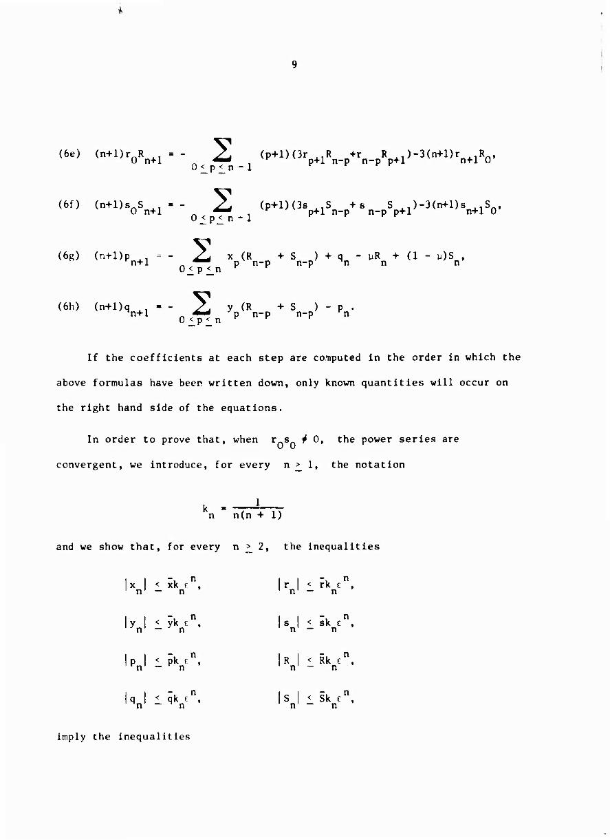
(be) (n+l)r R 1 nR ,, - - ^L (p+l)(3rAlR +r R ^.i )-3(n+l)r . .R., 0 < fi^i - 1 P n'p n~p P

(6f) (n+l)s0Sn+1 « - 2 , (P+^^s^S +s S ^-aCn+Ds^S^ 0iPln"1

(6g) (n+l)p .. = - ^ x (R ^ + S ,,) + q^ - uR,, + (1 - u)S . n+1 - ^"^ p n-p n-p n n n 0lPln

(6h) (n+Dq^, - - ^ y„(R__^ + s_.) - p„. p

'n+l n ^* 'P" n-p n-p' "n 0<p<n

If the coefficients at each step are conputed in the order in which the

above formulas have been written down, only known quantities will occur on

the right hand side of the equations.

In order to prove that, when Tnsr. t 0» the power series are

convergent, we introduce, for every n > 1, the notation

n n(n + 1)

and we show that, for every n > 2, the inequalities

x < xk f , r ' < rk c , n1 — n ' n1 - n

y i < yk e , | s | < sk e , ^n1 — ' n ' n' - n

|p | < pk fn, |R | < Rk cn, rn — n n — n

q | 1 qk E", |S | 1 Sk cn, n n n n

imply the inequalities

10

I (7a)

(7b)

I -u n+1

n+l

(7c) < rk n+l

n+1' — n+1

n+1 yn+lllykn+le ' (7d) |sn+l' -^n+l^' '

(7«) iPn+1l lPkn+1cn+1. (7e) |Rn+1l lRkn+1cn+1.

(7h) IVll l^n+l^1' (7f) lSn+ll ^kn+l^n+1-

Dealing first with (6a), we obtain

(n + l)|xn+1| 1 (p + y)knen.

hence a sufficient condition for the validity of (7a) is that

(p + y)k r < (n + l)xk c n — n+i

Since

n n+2 (n+l)kn+1 n(n+l)

1 2 2 for n > 2,

the more rigid inequality

(8a) 2,- * -x j(p + y) 1 ex

is also a sufficient condition for the validity of (7a)

12

so that

and

n + 2o - ~(n+l) n — 3

n + 2o 11 4(1 - -4-7) < 5/3, n + 3 - 3V 0+3'

Consequently, (7c) is verified if

(8c) |(x2 + y2) + (M + |x0I)x + |y0|y <_ (r0 - |f)r.

By symmetry, from (6d) we obtain as a sufficient condition for (7d)

that

(8d) |(x2 + y2) + ((1 - u) + |x0|)x + |y0|y '_ (s0 - ^)s.

We now address ourselves to (be). Using the same relations and the

same estimates as in the preceding case, we find that

(8e) 3R0r <_ (r0 - ^F)R

is a sufficient condition for (7e), and by symmetry that

(8f) 3S0i 1 (s0 - 22i)S

is a sufficient condition for (7f).

At last we examine (6g). We give it the form

(n+Dp ^. ' -x(R +S ) - x (R„+Sn) + q - uR + (l-u)S - S* x (R +S ) rn-H Onn nOO 'n n n, Ä— , p n-p n-p 1< p < n-1 r r r ^ x (R

13

so that we come to the inequality

(nM)!p J < k c [(R + S)|xJ + (Rn + Sr.)x + q + MR + (1 - u)S]

1 <^p j^n-l r

Therefrom we deduce that a sufficient condition for (7g) is the Inequality

kn[(R+S) x0 + (R0+S0)x + q + UR + (l-u)S] + x(R+S) ^ k k _ ! (n+l)k pt . . , P n-p — n+1 1 < p < n-1 *

But the identity

n + 1 « (p+l)(n-p+l) - p(n-p)

implies that

(n+i)k k . 1(1 + -i-) . -Irc-rr + -^rr) p n-p n p n-p n+2 p+1 n-p-H

and hence that

1 2(n-l+2o ,) (n+1) Z^ k k

l-Pl""1 P n"P n(n+2)

However,

o . < n-1, n-1 — '

14

which implies that

n-l-»-2o — < 3(1 - -) < 3,

n - n

Therefore, a sufficient condition for (7g) is that

(8g) |[(R + S)|x0| + (R0 + S0)x + q + uR + (1 - M)S] + 3x(R+S) <, pc

By symmetry from (6h), a sufficient condition for (7h) is that

(8h) |[(R + S)|y0|+ (R0 + S0)y] + 3x(R+S) ± qt.

Now that we found sufficient conditions to be fulfilled in order that

the inequalities should be fulfilled recurrently, we have to check that they

are compatible.

To begin with, ( can always be chosen so large that (8a), (8b), (8g)

and (8h) are satisfied no matter what values the constants possess. Also,

it follows from (8e) and (8f) that we must choose

r < 3r0/20, i < 3s0/20,

after which (8e) and (8f) are satisfied provided that we choose R and S

sufficiently large. After this, (8c) and (8d) will be satisfied, if we

choose x and y sufficiently small in comparison with r and s. In

thus choosing small values for x and y, we do not run into difficulties,

because the inequalities (7) show that small values of these constants can

15

be compensated by choosing t sufficiently large.

The inequalities (7) being satisfied for any n >_ 2, the recurrent

series (6) are dominated each by series of the form

+ Bt + C 2dk tn

tn,

n >_2 n

which is convergent in the disk |t( < 1/t. Thus the series (6) are

convergent in this disk.

3. VARIATION EQUATIONS

We denote by the vector 6 the displacements (fx.cW.^p ,^p ) of x y

a solution t ♦ (x(t),y(t),p (t),p (t)) of the canonical equations (3).

This vector is determined by the vector variation equation

(9) A = V(t)<S.

V(t) is a 4 » 4 matrix function of the form

(10)

wherein

(11a) a(t) = - ;(t) L ^(t) j P2

3(t) [ p2(t) j

16

(llb) p(t) . 3 -i^L. CxL^Ll ,)y(t) + 3 _±__ (x(t; ^- l)Y(t) ^

Pj(t) pj(0 P^t) P2(t)

(He) Y(t) pj(t) L P^Ct) J p^t) [ P2it) J

The variational equations (9) are the canonical system derived from

the Hamiltonian function

(12) ^V» '^P2 + V) - ('^p - 6y(Sp ) - '.[.(t)^2 + 2e(t)(Sx6y + Y(t)6y2l. rxy y x

Because the original Hamiltonian function (1) is conservative, the

equations (9) verify the Jacobi variational integral

(13) r = ^ x •-— + ^ v • — + ; p • + p • )X tv x tp v 'P

x y

where the coordinates and momenta in the partial derivatives should be given

their values at each time along the orbit.

It is our purpose to show that the variational equations can be integrated

by recurrent power series together with the equations of motion.

For simplicity we think of our task as two-fold. At each step of the

recurrence, we first compute the coefficients in the power series representing

1,1« and y. Then by means of the variational equations, we compute the

17

corresponding coefficients in the power series represent-?ng the displacements.

The recurrent power series expansion of a,3,7 requires several

auxiliary variables. The selection may vary widely according to one's

prejudices and predilections in programming; it might also be influenced by

the kind of mathematical information one would like to draw on the side from

the integration. We present here a list yielding fairly elegant recurrence

formulas. Our own eoniputer program actually uses a list with four less

auxiliary variables needed. Here we introduce in a first block

• A * ^-^ , B » -X "^ ' 1 . C - -^ , D - ^ pl p2 Dl P2

and in a second block

E « 1 - 3 A2, G - AC, J - 1 - 3 C2,

F = 1 - 3 B2, H - BD, K - 1 - 3 D2.

so that the time dependent coefficients in the matrix V take the simple

form

u « -(RE + SF),

t3 * 3(RG + SH),

Y ' -(RJ + SK).

We denote the coefficients in their power series in the natural way:

= X A (At)". ^"T» n

A ■ ^^ A (At) , and so on. n 0

18

As for the variations themselves, we have put

6x - \ i(Lt)nt 6px - 2* ^n(

At)n. n^^) n >_ 0

6v " ^rf nn(At)n, <Sp - 2L *n(

At)n. n > 0 y n > 0

For n « 0, the coefficients in the auxiliary series A to K and In the

functions, a,ß,Y are computed from the initial conditions on the orbit, while

they are determined in the variations from the chosen initial values for

the displacement. Once the coefficients of degree n have been computed

for the coordinates and momenta along the orbit, and the displacements to

the orbit, the coefficients of degree n + 1 are computed by means of the

formulae (6) to be followed by four new sets of formulae. The set that

ought to be handled first is

(14a) r An - x - A r A , On n ,, ^■" . n-p p 0^p^:i-l K '

(Ub) s B - x - Sj s B , On n n *** , n-p p

0 < p < n-1

^ r C , *■■ n-p p

(14c) rnC - yn - < On n ^" n-p p

0 < p < n-1 '

(14d) snD^ « y„ - ^ s__„D_; On ^n rt "^ . n-p p

0 < p < n-1 l '

then, the recurrence should go through the formulae

19

IK (15a) E = -3 ,Zj A A • <15b) F = -3 7. ii Bn . n n ^* p n-p n _ ^^ p n-p Opn 0^p<n

1

(13c) G - y. AC , n ,, ^^ p n-p

0 < p ^ n 1 (13d) H 2 B D

n ^ — P n-p 0 < p < n

1 0^Pln (l^p^n

2 before the coefficients of the time functions in the matrix V could be

computed by

(16a) *«- y. (RE +SF ) , n n ^*_ p n-p p n-p

2 (16b) ß = 3 S. (RG + S H ), n n ~

m p n-p p n-p 0<p<n K

2 (16c) >=- vf. (RJ +SK ). " 0 T- n P n"P P n'P

FinalIv the coefficients of degree n in the variational solutions are

given bv

(17a) (n + IK J_1 • n + * , n+I n n

(17b) (n + l)n ^^ = -f + . , n-»-J n n

20

(17c) (n + l)i = , + X (» : + r n n) , n+1 n ,, ^" p n-p p n-p

0 » p •' n '

C17d) (n + 1 ),,,,, = -:„ + ^ (• ..■.._„ - »..• ..) n+1 n - **^ p n-p p n-p 0 < p < n !

A proof of the convergencL' for the series in the variations follows

the same lines as the proof we gave in the first section of this paper.

4. CHARACTERISTIC EXPONENTS

We consider the four solutions A ,<5 ,6 ,6 of the variational

equations which are determined respectively by the initial conditions

'x^O) = 1, dy^O) = 0, 6p*(0) = 0, V (0^ = 0,

•xII(o) = o, ^vII(o) = i, .ipII(0) = 0, ^"(O) = 0, x y

ixIII(0) = 0, lv1II(0) = 0, 'p111^) = I, ipIII(0) = 0, x y

IV IV IV IV ■x (0) = 0, V (0) = 0, <Sp (0) = 0, vp (0) = 1.

X V

We call R(t;0) the matrix whose columns are made of these four solutions;

this is nothing else than the matrizant of the variational equations such

that

R(0;0) = \k

(I. denotes the 4 ' 4 unit matrix.) 4

26

2 or, since S ■ I., the identity

^(SR(-t;0)] = V(t)lSR(-t;0)].

Hence, using again the fact that R(t;0) is the natrizant of the variation

equations, we come at last to the identity

(23) SR(-t;0) = R(t;0)S.

In particular, at time t ■ T/2,

SR(-T/2;0) = R(T/2;0)S.

Therefore, the determinantal equation (20) takes the form

(24) det(R(T/2:0) - sSR(T/2;0)S] - 0;

it proves that the computation of the characteristic exponents for a

symmetric orbit requests the integration of the variational equations over

only half a period.

This proposition has been stated first by Moulton (1914); but the

proof he gives for it depends too closely on the particular problem he is

dealing with, namely the orhital stability of Jupiter's satellite VIII, and

it is incorrect on several points, de Vogelaere (1950) has shown how to

use it for extracting numerically from Hill's equation the characteristic

exponents of a symmetric orbit. We now propose to do the same for the

solution of equation (24).

27

First we observe that the matrix identity (23) is equivalent to the

scalar identities:

^xI(-t) =

I

^xI(t),

Av'(-t) = -V(t),

^D^-t) = X

y

-6px(t).

II, , II X (-t) = -(SX

6yn(-t) - 'v"

II. , II 'p ("t) = tp

X X

II, . II

dx111^) »

I III, , (Sy (-t) =

III , v ^x (-t) =

. Ill, v 6p (-t) =

III, . ■6x ^t).

'yin(t),

x ni, v 6px (t).

Ill, v •<Sp (t).

^xIV(-t) =

^yIV(-t) =

*pIV(-t) = X

'p (-t) = V

tx

-i v

-Al

t),

t),

t),

t).

V (t).

(t).

(t),

VV(t) V

Therefore, the determinantal equation (24) can be written explicitly as

(25)

1 II (l-s)^x (T/2) (l+s)^x (T/2)

I

(H-s)ApI(T/2)

(l-s)^pI(T/2) y

II (l+s)V(T/2) (l-s)^v (T/2)

(l-s)>II(T/2) x

(l+s)^II(T/2) v

(l+s)lxII1(T/2)

(l-s)WIII(T/2)

(l-s)ApI1I(T/2) x

(l+s)ApIII(T/2) v

(l-s)AxTV(T/2)

(l+s)'v1V(T/2)

(l+s)pI\T/2)

(1-s) p'V(T/2)

= o.

We put

(1,2) (3,4)= [ ^xI(T/2)AyIV(T/2)-'xU(T/2)^vI(T/2)]

[(SpII(T/2)ApTII(T/2)-lpni(T/2)-pII(T/2)l,

X V X V

28

(l,3)(2,4)-(6xI(T/2)6pIV(T/2)^xIV(T/2)6p^(T/2)]

[^yII(T/2)6pIII(T/2)-6yIII(T/2)^pJI(T/2)l.

(l,A)(2,3) = ((SxI(T/2)^pIV(T/2)-6xIV(T/2)6pI(T/2)]

[6yII(T/2)6pIII(T/2)6yIII(T/2)6pII(T/2)], Ä X

(2,3)(l,4)-[6yI(T/2)6pIV(T/2)-6yIV(T/2)6pI(T/2)I A A

[6xII(T/2)6pIII(T/2)-6xIII(T/2)<SpII(T/2)l,

(2,4)(l,3)«[6yI(T/2)6pIV(T/2)-6yIV(T/2)6pI(T/2)]

[6xII(T/2)6pIII(T/2)-6xIII(T/2)6pII(T/2)], A A

I IV TV I (3,4)(l,2)«[Ap1(T/2)6plV(T/2)-6pLV(T/2)6p1(T/2))

X y X y

(6xII(T/2)6yIII(T/2)-6xIII(T/2)6yII(T/2)l

so that the determinantal equation (25) takes the form

(26) (l+s)4(2,3)(l,4)+(l-s)4(l,4)(2.3)+(l-s2)2

[(1,2)(3.A)-(1,3)(2,4)-(2,4)(1,3)+(3,4)(1,2))=0

In this form we see that. In order for the characteristic equation to have a

root equal to -fl, it is necessary and sufficient that

29

(27) (2,3)(1,4) = 0.

Moreover, the matrix R(T/2;0) has a determinant equal to +1. This

determinant being obtained by making s ■ 0 in (26), we obtain the

relation

(28) 1 - (1.4)(2.3) « (1.2)(3.M - (1,3)(2,4) - (2.4)(1,3) ♦ (3,4)(1,2)

In view of (27) and (28), the characteristic equation (26) takes the

simple form

(l-s2)|(l-s)2(l,4)(2,3) + (H-s)2(l-(l,4)(2,3))| - 0.

Consequently, the non-trivial characteristic roots are the solutions of the

quadratic equation

1 + 2(1-2(1,4)(2,3)]s + s2 - 0.

As in the general case, we write these two roots as

Sj -je s2 - Je

with j - 11, so that

(29) 1 + j coshCT - 2(1,4)(2,3).

There ensues from it information concerning the stability of a symmetric

periodic orbit; the conclusions are summarized in Table II.

30

TABLE II. VARIATIONAL STABILITY OF A SYMMETRIC PERIODIC ORBIT

AS DEFINED BY ITS MONODROMY AT HALF THE PERIOD

n

(M)(2,3) > 1

(1.4)(2.3) - 1

1/2 1 (1,4)(2,3) < 1

0 < (1>4)(2,3) 1 1/2

(l.A)(2.3) - 0

U,4)(2,3) < 0

real

0

purely imaginary

purely imaginary

0

real

+1

+1

+1

even instability

indifferent case

even stability

odd stability

indifferent case

odd instability

6. RABE'S TROJAN ORI.ITS

In order to numerically calculate the orbits described in this section

a double precision FORTRAN IV program for computing asymmetric periodic orbits

in the plane restricted problem of three bodies was run on the IBM 7094 computer

In addition to calculating the basic dependent variables of an orbit with given

initial conditions, the program provides for the calculation of the four in-

dependent solutions 5 ,6 ,6 , and 6 of the variational equations. If

(for a given value of the period) the initial values are such that the orbit

is truly periodic, the characteristic roots of the periodic orbit may be

calculated. If the orbit is not as close to being periodic as may be desired

31

(i.e., if either |x(T) - x(0)|, |y(T) - y(0)|, |px(T) - Px(0)[, or

|p (T) - p (0)| are larger than some given constant, such as for example

-8 -10 10 or 10 ), then the program provides for changing the initial

conditions slightly so that an orbit will 1 obtained which is closer to

bting periodic with the given period T. Of course, reasonable approximations

to the initial conditions are necessary; it is not expected that the program

will be asked to find a periodic orbit of given period starting with arbitrary

guesses for initial conditions.

In order to explain this method of "improving orbits to make them truly

periodic" some simplifying notation will be used. Let xCtiXp,) represent

the vector whose four components are x(t;x ,y ,p ,p ), y(t;x ,y ,p ,p ), X0 y0 U U X0 y0

p (t;x ,vn,p ,p ) ^nd p (t;x ,y ,p ,p ), where these four variables 0 ^ y u u x0 y0

represent the soluticn of equations (3) with the particular initial conditions

>I -* -»II -»■ »III » tlV -♦ (x0,y0,Px ,p ). Similarly, 6 (t;x0), 6 (t;x0), i (t,x0), * (tJX0) represent

the f^ur linearly independent solutions of the variational equations. For the

given period T, it is assumed that

x(T;x0) * x(0;x0)

although these vectors are not "too far" from being equal. Considering the

first crdei variations, it is desired to consider solu:ions of the form

'30) xitiK0 + %) « x(t;x0) + OL1 61 (t;x0) + a26n(t;xu^

/ill, -» N . Jv. > , + a36 (t;x0) + a46 (t;xo)

where Av« has components Ax.,, Ay_, '.p , Ap

32

Setting t ■ 0 and remembering the initial conditions (18), it is seen

that one must have

a1 - Ax0

a2 " Ay0

a - Ap X0

a « Ap . 4 yo

If it is decided to use the given period T as a fixed quantity, then it

will be desired to have the solution satisfy the conditions

x(T;x0+ Ax0) « x(0;x0+ Ax0) = x0 + Ax0.

Substituting this and equations (31) Into equations (30) gives the results

(32) x0 + Ax0 = x(T;x0) + AXQI^T;^) + hv06Ll(lix0) + Apx 6II1 (T;^) + Apy 6IV(T,x0)

->• These linear equations are solved for the components of the unknown Ax^. If

-► -»

the new guesses xn + Axn for initial conditions still do not produce a

satisfactory periodic orbit, the process may be repeated. There is, however, a

limit on how extremely close to a periodic orbit one can come by means of this

iterative procedure. In general, we found that with 16-place arithmetic we

could ensure that no component of x(T,xn) would differ from the corresponding

-♦ •♦ -10 component of x(0.Xo) by more than 10 . However, if much better initial

guesses are known and used, the equations (32) become extremely ill-conditioned.

33

If we had an exact periodic orbit, x, would equal x(T;xn), and

equations (32) would become precisely equations (20) with s ■ +1. That

is, if we try to solve equations (32) under these conditions, it means that

we are trying to find an eigenvector (corresponding to the known eigenvalue

+1) for the matrix R(T;0).

In describing his Trojan orbits, Rabe uses a jovicentric synodical

coordinate system. The mass of the sun is taken as unity and the period of

Jupiter is 27T*/1-U. If we use asterisks to represent variables used by Rabe,

the transformation equations giving our units in terms of Rabe's are

x * 1 - u - x*

y = -y*

dt dt*

^-T* /1-u

C - (l-u)C*.

The orbital values given in Tables I and II of Rabe (1961) and Tables I and II

of Rabe (1962) were transformed by means of these equations and by the equations

dx Px" dT" y

r y dt

34

to give the Initial values in Table III and the values of T and C given

in Table IV.

In each case, the period T as given in Table IV was taken as a fixed

parameter, and a more accurate periodic orbit was calculated as described in

the preceding paragraphs. For these new orbits, the characteristic roots

were calculated. In Table V are given the new initial values for the periodic

orbits. Table VI lists the Jacobi constant as well as the trace of the

monodromy matrix and the characteristic roots corresponding to the periodic

orbit.

35

TABLE III. STARTING VALU-S FOR PERIODIC ORBITS--fabe'S results transformed (to the units of this paper

Rabe's Perameter

d o

xo ^0 ^0 Vo .0025 .500296124643 -.868190470 .864939351691 .498421029587

.0030 .501546124643 -.870355530 .863857161536 .497798523295

.0075 .502796124643 -.872520600 .862778849534 .497178495820

.0100 .504046124643 -.874685658 .861704291736 .496561161060

.0125 .505296124643 -.876850720 .860633590098 .495946217159

.0150 .506546124643 -.879015780 .859566642668 .495333906001

.0175 .507796124643 -.881180850 .858503443453 .494724073660

.0200 .509046124643 -.883345912 .857444086401 .494116614187

.0225 .510296124643 -.885510980 .856388739438 .493511365658

.0250 .511546124643 -.887676040 .855340133254 .492908300088

.0275 .512796124643 -.889841100 .854287389045 .492306843750

.0300 .514046124643 -.892006166 .853245632595 .491707425438

,0400 .519046124643 -.900666420 .849111400136 .489392102889

.0500 .524046124643 -.909326674 .844638938108 .487334093530

.0600 .529046124643 -.917986928 .840686966660 .484695798129

16

TABLE IV. PERIODS AND JACOBI CONSTANTS (using initial conds. in Table III)

Rabe's Parameter

"o

.0025

.0050

.007 5

.0100

.0125

.0150

.0175

.0200

.0225

.0250

.0275

.0300

.OAOO

,0500

,0600

Period

T

78.1182A642410334

78.21241134561734

78.37095698004493

78.59711486899776

78.89553723182391

79.27284722811138

79.73765896723368

80.30133787108203

80.97856094134159

81.79018812928275

82.75360773001720

83.91284074382773

91.82099333962959

117.7920128526034

183.5145658929861

Jacobi Constant

3.0000046197401

3.0000184246002

3.000041333/195

3.0000732673572

3.0001141457676

3.0001638928252

3.0002224296547

3.0002896819513

3.0003655816422

3.0004502334866

3.0005428247134

3.0006443168953

3.0011363774494

3.0017245907688

3.0024430527304

37

TABLE V. STARTING VALUES FOR PERIODIC ORBITS (PRESENT RESULTS)

Rabe's Parameter

do (approximate)

1.0025

1.0050

1.0075

1.0100

1.0125

1.0150

1.0175

1.0200

1.0225

1.0250

1.0275

1.0300

1.0400

1.0500

1.0600

0 '0 ^O

500294701009 -.868189394186 .864940407774

Vo

,498420857938

.501546202315 -.870355763449 .863857082677 .497798432577

.502795932420 -.872520424844 .862778961872 .497178566762

.504046133194 -.874685581794 .861704299953 .496561215540

.505296118194 -.876850529922 .860633607448 .495946396251

.506546050763 -.879015868171 .859566684583 .495333815576

.507796128489

.509045980033

.510296189709

.511545765989

-.881180842237 ,858503483592 .494724052434

-.883346025885 .857444171146 .494116467086

-.885510985492 .856388586745

-.887676141744 .855340268383

.512795779277 -.889841341844 .854287586217

,493511547160

,492908273233

,492306477874

.514045824807 -.892006380486 .853245786222 .491707120286

.519045209040 -.900666970996 .849111898087 .489391219068

524045017193

529053778602

-.909327242850 .844639557053 .487333137683

-.917980837710 .840684004699 ,484703533306

38

TABLE VI. JACOBI CONSTANTS, TRACES, AND CHARACTERISTIC ROOTS USING

INITIAL CONDITIONS FROM TABLE V AND WITH SOME PERIODS AS

IN TABLE IV

Rabe's Parameter

d0 (approximate)

1.0025

1.0050

1.007 5

1.0100

1.0125

1.0150

1.0175

1.0200

1.0225

1.0250

1.0275

1.0300

1.0400

1.0500

1.0600

Jacob! Constant

C

3.OOO0046137 301

3.O0O0184264690

3.OOO0413312188

3.0000732665714

3.0001141435380

3.0001638941519

3.0002224306764

3.OO02896834712

3.0003655812550

3.0004502346940

3.0005428266252

3.0006443182264

3.0011363784399

3.0017245910778

3.OO24430503909

Trace

.43885321

.32970410

.17882263

.04109871

.00832747

.21110820

.79229906

1.81711725

3.09222181

3.96383295

3.44565407

1.33281279

.11223160

1.17049332

4.07526522

Characteristic Roots

-.78057339 ♦ .625064141

,83514795 1 .550025371

91055869 l .413313741

97945065

-.99583627

■f 9 201683991

,091159931

-.89444590 1 .447176171

,60385047 797097621

-.09144138 1 .995810461

54611090 1 .837712891

,98191648 t .189314641

72282704 ♦ .691029001

33359361 t .942716981

-.94388420 1 .330276581

-.41475334 1 .909933881

1.3145467 and.76071849

39

» I Fig. 1. Variation 6x for Trojan Orbit (C = 3.0000603664498 and

T = 78.505049A8179581) versus time (the unit of time is the

period T).

40

The orbits described by the parameters in Tables V and VI are

practically the same as Rabe computed. The only reason we refined them

slightly using our methods and lb-place arithmetic was to enable us to

calculate the characteristic roots with good accuracy; this point will be

discussed later. The fact that the entries in Table V are quite different

from corresponding entries in Table III does not mean that the orbits

themselves are very different; our iteration method has merely allowed for

starting at a slightly different point on the orbit. The only real difference

between the orbits is due to the fact that we took Rabe's 5-decimal place

value for the period as being an exact constant, and found the more accurate

orbit which has this exact period. Another indication that there is not too

much difference between Rabe's original orbits and our modified ones is that

the Jacobi constants as given in Table IV do not differ from the new Jacobi

-9 constants as given in Table VI by more than 6 » 10

In the way in which our computer p'ogram was used for the cases represented

in the tables, the number of terms of the series was fixed at from 16 to 20.

The step size was then determined so that none of the last three terms in any

of the series would be more than 10 . At the end of the orbit, the number

of terms taken in the series might in some cases be diminished in order to keep

underflow from occurring. We considered an orbit to be periodic if no

> > component of >(T,xn) differed from the corresponding component of ■(0;. ) *

by more than 10 . The Jacobi constant associated with the solution of the

equations of motion remained the same to fifteen significant figu.es. The

41

Jacob! constants associated with the variational equations remained the

same to eleven deciral places. The equations(19) were satisfied with

-9 residuals at most 10

In integrating the equations of motion it is feasible to use other

methods of numerical integration, although probably more machine time

would be involved. The power series method becomes relatively more

advantageous when integrating the variational equations. The solutions

of these equations are highly oscillatory in nature, and a high order

numerical integration method is essential if an extremely small step size

and multiple precision in adding on the increments is not to be required.

Figure 1 shows a sketch of the four components of one variational equation

solution. The points showing on one curve are those which were required

to be calculated by the power series method using 16 terms of the series.

(In actually drawing the curves. Intermediate points were also calculated

so as to present the true shape for Illustration.) Since the basic orbital

variables occur In the variational equations, the step size required for

integration of the variational equations Is then the step size for the whole

problem when the Integrations are done together in an efficient manner.

In many types of problems, loosely approximate solutions of variational

equations may be sufficient, but In thl? rase it is Imperative that the values

of the four variational solutions be kno^r "Ight at the end of the period.

Because of the rapid changes in the four solutions, the trace of the .»atrlx of

the solutions also changes rapidly, and the calculated characteristic roots

would not be correct If the orbit were not very close to being periodic and 11

the variational equations were not solved very accurately. In order to be

42

absolutely sure that the accuracies described in the previous paragraphs

were indeed good enough to permit determination of the characteristic roots

accurately, we chose initial conditions which were approximations to

orbital values at various parts of the orbit. When truly periodic orbits

were obtained using these initial conditions as first guesses, it was found

that the calculated characteristic roots were the same to eight decimal

places as t ey were when a start was made at a different point on the orbit.

In accordance with the criteria given in Table I, the results in

Table VI show that all of Rabe's orbits are stable except the last one. The

stable orbits are of oval shape. The one unstable orbit is of horseshoe

shape. It is evident from looking at the columns listing the trace and

the characteristic roots that as the periods of the various orbits increase,

the characteristic roots travel around on the unit circle. There will be

points of "indifferent stability" as indicated in Table I when the path of

the roots actually hits the point -1 or 41.

r \

)

• BLANK PAGE

I

45

APPENDIX: COMPUTER PROGRAM WRITE-UP

Program 36 - "Non-symmetric orbits with variational solutiuns"

1. General Information

A. Purpose

The purpose of this program is to calculate accurate

periodic orbits in ehe plane restricted problem of thrre

bodies. Four independent solutions of the variational

equations may also be computed so that the characteristic

roots associated with the orbit mav be obtained.

B. Restrictions

1. This is a FORTRAN IV program which has been run on

an IBM 7094 under the IBSYS system in which tape 5 is the

input tape, tape 6 is the output tape for printing, and

tape 14 is the output tape for punching.

2. All input variables are either fixed point numbers or

double precision floating point numbers.

3. For a desired orbit the exact period must be j^iven.

Approximate initial values of x,y,p , and p are also

required; arbitrary starting values will in general not be

good enough.

4. If one asks for extreme accuracy in finding a periodic

orbit, the program will obtain orbits which are closer and

closer to being periodic for a while, and then next orbit

46

or orbits will not be so good again. The reason for

this is given on page 34. Thus if guesses for initial

conditions are originally extremely good, the next

supposedly improved guesses will not be as good. In

this regard, the values of the FORTRAN variable C7 has

the effect of determining whether or not these factors

are a problem in a particular case.

C. Method

1. Mathematical Method

This is described in the main body of the document.

However, as stated there, some of the actual equations

used in the computer program are slightly different from

those given in the body of the document. There are 4

dependent variables in equations (3); in the 4 independent

solutions of the variational equations (9) with initial

conditions (18), 16 more dependent variables occur. In

using the recurrent power series method for solving the

20 equations, we here introduce 13 auxiliary variables as

follows (instead of 17 as described earlier):

48

(35)

w

g

h

C

D

R

x + 2 ux + VJ

xy + uy

2 a + y

1/w

1 w - 2x + (1 - 2^)

1 - 3ga

1 - 3ha + 6hx - 3(1 - 2u)h

gd

hd - hy

(1 - u)g

L3/2

L = RA ■♦■ SB

N - 3RC ■»■ 3SD,

(36)

it is seen that in most of the definitions the right-hand

side only consists of linear combinations of products or

quotients of at most two of the other variables. In the case

of R and S, the equation may be differentiated so that

2KR - iR*

2hS =• 3Sh

49

which will also be satisfactory for the recurrent power

series method.

In all we have 33 variables to consider, (20 desired

dependent variables as well as the 13 auxiliary variables

discussed above). Each of these variables is considered

as a power series. For example.

and n » 1

n-1

-2 x <At)n"1- ^■4 n n-1

If convenient, the coefficients of the power series use

the same symbol as the dependent variable itself but are

subscripted with an n. The exceptions to this show up

in the definitions

x ^"r n n

n-1

n»l

-1

6x (i) -2 k(i)(At)n-1, i - I,II,III.IV,

*v (i) r^Cfit)"" , i - i,ii,in,iv, n

50

6p (I) u (At) n

i - 1,11.II.IV.

6p n-1

i - I.II.III.IV.

When these power series are substituted into

equations (35) (or (36)] and into the equations of

motion (3) and in the variationai equations (9). and

the corresponding powers of At are equated, the

following recursion formulas are obtained:

(37.1)

(37.2)

nx . ■ p + y n+l n n

n>r . ■ q - x n+l ^n n

(37.3) a ., ■ 2nx .. + 7. x^ ._ n-fl n+1 +*4 j n-»-2-j

(37 .4) w aa + S v y n+1 n+l 4-4 yJyn-»-2-J

(37.5) g n+l " " w, +4 Wj8n+2-J

1 "'-•

(37.6) h , • h. ,£. (2x4h A- . - w4h A- J ml 1 +*i j n+2-J J n-»-2-j

51

(37.7) Rn+1 - Y^K+l'l " n ^^j+l^l-j-^j + lVl-J

(37.8) S n-»-

1-^J3hn+1S1-iUJ12SJ+1hn+1.J-3hj+1Sn+1.j

(37.9) dn+, ' ^n+1 + & XjVn^-j

(37.10) An+1 - "3 Zu «jV2-j

(37.11) Bn+1 B ., = -3(1-2.)h_1 - 3 ^ (hja^.j - 2hjxn+2.j)

n+1

(37.12) Cn^l * ^ KlWj

(37.13) Vl ' ^^j'n^-J " VnW

(37.14) ^ « ^ (Vn^^j ^ SJV2-J)

(37.15) N^ N ., - 3Z.(RjCn+2.j +S

JV2-J)

(37.16) np - q - uR ♦ (l-u)S - 2d (R1 ^ S1 ^n+l Mn n n *^ J J )x

n-H-j

52

(37.17) nq n+1 -pn- (RJ + ^^n.l-J

(37.18) nk (i) n+1 n n i - I,II,III,IV

(37.19) n,(i)._k(i)+v(i). n+1 n n 1 - I,II,III,IV

(37.^0) nu n+1 n

(37.21) nv (1) n+1 n

k(i) +,>N£(i)

j n+l-J +^Nj£n+l-j'

1 - I,II,III,IV

+ ^N k(1) + X^jkn+l-j. 1 - I,II,III,IV,

The known initial conditions are the quantities v v^p ,

(38.1) a1 - (Xj + u)'

(38.2)

(38.3)

wj " a1 + y1

g1 - 1^

(38.4) 1 w1 - 2x + 1 - 2u

(38.5) «!-(!- u)g1 ^

53

(38.6) S « uh1 /h^"

(38.7) d1 - (x1 + u)y1

(38.8) A1 • 1 - 3g1a1

(38.9) Bj - 1 - 3h1(a1 - 2x1 + 1 - 2^)

(38.iO) C1 - gldl

(38.11) D1 - hl(d1 - yj)

(38.12) L1 - R1A1 + SJBJ

(38.13) N1 - 3(R1C1 + S^^

Now equations (37) may be used in the order listed to

obtain the second coefficients In each series, etc. When

the program is> being run in the mode in which cnly the

equations of motion (and not the variational equations) are

being solved, equations (37.9) through (37.15) and

equations (37.18) through (37.21) as well as equations

(38.7) through (38.13) are not tsed in the recurrence

process.

For the mathematical method of improving the "periodic"

orbit and for obtaining the characteristic roots associated

with the periodic orbit, see the explanation in the main tody

of the document.

54

2. Coding Method

IBM 7094 FORTRAN IV. This program and its subroutines

make maximum use of COMMON storage. We have desired to run

many similar types of problems without changing much of the

program. For this reason there are many COMMON variables

available which w*»re not actually used in this version of

the program. These show up as being undefined in the listing

of what each COMMON variable represents.

COMMON Variables

Note; A(1,I) thru A(9,I) are usually as defined below.

However, at the end of the orbit under the control

of subroutine ENDOR, they are used as matrix elements.

A/I T\ *u A/io TN i1 „I I I ill „II II II A(1,I) thru A(12,I) x^y^p^q^ k^^.Uj.v^, l^ .^ ,ui ,v1

AZ-IT T\ -U A/O/ T\ .^I »U! HI HI , IV „IV IV IV A(13,I) thru A(24,I) l^ tii ,ui ,vi , k^ ,ii ,u1 ,vi , a^w^g^*^

A(25,I) thru A(33,I) R^S^d^A^ Bi,Ci.Di,Li Ni

A(34,I) thru A(49,I)

A(50,I) R1 + S1

B(l) thru B(12) x,y,p ,p , 6x ,6y »6p ,6p , 6x ,6y ,^p ,6p y x y x y

p/i^ *u D/onN x in x m x in x m x IV . IV IV IV B(13) thru 8(20) 6x ,6y ,6p ,6p , ^x ,6y ,6p ,tp

x y x y

B(21) thru B(50)

5b

C(l) thru C(5) x(0),y(0),p (0),p (0), Jacob! Constant at t-O. x y

C(6) thru C(50)

E(l) Trace of monodromy matrix

E(2) Real part of 1st characteristic root

E(3) Imaginary part of 1st characteristic root

E(4) Real part of 2nd characteristic root

E(5) thru E(50)

F(I)

GI(I) i

GII(I) 1/1

S(I) (At)1'1

x(I)

y(I)

z(I) Erasable storage. (However, at the end of an orbit, z(I) _is carried to subroutine ORBIT through subroutines MATR, CUES, and ENDOR)

Cl,C2

CJ Parameter used to help determine At. (Kaking C3 smaller improves accuracy attainable). C3 is usually chosen between .1 and 1. and mostlv about .25.

58

N Running variable (N « 1,M)

Nl If Nl ■(,>, the program prints < .yi variables

at intermediate points on orU<t.

N2 If N2 ■<!• 0"Jy0H variables are calculated. (2, all 20)

N3 A counter to compare with M3

NA If N4 -|°i. subroutine PRNT | Jj n0tl called by

subroutine ORBIT.

N5 Ordinarily N5 - 0. Subroutine SETDT sets N5 = 1 when it has found a suitable At which will just end an orbit.

N6

N7 If N7

N8

Q.R

U.V.W

xl thru xlO

1; there is now no) , ., , . c I intermediate printing of ,, . . I variational quantities. 2; there is now j

N9 Max. number of times POWER may still be called.

N10

Ax0!

independent variable (time)

60

PRNT — This routine prints the orbital parameters

for the given value of t.

ENDOR — At the end of the orbit, this routine calculates

and prints residuals in checking equations (19).

It calculates and prints the trace and the

characteristic roots. Then it calls CUES —

This routine sets up equations (32). In order to

solve them it calls subroutine MATR. Tht suggested

corrections Ax , Ay , Ap , Ap are printed, and

the new values of C(I) I ■ 1,4 are set up.

The subroutine ORBIT then decides if it has obtained a good

enough periodic orbit. It transfers this information to the

main program by means of parameter Ml.

FANPR — This subroutine prints all necessary information (which

might be saved for long periods of time) about the true

periodic orbit.

The main program also punches (actually writes output tape 14)

two cards which give u,x(0),y(0).Period,p (0),p (0) in the format x y

required as input to the program.

B. Data input cards.

There are 5 input cards required for each case. Any number of

cases may be run one right after the other. The cards are as

follows: (When a quantity is given as "c.bi^rary" it means that this

61

input quantity will never actually be used in this particular

version of the program. Of course, if one wishes to always

use only this exact version of the program, subroutine RE36b

could be easily changed so as to read only the quantities

actually needed.)

Card 1: Forn.at (3D24.16) p x(0) y(0)

Card 2: Format (3D2A.16) Period p (0) p (0) x y

Card 3: Format (1^15) M * no. of terms in Taylor series

M2 » 4 or 20 (20 means variational equations also computed)

M3 ■ no. of integration steps per printing interval

M4 = arbitrary

MS ■ arbitrary

M6 » arbitrary

M7 - 1 or 2 (2 means there is to be intermediate printing of varia- tional quantities)

M8 » arbitrary

M9 ■ max. no. of times subroutine POWER may be called (i.e., the max. no. of integration steps you wish to allow without giving up on ever getting to the end of the period).

MIO = arbitrary

L10 = Max. no. of times subroutine ORBIT may be called (i.e., how manv complete orbits are you going to allow; if L10 = 0 it will run one orbit).

62

Card 4: Format (7D10.2)

Card 5: Format (4D10.2)

L9 « 0 or 1 (1 means CUES prints a dump of matrices and solutions)

L8 ■ arbitrary

L7 ■ arbitrary

Cl ■ arbitrary

C2 « arbitrary

C3 ■ parameter used to help determine At. (Making C3 smaller tends

to cut At). C3 is usually chosen between .1 and 1. and mostly about .25.

C4 ■ arbitrary

C6 - arbitrary

C7 ■ accuracy required in called orbit "periodic". This is the allowable difference between any of the 4 initial values of the dependent variables and corresponding values at the end of a period.

C8 ■ arbitrary

C9 « arbitrary

CIO ■ arbitrary

DTMAX ■ max. value of At you would ever want it to use

DSMAX - arbitrary

C. Output

Printed output depends on input parameters M3, M7, and L9.

Subroutine RE36D always prints the input data it has read. On

63

a new page will then come a table giving various orbital

profiles. (If M3 is very large, one may only get initial

values and values at the end of a period). The table will

generally be in the format

6X1 ty1 «P1 rx «P1

y c1

6X11 «y11 II

op A H 6p y

c11

A "I 6x A HI 6y , III op rx

A m y

c111

r IV ox E IV 5y A IV 6p rx A TV 6p

y cIV

6X1 ty1 «P1 Kx «P1

y c1

6X11 «y11 x II rx

A U 5p y

c11

A HI 6x A HI 6y A HI 6p rx x IH 6p

y c111

x IV 6x A IV 6y x IV 6p rx

x iv 5p y

cIV

etc.

Of course if M7 ■ 1, there will be no intermediate printing

of the variational solutions.

At the end of an orbit which the program thinks» fs truly

periodic (or even if it has been unsuccessful in really finding

a good one), the six variational equation checks are printed.

64

(These are the residues obtained when checking in

equations (19), and they should all be very close to

zero).

Next are printed two characteristic roots and the truce

of the monodromy matrix. Then are printed suggested

changes in initial values as obtained as a solution of

equations (32). Then the new initial guesses are printed.

If the program has been successful in finding an accurate

periodic orbit, one will usually not be interested in

these "suggested changes in initial valuts" or in the

"new guesses".

Fir.^lly the program prints a listing of important orbital

parameters suitable for saving as a page in a book of orbits.

If L9 » I , the print out will be interspersed with matrix

print outs by subroutine CUES. These are not labelled, and

the easiest way to see what they mean is to read the program

listing.

Punched output always consists of two cards in format

(3D24.16) giving for the latest orbit u, x(0), y(0). Period,

P (O), p (0). x v

D. Results

An example giving the print out for a particular trojar. orbit

is given in the following pages.

67

Vin«fHjt|Nf r«NP« mil ci r pKffisiON «. *, c, n, (?, o, c*, rs. C6. ci, cc a, cid

III. II, OlMAi, r^mtt. Et r>t ti. Oi f*. (9. f6, (7. F8. F9. flO, if, I.. (1. Ml, i.-V, f.Wlli CMUC, M, P, Ot «. S. T, Ut Vt W. "I. »if 1«3, X*, XS, X6, KT, «8. «"», XIO, Ylt W, YJ, V*, V5. ¥6, TT, T«, «V9, T|0, /, 11, 12, n, Mi /!>, /6, 11, I», /<>. /10

DIKtNStUN »(SO,SOI, 8(501, CISOI, CISOI, MSOIf GMSO», 1.11(501, ix(?oiO), yuoooi. mon), SISOI

CUMMON/S»'«/«, V C0>'N0N/n»'»»/4, *, C, Cl, C2, CJi C*i C5t C6, CT, Cti C9, flO. 0,

10T, o\m, nsa/u, E, fit r?t €i, t*. E5, fb, ET, E«, E9, ElO, r. ?G> f.l. Gil, f.NII. GMK1, GHUC. H, P, Of P. S« T, U, V, »n, «♦, xs, x6, «7, xs, «<», xioi »i. »ii vj. »*# »*i «V9, Y1C, Z, /I, i?i I), H, IS, lb, 17, l», /■», HO

CO^MON/INTS/I , II, J. K. »I, K?. K 3, **,, HS, R6, R 7,

»6 «I. «2. Y7, V8,

IB, 19, 110, N), M4, »15,

M8, Rl, RIO, M, f\, M7, H3, «♦, M5, Ht,. MT, MB, N9, N10

SUN

U . 11 , t?, II. 14, 15, 16, 17, 2M6, M7, "«. »O, MIO, N, Nl, M/,

1 roBH*ri6'.Ho 1 jiipirt« »

2 fORH*T(6JM0 EÄ* 1TM MOCN I

3 rOPKATlftSMO EOU 1«L MASSfS I

« FURM«T(5 3HO *M • 024 1.161

5 FO«HAT(53HO 1.16)

6 FORMAT IS^HO 1.161

7 FORMAT(56H00NE OF THE CONJUGATE COMPIF« CHARACTERISTIC ROOTS IS 120?«.161

B FORMAT(S6M0 1202*.161

9 FORMAT(56M0 102*.Ul

10 FORMATI109H0 i p sun x

11 F0RMATI17H0INITIAI VAlUtS «025.16I 12 F0RMATI1TH0 FINAL VALUES 6025.161 13 FORMATdMCI 14 F0RMATI3bH0INtT|A| 15 FORMATI7SM1

1 TMRFF ROOY PRUHlfMI MRITt16,151 |F(GMU-1.0-03120,20,25

20 HRITF16,11 60 TP AO

25 IF(GMU-.01250012^,28.30 28 MRITF16,21

GO TO 60 30 IF(GMU-.500160.35,60 15 HRMt 16,31 60 HRITF Ift.OGMU

JACOB I CONSTANT ■ 026

PERIOD ■ 026

THE TWO RFAl CHARACTERISTIC ROOTS ARE

THE IRACE HAS

II P SUB V I

DX/DT AND OY/OT VALUES MERE 2026.161 PLANE RESTRICTED

.1

.3 ,6 .6 .7 .8 .10 .11 .12 .16

.2

.9

.1)

.19 .1*

66

65

50 60 70

MRITt(6.5)C(5I MRITtIC,6IC5 MRITt(6,131 MRITt16,101 MRITt l( ,11 Mf ( 11. 1*1.61 MRITt (6,I?MB( I I, 1*1.61 n«C(2l»C(3l /2«C(4l-r(1 I MRITt t6.|6U1.22 IF IM?-*I 66,70,66 MRITf 16,131 IF(f(31 150.65,50 MRITF 16.»If m.tm GO TO 60 MRITtI6.7IEI2),EI31 MRITt (6,«»If ( 1 » RETURN ENO

.IT .IB .1«

.20 .21 .22 ,ii .26 .29 .2« .27 ,28 .2* .90 .91 .32 .93 .96 .99 .9«

O* .60 .61

.69 .66

|66 .67 .68

.90 .91 .92

.99 .96 .99

BEGIN ASSEMBLY 12.875

68

SUBKOUTINC Goes DOUBLE DECISION A. t. C. Cl. C2. CJ. C«. C5. Cft. CT. C«. C«. ClU«

10. OT. DTMtl, DSMAI. I, Cl. E2. £1. E*. E5, Cfr. ET. Et, E%, Elü, ?f. C. Cl. CII. GMU. GMUl. CMUC. N. P, 0. R, S, T. U. V. H. II. 12. 31). I«. IS, 16. IT. IS, I«, 110. Tl, V2. TJ. V«. V5, *6. VT, Tl, 4T«. T10. I. 21. 22. 23. 2«. 25. 26. 2T. 21. 2«. 210 DIMENSION AtSO.SOI. B(90l. MtOI. EI90I. fl»OI. Cl(50l. ClieiOI. 11120001. YI2000I. 2(100). SISOI COMMON/SPK/1. T COMMON/O^K/*. B. C. Cl. C. C). C*. C), C6. CT. CB. C«. CIO. 0.

IDT. OIMAI. OSMAft, E. El. E2. E). E*. ES. 16. ET, EB. E9. E10. F, 20. 61. CII. CMU, S«U1, GMUC. M, », 0. K. S. T. U, V. M. II, 12. )l). ts, 15. 16. IT, IB. I«. 110, Tl, r2, »i, V«, V5. V6. TT, YB. ♦»«, »10, 2. 21. 22. 2). 2«. 2). 26. 2T. 2B, 29, 210 COMMON/INTS/I, II, J, K. Rl, K2. R). R«. R5, R6. RT, RB, R9, RIO,

11, LI, L2. L). 16, L5. 16. LT, LB. \H, L10, M, Ml, M2, M), M«. MS. 2M6. M7, MB. M9, MIO. N, Nl. N2. NJ. N4, N5, N6. NT. N«. N9. N10

1 FORMAT()6H0SUC0ESTE0 CHANGES IN INITIAL VALUES 6020.1)1 ? FORMAT I5)H0E0U6TIONS TO BE SOLVED FO« CHANCES IN INITIAL VALUES I ) F0RMATUH0019.12,6D20.UI 7 DO B I»l, 6

DO 8 J-2, 5

8 AII.JI ■ B(RI DO 9 1-1, 6

9 All,i*ll • Afl,l*ll>l. DO 12 1-1, 6

12 All,61 ■ CII>-B(I) IF 119) IB, IB, 16

16 WRITE 16.21 MRITE I6.3M(AII.J),J>2.4I.I-1.6)

IS CALL MATR IF IL9I 29. 25. 20

20 MRITE (6.))IIAII.JI,J>2.6I,I>1,9)

25 MRITE 16.1)12111.I>1.61 21"0. ** DO )0 1-1.6 22-DA6SI2IIII _ IF 111-221 2T.)0.)0

2T 21-22 SO CONTINUE

IF 121-FI 50.90,)9 3» M.5»F

21-F/21 DO 60 1-1,6

60 2I1)-2(I)*21 MRITE 16,11 (211).1-1.61 CO IU 60

50 F-21 60 RETURN

END

.1

.2

.1

.6 .5 .6

.T • B .» .10 .11 .12 .13 .16 .15 .1* .IT • IB .1«

.22 .23 .26 .25 .26 .2T .2B .29

.32 .33 .)6 .35 .36 ,3T .3« .60 .61 • 62 .63 .6* .65 .66 .6T .6B .6« .50 .51 .52 .53 .56 .55 .5? .5B .59 .60

.20

.iO

.3B

.21

31

.56

70

6 7 e

u 12 13 I* IS

150

lib

15T 16

20

SUM OUT I HE DOUBLE ODE

10. OT, OT* if t Ci 01 }»>, t«, 15 *»«, »10, I

DIMENSION 1112000). v

CO"«»ON/SP« CO«M»0N/Df»«

10T, TTH»», 26. 01. Gil }»», 14, 15 ♦T9, V10. i

COMMON/INT U, U. L2i 2M6, MT. M8

1 FOftHAT ||H ) CALL 'OME«

CALL SETOT T»T»0T C*Ll Sf.TP« IF IN*I T , CALL PRNT IF (N<>) 11 IF «MM S. «2-* L10-0 IF t*2-*l CALL ENOOK IF IL10I 2 21-0. 00 152 1-1 L2m OAOSIC

F (21-22> 21*22 CONTINUE IF «21-C7I mimo

DC 15 7 !•' Cl I i'2( I > 110-LlO-l «EfURM «I " 1 60 TO 16

.mo

ORBIT CISION A, B, C, Cl, C2. C3. C«, C Al, nSMAI. (, El, E2, EJ, £4, E5, Oil. GMU, CMUl, GMUC. H, P. U. R, . 16, If, 18, X9, (10, VI, V2, V} I 21. 22, 2), 24, 25. 26, 2T, 2«, AI50.5ni. »1501, CI50I, EI50I, F| (20001. 2(1001, $1501 /M. * /»• B. C. Cl- C2, CJ. C*- C5. CA.

OSNAI. E. El, E2, f). 16, E5, E6 . OMu, G*U1, CHUC, H, P, Q, K, s, , 16. 17, IB, 19, 110, VI, V2, V} . 21. 22. 2), 26, 25, 26, 27. 28. S/l, 11. J. K, Kl. K2, K), K6, K5 L3, 16, 15, L6, IT, LB, L«, L10,

. M9. MIO. N, Nl, N2, N3. N4, N5, 02021.16.028.16,021.16,028.16 1

7, 6

. 11, 8 5, 12

13.16.13

0.20.15

.6 I n-niin 150.152,152

20,20,155

5, C6, CT, CB, C9, CIO. E6, ET, EB. E9, E10. S. T, U. ¥. M. II. 12.

, V6, V5, V6, VT, VB, 29. 210

50). 01(501. GI I (5W.

CT. CB. C9. CIO. 0. , ET, E8. E9. E10, F,

T, U, V, H, II, 12. , V6, V5, V6, VT, VB, 29. 210

. 16. 17. KB, H9, MO. M, «1, M2, M3, M6, mi, N6, NT. N8. N9, N10

♦Cdl

.20

.25

8E6IN ASSEMBLV 16.886

71

SURROUTINE POME« DOUBLE PRECISION «. B, C

IDt OT, OTMtX, OSMiiX, E, ?F. Cf CI, Gil, GMU, GMUl 313. «♦, I), X6. n, IB. *V9. VIO. It H, 12, M.

OI«fNSION »('O.iO), «150 11(70001. r(?OOOI. 21100) coMMON/sPR/i. y cn»««()N/opR/«. «. c, ci.

IDT. Olf»«, OSHAX. E. El. 20. Gl , GlI. GMU. GMU1. G 3X3. X4. XS, Xfc, IT. XB. *y«». no, z, n. Z2. zs,

COMMON/lNTS/l. II, J, K, 11 . 11 , L2, LI, L*, L5i L 2M6, MT, MS, "9, MIO, N,

DO 10 I>1, M2 10 «I 1.1 I • BID

Zl • BIll^GMu

. Cl. C2, CSf C*. Ci, C6, C7. CS. C«. CIO« El. E2. E3, E4, E9. E6, ET. ES, E«. EID, , GMUC, M, P. Q, R, S. T. U. V. M. XI, X2. X9, XIO, Tl, li, »3, »*. »5. T*. T7. TB, 24, 2S. 26. ZT, 2B. 2«. 210 ). CI5C1, EDO). PISOI. GlliOl, GIII50I, . SISO)

Cl, C3. C4. C5, C6. CT. Ct« C«. CIO. 0. E2, E3. t*. E5, E6, ET. E8. I», E10. P.

MUG, H. P, 0, R, S, T, U, V. M. XI. X2, X4, XIO, Yl, Y2, r3, V4, VS. T«, TT. TB, 24. 25. 26. 2T, 2B. 24. 210 Kl, R2, R3, R4. R$. R6, KT. RB, R9, RIO,

6, LT. LB, 14. L10. M. Ml. M2. MB. M*. M5, Nl, N2. N3. N4. Ni, N6. NT. NB, N4, N10

RI21.1) »127.1» »l/J.ll RI74.1I •(75.1) «176.1) »(■>C, II

1<>

2*

Z1*Z1 »(71 .1I*6I2I«B 1.IRI22.1I l./l»(72.1IM. •GMU1*»(73.1)« GMU*»(?».1I*DS tl7&.n*»(26.1

(21

-21-211 DSORI(»(73,i II C»T(»(7*, I I> 1

GO TO (70.1*1, N? »(7T,1I »(76,1 I »174,11 »MC, l i »(31.1) »(37.1 ) »(33.1)

20 00 LI L7 21 27 23

50 NM • N»l • M*2 • 0. • 0. • 0.

• 2l«B(7l • l.-3.*»(23.I)« • l.-3.«»(7<.. !)• ■ »(23.1)*»(7T.l • »(2«,1I*(»I2T, ■ »(25-<<«»(2B,1 •(»I25,ll*»i30.1

L

»121.11 (»(21.11*1.-21-211 I 1 )-6(2> I l*»(26.1 l*|(24,ll I*»:26.1l«»l3l.in*3.00

»(l.N*l) »(7.N«1) 00 2* J"i R • L2-J 21 ■ 22 • 23 - »(21, »122. 24 ■ 0. 25 - 0. 26 ■ 0.

&lI(*)•(»(3,N GIIINI*I»(4.N Ll

1*«(1.J)*»(1.R) 7*«(1.JI«»(7.RI 3*»(2.J)«»(2.RI

)«»(2.NI) )-»(l.N) I

2.*GMU**I1,L1

»I21,L1)«23 l«21

.1 ,2 ,* ,5 .6 , i ,* .4 .10 .11 .12 .19 .16 .15 .16 .17 .IS .14 .20 .21 .22 .23 .26 .25 .26 .27 .28 .24 .90 .31 .32 .96 .95 .96 .97 .98

.99

73

SUAftOUTlNf MINT DOUBLE PKCCISION «t Bt C. Cl. C2, CJ. C*, C9. C6. C7. Ct. C», CIO.

10. DT. Di»»*«. OSMAI. i. El. E2. E>. E4. E5. E». ET, ES. E«. EIO, 2F. (,, Cl. Gil. &*U. &MU1. GMUC. N, P. C. *. S. ft U. Wt M. 11. >2t )I3. «♦, It. 16. n, 18. X«. «10, Tl. 12, V). V4, »5, T4. VT, Tit *V9. vie. Z. n. 12, 2). 2«. Z9. /6, IT. II. 2«, 210

OIMENSIUN «150.501. eiiOI. CtMl. EtiOI. fCiOI. CHJOI. 611(50». 11(20001. YI2000I. 211001. SI50I CO<»W)N/$P«/x, * COMMON/DPR/A, 6. C. Cl. C2. CJ. C«. C5. C*. CT, Cl. C«, CIO. D.

IDT. OTPtt, OS"*x, E El. E2. E3, E4. (5. E*. ET. Et. Et. EIO. P. 2G. Cl. CM. GMU. &MU1. GMUC. H, P. Q, ft, S, T, U, V, M, II, (2, 313, 14, 15, «6, XT. 18: 14. 110. VI. T2. V3, V«. V5. V4, VT. T8. «v<9, TIC. 2, 21, 22, 23. 24, 25, 14, 2T, 28, 2«, 210

COMNON/INTS/I, II, J. K. Kl. K2. R3. K4. K5. K4. KT, KB, R«. RIO, U. 11, 1.2. L3, 1.4, L5, L6, IT, LB, 19, LlO. *, Ml, H2, N3, N4, M5. 2Mb. "7. »8. M9. »10, H, HI, N2, N3, H*, MS, M>. NT, N8, N«, N10

1 FORMAT 11H0015.8.4020.12.023.191 2 F0RM*T(5H 4022.14,023.191

B 20

0 B121*8(91 BI4I-B(1; B(2)*BI2! IBI1)*GMU|»*2*21 (Bll GMU1I*«2«21 DVaRT124) 0S0RTI/5) GPU*(2./2T*2 5)-Gmil«(2./24*24l-22»22- (6,1)1. 8(1i. 6121, 22, 23. 2«

NT

23*23

n 23 21 2* 25 26 27 29 WHITE LJ • 13*1 1113) •BID »Uii ■ 8(21 CO TO 120.M 24 ■ l./(24«26l 25 • l./(25«27» 21 • CPU*/^-GMUl*24 26 > B(4)-21*B(1I*GMU*CMU1«I24-29I 2T • -6(J)-2l»8«2» 00 B 1*1. 13, 4 28 ■ -26*81 I*4)-2T*BII«5I«22*B<I*6I«23«BI1«TI MftlTE (6,21B(I»4|, B(I*5I, 811*6). 8(1*T», 2B RETURN END

.11 .12

.29 .24 ,21

BEGIN ASSEMBLY 09.619

75

.1

.2

.1

.*

,1

•(GIN ASSEMIUV 0).Rh<>

ooiiBif PMCISION *, K. c. ci, c;, c). c*t c). c». cr, c», c«, cio. ID. or. ofMfti. OSMAI. r. rt- r*. r\, i«, tv, E«, IT, ft, i«, do, IF. G. Gl. Gil. CMU. CMUI. GMUCt H, P, G. d, Sj t, U. V. Mi II. 12. III. 14. 19. 16. If. II. I«. 110. T|. 11, VI. T«. V9. V*. »I, Tl. **<», »ic. /. n, 12. M. /♦. M. ib, n, i«. /«. ao

OIMENSION ftoo.^oi. iti5oi. ciioi. mot, risoi. cutoi. CIIHOI. 11(70001. vi;oooi. inooi. sifoi COMMON/^PH/I. V COMMON/OPH/ft. B. C. Cl. Ci, C). C«, C», C6. C7, Ci, C«. CIO. 0,

ior. nrpfti. OSM*I. E. CI. ft, n. I«, n, c«. cr, n». c«. cio. ». ?0. Gl. Gil. CMU. CMUl. GMUC. H. P, 0. «, $, T. U, V. M. II. 1}. 113. I*. 19. 16. IT. I«. I«. 110. T|. fi, VI, V«. VS. V6. VT, VM. 4V9. V|0. It II. 12, M. I«, 19, 16. I». /•. I«, 110 COMMON/INfS/l. II, J. K. HI. «2. R), «4. R9. K6. «T. ■•• ««. 110.

11. 11. 12. 11. I«. 19. 16. If. II. 14, 110. M, HI, mi. Ml. N4. M). 2M6. MT, Mt, M«, MIO. N. Ml. N2. Ml. N«. N9, N6. NT, H9, M, MIO

2 rO«M»I(II2MI T I V 1 OI/OT OV/Ot C I

» • 0. .1 NT • MT ,2 I • M-l .1 II • 0 .6 Nl • 0 .9 N9 • 0 .6 N9 ■ M4 ,T SHI • 1. .■ GMlll • GMU-I. .« GMUC • l.-GNU-CMU .10 00 T l«l, * .11

T Bill • CtI» .12.11 00 B 1*1. M .1« C11 11 • I ,19

■ Gllli I • l./GM II ,16 .IT Ml • 1 .IB If IM2-»» 20. 20. « .1«

« N2 • 2 .20 14 00 19 l>6. 1« .21 19 BUI • 0. .22 .11

00 16 !•). 20. 9 .24 16 BUI • I. .29 .26 20 MRITF 16.21 ,11 .21

Cftll MM? .2« CIM*f4 .10 •(TUBN ,11 (NO ,12

BEGIN ft&SEMBlV 09.621

78

o.

OI/OT OV/OT

0.50<.0*6l n»"»*D 00 -0.«T*6«iMlT'»*n 00 -0.U9Hl/«l»*0Sn-0l -0.?*«*9lT6,U*in-0? 1.000000000000000 00 0. C. 0. 0. I.00000000000000b 00 0. 0.

o.ioooormbtrmo oi -o. normjioo^o-o? O.liriOMI I%Ü1B0«D-0I

0. 0.

0. 0.

1.000000000000000 00 0. -o.u<»<imi«*o«>no-oi 0. 1.000000000000000 00 -0.rM*9ir*4M06/0D-0<

O.I)«Mft;rO 0^ 0.i»6l»«6T«l(l60-00 -{■.9*S«?0%OJ?I80 00 -O.blO^^flmi^OO-O? -0. liOiOfCJft^'öO-O? 0. 10000 7J?66% 7 !♦ 10 -0. je5M9SMIt9mn 02 -0.80066;999;8I fro Ol 0.iSJ0550»2lC»66n Ol -0.1«6916*6MS59«n Oi -O.TU9TJT«190JI|90-0; 0.?«30l*T?96«6;00 Oi 0. llfr|«5T|^260)9U 0? -0.9*l*9;9«lJl* 700 01 0.?96«I09?7968960 Oi 0.I/7J088 11^0180*0-01

-0. JOOiflOHS »691^0 o; -0. mi;9*80091 110 Oi U.89SS7J9JU797JO 01 -0. MIQbiiiiMiHO Oi -0. I ^98 I 28 1 8*0V8 70-01 -0.1*5*88690^17711 Oi -0.6)*)0?«2128«4>I0 01 0.«9361?866 Jl ?860 01 -0. 16?096J*99.'60»n Oi -0. 7*8*9 I 76S'»OS* 70-0«?

UMDHriOM AT M^Oi IN MO

01

01

UNOMriOM »t )/707 IN »0

UNOKFIUM *r am IN MO

UNORFI OM »I II n? IN HQ

UNDRFIUM «T W707 IN *Q

0.108*7)090 0? 0.JW**66?6?l00-00 -0.9?9|«*062*l*0 00 0.797?»*72871*0-0? 0.1617901101250-02 0.10('C07)?66»71*10 -0.185897)91806760 02 -0.560)188^11566 70 01 0.8111*75685)9810 01 -0.1801980*7?0?610 02 -0.71*5 717*190121*0-02 0.15)956009859580 Oi 0.I?•>//|122*98*70 0? -0.1)6096*59*501*0 Oi 0. )*1812567969;90 02 0.U710881 i5317910-01

-0.)558*707?7?9**D 0/ -0. I 108f9)90776*50 Oi 0.1*805015 7151/50 02 -0.13**15650*91900 Oi -0.12981?818*052960-01 -0.2101)5661*8**^0 Oi -0. 8))|B97n9;i095D 01 0.8*97 761729/5600 01 -0.216727255011960 02 -0.7*8*917651*0*^90-02

0.*6?U*/6D 0/ 0.5)Ü)I5*?8?100 00 -0.8)58502968*90 00 0. U)?969665* 10-01 0. 760 1*92008 7?0-02 0.10000 71/66571*10 01 -0.I51*/0'»l*0/675n 01 -0.92*9*68/110*070 00 0.512**2170991800 00 -0.1727*6*29179110 01 -0.71*5 717*19012 790-02 0.11*276*55011*70 01 0.5/55 10)0*858)10-01 -0.2 7979 751*071620 01 0.281*8968182 7890 01 0.1271088115017950-01

-0.1160*958*9**580 01 -0.2197586))217 «'OO-OO 0.820651679088920 00 -0.218*755226011*0 01 -0.129812818*ü52960-01 -0.20)90)*86915l*0 üt 0.188 I 9)8H9119B9U-00 0.219767991029510 01 -0.212005011*50720 01 -0.7*8*917551*0*280-02

0.616766660 0/ 0.6)98 1)9*66 7)0 00 -C.7687819988610 00 -0.2*28*28107110-01 -0.1*29105650910-02 0.10000 71/66571*10 01 0.11**91*0*6082/0 0/ 0.1099*|**)*)9/7D 02 -0.9)0 786281916010 01 0.128*65152 7)1770 02 -0.71*'737* 1901)890-02

-0.198*)5/89*;0180 0/ -0.16*156010995060 02 0.1707 7/760813810 02 -0.206332*8 7**38*0 02 0.12 7 3088115017880-01 0. 1875 MOO/857/10 0/ 0. 17*6*6*60385/*0 02 -0.161355*369)2500 02 0.21*217236)81*50 02 -0.129812818*05)050-01 0.I08)*1001 17)680 0/ 0.8865*98<.r99* )2D 01 -0.98858290 71)3100 01 0.11*820070562680 02 -0.7*8*91765 3*0)330-02

0.77173*810 0/ 0.5//)*/88)5*10 00 -0.8t 1800*)27*90 00 -0.12692992080 10-01 -0.7789182511*60-02 0.10000 71/665 71*10 01 0.*285*771*187770 01 0.*2*0867*5896 )80-00 -0.28*671552*96060 01 0.212*29722171910 01 -0.71*5717*1903*120-02

-0.80038697259*1*0 01 -0. 1*5512 I 2)*77970 01 0.*2)277/2729)090 01 -0.6)5***97*207720 01 0.127)088115018090-01 0.89)5568868027*0 01 0.281206)'J I 226**0 01 -0.*8*82638*966730 Ol 0.5*55862)9*)5e80 01 -0.129812818*05)190-01 0.6*888*02)87)970 01 0.)8))*7105252950 01 0.297*2968/712510 01 0.570126*53867500 01 -0.7*8*917653*05)10-02

0.785971150 02 0.50'.0*6I))I 9*0 00 -0.8 7*68558179*0 00 -0.1298 12818*050-01 -0.7*8*91765 1*20-02 0.)00007)266571*10 01 0.1)<»782*2190|900-00 -0.186228*^05*1280 01 -0.97500192*986010 00 -0.632313122 317010 00 -0.73*57 37*19033180-02

-0.522901635/7)1'0 oi -0.I I 796)*9590)8/ü-00 0.1)20*57080*7500 01 -0.2528*8052*02190 01 0.127)088115017920-01 0.309)8**05581)70 01 -0.2*0 7 78*7)00 7 580 01 -0.11295 76*6)6 1)50 01 0. )0l 75*5099*6610-01 -0.129812818*052960-01 0.57)66060)86*670 01 Ci.116640*u7)*1920 01 - 0.))*0802)28*1150 01 0. )1*88562*)89120 01 -0.7*8*91T65)*0)92O-02

S X VARI4II0NAI fOtliHON CMfCRS -0.191*90-11 0. 1 06580-I 2-0. 2661 00-11-0 . 1 16620-I 1 0.588*20-12 0.155790-11

79

CHARACIERISriC EXPONFNTS f«»CI

-0.9f'»*»0«>*6B6;i*n 00 O.;OI6in98Mr«n<.0-00 -0.979*S06*6i6?l«0 00-0.7016819(161 780*0-00 0. « 1098 7067 T» TJJO-OI

SUCCfSrEO CHt^CfS IN INIIMI V*LUlS-0.?89«0i;i8T9l/O-01-O.1668I0?*ir90On-0J O.l617O84«6?6l8D-01-0.?8Jf;?f«/9|6Tn-OJ

SUOGfSTfD CHtNOfS IN INIFMl V»IU€ S-0.1810 10^6» J0| 7O-0f-0. / J 96,»9«?S68F?0-0r 0. ? I »61*168 F58OO-0T-0. 3 H680«1* f ^2/0-0 T

NCM OUfSSfS

0.90*04609)0908060 00 -0. 8T*68»60)'6 )8l«9li 00 0. 86 I TO* Wm*8 1*0 00 0. *9696l I T8I r;)8}D-00

pi»Nf Rfsraiciro iMBfi HOOT MUBIFM

SUN JUPIri*

** • 0.'»iJ8TM5»|0TO868O-01

jtconi ciiNMiNf • o. ioooor)?«6)M<>ioo 01

P(*IU() • 0. r8)9rii*86*99rT60 0/

« Y P SUB « P SUP V

INITIAL V»lUfS 0.»0*0*6M3l918)/)n 00 -0. 8?*68SS8l79)9*660 00 0.861T0*i999lJ*IT*D 00 0.*96)61219%*0*;610-00

FINAl V41UIS 0.50*0*6mi9**68Tn 00 -0.8r*bfl»»8l r91»8;iO 00 0.86|T0*^9«9»)0»66O 00 0.*96l6liH5*lO*6»0-00

INITIAL p«/0t »NO Ov/OI V»lt»JS Wfm -0.1798178|8*0»?9;TD-OI -0.T*8*9lT6»J*061 980-0?

ONf Of TH( rCNJU(.«lf Ca»*PlFI CH**«CrrMlsnC ROUTS IS -0.9r9*)06*68671 mo OO 0.20I68)986)T80*010-00

TMI TRRC( MRS 0.*l098T06;7»r;|990-0|