Mathematics of Seismic Imaging

William W. Symes

Rice University

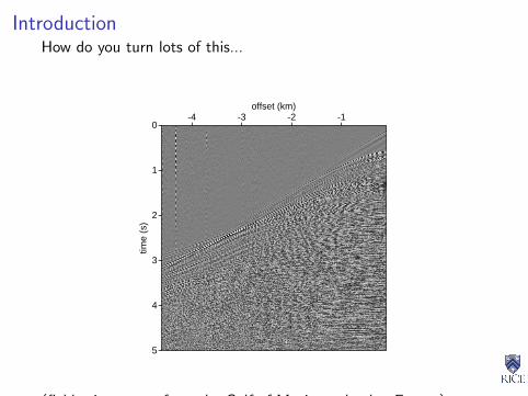
IntroductionHow do you turn lots of this...

0

1

2

3

4

5

time

(s)

-4 -3 -2 -1offset (km)

(field seismogram from the Gulf of Mexico - thanks: Exxon.)

Introductioninto this?

0

500

1000

1500

2000

2500

Dep

th in

Met

ers

0 200 400 600 800 1000 1200 1400CDP

Introduction

Main goal of these lectures: coherent mathematical view ofreflection seismic imaging, as practiced in petroleum industry

I imaging = approximate solution of inverse problem for waveequation

I most practical imaging methods based on linearization(“perturbation theory”)

I high frequency asymptotics (“microlocal analysis”) key tounderstanding

I limitations of linearization lead to many open problems

Lots of mathematics - much yet to be created - with practicalimplications!

AgendaSeismic inverse problem: the sedimentary Earth, reflection seismicmeasurements, the acoustic model, linearization, reflectors andreflections idealized via harmonic analysis of singularities

High frequency asymptotics: why adjoints of modeling operatorsare imaging operators (“Kirchhoff migration”). Beylkin-Rakesh-...theory of high frequency asymptotic inversion

Adjoint state imaging with the wave equation: reverse time andreverse depth

Geometric optics, Rakesh’s construction, and asymptotic inversionw/ caustics and multipathing, imaging artifacts, and prestackmigration apres Claerbout.

A step beyond linearization: a mathematical framework for velocityanalysis

Reflection seismology

aka active source seismology, seismic sounding/profiling

uses acoustic (sound) waves to probe the Earth’s sedimentary crust

main exploration tool of oil & gas industry, also used inenvironmental and civil engineering (hazard detection, bedrockprofiling) and academic geophysics (structure of crust and mantle)

highest resolution imaging technology for deep Earth exploration,in comparison with static (gravimetry, resistivity) or diffusive(active source EM) techniques - works because

waves transfer space-time resolved information from one place toanother with (relatively) little loss

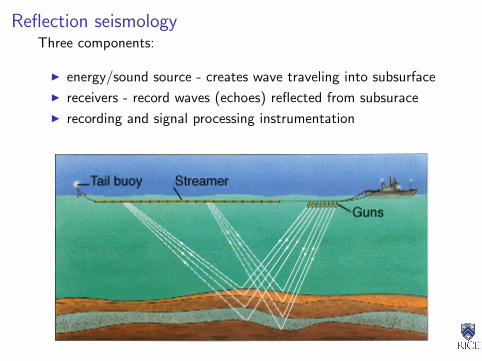
Reflection seismologyThree components:

I energy/sound source - creates wave traveling into subsurface

I receivers - record waves (echoes) reflected from subsurace

I recording and signal processing instrumentation

Reflection seismology

Three components:

I energy/sound source - creates wave traveling into subsurface

I receivers - record waves (echoes) reflected from subsurace

I recording and signal processing instrumentation

Survey consists of many experiments = shots

Each shot = use of one source, localized in time and space -position xs

Simultaneous recording of reflections as many localized receivers,positions xs , time interval = 0− O(10)s after initiation of source.

Reflection seismologyMarine reflection seismology:

I typical energy source: airgun array - releases (array of)supersonically expanding bubbles of compressed air, generatessound pulse in water

I typical receivers: hydrophones (waterproof microphones) inone or more 5-10 km flexible streamer(s) - wired together 500- 30000 groups

I survey ships - lots of recording, processing capacity

hydrophone streameracoustic source(airgun array)x xr sh

Land acquisition similar, but acquisition and processing are morecomplex. Vast bulk (90%+) of data acquired each year is marine.

Reflection seismology

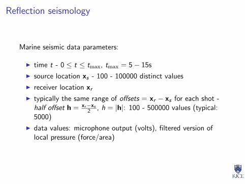
Marine seismic data parameters:

I time t - 0 ≤ t ≤ tmax, tmax = 5− 15s

I source location xs - 100 - 100000 distinct values

I receiver location xr

I typically the same range of offsets = xr − xs for each shot -half offset h = xr−xs

2 , h = |h|: 100 - 500000 values (typical:5000)

I data values: microphone output (volts), filtered version oflocal pressure (force/area)

Reflection seismology

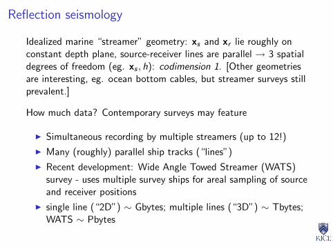
Idealized marine “streamer” geometry: xs and xr lie roughly onconstant depth plane, source-receiver lines are parallel → 3 spatialdegrees of freedom (eg. xs , h): codimension 1. [Other geometriesare interesting, eg. ocean bottom cables, but streamer surveys stillprevalent.]

How much data? Contemporary surveys may feature

I Simultaneous recording by multiple streamers (up to 12!)

I Many (roughly) parallel ship tracks (“lines”)

I Recent development: Wide Angle Towed Streamer (WATS)survey - uses multiple survey ships for areal sampling of sourceand receiver positions

I single line (“2D”) ∼ Gbytes; multiple lines (“3D”) ∼ Tbytes;WATS ∼ Pbytes

Distinguished data subsets

I traces = data for one source, one receiver: t 7→ d(xr , t; xs) -function of t, time series, single channel

I gathers or bins = subsets of traces, extracted from data afteracquisition. Characterized by common value of an acquisitionparameter

Examples:

I shot (or common source) gather: traces w/ same shotlocation xs (previous expls)

I offset (or common offset) gather: traces w/ same half offset h

I ...

Shot gather, Mississippi Canyon

0

1

2

3

4

5

time

(s)

-4 -3 -2 -1offset (km)

(thanks: Exxon)

Shot gather, Mississippi Canyon

1.0

1.5

2.0

2.5

3.0

-2.5 -2.0 -1.5 -1.0 -0.5

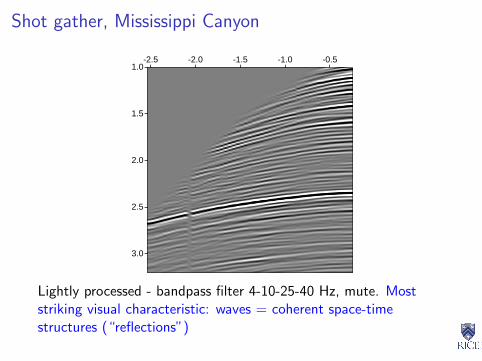
Lightly processed - bandpass filter 4-10-25-40 Hz, mute. Moststriking visual characteristic: waves = coherent space-timestructures (“reflections”)

Shot gather, Mississippi Canyon

1.0

1.5

2.0

2.5

3.0

-2.5 -2.0 -1.5 -1.0 -0.5

What features in the subsurface structure cause reflections? Howto model?

Well logs: a “direct” view of the subsurface

1000 1200 1400 1600 1800 2000 2200 2400 2600 2800 3000500

1000

1500

2000

2500

3000

3500

4000

4500

depth (m)

Blocked logs from well in North Sea (thanks: Mobil R & D). Solid:p-wave velocity (m/s), dashed: s-wave velocity (m/s), dash-dot:density (kg/m3). “Blocked” means “averaged” (over 30 mwindows). Original sample rate of log tool < 1 m.

Well logs: a “direct” view of the subsurface

1000 1200 1400 1600 1800 2000 2200 2400 2600 2800 3000500

1000

1500

2000

2500

3000

3500

4000

4500

depth (m)

You see:

I Trends = slow increase in velocities, density - scale of km

I Reflectors = jumps in velocities, density - scale of m or 10sof m

The Modeling Task

A useful model of the reflection seismology experiment must

I predict wave motion

I produce reflections from reflectors

I accomodate significant variation of wave velocity, materialdensity,...

A really good model will also accomodate

I multiple wave modes, speeds

I material anisotropy

I attenuation, frequency dispersion of waves

I complex source, receiver characteristics

The Acoustic Model

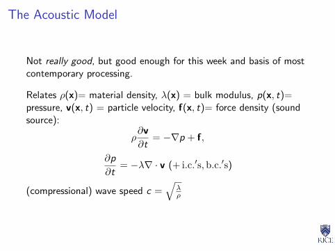
Not really good, but good enough for this week and basis of mostcontemporary processing.

Relates ρ(x)= material density, λ(x) = bulk modulus, p(x, t)=pressure, v(x, t) = particle velocity, f(x, t)= force density (soundsource):

ρ∂v

∂t= −∇p + f,

∂p

∂t= −λ∇ · v (+ i.c.′s,b.c.′s)

(compressional) wave speed c =√

λρ

The Acoustic Model

acoustic field potential u(x, t) =∫ t−∞ ds p(x, s):

p =∂u

∂t, v =

1

ρ∇u

Equivalent form: second order wave equation for potential

1

ρc2

∂2u

∂t2−∇ · 1

ρ∇u =

∫ t

−∞dt∇ ·

(f

ρ

)≡ f

ρ

plus initial, boundary conditions.

The Acoustic Model

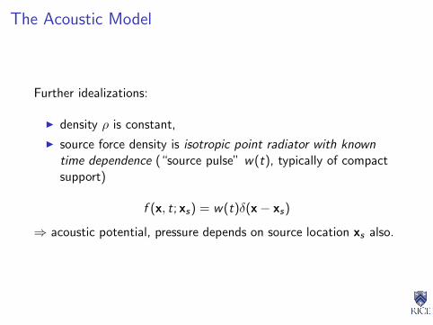
Further idealizations:

I density ρ is constant,

I source force density is isotropic point radiator with knowntime dependence (“source pulse” w(t), typically of compactsupport)

f (x, t; xs) = w(t)δ(x− xs)

⇒ acoustic potential, pressure depends on source location xs also.

Homogeneous acoustics

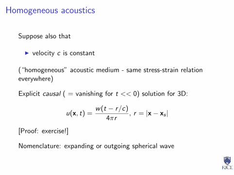
Suppose also that

I velocity c is constant

(“homogeneous” acoustic medium - same stress-strain relationeverywhere)

Explicit causal ( = vanishing for t << 0) solution for 3D:

u(x, t) =w(t − r/c)

4πr, r = |x− xs |

[Proof: exercise!]

Nomenclature: expanding or outgoing spherical wave

Homogeneous acoustics

Also explicit solution (up to quadrature) in 2D - a bit morecomplicated (Poisson’s formula - exercise: find it! eg. in Courantand Hilbert)

Looks like expanding circular wavefront for typical w(t)[SIMULATION]

Observe: no reflections!!! [SIMULATION]

Upshot: if acoustic model is at all appropriate, must usenon-constant c to explain observations.

Natural mathematical question: how nonconstant can c be andstill permit “reasonable” solutions of wave equation?

Heterogeneous acoustics

Weak solution of Dirichlet problem in Ω ⊂ R3 (similar treatmentfor other b. c.’s):

u ∈ C 1([0,T ]; L2(Ω)) ∩ C 0([0,T ]; H10 (Ω))

satisfying for any φ ∈ C∞0 ((0,T )× Ω),∫ T

0

∫Ω

dt dx

1

ρc2

∂u

∂t

∂φ

∂t− 1

ρ∇u · ∇φ+

1

ρf φ

= 0

Theorem (Lions, 1972) Suppose that log ρ, log c ∈ L∞(Ω),f ∈ L2(Ω× R). Then weak solutions of Dirichlet problem exist;initial data

u(·, 0) ∈ H10 (Ω),

∂u

∂t(·, 0) ∈ L2(Ω)

uniquely determine them.

Key Ideas in Proof

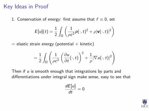
1. Conservation of energy: first assume that f ≡ 0, set

E [u](t) =1

2

∫Ω

(1

ρc2p(·, t)2 + ρ|v(·, t)|2

)= elastic strain energy (potential + kinetic)

=1

2

∫Ω

(1

ρc2

(∂u

∂t(·, t)

)2

+1

ρ|∇u(·, t)|2

)

Then if u is smooth enough that integrations by parts anddifferentiations under integral sign make sense, easy to see that

dE [u]

dt= 0

Key Ideas in Proof

General case (f 6= 0): with help of Cauchy-Schwarz ≤,

dE [u]

dt(t) ≤ const.

(E [u](t) +

∫ t

0ds

∫Ω

dx f 2(x, s)

)whence for 0 ≤ t ≤ T ,

E [u](t) ≤ const.(

E [u](0) +

∫ t

0ds

∫Ω

dx f 2(x, s)

)(Gronwall’s ≤)

const on RHS bounded by T , ‖ log ρ‖L∞(Ω), ‖ log c‖L∞(Ω)

Key Ideas in Proof

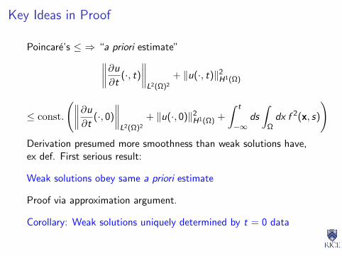
Poincare’s ≤ ⇒ “a priori estimate”∥∥∥∥∂u

∂t(·, t)

∥∥∥∥L2(Ω)2

+ ‖u(·, t)‖2H1(Ω)

≤ const.

(∥∥∥∥∂u

∂t(·, 0)

∥∥∥∥L2(Ω)2

+ ‖u(·, 0)‖2H1(Ω) +

∫ t

−∞ds

∫Ω

dx f 2(x, s)

)Derivation presumed more smoothness than weak solutions have,ex def. First serious result:

Weak solutions obey same a priori estimate

Proof via approximation argument.

Corollary: Weak solutions uniquely determined by t = 0 data

Key Ideas in Proof

2. Galerkin approximation: Pick increasing sequence of subspaces

W 0 ⊂W 1 ⊂W 2 ⊂ ... ⊂ H10 (Ω)

so that∪∞n=0W n dense in L2(Ω)

Typical example: piecewise linear Finite Element subspaces onsequence of meshes, each refinement of preceding.

Galerkin principle: find un ∈ C 2([0,T ],W n) so that for anyφn ∈ C 1([0,T ],W n),∫ T

0

∫Ω

dt dx

1

ρc2

∂un

∂t

∂φn

∂t− 1

ρ∇un · ∇φn +

1

ρf φn

= 0

Key Ideas in Proof

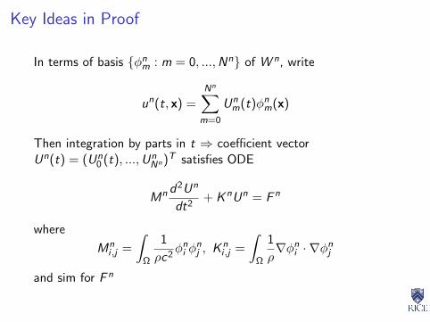
In terms of basis φnm : m = 0, ...,Nn of W n, write

un(t, x) =Nn∑

m=0

Unm(t)φn

m(x)

Then integration by parts in t ⇒ coefficient vectorUn(t) = (Un

0 (t), ...,UnNn)T satisfies ODE

Mn d2Un

dt2+ KnUn = F n

where

Mni ,j =

∫Ω

1

ρc2φn

i φnj , Kn

i ,j =

∫Ω

1

ρ∇φn

i · ∇φnj

and sim for F n

Key Ideas in Proof

Assume temporarily that f ∈ C 0([0,T ], L2(Ω)) ⊂ L2([0,T ]× Ω) -then F n ∈ C 0([0,T ],W n), so...

basic theorem on ODEs ⇒ existence of Galerkin approximation un.

Energy estimate for Galerkin approximation -

E [un](t) ≤ const.(

E [un](0) +

∫ t

0‖f (·, t)‖2

L2(Ω)

)constant independent of n.

Alaoglu Thm ⇒ un weakly precompact in L2([0,T ],H10 (Ω)),

∂un/∂t weakly precompact in L2([0,T ], L2(Ω)), so can selectweakly convergent sequence, limit u ∈ L2([0,T ],H1

0 (Ω)),∂u/∂t ∈ L2([0,T ], L2(Ω)).

Key Ideas in Proof

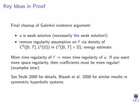
Final cleanup of Galerkin existence argument:

I u is weak solution (necessarily the weak solution!)

I remove regularity assumption on f via density ofC 0([0,T ], L2(Ω)) in L2([0,T ]× Ω), energy estimate

More time regularity of f ⇒ more time regularity of u. If you wantmore space regularity, then coefficients must be more regular!(examples later)

See Stolk 2000 for details, Blazek et al. 2008 for similar results resymmetric hyperbolic systems

Reflection seismic inverse problem

Forward map S = time history of pressure for each sourcelocation xs at receiver locations xr , as function of c

Reality: xs samples finitely many points near surface of Earth(z = 0), active receiver locations xr may depend on sourcelocations and are also discrete

but: sampling is reasonably fine (see plots!) so...

Idealization: (xs , xr ) range over 4-diml closed submfd withboundary Σ, source and receiver depths constant.

Reflection seismic inverse problem

(predicted seismic data), depends on velocity field c(x):

F [c] = p|Σ×[0,T ]

Inverse problem: given observed seismic data d ∈ L2(Σ× [0,T ]),find c so that

F [c] ' d

This inverse problem is

I large scale - Tbytes of data, Pflops to simulate forward map

I nonlinear

I yields to no known direct attack (no “solution formula”)

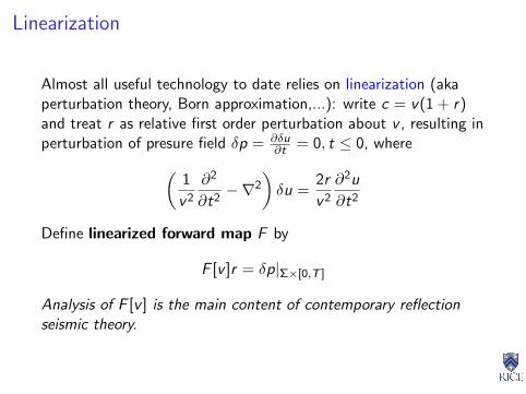
Linearization

Almost all useful technology to date relies on linearization (akaperturbation theory, Born approximation,...): write c = v(1 + r)and treat r as relative first order perturbation about v , resulting inperturbation of presure field δp = ∂δu

∂t = 0, t ≤ 0, where(1

v 2

∂2

∂t2−∇2

)δu =

2r

v 2

∂2u

∂t2

Define linearized forward map F by

F [v ]r = δp|Σ×[0,T ]

Analysis of F [v ] is the main content of contemporary reflectionseismic theory.

Linearization in theory

Recall Lions-Stolk result: if log c ∈ L∞(Ω) (ρ = 1!) andf ∈ L2(Ω× [0,T ]), then weak solution has finite energy, i.e.

u = u[c] ∈ C 1([0,T ], L2(Ω)) ∩ C 0([0,T ],H10 (Ω))

Suppose δc ∈ L∞(Ω), define δu by solving perturbational problem:set v = c , r = δc/c .

Linearization in theory

Stolk (2000): for small enough h ∈ R,

‖u[c + hδc]− u[c]− δu‖C0([0,T ],L2(Ω)) = o(h)

Note “loss of derivative”: error in Newton quotient is o(1) inweaker norm than that of space of weak solns

Implication for F [c]: under suitable circumstances (c = const.near Σ - “marine” case),

‖F [c]‖L2(Σ×[0,T ]) = O(‖w‖L2(R))

but

‖F [v(1 + r)]−F [v ]− F [v ]r‖L2(Σ×[0,T ]) = O(‖w‖H1(R))

and these estimates are both sharp

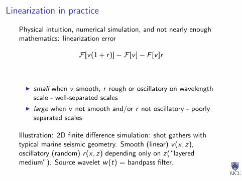
Linearization in practice

Physical intuition, numerical simulation, and not nearly enoughmathematics: linearization error

F [v(1 + r)]−F [v ]− F [v ]r

I small when v smooth, r rough or oscillatory on wavelengthscale - well-separated scales

I large when v not smooth and/or r not oscillatory - poorlyseparated scales

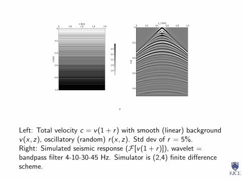
Illustration: 2D finite difference simulation: shot gathers withtypical marine seismic geometry. Smooth (linear) v(x , z),oscillatory (random) r(x , z) depending only on z(“layeredmedium”). Source wavelet w(t) = bandpass filter.

0

0.2

0.4

0.6

0.8

1.0

z (k

m)

0 0.5 1.0 1.5 2.0x (km)

1.6

1.8

2.0

2.2

2.4

,

0

0.2

0.4

0.6

0.8

t (s)

0 0.2 0.4 0.6 0.8 1.0x_r (km)

Left: Total velocity c = v(1 + r) with smooth (linear) backgroundv(x , z), oscillatory (random) r(x , z). Std dev of r = 5%.Right: Simulated seismic response (F [v(1 + r)]), wavelet =bandpass filter 4-10-30-45 Hz. Simulator is (2,4) finite differencescheme.

0

0.2

0.4

0.6

0.8

1.0

z (k

m)

0 0.5 1.0 1.5 2.0x (km)

1.6

1.8

2.0

2.2

2.4

,

0

0.2

0.4

0.6

0.8

1.0

z (k

m)

0 0.5 1.0 1.5 2.0x (km)

-0.10

-0.05

0

0.05

0.10

Decomposition of model in previous slide as smooth background(left, v(x , z)) plus rough perturbation (right, r(x , z)).

0

0.2

0.4

0.6

0.8

t (s)

0 0.2 0.4 0.6 0.8 1.0x_r (km)

.

0

0.2

0.4

0.6

0.8

t (s)

0 0.2 0.4 0.6 0.8 1.0x_r (km)

Left: Simulated seismic response of smooth model (F [v ]),Right: Simulated linearized response, rough perturbation ofsmooth model (F [v ]r)

0

0.2

0.4

0.6

0.8

t (s)

0 0.2 0.4 0.6 0.8 1.0x_r (km)

.

0

0.2

0.4

0.6

0.8

t (s)

0 0.2 0.4 0.6 0.8 1.0x_r (km)

Left: Simulated seismic response of rough model (F [0.95v + r ]),Right: Simulated linearized response, smooth perturbation ofrough model (F [0.95v + r ]((0.05v)/(0.95v + r)))

0

0.2

0.4

0.6

0.8

t (s)

0 0.2 0.4 0.6 0.8 1.0x_r (km)

,

0

0.2

0.4

0.6

0.8

t (s)

0 0.2 0.4 0.6 0.8 1.0x_r (km)

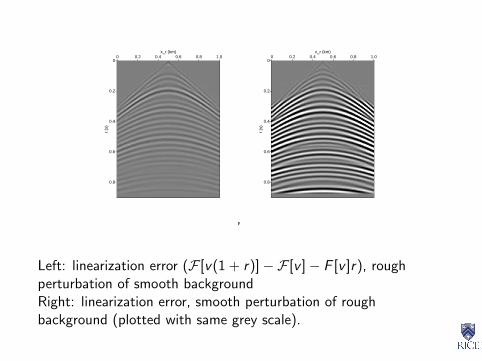
Left: linearization error (F [v(1 + r)]−F [v ]− F [v ]r), roughperturbation of smooth backgroundRight: linearization error, smooth perturbation of roughbackground (plotted with same grey scale).

Summary

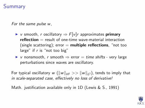
For the same pulse w ,

I v smooth, r oscillatory ⇒ F [v ]r approximates primaryreflection = result of one-time wave-material interaction(single scattering); error = multiple reflections, “not toolarge” if r is “not too big”

I v nonsmooth, r smooth ⇒ error = time shifts - very largeperturbations since waves are oscillatory.

For typical oscillatory w (‖w‖H1 >> ‖w‖L2), tends to imply thatin scale-separated case, effectively no loss of derivative!

Math. justification available only in 1D (Lewis & S., 1991)

Velocity Analysis and Imaging

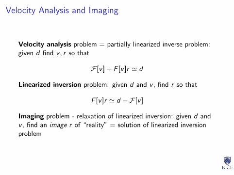
Velocity analysis problem = partially linearized inverse problem:given d find v , r so that

F [v ] + F [v ]r ' d

Linearized inversion problem: given d and v , find r so that

F [v ]r ' d −F [v ]

Imaging problem - relaxation of linearized inversion: given d andv , find an image r of “reality” = solution of linearized inversionproblem

Velocity Analysis and Imaging

Last 20 years:

I much progress on imaging

I lots of progress on linearized inversion

I much less on velocity analysis

Interesting question: what’s an image?

“...I know it when I see it.” - Associate Justice PotterStewart, 1964

Aymptotic assumption

Linearization is accurate ⇔ length scale of v >> length scale ofr ' wavelength, properties of F [v ] dominated by those of Fδ[v ] (=F [v ] with w = δ). Implicit in migration concept (eg. Hagedoorn,1954); explicit use: Cohen & Bleistein, SIAM JAM 1977.

Key idea: reflectors (rapid changes in r) emulate singularities;reflections (rapidly oscillating features in data) also emulatesingularities.

NB: “everybody’s favorite reflector”: the smooth interface acrosswhich r jumps. But this is an oversimplification - reflectors in theEarth may be complex zones of rapid change, pehaps in alldirections. More flexible notion needed!!

Wave Front Sets

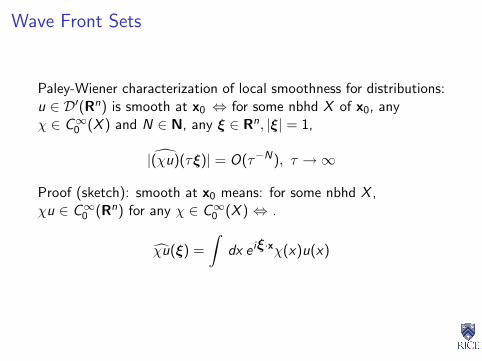
Paley-Wiener characterization of local smoothness for distributions:u ∈ D′(Rn) is smooth at x0 ⇔ for some nbhd X of x0, anyχ ∈ C∞0 (X ) and N ∈ N, any ξ ∈ Rn, |ξ| = 1,

|(χu)(τξ)| = O(τ−N), τ →∞

Proof (sketch): smooth at x0 means: for some nbhd X ,χu ∈ C∞0 (Rn) for any χ ∈ C∞0 (X ) ⇔ .

χu(ξ) =

∫dx e iξ·xχ(x)u(x)

Wave Front Sets

=

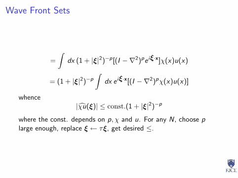
∫dx (1 + |ξ|2)−p[(I −∇2)pe iξ·x]χ(x)u(x)

= (1 + |ξ|2)−p

∫dx e iξ·x[(I −∇2)pχ(x)u(x)]

whence|χu(ξ)| ≤ const.(1 + |ξ|2)−p

where the const. depends on p, χ and u. For any N, choose plarge enough, replace ξ ← τξ, get desired ≤.

Wave Front Sets

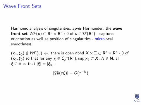
Harmonic analysis of singularities, apres Hormander: the wavefront set WF (u) ⊂ Rn × Rn \ 0 of u ∈ D′(Rn) - capturesorientation as well as position of singularities - microlocalsmoothness

(x0, ξ0) /∈WF (u) ⇔, there is open nbhd X × Ξ ⊂ Rn × Rn \ 0 of(x0, ξ0) so that for any χ ∈ C∞0 (Rn), suppχ ⊂ X , N ∈ N, allξ ∈ Ξ so that |ξ| = |ξ0|,

|χu(τξ)| = O(τ−N)

Housekeeping chores

(i) note that the nbhds Ξ may naturally be taken to be cones

(ii) WF (u) is invariant under chg. of coords if it is regarded as asubset of the cotangent bundle T ∗(Rn) (i.e. the ξ componentstransform as covectors).

(iii) The standard example: if u jumps across the interfaceφ(x) = 0, otherwise smooth, thenWF (u) ⊂ Nφ = (x, ξ) : φ(x) = 0, ξ||∇φ(x) (normal bundle ofφ = 0)

[Good refs for basics on WF: Duistermaat, 1996; Taylor, 1981;Hormander, 1983]

Housekeeping chores

Proof of (ii): follows from

(iv) Basic estimate for oscillatory integrals: suppose thatψ ∈ C∞(Rn),∇ψ(x0) 6= 0, (x0,∇ψ(x0)) /∈WF (u). Then for anyχ ∈ C∞0 (Rn) supported in small enough nbhd of x0, and anyN ∈ N, ∫

dx e iτψ(x)χ(x)u(x) = O(τ−N)

Housekeeping chores

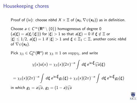
Proof of (iv): choose nbhd X × Ξ of (x0,∇ψ(x0)) as in definition.

Choose a ∈ C∞(Rn \ 0) homogeneous of degree 0(a(ξ) = a(ξ/|ξ|)) for |ξ| > 1 so that a(ξ) = 0 if ξ /∈ Ξ or|ξ| ≤ 1/2, a(ξ) = 1 if |ξ| > 1 and ξ ∈ Ξ1 ⊂ Ξ, another conic nbhdof ∇ψ(x0).

Pick χ1 ∈ C∞0 (Rn) st χ1 ≡ 1 on suppχ, and write

χ(x)u(x) = χ1(x)(2π)−n

∫dξ e ix·ξχu(ξ)

= χ1(x)(2π)−n

∫dξ e ix·ξg1(ξ) + χ1(x)(2π)−n

∫dξ e ix·ξg2(ξ)

in which g1 = aχu, g2 = (1− a)χu

Housekeeping chores

So∫dx e iτψ(x)χ(x)u(x) =

∑j=1,2

∫dx

∫dξ e i(τψ(x)+x·ξ)χ1(x)gj(ξ)

For ξ ∈ supp(1− a) (excludes a conic nbhd of ∇ψ(x0)), can write

e i(τψ(x)+x·ξ) = [−i |τ∇ψ(x) + ξ|−2(τ∇ψ(x) + ξ) · ∇]pe i(τψ(x)+x·ξ)

Can guarantee that |τ∇ψ(x) + ξ| > 0 by choosing suppχ1 suff.small, so that in dom. of integration ∇ψ(x) is close to ∇ψ(x0). Infact, for ξ ∈ supp(1− a), suppχ1 small enough, and x ∈ suppχ1,

|τ∇ψ(x) + ξ| > Cτ

for some C > 0. Exercise: prove this!

Housekeeping choresSubstitute and integrate by parts, use above estimate to get∣∣∣∣∫ dx

∫dξ e i(τψ(x)+x·ξ)χ1(x)g2(ξ)

∣∣∣∣ ≤ const.τ−N

for any N.

Note that for ξ ∈ suppa,

|χu(ξ)| ≤ const.|ξ|−p

for any p (with p-dep. const, of course!). Follows that

h(bx) =

∫dξ e ix·ξg1(ξ)

converges absolutely, also after differentiating any number of timesunder the integral sign, therefore h ∈ C∞(Rn), whence∫

dx

∫dξ e i(τψ(x)+x·ξ)χ1(x)g1(ξ) =

∫dx e iτψ(x)χ1(x)h(x)

Housekeeping chores

with integrand supported as near as you like to x0. Since∇ψ(x0) 6= 0, same is true of suppχ1 provided this is chosen smallenough; now use

e iτψ(x) = τ−p(−i |∇ψ(x)|−2∇ψ(x) · ∇)pe iτψ(x)

and integration by parts again to show that this term is alsoO(τ−N) any N.

Housekeeping chores

Proof of (ii), for u integrable (Exercise: formulate and provesimilar statement for distributions)

Equivalent statement: suppose that F : U → Rn is adiffeomorphism on an open U ⊂ Rn, suppu ⊂ F (U), x0 ∈ U,y0 = F (x0), and (y0, η0) /∈WF (u).

Claim: then (x0, ξ0) /∈WF (u F ), where ξ0 = DF (x0)Tη0.

Housekeeping chores

Need to show that if χ ∈ C∞0 (Rn), x0 ∈ suppχ and small enough,

then χu F (τξ) = O(τ−N) any N for ξ conically near ξ0. Fromthe change-of-variables formula

χu F (τξ) =

∫dxχ(x)(u F )(x)e iτx·ξ

=

∫dy (χ F−1)(y)u(y)e iτξ·F−1(y) det D(F−1)(y)

Set j = χ F−1detD(F−1). Note: j ∈ C∞0 (Rn) supported in nbhdV of y0 if χ supported in F−1(V).

Housekeeping chores

MVT: for y close enough to y0,

F−1(y) = x0 +

∫ 1

0dσDF−1(y0 + σ(y − y0))(y − y0)

Insert in exponent to get

χu F (τξ) = e iτx0·ξ∫

dy j(y)u(y)eiτψξ(y)

where

ψξ(y) = (y − y0) ·∫ 1

0dσDF−1(y0 + σ(y − y0))Tξ

Since∇ψξ(y0) = DF−1(y0)ξ

claim now follows from basic thm on oscillatory integrals.

Housekeeping chores

Proof of (iii): Function of compact supp, jumping across φ = 0

u = χH(φ)

with χ smooth, H = Heaviside function (H(t) = 1, t > 0 andH(t) = 0, t < 0).

Pick x0 with φ(x0) = 0. Surface φ = 0 regular near x0 if∇φ(x0) 6= 0 - assume this.

Suffices to consider case of χ ∈ C∞0 (Rn) of small support cont’gx0. Inverse Function Thm ⇒ exists diffeo F mapping nbhd of x0

to nbhd of 0 so that F (x0) = 0 and F1(x) = φ(x). Fact (ii) ⇒reduce to case φ(x) = x1 - Exercise: do this!

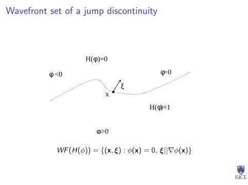
Wavefront set of a jump discontinuity

H(

)=0

φ

φ

=0φ

φ)=1

>0

<0

φH(

ξx

WF (H(φ)) = (x, ξ) : φ(x) = 0, ξ||∇φ(x)

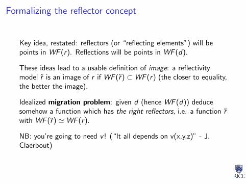
Formalizing the reflector concept

Key idea, restated: reflectors (or “reflecting elements”) will bepoints in WF (r). Reflections will be points in WF (d).

These ideas lead to a usable definition of image: a reflectivitymodel r is an image of r if WF (r) ⊂WF (r) (the closer to equality,the better the image).

Idealized migration problem: given d (hence WF (d)) deducesomehow a function which has the right reflectors, i.e. a function rwith WF (r) 'WF (r).

NB: you’re going to need v ! (“It all depends on v(x,y,z)” - J.Claerbout)

AgendaSeismic inverse problem: the sedimentary Earth, reflection seismicmeasurements, the acoustic model, linearization, reflectors andreflections idealized via harmonic analysis of singularities

High frequency asymptotics: why adjoints of modeling operatorsare imaging operators (“Kirchhoff migration”). Beylkin-Rakesh-...theory of high frequency asymptotic inversion

Adjoint state imaging with the wave equation: reverse time andreverse depth

Geometric optics, Rakesh’s construction, and asymptotic inversionw/ caustics and multipathing, imaging artifacts, and prestackmigration apres Claerbout.

A step beyond linearization: a mathematical framework for velocityanalysis

Microlocal property of differential operators

Suppose u ∈ D′(Rn), (x0, ξ0) /∈WF (u), and P(x,D) is a partialdifferential operator:

P(x,D) =∑|α|≤m

aα(x)Dα

D = (D1, ...,Dn), Di = −i∂

∂xi

α = (α1, ..., αn), |α| =∑

i

αi ,

Dα = Dα11 ...Dαn

n

Then (x0, ξ0) /∈WF (P(x,D)u) [i.e.: WF (Pu) ⊂WF (u)].

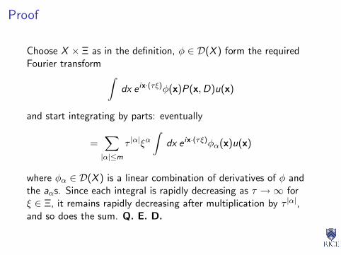
Proof

Choose X × Ξ as in the definition, φ ∈ D(X ) form the requiredFourier transform ∫

dx e ix·(τξ)φ(x)P(x,D)u(x)

and start integrating by parts: eventually

=∑|α|≤m

τ |α|ξα∫

dx e ix·(τξ)φα(x)u(x)

where φα ∈ D(X ) is a linear combination of derivatives of φ andthe aαs. Since each integral is rapidly decreasing as τ →∞ forξ ∈ Ξ, it remains rapidly decreasing after multiplication by τ |α|,and so does the sum. Q. E. D.

Integral representation of linearized operator

With w = δ, acoustic potential u is same as Causal Green’sfunction G (x, t; xs) = retarded fundamental solution:(

1

v 2

∂2

∂t2−∇2

)G (x, t; xs) = δ(t)δ(x− xs)

and G ≡ 0, t < 0. Then (w = δ!) p = ∂G∂t , δp = ∂δG

∂t , and(1

v 2

∂2

∂t2−∇2

)δG (x, t; xs) =

2

v 2(x)

∂2G

∂t2(x, t; xs)r(x)

Simplification: from now on, define F [v ]r = δG |x=xr- i.e. lose a

t-derivative. Duhamel’s principle ⇒

δG (xr , t; xs) =

∫dx

2r(x)

v(x)2

∫ds G (xr , t − s; x)

∂2G

∂t2(x, s; xs)

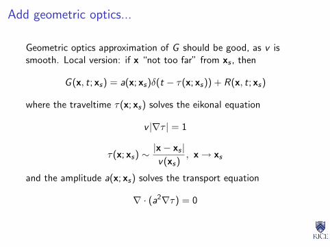
Add geometric optics...

Geometric optics approximation of G should be good, as v issmooth. Local version: if x “not too far” from xs , then

G (x, t; xs) = a(x; xs)δ(t − τ(x; xs)) + R(x, t; xs)

where the traveltime τ(x; xs) solves the eikonal equation

v |∇τ | = 1

τ(x; xs) ∼ |x− xs |v(xs)

, x→ xs

and the amplitude a(x; xs) solves the transport equation

∇ · (a2∇τ) = 0

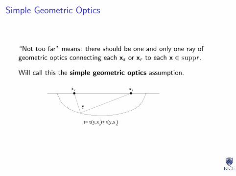
Simple Geometric Optics

“Not too far” means: there should be one and only one ray ofgeometric optics connecting each xs or xr to each x ∈ suppr .

Will call this the simple geometric optics assumption.

(y,x )+ (y,x )ττt=

x x

y

s

r s

r

An oft-forgotten detail

All of this is meaningful only if the remainder R is small in asuitable sense: energy estimate (Exercise!) ⇒

∫dx

∫ T

0dt |R(x, t; xs)|2 ≤ C‖v‖C4

Numerics, and a caution

Numerical solution of eikonal, transport: ray tracing (Lagrangian),various sorts of upwind finite difference (Eulerian) methods. Seeeg. Sethian book, WWS 1999 MGSS notes (online) for details.

For “random but smooth” v(x) with variance σ, more than oneconnecting ray occurs as soon as the distance is O(σ−2/3). Suchmultipathing is invariably accompanied by the formation of acaustic (White, 1982).

Upon caustic formation, the simple geometric optics fielddescription above is no longer correct (Ludwig, 1966).

A caustic example (1)

0 0.1 0.2 0.3 0.4 0.5 0.6 0.7 0.8 0.9 1

0

0.2

0.4

0.6

0.8

1

1.2

1.4

1.6

1.8

2

sin1: velocity field

2D Example of strong refraction: Sinusoidal velocity fieldv(x , z) = 1 + 0.2 sin πz

2 sin 3πx

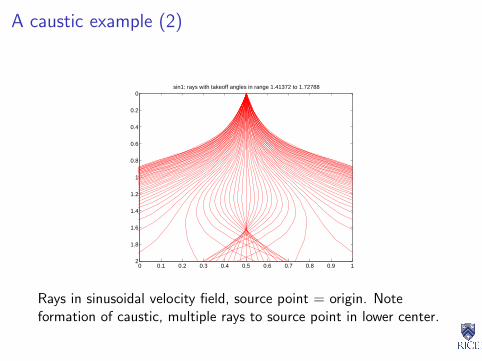
A caustic example (2)

0 0.1 0.2 0.3 0.4 0.5 0.6 0.7 0.8 0.9 1

0

0.2

0.4

0.6

0.8

1

1.2

1.4

1.6

1.8

2

sin1: rays with takeoff angles in range 1.41372 to 1.72788

Rays in sinusoidal velocity field, source point = origin. Noteformation of caustic, multiple rays to source point in lower center.

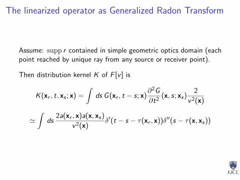
The linearized operator as Generalized Radon Transform

Assume: supp r contained in simple geometric optics domain (eachpoint reached by unique ray from any source or receiver point).

Then distribution kernel K of F [v ] is

K (xr , t, xs ; x) =

∫ds G (xr , t − s; x)

∂2G

∂t2(x, s; xs)

2

v 2(x)

'∫

ds2a(xr , x)a(x, xs)

v 2(x)δ′(t − s − τ(xr , x))δ′′(s − τ(x, xs))

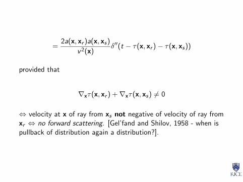
=2a(x, xr )a(x, xs)

v 2(x)δ′′(t − τ(x, xr )− τ(x, xs))

provided that

∇xτ(x, xr ) +∇xτ(x, xs) 6= 0

⇔ velocity at x of ray from xs not negative of velocity of ray fromxr ⇔ no forward scattering. [Gel’fand and Shilov, 1958 - when ispullback of distribution again a distribution?].

Q: What does ' mean?

A: It means “differs by something smoother”.

In theory, can complete the geometric optics approximation of theGreen’s function so that the difference is C∞ - then the two sideshave the same singularities, ie. the same wavefront set.

In practice, it’s sufficient to make the difference just a bitsmoother, so the first term of the geometric optics approximation(displayed above) suffices (can formalize this with modification ofwavefront set defn).

These lectures will ignore the distinction.

GRT = “Kirchhoff” modeling

So: for r supported in simple geometric optics domain, no forwardscattering ⇒

δG (xr , t; xs) '

∂2

∂t2

∫dx

2r(x)

v 2(x)a(x, xr )a(x, xs)δ(t − τ(x, xr )− τ(x, xs))

That is: pressure perturbation is sum (integral) of r over reflectionisochron x : t = τ(x, xr ) + τ(x, xs), w. weighting, filtering. Note:if v =const. then isochron is ellipsoid, as τ(xs , x) = |xs − x|/v !

(y,x )+ (y,x )ττt=

x x

y

s

r s

r

Zero Offset data and the Exploding Reflector

Zero offset data (xs = xr ) is seldom actually measured (contrastradar, sonar!), but routinely approximated through NMO-stack (tobe explained later).

Extracting image from zero offset data, rather than from all(100’s) of offsets, is tremendous data reduction - whenapproximation is accurate, leads to excellent images.

Imaging basis: the exploding reflector model (Claerbout, 1970’s).

For zero-offset data, distribution kernel of F [v ] is

K (xs , t, xs ; x) =∂2

∂t2

∫ds

2

v 2(x)G (xs , t − s; x)G (x, s; xs)

Under some circumstances (explained below), K ( = Gtime-convolved with itself) is “similar” (also explained) to G =Green’s function for v/2. Then

δG (xs , t; xs) ∼ ∂2

∂t2

∫dx G (xs , t, x)

2r(x)

v 2(x)

∼ solution w of (4

v 2

∂2

∂t2−∇2

)w = δ(t)

2r

v 2

Thus reflector “explodes” at time zero, resulting field propagates in“material” with velocity v/2.

Explain when the exploding reflector model “works”, i.e. when Gtime-convolved with itself is “similar” to G = Green’s function forv/2. If supp r lies in simple geometry domain, then

K (xs , t, xs ; x) =

∫ds

2a2(x, xs)

v 2(x)δ(t − s − τ(xs , x))δ′′(s − τ(x, xs))

=2a2(x, xs)

v 2(x)δ′′(t − 2τ(x, xs))

whereas the Green’s function G for v/2 is

G (x, t; xs) = a(x, xs)δ(t − 2τ(x, xs))

(half velocity = double traveltime, same rays!).

Difference between effects of K , G : for each xs scale r by smoothfcn - preserves WF (r) hence WF (F [v ]r) and relation betweenthem. Also: adjoints have same effect on WF sets.

Upshot: from imaging point of view (i.e. apart from amplitude,derivative (filter)), kernel of F [v ] restricted to zero offset is sameas Green’s function for v/2, provided that simple geometryhypothesis holds: only one ray connects each source point to eachscattering point, ie. no multipathing.

See Claerbout, IEI, for examples which demonstrate thatmultipathing really does invalidate exploding reflector model.

Standard Processing

Inspirational interlude: the sort-of-layered theory =“StandardProcessing”

Suppose were v ,r functions of z = x3 only, all sources andreceivers at z = 0. Then the entire system is translation-invariantin x1, x2 ⇒ Green’s function G its perturbation δG , and theidealized data δG |z=0 are really only functions of t and half-offseth = |xs − xr |/2. There would be only one seismic experiment,equivalent to any common midpoint gather (“CMP”).

This isn’t really true - look at the data!!! However it isapproximately correct in many places in the world: CMPs changevery slowly with midpoint xm = (xr + xs)/2.

Standard processing: treat each CMP as if it were the result of anexperiment performed over a layered medium, but permit the layersto vary with midpoint.

Thus v = v(z), r = r(z) for purposes of analysis, but at the endv = v(xm, z), r = r(xm, z).

F [v ]r(xr , t; xs)

'∫

dx2r(z)

v 2(z)a(x, xr )a(x, xs)δ′′(t − τ(x, xr )− τ(x, xs))

=

∫dz

2r(z)

v 2(z)

∫dω

∫dxω2a(x, xr )a(x, xs)e iω(t−τ(x,xr )−τ(x,xs))

Since we have already thrown away smoother (lower frequency)terms, do it again using stationary phase. Upshot (see 2000 MGSSnotes for details): up to smoother (lower frequency) error,

F [v ]r(h, t) ' A(z(h, t), h)R(z(h, t))

Here z(h, t) is the inverse of the 2-way traveltime

t(h, z) = 2τ((h, 0, z), (0, 0, 0))

i.e. z(t(h, z ′), h) = z ′. R is (yet another version of) “reflectivity”

R(z) =1

2

dr

dz(z)

That is, F [v ] is a a derivative followed by a change of variablefollowed by multiplication by a smooth function. Substitute t0

(vertical travel time) for z (depth) and you get “Inverse NMO”(t0 → (t, h)). Will be sloppy and call z → (t, h) INMO.

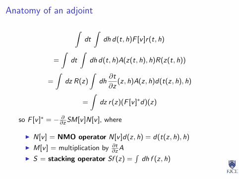
Anatomy of an adjoint

∫dt

∫dh d(t, h)F [v ]r(t, h)

=

∫dt

∫dh d(t, h)A(z(t, h), h)R(z(t, h))

=

∫dz R(z)

∫dh

∂t

∂z(z , h)A(z , h)d(t(z , h), h)

=

∫dz r(z)(F [v ]∗d)(z)

so F [v ]∗ = − ∂∂z SM[v ]N[v ], where

I N[v ] = NMO operator N[v ]d(z , h) = d(t(z , h), h)

I M[v ] = multiplication by ∂t∂z A

I S = stacking operator Sf (z) =∫

dh f (z , h)

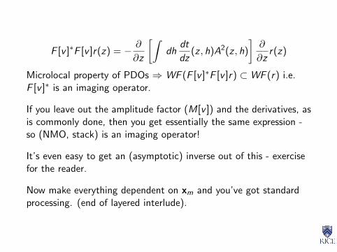
F [v ]∗F [v ]r(z) = − ∂

∂z

[∫dh

dt

dz(z , h)A2(z , h)

]∂

∂zr(z)

Microlocal property of PDOs ⇒ WF (F [v ]∗F [v ]r) ⊂WF (r) i.e.F [v ]∗ is an imaging operator.

If you leave out the amplitude factor (M[v ]) and the derivatives, asis commonly done, then you get essentially the same expression -so (NMO, stack) is an imaging operator!

It’s even easy to get an (asymptotic) inverse out of this - exercisefor the reader.

Now make everything dependent on xm and you’ve got standardprocessing. (end of layered interlude).

Multioffset (“Prestack”) Imaging, apres Beylkin

If d = F [v ]r , thenF [v ]∗d = F [v ]∗F [v ]r

In the layered case, F [v ]∗F [v ] is an operator which preserves wavefront sets. Whenever F [v ]∗F [v ] preserves wave front sets, F [v ]∗ isan imaging operator.

Beylkin, JMP 1985: for r supported in simple geometric opticsdomain,

I WF (Fδ[v ]∗Fδ[v ]r) ⊂WF (r)

I if Sobs = S [v ] + Fδ[v ]r (data consistent with linearizedmodel), then Fδ[v ]∗(Sobs − S [v ]) is an image of r

I an operator Fδ[v ]† exists for which Fδ[v ]†(Sobs − S [v ])− r issmoother than r , under some constraints on r - an inversemodulo smoothing operators or parametrix.

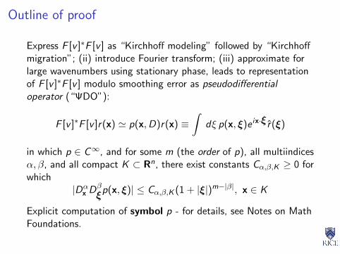
Outline of proof

Express F [v ]∗F [v ] as “Kirchhoff modeling” followed by “Kirchhoffmigration”; (ii) introduce Fourier transform; (iii) approximate forlarge wavenumbers using stationary phase, leads to representationof F [v ]∗F [v ] modulo smoothing error as pseudodifferentialoperator (“ΨDO”):

F [v ]∗F [v ]r(x) ' p(x,D)r(x) ≡∫

dξ p(x, ξ)e ix·ξ r(ξ)

in which p ∈ C∞, and for some m (the order of p), all multiindicesα, β, and all compact K ⊂ Rn, there exist constants Cα,β,K ≥ 0 forwhich

|Dαx Dβ

ξp(x, ξ)| ≤ Cα,β,K (1 + |ξ|)m−|β|, x ∈ K

Explicit computation of symbol p - for details, see Notes on MathFoundations.

Microlocal Propertyof ΨDOs

if p(x ,D) is a ΨDO, u ∈ E ′(Rn) thenWF (p(x ,D)u) ⊂WF (u).

Will prove this, from which imaging property of prestack Kirchhoffmigration follows. First, a few other properties:

I differential operators are ΨDOs (easy - exercise)

I ΨDOs of order m form a module over C∞(Rn) (also easy)

I product of ΨDO order m, ΨDO order l = ΨDO order ≤ m + l ;adjoint of ΨDO order m is ΨDO order m (much harder)

Complete accounts of theory, many apps: books of Duistermaat,Taylor, Nirenberg, Treves, Hormander.

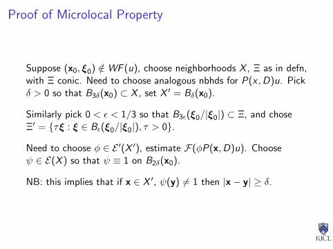
Proof of Microlocal Property

Suppose (x0, ξ0) /∈WF (u), choose neighborhoods X , Ξ as in defn,with Ξ conic. Need to choose analogous nbhds for P(x ,D)u. Pickδ > 0 so that B3δ(x0) ⊂ X , set X ′ = Bδ(x0).

Similarly pick 0 < ε < 1/3 so that B3ε(ξ0/|ξ0|) ⊂ Ξ, and choseΞ′ = τξ : ξ ∈ Bε(ξ0/|ξ0|), τ > 0.

Need to choose φ ∈ E ′(X ′), estimate F(φP(x,D)u). Chooseψ ∈ E(X ) so that ψ ≡ 1 on B2δ(x0).

NB: this implies that if x ∈ X ′, ψ(y) 6= 1 then |x− y| ≥ δ.

Write u = (1− ψ)u + ψu. Claim: φP(x,D)((1− ψ)u) is smooth.

φ(x)P(x,D)((1− ψ)u))(x)

= φ(x)

∫dξ P(x, ξ)e ix·ξ

∫dy (1− ψ(y))u(y)e−iy·ξ

=

∫dξ

∫dy P(x, ξ)φ(x)(1− ψ(y))e i(x−y)·ξu(y)

=

∫dξ

∫dy (−∇2

ξ)MP(x, ξ)φ(x)(1−ψ(y))|x−y|−2Me i(x−y)·ξu(y)

using the identity

e i(x−y)·ξ = |x− y|−2[−∇2

ξe i(x−y)·ξ]

and integrating by parts 2M times in ξ. This is permissiblebecause φ(x)(1− ψ(y)) 6= 0⇒ |x− y| > δ.

According to the definition of ΨDO,

|(−∇2ξ)MP(x, ξ)| ≤ C |ξ|m−2M

For any K , the integral thus becomes absolutely convergent afterK differentiations of the integrand, provided M is chosen largeenough. Q.E.D. Claim.

This leaves us with φP(x,D)(ψu). Pick η ∈ Ξ′ and w.l.o.g. scale|η| = 1.

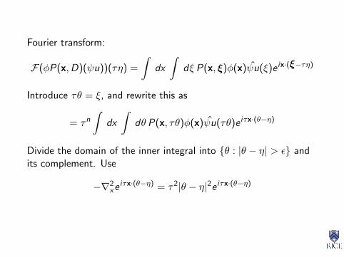
Fourier transform:

F(φP(x,D)(ψu))(τη) =

∫dx

∫dξ P(x, ξ)φ(x)ψu(ξ)e ix·(ξ−τη)

Introduce τθ = ξ, and rewrite this as

= τn

∫dx

∫dθ P(x, τθ)φ(x)ψu(τθ)e iτx·(θ−η)

Divide the domain of the inner integral into θ : |θ − η| > ε andits complement. Use

−∇2xe iτx·(θ−η) = τ2|θ − η|2e iτx·(θ−η)

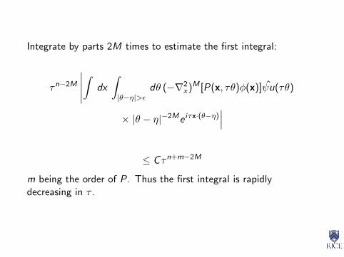
Integrate by parts 2M times to estimate the first integral:

τn−2M

∣∣∣∣∣∫

dx

∫|θ−η|>ε

dθ (−∇2x)M [P(x, τθ)φ(x)]ψu(τθ)

× |θ − η|−2Me iτx·(θ−η)∣∣∣

≤ Cτn+m−2M

m being the order of P. Thus the first integral is rapidlydecreasing in τ .

For the second integral, note that |θ − η| ≤ ε⇒ θ ∈ Ξ, per thedefn of Ξ′. Since X × Ξ is disjoint from the wavefront set of u, fora sequence of constants CN , |ψu(τθ)| ≤ CNτ

−N uniformly for θ inthe (compact) domain of integration, whence the second integral isalso rapidly decreasing in τ . Q. E. D.

And that’s why Kirchhoff migration works, at least in the simplegeometric optics regime.

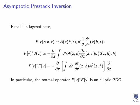
Asymptotic Prestack Inversion

Recall: in layered case,

F [v ]r(h, t) ' A(z(h, t), h)1

2

dr

dz(z(h, t))

F [v ]∗d(z) ' − ∂

∂z

∫dh A(z , h)

∂t

∂z(z , h)d(t(z , h), h)

F [v ]∗F [v ] = − ∂

∂z

[∫dh

dt

dz(z , h)A2(z , h)

]∂

∂z

In particular, the normal operator F [v ]∗F [v ] is an elliptic PDO.

Thus normal operator is asymptotically invertible and you canconstruct approximate least-squares solution to F [v ]r = d :

r ' (F [v ]∗F [v ])−1F [v ]∗d

Relation between r and r : difference is smoother than either. Thusdifference is small if r is oscillatory - consistent with conditionsunder which linearization is accurate.

Analogous construction in simple geometric optics case: due toBeylkin (1985).

Complication: F [v ]∗F [v ] cannot be invertible - becauseWF (F [v ]∗F [v ]r) generally quite a bit “smaller” than WF (r).

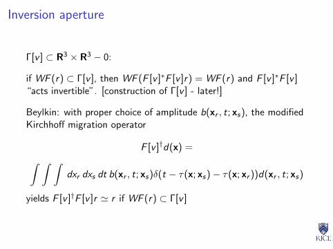
Inversion aperture

Γ[v ] ⊂ R3 × R3 − 0:

if WF (r) ⊂ Γ[v ], then WF (F [v ]∗F [v ]r) = WF (r) and F [v ]∗F [v ]“acts invertible”. [construction of Γ[v ] - later!]

Beylkin: with proper choice of amplitude b(xr , t; xs), the modifiedKirchhoff migration operator

F [v ]†d(x) =∫ ∫ ∫dxr dxs dt b(xr , t; xs)δ(t − τ(x; xs)− τ(x; xr ))d(xr , t; xs)

yields F [v ]†F [v ]r ' r if WF (r) ⊂ Γ[v ]

For details of Beylkin construction: Beylkin, 1985; Miller et al1989; Bleistein, Cohen, and Stockwell 2000; WWS MathFoundations, MGSS notes 1998. All components are by-productsof eikonal solution.

aka: Generalized Radon Transform (“GRT”) inversion, Ray-Borninversion, migration/inversion, true amplitude migration,...

Many extensions, eg. to elasticity: Bleistein, Burridge, deHoop,Lambare,...

Apparent limitation: construction relies on simple geometric optics(no multipathing) - how much of this can be rescued? cf. Part III.

0

500

1000

1500

2000

2500

Dep

th in

Met

ers

0 200 400 600 800 1000 1200 1400CDP

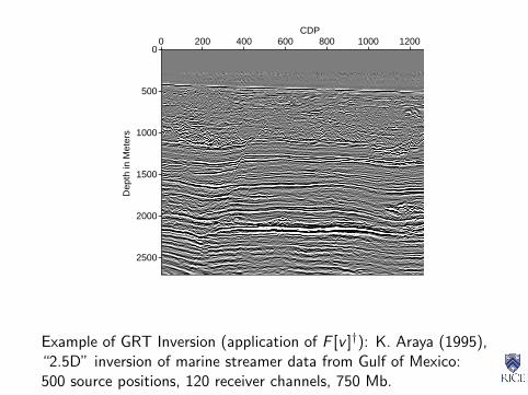
Example of GRT Inversion (application of F [v ]†): K. Araya (1995),“2.5D” inversion of marine streamer data from Gulf of Mexico:500 source positions, 120 receiver channels, 750 Mb.

AgendaSeismic inverse problem: the sedimentary Earth, reflection seismicmeasurements, the acoustic model, linearization, reflectors andreflections idealized via harmonic analysis of singularities

High frequency asymptotics: why adjoints of modeling operatorsare imaging operators (“Kirchhoff migration”). Beylkin-Rakesh-...theory of high frequency asymptotic inversion

Adjoint state imaging with the wave equation: reverse time andreverse depth

Geometric optics, Rakesh’s construction, and asymptotic inversionw/ caustics and multipathing, imaging artifacts, and prestackmigration apres Claerbout.

A step beyond linearization: a mathematical framework for velocityanalysis

Wave Equation Migration

Techniques for computing F [v ]∗:

(i) Reverse time

(ii) Reverse depth

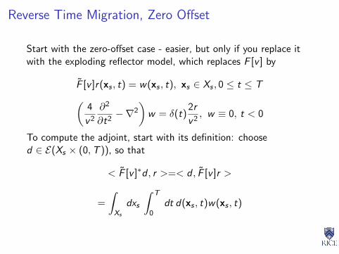
Reverse Time Migration, Zero Offset

Start with the zero-offset case - easier, but only if you replace itwith the exploding reflector model, which replaces F [v ] by

F [v ]r(xs , t) = w(xs , t), xs ∈ Xs , 0 ≤ t ≤ T(4

v 2

∂2

∂t2−∇2

)w = δ(t)

2r

v 2, w ≡ 0, t < 0

To compute the adjoint, start with its definition: choosed ∈ E(Xs × (0,T )), so that

< F [v ]∗d , r >=< d , F [v ]r >

=

∫Xs

dxs

∫ T

0dt d(xs , t)w(xs , t)

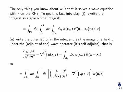
The only thing you know about w is that it solves a wave equationwith r on the RHS. To get this fact into play, (i) rewrite theintegral as a space-time integral:

=

∫R3

dx

∫ T

0dt

∫Xs

dxs d(xs , t)δ(x− xs)w(x, t)

(ii) write the other factor in the integrand as the image of a field qunder the (adjoint of the) wave operator (it’s self-adjoint), that is,(

4

v 2

∂2

∂t2−∇2

)q(x, t) =

∫Xs

dxs d(xs , t)δ(x− xs)

so

=

∫R3

dx

∫ T

0dt

[(4

v 2(x)

∂2

∂t2−∇2

)q(x, t)

]w(x, t)

(iii) integrate by parts

=

∫R3

dx

∫ T

0dt

[(4

v 2(x)

∂2

∂t2−∇2

)w(x, t)

]q(x, t)

which works if q ≡ 0, t > T (final value condition); (iv) use thewave equation for w

=

∫R3

dx

∫ T

0dt

2

v(x)2r(x)δ(t)q(x, t)

(v) observe that you have computed the adjoint:

=

∫R3

dx r(x)

[2

v(x)2q(x, 0)

]=< r , F [v ]∗d >

i.e.

F [v ]∗d =2

v(x)2q(x, 0)

Summary of the computation, with the usual description:

I Use that data as sources, backpropagate in time - i.e. solvethe final value (“reverse time”) problem(

4

v 2

∂2

∂t2−∇2

)q(x, t) =

∫Xs

dxs d(xs , t)δ(x−xs), q ≡ 0, t > T

I read out the “image” (= adjoint output) at t = 0:

F [v ]∗d =2

v(x)2q(x, 0)

Note: The adjoint (time-reversed) field q is not the physical field(δu) run backwards in time, contrary to some imputations in theliterature.

Historical Remarks

I Known as “two way reverse time finite difference poststackmigration” in geophysical literature (Whitmore, 1982)

I uses full (two way) wave equation, propagates adjoint fieldbackwards in time, generally implemented using finitedifference discretization.

I Same as “adjoint state method”, Lions 1968, Chavent 1974for control and inverse problems for PDEs - much earlier forcontrol of ODEs - Lailly, Tarantola ’80s.

I My buddy Tapia says: all you’re doing is transposing a matrix!True (after discretization), but it’s important that thesematrices are triangular, so can be implemented by recursions -forward for simulation, backwards for adjoint.

Reverse Time Migration, Prestack

A slightly messier computation computes the adjoint of F [v ] (i.e.multioffset or prestack migration):

F [v ]∗d(x) = − 2

v(x)

∫dxs

∫ T

0dt

(∂q

∂t∇2u

)(x, t; xs)

where adjoint field q satisfies q ≡ 0, t ≥ T and

(1

v 2

∂2

∂t2−∇2

)q(x, t; xs) =

∫dxr d(xr , t; xs)δ(x− xr )

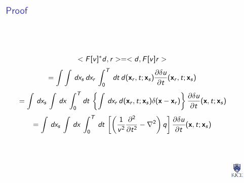
Proof

< F [v ]∗d , r >=< d ,F [v ]r >

=

∫ ∫dxs dxr

∫ T

0dt d(xr , t; xs)

∂δu

∂t(xr , t; xs)

=

∫dxs

∫dx

∫ T

0dt

∫dxr d(xr , t; xs)δ(x− xr )

∂δu

∂t(x, t; xs)

=

∫dxs

∫dx

∫ T

0dt

[(1

v 2

∂2

∂t2−∇2

)q

]∂δu

∂t(x, t; xs)

= −∫

dxs

∫dx

∫ T

0dt

[(1

v 2

∂2

∂t2−∇2

)δu

]∂q

∂t(x, t; xs)

(boundary terms in integration by parts vanish because (i)δu ≡ 0, t << 0; (ii) q ≡ 0, t >> 0; (iii) both vanish for large x, ateach t)

= −∫

dxs

∫dx

∫ T

0dt

(2r

v 2

∂2u

∂t2

∂q

∂t

)(x, t; xs)

= −∫

dxs

∫dx r(x)

2

v 2(x)

∫ T

0dt

(∂2u

∂t2

∂q

∂t

)(x, t; xs)

=< r ,F [v ]∗d >

q.e.d.

Implementation

Algorithm: finite difference or finite element discretization in x,finite difference time stepping.

I For each xs , solve wave equation for u forward in t, recordfinal (t=T) Cauchy data, also (for example) Dirichletboundary data.

I Step u and q backwards in time together; at each time step,data serves as source for q (“backpropagate data”)

I During backwards time stepping, accumulate (approximationsto)

Q(x)+ =2

v 2(x)

∫ T

0dt

(∂2u

∂t2

∂q

∂t

)(x, t; xs)

(“crosscorrelate reference and backpropagated field”).

I next xs - after last xs , F [v ]∗d = Q.

Reverse Depth Migration, Zero Offset

aka: depth extrapolation, downward continuation, or simply “waveequation migration”.

Introduced by Claerbout, early 70’s (“swimming pool equation”).Again, assume exploding reflector model:

F [v ]r(xs , t) = w(xs , t), xs ∈ Xs , 0 ≤ t ≤ T(4

v 2

∂2

∂t2−∇2

)w = δ(t)

2r

v 2, w ≡ 0, t < 0

Basic idea: 2nd order wave equation permits waves to move in alldirections, but waves carrying reflected energy are (mostly) movingup. Should satisfy a 1st order equation for wave motion in onedirection.

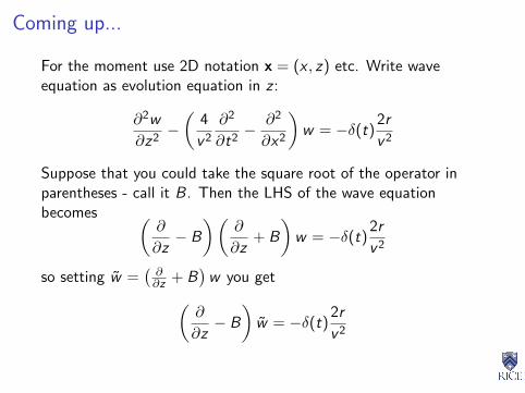
Coming up...

For the moment use 2D notation x = (x , z) etc. Write waveequation as evolution equation in z :

∂2w

∂z2−(

4

v 2

∂2

∂t2− ∂2

∂x2

)w = −δ(t)

2r

v 2

Suppose that you could take the square root of the operator inparentheses - call it B. Then the LHS of the wave equationbecomes (

∂

∂z− B

)(∂

∂z+ B

)w = −δ(t)

2r

v 2

so setting w =(∂∂z + B

)w you get(

∂

∂z− B

)w = −δ(t)

2r

v 2

Some issues

This might be the required equation for upcoming waves.

Two major problems: (i) how the h–l do you take the square rootof a PDO?

(ii) what guarantees that the equation just written governsupcoming waves?

Answers to be found in the theory of ΨDOs!

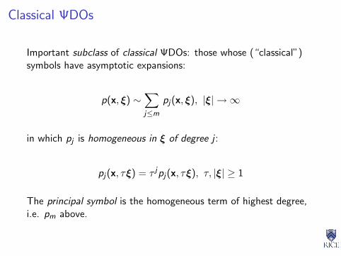
Classical ΨDOs

Important subclass of classical ΨDOs: those whose (“classical”)symbols have asymptotic expansions:

p(x, ξ) ∼∑j≤m

pj(x, ξ), |ξ| → ∞

in which pj is homogeneous in ξ of degree j :

pj(x, τξ) = τ jpj(x, τξ), τ, |ξ| ≥ 1

The principal symbol is the homogeneous term of highest degree,i.e. pm above.

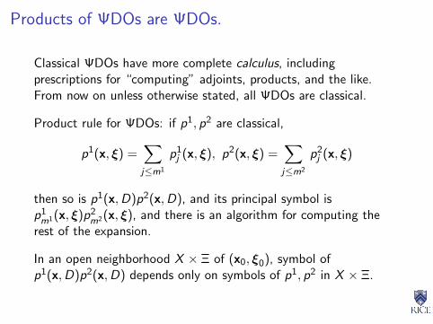
Products of ΨDOs are ΨDOs.

Classical ΨDOs have more complete calculus, includingprescriptions for “computing” adjoints, products, and the like.From now on unless otherwise stated, all ΨDOs are classical.

Product rule for ΨDOs: if p1, p2 are classical,

p1(x, ξ) =∑j≤m1

p1j (x, ξ), p2(x, ξ) =

∑j≤m2

p2j (x, ξ)

then so is p1(x,D)p2(x,D), and its principal symbol isp1m1(x, ξ)p2

m2(x, ξ), and there is an algorithm for computing therest of the expansion.

In an open neighborhood X × Ξ of (x0, ξ0), symbol ofp1(x,D)p2(x,D) depends only on symbols of p1, p2 in X × Ξ.

Consequence: if a(x,D) has an asymptotic expansion and is oforder m ∈ R, and am(x0, ξ0) > 0 in P ⊂ Rn × Rn − 0, then thereexists b(x,D) of order m/2 with asymptotic expansion for which

(a(x,D)− b(x,D)b(x,D))u ∈ E(Rn)

for any u ∈ E ′(Rn) with WF (u) ⊂ P.

Moreover, bm/2(x, ξ) =√

am(x, ξ), (x, ξ) ∈ P. Will call b amicrolocal square root of a.

Similar construction: if a(x, ξ) 6= 0 in P, then there is c(x,D) oforder −m so that

c(x,D)a(x,D)u − u, a(x,D)c(x,D)u − u ∈ E(Rn)

for any u ∈ E ′(Rn) with WF (u) ⊂ P.

Moreover, c−m(x, ξ) = 1/am(x, ξ), (x, ξ) ∈ P. Will call b amicrolocal inverse of a.

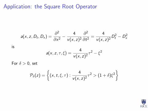
Application: the Square Root Operator

a(x , z ,Dt ,Dx) =∂2

∂x2− 4

v(x , z)2

∂2

∂t2=

4

v(x , z)2D2

t − D2x

is

a(x , z , τ, ξ) =4

v(x , z)2τ2 − ξ2

For δ > 0, set

Pδ(z) =

(x , t, ξ, τ) :

4

v(x , z)2τ2 > (1 + δ)ξ2

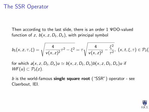
The SSR Operator

Then according to the last slide, there is an order 1 ΨDO-valuedfunction of z , b(x , z ,Dt ,Dx), with principal symbol

b1(x , z , τ, ξ) =

√4

v(x , z)2τ2 − ξ2 = τ

√4

v(x , z)2− ξ2

τ2, (x , t, ξ, τ) ∈ Pδ(z)

for which a(x , z ,Dt ,Dx)u ' b(x , z ,Dt ,Dx)b(x , z ,Dt ,Dx)u ifWF (u) ⊂ Pδ(z).

b is the world-famous single square root (“SSR”) operator - seeClaerbout, IEI.

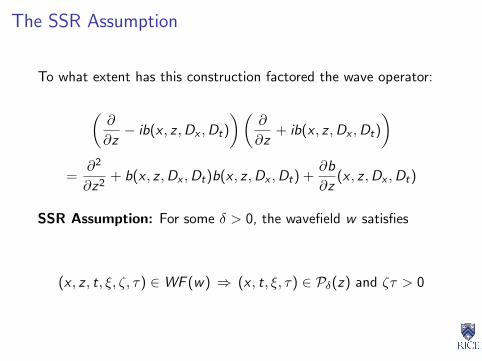
The SSR Assumption

To what extent has this construction factored the wave operator:

(∂

∂z− ib(x , z ,Dx ,Dt)

)(∂

∂z+ ib(x , z ,Dx ,Dt)

)=

∂2

∂z2+ b(x , z ,Dx ,Dt)b(x , z ,Dx ,Dt) +

∂b

∂z(x , z ,Dx ,Dt)

SSR Assumption: For some δ > 0, the wavefield w satisfies

(x , z , t, ξ, ζ, τ) ∈WF (w) ⇒ (x , t, ξ, τ) ∈ Pδ(z) and ζτ > 0

This statement has a ray-theoretic interpretation (which willeventually make sense): rays carrying significant energy arenowhere horizontal. Along any such ray, z decreases as t increases- coming up!

w(x , z , t) =

(∂

∂z+ ib(x , z ,Dx ,Dt)

)w(x , z , t)

b(x , z ,Dx ,Dt)b(x , z ,Dx ,Dt)w '(

4

v(x , z)2D2

t − D2x

)w

with a smooth error, so(∂

∂z− ib(x , z ,Dx ,Dt)

)w(x , z , t) = −2r(x , z)

v(x , z)2δ(t)

+i

(∂

∂zb(x , z ,Dx ,Dt)

)w(x , z , t)

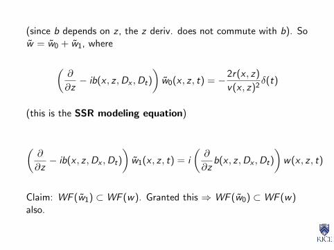
(since b depends on z , the z deriv. does not commute with b). Sow = w0 + w1, where

(∂

∂z− ib(x , z ,Dx ,Dt)

)w0(x , z , t) = −2r(x , z)

v(x , z)2δ(t)

(this is the SSR modeling equation)

(∂

∂z− ib(x , z ,Dx ,Dt)

)w1(x , z , t) = i

(∂

∂zb(x , z ,Dx ,Dt)

)w(x , z , t)

Claim: WF (w1) ⊂WF (w). Granted this ⇒ WF (w0) ⊂WF (w)also.

Upshot: SSR modeling

F0[v ]r(xs , zs , t) = w0(xs , zs , t)

produces the same singularities (i.e. the same waves) as explodingreflector modeling, so is as good a basis for migration.

SSR migration: assume that sources all lie on zs = 0.

< F0[v ]∗d , r >=< d , F0[v ]r >

=

∫dxs

∫dt d(xs , t)w0(xs , 0, t)

=

∫dxs

∫dt

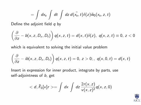
∫dz ¯d(xs , t)δ(z)w0(xs , z , t)

Define the adjoint field q by(∂

∂z− b(x , z ,Dx ,Dt)

)q(x , z , t) = d(x , t)δ(z), q(x , z , t) ≡ 0, z < 0

which is equivalent to solving the initial value problem(∂

∂z− ib(x , z ,Dx ,Dt)

)q(x , z , t) = 0, z > 0; , q(x , 0, t) = d(x , t)

Insert in expression for inner product, integrate by parts, useself-adjointness of b, get

< d , F0[v ]r >=

∫dx

∫dz

2r(x , z)

v(x , z)2q(x , z , 0)

whence

F0[v ]∗d(x , z) =2

v(x , z)2q(x , z , 0)

Standard description of the SSR migration algorithm:

I downward continue data (i.e. solve for q)

I image at t = 0.

The art of SSR migration: computable approximations tob(x , z ,Dx ,Dt) - swimming pool operator, many successors.

Proof of the Claim

Unfinished business: proof of claim

Depends on celebrated Propagation of Singularities theorem ofHormander (1970).

Given symbol p(x, ξ), order m, with asymptotic expansion, definebicharateristics as solutions (x(t), ξ(t)) of Hamiltonian system

dx

dt=∂p

∂ξ(x, ξ),

dξ

dt= −∂p

∂x(x, ξ)

with p(x(t), ξ(t)) ≡ 0.

Theorem: Suppose p(x,D)u = f , and suppose that fort0 ≤ t ≤ t1, (x(t), ξ(t)) /∈WF (f ). Then either(x(t), ξ(t)) : t0 ≤ t ≤ t1 ⊂WF (u) or(x(t), ξ(t)) : t0 ≤ t ≤ t1 ⊂ T ∗(Rn)−WF (u).

P of S has at least two distinct proofs:

I Nirenberg, 1972

I Hormander, 1970 (in Taylor, 1981)

Proof of claim: check that bicharacteristics for SSR operator arejust upcoming rays of geom. optics for wave equation. These passinto t < 0 where RHS is smooth, also initial condn at large z issmooth - so each ray has one “end” outside of WF (w1). If raycarries singularity, must pass of WF of w , but then it’s entirelycontained by P of S applied to w . q. e. d.

Reverse Depth Migration, Prestack

Nonzero offset (“prestack”): starting point is integralrepresentation of the scattered field

F [v ]r(xr , t; xs) =∂2

∂t2

∫dx

2r(x)

v(x)2

∫ds G (xr , t − s; x)G (xs , s; x)

By analogy with zero offset case, would like to view this as“exploding reflectors in both directions”: reflectors propagateenergy upward to sources and to receivers.

However can’t do this because reflection location is same for both.

The “survey sinking” idea

Bold stroke: introduce a new space variable y (a “sunken source”,think of x as a “sunken receiver”), define

F [v ]R(xr , t; xs) =∂2

∂t2

∫ ∫dx dy R(x, y)

∫ds G (xr , t−s; x)G (xs , s; y)

and note that F [v ]R = F [v ]r if

R(x, y) =2r

v 2

(x + y

2

)δ(x− y)

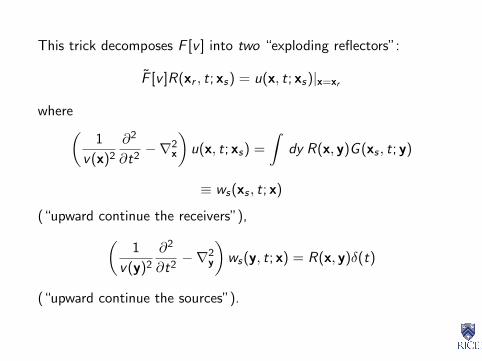
This trick decomposes F [v ] into two “exploding reflectors”:

F [v ]R(xr , t; xs) = u(x, t; xs)|x=xr

where(1

v(x)2

∂2

∂t2−∇2

x

)u(x, t; xs) =

∫dy R(x, y)G (xs , t; y)

≡ ws(xs , t; x)

(“upward continue the receivers”),(1

v(y)2

∂2

∂t2−∇2

y

)ws(y, t; x) = R(x, y)δ(t)

(“upward continue the sources”).

This factorization of F [v ] (r 7→ R 7→ F [v ]R) leads to a reversetime computation of adjoint F [v ]∗ - will discuss this later.

It’s equally possible to continue the receivers first, then thesources, which leads to(

1

v(y)2

∂2

∂t2−∇2

y

)u(xr , t; y) =

∫dx R(x, y)G (xr , t; x)

≡ wr (xr , t; y)

(“upward continue the sources”),(1

v(x)2

∂2

∂t2−∇2

x

)wr (x, t; y) = R(x, y)δ(t)

(“upward continue the receivers”).

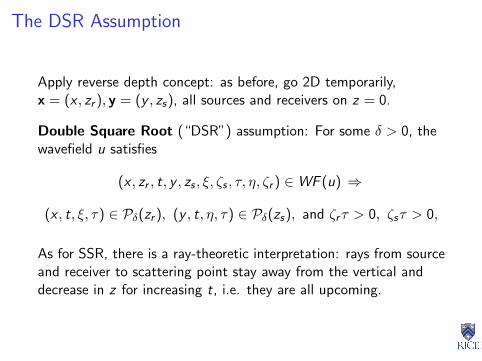
The DSR Assumption

Apply reverse depth concept: as before, go 2D temporarily,x = (x , zr ), y = (y , zs), all sources and receivers on z = 0.

Double Square Root (“DSR”) assumption: For some δ > 0, thewavefield u satisfies

(x , zr , t, y , zs , ξ, ζs , τ, η, ζr ) ∈WF (u) ⇒

(x , t, ξ, τ) ∈ Pδ(zr ), (y , t, η, τ) ∈ Pδ(zs), and ζrτ > 0, ζsτ > 0,

As for SSR, there is a ray-theoretic interpretation: rays from sourceand receiver to scattering point stay away from the vertical anddecrease in z for increasing t, i.e. they are all upcoming.

Since z will be singled out (and eventually R(x, y) will have afactor of δ(x, y)), impose the constraint that

R(x , z , x , zs) = R(x , y , z)δ(z − zs)

Define upcoming projections as for SSR:

ws =

(∂

∂zs+ ib(y , zs ,Dy ,Dt)

)ws ,

wr =

(∂

∂zr+ ib(x , zr ,Dx ,Dt)

)wr ,

u =

(∂

∂zs+ ib(y , zs ,Dy ,Dt)

)(∂

∂zr+ ib(x , zr ,Dx ,Dt)

)u

Except for lower order commutators which we justify throwingaway as before,(

∂

∂zs− ib(y , zs ,Dy ,Dt)

)ws = Rδ(zr − zs)δ(t),

(∂

∂zr− ib(x , zr ,Dx ,Dt)

)wr = Rδ(zr − zs)δ(t),(

∂

∂zr− ib(x , zr ,Dx ,Dt)

)u = ws(

∂

∂zs− ib(y , zs ,Dy ,Dt)

)u = wr

Initial (final) conditions are that wr , ws , and u all vanish for large z- the equations are to be solve in decreasing z (“upwardcontinuation”).

Simultaneous upward continuation:

∂

∂zu(x , z , t; y , z) =

∂

∂zru(x , zr , t; y , z)|z=zr +

∂

∂zru(x , z , t; y , zs)|z=zs

= [ib(x , zr ,Dx ,Dt)u + ws + ib(y , zs ,Dy ,Dt)u + wr ]zr =zs=z

Since ws(y , z , t; x , z) = wr (x , z , t; y , z) = R(x , y , z)δ(t), u is seento satisfy the

DSR modeling equation:(∂

∂z− ib(x , z ,Dx ,Dt)− ib(y , z ,Dy ,Dt)

)u(x , z , t; y , z) = 2R(x , y , z)δ(t)

F [v ]R(xr , t; xs) = u(xr , 0, t; xs , 0)

DSR Migration

Computation of adjoint follows same pattern as for SSR, and leadsto

DSR migration equation: solve(∂

∂z− ib(x , z ,Dx ,Dt)− ib(y , z ,Dy ,Dt)

)q(x , y , z , t) = 0

in increasing z with initial condition at z = 0:

q(xr , xs , 0, t) = d(xr , xs , t)

Then F [v ]∗d(x , y , z) = q(x , y , z , 0)

The physical DSR model has R(x , y , z) = r(x , z)δ(x − y), so finalstep in DSR computation of F [v ]∗ is adjoint of r 7→ R:

F [v ]∗d(x , z) = q(x , x , z , 0)

Standard description of DSR migration

(See Claerbout, IEI):

I downward continue sources and receivers (solve DSRmigration equation)

I image at t = 0 and zero offset (x = y)

Another moniker: “survey sinking”: DSR field q is (related to) thefield that you would get by conducting the survey with sources andreceivers at depth z . At any given depth, the zero-offset, time-zeropart of the field is the instantaneous response to scatterers onwhich source = receiver is sitting, therefore constitutes an image.

As for SSR, the art of DSR migration is in the approximation ofthe DSR operator.

Remarks

Stolk and deHoop (2001) derived DSR modeling and migration viaa more systematic argument than that used here, involving ΨDOmatrix factorization of the wave equation written as a first orderevolution system in z . This idea goes back to Taylor (1975) whoused it to show that singularities propagating alongbicharacteristics reflect as expected at boundaries.

Stolk (2003) has also carried out a very careful global constructionof a family of SSR ΨDOs which are of non-classical type atnear-horizontal directions (“nearly evanescent waves”). Thisconstruction should lead to more reliable discretizations.

The last part of the course will present the various apparentlyad-hoc “prestack modeling” ideas within a unified framework.

AgendaSeismic inverse problem: the sedimentary Earth, reflection seismicmeasurements, the acoustic model, linearization, reflectors andreflections idealized via harmonic analysis of singularities

High frequency asymptotics: why adjoints of modeling operatorsare imaging operators (“Kirchhoff migration”). Beylkin-Rakesh-...theory of high frequency asymptotic inversion

Adjoint state imaging with the wave equation: reverse time andreverse depth

Geometric optics, Rakesh’s construction, and asymptotic inversionw/ caustics and multipathing, imaging artifacts, and prestackmigration apres Claerbout.

A step beyond linearization: a mathematical framework for velocityanalysis

Why Beylkin isn’t enough

The theory developed by Beylkin and others cannot be the end ofthe story:

I The “single ray” hypotheses generally fails in the presence ofstrong refraction.

I B. White, “The Stochastic Caustic” (1982): For “random butsmooth” v(x) with variance σ, points at distance O(σ−2/3)from source have more than one ray connecting to source,with probability 1 - multipathing associated with formation ofcaustics = ray envelopes.

I Formation of caustics invalidates asymptotic analysis on whichBeylkin result is based.

Why it matters

I Strong refraction leading to multipathing and causticformation typical of salt (4-5 km/s) intrusion into sedimentaryrock (2-3 km/s) (eg. Gulf of Mexico), also chalk tectonics inNorth Sea and elsewhere - some of the most promisingpetroleum provinces!

Escape from simplicity - the Canonical Relation

How do we get away from “simple geometric optics”, SSR, DSR,...- all violated in sufficiently complex (and realistic) models? RakeshComm. PDE 1988, Nolan Comm. PDE 1997: global description ofFδ[v ] as mapping reflectors 7→ reflections.

Y = xs , t, xr (time × set of source-receiver pairs) submfd of R7

of dim. ≤ 5, Π : T ∗(R7)→ T ∗Y the natural projection

supp r ⊂ X ⊂ R3

Canonical relation CFδ[v ] ⊂ T ∗(X ) \ 0 × T ∗(Y ) \ 0 describessingularity mapping properties of F :

(x, ξ, y, η) ∈ CFδ[v ] ⇔

for some u ∈ E ′(X ), (x, ξ) ∈WF (u), and (y, η) ∈WF (Fu)

Geometry of Reflection

Rays of geometric optics: solutions of Hamiltonian system

dX

dt= ∇ΞH(X,Ξ),

dΞ

dt= −∇XH(X,Ξ)

with H(X,Ξ) = 1− v 2(X)|Ξ|2 = 0 (null bicharacteristics).

Characterization of CF :

((x, ξ), (xs , t, xr , ξs, τ, ξr)) ∈ CFδ[v ] ⊂ T ∗(X )− 0 × T ∗(Y )− 0

⇔ there are rays of geometric optics (Xs ,Ξs), (Xr ,Ξr ) and timests , tr so that

Π(Xs(0), t,Xr (t),Ξs(0), τ,Ξr (t)) = (xs , t, xr , ξs , τ, ξr ),

Xs(ts) = Xr (t − tr ) = x, ts + tr = t, Ξs(ts)− Ξr (t − tr )||ξ

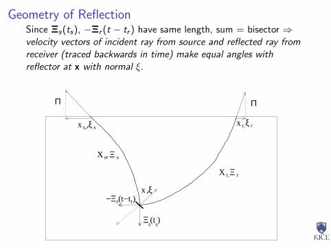
Geometry of ReflectionSince Ξs(ts), −Ξr (t − tr ) have same length, sum = bisector ⇒velocity vectors of incident ray from source and reflected ray fromreceiver (traced backwards in time) make equal angles withreflector at x with normal ξ.

(t−t )

X

sΞ (t )

s

X s

x

x x ξ rs, r,sξ,

Ξ s

ξ,

rΞr,

,

ΠΠ

−Ξr r

Geometry of Reflection

Upshot: canonical relation of Fδ[v ] simply enforces theequal-angles law of reflection.

Further, rays carry high-frequency energy, in exactly the fashionthat seismologists imagine.

Finally, Rakesh’s characterization of CF is global: no assumptionsabout ray geometry, other than no forward scattering and nograzing incidence on the acquisition surface Y , are needed.

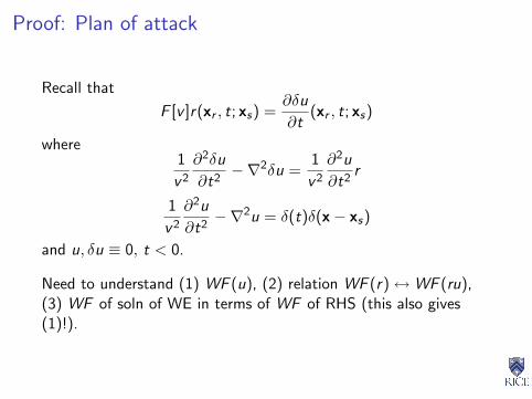
Proof: Plan of attack

Recall that

F [v ]r(xr , t; xs) =∂δu

∂t(xr , t; xs)

where1

v 2

∂2δu

∂t2−∇2δu =

1

v 2

∂2u

∂t2r

1

v 2

∂2u

∂t2−∇2u = δ(t)δ(x− xs)

and u, δu ≡ 0, t < 0.

Need to understand (1) WF (u), (2) relation WF (r)↔WF (ru),(3) WF of soln of WE in terms of WF of RHS (this also gives(1)!).

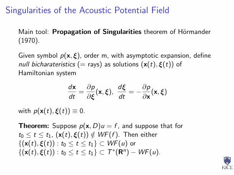
Singularities of the Acoustic Potential Field

Main tool: Propagation of Singularities theorem of Hormander(1970).

Given symbol p(x, ξ), order m, with asymptotic expansion, definenull bicharateristics (= rays) as solutions (x(t), ξ(t)) ofHamiltonian system

dx

dt=∂p

∂ξ(x, ξ),

dξ

dt= −∂p

∂x(x, ξ)

with p(x(t), ξ(t)) ≡ 0.

Theorem: Suppose p(x,D)u = f , and suppose that fort0 ≤ t ≤ t1, (x(t), ξ(t)) /∈WF (f ). Then either(x(t), ξ(t)) : t0 ≤ t ≤ t1 ⊂WF (u) or(x(t), ξ(t)) : t0 ≤ t ≤ t1 ⊂ T ∗(Rn)−WF (u).

Source to Field

RHS of wave equation for u = δ function in x, t. WF set =(x, t, ξ, τ) : x = xs , t = 0 - i.e. no restriction on covector part.

⇒ (x, t, ξ, τ) ∈WF (u) iff a ray starting at (xs , 0) passes over(x, t) - i.e. (x, t) lies on the “light cone” with vertex at (xs , 0).Symbol for wave op is p(x, t, ξ, τ) = 1

2 (τ2 − v 2(x)|ξ|2), soHamilton’s equations for null bicharacteristics are

dX

dt= −v 2(X)Ξ,

dΞ

dt= ∇ log v(X)

Thus ξ is proportional to velocity vector of ray.

[(ξ, τ) normal to light cone.]

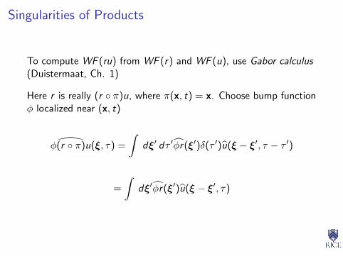
Singularities of Products

To compute WF (ru) from WF (r) and WF (u), use Gabor calculus(Duistermaat, Ch. 1)

Here r is really (r π)u, where π(x, t) = x. Choose bump functionφ localized near (x, t)

φ(r π)u(ξ, τ) =

∫dξ′ dτ ′φr(ξ′)δ(τ ′)u(ξ − ξ′, τ − τ ′)

=

∫dξ′φr(ξ′)u(ξ − ξ′, τ)

This will decay rapidly as |(ξ, τ)| → ∞ unless (i) you can find(x′, ξ′) ∈WF (r) so that x, x′ ∈ π(suppφ), ξ − ξ′ ∈WF (u), i.e.(ξ, τ) ∈WF (r π) + WF (u), or (ii) ξ ∈WF (r) or (ξ, τ) ∈WF (u).

Possibility (ii) will not contribute, so effectively

WF ((r π)u) = (x, ts , ξ + Ξs(ts), ·) : (x, ξ) ∈WF (r), x = Xs(ts)

for a ray (Xs ,Ξs) with Xs(0) = xs , some τ .

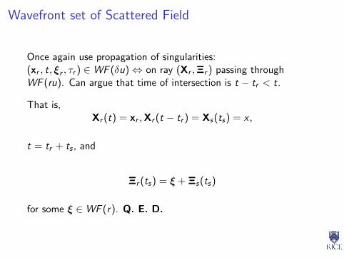
Wavefront set of Scattered Field

Once again use propagation of singularities:(xr , t, ξr , τr ) ∈WF (δu)⇔ on ray (Xr ,Ξr ) passing throughWF (ru). Can argue that time of intersection is t − tr < t.

That is,Xr (t) = xr ,Xr (t − tr ) = Xs(ts) = x ,

t = tr + ts , and

Ξr (ts) = ξ + Ξs(ts)

for some ξ ∈WF (r). Q. E. D.

Rakesh’s Thesis

Rakesh also showed that F [v ] is a Fourier Integral Operator =class of oscillatory integral operators, introduced by Hormanderand others in the ’70s to describe the solutions of nonelliptic PDEs.

Phases and amplitudes of FIOs satisfy certain restrictive conditions.Canonical relations have geometric description similar to that ofF [v ]. Adjoint of FIO is FIO with inverse canonical relation.

ΨDOs are special FIOs.

Composition of FIOs does not yield an FIO in general. Beylkin hadshown that F [v ]∗F [v ] is FIO (ΨDO, actually) under simple raygeometry hypothesis - but this is only sufficient. Rakesh noted thatthis follows from general results of Hormander: simple raygeometry ⇔ canonical relation is graph of ext. deriv. of phasefunction.

The Shell Guys and TIC

Smit, tenKroode and Verdel (1998): provided that

I source, receiver positions (xs , xr ) form an open 4D manifold(“complete coverage” - all source, receiver positions at leastlocally), and

I the Traveltime Injectivity Condition (“TIC”) holds:C−1

F [v ] ⊂ T ∗Y \ 0 × T ∗X \ 0 is a function - that is, initialdata for source and receiver rays and total travel timetogether determine reflector uniquely.

then F [v ]∗F [v ] is ΨDO ⇒ application of F [v ]∗ produces image,and F [v ]∗F [v ] has microlocal parametrix (“asymptotic inversion”).

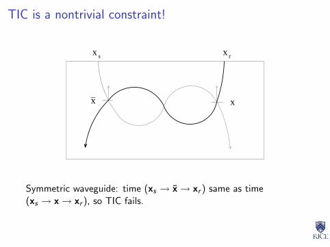
TIC is a nontrivial constraint!

x x

x xs r

Symmetric waveguide: time (xs → x→ xr ) same as time(xs → x→ xr ), so TIC fails.

Stolk’s Thesis

Stolk (2000): for dim=2, under “complete coverage” hypothesis, vfor which F [v ]∗F [v ] = [ΨDO + rel. smoothing op] open, dense setin C∞(R2) (without assuming TIC!). Conjecture: same for dim=3.

Also, for any dim, v for which F [v ]∗F [v ] is FIO open, dense inC∞(R2).

Operto’s Thesis

Application of F [v ]∗ involves accounting for all rays connectingsource and receiver with reflectors.

Standard practice still attempts imaging with single choice of raypair (shortest time, max energy,...).

Operto et al (2000) give nice illustration that all rays must beincluded in general to obtain good image.

Nolan’s Thesis

Limitation of Smit-tenKroode-Verdel: most idealized dataacquisition geometries violate “complete coverage”: for example,idealized marine streamer geometry (src-recvr submfd is 3D)

Nolan (1997): result remains true without “complete coverage”condition: requires only TIC plus addl condition so that projectionCF [v ] → T ∗Y is embedding - but examples violating TIC are mucheasier to construct when source-receiver submfd has positivecodim.

Sinister Implication: When data is just a single gather - commonshot, common offset - image may contain artifacts, i.e. spuriousreflectors not present in model.

Horrible Example

Synthetic 2D Example (see Stolk and WWS, Geophysics 2004 forthis and other horrible expls)

Strongly refracting acoustic lens (v) over horizontal reflector (r),Sobs = F [v ]r .

(i) for open source-receiver set, F [v ]∗Sobs = good image ofreflector - within limits of finite frequency implied by numericalmethod, F [v ]∗F [v ] acts like ΨDO;

(ii) for common offset submfd (codim 1), TIC is violated andWF (F [v ]∗Sobs) is larger than WF (r).

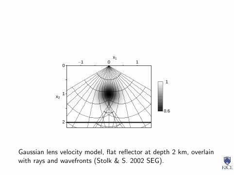
2

1

0

x2

-1 0 1x1

1

0.6

Gaussian lens velocity model, flat reflector at depth 2 km, overlainwith rays and wavefronts (Stolk & S. 2002 SEG).

5

4

timeHsL

-2 -1 0 1 2receiver position HkmL

Typical shot gather - lots of arrivals

1.6

2.0

2.4

x2

0.0 0.4 0.8x1

Image from common offset gather at h = 0.3 - all three ray pairsbelong to the same offset, midpoint, time, midpoint slowness - TICfails, image has “artifact” WF

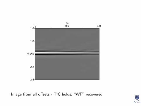
1.6

1.8

2.0

2.2

2.4

x20 0.5 1.0

x1

Image from all offsets - TIC holds, “WF” recovered

What it all means

Note that a gather scheme makes the scattering operatorblock-diagonal: for example with data sorted into common offsetgathers h = (xr − xs)/2,

F [v ] = [Fh1 [v ], ...,FhN[v ]]T , d = [dh1 , ..., dhN

]T

Thus F [v ]∗d =∑

i Fhi[v ]∗dhi

. Otherwise put: to form image,migrate ith gather (apply migration operator Fhi

[v ]∗, then stackindividual migrated images.

Horrible Examples show that individual offset gather images maycontain nonphysical apparent reflectors (artifacts).

Smit-tenKroode-Verdel, Nolan, Stolk: if TIC holds, then theseartifacts are not stationary with respect to the gather parameter,hence stack out (interfere destructively) in final image.

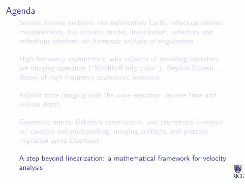
AgendaSeismic inverse problem: the sedimentary Earth, reflection seismicmeasurements, the acoustic model, linearization, reflectors andreflections idealized via harmonic analysis of singularities

High frequency asymptotics: why adjoints of modeling operatorsare imaging operators (“Kirchhoff migration”). Beylkin-Rakesh-...theory of high frequency asymptotic inversion

Adjoint state imaging with the wave equation: reverse time andreverse depth

Geometric optics, Rakesh’s construction, and asymptotic inversionw/ caustics and multipathing, imaging artifacts, and prestackmigration apres Claerbout.

A step beyond linearization: a mathematical framework for velocityanalysis

Velocity AnalysisPartially linearized seismic inverse problem (“velocity analysis”):given observed seismic data d , find smooth velocityv ∈ E(X ),X ⊂ R3 oscillatory reflectivity r ∈ E ′(X ) so that

F [v ]r ' d

Acoustic partially linearized model: acoustic potential field u andits perturbation δu solve(

1

v 2

∂2

∂t2−∇2

)u = δ(t)δ(x− xs),

(1

v 2

∂2

∂t2−∇2

)δu = 2r∇2u

plus suitable bdry and initial conditions.

F [v ]r =∂δu

∂t

∣∣∣∣Y

data acquisition manifold Y = (xr , t; xs) ⊂ R7, dimn Y ≤ 5(many idealizations here!).

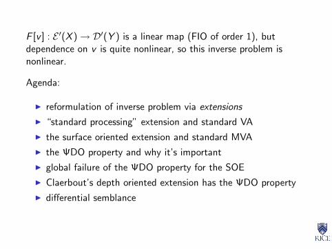
F [v ] : E ′(X )→ D′(Y ) is a linear map (FIO of order 1), butdependence on v is quite nonlinear, so this inverse problem isnonlinear.

Agenda:

I reformulation of inverse problem via extensions

I “standard processing” extension and standard VA

I the surface oriented extension and standard MVA

I the ΨDO property and why it’s important

I global failure of the ΨDO property for the SOE

I Claerbout’s depth oriented extension has the ΨDO property

I differential semblance

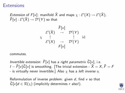
Extensions

Extension of F [v ]: manifold X and maps χ : E ′(X )→ E ′(X ),F [v ] : E ′(X )→ D′(Y ) so that

F [v ]E ′(X ) → D′(Y )

χ ↑ ↑ idE ′(X ) → D′(Y )

F [v ]

commutes.

Invertible extension: F [v ] has a right parametrix G [v ], i.e.I − F [v ]G [v ] is smoothing. [The trivial extension - X = X , F = F- is virtually never invertible.] Also χ has a left inverse η.

Reformulation of inverse problem: given d , find v so thatG [v ]d ∈ R(χ) (implicitly determines r also!).

Example 1: Standard VA extension

Treat each CMP as if it were the result of an experiment performedover a layered medium, but permit the layers to vary with midpoint.

Thus v = v(z), r = r(z) for purposes of analysis, but at the endv = v(xm, z), r = r(xm, z).

F [v ]R(xm, h, t) ' A(xm, h, z(xm, h, t))R(xm, z(xm, h, t))

Here z(xm, h, t) is the inverse of the 2-way traveltime

t(xm, h, z) = 2τ(xm + (h, 0, z), xm)v=v(xm,z)

computed with the layered velocity v(xm, z), i.e.z(xm, h, t(xm, h, z

′)) = z ′.

That is, F [v ] is a change of variable followed by multiplication by asmooth function. NB: industry standard practice is to use verticaltraveltime t0 instead of z for depth variable.

Can write this as F [v ] = F S∗, where F [v ] = N[v ]−1M[v ] has rightparametrix G [v ] = M[v ]N[v ]:

N[v ] = NMO operator N[v ]d(xm, h, z) = d(xm, h, t(xm, h, z))

M[v ] = multiplication by A

S = stacking operator

Sf (xm, z) =

∫dh f (xm, h, z), S∗r(xm, h, z) = r(x, z)

Identify as extension: F [v ], G [v ] as above,X = xm, z,H = h, X = X × H, χ = S∗, η = S - the invertibleextension properties are clear.

Standard names for the Standard VA extension objects: F [v ] =“inverse NMO”, G [v ] = “NMO” [often the multiplication op M[v ]is neglected]; η = “stack”, χ = “spread”

How this is used for velocity analysis: Look for v that makesG [v ]d ∈ R(χ)

So what is R(χ)? χ[r ](xm, z , h) = r(xm, z) Anything in range of χis independent of h. Practical issues ⇒ replace “independent of”with “smooth in”.

Flatten them gathers!

Inverse problem reduced to: adjust v to make G [v ]dobs smooth inh, i.e. flat in z , h display for each xm (NMO-corrected CMP).

Replace z with t0, v with vRMS em localizes computation:reflection through xm, t0, 0 flattened by adjusting vRMS(xm, t0) ⇒1D search, do by visual inspection.

Various aids - NMO corrected CMP gathers, velocity spectra, etc.

See: Claerbout: Imaging the Earth’s Interior

WWS: MGSS 2000 notes

0.6

0.8

1.0

1.2

1.4

1.6

1.8

time

(s)

10 20 30 40 50channel

,

0

0.5

1.0

1.5

2.0

time

(s)

0.5 1.0 1.5 2.0 2.5offset (km)

Left: part of survey (d) from North Sea (thanks: Shell Research),lightly preprocessed.Right: restriction of G [v ]d to xm = const (function of depth,offset): shows rel. sm’ness in h (offset) for properly chosen v .

Example 2: Surface oriented or standard MVA extension

. This only works where Earth is “nearly layered”. Where this fails,replace NMO by prestack migration.

Shot version: Σs = set of shot locations, X = X × Σs ,χ[r ](x, xs) = r(x).

F [v ]r(xr , t, xs) =∂2

∂t2

∫dx r(x, xs)

∫ds G (xr , t − s; x)G (xs , s; x)

Offset version (preferred because it minimizes truncation artifacts):Σh = set of half-offsets in data, X = X × Σh, χ[r ](x,h) = r(x).

F [v ]r(xs , t,h) =∂2

∂t2

∫dx r(x,h)

∫ds G (xs+h, t−s; x)G (xs , s; x)

[Parametrize data with source location xs , time t, offset h.] NB:note that both versions are “block diagonal” - family of operators(FIOs) parametrized by xs or h.

Properties of SOE

Beylkin (1985), Rakesh (1988): if ‖v‖C2(X ) “not too big”, then

I F has the ΨDO property: F F ∗ is ΨDO

I singularities of F F ∗d ⊂ singularities of d

I straightforward construction of right parametrix G = F ∗Q, Q= ΨDO, also as generalized Radon Transform - explicitlycomputable.

Range of χ (offset version): r(x,h) independent of h ⇒“semblance principle”: find v so that G [v ]dobs is independent of h.Practical limitations ⇒ replace “independent of h” by “smooth inh”.

Industrial MVA

Application of these ideas = industrial practice of migrationvelocity analysis.

Idea: twiddle v until G [v ]dobs is smooth in h.

Since it is hard to inspect G [v ]dobs(x , y , z , h), pull out subset forconstant x , y = common image gather (“CIG”): display functionof z , h for fixed x , y . These play same role as NMO corrected CMPgathers in layered case.

Try to adjust v so that selected CIGs are flat - just as in StandardVA. This is much harder, as there is no RMS velocity trick tolocalize the computation - each CIG depends globally on v .

Description, some examples: Yilmaz, Seismic Data Processing.

Bad newsNolan (1997): big trouble! In general, standard extension does nothave the ΨDO property. Geometric optics analysis: for ‖v‖C2(X )

“large”, multiple rays connect source, receiver to reflecting pointsin X ; block diagonal structure of F [v ]⇒ info necessary todistinguish multiple rays is projected out.

2

1

0

x2

-1 0 1x1

1

0.6

Example (Stolk & WWS, 2001): Gaussian lens over flat reflectorat depth z (r(x) = δ(x1 − z), x1 = depth).

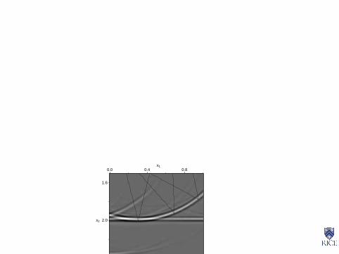
1.6

2.0

2.4

x2

0.0 0.4 0.8x1

,

1.6

2.0

2.4

x2

0 1 2offset

3,2

3,1

1,2

2,1

3,3

1,1

travel time # s,r

Left: Const. h slice of G d : several refl. points corresponding tosame singularity in dobs.Right: CIG (const. x , y slice) of G d : not smooth in h!

Example 3: Claerbout’s depth oriented extension

Standard MVA extension only works when Earth has simple raygeometry. Claerbout proposed alternative extension:

Σd = somewhat arbitrary set of vectors near 0 (“offsets”),X = X × Σd , χ[r ](x,h) = r(x)δ(h), η[r ](x) = r(x, 0)

F [v ]r(xs , t, xr ) =∂2

∂t2

∫dx

∫Σd

dh r(x,h)

∫ds G (xs , t−s; x+2h)G (xr , s; x)

=∂2

∂t2

∫dx

∫x+2Σd

dy r(x, y − x)

∫ds G (xs , t − s; y)G (xr , s; x)

NB: in this formulation, there appears to be too many modelparameters.

Shot record modeling

for each xs solve

F [v ]r(xr , t; xs) = u(x, t; xs)|x=xr

where(1

v(x)2

∂2

∂t2−∇2

x

)u(x, t; xs) =

∫x+2Σd

dy r(x, y)G (y, t; xs)

(1

v(y)2

∂2

∂t2−∇2

y

)G (y, t; xs) = δ(t)δ(xs − y)

Finite difference scheme: form RHS for eqn 1, step u, G forward int.

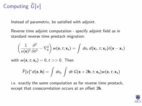
Computing G [v ]

Instead of parametrix, be satisfied with adjoint.

Reverse time adjoint computation - specify adjoint field as instandard reverse time prestack migration:(

1

v(x)2

∂2

∂t2−∇2

x

)w(x, t; xs) =

∫dxr d(xr , t; xs)δ(x− xr )

with w(x, t; xs) = 0, t >> 0. Then

F [v ]∗d(x,h) =

∫dxs

∫dt G (x + 2h, t; xs)w(x, t; xs)

i.e. exactly the same computation as for reverse time prestack,except that crosscorrelation occurs at an offset 2h.

Nomenclature

NB: the “usual computation” of G [v ] is either DSR or a variant ofshot record computation of previous slide using depthextrapolation. h is usually restricted to be horizontal, i.e. h3 = 0.

Common names: shot-geophone or survey-sinking migration (withDSR), or shot record migration.

“Downward continue sources and receivers, image at t = 0, h = 0”

These are what is typically meant by “wave equation migration”!

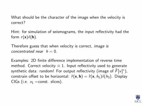
What should be the character of the image when the velocity iscorrect?

Hint: for simulation of seismograms, the input reflectivity had theform r(x)δ(h).

Therefore guess that when velocity is correct, image isconcentrated near h = 0.

Examples: 2D finite difference implementation of reverse timemethod. Correct velocity ≡ 1. Input reflectivity used to generatesynthetic data: random! For output reflectivity (image of F [v ]∗),constrain offset to be horizontal: r(x,h) = r(x, h1)δ(h3). DisplayCIGs (i.e. x1 =const. slices).

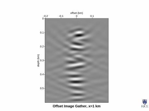
0

0.1

0.2

0.3

0.4

0.5

dept

h (k

m)

-0.2 -0.1 0 0.1offset (km)

Offset Image Gather, x=1 km

,

0

0.1

0.2

0.3

0.4

0.5

dept

h (k

m)

-0.2 -0.1 0 0.1offset (km)

OIG, x=1 km: vel 10% high

,

0

0.1

0.2

0.3

0.4

0.5

dept

h (k

m)

-0.2 -0.1 0 0.1offset (km)

OIG, x=1 km: vel 10% low

Two way reverse time horizontal offset S-G image gathers of datafrom random reflectivity, constant velocity. From left to right:correct velocity, 10% high, 10% low.

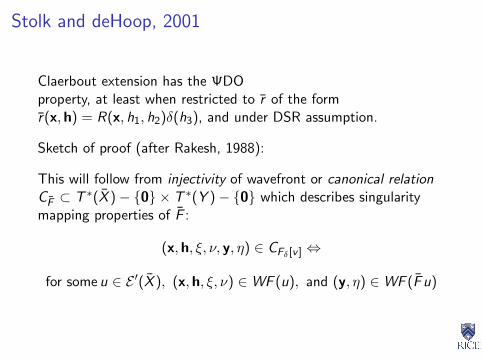
Stolk and deHoop, 2001

Claerbout extension has the ΨDOproperty, at least when restricted to r of the formr(x,h) = R(x, h1, h2)δ(h3), and under DSR assumption.

Sketch of proof (after Rakesh, 1988):

This will follow from injectivity of wavefront or canonical relationCF ⊂ T ∗(X )− 0 × T ∗(Y )− 0 which describes singularitymapping properties of F :

(x,h, ξ, ν, y, η) ∈ CFδ[v ] ⇔

for some u ∈ E ′(X ), (x,h, ξ, ν) ∈WF (u), and (y, η) ∈WF (F u)

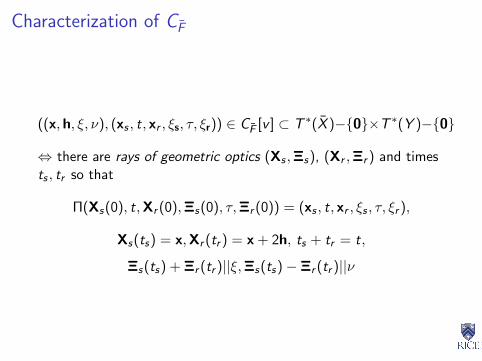
Characterization of CF

((x,h, ξ, ν), (xs , t, xr , ξs, τ, ξr)) ∈ CF [v ] ⊂ T ∗(X )−0×T ∗(Y )−0

⇔ there are rays of geometric optics (Xs ,Ξs), (Xr ,Ξr ) and timests , tr so that

Π(Xs(0), t,Xr (0),Ξs(0), τ,Ξr (0)) = (xs , t, xr , ξs , τ, ξr ),

Xs(ts) = x,Xr (tr ) = x + 2h, ts + tr = t,

Ξs(ts) + Ξr (tr )||ξ,Ξs(ts)− Ξr (tr )||ν

ξ,

Π Π

ξ

(t )r r

(t )r r

s(t )s (t )ss

ss ss(t’ ) (t’ )

r rr (t’ ) (t’ )

t + t = t’ + t’s s r,r,

r

x s, s x r, rp

x

p

kx x k

kxk

Proof

Uses wave equations for u,G and

I Gabor calculus: computes wave front sets of products,pullbacks, integrals, etc. See Duistermaat, Ch. 1.

I Propagation of Singularities Theorem

and that’s all! [No integral representations, phase functions,...]

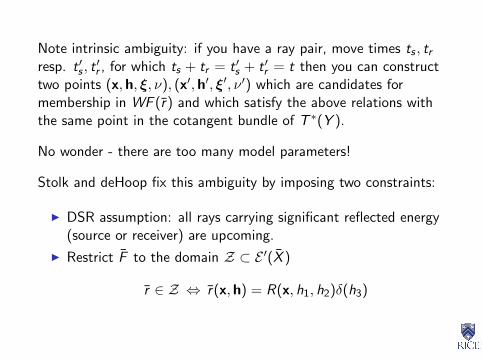
Note intrinsic ambiguity: if you have a ray pair, move times ts , trresp. t ′s , t

′r , for which ts + tr = t ′s + t ′r = t then you can construct

two points (x,h, ξ, ν), (x′,h′, ξ′, ν ′) which are candidates formembership in WF (r) and which satisfy the above relations withthe same point in the cotangent bundle of T ∗(Y ).

No wonder - there are too many model parameters!

Stolk and deHoop fix this ambiguity by imposing two constraints:

I DSR assumption: all rays carrying significant reflected energy(source or receiver) are upcoming.

I Restrict F to the domain Z ⊂ E ′(X )

r ∈ Z ⇔ r(x,h) = R(x, h1, h2)δ(h3)

If r ∈ Z, then (x,h, ξ, ν) ∈WF (r)⇒ h3 = 0. So source andreceiver rays in CF must terminate at same depth, to hit such apoint.

Because of DSR assumption, this fixes the traveltimes ts , tr .

Restricted to Z, CF is injective.

⇒ CF∗F = I

⇒ F ∗F is ΨDO when restricted to Z.

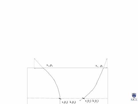
xr(t )

r r(t )

r

s ,p

s(t )s(t )sx s

x r, rx s,,p

k k

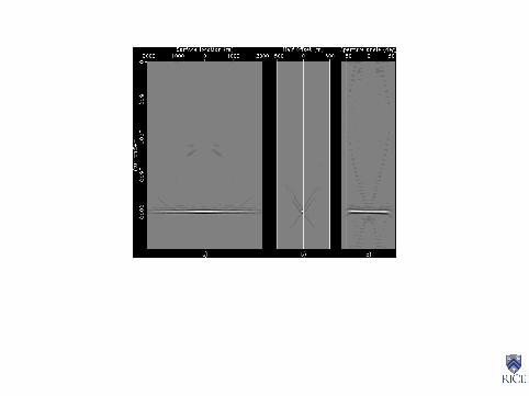
Lens data, shot-geophone migration [B. Biondi, 2002]Left: Image via DSR. Middle: G [v ]d - well-focused (at h = 0), i.e.

in range of χ to extent possible. Right: Angle CIG.

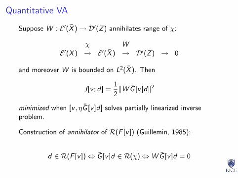
Quantitative VA

Suppose W : E ′(X )→ D′(Z ) annihilates range of χ:

χ WE ′(X ) → E ′(X ) → D′(Z ) → 0

and moreover W is bounded on L2(X ). Then

J[v ; d ] =1

2‖W G [v ]d‖2

minimized when [v , ηG [v ]d ] solves partially linearized inverseproblem.

Construction of annihilator of R(F [v ]) (Guillemin, 1985):

d ∈ R(F [v ])⇔ G [v ]d ∈ R(χ)⇔W G [v ]d = 0

Annihilators, annihilators everywhere...

For Standard Extended Model, several popular choices:

I W = (I −∆)−12∇h (“differential semblance” - WWS, 1986)

I W = I − 1|H|∫

dh (“stack power” - Toldi, 1985)

I W = I − χF [v ]†F [v ] ⇒ minimizing J[v , d ] equivalent to leastsquares.

For Claerbout extension, differential semblance W = h.

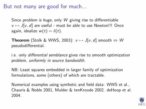
But not many are good for much...

Since problem is huge, only W giving rise to differentiablev 7→ J[v , d ] are useful - must be able to use Newton!!! Onceagain, idealize w(t) = δ(t).

Theorem (Stolk & WWS, 2003): v 7→ J[v , d ] smooth ⇔ Wpseudodifferential.

i.e. only differential semblance gives rise to smooth optimizationproblem, uniformly in source bandwidth.

NB: Least squares embedded in larger family of optimizationformulations, some (others) of which are tractable.

Numerical examples using synthetic and field data: WWS et al.,Chauris & Noble 2001, Mulder & tenKroode 2002. deHoop et al.2004.

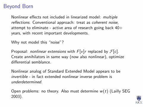
Beyond Born

Nonlinear effects not included in linearized model: multiplereflections. Conventional approach: treat as coherent noise,attempt to eliminate - active area of research going back 40+years, with recent important developments.

Why not model this “noise”?

Proposal: nonlinear extensions with F [v ]r replaced by F [c].Create annihilators in same way (now also nonlinear), optimizedifferential semblance.

Nonlinear analog of Standard Extended Model appears to beinvertible - in fact extended nonlinear inverse problem isunderdetermined.

Open problems: no theory. Also must determine w(t) (Lailly SEG2003).

And so on...

I Elasticity: theory of asymptotic Born inversion at smoothbackground in good shape (Beylkin & Burridge 1988, deHoop& Bleistein 1997). Theory of extensions, annihilators,differential semblance partially complete (Brandsberg-Dahl etal 2003).

I Anisotropy - work of deHoop (Brandsberg-Dahl et al 2003).

I Anelasticity - in the sedimentary section, Q = 100− 1000,lower in gassy sediments and near surface. No mathematicalresults, but some numerics - Minkoff & WWS 1997, Blanch etal 1998.

I Source determination - actually always an issue. Some successin casting as an inverse problem - Minkoff & WWS 1997,Routh et al SEG 2003.

I ...

Selected References

Cohen, J. K. and Bleistein, N.: An inverse method for determiningsmall variations in propagation speed, SIAM J. Appl. Math. 32,1977, pp. 784-799.

Rakesh: A linearized inverse problem for the wave equation,Comm. PDE 13, 1988, pp. 573-601.

Beylkin, G.: Imaging of discontinuities in the inverse scatteringproblem by inversion of a causal generalized Radon transform, J.Math. Phys 26, 1985, pp. 99-108.

Ten Kroode, A. P. E., Smit, D. J., and Verdel, A. R.: A microlocalanalysis of migration Wave Motion 28, 1998, pp. 149-172.

deHoop, M. and Bleistein, N.: Generalized Radon Transforminversions for reflectivity in anisotropic elastic media, InverseProblems 16, 1998, pp. 669-690.

Brandsberg-Dahl, S., De Hoop, M., and Ursin, B.: Focussing indip and AVA compensation on scattering angle/azimuth commonimage gathers, Geophysics 68, 2003, pp. 232-254.

Stolk, C. and Symes, W. W.: Smooth objective functionals forseismic velocity inversion, Inverse Problems 19, 2003, pp. 73-89.

Stolk, C. and Symes, W. W.: Kinematic artifacts in prestack depthmigration, Geophysics 68, May-June 2004.

Minkoff, S. E. and Symes, W. W.: Full waveform inversion ofmarine reflection data in the plane wave domain, Geophysics 62,1997, pp. 540-553.

Grau, G. and Versteeg, R.: The Marmousi Experience: PracticalAspects of Inversion, IFP-Technip, Paris, 1991.

Lions, J. L.: Nonhomogeneous Boundary Value Problems andApplications, Springer Verlag, Berlin, 1972.

Operto, S., Xu, S. and Lambare, G.: Can we image quantitativelycomplex models with rays?, Geophysics 65, 2001, pp. 1223-1238.

Nolan, C. J. and Symes, W. W.: Global solution of a linearizedinverse problem for the wave equation, Comm. PDE 22, 1997, pp.919-952.

Stolk, C.: Microlocal analysis of a seismic linearized inverseproblem, Wave Motion 32, 2000, pp. 267-290.

Stolk, C. and deHoop, M.: Seismic inverse scattering in the waveequation approach, MSRI preprint, 2001.

Hagedoorn, F.: A process of seismic reflection interpretation,Geophysical Prospecting, 1954, pp. 85-127.

Duistermaat, J.: Fourier Integral Operators, Birkhauser, NY, 1996.

Taylor, M.: Pseudodifferential Operators, Princeton UniversityPress, 1981.

Hormander, L.: The Analysis of Linear Partial DifferentialOperators, vols. I-IV, Springer Verlag, 1983.

Nirenberg, L.: Lectures on Partial Differential Equations, CMBSLecture Notes, AMS, 1972.

Treves, F.: Introduction To Pseudodifferential Operators AndFourier Integral Operators, Plenum, 1980.

Claerbout, J.: Basic Earth Imaging (“BEI”) and Imaging theEarth’s Interior (“IEI”), available through SEP web site,sepwww.stanford.edu.

Miller, D., Oristaglio,, M. and Beylkin, G.: A new slant on seismicimaging, Geophysics 52, pp. 943-964, 1987.

Bleistein, N., Cohen, J. and Stockwell, J.: The Mathematics ofSeismic Imaging, Migration, and Inversion, Springer, 2000.

Dobrin, M. and Savit, C.: Introduction to Geophysical Prospecting

Yilmaz, O.: Seismic Data Processing, 2nd edtion, SEG, 1999.

Symes, W.: Mathematics of Reflection Seismology, Lecture Notes,www.trip.caam.rice.edu, 1995.

Symes, W.: 2002 CIME Notes, www.trip.caam.rice.edu.