C H A P T E R 16

Mathematics after Calculus

I would like this book to do more than help you pass calculus. (I hope it does that too.) After calculus you will have choices- Which mathematics course to take next?- and these pages aim to serve as a guide. Part of the answer depends on where you are going-toward engineering or management or teaching or science or another career where mathematics plays a part. The rest of the answer depends on where the courses are going. This chapter can be a useful reference, to give a clearer idea than course titles can do:

Linear Algebra Differential Equations Discrete Mathematics

Advanced Calculus (with Fourier Series) Numerical Methods Statistics

Pure mathematics is often divided into analysis and algebra and geometry. Those parts come together in the "mathematical way of thinking9'-a mixture of logic and ideas. It is a deep and creative subject-here we make a start.

Two main courses after calculus are linear algebra and differential equations. I hope you can take both. To help you later, Sections 16.1 and 16.2 organize them by examples. First a few words to compare and contrast those two subjects.

Linear algebra is about systems of equations. There are n variables to solve for. A change in one affects the others. They can be prices or velocities or currents or concentrations-outputs from any model with interconnected parts.

Linear algebra makes only one assumption-the model must be linear. A change in one variable produces proportional changes in all variables. Practically every subject begins that way. (When it becomes nonlinear, we solve by a sequence of linear equations. Linear programming is nonlinear because we require x >, 0.)Elsewhere J wrote that "Linear algebra has become as basic and as applicable as calculus, and fortunately it is easier." I recommend taking it.

A differential equation is continuous (from calculus), where a matrix equation is discrete (from algebra). The rate dyldt is determined by the present state y-which changes by following that rule. Section 16.2 solves y' = cy + s(t) for economics and life sciences, and y" + by' + cy =f(t) for physics and engineering. Please keep it and refer to it.

16 Mathematics after Calculus

A third key direction is discrete mathematics. Matrices are a part, networks and algorithms are a bigger part. Derivatives are not a part-this is closer to algebra. It is needed in computer science. Some people have a knack for counting the ways a computer can send ten messages in parallel-and for finding the fastest way.

Typical question: Can 25 states be matched with 25 neighbors, so one state in each pair has an even number of letters? New York can pair with New Jersey, Texas with Oklahoma, California with Arizona. We need rules for Hawaii and Alaska. This matching question doesn't sound mathematical, but it is.

Section 16.3 selects four topics from discrete mathematics, so you can decide if you want more.

Go back for a moment to calculus and differential equations. A completely realistic problem is seldom easy, but we can solve models. (Developing a good model is a skill in itself.) One method of solution involves complex numbers:

any function u(x + iy) solves uxx+ u,, = 0 (Laplace equation)

any function eik("+") solves u,, - c2uxx= 0 (wave equation).

From those building blocks we assemble solutions. For the wave equation, a signal starts at t = 0.It is a combination of pure oscillations eikx.The coefficients in that combination make up the Fourier transform-to tell how much of each frequency is in the signal. A lot of engineers and scientists would rather know those Fourier coefficients than f(x).

A Fourier series breaks the signal into Z a, cos kx or Z b, sin kx or T. ekeikx. These sums can be infinite (like power series). Instead of values of f(x), or derivatives at the basepoint, the function is described by a,, b,, c,. Everything is computed by the "Fast Fourier Transform." This is the greatest algorithm since Newton's method.

A radio signal is near one frequency. A step function has many frequencies. A delta function has every frequency in the same amount: 6(x) = Z cos kx. Channel 4 can't broadcast a perfect step function. You wouldn't want to hear a delta function.

We mentioned computing. For nonlinear equations this means Newton's method. For Ax = b it means elimination-algorithms take the place of formulas. Exact solu- tions are gone-speed and accuracy and stability become essential. It seems right to make scientific computing a part of applied mathematics, and teach the algorithms with the theory. My text Introduction to Applied Mathematics is one step in this direction, trying to present advanced calculus as it is actually used.

We cannot discuss applications and forget statistics. Our society produces oceans of data-somebody has to draw conclusions. To decide if a new drug works, and if oil spills are common or rare, and how often to have a checkup, we can't just guess. I am astounded that the connection between smoking and health was hidden for centuries. It was in the data! Eventually the statisticians uncovered it. Professionals can find patterns, and the rest of us can understand (with a little mathematics) what has been found.

One purpose in studying mathematics is to know more about your own life. Calculus lights up a key idea: Functions. Shapes and populations and heart signals and profits and growth rates, all are given by functions. They change in time. They have integrals and derivatives. To understand and use them is a challenge-mathematics takes effort. A lot of people have contributed, in whatever way they could-as you and I are doing. We may not be Newton or Leibniz or Gauss or Einstein, but we can share some part of what they created.

599 16.1 Vector Spaces and Llnear Algebra

16.1 Vector Spaces and Linear Algebra

You have met the idea of a matrix. An m by n matrix A has m rows and n columns (it is square if m =n). It multiplies a vector x that has n components. The result is a vector Ax with m components. The central problem of linear algebra is to go back- ward: From Ax =bfind x. That is possible when A is square and invertible. Otherwise there is no solution x-or there are infinitely many.

The crucial property of matrix multiplication is linearity. If Ax = b and AX = B then A times x + X is b + B. Also A times 2x is 2b. In general A times cx is cb. In particular A times 0 is 0 (one vector has n zeros, the other vector has m zeros). The

. whole subject develops from linearity. Derivatives and integrals obey linearity too.

Question 1 What are the solutions to Ax =O? One solution is x =0. There may be other solutions and they fill up the "nullspace":

x = 2 x = o 011requires 1 =[J also allows y = - 1 y = o

z z = 3 L A

When there are more unknowns than equations-when A has more columns than rows-the system Ax =0 has many solutions. They are not scattered randomly around! Another solution is X =4, Y= -2, Z =6. This lies on the same line as (2, -1,3) and (0,0,O). Always the solutions to Ax =0 form a "space" of vectors- which brings us to a central idea of linear algebra.

Note These pages are not concentrating on the mechanics of multiplying or invert- ing matrices. Those are explained in all courses. My own teaching emphasizes that Ax is a combination of the columns of A. The solution x = A-'b is computed by elimination. Here we explain the deeper idea of a vector space-and especially the particular spaces that control Ax =6. I cannot go into the same detail as in my book on Linear Algebra and Its Applications, where examples and exercises develop the new ideas. Still these pages can be a useful support.

All vectors with n components lie in n-dimensional space. You can add them and subtract them and multiply them by any c. (Don't multiply two vectors and never write llx or 1/A). The results x + X and x -X and cx are still vectors in the space. Here is the important point:

The line of solutions to Ax =0 is a "subspace"-a vector space in its own right. The sum x + X has components 6, -3,9-which is another solution. The difference x -X is a solution, and so is 4x. These operations leave us in the subspace.

The nullspace consists of all solutions to Ax = 0. It may contain only the zero vector (as in the first example). It may contain a line of vectors (as in the second example). It may contain a whole plane of vectors (Problem 5). In every case x + X and x -X and cx are also in the nullspace. We are assigning a new word to an old idea-the equation x - 2y =0 has always been represented by a line (its nullspace). Now we have 6-dimensional subspaces of an %dimensional vector space.

Notice that x2 - y =0 does not produce a subspace (a parabola instead). Even the x and y axes together, from xy = 0, do not form a subspace. We go off the axes when we add (1,O) to (0, 1). You might expect the straight line x - 2y = 1 to be a subspace, but again it is not so. When x and y are doubled, we have X - 2Y =2. Then (X, Y) is on a different line. Only Ax = 0 is guaranteed to produce a subspace.

16 Mathematics after Calculus

Figure 16.1 shows the nullspace and "row space." Check dot products (both zero).

Fig. 16.1 The nullspace is perpendicular to the rows of A (the columns of AT).

Question 2 When A multiplies a vector x, what subspace does Ax lie in? The product Ax is a combination of the columns of A-hence the name "column space":

No choice of x can produce Ax = (0,0, 1). For this A, all combinations of the columns end in a . The column space is like the xy plane within xyz space. It is a subspace of m-dimensional space, containing every vector b that is a combination of the columns:

The system Ax = b has a solution exactly when b is in the column space.

When A has an inverse, the column space is the whole n-dimensional space. The nullspace contains only x = 0. There is exactly one solution x = A 1 b . This is the good case-and we outline four more key topics in linear algebra.

1. Basis and dimension of a subspace. A one-dimensional subspace is a line. A plane has dimension two. The nullspace above contained all multiples of (2, -1, 3)-by knowing that "basis vector" we know the whole line. The column space was a plane containing column 1 and column 2. Again those vectors are a "basis"-by knowing the columns we know the whole column space.

Our 2 by 3 matrix has three columns: (1,O) and (2, 3) and (0, 1). Those are not a basis for the column space! This space is only a plane, and three vectors are too many. The dimension is two. By combining (1,O) and (0, 1) we can produce the other vector (2, 3). There are only two independent columns, and they form a basis for this column space.

In general: When a subspace contains r independent vectors, and no more, those vectors are a basis and the dimension is r. "Independent" means that no vector is a combination of the others. In the example, (1,O) and (2, 3) are also a basis. A subspace has many bases, just as a plane has many axes.

2. Least squares. If Ax = b has no solution, we look for the x that comes closest. Section 1 1.4 found the straight line nearest to a set of points. We make the length of Ax - b as small as possible, when zero length is not possible. No vector solves

16.1 Vector Spaces and Llnear Algebra

Ax = b, when b is not in the column space. So b is projected onto that space. This leads to the "normal equations" that produce the best x:

When a rectangular matrix appears in applications, its transpose generally comes too. The columns of A are the rows of AT. The rows of A are the columns of AT. Then AT^ is square and symmetric-equal to its transpose and vital for applied mathematics.

3. Eigenvalues (for square matrices only). Normally Ax points in a direction different from x. For certain special eigenvectors, Ax is parallel to x. Here is a 2 by 2 matrix with two eigenvectors-in one case Ax = 5x and in the other Ax = 2x;

3 2 1

Ax=Ax: [ 1 4 ][]=[:]=5[:] 1 and [: :][-:]=[-:]=2[-:].

The multipliers 5 and 2 are the eigenvalues of A. An 8 by 8 matrix has eight eigen- values, which tell what the matrix is doing (to the eigenvectors). The eigenvectors are uncoupled, and they go their own way. A system of equations dyldt = Ay acts like one equation-when y is an eigenvector:

d ~ i l d t = 3 ~ 1 + 2 ~ 2 yl = eSt has the solution which is est

dyddt = yi + 4 ~ 2 y2 = eSt [:I.

The eigenvector is (1, 1). The eigenvalue A = 5 is in the exponent. When you substitute y1 and y2 the differential equations become 5est = 5est. The fundamental principle for dyldt = cy still works for the system dyldt = Ay: Look for pure exponential solu- tions. The eigenvalue "lambda" is the growth rate in the exponent.

I have to add: Find the eigenvectors also. The second eigenvector (2, - 1) has eigenvalue i = 2. A second solution is y1 = 2e2', y2 = - e". Substitute those into the equation-they are even better at displaying the general rule:

If Ax = Ax then d/dt(ehx) = ~ ( e ~ ~ x ) . The pure exponentials are y = eAtx.

The four entries of A pull together for the eigenvector. So do the 64 entries of an 8 by 8 matrix-again e"x solves the equation. Growth or decay is decided by A > 0 or K < 0. When A = k + iw is a complex number, growth and oscillation combine in e ~ t = e k t e i ~ t = ekt(cos wt + i sin at).

Subspaces govern static problems Ax = b. Eigenvalues and eigenvectors govern dynamic problems dyldt = Ay. Look for exponentials y = eUx.

4. Determinants and inverse matrices. A 2 by 2 matrix has determinant D = ad - bc. This matrix has no inverse if D = 0. Reason: A-' divides by D:

This pattern extends to n by n matrices, but D and A - l become more 'complicated. For 3 by 3 matrices D has six terms. Section 11.5 identified D as a triple product

a (b x c) of the columns. Three events come together in the singular case: D is zero and A has no inverse and the columns lie in a plane. The opposite events produce the "nonsingular" case: D is nonzero and A- ' exists. Then Ax = b is solved by x = A- b.

16 Mathematics after Calculus

D is also the product of the pivots and the product of the eigenvalues. The pivots arise in elimination-the practical way to solve Ax = b without A- ' . To find eigen- values we turn Ax = Ax into ( A- i1)x = 0 . By a nice twist of fate, this matrix A -A1 has D = 0.Go back to the example:

[f : ] - A [ : : ] = [ j ; ' 4 iA]has D = ( i - q ( 4 - A ) - 2 = A 2 - 7 A l O .

The equation A2 - 71. + 10 = 0 gives 1. = 5 and A = 2. The eigenvalues come first, to make D = 0.Then ( A- 51)x = 0 and (A - 2I)x = 0 yield the eigenvectors. These x's go into y = e"x to solve differential equations-which come next.

16.1

Read-through questions

If Ax = b and AX = B, then A times 2x + 3X equals a . If Ax = 0 and AX = 0 then A times 2x + 3X equals b . In this case x and X are in the c of A, and so is the combination d . The nullspace contains all solutions to

e . It is a subspace, which means f . If x = (1, 1, 1) is in the nullspace then the columns add to g , so they are (independent)(dependent).

Another subspace is the h space of A, containing all combinations of the columns. The system Ax = b can be solved when b is i . Otherwise the best solution comes from A T ~ x= i . Here AT is the k matrix, whose rows are I . The nullspace of AT contains all solutions to

m . The n space of AT (row space of A) is the fourth fundamental subspace. Each su bspace has a basis containing as many o vectors as possible. The number of vectors in the basis is the P of the subspace.

When Ax =Ax, the number ;I. is an q and x is an r . The equation dyldt = A y has the exponential solution

y = s . A 7 by 7 matrix has t eigenvalues, whose product is the u D. If D is nonzero the matrix A has an

v . Then Ax = b is solved by x = w . The formula for D contains 7! = 5040 terms, so x is better computed by

x . On the other hand Ax = i.x means that A ->.I has determinant v . The eigenvalue is computed before the

Z .

Find the nullspace in 1-6. Along with x go all cx.

12 - 6 1 A = 2 ] (solve Ax = 0)

2 4 ' = [ - 6 3 1

1 0 1 0 1

3 C = 0 1 (solve C x = 0)

1 2 cT=[o1 2 1

EXERCISES

7 Change Problem 1 to Ax = (a) Find any particular r:1L A

solution x,. (b) Add any x , from the nullspace and show that x , + xo is also a solution.

8 Change Problem 1 to Ax = Ll and find all solutions. L

Graph the lines x , + 2x2 = 1 and 2 x , + 4x2 = 0 in a plane.

9 Suppose AX, = b and Ax, = 0 . Then by linearity &P + xo) = -. Conclusion: The sum of a particular solution x , and any nullvector xo is .

10 Suppose Ax = b and AX, = b. Then by linearity A(x -x,) = . The difference between solutions is a vector in . Conclusion: Every solution has the form x = x , + xo , one particular solution plus a vector in the nullspace.

11 Find three vectors b in the column space of E. Find all vectors b for which Ex = b can be solved.

12 If Ax = 0 then the rows of A are perpendicular to x . Draw the row space and nullspace (lines in a plane) for A above.

13 Compute CCT and CTC.Why not C2?

14 Show that C x = b has no solution, if b = (-1, 1,l). Find the best solution from C T C X = cTb.

15 CT has three columns. How many are independent? Which ones?

16 Find two independent vectors that are in the column space of C but are not columns of C.

17 For which of the matrices A B C E F are the columns a basis for the column space?

603 16.2 Differential Equations

18 Explain the reasoning: If the columns of a matrix A are 27 Compute the determinant of E -AI. Find all A's that make independent, the only solution to Ax =0 is x =0. this determinant zero. Which eigenvalue is repeated?

19 Which of the matrices ABCEF have nonzero deter- 28 Which previous problem found eigenvectors for Ex =Ox? minants? Find an eigenvector for Ex =3x.

20 Find a basis for the full three-dimensional space using 29 Find the eigenvalues and eigenvectors of A. only vectors with positive components. 30 Explain the reasoning: A matrix has a zero eigenvalue if

and only if its determinant is zero. 21 Find the matrix F - ' for which FF - '=I =[:;I- 31 Find the matrix H whose eigenvalues are 0 and 4 with

eigenvectors (1, 1)and (1, -1). 22 Verify that (determinant of F ) ~ =(determinant of F ~ ) . 32 If Fx =I x then multiplying both sides by gives

23 (Important) Write down F -AI and compute its determi- F-'x =A-'x. If F has eigenvalues 1 and 3 then F- ' has . The determinants of F and F arenant. Find the two numbers A that make this determinant eigenvalues

zero. For those two numbers find eigenvectors x such that Fx =Ax. 33 True or false, with a reason or an example.

24 Compute G =F 2. Find the determinant of G -AI and the (a) The solutions to Ax =b form a subspace. two A's that make it zero. For those I's find eigenvectors x [:Isuch that Gx =Ax. Conclusion: if Fx =Ax then F ~ X=A2x. (b) [ O 2] has in its nullspace and column space.

0 0 25 From Problem 23 find two exponential solutions to the (c) ATA has the same entry in its upper right and lower equation dyldt =Fy. Then find a combination of those left corners. solutions that starts from yo =(1,O) at t =0. (d)If Ax =Ax then y =e" solves dyldt =Ay. 26 From Problem 24 find two solutions to dyldt = Gy. Then (e) If the columns of A are not independent, their combi- find the solution that starts from yo =(2, 1). nations still form a subspace.

16.2 Differential Equations

We just solved differential equations by linear algebra. Those were special systems dyJdt= Ay, linear with constant coefficients. The solutions were exponentials, involving eU. The eigenvalues of A were the "growth factors" A. This section solves other equations-by no means all. We concentrate on a few that have important applications.

Return for a moment to the beginning-when direct integration was king:

In 1, y(t) is the integral of s(t). In 2, y(t) is the integral of cy(t). That sounds circular- it only made sense after the discovery of y = ec'. This exponential has the correct derivative cy. To find it by integration instead of inventing it, separate y from t:

Separation and integration also solve 3:j dy/u(y)=5 c(t)dt.The model logistic equation has u = y - y2 = quadratic. Equation 2 has u = y = linear. Equation 1is also a special case with u = 1 = constant. But 2 and 1are very different, for the following reason.

The compound interest equation y' = cy is growing from inside. The equation y' = s(t) is growing from outside. Where c is a "growth rate," s is a "source." They don't have the same meaning, and they don't have the same units. The combination y' =cy + s was solved in Chapter 6, provided c and s are constant-but applications force us to go further.

--

16 Mathematics after Calculus

In three examples we introduce non-constant source terms.

EXAMPLE 1 Solve dyldt = cy + s with the new source term s = ekt.

Method Substitute y = B@, with an "undetermined coefficient" B to make it right:

kBek' = cBek' + ekt yields B = l / (k- c).

The source ek' is the driving term. The solution Bekt is the response. The exponent is the same! The key idea is to expect ek' in the response.

Initial condition To match yo at t = 0, the solution needs another exponential. It is the free response Aec', which satisfies dyldt = cy with no source. To make y = Aec' + Bek' agree with yo, choose A = yo - B:

Final solution y = (yo- B)ec' + Bekt = yoect+ (ek' - ec')/(k- c). (1)

Exceptional case B = l / ( k- c) grows larger as k approaches c. When k = c the method breaks down-the response Bek' is no longer correct. The solution (1) approaches 010, and in the limit we get a derivative. It has an extra factor t:

ekt - ect - change in ect

+ -d

(ect)= tect. k - c change in c dc

The correct response is tectwhen k = c. This is the form to substitute, when the driving rate k equals the natural rate c (called resonance).

Add the free response yoec' to match the initial condition.

EXAMPLE 2 Solve dyldt = cy + s with the new source term s = cos kt.

Substitute y = B sin kt + D cos kt. This has two undetermined coefficients B and D:

kB cos kt - kD sin kt = c(B sin kt + D cos kt)+ cos kt. (3)

Matching cosines gives kB = cD + 1. The sines give -kD = cB. Algebra gives B, D, y:

c sin kt + k cos ktB=- C D=- k y= k2+c2 (4)k2 + c2 k2 + c2

Question Why do we need both B sin kt and D cos kt in the response to cos kt?

First Answer Equation (3)is impossible if we leave out B or D. Second Answer cos kt is f eikt+ i e -"'. So eiktand e-"' are both in the response.

EXAMPLE 3 Solve dyldt = cy + s with the new source term s = tekt.

Method Look for y = ~ e ~ '+ Dtek'. Problem 13 determines B and D. Add Aec' as needed, to match the initial value yo.

SECOND-ORDER EQUATIONS

The equation dyldt = cy is jrst-order. The equation d2y/dt2= - cy is second-order. The first is typical of problems in life sciences and economics-the rate dyldt depends on the present situation y. The second is typical of engineering and physical sciences- the acceleration d2y/dt2enters the equation.

If you put money in a bank, it starts growing immediately. If you turn the wheels of a car, it changes direction gradually. The path is a curve, not a sharp corner. Newton's law is F = ma, not F = mu.

16.2 Differential Equations

A mathematician compares a straight line to a parabola. The straight line crosses the x axis no more than once. The parabola can cross twice. The equation ax2+ bx + c = 0 has two solutions, provided we allow them to be complex or equal. These are exactly the possibilities we face below: two real solutions, two complex solutions, or one solution that counts twice. The quadratic could be x2 - 1 or x2 + 1 or x2. The roots are 1 and -1, i and - i, 0 and 0.

In solving diflerential equations the roots appear in the exponent, and are called A.

EXAMPLE 4 y" = +y: solutions y = et and y = e-' A = 1, -1 EXAMPLE 5 y" = 0 y: solutions y = 1 and y = t iZ = 0,0 EXAMPLE 6 y" = -y: solutions y = cos t and y = sin t A = i, - i

Where are the complex solutions? They are hidden in Example 6, which could be written y = eit and y = e-". These satisfy y" = -y since i2 = - 1. The use of sines and cosines avoids the imaginary number i, but it breaks the pattern of e".

Example 5 also seems to break the pattern-again eU is hidden. The solution y = 1 is eO'. The other solution y = t is teot. The zero exponent is repeated-another excep-tional case that needs an extra factor t.

Exponentials solve every equation with constant coeficients and zero right hand side:

To solve ay" + by' + cy = 0 substitute y = e" and find A.

This method has three steps, leading to the right exponents A = r and A = s:

1. With y = eU the equation is aA2ee" + bAe" + ceAt= 0. Cancel e". 2. Solve aA2 + bA + c = 0. Factor or use the formula A = (- b f Jbi-rlac)/2a. 3. Call those roots A = r and A= s. The complete solution is y = Aert+ Best.

The pure exponentials are y = er' and y = e". Depending on r and s, they grow or decay or oscillate. They are combined with constants A and B to match the two conditions at t = 0. The initial state yo equals A + B. The initial velocity yb equals rA + sB (the derivative at t = 0).

EXAMPLE 7 Solve y" - 3y' + 2y = 0 with yo = 5 and yb = 4.

Step 1 substitutes y = e". The equation becomes i2e" - 3Ae" + 2e" = 0. Cancel e". Step 2 solves 1.' -31. + 2 = 0. Factor into (A -1)(A-2) = 0. The exponents r, s are 1,2. Step 3 produces y = Aet + ~ e ~ ' .The initial conditions give A + B = 5 and 1 A + 2B = 4. The constants are A = 6 and B = - 1. The solution is y = 6et - elt.

This solution grows because there is a positive A. The equation is "unstable." It becomes stable when the middle term -3y' is changed to + 3y'. When the damping is positive the solution decays. The 1's are negative:

EXAMPLE 8 (A2+ 31 + 2) factors into (1 + 1)(1+ 2). The exponents are -1 and -2. The solution is y = Ae-' + Be-2t. It decays to zero for any initial condition.

EXAMPLES 9-10 Solve y" + 2y' + 2y = 0 and y" + 2y' + y = 0. How do they differ?

Key difference A2 + 2A + 2 has complex roots, L2 + 23, + 1 has a repeated root:

A 2 + 2 1 + 2 = 0 gives A = - 1 + i ( 1 + 1 ) ~ = 0 gives A=-1, -1 .

The -1 in all these R's means decay. The i means oscillation. The first exponential is e(-I+ i)t ,which splits into e-' (decay) times eit (oscillation). Even better, change eit

16 Mathematics after Calculus

and e-" into cosines and sines: = Ae(-1 +i)t + ge(-1- i ) t = e-'(a cos t + b sin t). ( 5 )

At t = 0 this produces yo = a. Then matching yb leads to b. Example 10 has r = s = - 1 (repeated root). One solution is e-' as usual. The

second solution cannot be another e-'. Problem 21 shows that it is te-'-again the exceptional case multiplies by t! The general solution is y = Ae-' + Bte-'.

Without the damping term 2yf, these examples are y" + 2y = 0 or y" + y = 0-pure oscillation. A small amount of damping mixes oscillation and decay. Large damping gives pure decay. The borderline is when A is repeated (r = s). That occurs when b2 -4ac in the square root is zero. The borderline between two real roots and two complex roots is two repeated roots.

The method of solution comes down to one idea: Substitute y = eU. The equations apply to mechanical vibrations and electrical circuits (also other things, but those two are of prime importance). While describing these applications I will collect the information that comes from A.

SPRINGS AND CIRCUITS: MECHANICAL AND ELECTRICAL ENGINEERING

A mass is hanging from a spring. We pull it down an extra distance yo and give it a starting velocity yb. The mass moves up or down, obeying Newton's law: mass times acceleration equals spring force p lus damping force:

my" = - ky - dy' or my" + dy' + ky = 0. (6)

This is free oscillation. The spring force -ky is proportional to the stretching y (Hooke's law). The damping acts like a shock absorber or air resistance-it takes out energy. Whether the system goes directly toward zero or swings back and forth is decided by the three numbers m, d, k. They were previously called a, b, c.

16A The solutions e" to my" + dy' + ky = 0 are controlled by the roots of mA2 + d l + k = 0. With d > 0 there is damping and decay. From J62-4mk there may be oscillation:

overdamping: d > 4mk gives real roots and pure decay (Example 8)

underdamping: d < 4mk gives complex roots and oscillation (Example 9)

I critical damping: d2 = 4mk gives a real repeated root -d/2m (Example 10)

We are using letters when the examples had numbers, but the results are the same:

d lm i 2 + d 1 + k = 0 hasroots r , s = - - f --,/;iT-4mk.

2m 2m

Overdamping has no imaginary parts or oscillations: y = Ae" + Bes'. Critical damping has r = s and an exceptional solution with an extra t: y = Ae" + Bte". (This is only a solution when r = s.) Underdamping has decay from -d/2m and oscillation from the imaginary part. An undamped spring (d = 0) has pure oscillation at the natural fre- quency wo = Jklm.

AN these possibilities are in Figure 16.2, created by Alar Toomre. At the top is pure oscillation (d = 0 and y = cos 2t). The equation is y" + dy' + 4y = 0 and d starts to grow. When d reaches 4, the quadratic is A2 + 41 + 4 or (1 + 2)2. The repeated root

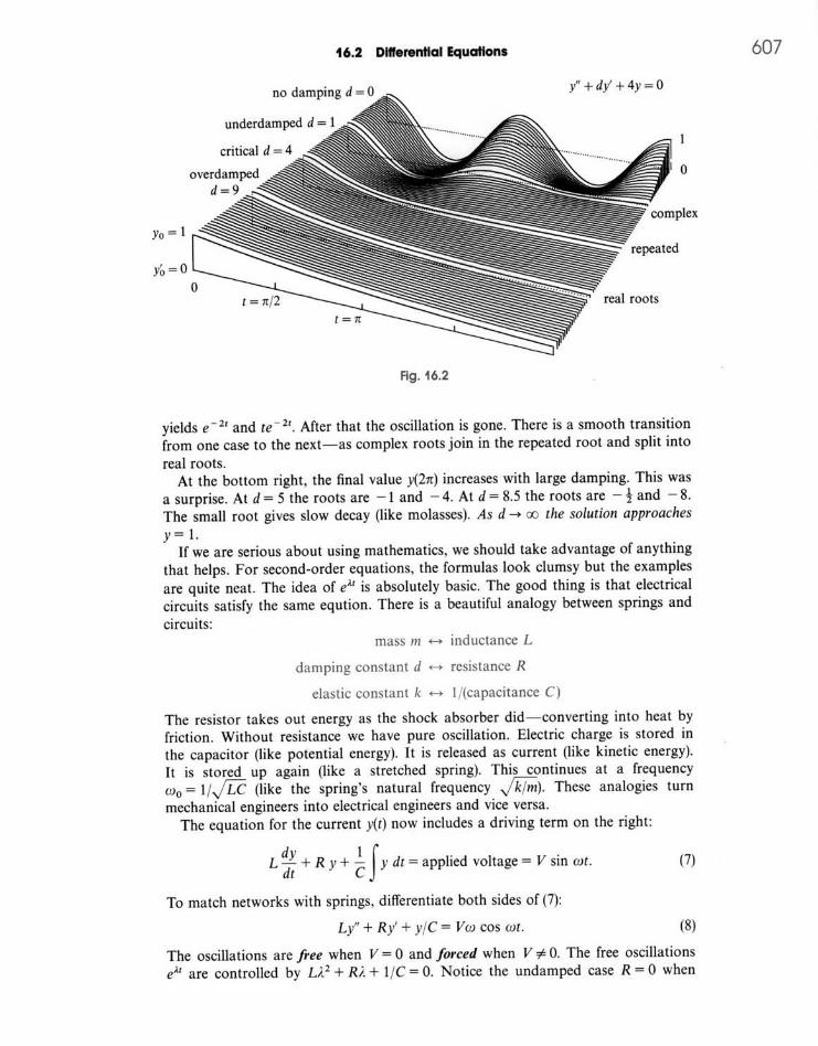
16.2 Differential Equations 6

1

0

)lex

yo = 1

yo,= 0

Fig. 16.2

yields e-2t and te-2t. After that the oscillation is gone. There is a smooth transition

from one case to the next-as complex roots join in the repeated root and split intoreal roots.

At the bottom right, the final value y(27n) increases with large damping. This wasa surprise. At d = 5 the roots are -1 and - 4. At d = 8.5 the roots are - ' and - 8.

The small root gives slow decay (like molasses). As d -+ oo the solution approaches

y= 1.If we are serious about using mathematics, we should take advantage of anything

that helps. For second-order equations, the formulas look clumsy but the examplesare quite neat. The idea of e"' is absolutely basic. The good thing is that electricalcircuits satisfy the same eqution. There is a beautiful analogy between springs andcircuits:

mass m , inductance L

damping constant d *- resistance R

elastic constant k - 1/(capacitance C)

The resistor takes out energy as the shock absorber did-converting into heat byfriction. Without resistance we have pure oscillation. Electric charge is stored inthe capacitor (like potential energy). It is released as current (like kinetic energy).It is stored up again (like a stretched spring). This continues at a frequencyc0 = 1/-LC (like the spring's natural frequency k/r). These analogies turn

mechanical engineers into electrical engineers and vice versa.The equation for the current y(t) now includes a driving term on the right:

L dt + R y + -C y dt = applied voltage = V sin cot. (7)

To match networks with springs, differentiate both sides of (7):

Ly" + Ry' + y/C = Vwt cos cot. (8)

The oscillations are free when V = 0 and forced when V A 0. The free oscillationseAt are controlled by LA2 + RA + 1/C = 0. Notice the undamped case R = 0 when

07

16 Mathematics after Calculus

A = i/-. This shows the natural frequency w, = l / p . Damped free oscilla- tions are in the exercises-what is new and important is the forcing from the right hand side. Our last step is to solve equation (8).

PARTICULAR SOLUTIONS-THE METHOD OF UNDETERMINED COEFFICIENTS

The forcing term is a multiple of cos wt. The "particular solution" is a multiple of cos o t plus a multble of sin wt. To discover the undetermined coefficients in y = a cos cot + b sin cot, substitute into the differential equation (8):

-Lw2(a cos wt + b sin ot) + Rw(- a sin wt + b cos wt)

+ (a cos wt + b sin wt)/C = Vw cos wt.

The terms in cos wt and the terms in sin o t give two equations for a and b:

-a h 2+ bRw + a/C = Vw and -b ~ w ~- aRw + blC = 0. (9)

EXAMPLE 11 Solve y" + y = cos o t . The oscillations are forced at frequency w. The oscillations are free (y" + y = 0) at frequency 1. The solution contains both.

Particular solution Set y = a cos o t + b sin wt at the driving frequency w, and (9) becomes

- a w 2 + O + a = 1 and -bo2-O+b=O.

The second equation gives b = 0. No sines are needed because the problem has no dyldt. The first equation gives a = 1/(1-w2), which multiplies the cosine:

y = (cos wt)/(1 -w2) solves y" + y = cos wt. (10)

General solution Add to this particular solution any solution to y" + y = 0:

Problem of resonance When the driving frequency is o = 1, the solution (1 1) becomes meaningless-its denominator is zero. Reason: The natural frequency in cos t and sin t is also 1. A new particular solution comes from t cos t and t sin t.

The key to success is to know the form for y. The table displays four right hand sides and the correct y's for any constant-coefficient equation:

Right hand side Particular solution ekt y = Bek' (same exponent) cos wt or sin o t y = a cos a t + b sin wt (include both) polynomial in t y = polynomial of the same degree ektcos wt or ekt sin wt y = aekt cos wt + bekt sin wt

Exception If one of the roots A for free oscillation equals k or ico or 0 or k + iw, the corresponding y in the table is wrong. The proposed solution would give zero on the right hand side. The correct form for y includes an extra t. All particular solutions are computed by substituting into the differential equation.

Apology Constant-coefficient equations hardly use calculus (only e"). They reduce directly to algebra (substitute y, solve for iland a and b). I find the S-curve from the logistic equation much more remarkable. The nonlinearity of epidemics or heartbeats or earthquakes demands all the calculus we know. The solution is not so predictable. The extreme of unpredictability came when Lorenz studied weather prediction and discovered chaos.

NUMERICAL METHODS

Those four pages explained how to solve linear equations with constant coefficients: Substitute y = eat. The list of special solutions becomes longer in a course on differential equations. But for most nonlinear problems we enter another world- where solutions are numerical and approximate, not exact.

In actual practice, numerical methods for dyldt =f (t, y) divide in two groups:

1. Single-step methods like Euler and Runge-Kutta 2. Multistep methods like Adams-Bashforth

The unknown y and the right side f can be vectors with n components. The notation stays the same: the step is At = h, the time t, is nh, and y, is the approximation to the true y at that time. We test the first step, to find y, from yo = 1. The equation is dyldt = y, so the right side is f = y and the true solution is y = et.

Notice how the first value off (in this case 1) is used inside the second f:

TEST y, = 1 + +h[l+ (1 + h)] = 1 + h + $h2

At time h the true solution equals eh. Its infinite series is correct through h2 for Improved Euler (a second-order method). The ordinary Euler method yn+ = yn+ hf (t,, y,) is first-order. TEST: y, = 1+ h. Now try Runge-Kutta (a fourth-order method):

Now the first value off is used in the second (for k,), the second is used in the third, and then k3 is used in k,. The programming is easy. Check the accuracy with another test on dyldt = y:

h2 h3 h4 =1+ h + -+ -+ -. This answer agrees with eh through h4.

2 6 24

These formulas are included in the book so that you can apply them directly- for example to see the S-shape from the logistic equation with f= cy - by2.

Multistep formulas are simpler and quicker, but they need a single-step method to get started. Here is y, in a fourth-order formula that needs yo, y,, y,, y,. Just shift all indices for y,, y,, and y, + ,:

h Multistep y4 = y3 + -[55yi - 59y; + 37y; - 9ybl.

24

The advantage is that each step needs only one new evaluation of y; =f(t,, y,). Runge-Kutta needs four evaluations for the same accuracy.

Stability is the key requirement for any method. Now the good test is y' = -y. The solution should decay and not blow up. Section 6.6 showed how a large time step makes Euler's method unstable-the same will happen for more accurate formulas. The price of total stability is an "implicit method" like y, = yo + + h ( ~ b+ y;), where the unknown y, appears also in y; . There is an equation to be solved at every step. Calculus is ending as it started-with the methods of Isaac Newton.

16 Mathematics after Calculus

16.2 EXERCISES

Read-through questions

The solution to y' -5y = 10 is y = Ae5t + B. The homo-geneous part Ae 5' satisfies y'-5y = a . The particu-lar solution B equals b . The initial condition Yo ismatched by A = c . For y'-5y = ekt the right formis y =Ae + d . For y'-5y = cos t the form isy = Ae5'+ e + f

The equation y"+4y'+ 5y=0 is second-order becauseg . The pure exponential solutions come from the roots

of h , which are r= i and s= I . The generalsolution is y = k . Changing 4y' to I yields pureoscillation. Changing to 2y' yields = - 1 + 2i, when thesolutions become y= m . This oscillation is(over)(under)(critically) damped. A spring with m = 1, d = 2,k = 5 goes (back and forth)(directly to zero). An electricalnetwork with L = 1, R = 2, C = also n

One particular solution of y" + 4y = e' is e' timeso . If the right side is cos t, the form of y, is p . If the

right side is 1 then y, = q . If the right side is r wehave resonance and y, contains an extra factor s

Problems 1-14 are about first-order linear equations.

I Substitute y = Be3 ' into y' - y = 8e3' to find a particularsolution.

2 Substitute y = a cos 2t + b sin 2t into y' + y = 4 sin 2t tofind a particular solution.

3 Substitute y = a + bt + ct2 into y' + y = 1 + t2 to find aparticular solution.

4 Substitute y = aetcos t + be'sin t into y' = 2e'cos t to finda particular solution.

5 In Problem 1 we can add Ae' because this solves the equa-tion . Choose A so that y(0) = 7.

6 In Problem 2 we can add Ae - t, which solvesChoose A to match y(0)= 0.

7 In Problem 3 we add to match y(O)= 2.

8 In Problem 4 we can add y = A. Why?

9 Starting from Yo= 0 solve y' = ek ' and also solve y' = 1.Show that the first solution approaches the second as k -0.

10 Solve y' - y = ek' starting from Yo= 0. What happens toyour formula as k - 1? By l'H6pital's rule show that yapproaches te' as k -, 1.

11 Solve y' - y = e' + cos t. What form do you assume for ywith two terms on the right side?

12 Solve y' + y = e' + t. What form to assume for y?

13 Solve y' = cy + te' following Example 3 (c - 1).

14 Solve y' = y + t following Example 3 (c = 1 and k = 0).

Problems 15-28 are about second-order linear equations.

15 Substitute y = ea' into y" + 6y' + 5y = 0. (a) Find all it's.(b) The solution decays because . (c) The generalsolution with constants A and B is

16 Substitute y = eat into y" + 9y = 0. (a) Find all it's. (b) Thesolution oscillates because . (c) The general solutionwith constants a and b is

17 Substitute y = eAt into y" + 2y' + 3y = O0.Find both it's.The solution oscillates as it decays because . Thegeneral solution with A and B and et is . Thegeneral solution with e-' times sine and cosine is

18 Substitute y = eat into y" + 6y' + 9y = 0. (a) Find all 's.(b) The general solution with e and teA is

19 For y"+dy'+y=0 find the type of damping atd=0, 1, 2, 3.

20 For y"+2y'+ky=0 find the type of damping atk=0, 1,2.

21 If A2+ b + c = 0 has a repeated root prove it is =- b/2. In this case compute y" + by' + cy when y = teA'.

22 A2+ 3 + 2 = 0 has roots -1 and -2 (not repeated). Showthat te-' does not solve y" + 3y' + 2y = 0.

23 Find y = a cos t + b sin t to solve y" + y'+ y = cos t.

24 Find y = a cos ot + b sin cot to solve y" + y' + y = sin ot.

25 Solve y" + 9y = cos 5t with Yo= 0 and yO= 0. The solutioncontains cos 3t and cos 5t.

26 The difference cos 5t - cos 3t equals 2 sin 4t sin t. Graphit to see fast oscillations inside slow oscillations (beats).

27 The solution to y"+o2y=coscot with yo=0 andy = 0 is what multiple of cos ot-cos cot? The formulabreaks down when o =

28 Substitute y = Aei "' into the circuit equationLy' + Ry + y dt/C = Vei' . Cancel ei"' to find A. Its denomi-nator is the impedance.

Problems 29-32 have the four right sides in the table (end ofsection). Find Ypa,,icularby using the correct form.

29 y"+ 3y = e5'

31 y"+2y= l+t

30 y" + 3y = sin t

32 y" + 2y = e' cos t.

33 Find the coefficients of y in Problems 29-31 for which theforms in the table are wrong. Why are they wrong? What newforms are correct?

610

16.3 Dlscrete Mathematics: Algorithms 611

34 The magic factor t entered equation (2). The series for 40 In one sentence tell why y" = 6 y has exponential solutions ek' - eCt starts with 1 + kt + 4k2t2minus 1 + ct + ic2t2.Divide but y"= 6y2 does not. What power y = xn solves this by k -c and set k = c to start the series for te". equation?

35 Find four exponentials y = e" for d 4y/dt4 -y = 0. 41 The solution to dy/dt =f (t), with no y on the right side, is y = j f(t) dt. Show that the Runge-Kutta method becomes

36 Find a particular solution to d 4y/dt + y = et. Simpson's Rule. + Bte-2t when d = 4 in37 The solution is y = ~ e - ~ ' 42 Test all methods on the logistic equation y' = y -y2 to

Figure 16.2. Choose A and B to match yo = 1 and yb = 0. see which gives y, = 1 most accurately. Start at the inflection How large is y(271)? point yo = 4 with h = &. Begin the multistep method with 38 When d reaches 5 the quadratic for Figure 16.2 is exact values of y = (1 + e-')- l. A2 + 5A + 4 = (A + l)(A + 4). Match y = Ae-I + Bed4' to 43 Extend the tests of Improved Euler and Runge-Kutta to yo = 1 and yb = 0. How large is y(2n)? y' = -y with yo = 1. They are stable if 1 y, 1 < 1. How large '

39 When the quadratic for Figure 16.2 has roots -r and can h be? -4/r, the solution is y = Ae-" + 44 Apply Runge-Kutta to y' = - 100y + 100 sin t with

(a) Match the initial conditions yo = 1 and yb = 0. yo = 0 and h = .02. Increase h to .03 to see that instability (b) Show that y approaches 1 as r + 0. is no joke.

Discrete Mathematics: Algorithms

Discrete mathematics is not like calculus. Everything isfinite. I can start with the 50 states of the U.S. I ask if Maine is connected to California, by a path through neighboring states. You say yes. I ask for the shortest path (fewest states on the way). You get a map and try all possibilities (not really all-but your answer is right). Then I close all boundaries between states like Illinois and Indiana, because one has an even number of letters and the other has an odd number. Is New York still connected to Washington? You ask what kind of game this is-but I hope you will read on.

Far from being dumb, or easy, or useless, discrete mathematics asks good questions. It is important to know the fastest way across the country. It is more important to know the fastest way through a phone network. When you call long distance, a quick connection has to be found. Some lines are tied up, like Illinois to Indiana, and there is no way to try every route.

The example connects New York to New Jersey (7 letters and 9). Washington is ' connected to Oregon (10 letters and 6). As you read those words, your mind jumps

to this fact-there is no path from New York with 7 letters to Washington with 10. Somewhere you must get stuck. There might be a path between all states with an odd number of letters-I doubt it. Graph theory gives a way to find out.

GRAPHS

A model for a large part of finite mathematics is a graph. It is not the graph of y =f(x) . The word "graph" is used in a totally different way, for a collection of nodes and edges. The nodes are like the 50 states. The edges go between two nodes-the neighboring states. A network of computers fits this model. So do the airline connec- tions between cities. A pair of cities may or may not have an edge between them- depending on flight schedules. The model is determined by V and E.

MIT OpenCourseWare http://ocw.mit.edu

Resource: Calculus Online Textbook Gilbert Strang

The following may not correspond to a particular course on MIT OpenCourseWare, but has been provided by the author as an individual learning resource.

For information about citing these materials or our Terms of Use, visit: http://ocw.mit.edu/terms.