mathematical programming-based multi-agent systems (mpmas) · have only a couple of rules. more...

Technical model documentation

Version 3.0 (November 2012)

Thomas Berger and Pepijn Schreinemachers

Mathematical Programming-based

Multi-Agent Systems (MPMAS)

Layer 1

Human actors/

Communication

networks

Layer 2

Land and

water markets

Layer 3

Landuse/

cover

Layer 4

Farmsteads

Layer 5

Ownership

Layer 6

Soil quality

Layer 7

Water flow

Layer 1

Human actors/

Communication

networks

Layer 2

Land and

water markets

Layer 3

Landuse/

cover

Layer 4

Farmsteads

Layer 5

Ownership

Layer 6

Soil quality

Layer 7

Water flow

Contact: Thomas Berger

Dept. of Land Use Economics in the Tropics and

Hohenheim

Email: i490d@uni

Phone +49 711 459 24116

Fax. +49 711

The MPMAS developer team consists of:

Thomas Berger, Pepijn Schreinemachers, Thorsten Arnold, Tsegaye Yilma, Lutz Goehring, Chris

Schilling, Dang Viet Quang, Nedumaran Swamikannu, Christian Troost, Evgeny Latynskiy, Prakit

Siripalangkanont, Tesfamicheal Wossen, Matthias Siebold, Teresa Walter, and Temesgen F

This manual together with the software application and input file

hohenheim.de/mas/

Updated on November 27, 2012

Thomas Berger

Dept. of Land Use Economics in the Tropics and Subtropics (490d)

Hohenheim University, 70593 Stuttgart, Germany

[email protected]

+49 711 459 24116

+49 711 459 24248

The MPMAS developer team consists of:

Pepijn Schreinemachers, Thorsten Arnold, Tsegaye Yilma, Lutz Goehring, Chris


Siripalangkanont, Tesfamicheal Wossen, Matthias Siebold, Teresa Walter, and Temesgen F

together with the software application and input files is available

2

Subtropics (490d)

Pepijn Schreinemachers, Thorsten Arnold, Tsegaye Yilma, Lutz Goehring, Chris


Siripalangkanont, Tesfamicheal Wossen, Matthias Siebold, Teresa Walter, and Temesgen Fitamo

s available from: http://www.uni-

3

Contents

Glossary of terms ........................................................................................................................... 4

Abstract .............................................................................................................................................. 5

Introduction ...................................................................................................................................... 6

Background information ........................................................................................................... 6

Empirical applications ............................................................................................................... 7

Use of the MPMAS software ........................................................................................................ 9

Software installation ................................................................................................................ 10

Using the model ........................................................................................................................ 13

Structure of the model ............................................................................................................... 16

MPMAS input files ......................................................................................................................... 19

ScenarioManager.xls: Managing input files and scenarios ....................................... 19

Matrix.xls: Agent decision-making .................................................................................... 20

Population.xls: Initiation of the agent population ....................................................... 27

Maps.xls: The physical landscape ...................................................................................... 32

Network.xls: The diffusion of innovations ...................................................................... 33

BasicData.xls: General parameters ................................................................................... 36

CropWat.xls: Crop water requirements ........................................................................... 37

Routing.xls: The crop water supply................................................................................... 38

Region.xls: The distribution of water over agents ...................................................... 39

Perennials.xls: Parameters of perennial crops .............................................................. 40

Livestock.xls: Parameters of livestock ............................................................................. 40

Soils.xls: Soil fertility dynamics and crop yields .......................................................... 41

Market.xls: Market prices and consumption .................................................................. 41

Demography.xls: Population dynamics and labor supply ......................................... 45

Additional features ....................................................................................................................... 46

XChanges.txt .............................................................................................................................. 46

Check matrix files ..................................................................................................................... 47

XResults.xls ................................................................................................................................. 50

Solve matrix ............................................................................................................................... 51

XSingleAgents.xls ..................................................................................................................... 52

Scenario output files .................................................................................................................... 54

References ....................................................................................................................................... 58

4

Glossary of terms

ECDF Empirical Cumulative Distribution Functions

IBM-OSL IBM Optimization Subroutine Library

MILP Mixed Integer Linear Programming model

MPMAS Mathematical Programming-based Multi-Agent Systems

NRU Nutrient Response Unit. A type of soil classification used in the model.

SOS Specially Ordered Sets

TSPC Tropical Soil Productivity Calculator. A deterministic model simulating

crop yields and soil fertility changes

VBA Visual Basic for Applications

5

Abstract

MPMAS is a software application for simulating land use change in agriculture and forestry. It

combined whole farm mathematical programming with various biophysical models simulating crop

yields in a spatial setting. MPMAS has been applied to empirical research questions in Chile,

Uganda, Ghana, Thailand, Vietnam, Ethiopia, and Germany. This manual provides technical details

about using the model, it describes the structure and contents of the input and output files. It

accompanies an example data set that is available online.

6

Introduction

MPMAS is a software application for simulating land use change in agriculture and forestry.

MPMAS, which stands for mathematical programming-based multi-agent systems, combines

economic models of farm household decision-making with a several biophysical models simulating

the crop yield response to changes in the water supply and changes in available soil nutrients. The

purpose of this manual is to give technical information about how the software functions and how to

apply it to new empirical applications. The manual accompanies a default model application which

users can download from http://www.uni-hohenheim.de/mas/.

The manual is structured as follows. This first section gives background information about MPMAS

and an overview of empirical applications of the model. A subsequent section describes how the

model should be installed and used on a desktop computer. We then describe the structure of the

model and each of the input files. This is followed by a description of auxiliary workbooks that help

users to analyze particular decision problems. The final section explains the contents of output files

and how these can be analyzed.

Background information

MPMAS is part of a family of models called multi-agent systems models of land-use/cover change

(MAS/LUCC). These models couple a cellular component representing a physical landscape with an

agent-based component representing land-use decision-making (Parker et al. 2002). MAS/LUCC

models have been applied in a wide range of settings (for overviews see Parker et al. 2003, Janssen

2002) yet have in common that agents are autonomous decision-makers who interact and

communicate and make decisions that can alter the environment. Other MAS/LUCC applications

have been implemented with software packages such as Cormas, NetLogo, RePast, and Swarm

(Railsback et al. 2006). The main difference between MPMAS and these alternative packages is the

use of whole farm mathematical programming to simulate land use decision-making. With this

decision-making component MPMAS is firmly grounded in agricultural economics.

The philosophy of agent-based modeling has always been to replicate the complexity of human

behavior with relatively simple rules of agent action and interaction. Theoretical applications often

have only a couple of rules. More rules are, however, needed in applications to complex empirical

7

situations in which many economic and environmental variables affect the decision-making, such as

in land use decision-making. The question hence arises how simple rules need to be. Most

applications have used relatively simple rules, also called heuristics, to represent the economic

decision-making of agents. In Schreinemachers and Berger (2006) we argued that agents in most

rule-based systems have limited heterogeneity and adaptive capacity. We therefore advocated giving

agents goal-driven behavior, such as based on whole farm mathematical programming. This

approach does not require the modeler to specify a complete set of rules, only objectives, a discrete

set of alternative decisions, and a discrete set of resource and information constraints.

The use of mathematical programming (MP) has a long tradition in agricultural economics (Hazell

and Norton 1986), and the precursors of today’s agent-based models – so-called adaptive macro and

micro systems – were implemented with MP (Day and Singh 1975). Examples of agent-based land

use models using MP are Balmann (1997) and Happe et al. (2006) who analyzed structural change in

German agriculture using the software AgriPoliS. Berger (2001) built on Balmann’s model in an

empirical application to Chile and used it to simulate water allocation and technology diffusion.

Schreinemachers et al. (2007) extended the model in an empirical application to Uganda to simulate

food security and soil fertility dynamics. Some of these applications are summarized in the

following.

Empirical applications

This section shortly describes four recent applications of MPMAS to illustrate the functionality of

the model. References are given that give additional information.

1. Irrigation water use in Chile

Research area: Maule Basin, Chile; 4,300 km2; 3,592 farm households

Objective: To develop a decision support tool for the local watershed management and to

simulate the impact of various water-saving agricultural technologies on

agricultural land use. The model includes two alternative biophysical models

for simulating the irrigation water supply (WaSiM-ETH and Edic-cedec).

References: Berger 2001, 2000

8

2. Soil fertility decline and poverty dynamics in southeast Uganda

Research area: Two villages, 12 km2, 520 farm households

Objective: Rapid population growth and unsustainable land use have depleted soil

fertility and exert a downward pressure on crop yields in Uganda. Researchers

have introduced high-yielding maize varieties to boost yields. The model was

used to simulate the combined diffusion of improved maize varieties and

short-term credit and assess the impact on poverty and soil fertility.

References: Schreinemachers et al. 2007, Schreinemachers 2006, Schreinemachers and

Berger 2006

3. Land use change in northern Ghana

Research area: White Volta Basin; 3,779 km2; 34,691 farm households

Objective: To develop an MPMAS decision support tool, which is used (i) to analyze the

farm level socio-economic constraints, and (ii) to analyze the distributional

impacts of irrigation technologies on welfare of the farm households and

water resource management in the Upper East Region of Ghana.

References: -

4. Land use change in a mountainous watershed in northern Thailand.

Research area: Mae Sa watershed area, 140 km2, 1,309 farm households

Objective: The watershed has seen rapid land use change as the relative profitability of

fruit trees has declined and intensive agriculture of greenhouses has spread.

The model was used to assess the impact of various innovations to make litchi

trees more profitable and to project the diffusion of greenhouse agriculture

under various conditions.

References: Schreinemachers et al. Submitted, Schreinemachers et al. Submitted,

Schreinemachers et al. 2009

Table 1 compares the above four studies. It shows that the research areas range from a few square

kilometers to large areas of thousands of square kilometers; and from a few hundred of agents to

9

many thousands of agents. Additional applications are currently being developed to study

sustainability of mountainous agriculture in northern Vietnam, and climate change in southern

Germany.

Table 1 Empirical applications of MPMAS

Application No. of farm

agents

Spatial

dimension Temporal dimension

Type of agriculture

extent

[km2]

resolution

[m]

duration

[years]

time step

[days]

1 Chile,

Maule Basin

3,592 5,300 100 20 30 Market-oriented and

commercial

2 Ghana,

White Volta Basin

34,691 3,779 100 15 30-365 * Semi-subsistence; rice,

millet, maize, onion

and tomato

3 Uganda,

Southeastern

520 12 71 16 30-365 * Semi-subsistence;

maize, cassava, bean

and plantain

4 Thailand,

northern uplands

1,309 140 40 15 30-365 * Commercial fruit,

vegetable and flower

production

Note: * Components of the model have different time steps. The decision-making follows an annual sequence while

land, labor, crop water requirements, irrigation water supply, and rainfall are specified on a monthly base.

Source: Berger and Schreinemachers In press

Use of the MPMAS software

MPMAS is available as a freeware software written in C++ that can be downloaded from

http://www.uni-hohenheim.de/mas/. The software is a single executable file that does not need

installation. Both a Windows and a UNIX version are available. The use of Unix OS is

recommended as the program runs more stable on this operating system. We note that the MPMAS

source code is not publicly available at the moment. Researchers who are interested in applying

MPMAS and who need additional features not currently available in MPMAS can get in touch with

us.

MPMAS uses optimization software, which needs installation. It currently uses the Optimization

Subroutine Library (OSL) which gives a high performance on very large models and can handle

many integers (Wilson and Rudin 1992). IBM, the producer of OSL, has stopped the development of

10

its software and transferred the source code to an open source community (http://www.coin-

or.org/resources.html). This new solver, called COIN, is currently being implemented to replace the

OSL.

Software installation

To use MPMAS the user needs to do three things:

1. Copy the default folder with input files to any location on the hard disk. Under Windows

we suggest copying it to the main directory (usually C:/). The folder contains the following

subfolders:

• input : contains ASCII input files

• out : contains ASCII output files created when running the MPMAS model

• Stata : contains Stata do-files for analyzing the model output

• xlsInput : contains Microsoft Excel input files from which the ASCII input files in the

subfolder “input” are created. This is explained in the following sections.

2. Install an academic version of the Optimization Subroutine Library (OSL). This

software is available from the MPMAS web site.

3. Install the MPMAS Visual Basic Macro in MS Excel. Visual Basic for Applications is

used to create scenarios and create input files as explained in the following. The application

works with both Microsoft Excel 2003 and 2007. The later version has the advantage that it

the worksheets have more columns and rows: 16,384 columns and 1,048,576 rows (as

compared to 256 columns and 65,536 rows in MS Excel 2003). This advantage is especially

important for creating the MP matrix. In addition, the 2007 version saves workbooks more

efficiently thereby reducing disk space. To install the add-in in MS Excel 2003, go to

Tools>Add-ins. Click browse and find the location of Mpmas.xla. Select this file so

that MPMAS appears in the list of Add-ins and make sure the checkbox is selected. The

MPMAS add-in is now installed and any time you open Excel, the menu will appear as

shown in Figure 1. In MS Office 2007 one can install the add-in through Office

button/Excel options/Add-Ins/Go. To run macros, the security setting in

Microsoft Excel (Tools>Macros>Security in MS Excel 2003 and Office

11

button>Excel options>Trust Center>Trust Center Settings in MS

Excel 2007) should be set to medium or low so that macros are enabled when opening files.

All VBA code is fully accessible by pressing ALT+F11 in MS Excel. The code is organized

in modules that are explained in module m0.

Figure 1 MPMAS menu options in Microsoft Excel 2007

Windows Operating system

The OSL Library can be installed under Windows by double clicking the executable file

v3_winlib_aca.exe which opens a graphical interface which guides through the installation.

The regional settings in Microsoft Windows have to be set to English (US) when installing the OSL

Library. Language settings can be changed through:

Start/Control Panel/Regional and Language Options/Regional Options>

After installation and a reboot of the PC, the regional settings can be changed back to any language.

In addition, it has to be ensured that the environment variable points to the OSL Library. Check this

through:

12

Start>Control panel>System>Advanced>Environment Variables>

If the OSL Library is installed normally (under Program Files) then the path should have the value:

C:\Program Files\IbmOslV3Lib\osllib\lib.

Unix operating system

The following procedure can be used to install the OSL under the Unix OS. Create a folder called

“OSLLIB” (or any other name) on your Linux file system. Copy the file “v3_osllib_linux.tar” to this

folder. Right-click your mouse and select “extract here”. Then open the Terminal and type:

/OSLLIB/v3_osllib.tar_FILES ./install_osl osllib academic

Next, the operating system should be directed to the file libosl.so. This can either be

accomplished by directing the path name to the correct location or by copying the file libosl.so

to the folder /lib/

When using the tcsh (TENEX C-shell) the following will probably work: Type echo

$LD_LIBRARY_PATH to find the current path to the library. If incorrect then first unset the path

by typing: unsetenv LD_LIBRARY_PATH. Then set the path to the file osllib.os, for

example:

Setenv LD_LIBRARY_PATH /fat/OSLLIB/v3_osllib.tar_FILES/osllib.tar_

FILES/osllib/lib

When using bash (Bourne Again SHell) one of the following two options will work:

Type echo $PATH to see if there is a path to /usr/local/bin. If not then open the

.bash_profile file in your home directory and add the following lines:

PATH=$PATH:/usr/local/bin

export PATH

Then type echo $LD_LIBRARY_PATH to see if /usr/local/lib is now in your library

loading path. If not then add the following lines to the .bash_profile file in your home

directory:

LD_LIBRARY_PATH=$LD_LIBRARY_PATH:/usr/local/lib

export LD_LIBRARY_PATH

As an alternative, one can also locate

was unzipped) and then simply

type: sudo cp v3_osslib_linux/osllib/lib/libosl.so

window (copy and paste in the Explorer will not work as the command needs the super user (sudo)

prefix.

Using the model

Using MPMAS involves three basic steps of adjusting input files, running the

and analyzing the model output a

the process of building, testing, and using the model. T

input files in detail, so that users can make informed adjustments and create realistic scenarios.

Figure 2 The MPMAS modeling process

To create a new empirical application of

and then to stepwise adjust this set to the own application while trying to run the model at each step.

Change input files.

Set up scenarios.

Create ASCII files.

Analyze output.

Interpret results.

LD_LIBRARY_PATH=$LD_LIBRARY_PATH:/usr/local/lib

export LD_LIBRARY_PATH

ocate the file libosl.so (the location depends where the tar

simply copy this file to the library folder. For example, i

p v3_osslib_linux/osllib/lib/libosl.so /lib/


involves three basic steps of adjusting input files, running the

and analyzing the model output as shown in Figure 2. These steps are continuously repeated during

the process of building, testing, and using the model. This manual describes the contents of these

put files in detail, so that users can make informed adjustments and create realistic scenarios.

modeling process

To create a new empirical application of MPMAS we advise users to start with the Default file set


Change input files.

Set up scenarios.

Create ASCII files.

Run the MP-MAS

executable.

13

depends where the tar-file

For example, in Ubuntu Linux

/lib/ in the terminal


involves three basic steps of adjusting input files, running the MPMAS executable,

These steps are continuously repeated during

his manual describes the contents of these

put files in detail, so that users can make informed adjustments and create realistic scenarios.

we advise users to start with the Default file set


14

For instance, the MP model can be gradually expanded to include more crop activities. Running the

model after each significant change helps to locate possible errors more easily as the program’s error

calls can sometimes be cryptic and it is therefore difficult to pinpoint an error after making many

changes at a time.

After ASCII input files have been created, which is explained below, the MPMAS executable can be

called from an MSDOS command window under Windows or a Shell command window under

Linux. We recommend using Linux as it runs more stable than the Windows operating system.

Under both operating systems the command line has the following syntax:

[file path] [executable] -N[prefix] -O[input file path] -O[output

file path] [options]

in which [prefix] is the name of the input files as given in ScenarioManager.xls. Note that

Windows is case insensitive. The syntax part [file path] directs to the folder where the

executable is located. If the current directory (cd) is set to the main folder containing the input files

then no paths names do not need to be specified in the syntax as in the example shown in Figure 3.

MPMAS has no interactive interface—when running the model users can only see the progress in

solving MP problems but cannot directly see or interpret simulation results. Figure 3 and Figure 4

show the computer screen that users will see in Microsoft Windows and Ubuntu Linux, respectively.

The MPMAS saves all simulation results to ASCII text files, which then need be analyzed using

statistical software.

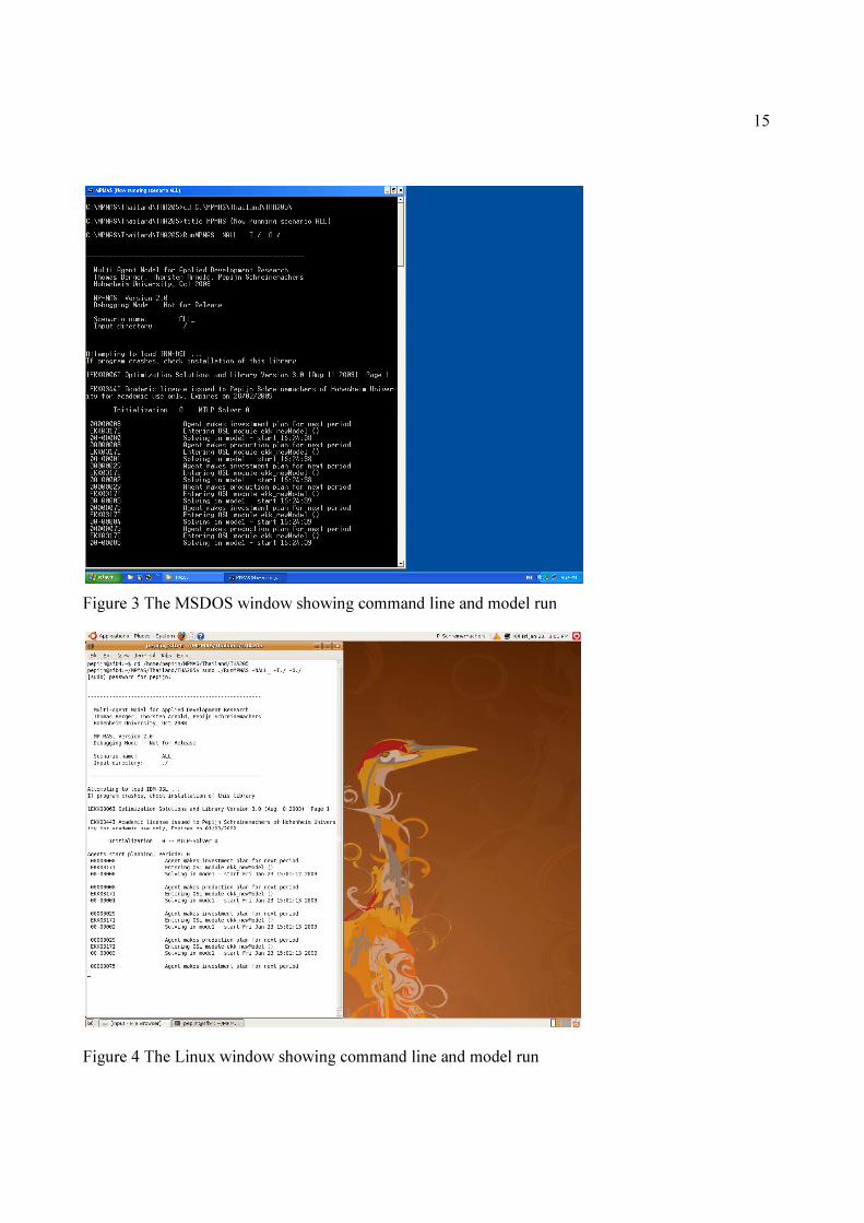
Figure 3 The MSDOS window showing command line and mode

Figure 4 The Linux window showing command line and model run

The MSDOS window showing command line and model run

The Linux window showing command line and model run

15

16

Structure of the model

MPMAS works with a set of input files that are read and processed. It is hence different from

many software applications in that the input data are not entered through specially designed

graphical user interfaces but the user is more or less free to organize the own data.

Input files are written in Microsoft Excel workbooks and contain one or more worksheets with

data and sheets for calculations and notes. The use of Excel workbooks has the advantage that

most users are familiar with it. It is furthermore convenient as workbooks are easily linked and

can contain separate sheets for calculations and documentation of the model. Comments,

explanations, and whole calculations can thus be kept together with the final input data which

greatly simplifies its use. The disadvantage is that `small changes can have big consequences’;

that is, accidentally entering a value in the wrong place can make the program crash.

The general design of input files needs to follow some conventions that are explained in the

following.

WORKSHEET NAMES: The name of each ASCII input file is derived from a prefix specified

in ScenarioManager.xls and the name of the Excel worksheet. For example, if the prefix is set to

“A” and the worksheet is named “MILP” then the input file will be called “A_MILP”. The

worksheet names can therefore not be changed.

ORDER OF THE WORKSHEETS: Excel file contain multiple worksheets. The number of

worksheets converted to ASCII is set in the upper table in ScenarioManager.xls. If, say, two

worksheets are to be converted then the workbook is opened and the first two sheets are taken.

Worksheets with input data should therefore come first in the workbook while worksheets with

calculations and notes should come at the end.

RED-COLORED CELLS: Excel input files need to be well documented by including sufficient

explanation in the worksheets. When converting the Excel worksheets into ASCII these

explanations need to be cleared. Red-colored cells in row 1 indicate that the column should be

cleared while red-colored cells in column A indicate that the row should be cleared.

TEXT COLORS: Different text colors are used to make clear how the cell is calculated.

• Blue numbers contain a formula and refer to cells in the same workbook

17

• Red numbers contain a formula and refer to cells in other workbooks

• Pink numbers are changed by ScenarioManager.xls when converting files to ASCII

• Black numbers are normal cells without formulas

CELL NAMES: One of the advantages of using MS Excel is that workbooks can be linked. If

workbooks are linked then a change of a cell value in one workbook automatically changes this

same value in all other workbooks that are linked to this cell. However, using references such as

“=BasicData!$B$2” has the weakness that if inserting new columns or rows then this reference

is not updated in workbooks that are not currently open. This can be overcome by using textual

cell names instead, e.g. give the cell $B$2 the name “Growth” using the Name Box feature of

Excel.

The fourteen files in the default data set, listed in Table 2, include ScenarioManager.xls and 13

input files. ScenarioManager.xls is used to set up scenarios and to convert the input files to

ASCII format. Each input file contains data for a specific component of the model with the

exception of BasicData.xls which contains parameters used by multiple components. The

number of input files can vary between applications as some components are optional.

The second file is the mathematical programming (MP) matrix (Matrix.xls), which simulates the

decision-making of all agents. This file is central to MPMAS. The function of all other input

files is to calculate parameters in this MP matrix. The remaining input files can be divided into

three groups:

• First, input files that create the population of agents, including their resource endowments

(Population.xls), their spatial attributes (Maps.xls), and their knowledge of and access to

innovations (Network.xls).

• Second, input files containing parameters which are constant over the simulation run,

including general parameters (BasicData.xls), crop water requirements (CropWat.xls), and

the distribution of water rights over agents (WaterRights.xls).

• Third, input files that simulate dynamics over time: demographic changes in agents’

household size and composition (Demography.xls), growth of trees and changes in input

requirements (Perennials.xls), growth of animals and changes in yields and input

requirements over time (Livestock.xls), changes in market prices (Market.xls), changes in

the fertility of soils (Soils.xls), and finally, changes in the water supply (Routing.xls).

18

The general design of input files needs to follow some conventions that are explained in the

following.

Table 2 Overview of the MPMAS input files

Input file Optional Contents

ScenarioManager No To create input files and to manage simulation experiments

Matrix No A generic MP tableau (Mixed Integer Linear Program or

MILP) that simulates the decision-making of agents.

Population No Generates agent populations (household members of various

ages, farm assets, liquidity, and other agent characteristics)

Initial

conditions

Map No All spatial information including the boundary of the

watershed, location of agents and agricultural plots.

Network No Defines networks of innovation diffusion and determines for

each network the level of diffusion at the start of the

simulation.

BasicData No Basic parameter values used in several components of the

model.

Constant

parameters

CropWat Yes Monthly crop water requirement for each crop activity

included in the MP tableau and the efficiency of various

irrigation methods.

WaterRights Yes Defines the distribution of water between agents (water

rights).

Routing Yes The amount of irrigation water and precipitation for each

month and for each year in the simulation run.

Model

dynamics

Perennials Yes Annual yields, variable inputs, and capital needs of perennial

crops.

Livestock Yes Annual yields, variable inputs, and capital needs of farm

animals.

Soils Yes Soil fertility dynamics and crop yield response to soil

nutrients.

Market No All price information in the objective function of the MP

tableau: prices for buying agricultural inputs, farm gate

selling prices, and the off-farm labor wage rate.

Demography No The labor supply for each age of an agent household member

and defines population dynamics such a the probability of

dying and the probability of giving birth.

19

MPMAS input files

ScenarioManager.xls: Managing input files and scenarios

Figure 5 shows a screenshot of ScenarioManager.xls. The workbook is used to change

parameter values in the Excel input files and to convert them to ASCII. The top-left block

specifies the name of the Excel input files; it has an option to include/exclude certain Excel

workbooks, and it specifies for each workbook the number of worksheets to be converted to

ASCII.

Figure 5 Screenshot of ScenarioManager.xls

20

As its name suggests, ScenarioManager.xls, can be used to set up and run different scenarios.

This is done in the lower table. Five scenarios are included in the Default data set but this can be

expanded without change the VBA code. Scenarios are created by adding and/or changing

parameters in this lower table. These parameters are only changed in the ASCII input files while

the Excel input files remain unaffected. The VBA code loops through the workbooks in the

upper table and for each workbook loops through the cell names in the lower table to find a

matching cell name with a parameter to change. For instance, in row 3, a parameter is included

for changing the number of simulation periods in Market.xls to 10 in the first scenario. When

opening Market.xls, the VBA code searches for a cell name “SimYears” and changes its value

to 10. An error message will appear on the screen if the cell name “SimYears” does not exist in

Market.xls. Different scenarios can be set up by adding rows to the table and defining cell

names and parameter values.

Matrix.xls: Agent decision-making

Matrix.xls contains the mathematical programming (MP) tableau, which is a mixed integer

linear programming model (MILP). It optimizes the expected net household income, including

the expected income from farm, non-farm, and off-farm labor and includes current as well as

future expected income streams. A generic MP tableau is defined that can capture the activities

and constraints of every agent. The MPMAS then changes the resource endowments (right-

hand-side values) and switches on and off activities and constraints, to tailor each MP to a

particular agent. Although all MPs are agent-specific, there is therefore no need to define each

MP individually; the software handles this using data from all other files. For instance, prices

are derived from Market.xls, initial resource endowments (right-hand-side values) come from

Population.xls, input-output data for livestock and perennials come from Livestock.xls and

Perennials.xls, while access to innovations comes from Network.xls. All input files contain

information about where in the MP tableau values need to be calculated. The exact location in

the matrix is specified using activity and constraint indices.

Matrix.xls includes twelve categories of data, numbered in column A and listed in Table 3

below.

21

Table 3 Data categories in the Matrix-file

Nr. Name Brief description

1 Parameters and coefficients

Information about the MP tableau, such as the number of activities and constraints and the location of certain activities.

2 Objective function coefficients

The price vector of the MP tableau. The VBA code generates this vector from the MP tableau.

3 Programming matrix The specification of activities and constraints. No missing values are allowed, zeros need to be entered explicitly.

4 Fixed/independent constraints

Fixed/independent constraints can be included, for instance if a right-hand-side value should always take a value 10.

5 Binary for disinvestments

These coefficients specifically relate to the three-step-consumption model (see Market.xls) and should be left blank if this model is not used.

6 Fixing of columns in "consumption mode"

These coefficients also relate to a three-step-consumption model (see Market.xls) and should be set to zero if this model is not used.

7 Fine tuning parameters

Can be used to alter crop yield expectations when taking production decisions to capture risk.

8 Type and range of constraints

Relates to the sign of the constraints (see text)

9 Marked integers Indicates which activities are integers

10 Lower bounds on columns

The minimum value to which an activity can be selected

11 Upper bounds on columns

The maximum value to which an activity can be selected

12 Integers sets / SOS Special integer treatment to speed up solution in the case that the MILP includes many integers.

Structure of the programming matrix

Activities and constraints are identified using an activity and constraint index that starts with

zero (index = 0,1,2, …n). The index of the first activity has the cell name iact_0 while the index

of the first constraint has the cell name icon_0. When inserting or deleting activities and

constraints, it is important that the indices are updated. The VBA will otherwise give a warning

message when converting the workbook to ASCII.

22

The programming matrix needs to be structured in a pre-determined order of activities and

constraints.

Figure 6 shows this structure schematically.

Table 4 shows the correct order of the activities. The first and the last activity are not used and

should be filled with zero values; they contain cell names which position should not be changed

when inserting columns. All selling and buying activities follow next. It is important that these

activities have the same order as in the market file where their prices are listed for each

simulation period. Hiring in labor should come before hiring out labor. Activities that have a

price coefficient come first, followed by all other activities. These can be ordered using any

logic. Lastly come activities called “future selling activities” that refer to the future yield of

investments such as fruit orchards and livestock; these have an entry in the objective function

but have no entry in the current disposable income inside the MP tableau.

Figure 6 Schematic overview of activities and constraints in Matrix.xls

Table 5 shows the correct order of the constraints in the programming matrix. As with the

activities, the first and the last constraints are left blank, i.e., filled with zeros, as these have cell

names that should not be changed. This is followed by a set of constraints that determine the

resource endowments of the agent. This includes liquid means, which is the amount of

accumulated savings by the agent, which is available for investment, variable inputs, or market

Empty

Selling of

crops and

livestock

Buying

inputs

Credits &

deposits

Acess to

innovations Livestock

Growing

crops

Selling

future

products Empty

Empty

Cash

Labor use

Land

Livestock

Perennials

Innovations

Credit

Crop yield balances

Empty

Activities

Constraints

23

consumption. It furthermore includes the available amount of labor, land, livestock, and areas of

plantations, each of which can be subdivided into many categories (e.g., labor into different age

groups, land into soil fertility classes).

Table 4 Order of activities in the programming matrix

Activities Explanation

A. First activity empty, filled with zeros

B. Selling and buying activities All these activities have objective function coefficients (prices) and

have to appear in exactly the same order as in the first block of

entries in the market file. Short-term deposits

Hiring in labor

Hiring out labor

C. All other activities The order does not matter

D. Future revenues from investments Activities with objective function coefficients for selling of future

products, related to investments

E. Last activity empty, filled with zeros

Table 5 Order of constraints in the programming matrix

Activities Explanation

A. First constraint empty, filled with zeros

B. Liquid means This is a transfer row

Labor Labor endowments (can be age and sex-specific)

Land Land endowments (can sub-divided into soil classes)

Irrigation Amounts of available irrigation

Livestock Livestock endowments in heads

Perennial crops Hectares of existing plantations

C. Access to innovations Controlled by the Network.xls, a value is entered if an agent has

access to an innovation otherwise

D. Capital use in period 0 Required cash in period 0 of investment (start-up cost)

Capital use in average year Average amount of capital required

Short-term credit The amount of short-term credit required for an activity

E. All other constraints The order doesn’t matter here

E. Last constraint empty, filled with zeros

24

Information about the activities

Figure 7 shows the upper left corner of the first block of the programming matrix. Activities are

ordered in rows, while constraints are ordered in columns. For each activity, 10 types of

information need to be specified (ordered a-j). The first five of these, are only to assist the

model builder as these are not read by the MPMAS:

THE ACTIVITY INDEX: explained above, starting with number 0.

THE NAME OF THE ACTIVITY: should ideally be short and clear.

THE UNIT OF THE ACTIVITY: e.g., hectare, kilogram, $, etc..

THE SOLUTION VECTOR: or decision variable, shows the optimum solution.

THE OBJECTIVE FUNCTION: which is only required when using the stand-alone-solver.

When using the MPMAS, than it should contain as prices are derived from the market file. The

product of the objective function and solution vector is what is optimized.

The following five variables are required by the MPMAS:

MARKET INTEGERS: set to 1 if the activity can only obtain integer values, 0 otherwise.

FIXING IN CONSUMPTION MODE: only applies to the use of a three-stage optimization

procedure of sequential investment, production, and consumption decisions. When set to 1, then

the selected activities in production mode cannot be changed in the consumption mode. This

captures the timely sequence and irreversibility of investment and production decisions. When

using the one or two-stage optimization, than all values should be set to 0.

LOWER BOUNDS ON THE ACTIVITIES: the minimum value of the decision, usually 0.

UPPER BOUNDS ON THE ACTIVITIES: the maximum value of the decision, usually infinite

(10E31)

The variables are specified left of the programming matrix as shown in Figure 7. This is only to

minimize errors. The MPMAS requires these data to be ordered sequentially as listed in Table

3. Manually entering these data in this order would be cumbersome, especially when the

programming matrix is large. This procedure is therefore automated using the VBA. To do this,

25

the VBA needs to know the location where the information has to be copied from and where it

has to be pasted to. This is provided using cell names as listed in Table 6.

Figure 7 The programming matrix

Table 6 Cell names of activity information

Data category

Matrix-file cell names

Copied from Pasted to

e. Objective function coefficients ObjFunctionCopy0 ObjFunctionPaste

f. Activity type ActTypeCopy0 ActTypePaste

g. Marked integers IntegerCopy0 IntegerPaste

h. Fixing in consumption mode FixConsCopy0 FixConsPaste

i. Lower bound ActLBoundCopy0 ActLBoundPaste

j. Upper bound ActUBoundCopy0 ActUBoundPaste

26

Information about the constraints

Figure 7 also shows the constraints ordered in columns. For each constraint, there are seven

types of information added to the matrix:

TYPE OF CONSTRAINT: directly related to the sign of the constraint equation: a value of 1:

“smaller or equal than”; 2 “greater or equal than”; and 3 “is equal to”.

RANGE OF THE CONSTRAINT: also directly related to the sign of the constraint equation: a

value of 1: “-1E+31”; a value of 2: “-1E+31”, and a value of 3: “0”.

THE LEFT-HAND-SIDE: only used for evaluating the programming matrix and does not have

to be filled in.

THE SIGN: smaller or equal than (“≤”), greater or equal than (“≥”), or is equal to (“ =”). Note

the use of one space before the is-equal sign, because Excel would otherwise treat this sign as a

formula. The sign is not directly used by MPMAS, which uses the type of constraint as a

number.

THE RIGHT-HAND-SIDE: which is only used in the stand-alone-solver version. Right-hand-

side values are agent-specific and are constructed from an agent’s resource endowments (land,

labor, knowledge, etc.).

THE UNIT OF THE CONSTRAINT: e.g. kilogram, hectare, etc. This is not obligatory and is

not read by the MPMAS

THE CONSTRAINT INDEX: which is not directly used by the MPMAS, but is however very

important, as other cells are referenced through this index to specific locations in the matrix.

Like in the case of the activities, the MPMAS requires these data in a specific order as listed in

Table 7. This ordering is handled by the VBA and only needs a correct specification of cell

names as shown in Table 7. If using the split and transposed matrix, than the constraint-related

data needs to be read from separate blocks. The cell names need therefore to be given for each

block separately. The cell names in block 1 get the suffix 1, in block 2 the suffix 2, etc.

27

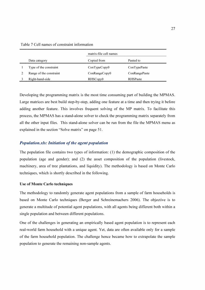
Table 7 Cell names of constraint information

matrix-file cell names

Data category Copied from Pasted to

1 Type of the constraint ConTypeCopy0 ConTypePaste

2 Range of the constraint ConRangeCopy0 ConRangePaste

3 Right-hand-side RHSCopy0 RHSPaste

Developing the programming matrix is the most time consuming part of building the MPMAS.

Large matrices are best build step-by-step, adding one feature at a time and then trying it before

adding another feature. This involves frequent solving of the MP matrix. To facilitate this

process, the MPMAS has a stand-alone solver to check the programming matrix separately from

all the other input files. This stand-alone solver can be run from the file the MPMAS menu as

explained in the section “Solve matrix” on page 51.

Population.xls: Initiation of the agent population

The population file contains two types of information: (1) the demographic composition of the

population (age and gender); and (2) the asset composition of the population (livestock,

machinery, area of tree plantations, and liquidity). The methodology is based on Monte Carlo

techniques, which is shortly described in the following.

Use of Monte Carlo techniques

The methodology to randomly generate agent populations from a sample of farm households is

based on Monte Carlo techniques (Berger and Schreinemachers 2006). The objective is to

generate a multitude of potential agent populations, with all agents being different both within a

single population and between different populations.

One of the challenges in generating an empirically based agent population is to represent each

real-world farm household with a unique agent. Yet, data are often available only for a sample

of the farm household population. The challenge hence became how to extrapolate the sample

population to generate the remaining non-sample agents.

28

The most obvious route would be to multiply

the sample farm households with their

probability weights. Average values in this

agent population would exactly equal those of

the sample survey. Yet, this copy-and-paste

procedure is unsatisfactory for the several

reasons. First, it reduces the variability in the

population. For instance, a sampling fraction

of 20 percent would imply about five identical

agents, or clones, in the agent populations.

This might affect the simulated system dynamics, as these agents are likely to behave

analogously. It becomes difficult then to interpret, for instance, a structural break in simulation

outcomes; e.g., is the structural break endogenous, caused by agents breaking with their path

dependency, or is the break simply a computational artifact resulting from the fact that many

agents are the same? This setback becomes more serious for smaller sampling fractions, because

a higher share of the agents is then identical. Second, the random sample might not well

represent the population. The sample size is small and the sampling error is unknown but can be

large. When using the copy-and-paste procedure, only a single agent population can be created,

while for sensitivity analyses a multitude of potential agent populations would be desired. For

these reasons, the procedure for generating agent populations is automated using random seed

numbers to generate a whole collection of possible agent populations.

Monte Carlo studies are generally used to test the properties of estimates based on small

samples. It is thus well suited for the present purpose as data about a relatively small sample of

farm households is available but the interest goes to the properties of an entire population. The

first stage in a Monte Carlo study is modeling the data generating process, and the second stage

is the creation of artificial sets of data.

The methodology is based on the use of empirical cumulative distribution functions (ECDF).

Figure 8 illustrates such a function for the distribution of goats. The figure shows that 35

percent of the farm households in the sample have no goats; the following 8 percent has one

goat, etc. This function can be used to randomly generate the endowment of goats, and all other

Figure 8 Empirical cumulative distribution

of goats over all households in the sample

29

resources, in an agent population. For this, a random integer between 0 and 100 is drawn for

each agent and the number of goats is then read from the y-axis. Repeating this procedure many

times recreates the depicted empirical distribution function.

Each resource can be allocated using this procedure. Yet, each resource would than be allocated

independently, excluding the event of possible correlations between different resources.

However, actual resource endowments typically correlate, for example, larger households have

more livestock, and more land.

To include these correlations in the agent populations, the sample is divided into a number of

clusters based on statistical analysis (e.g., using cluster analysis). In this example, nine clusters

are formed based on the variable household size, as this variable correlated most strongly with

all other variables. Cumulative distribution functions are then calculated for each cluster of

sample observations. This is illustrated in Figure 9 for the random allocation of goats to the

agents.

Figure 9 Cumulative distribution of goats over households per cluster

30

Implementation in the MPMAS

The ECDFs are included in the file <Population.xls>. This file includes a separate data-sheet for

each cluster (hence nine files in the above example). In each data-sheet two blocks of

information appear. The first block relates to the agents’ household age and sex composition,

while the second block relates to all other assets.

As most resources only come in discrete units (e.g., number of agent household members, heads

of livestock), a piecewise linear segmentation is used to implement the distribution functions.

The default is five linear pieces but more can be specified in the need arises.

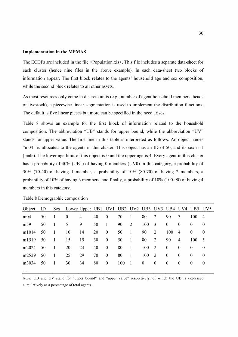
Table 8 shows an example for the first block of information related to the household

composition. The abbreviation “UB” stands for upper bound, while the abbreviation “UV”

stands for upper value. The first line in this table is interpreted as follows. An object names

“m04” is allocated to the agents in this cluster. This object has an ID of 50, and its sex is 1

(male). The lower age limit of this object is 0 and the upper age is 4. Every agent in this cluster

has a probability of 40% (UB1) of having 0 members (UV0) in this category, a probability of

30% (70-40) of having 1 member, a probability of 10% (80-70) of having 2 members, a

probability of 10% of having 3 members, and finally, a probability of 10% (100-90) of having 4

members in this category.

Table 8 Demographic composition

Object ID Sex Lower Upper UB1 UV1 UB2 UV2 UB3 UV3 UB4 UV4 UB5 UV5

m04 50 1 0 4 40 0 70 1 80 2 90 3 100 4

m59 50 1 5 9 50 1 90 2 100 3 0 0 0 0

m1014 50 1 10 14 20 0 50 1 90 2 100 4 0 0

m1519 50 1 15 19 30 0 50 1 80 2 90 4 100 5

m2024 50 1 20 24 40 0 80 1 100 2 0 0 0 0

m2529 50 1 25 29 70 0 80 1 100 2 0 0 0 0

m3034 50 1 30 34 80 0 100 1 0 0 0 0 0 0

…

Note: UB and UV stand for "upper bound" and "upper value" respectively, of which the UB is expressed

cumulatively as a percentage of total agents.

31

The second block of information is the similar, except that these objects have no sex and no

lower and upper age limit, but can optionally have a land requirement (Table 9). The objects

include livestock (e.g., cows and goats), a farm structures (e.g., a henhouse), or hectares of

coffee plantation:

• a female head of the household

• innovation segment: early adopters to laggards

• form of expectations: rational, ..

• liquidity: liquid means available for investments

• leverage:…

The specification of these five assets is not optional. If no data on these are available, then all

values are to be set to zero.

Table 9 Asset composition

Object ID Type LR UB1 UV1 UB2 UV2 UB3 UV3 UB4 UV4 UB5 UV5

Female head 44 -1 0 100 1 0 0 0 0 0 0 0 0

Innovat. 45 -2 0 10 1 40 2 60 3 80 4 100 5

Expect. 46 -3 0 29 0 100 2 0 0 0 0 0 0

Liquidity 47 -4 0 100 500 0 0 0 0 0 0 0 0

Leverage 48 -5 0 89 0 95 0 100 0 0 0 0 0

Cow 2 8 .91 50 0 70 2 80 4 90 7 100 23

Goat 3 8 .13 40 0 60 1 80 3 90 4 100 8

Cow in shed 4 8 0 100 0 0 0 0 0 0 0 0 0

Coffee 1 14 1 1 30 0 40 0 60 0 80 0 100 4

…

Note: LR stands for land requirement; UB and UV stand for "upper bound" and "upper value" respectively, of

which the UB is expressed cumulatively as a percentage of total agents.

32

Maps.xls: The physical landscape

MAS models of land-use/cover change (MAS/LUCC) couple a cellular component that

represents a landscape with an agent-based component that represents human decision-making

(Parker et al 2003). The landscape component is defined in the map-file. It contains six spatial

layers of information as summarized in Table 10. The interface offers two options for analyzing

a matrix file. The first is “Solve again”, which takes the matrix file, removes all string values

from the file, saves it under a different name, and solves the file again using an executable

called “MilpCheck.exe”. Three different solving routines are available and if the matrix is

feasible then the solution vector is saved as a separate file.

The other option “Back to Excel” takes the matrix file and copies and pastes its values (matrix

coefficients, bounds, and right-hand-side values) to Matrix.xls saving it under its original name,

but with the extension “.xls”. If the matrix has first been analyzed using “Solve again” then the

solution vector is automatically imported into the file. This option is suitable for analyzing

matrices that were infeasible.

The information is numerically encoded and organized in a raster format. Grid cells with no

information get a value “-1”. Each cell represents a certain amount of land, e.g., 1 hectare.

The map-files can be produced in two ways: in a Microsoft Excel workbook, if the number of

columns is less than 256 and which is then converted to plain text format using

ScenarioManager.xls, or in ArcView GIS using the exporting routine to save it in ASCII format.

All maps have to be in a grid cell format. Polygons must be converted to grid cells. Yet, by

defining the grid sufficiently small, the grid format can approximate any polygon.

Table 10: Spatial layers in Map.xls

Nr. Layer

1. The location of agents’ farmsteads

2. Each agents’ membership of a population

3. Each agents’ membership to a population cluster

4. Each agents’ membership to an innovation segment

5. The location of agents’ plots

6. The soil type of each plot

33

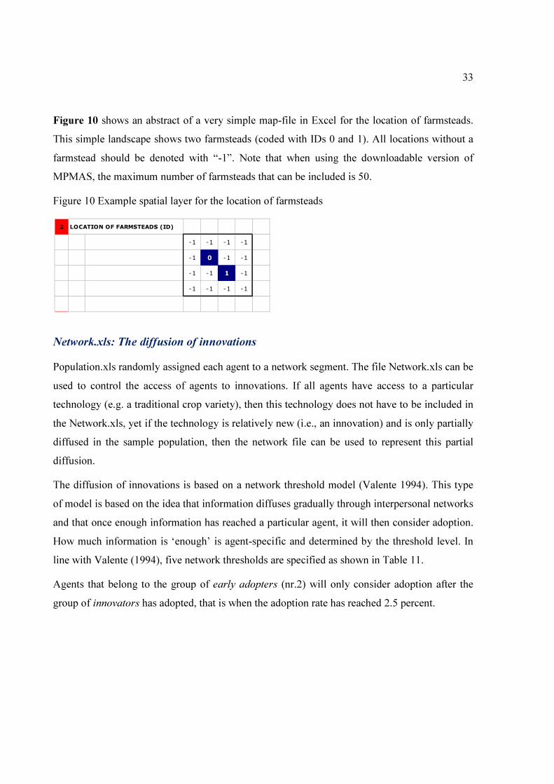
Figure 10 shows an abstract of a very simple map-file in Excel for the location of farmsteads.

This simple landscape shows two farmsteads (coded with IDs 0 and 1). All locations without a

farmstead should be denoted with “-1”. Note that when using the downloadable version of

MPMAS, the maximum number of farmsteads that can be included is 50.

Figure 10 Example spatial layer for the location of farmsteads

Network.xls: The diffusion of innovations

Population.xls randomly assigned each agent to a network segment. The file Network.xls can be

used to control the access of agents to innovations. If all agents have access to a particular

technology (e.g. a traditional crop variety), then this technology does not have to be included in

the Network.xls, yet if the technology is relatively new (i.e., an innovation) and is only partially

diffused in the sample population, then the network file can be used to represent this partial

diffusion.

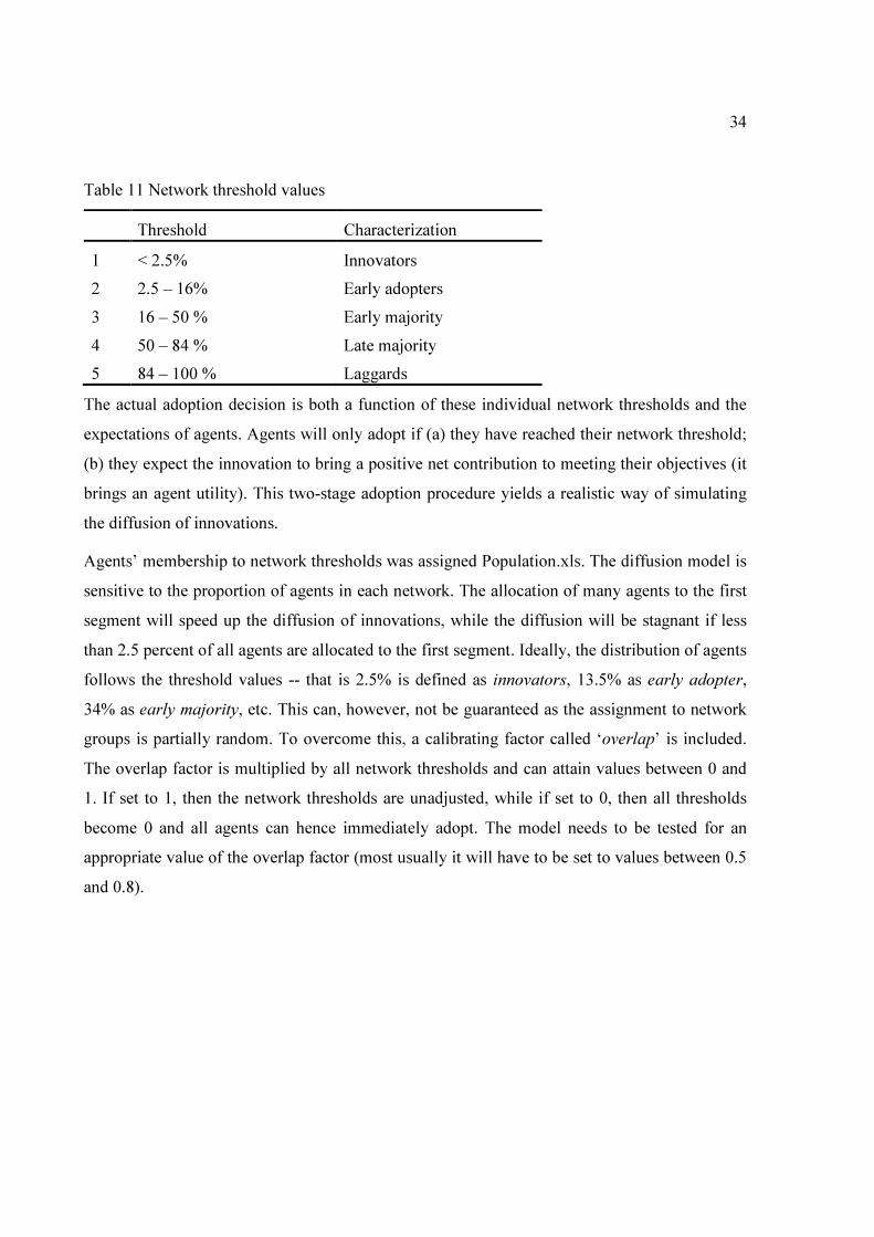
The diffusion of innovations is based on a network threshold model (Valente 1994). This type

of model is based on the idea that information diffuses gradually through interpersonal networks

and that once enough information has reached a particular agent, it will then consider adoption.

How much information is ‘enough’ is agent-specific and determined by the threshold level. In

line with Valente (1994), five network thresholds are specified as shown in Table 11.

Agents that belong to the group of early adopters (nr.2) will only consider adoption after the

group of innovators has adopted, that is when the adoption rate has reached 2.5 percent.

2 LOCATION OF FARMSTEADS (ID)

-1 -1 -1 -1

-1 0 -1 -1

-1 -1 1 -1

-1 -1 -1 -1

34

Table 11 Network threshold values

Threshold Characterization

1 < 2.5% Innovators

2 2.5 – 16% Early adopters

3 16 – 50 % Early majority

4 50 – 84 % Late majority

5 84 – 100 % Laggards

The actual adoption decision is both a function of these individual network thresholds and the

expectations of agents. Agents will only adopt if (a) they have reached their network threshold;

(b) they expect the innovation to bring a positive net contribution to meeting their objectives (it

brings an agent utility). This two-stage adoption procedure yields a realistic way of simulating

the diffusion of innovations.

Agents’ membership to network thresholds was assigned Population.xls. The diffusion model is

sensitive to the proportion of agents in each network. The allocation of many agents to the first

segment will speed up the diffusion of innovations, while the diffusion will be stagnant if less

than 2.5 percent of all agents are allocated to the first segment. Ideally, the distribution of agents

follows the threshold values -- that is 2.5% is defined as innovators, 13.5% as early adopter,

34% as early majority, etc. This can, however, not be guaranteed as the assignment to network

groups is partially random. To overcome this, a calibrating factor called ‘overlap’ is included.

The overlap factor is multiplied by all network thresholds and can attain values between 0 and

1. If set to 1, then the network thresholds are unadjusted, while if set to 0, then all thresholds

become 0 and all agents can hence immediately adopt. The model needs to be tested for an

appropriate value of the overlap factor (most usually it will have to be set to values between 0.5

and 0.8).

35

Table 12 Innovations

Nr. Parameter Explanation

1 Object ID This should match with the object ID in all other files (e.g. <perennials.xls>,

<population.xls>, and <demography.xls>.

2 Type The type of object. There are two basic types: Objects with a negative type refer

to agent characteristics, while objects with a positive type refer to asset

characteristics (incl. innovations).

3 Divisibility Set to 1 for all divisible innovations. E.g., a cow is indivisible (set to 0) while a

hectare of coffee is divisible (set to 1)

4 Acquisition costs The purchasing price of an innovation in the first year. For livestock, make sure

this is consistent with <livestock.xls>.

Note that this cost refers only to “proper investments”, i.e. productive activities

with a gestation between first input use and full output of more than 1 year. If

shorter than 1 year, then the price must be included in file <Market.xls>.

5 Lifetime The maximum age of an object. For example, a coffee plantation lasts 12 years,

and cows are culled before they turn 10 years old.

6 Suitability The soil types an innovation can be used on, if not restricted to any soil type then

set the suitability to 0.

7 Minimum

investment

Optionally a minimum amount can be specified. E.g, when investing into a new

coffee plantation, the investment should be more than 0.2 ha.

8 Column The activity index in the programming matrix. In case of investment objects, the

MATRIX includes two separate activities: one for production and one for

investment. This index must refer to the production activity.

9 Row The constraint index in the programming matrix.

10 Permanent crop

yield

The row coordinate in the programming matrix where the yields appear (-1 if not

a permanent crop)

11 Coefficient The pieces per unit of the investment good (e.g., days/laborer)

The solution in the investment mode is taken and enters the production mode after

multiplication with this factor. The factor is therefore used to convert the units in

the solution vector of the investment mode to units of the RHS in the production

mode.

12 Level of

innovation

Specifies for what segment the innovation is accessible, if accessible for all set to

0.

13 Availability The year at which the innovation is introduced into the population

14 Accessibility The year at which the innovation can be acquired for the particular innovation

segment.

15 Share own capital The share of the acquisition cost that needs to be paid from own liquid means.

16 Interest rate on

borrowed capital

For what is not paid from own means an additional interest cost is incurred.

36

Network.xls lists all innovations and specifies various types of information for each of these as

is briefly explained in Table 12. The network-file uses three types of interest rates. (1) The long-

term interest rate is the interest over borrowed capital with a gestation of longer than one year.

(2) The short-term interest rate is the rate for borrowing capital from, say a bank, for a period of

one year. (3) The interest rate on equity is the rate you receive when depositing money at a bank

(say, at your current account). This is the opportunity costs of capital. In absence of any banks

or informal savings, this rate can be set very low.

BasicData.xls: General parameters

Parameters that do not immediately relate to a single input file but are required by several

separate model components are included in BasicData.xls. About 48 parameters are included in

this file. For instance, the choice of consumption model is included in BasicData.xls because

this impacts both on the matrix-file and on the market-file. The file is organized in eight

categories of parameters as shown in Table 13. Most parameters in this file are self-

explanatory.

Table 13 Parameters in BasicData.xls

Category Explanation

1 General parameters Integers counting the frequency of same events, like the number of catchments,

villages, networks, etc.

2 Innovation parameters Various parameters that allow the user to fine-tune the innovation diffusion

process, such as the ‘overlap’ parameter described in Section 6.

3 Rental markets For making land markets endogenous in the model

4 Policy parameters For the simulation of policy options such as subsidies for permanent crops

5 Switches for various sub-

models

Defines which consumption is implemented and whether there is a crop growth

model, livestock or perennial crop model. If not then no respective file is read

by the program.

6 Soil information Defines the size of a single grid cell in hectares and defines which number of

different soil types and classes. Soil classes refer to land suitability.

7 Debugging of the

programming matrix

The most important dynamics can be switched off using these options: (a) aging

of agent household members and assets; (b) and updating of soil fertility (only if

a soil model is defined). In addition matrices can be saved by entering a matrix

number.

8 Fine-tuning of the solver This tells the solver how long it can maximally take to solve a single MP model

or how many iterations is can go through.

37

CropWat.xls: Crop water requirements

Crop yields were modeled following the FAO CropWat model (Clarke et al. 1998, Smith 1992).

The workbook CropWat.xls specifies for each crop activity that appears in Matrix.xls the crop

water requirement and the crop yield potential. For each selected crop activity in the MP

tableau, MPMAS will recalculate a crop yield based on the crop water requirement and the crop

water supply—the latter specified in Routing.xls and is explained in the next section.

The crop-water requirement (CWR) for crop c in month m is the product of a crop water

coefficient (Kc), the potential evapotranspiration (ET0), and the planted area (Area):

CWRc,m = Kcc,m* ET0m * Areac,m (1)

in which ET0 is a function of the local climatic conditions and can be derived from CropWat

7.0. The Kc values can be obtained from specialized literature or as standard values in the

CropWat model.

Monthly values for CWR do not change over time and are therefore specified in the workbook

CropWat.xls. Each of the crop activities specified in Matrix.xls also needs to be included in

CropWat.xls. In CropWat.xls the activity and constraint indices in the MP tableau are specified

for each crop activity and are linked to Matrix.xls.

The CWR can either be met through irrigation (IRR) or precipitation—converted into effective

precipitation (EP) to capture the share of precipitation that is actually available to the crop,

depending on its growth stage. The calculation of effective precipitation is rather complex in

CropWat and was simplified using a regression equation. The equation can be parameterized by

inserting into CropWat a large range of precipitation values and crop water requirements for a

selection of crops and then obtaining the EP values. The EP values can then be regressed on the

crop water requirements and precipitation using ordinary least squares:

EPcm=a+b1*CWRcm+b2*(CWRcm)2+c1*PRECm+c2*(PRECm)2+d*CWRcm*PRECm (2)

The part of the crop water requirement that is unfulfilled by either precipitation or irrigation is

called the deficit irrigation (DIRR):

DIRRcm = CWRcm – ERcm – IRRc (3)

38

If there is deficit irrigation then the crop yield is reduced. The magnitude of the deficit is

expressed as the quotient of the deficit irrigation and the crop water requirement

(DIRRcm/CWRcm), which is called the Kr value. In reality it matters much in what stage of the

growing period the water deficit occurs. Yet, as a simplification, the quotients of deficit

irrigation and the crop water requirement are simply averaged over all months with non-zero

crop water requirements:

�� = �� ∗ ∑��

��

�� > � (5)

Following Berger (2001) it is assumed that the crop yield is lost completely if the average Kr

falls below 0.5, while for Kr values greater than or equal to 0.5 the average Kr value is

multiplied by the crop yield potential (YPOTc) to simulate the actual crop yield (Yc):

�� = �� ∗ �� ≥ .� �� < .� � (4)

Routing.xls: The crop water supply

Routing.xls simulates the irrigation water supply as based on the Edic-cedec model (Berger

2000). The physical landscape is divided into irrigation sectors while the irrigation water supply

is defined per sector. There are three sources of irrigation water in MPMAS:

• River flows: This is the water supply from streams in the watershed

• Surface runoff from neighboring irrigation sectors: The runoff from neighboring irrigation

sectors.

• Lateral flows: The sub-surface flows from neighboring irrigation sectors.

The first three worksheets in Routing.xls define the quantity of water from each of these

sources. The first worksheet <EdicRiverFlows0> defines this quantity in m3/second while the

two other worksheets <EdicSurfaceRunoff0> and <EdicLateralFlows0> define it as a

proportion of the river flows. These last two sheets contain a matrix in which the surface and

sub-surface flows between all sectors can be defined. If irrigation water is only directly derived

from streams then all values can be set to zero.

39

The last worksheet in Routing.xls, <EdicIrrigationMethods0>, defines the efficiency of various

irrigation methods and contains parameters of the Edic-cedec model.

Table 14 Efficiency of various irrigation methods defined in Routing.xls

Name Surface runoffs at

night

Evapotranspiration

surface subsurface groundwater

Flood 0.111 0.267 0.400 0.133 0.089

Furrow 0.111 0.400 0.311 0.111 0.067

Terracing 0.111 0.544 0.233 0.067 0.044

Drip 0.111 0.800 0.000 0.053 0.036

Improved Furrow 0.111 0.444 0.267 0.111 0.067

Advanced Furrow 0.111 0.444 0.267 0.111 0.067

Sprinkler 0.111 0.711 0.067 0.067 0.044

Tape 0.111 0.800 0.000 0.053 0.036

Center Pivot 0.111 0.800 0.000 0.053 0.036

Micro sprinkler 0.111 0.800 0.000 0.053 0.036

Region.xls: The distribution of water over agents

Region.xls defines the distribution of water rights over agents. Water rights are defined as a

proportion of the total irrigation water supply of an irrigation sector that an agent is allowed to

use. This proportion is assumed constant over the whole year and during all years in the

simulation run.

MPMAS has two options for distributing water over agents:

1. Random water rights: Similar to the data structure in Population.xls, the water rights can

be distributed over agents randomly. Upper and lower bounds can be defined for each

inflow and for each sector.

2. Actual water rights: For each agent it is defined what proportion of the total irrigation

water supply per sector and per inflow the agent can use.

40

Perennials.xls: Parameters of perennial crops

Whereas the population file specifies the course of human life, the permanent crop file specifies

that of trees. It contains the following information for each year in the life span of a permanent

crop:

• yield

• pre-harvest costs (e.g., spraying)

• harvest cost

• total labor requirement

• total machinery requirement

• peak labor requirements

Furthermore, it specifies the acquisition cost and life span, both of which should be the same as

specified in the network file.

Because alternative levels of input use are possible for a crop, a separate permanent crop

activity is specified for each input level. For instance, in the Uganda case, coffee can be grown

on five different soil types, with 3 alternative levels of labor use, and with or without fertilizer;

this translates into 30 different coffee activities. Switching between input levels and between

soil types is thereby prevented and to switch input levels the agent is required to fulfill the

acquisition cost and start anew in year 0.

Livestock.xls: Parameters of livestock

The livestock file is similar to the permanent crop file in that different parameter values can be

specified for each year. The livestock file is, however, different from the permanent crop file in

that more than one output can be specified and the matrix coefficients of these outputs are

directly entered in this file, rather than the network file.

The first two outputs of each livestock type are gain in live weight, which is specified

cumulatively, and numbers of female offspring. Female offspring is treated differently as this

has a course of life of its own starting with year zero. Male offspring remains in the file as its

sole purpose is meat production.

41

Livestock.xls is furthermore different from the permanent crop file in that it allows labor to be

specified per period, while in the permanent crop file only average labor is specified which is

distributed over all periods according to fixed coefficients in the programming matrix.

Soils.xls: Soil fertility dynamics and crop yields

Soils.xls contains parameter values for a biophysical model to simulate soil fertility changes and

the resulting crop yields as based on the Tropical Soil Fertility Calculator (TSPC). This

integrated model was developed for an MPMAS application to Uganda. For more details about

this component the reader is referred to Schreinemachers et al. (2007) and Schreinemachers

(2006). The TSPC does not have to be included in the model but can be switched off in

ScenarioManager.xls. If switched off then the file soils.xls does not have to be included in the

input data.

Market.xls: Market prices and consumption

Market.xls contains two types of information. First, it specifies market prices for all products

and second, it specifies which type of consumption model is implemented. Each is described in

the following.

Market prices

Market prices define the prices for all tradable goods and is equivalent to the objective function

of the MP model. Market prices include: (1) selling prices of agricultural products; (2) buying

prices of food products; (3) buying prices of seed, chicks and fertilizer; and (4) prices of leasing

in a tractor, and hiring in or out labor. The MPMAS software copies these values and pastes

them into the MP matrix. The order of these goods must therefore be the same as in the file

<matrix.xls>.

All market prices are exogenous in the model and need to be defined for each period in the

market-file. The effect of price changes can be simulated by adjusting the prices in this file; this

file can therefore be used to test various price-related scenarios.

42

Market prices include the price of hiring labor in and hiring labor out. Make sure that the price

of hiring in is greater than the price of hiring out otherwise the MP model might become

unconstrained. A higher price for hiring in is justified by transaction and monitoring costs.

A special type of prices are ‘future prices’, these are expected selling prices related to

investment activities such as livestock or trees. These, for instance, include milk and meat.

These products cannot be sold in the same year of investment and hence do not add to the

current revenues but only to the future income. Whereas the current prices always enter the

matrix in a pre-determined order as the first activities, the user can determine where the future

prices enter the matrix by specifying an activity index for each entry. Hence, the order in which

they appear in the matrix file does not matter. Activity indices are ideally linked to the matrix-

file so that they are automatically updated when adding activities or constraints to the matrix.

Two types of consumption models can currently be specified: one very basic and one very

complicated model. More intermediate consumption models will be included in the future. The

choice of consumption model should be included in BasicData.xls. If using the extended

consumption model then Matrix.xls needs to include the consumption model in the matrix.

The basic consumption model

When using the basic consumption model, then consumption is handled by simple heuristics

outside the MP model and after the income level has been determined. Buying activities for

food products do therefore not have to be specified in the market file. The basic consumption

model simply specifies how much of the income will be consumed. The remainder will be

added to the agent’s cash endowment and is available for investment in the next period. The

basic model requires specification of three parameters:

1. Extra consumption [proportion]: This is the proportion of each additional monetary unit that

is consumed and ranges between zero and one. If set to zero then no income is consumed

and all is saved; if set to one then all income is consumed and nothing is saved.

2. Minimum consumption per head/year [monetary value]: This value specifies the minimum

amount of income that is consumed by each member of an agent’s household. It must be set

to a positive value.

43

3. Foregone consumption [monetary value]: In case that income is too low to meet the

consumption specified by (1) and (2) then this value determines the proportion by which the

consumption level is to be reduced. If set to zero then the minimum consumption level is

reduced to zero. If set to one then the consumption is not adjusted downward.

The extended consumption model

If using the extended consumption model then the program uses a three-stage solving procedure

of investment, production, and consumption (the last stage is not needed if using the basic

consumption model). The assumption is that production and consumption decisions are

inseparable because of market imperfections as is typically the case in rural areas of low-income

countries (Sadoulet and de Janvry, 1995). Different from the basic consumption model, that

simply allocates part of the revenues to consumption and the rest to savings, the extended model

implements the consumption decision within the MP model so that production and consumption

decisions are simulated simultaneously. Because the parameters of the extended consumption

model are household-specific its implementation requires much additional input in both the

market- and the matrix-file.

The implemented consumption model itself has a three-step procedure of savings, food/non-

food expenditures, and expenditures on specific categories of food products. The model is

described in Schreinemachers (2006) and Schreinemachers and Berger (2006b). Including this

model requires the estimation of econometric models at each step. The advantage of this model

is that it allows a detailed simulation of food security dynamics. If food security is not much of

an issue and market imperfections are few then the basic consumption model is preferred.

Savings

In the first step of the system, agents decide how much of their income to expend and how

much to save. Let the variable SAV be the savings and INC the disposable income, H the

household size measured in an equivalence scale (joules), D the matrix of district dummies, and

α0 a constant term. The amount of savings is specified as a quadratic function of disposable

income:

44

∑−

=

++++=

1n

1i

i4,3

2

210DαHαINCαINCααSAV 0αwith

2> (5)

in which the alfas are the parameters to be estimated. Micro-economic theory suggests that the

share of savings increases with income, which is the case if α2 is positive.

Food/non-food expenditures

Total expenditure (TEX) is the income available to spend, which is derived from the income

identity:

TEXSAVINC += (6)

In the second step, agents decide how much of this total expenditure to allocate to food (FEX)

and non-food items (NEX). A modified version of the Working-Leser model quantifies this

relationship (Hazell and Roell 1983):

DβHβTEXlnββv40

1n

3210 ∑=

+++= (7)

in which v is the expenditure share on food and the betas are parameters to be estimated. It

follows that the value of food expenditures (FEX) equals TEX*v/100 while NEX can be derived

from the parameter estimates using the properties of symmetry and adding up.

Expenditures of food categories.

In the final step agents decide to spend their food budget on broad categories of food products.

The use of categories instead of individual items gives agents more scope for substitution. The

third step is quantified using a linear approximation of the Almost Ideal Demand System

(LA/AIDS) (Deaton and Muellbauer 1980):

DδHδ)ln(M/Pδplnδδw40

1n

k4,k3,

k

*

k2,llk,1,k0,k ∑∑=

++++= (8)

45

where the subscripts k and l denote individual food categories of a total of n categories

(k,l=1,2,..,n) and the gammas denote parameters to be estimated. The variable wk is the share of

category k in the total food budget; M is per capita food expenditures measured in an

equivalence scale for household size. P* is an index of prices, which in the original (non-linear)

version has a translog functional form but in its linear version can be replaced by the logarithm

of the Stone geometric price index (Deaton and Muellbauer 1980):

∑=k

kk

* plnwPln (9)

Demography.xls: Population dynamics and labor supply

The age of each household member naturally changes over time. Aging impacts on the

household labor supply and is therefore an important dynamic in the model. Demography.xls

specifies age-specific variables that optionally include, apart from labor supply, mortality,

fertility, and nutritional requirements. Table 15 shows an abstract of this file, for the labor

category of unskilled male labor for the first 4 years.

Labor supply can be estimated from farm household survey data. If the programming matrix

uses an agricultural production function that relates output to labor use, then it is important that

the labor supply is estimated from the same data source. Data on time allocation are typically

inaccurate and variable between surveys. The importance here is not so much to get an accurate

estimate but an estimate that is consistent with the production function used.

Mortality and fertility are specified in terms of the probabilities of dying and giving birth.

Mortality and fertility can be obtained from official statistical sources or demographic studies.

Make sure that the probability of dying at the maximum age is set to unity otherwise the

program might crash.

46

Table 15 Abstract of the demography file

Food nutrition, such as calories and protein, can be included to quantify food security. This is

only useful in case a detailed food consumption model is included that estimates food

consumption into detail. This consumption model, simulating the nutrient supply, would have to

be specified in Market.xls; while Demography.xls estimates the nutritional demand and the

balance of the two would be an indicator of food security. Food nutrition is location specific and

moreover depends on the intensity of physical activity performed. One possible source of

country-specific default values is James & Schofield (1990).

Additional features

MPMAS includes additional features that assist the model builder in tracing back changes,

analyzing certain MP models, looking at the results, or solving the model in a stand-alone

version. Each of these options is detailed in the following.

XChanges.txt

This is a plain text file in which the model builder can keep a diary of changes made to the

model. We previously recommend that the modeler proceeds in a step-wise fashion in which

small changes are made one by one after which the model is solved, the complete file set is

saved, and a copy is used as a basis to make a subsequent change. In this way, the modeler

always has one running version of the model and if the MPMAS reports an error than one can

always go back to this latest running version and try to make the change again, but perhaps in

B. Unskilled male members

Career ID 64

Number of different ages (lifespan) 100

Age 0 Age 1 Age 2 Age 3

Sex-age group 1 1 1 1

Labor hours / year 0.0000 0.0000 0.0000 0.0000

Mortality (probability of dying) 0.0764 0.0257 0.0123 0.0074

Fertility (probability of giving birth) 0.0000 0.0000 0.0000 0.0000

Energy needs (billion joules/year) 1.0684 1.5055 1.7312 1.8747

Protein needs (kg/year) 5.1100 8.0300 8.0300 9.4900

47

smaller steps. If all changes are well documented in the file <XChanges.txt> then it will be

easier to detect the source of possible errors when these are encountered.

Check matrix files

If an MP model for a particular agent is infeasible then MPMAS saves it with the extension

“.mip” in the folder out/test. The name syntax of saved programming matrices is shown in

Figure 11. In ScenarioManger.xls users can also request MPMAS to save additional matrices,

either by either:

• Specifying the matrix (as a positive number) in the option “Save a matrix […]”

• Specifying the agent ID (as a negative number) in the option “Save a matrix […]”

• Including the flag “-M” in the MPMAS command line will save all matrices

Figure 11 Name syntax of saved MP matrices

The agentID is an integer value that identifies each agent. Note that the numbering does not

start at 0 but at 1. AgentID 0 is reserved for a ‘special agent’: it contains all land that is not

currently allocated to all other agents. This agent does not solve any MP model; it just acts as

storage for the village (or subcatchment). Hence, for each village (or subcatchment) the

remaining land is stored in a separate agent. Because of this procedure the agentID from the

map-file might be different from the agentID used internally by the program, which is only in

the case of multiple villages/subcatchments. It is therefore recommended to adjust the agentID

in the map-file by not assigning the first ID to an agent (for each village/subcatchment).

period number of matrix loaded

0_0_1MILP0.mip

SubcatchmentID agentID

48

If a matrix is infeasible then this can indicate one of the following:

(a) there is a problem with some of the input files that update the matrix;

(b) there is a problem in the design of the matrix; or

(c) there is a problem in the source code of the MPMAS.

Most frequently the first or the second option will be the case as the model has been tested

extensively. The produced error matrix has a format similar to the matrix input file in ASCII

format (MILP.dat), except that it has textual remarks for each block of information. It will be

difficult to study the matrix in this format, for which reason the macro “Check matrix files” was

developed. It is accessed through the MPMAS menu bar in ScenarioManager.xls or by using the

shortcut ALT+CTRL+M. It opens a Graphical User Interface that suggests which matrix files

are available from the last model run (Figure 12). The interface offers two options for analyzing

a matrix file. The first is “Solve again”, which takes the matrix file, removes all string values

from the file, saves it under a different name, and solves the file again using an executable

called “MilpCheck.exe”. Three different solving routines are available and if the matrix is

feasible then the solution vector is saved as a separate file.

The other option “Back to Excel” takes the matrix file and copies and pastes its values (matrix

coefficients, bounds, and right-hand-side values) to Matrix.xls saving it under its original name,

but with the extension “.xls”. If the matrix has first been analyzed using “Solve again” then the

solution vector is automatically imported into the file. This option is suitable for analyzing

matrices that were infeasible.

49

Figure 12 Screenshot of “Check matrix files”

A few tips for finding an error in a programming matrix

To find an error and what causes it can sometimes be a challenge. Here are some tips that could

help:

Find out whether the matrix is an investment model or a production model. The investment

model has a value ‘1’ in the right-hand-side of the first activity (called the investment switch),

which allows investments in perennial crops. If no value ‘1’ appears then the matrix is a

production model.

• Check whether all right-hand-side values have positive values

• Check for strange combinations of right-hand-side values:

50

• Is male or female adult labor zero or very high?

• Is land zero or very high?

• Are livestock numbers very high?

• After finding a ‘suspicious’ value in the programming matrix then change it and try to

solve again.

In addition, the IBM Solver can help to locate an error in the matrix. Often it is able to point to a

specific cell value (by row and constraint index) that makes the problem infeasible. For this, the

error matrix can be solved using the stand-alone-solver, which is the file MilpCheck.exe..

XResults.xls

Model results can be analyzed using standard statistical packages such as STATA, SPSS, or

MATLAB. The file XResults.xls was developed for the default data set to get a quick look

into the results of the model. Figure 13 shows the interface of this file. The file contains VBA

code that imports two types of output files:

u-files: these contain the price and solution vector; and

k-files: these contain the right-hand-side values and left-hand-side values.

All output files are described in a following section of the manual. In addition to the VBA

importing routine, the file does some simple analyses of a few selected variables using database

functions in Excel. Users can add other types of analyses.

51

Figure 13 XResults.xls

Solve matrix

The MP tableau in Matrix.xls can be solved independently. For small tableaus, the standard

solver available in MS Excel can be used yet for larger tableaus the OSL can be used as a stand-

alone solver as shown in Figure 14. This macro will save Matrix.xls and convert it to ASCII,

creates a batch file calling the IBM-OSL, re-open Matrix.xls and import the solution vector into

the matrix. We note that the macro only works with Matrix.xls.

52

Figure 14Solving Matrix.xls with the stand-alone solver

XSingleAgents.xls

The developed programming matrix (Matrix.xls) can be tested for different sets of right-hand-

side values using the file XSolver.xls. Figure 15 shows the main interface of this file. The VBA

code is run through the MPMAS menu bar in Microsoft Excel. The VBA code goes through the

following procedure: Right-hand-side values from the worksheet <RHS> are copied to the

matrix (Matrix.xls) and saved it in mtx-format. Make sure that the right-hand-side value has the

same range otherwise an error message will pop up to the screen.

A batch file calling MilpCheck.exe is created for and run. This will create an MS-DOS pop up

window for each file that is solved. Each feasible matrix will result in a solution vector saved to

53

the hard disk; these files are recognizable by their extension “.pri” (standing for primal). All

solution vectors are imported to the worksheet <Analyze>. The results are shows in simple

charts, which can be adjusted or extended by the user.

Figure 15 XSolver.xls

54

Scenario output files

Scenario results are written to the folder /out. A first set of output files returns the outcomes

of the random agent generator (Table 16). The first contains the input as read by the program

and the second contains the output representing the generated agent population. This second

file, with extension .LT2, can be analyzed and compared with the survey data. For each period

in the simulation, there is a set of output files in plain text (ASCII). There are nine types of files

listed and shortly described in Table 17.

.

Table 16 Agent generation output files

Nr. Extension Description

1 .LT1 Input to the random agent generation. This contains the asset assignment as in

the file <Population.xls> with a separate file for each cluster.

2 .LT2 Output from the random agent generation. Assigned assets to each agent with a

separate file for each cluster of agents. Note that the first agent is the ‘special’

agent which comprises all non-allocated land.

Table 17 Output files

Nr. suffix Description

1 _at Agent exit data (e.g., due to bankruptcy or out-migration)

2 _dt The diffusion of innovations

3 _kt Available and used resources

With _xkt for agents having exited the population

4 _pt Agent performance (e.g. income, depreciation, liquidity, etc.)

With _xpt for agents having exited the population

5 _ut The solution vector (primal)

With _xut for agents having exited the population

6 _yt Crop yield information (only when having yields endogenous in the model)

7 _w Sector water data

8 _l Land data

9 diff Innovation diffusion over all periods in one file

55

Each row in the p, u, and k-files contains information on a separate agent. The first 13 columns

are the same in each of these three files and listed in Table 18.

Table 18 First entries in the k, u & p-files

Nr. Short name Explanation

1 typ_str Type of information:

1: performance data (p-file);

2: primal solution (u-file);

3: objective values (u-file)

4: available capacity (resources) (k-file)

5: actually used capacity (k-file)

2 aID Identifies the agent

3 catchID Identifies the (sub-)catchment or village

4 secID Identifies the agent sector

5 fstID Identifies the farmstead as read from the file <map.xls>

6 popID ID of agent population

7 clustID Identifies the population cluster (i.e., each sheet in the file <population.xls> is

a separate segment

8 nwID Identifies the network through which innovations diffuse (e.g., separate

networks of large-scale commercial and family farms)

9 segID Identifies the innovation segment (0,1,2,3,4)

10 expectID Type of (price and yield) expectations

11 colorID Color of grid cell in the map

12 xcoord x-coordinate of the farmstead (column number in raster map)

13 ycoord y-coordinate of the farmstead (row number in raster map)

56

Table 19 Entries in the a-file: agent population dynamics


1 GiveUp Type of information:

14=planning error

15=reason of exit

2 nwID Number of separate networks

3 segID Segment ID

4 f_per_seg Number of agents remaining in each segment

5 nr_m_plan Number of planning mistakes

6 nr_giveup_vol Number of agents that give up voluntarily (e.g., migrate out due to high

opportunity costs outside farming)

7 nr_giveup_invol Number of agents that were forced to give up (e.g., bankruptcy)

The a-file contains information on the agent population dynamics, such as exits due to

migration and bankruptcy. Table 20 shows the structure of this file.

Table 20 Entries in the d-file: Innovation diffusion

First column ID Explanation

06 Number of users of an innovation (absolute value)

07 The total acreage of all users of an innovation (absolute value)

08 Total Gross Margins (absolute value)

09 Value Added (absolute value)

10 users (percentage)

11 acreages of users (percentage)

12 Total Gross Margins (percentage)

13 Value Added (percentage)

57

Table 21 Exit of agents

Code Explanation

-1 Bankruptcy / forced migration: The liquid means are less than zero.

-2 Voluntary migration: The opportunity cost of labor (defined in Network.xls) is greater than

the returns from the farm times the migration full factor (also defined in Network.xls)

-3 No household members left: Because of mortality and fertility rates (defined in

Demography.xls) the agent has lost all household members and thereby seizes to exist.

-4 No active labor force: The labor supply is zero (the labor supply for each age and sex

category is defined in Demography.xls).

-5 No adult labor force: The agent household has only children. Note that the difference

between children and adults is defined in Demography.xls.

Table 22 Farm performance data


1 nplots The number of plots owned by the agent

2 totgrossmargin Total gross margin. The optimum solution of each LP, yet excluding the future

prices.

3 cashflow The net cash flow or net cash surplus = total gross margin – Fixed costs –

Transport costs

4 income Household income = Net cash flow + appreciation of assets – depreciation of

assets + income transfers – debt service

5 valueadded Value added

6 equitycapital Equity capital

7 Paymtoland Payments to land

8 Relfactorpayment Relative factor payments

9 onfarmlabor On farm labor use

10 onfarmcapital On farm capital use

11 interestpaid Interest paid on investments (specified in Network.xls)

12 distancecost Distance costs (specified in BasicData.xls)

13 addtranscost Transport costs (specified in BasicData.xls)

14 consumption Value of household consumption (specified in Market.xls)

15 liquidmeans Liquid means at the end of the period

16 migration Migration decision (see above)

17 lastlp Last LP (investment, production, or consumption)

58

References

Balmann, A., 1997. Farm-based Modelling of Regional Structural Change: A Cellular Automata Approach. European Review of Agricultural Economics. 24, 85-108.

Berger, T., 2000. Agentenbasierte raumliche simulationsmodelle in der landwirtschaft. anwendungsmoglichkeiten zur bewertung von diffusionsprozessen, ressourcennutzung und politikoptionen. Agrarwirtschaft. Sonderheft 168.

Berger, T., 2001. Agent-based models applied to agriculture: a simulation tool for technology diffusion, resource use changes and policy analysis. Agricultural Economics. 25(2/3), 245-260.

Berger, T., Schreinemachers, P., 2006. Creating agents and landscapes for multiagent systems from random samples. Ecology and Society. 11(2), Art.19.

Berger, T., Schreinemachers, P., In press. Agent-based land use models for teach-ing, extension and collaborative learning, in: Goetz, S. and Brouwer, F., eds., New perspectives on agri-environmental policies; a multidisciplinary and transatlantic approach, Routledge, London.

Happe, K., Kellermann, K., Balmann, A., 2006. Agent-based analysis of agricultural policies: an Illustration of the Agricultural Policy Simulator AgriPoliS, its adaptation and behavior. Ecology and Society. 11(1), 49.

Hazell, P., Norton, R., 1986. Mathematical programming for economic analysis in agriculture. Macmillan, New York.

Janssen, M.A. (2002) Complexity and ecosystem management: The theory and practice of multi-agent systems. Cheltenham, U.K. and Northampton, Mass., Edward Elgar Publishers.

Parker, D.C., Berger, T., Manson, S.M., 2002. Agent-Based Models of Land-Use/Land-Cover Change: Report and Review of an International Workshop, in, LUCC Focus 1, Publication 6, LUCC Focus 1 Office, Indiana University, Bloomington.

Parker, D.C., Manson, S.M., Janssen, M.A., Hoffmann, M.J., Deadman, P., 2003. Multi-agent systems for the simulation of land-use and land-cover change: a review. Annals of the Association of American Geographers. 93(2), 314-337.

Railsback, S., Lytinen, S., Jackson, S., 2006. Agent-based simulation platforms: review and development recommendations. Simulation. 82(9), 609-623.

Schreinemachers, P., 2006. The (Ir)relevance of the crop yield gap to food security in developing countries. With an application of multi-agent modeling to farming systems in

Uganda. Cuvillier Verlag, Göttingen. Available online at: http://hss.ulb.uni-bonn.de/diss_online/landw_fak/2006/schreinemachers_pepijn/.

Schreinemachers, P., Berger, T., 2006. Land-use decisions in developing countries and their representation in multi-agent systems. Journal of Land Use Science. 1(1), 29-44.

59

Schreinemachers, P., Berger, T., 2006. Simulating farm household poverty: from passive victims to adaptive agents, Selected paper at the tri-annual conference of the International Association of Agricultural Economists, Brisbane, Australia, 12-18 August 2006.

Schreinemachers, P., Berger, T., 2011. An agent-based simulation model of human environment interactions in agricultural systems. Environmental Modelling & Software 26, 845-859

Schreinemachers, P., Berger, T., Aune, J.B., 2007. Simulating soil fertility and poverty dynamics in Uganda: A bio-economic multi-agent systems approach. Ecological Economics. 64(2), 387-401.

Schreinemachers, P., Sirijinda, A., Potchanasin, C., Berger, T., Praneetvatakul, S., 2009. An agent-based land use model of the Mae Sa watershed area, Thailand. Detailed model documentation MPMAS version 2.0 – THA205 (February 2009), 67, University of Hohenheim, Germany and Kasetsart University, Bangkok.

Schreinemachers, P., Berger, T., Sirijinda, A., Praneetvatakul, S., Submitted. The diffusion of greenhouse agriculture in northern Thailand: Combining econometrics and agent-based modeling. Canadian Journal of Agricultural Economics.

Schreinemachers, P., Potchanasin, C., Berger, T., Roygrong, S., Submitted. Money doesn’t grow on trees: What innovations can keep hillsides covered with fruit trees in northern Thailand? Agricultural Economics.

Wilson, D.G., Rudin, B.D., 1992. Introduction to the IBM Optimization Subroutine Library. IBM Systems Journal. 31(1), 4-10.

mathematical programming-based multi-agent systems (mpmas) · have only a couple of rules. more...

Documents