mathematical preliminaries - university of waterloowatrous/tqi/tqi.1.pdf · mathematical...

1Mathematical preliminaries

This chapter is intended to serve as a review of mathematical concepts tobe used throughout this book, and also as a reference to be consulted assubsequent chapters are studied, if the need should arise. The first sectionfocuses on linear algebra, and the second on analysis and related topics.Unlike the other chapters in this book, the present chapter does not includeproofs, and is not intended to serve as a primary source for the material itreviews—a collection of references provided at the end of the chapter maybe consulted by readers interested in a proper development of this material.

1.1 Linear algebraThe theory of quantum information relies heavily on linear algebra in finite-dimensional spaces. The subsections that follow present an overview of theaspects of this subject that are most relevant within the theory of quantuminformation. It is assumed that the reader is already familiar with the mostbasic notions of linear algebra, including those of linear dependence andindependence, subspaces, spanning sets, bases, and dimension.

1.1.1 Complex Euclidean spacesThe notion of a complex Euclidean space is used throughout this book. Oneassociates a complex Euclidean space with every discrete and finite system;and fundamental notions such as states and measurements of systems arerepresented in linear-algebraic terms that refer to these spaces.

Definition of complex Euclidean spacesAn alphabet is a finite and nonempty set, whose elements may be consideredto be symbols. Alphabets will generally be denoted by capital Greek letters,

2 Mathematical preliminaries

including Σ, Γ, and Λ, while lower case Roman letters near the beginningof the alphabet, including a, b, c, and d, will be used to denote symbolsin alphabets. Examples of alphabets include the binary alphabet {0, 1}, then-fold Cartesian product {0, 1}n of the binary alphabet with itself, and thealphabet {1, . . . , n}, for n being a fixed positive integer.

For any alphabet Σ, one denotes by CΣ the set of all functions from Σto the complex numbers C. The set CΣ forms a vector space of dimension|Σ| over the complex numbers when addition and scalar multiplication aredefined in the following standard way:

1. Addition: for vectors u, v ∈ CΣ, the vector u+ v ∈ CΣ is defined by theequation (u+ v)(a) = u(a) + v(a) for all a ∈ Σ.

2. Scalar multiplication: for a vector u ∈ CΣ and a scalar α ∈ C, the vectorαu ∈ CΣ is defined by the equation (αu)(a) = αu(a) for all a ∈ Σ.

A vector space defined in this way will be called a complex Euclidean space.1The value u(a) is referred to as the entry of u indexed by a, for each u ∈ CΣ

and a ∈ Σ. The vector whose entries are all zero is simply denoted 0.Complex Euclidean spaces will be denoted by scripted capital letters near

the end of the alphabet, such as W, X , Y, and Z. Subsets of these spaceswill also be denoted by scripted letters, and when possible this book willfollow a convention to use letters such as A, B, and C near the beginning ofthe alphabet when these subsets are not necessarily vector spaces. Vectorswill be denoted by lowercase Roman letters, again near the end of thealphabet, such as u, v, w, x, y, and z.

When n is a positive integer, one typically writes Cn rather than C{1,...,n},and it is also typical that one views a vector u ∈ Cn as an n-tuple of theform u = (α1, . . . , αn), or as a column vector of the form

u =

α1...αn

, (1.1)

for complex numbers α1, . . . , αn.For an arbitrary alphabet Σ, the complex Euclidean space CΣ may be

viewed as being equivalent to Cn for n = |Σ|; one simply fixes a bijection

f : {1, . . . , n} → Σ (1.2)

and associates each vector u ∈ CΣ with the vector in Cn whose k-th entry1 Many quantum information theorists prefer to use the term Hilbert space. The term complex

Euclidean space will be preferred in this book, however, as the term Hilbert space refers to amore general notion that allows the possibility of infinite index sets.

1.1 Linear algebra 3

is u(f(k)), for each k ∈ {1, . . . , n}. This may be done implicitly when thereis a natural or obviously preferred choice for the bijection f . For example,the elements of the alphabet Σ = {0, 1}2 are naturally ordered 00, 01, 10,11. Each vector u ∈ CΣ may therefore be associated with the 4-tuple

(u(00), u(01), u(10), u(11)), (1.3)

or with the column vector

u(00)u(01)u(10)u(11)

, (1.4)

when it is convenient to do this. While little or no generality would belost in restricting one’s attention to complex Euclidean spaces of the formCn for this reason, it is both natural and convenient within computationaland information-theoretic settings to allow complex Euclidean spaces to beindexed by arbitrary alphabets.

Inner products and norms of vectorsThe inner product 〈u, v〉 of two vectors u, v ∈ CΣ is defined as

〈u, v〉 =∑

a∈Σu(a) v(a). (1.5)

It may be verified that the inner product satisfies the following properties:

1. Linearity in the second argument:

〈u, αv + βw〉 = α〈u, v〉+ β〈u,w〉 (1.6)

for all u, v, w ∈ CΣ and α, β ∈ C.2. Conjugate symmetry:

〈u, v〉 = 〈v, u〉 (1.7)

for all u, v ∈ CΣ.3. Positive definiteness:

〈u, u〉 ≥ 0 (1.8)

for all u ∈ CΣ, with equality if and only if u = 0.

It is typical that any function satisfying these three properties is referred toas an inner product, but this is the only inner product for vectors in complexEuclidean spaces that is considered in this book.


The Euclidean norm of a vector u ∈ CΣ is defined as

‖u‖ =√〈u, u〉 =

√∑

a∈Σ|u(a)|2. (1.9)

The Euclidean norm possesses the following properties, which define themore general notion of a norm:

1. Positive definiteness: ‖u‖ ≥ 0 for all u ∈ CΣ, with ‖u‖ = 0 if and only ifu = 0.

2. Positive scalability: ‖αu‖ = |α|‖u‖ for all u ∈ CΣ and α ∈ C.3. The triangle inequality: ‖u+ v‖ ≤ ‖u‖+ ‖v‖ for all u, v ∈ CΣ.

The Cauchy–Schwarz inequality states that

|〈u, v〉| ≤ ‖u‖ ‖v‖ (1.10)

for all u, v ∈ CΣ, with equality if and only if u and v are linearly dependent.The collection of all unit vectors in a complex Euclidean space X is calledthe unit sphere in that space, and is denoted

S(X ) ={u ∈ X : ‖u‖ = 1

}. (1.11)

The Euclidean norm represents the case p = 2 of the class of p-norms,defined for each u ∈ CΣ as

‖u‖p =(∑

a∈Σ|u(a)|p

) 1p

(1.12)

for p <∞, and‖u‖∞ = max

{|u(a)| : a ∈ Σ}. (1.13)

The above three norm properties (positive definiteness, positive scalability,and the triangle inequality) hold for ‖·‖ replaced by ‖·‖p for any choice ofp ∈ [1,∞].

Orthogonality and orthonormalityTwo vectors u, v ∈ CΣ are said to be orthogonal if 〈u, v〉 = 0. The notationu ⊥ v is also used to indicate that u and v are orthogonal. More generally,for any set A ⊆ CΣ, the notation u ⊥ A indicates that 〈u, v〉 = 0 for allvectors v ∈ A.

A collection of vectors

{ua : a ∈ Γ} ⊂ CΣ, (1.14)

indexed by an alphabet Γ, is said to be an orthogonal set if it holds that


〈ua, ub〉 = 0 for all choices of a, b ∈ Γ with a 6= b. A collection of nonzeroorthogonal vectors is necessarily linearly independent.

An orthogonal set of unit vectors is called an orthonormal set, and whensuch a set forms a basis it is called an orthonormal basis. It holds that anorthonormal set of the form (1.14) is an orthonormal basis of CΣ if and onlyif |Γ| = |Σ|. The standard basis of CΣ is the orthonormal basis given by{ea : a ∈ Σ}, where

ea(b) =

1 if a = b

0 if a 6= b(1.15)

for all a, b ∈ Σ.

Direct sums of complex Euclidean spacesThe direct sum of n complex Euclidean spaces X1 = CΣ1 , . . . ,Xn = CΣn isthe complex Euclidean space

X1 ⊕ · · · ⊕ Xn = CΣ1 t ··· tΣn , (1.16)

where Σ1 t · · · t Σn denotes the disjoint union of the alphabets Σ1, . . . ,Σn,defined as

Σ1 t · · · t Σn =⋃

k∈{1,...,n}

{(k, a) : a ∈ Σk

}. (1.17)

For vectors u1 ∈ X1, . . . , un ∈ Xn, the notation u1⊕· · ·⊕un ∈ X1⊕· · ·⊕Xnrefers to the vector for which

(u1 ⊕ · · · ⊕ un)(k, a) = uk(a), (1.18)

for each k ∈ {1, . . . , n} and a ∈ Σk. If each uk is viewed as a column vectorof dimension |Σk|, the vector u1⊕· · ·⊕un may be viewed as a column vector

u1...un

(1.19)

having dimension |Σ1|+ · · ·+ |Σn|.Every element of the space X1 ⊕ · · · ⊕ Xn can be written as u1 ⊕ · · · ⊕ un

for a unique choice of vectors u1, . . . , un. The following identities hold for


every choice of u1, v1 ∈ X1, . . . , un, vn ∈ Xn, and α ∈ C:

u1 ⊕ · · · ⊕ un + v1 ⊕ · · · ⊕ vn = (u1 + v1)⊕ · · · ⊕ (un + vn), (1.20)

α(u1 ⊕ · · · ⊕ un) = (αu1)⊕ · · · ⊕ (αun), (1.21)

〈u1 ⊕ · · · ⊕ un, v1 ⊕ · · · ⊕ vn〉 = 〈u1, v1〉+ · · ·+ 〈un, vn〉. (1.22)

Tensor products of complex Euclidean spacesThe tensor product of n complex Euclidean spaces X1 = CΣ1 , . . . ,Xn = CΣn

is the complex Euclidean space

X1 ⊗ · · · ⊗ Xn = CΣ1×···×Σn . (1.23)

For vectors u1 ∈ X1, . . . , un ∈ Xn, the notation u1⊗· · ·⊗un ∈ X1⊗· · ·⊗Xnrefers to the vector for which

(u1 ⊗ · · · ⊗ un)(a1, . . . , an) = u1(a1) · · · un(an). (1.24)

Vectors of the form u1⊗· · ·⊗un are called elementary tensors. They span thespace X1⊗· · ·⊗Xn, but not every element of X1⊗· · ·⊗Xn is an elementarytensor.

The following identities hold for all vectors u1, v1 ∈ X1, . . . , un, vn ∈ Xn,scalars α, β ∈ C, and indices k ∈ {1, . . . , n}:

u1 ⊗ · · · ⊗ uk−1 ⊗ (αuk + βvk)⊗ uk+1 ⊗ · · · ⊗ un= α (u1 ⊗ · · · ⊗ uk−1 ⊗ uk ⊗ uk+1 ⊗ · · · ⊗ un)+ β (u1 ⊗ · · · ⊗ uk−1 ⊗ vk ⊗ uk+1 ⊗ · · · ⊗ un),

(1.25)

〈u1 ⊗ · · · ⊗ un, v1 ⊗ · · · ⊗ vn〉 = 〈u1, v1〉 · · · 〈un, vn〉. (1.26)

Tensor products are often defined in a way that is more abstract (and moregenerally applicable) than the definition above, which is sometimes knownmore specifically as the Kronecker product. The following proposition is areflection of the more abstract definition.

Proposition 1.1 Let X1, . . . ,Xn and Y be complex Euclidean spaces andlet

φ : X1 × · · · × Xn → Y (1.27)

be a multilinear function, meaning a function for which the mapping

uk 7→ φ(u1, . . . , un) (1.28)


is linear for all k ∈ {1, . . . , n} and every fixed choice of vectors u1, . . . , uk−1,uk+1, . . . , un. There exists a unique linear mapping

A : X1 ⊗ · · · ⊗ Xn → Y (1.29)

such thatφ(u1, . . . , un) = A(u1 ⊗ · · · ⊗ un) (1.30)

for all choices of u1 ∈ X1, . . . , un ∈ Xn.

If X is a complex Euclidean space, u ∈ X is a vector, and n is a positiveinteger, then the notations X⊗n and u⊗n refer to the n-fold tensor productof either X or u with itself. It is often convenient to make the identification

X⊗n = X1 ⊗ · · · ⊗ Xn, (1.31)

under the assumption that X1, . . . ,Xn and X all refer to the same complexEuclidean space; this allows one to refer to the different tensor factors inX⊗n individually, and to express X1 ⊗ · · · ⊗ Xn more concisely.Remark A rigid interpretation of the definitions above suggests that tensorproducts of complex Euclidean spaces (or of vectors in complex Euclideanspaces) are not associative, insofar as Cartesian products are not associative.For instance, given alphabets Σ, Γ, and Λ, the alphabet (Σ×Γ)×Λ containselements of the form ((a, b), c), the alphabet Σ× (Γ× Λ) contains elementsof the form (a, (b, c)), and the alphabet Σ× Γ× Λ contains elements of theform (a, b, c), for a ∈ Σ, b ∈ Γ, and c ∈ Λ. For X = CΣ, Y = CΓ, andZ = CΛ, one may therefore view the complex Euclidean spaces (X ⊗Y)⊗Z,X ⊗ (Y ⊗ Z), and X ⊗ Y ⊗ Z as being different.

However, the alphabets (Σ × Γ) × Λ, Σ × (Γ × Λ), and Σ × Γ × Λ canof course be viewed as equivalent by simply removing parentheses. For thisreason, there is a natural equivalence between the complex Euclidean spaces(X ⊗ Y) ⊗ Z, X ⊗ (Y ⊗ Z), and X ⊗ Y ⊗ Z. Whenever it is convenient,identifications of this sort are made implicitly throughout this book. Forexample, given vectors u ∈ X ⊗ Y and v ∈ Z, the vector u ⊗ v may betreated as an element of X ⊗ Y ⊗ Z rather than (X ⊗ Y)⊗Z.

Although such instances are much less common in this book, a similarconvention applies to direct sums of complex Euclidean spaces.

Real Euclidean spacesReal Euclidean spaces are defined in a similar way to complex Euclideanspaces, except that the field of complex numbers C is replaced by the fieldof real numbers R in each of the definitions and concepts in which it arises.


Naturally, complex conjugation acts trivially in the real case, and thereforemay be omitted.

Complex Euclidean spaces will play a more prominent role than real onesin this book. Real Euclidean spaces will, nevertheless, be important in thosesettings that make use of concepts from the theory of convexity. The spaceof Hermitian operators acting on a given complex Euclidean space is animportant example of a real vector space that can be identified with a realEuclidean space, as is discussed in the subsection following this one.

1.1.2 Linear operatorsGiven complex Euclidean spaces X and Y, one writes L(X ,Y) to refer tothe collection of all linear mappings of the form

A : X → Y. (1.32)

Such mappings will be referred to as linear operators, or simply operators,from X to Y in this book. Parentheses are omitted when expressing theaction of linear operators on vectors when no confusion arises in doing so.For instance, one writes Au rather than A(u) to denote the vector resultingfrom the application of an operator A ∈ L(X ,Y) to a vector u ∈ X .

The set L(X ,Y) forms a complex vector space when addition and scalarmultiplication are defined as follows:

1. Addition: for operators A,B ∈ L(X ,Y), the operator A + B ∈ L(X ,Y)is defined by the equation

(A+B)u = Au+Bu (1.33)

for all u ∈ X .2. Scalar multiplication: for an operator A ∈ L(X ,Y) and a scalar α ∈ C,

the operator αA ∈ L(X ,Y) is defined by the equation

(αA)u = αAu (1.34)

for all u ∈ X .

Matrices and their correspondence with operatorsA matrix over the complex numbers is a mapping of the form

M : Γ× Σ→ C (1.35)

for alphabets Σ and Γ. For a ∈ Γ and b ∈ Σ the value M(a, b) is called the(a, b) entry of M , and the elements a and b are referred to as indices in this


context: a is the row index and b is the column index of the entry M(a, b).Addition and scalar multiplication of matrices are defined in a similar wayto vectors in complex Euclidean spaces:

1. Addition: for matrices M : Γ × Σ → C and N : Γ × Σ → C, the matrixM +N is defined as

(M +N)(a, b) = M(a, b) +N(a, b) (1.36)

for all a ∈ Γ and b ∈ Σ.2. Scalar multiplication: for a matrix M : Γ × Σ → C and a scalar α ∈ C,

the matrix αM is defined as

(αM)(a, b) = αM(a, b) (1.37)

for all a ∈ Γ and b ∈ Σ.

In addition, one defines matrix multiplication as follows:

3. Matrix multiplication: for matrices M : Γ× Λ→ C and N : Λ×Σ→ C,the matrix MN : Γ× Σ→ C is defined as

(MN)(a, b) =∑

c∈ΛM(a, c)N(c, b) (1.38)


For any choice of complex Euclidean spaces X = CΣ and Y = CΓ, there isa bijective linear correspondence between the set of operators L(X ,Y) andthe collection of all matrices taking the form M : Γ×Σ→ C that is obtainedas follows. With each operator A ∈ L(X ,Y), one associates the matrix M

defined asM(a, b) = 〈ea, Aeb〉 (1.39)

for a ∈ Γ and b ∈ Σ. The operator A is uniquely determined by M , and maybe recovered from M by the equation

(Au)(a) =∑

b∈ΣM(a, b)u(b) (1.40)

for all a ∈ Γ. With respect to this correspondence, matrix multiplication isequivalent to operator composition.

Hereafter in this book, linear operators will be associated with matricesimplicitly, without the introduction of names that distinguish matrices fromthe operators with which they are associated. With this in mind, the notation

A(a, b) = 〈ea, Aeb〉 (1.41)


is introduced for each A ∈ L(X ,Y), a ∈ Γ, and b ∈ Σ (where it is to beassumed that X = CΣ and Y = CΓ, as above).

The standard basis of a space of operatorsFor every choice of complex Euclidean spaces X = CΣ and Y = CΓ, andeach choice of symbols a ∈ Γ and b ∈ Σ, the operator Ea,b ∈ L(X ,Y) isdefined as

Ea,b u = u(b)ea (1.42)

for every u ∈ X . Equivalently, Ea,b is defined by the equation

Ea,b(c, d) =

1 if (c, d) = (a, b)0 otherwise

(1.43)

holding for all c ∈ Γ and d ∈ Σ. The collection

{Ea,b : a ∈ Γ, b ∈ Σ} (1.44)

forms a basis of L(X ,Y) known as the standard basis of this space. Thenumber of elements in this basis is, of course, consistent with the fact thatthe dimension of L(X ,Y) is given by dim(L(X ,Y)) = dim(X ) dim(Y).

The entry-wise conjugate, transpose, and adjointFor every operator A ∈ L(X ,Y), for complex Euclidean spaces X = CΣ andY = CΓ, one defines three additional operators,

A ∈ L(X ,Y) and AT, A∗ ∈ L(Y,X ), (1.45)

as follows:

1. The operator A ∈ L(X ,Y) is the operator whose matrix representationhas entries that are complex conjugates to the matrix representation of A:

A(a, b) = A(a, b) (1.46)

for all a ∈ Γ and b ∈ Σ.2. The operator AT ∈ L(Y,X ) is the operator whose matrix representation

is obtained by transposing the matrix representation of A:

AT(b, a) = A(a, b) (1.47)



3. The operator A∗ ∈ L(Y,X ) is the uniquely determined operator thatsatisfies the equation

〈v,Au〉 = 〈A∗v, u〉 (1.48)

for all u ∈ X and v ∈ Y. It may be obtained by performing both of theoperations described in items 1 and 2:

A∗ = AT. (1.49)

The operators A, AT, and A∗ are called the entry-wise conjugate, transpose,and adjoint operators to A, respectively.

The mappings A 7→ A and A 7→ A∗ are conjugate linear and A 7→ AT islinear:

αA+ βB = αA+ β B,

(αA+ βB)∗ = αA∗ + βB∗,

(αA+ βB)T = αAT + βBT,

for all A,B ∈ L(X ,Y) and α, β ∈ C. These mappings are bijections, eachbeing its own inverse.

Each vector u ∈ X in a complex Euclidean space X may be identified withthe linear operator in L(C,X ) defined as α 7→ αu for all α ∈ C. Throughthis identification, the linear mappings u ∈ L(C,X ) and uT, u∗ ∈ L(X ,C) aredefined as above. As an element of X , the vector u is simply the entry-wisecomplex conjugate of u, i.e., if X = CΣ then

u(a) = u(a) (1.50)

for every a ∈ Σ. For each vector u ∈ X the mapping u∗ ∈ L(X ,C) satisfiesu∗v = 〈u, v〉 for all v ∈ X .

Kernel, image, and rankThe kernel of an operator A ∈ L(X ,Y) is the subspace of X defined as

ker(A) = {u ∈ X : Au = 0}, (1.51)

while the image of A is the subspace of Y defined as

im(A) = {Au : u ∈ X}. (1.52)

For every operator A ∈ L(X ,Y), one has that

ker(A) = ker(A∗A) and im(A) = im(AA∗), (1.53)

as well as the equation

dim(ker(A)) + dim(im(A)) = dim(X ). (1.54)


The rank of an operator A ∈ L(X ,Y), denoted rank(A), is the dimension ofthe image of A:

rank(A) = dim(im(A)). (1.55)

By (1.53) and (1.54), one may conclude that

rank(A) = rank(AA∗) = rank(A∗A) (1.56)

for every A ∈ L(X ,Y).For any choice of vectors u ∈ X and v ∈ Y, the operator vu∗ ∈ L(X ,Y)

satisfies(vu∗)w = v(u∗w) = 〈u,w〉v (1.57)

for all w ∈ X . Assuming that u and v are nonzero, the operator vu∗ hasrank equal to one, and every rank one operator in L(X ,Y) can be expressedin this form for vectors u and v that are unique up to scalar multiples.

Operators involving direct sums of complex Euclidean spacesSuppose that

X1 = CΣ1 , . . . , Xn = CΣn and Y1 = CΓ1 , . . . , Ym = CΓm (1.58)

are complex Euclidean spaces, for alphabets Σ1, . . . ,Σn and Γ1, . . . ,Γm. Fora given operator

A ∈ L(X1 ⊕ · · · ⊕ Xn,Y1 ⊕ · · · ⊕ Ym), (1.59)

there exists a unique collection of operators{Aj,k ∈ L(Xk,Yj) : 1 ≤ j ≤ m, 1 ≤ k ≤ n} (1.60)

for which the equation

Aj,k(a, b) = A((j, a), (k, b)

)(1.61)

holds for all j ∈ {1, . . . ,m}, k ∈ {1, . . . , n}, a ∈ Γj , and b ∈ Σk. For allvectors u1 ∈ X1, . . . , un ∈ Xn, one has that

A(u1 ⊕ · · · ⊕ un) = v1 ⊕ · · · ⊕ vm (1.62)

for v1 ∈ Y1, . . . , vm ∈ Ym being defined as

vj =n∑

k=1Aj,kuk (1.63)

for each j ∈ {1, . . . ,m}. Conversely, for any collection of operators of theform (1.60), there is a unique operator A of the form (1.59) that obeys theequations (1.62) and (1.63) for all vectors u1 ∈ X1, . . . , un ∈ Xn.


There is therefore a bijective correspondence between operators of theform (1.59) and collections of operators of the form (1.60). With respect tothe matrix representations of these operators, this correspondence may beexpressed succinctly as

A =

A1,1 · · · A1,n... . . . ...

Am,1 · · · Am,n

. (1.64)

One interprets the right-hand side of (1.64) as the specification of theoperator having the form (1.59) that is defined by the collection (1.60) inthis way.

Tensor products of operatorsSuppose that

X1 = CΣ1 , . . . , Xn = CΣn and Y1 = CΓ1 , . . . , Yn = CΓn (1.65)

are complex Euclidean spaces, for alphabets Σ1, . . . ,Σn and Γ1, . . . ,Γn. Forany choice of operators

A1 ∈ L(X1,Y1), . . . , An ∈ L(Xn,Yn), (1.66)

one defines the tensor product

A1 ⊗ · · · ⊗An ∈ L(X1 ⊗ · · · ⊗ Xn,Y1 ⊗ · · · ⊗ Yn) (1.67)

of these operators to be the unique operator that satisfies the equation

(A1 ⊗ · · · ⊗An)(u1 ⊗ · · · ⊗ un) = (A1u1)⊗ · · · ⊗ (Anun) (1.68)

for all choices of u1 ∈ X1, . . . , un ∈ Xn. This operator may equivalently bedefined in terms of its matrix representation as

(A1 ⊗ · · · ⊗An)((a1, . . . , an), (b1, . . . , bn))= A1(a1, b1) · · ·An(an, bn)

(1.69)

for all a1 ∈ Γ1, . . . , an ∈ Γn and b1 ∈ Σ1, . . . , bn ∈ Σn.For every choice of complex Euclidean spaces X1, . . . ,Xn, Y1, . . . ,Yn, andZ1, . . . ,Zn, operators

A1, B1 ∈ L(X1,Y1), . . . , An, Bn ∈ L(Xn,Yn),

C1 ∈ L(Y1,Z1), . . . , Cn ∈ L(Yn,Zn),(1.70)


and scalars α, β ∈ C, the following equations hold:

A1 ⊗ · · · ⊗Ak−1 ⊗ (αAk + βBk)⊗Ak+1 ⊗ · · · ⊗An= α(A1 ⊗ · · · ⊗Ak−1 ⊗Ak ⊗Ak+1 ⊗ · · · ⊗An)+ β(A1 ⊗ · · · ⊗Ak−1 ⊗Bk ⊗Ak+1 ⊗ · · · ⊗An),

(1.71)

(C1 ⊗ · · · ⊗ Cn)(A1 ⊗ · · · ⊗An) = (C1A1)⊗ · · · ⊗ (CnAn), (1.72)

(A1 ⊗ · · · ⊗An)T = AT1 ⊗ · · · ⊗AT

n, (1.73)

A1 ⊗ · · · ⊗An = A1 ⊗ · · · ⊗An, (1.74)

(A1 ⊗ · · · ⊗An)∗ = A∗1 ⊗ · · · ⊗A∗n. (1.75)

Similar to vectors, for an operator A and a positive integer n, the notationA⊗n refers to the n-fold tensor product of A with itself.

Square operatorsFor every complex Euclidean space X , the notation L(X ) is understood to bea shorthand for L(X ,X ). Operators in the space L(X ) will be called squareoperators, due to the fact that their matrix representations are square, withrows and columns indexed by the same set.

The space L(X ) is an associative algebra; in addition to being a vectorspace, the composition of square operators is associative and bilinear:

(XY )Z = X(Y Z),Z(αX + βY ) = αZX + βZY,

(αX + βY )Z = αXZ + βY Z,

(1.76)

for every choice of X,Y, Z ∈ L(X ) and α, β ∈ C.The identity operator 1 ∈ L(X ) is the operator defined as 1u = u for all

u ∈ X . It may also be defined by its matrix representation as

1(a, b) ={

1 if a = b

0 if a 6= b(1.77)

for all a, b ∈ Σ, assuming X = CΣ. One writes 1X rather than 1 when it ishelpful to indicate explicitly that this operator acts on X .

For a complex Euclidean space X , an operator X ∈ L(X ) is invertibleif there exists an operator Y ∈ L(X ) such that Y X = 1. When such anoperator Y exists it is necessarily unique and is denoted X−1. When theinverse X−1 of X exists, it must also satisfy XX−1 = 1.


Trace and determinantThe diagonal entries of a square operator X ∈ L(X ), for X = CΣ, are thoseof the form X(a, a) for a ∈ Σ. The trace of a square operator X ∈ L(X ) isdefined as the sum of its diagonal entries:

Tr(X) =∑

a∈ΣX(a, a). (1.78)

Alternatively, the trace is the unique linear function Tr : L(X ) → C suchthat, for all vectors u, v ∈ X , one has

Tr(uv∗

)= 〈v, u〉. (1.79)

For every choice of complex Euclidean spaces X and Y and operatorsA ∈ L(X ,Y) and B ∈ L(Y,X ), it holds that

Tr(AB) = Tr(BA). (1.80)

This property is known as the cyclic property of the trace.By means of the trace, one defines an inner product on the space L(X ,Y)

as follows:〈A,B〉 = Tr

(A∗B

)(1.81)

for all A,B ∈ L(X ,Y). It may be verified that this inner product satisfiesthe requisite properties of being an inner product:

1. Linearity in the second argument:

〈A,αB + βC〉 = α〈A,B〉+ β〈A,C〉 (1.82)

for all A,B,C ∈ L(X ,Y) and α, β ∈ C.2. Conjugate symmetry:

〈A,B〉 = 〈B,A〉 (1.83)

for all A,B ∈ L(X ,Y).3. Positive definiteness: 〈A,A〉 ≥ 0 for all A ∈ L(X ,Y), with equality if and

only if A = 0.

The determinant of a square operator X ∈ L(X ), for X = CΣ, is definedby the equation

Det(X) =∑

π∈Sym(Σ)sign(π)

∏

a∈ΣX(a, π(a)). (1.84)

Here, the set Sym(Σ) denotes the collection of all permutations π : Σ→ Σ,


and sign(π) ∈ {−1,+1} denotes the sign (or parity) of the permutation π.The determinant is multiplicative,

Det(XY ) = Det(X) Det(Y ) (1.85)

for all X,Y ∈ L(X ), and Det(X) 6= 0 if and only if X is invertible.

Eigenvectors and eigenvaluesIf X ∈ L(X ) is an operator and u ∈ X is a nonzero vector for which it holdsthat

Xu = λu (1.86)

for some choice of λ ∈ C, then u is said to be an eigenvector of X and λ isits corresponding eigenvalue.

For every operator X ∈ L(X ), one has that

pX(α) = Det(α1X −X) (1.87)

is a monic polynomial in the variable α having degree dim(X ), known asthe characteristic polynomial of X. The spectrum of X, denoted spec(X),is the multiset containing the roots of the polynomial pX , where each rootappears a number of times equal to its multiplicity. As pX is monic, it holdsthat

pX(α) =∏

λ∈spec(X)(α− λ). (1.88)

Each element λ ∈ spec(X) is necessarily an eigenvalue of X, and everyeigenvalue of X is contained in spec(X).

The trace and determinant may be expressed in terms of the spectrum asfollows:

Tr(X) =∑

λ∈spec(X)λ and Det(X) =

∏

λ∈spec(X)λ (1.89)

for every X ∈ L(X ). The spectral radius of an operator X ∈ L(X ) is themaximum absolute value |λ| taken over all eigenvalues λ of X. For everychoice of operators X,Y ∈ L(X ) it holds that

spec(XY ) = spec(Y X). (1.90)

Lie brackets and commutantsA set A ⊆ L(X ) is a subalgebra of L(X ) if it is closed under addition, scalarmultiplication, and operator composition:

X + Y ∈ A, αX ∈ A, and XY ∈ A (1.91)


for all X,Y ∈ A and α ∈ C. A subalgebra A of L(X ) is said to be self-adjointif it holds that X∗ ∈ A for every X ∈ A, and is said to be unital if it holdsthat 1 ∈ A.

For any pair of operators X,Y ∈ L(X ), the Lie bracket [X,Y ] ∈ L(X ) isdefined as

[X,Y ] = XY − Y X. (1.92)

It holds that [X,Y ] = 0 if and only if X and Y commute: XY = Y X. Forany subset of operators A ⊆ L(X ), one defines the commutant of A as

comm(A) ={Y ∈ L(X ) : [X,Y ] = 0 for all X ∈ A}. (1.93)

The commutant of every subset of L(X ) is a unital subalgebra of L(X ).

Important classes of operatorsThe following classes of operators have particular importance in the theoryof quantum information:

1. Normal operators. An operator X ∈ L(X ) is normal if it commutes withits adjoint: [X,X∗] = 0, or equivalently, XX∗ = X∗X. The importanceof this collection of operators, for the purposes of this book, is mainlyderived from two facts: (1) the normal operators are those for which thespectral theorem (discussed later in Section 1.1.3) holds, and (2) most ofthe special classes of operators that are discussed below are subsets ofthe normal operators.

2. Hermitian operators. An operator X ∈ L(X ) is Hermitian if X = X∗.The set of Hermitian operators acting on a complex Euclidean space Xwill hereafter be denoted Herm(X ) in this book:

Herm(X ) = {X ∈ L(X ) : X = X∗}. (1.94)

Every Hermitian operator is a normal operator.3. Positive semidefinite operators. An operator X ∈ L(X ) is positive semi-

definite if it holds that X = Y ∗Y for some operator Y ∈ L(X ). Positivesemidefinite operators will, as a convention, often be denoted by theletters P , Q, and R in this book. The collection of positive semidefiniteoperators acting on X is denoted Pos(X ), so that

Pos(X ) = {Y ∗Y : Y ∈ L(X )}. (1.95)

Every positive semidefinite operator is Hermitian.


4. Positive definite operators. A positive semidefinite operator P ∈ Pos(X )is said to be positive definite if, in addition to being positive semidefinite,it is invertible. The notation

Pd(X ) = {P ∈ Pos(X ) : Det(P ) 6= 0} (1.96)

will be used to denote the set of such operators for a complex Euclideanspace X .

5. Density operators. Positive semidefinite operators having trace equal to 1are called density operators. Lowercase Greek letters, such as ρ, ξ, andσ, are conventionally used to denote density operators. The notation

D(X ) = {ρ ∈ Pos(X ) : Tr(ρ) = 1} (1.97)

will be used to denote the collection of density operators acting on acomplex Euclidean space X .

6. Projection operators. A positive semidefinite operator Π ∈ Pos(X ) is saidto be a projection operator2 if, in addition to being positive semidefinite,it satisfies the equation Π2 = Π. Equivalently, a projection operator is aHermitian operator whose only eigenvalues are 0 and 1. The collectionof all projection operators of the form Π ∈ Pos(X ) is denoted Proj(X ).For each subspace V ⊆ X , there is a uniquely defined projection operatorΠ ∈ Proj(X ) satisfying im(Π) = V; when it is convenient, the notationΠV is used to refer to this projection operator.

7. Isometries. An operator A ∈ L(X ,Y) is an isometry if it preserves theEuclidean norm: ‖Au‖ = ‖u‖ for all u ∈ X . This condition is equivalentto A∗A = 1X . The notation

U(X ,Y) ={A ∈ L(X ,Y) : A∗A = 1X

}(1.98)

is used to denote this class of operators. In order for an isometry of theform A ∈ U(X ,Y) to exist, it must hold that dim(Y) ≥ dim(X ). Everyisometry preserves not only the Euclidean norm, but inner products aswell: 〈Au,Av〉 = 〈u, v〉 for all u, v ∈ X .

8. Unitary operators. The set of isometries mapping a complex Euclideanspace X to itself is denoted U(X ), and operators in this set are unitaryoperators. The letters U , V , and W will often be used to refer to unitaryoperators (and sometimes to isometries more generally) in this book.Every unitary operator U ∈ U(X ) is necessarily invertible and satisfiesthe equation UU∗ = U∗U = 1X , and is therefore normal.

2 Sometimes the term projection operator refers to an operator X ∈ L(X ) that satisfies theequation X2 = X, but that might not be Hermitian. This is not the meaning that isassociated with this term in this book.


9. Diagonal operators. An operator X ∈ L(X ), for a complex Euclideanspace of the form X = CΣ, is a diagonal operator if X(a, b) = 0 for alla, b ∈ Σ with a 6= b. For a given vector u ∈ X , one writes Diag(u) ∈ L(X )to denote the diagonal operator defined as

Diag(u)(a, b) =

u(a) if a = b

0 if a 6= b.(1.99)

Further remarks on Hermitian and positive semidefinite operatorsThe sum of two Hermitian operators is Hermitian, as is a real scalar multipleof a Hermitian operator. The inner product of two Hermitian operators isreal as well. For every choice of a complex Euclidean space X , the spaceHerm(X ) therefore forms a vector space over the real numbers on which aninner product is defined.

Indeed, under the assumption that X = CΣ, it holds that the spaceHerm(X ) and the real Euclidean space RΣ×Σ are isometrically isomorphic:there exists a linear bijection

φ : RΣ×Σ → Herm(X ) (1.100)

with the property that〈φ(u), φ(v)〉 = 〈u, v〉 (1.101)

for all u, v ∈ RΣ×Σ. The existence of such a linear bijection allows one todirectly translate many statements about real Euclidean spaces to the spaceof Hermitian operators acting on a complex Euclidean space.

One way to define a mapping φ as above is as follows. First, assume thata total ordering of Σ has been fixed, and define a collection

{Ha,b : (a, b) ∈ Σ× Σ} ⊂ Herm(X ) (1.102)

as

Ha,b =

Ea,a if a = b

1√2(Ea,b + Eb,a) if a < b

1√2(iEa,b − iEb,a) if a > b

(1.103)

for each pair (a, b) ∈ Σ×Σ. It holds that (1.102) is an orthonormal set (withrespect to the usual inner product defined on L(X )), and moreover everyelement of Herm(X ) can be expressed uniquely as a real linear combinationof the operators in this set. The mapping φ defined by the equation

φ(e(a,b)

)= Ha,b, (1.104)


and extended to all of RΣ×Σ by linearity, satisfies the requirement (1.101).The eigenvalues of a Hermitian operator are necessarily real numbers,

and can therefore be ordered from largest to smallest. For every complexEuclidean space X and every Hermitian operator H ∈ Herm(X ), the vector

λ(H) = (λ1(H), λ2(H), . . . , λn(H)) ∈ Rn (1.105)

is defined so that

spec(H) ={λ1(H), λ2(H), . . . , λn(H)

}(1.106)

andλ1(H) ≥ λ2(H) ≥ · · · ≥ λn(H). (1.107)

The notation λk(H) may also be used in isolation to refer to the k-th largesteigenvalue of a Hermitian operator H.

The eigenvalues of Hermitian operators can be characterized by a theoremknown as the Courant–Fischer theorem, which is as follows.

Theorem 1.2 (Courant–Fischer theorem) Let X be a complex Euclideanspace of dimension n and let H ∈ Herm(X ) be a Hermitian operator. Forevery k ∈ {1, . . . , n} it holds that

λk(H) = maxu1,...,un−k∈S(X )

minv∈S(X )

v⊥{u1,...,un−k}

v∗Hv

= minu1,...,uk−1∈S(X )

maxv∈S(X )

v⊥{u1,...,uk−1}

v∗Hv(1.108)

(It is to be interpreted that the maximum or minimum is omitted if it is tobe taken over an empty set of vectors, and that v ⊥ ∅ holds for all v ∈ X .)

There are alternative ways to describe positive semidefinite operators thatare useful in different situations. In particular, the following statements areequivalent for every operator P ∈ L(X ):

1. P is positive semidefinite.2. P = A∗A for an operator A ∈ L(X ,Y), for some choice of a complex

Euclidean space Y.3. P is Hermitian and every eigenvalue of P is nonnegative.4. 〈u, Pu〉 is a nonnegative real number for all u ∈ X .5. 〈Q,P 〉 is a nonnegative real number for all Q ∈ Pos(X ).6. There exists a collection of vectors {ua : a ∈ Σ} ⊂ X for which it holds

that P (a, b) = 〈ua, ub〉 for all a, b ∈ Σ.


7. There exists a collection of vectors {ua : a ∈ Σ} ⊂ Y, for some choice ofa complex Euclidean space Y, for which it holds that P (a, b) = 〈ua, ub〉for all a, b ∈ Σ.

Along similar lines, one has that the following statements are equivalent forevery operator P ∈ L(X ):

1. P is positive definite.2. P is Hermitian, and every eigenvalue of P is positive.3. 〈u, Pu〉 is a positive real number for every nonzero u ∈ X .4. 〈Q,P 〉 is a positive real number for every nonzero Q ∈ Pos(X ).5. There exists a positive real number ε > 0 such that P − ε1 ∈ Pos(X ).

The notations P ≥ 0 and 0 ≤ P indicate that P is positive semidefinite,while P > 0 and 0 < P indicate that P is positive definite. More generally,for Hermitian operators X and Y , one writes either X ≥ Y or Y ≤ X toindicate that X −Y is positive semidefinite, and either X > Y or Y < X toindicate that X − Y is positive definite.

Linear maps on square operatorsLinear maps of the form

Φ : L(X )→ L(Y), (1.109)

for complex Euclidean spaces X and Y, play a fundamental role in the theoryof quantum information. The set of all such maps is denoted T(X ,Y), andis itself a complex vector space when addition and scalar multiplication aredefined in the straightforward way:

1. Addition: given two maps Φ,Ψ ∈ T(X ,Y), the map Φ + Ψ ∈ T(X ,Y) isdefined as

(Φ + Ψ)(X) = Φ(X) + Ψ(X) (1.110)

for all X ∈ L(X ).2. Scalar multiplication: given a map Φ ∈ T(X ,Y) and a scalar α ∈ C, the

map αΦ ∈ T(X ,Y) is defined as

(αΦ)(X) = αΦ(X) (1.111)

for all X ∈ L(X ).

For a given map Φ ∈ T(X ,Y), the adjoint of Φ is defined to be the uniquemap Φ∗ ∈ T(Y,X ) that satisfies

〈Φ∗(Y ), X〉 = 〈Y,Φ(X)〉 (1.112)


for all X ∈ L(X ) and Y ∈ L(Y).Tensor products of maps of the form (1.109) are defined in a similar way

to tensor products of operators. More specifically, for any choice of complexEuclidean spaces X1, . . . ,Xn and Y1, . . . ,Yn and linear maps

Φ1 ∈ T(X1,Y1), . . . , Φn ∈ T(Xn,Yn), (1.113)

one defines the tensor product of these maps

Φ1 ⊗ · · · ⊗ Φn ∈ T(X1 ⊗ · · · ⊗ Xn,Y1 ⊗ · · · ⊗ Yn) (1.114)

to be the unique linear map that satisfies the equation

(Φ1 ⊗ · · · ⊗ Φn)(X1 ⊗ · · · ⊗Xn) = Φ1(X1)⊗ · · · ⊗ Φn(Xn) (1.115)

for all operators X1 ∈ L(X1), . . . , Xn ∈ L(Xn). As for vectors and operators,the notation Φ⊗n denotes the n-fold tensor product of a map Φ with itself.

The notation T(X ) is understood to be a shorthand for T(X ,X ). Theidentity map 1L(X ) ∈ T(X ) is defined as

1L(X )(X) = X (1.116)

for all X ∈ L(X ).The trace function defined for square operators acting on X is a linear

mapping of the formTr : L(X )→ C. (1.117)

By making the identification L(C) = C, one sees that the trace function isa linear map of the form

Tr ∈ T(X ,C). (1.118)

For a second complex Euclidean space Y, one may consider the map

Tr⊗ 1L(Y) ∈ T(X ⊗ Y,Y). (1.119)

By the definition of the tensor product of maps stated above, this is theunique map that satisfies the equation

(Tr⊗ 1L(Y))(X ⊗ Y ) = Tr(X)Y (1.120)

for all operators X ∈ L(X ) and Y ∈ L(Y). This map is called the partialtrace, and is more commonly denoted TrX . Along similar lines, the mapTrY ∈ T(X ⊗ Y,X ) is defined as

TrY = 1L(X ) ⊗ Tr. (1.121)

Generalizations of these maps may also be defined for tensor products ofthree or more complex Euclidean spaces.


The following classes of maps of the form (1.109) are among those thatare discussed in greater detail later in this book:

1. Hermitian-preserving maps. A map Φ ∈ T(X ,Y) is Hermitian-preservingif it holds that

Φ(H) ∈ Herm(Y) (1.122)

for every Hermitian operator H ∈ Herm(X ).2. Positive maps. A map Φ ∈ T(X ,Y) is positive if it holds that

Φ(P ) ∈ Pos(Y) (1.123)

for every positive semidefinite operator P ∈ Pos(X ).3. Completely positive maps. A map Φ ∈ T(X ,Y) is completely positive if

it holds thatΦ⊗ 1L(Z) (1.124)

is a positive map for every complex Euclidean space Z. The set of allcompletely positive maps of this form is denoted CP(X ,Y).

4. Trace-preserving maps. A map Φ ∈ T(X ,Y) is trace-preserving if it holdsthat

Tr(Φ(X)) = Tr(X) (1.125)

for all X ∈ L(X ).5. Unital maps. A map Φ ∈ T(X ,Y) is unital if

Φ(1X ) = 1Y . (1.126)

Maps of these sorts are discussed in greater detail in Chapters 2 and 4.

The operator-vector correspondenceThere is a correspondence between the spaces L(Y,X ) and X ⊗ Y, for anychoice of complex Euclidean spaces X = CΣ and Y = CΓ, that will be usedrepeatedly throughout this book. This correspondence is given by the linearmapping

vec : L(Y,X )→ X ⊗ Y, (1.127)

defined by the actionvec(Ea,b) = ea ⊗ eb (1.128)

for all a ∈ Σ and b ∈ Γ. In other words, this mapping is the change-of-basistaking the standard basis of L(Y,X ) to the standard basis of X ⊗ Y. Bylinearity, it holds that

vec(uv∗) = u⊗ v (1.129)


for u ∈ X and v ∈ Y. This includes the special cases

vec(u) = u and vec(v∗) = v, (1.130)

obtained by setting v = 1 and u = 1, respectively.The vec mapping is a linear bijection, which implies that every vector

u ∈ X ⊗ Y uniquely determines an operator A ∈ L(Y,X ) that satisfiesvec(A) = u. It is also an isometry, in the sense that

〈A,B〉 = 〈vec(A), vec(B)〉 (1.131)

for all A,B ∈ L(Y,X ).A few specific identities concerning the vec mapping will be especially

useful throughout this book. One such identity is

(A0 ⊗A1) vec(B) = vec(A0BA

T1), (1.132)

holding for all operators A0 ∈ L(X0,Y0), A1 ∈ L(X1,Y1), and B ∈ L(X1,X0),over all choices of complex Euclidean spaces X0, X1, Y0, and Y1. Two moresuch identities are

TrY(vec(A) vec(B)∗

)= AB∗, (1.133)

TrX(vec(A) vec(B)∗

)= ATB, (1.134)

which hold for all operators A,B ∈ L(Y,X ), over all choices of complexEuclidean spaces X and Y.

1.1.3 Operator decompositions and normsTwo decompositions of operators—the spectral decomposition and singularvalue decomposition—along with various related notions, are discussed in thepresent section. Among these related notions is a class of operator normscalled Schatten norms, which include the trace norm, the Frobenius norm,and the spectral norm. These three norms are used frequently throughoutthis book.

The spectral theoremThe spectral theorem establishes that every normal operator can be expressedas a linear combination of projections onto pairwise orthogonal subspaces.A formal statement of the spectral theorem follows.


Theorem 1.3 (Spectral theorem) Let X be a complex Euclidean spaceand let X ∈ L(X ) be a normal operator. There exists a positive integer m,distinct complex numbers λ1, . . . , λm ∈ C, and nonzero projection operatorsΠ1, . . . ,Πm ∈ Proj(X ) satisfying Π1 + · · ·+ Πm = 1X , such that

X =m∑

k=1λkΠk. (1.135)

The scalars λ1, . . . , λm and projection operators Π1, . . . ,Πm are unique, upto their ordering: each scalar λk is an eigenvalue of X with multiplicity equalto the rank of Πk, and Πk is the projection operator onto the space spannedby the eigenvectors of X corresponding to the eigenvalue λk.

The expression of a normal operator X in the form of the equation (1.135)is called a spectral decomposition of X.

A simple corollary of the spectral theorem follows. It expresses essentiallythe same fact as the spectral theorem, but in a slightly different form thatwill sometimes be convenient to refer to later in the book.

Corollary 1.4 Let X be a complex Euclidean space having dimension n, letX ∈ L(X ) be a normal operator, and assume that

spec(X) = {λ1, . . . , λn}. (1.136)

There exists an orthonormal basis {x1, . . . , xn} of X such that

X =n∑

k=1λkxkx

∗k. (1.137)

It is evident from the expression (1.137), along with the requirement thatthe set {x1, . . . , xn} is an orthonormal basis, that each xk is an eigenvector ofX whose corresponding eigenvalue is λk. It is also evident that any operatorX that is expressible in such a form as (1.137) is normal, implying that thecondition of normality is equivalent to the existence of an orthonormal basisof eigenvectors.

On a few occasions later in the book, it will be convenient to index theeigenvectors and eigenvalues of a given normal operator X ∈ L(CΣ) bysymbols in the alphabet Σ rather than by integers in the set {1, . . . , n} forn = |Σ|. It follows immediately from Corollary 1.4 that a normal operatorX ∈ L(CΣ) may be expressed as

X =∑

a∈Σλaxax

∗a (1.138)

for some choice of an orthonormal basis {xa : a ∈ Σ} of CΣ and a collection


of complex numbers {λa : a ∈ Σ}. Indeed, such an expression may bederived from (1.137) by associating symbols in the alphabet Σ with integersin the set {1, . . . , n} with respect to an arbitrarily chosen bijection.

It is convenient to refer to expressions of operators having either of theforms (1.137) or (1.138) as spectral decompositions, despite the fact that theymay differ slightly from the form (1.135). Unlike the form (1.135), the forms(1.137) and (1.138) are generally not unique. Along similar lines, the termspectral theorem is sometimes used to refer to the statement of Corollary 1.4,as opposed to the statement of Theorem 1.3. These conventions are followedthroughout this book when there is no danger of any confusion resultingfrom their use.

The following important theorem states that the same orthonormal basisof eigenvectors {x1, . . . , xn} may be chosen for any two normal operatorsunder the assumption that they commute.

Theorem 1.5 Let X be a complex Euclidean space having dimension n

and let X,Y ∈ L(X ) be normal operators for which [X,Y ] = 0. There existsan orthonormal basis {x1, . . . , xn} of X such that

X =n∑

k=1αkxkx

∗k and Y =

n∑

k=1βkxkx

∗k, (1.139)

for some choice of complex numbers α1, . . . , αn, β1, . . . , βn satisfying

spec(X) = {α1, . . . , αn} and spec(Y ) = {β1, . . . , βn}. (1.140)

Jordan–Hahn decompositionsEvery Hermitian operator is normal and has real eigenvalues. It thereforefollows from the spectral theorem (Theorem 1.3) that, for every Hermitianoperator H ∈ Herm(X ), there exists a positive integer m, nonzero projectionoperators Π1, . . . ,Πm satisfying

Π1 + · · ·+ Πm = 1X , (1.141)

and real numbers λ1, . . . , λm such that

H =m∑

k=1λkΠk. (1.142)

By defining operators

P =m∑

k=1max{λk, 0}Πk and Q =

m∑

k=1max{−λk, 0}Πk , (1.143)


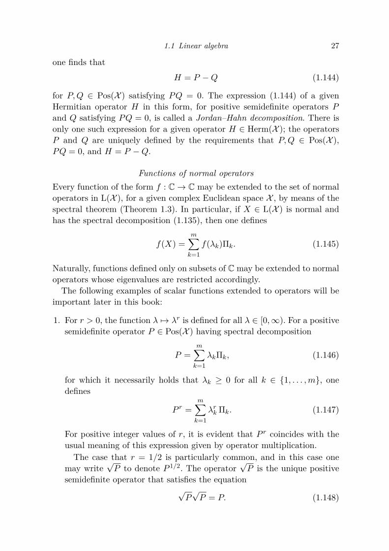
one finds thatH = P −Q (1.144)

for P,Q ∈ Pos(X ) satisfying PQ = 0. The expression (1.144) of a givenHermitian operator H in this form, for positive semidefinite operators Pand Q satisfying PQ = 0, is called a Jordan–Hahn decomposition. There isonly one such expression for a given operator H ∈ Herm(X ); the operatorsP and Q are uniquely defined by the requirements that P,Q ∈ Pos(X ),PQ = 0, and H = P −Q.

Functions of normal operatorsEvery function of the form f : C→ C may be extended to the set of normaloperators in L(X ), for a given complex Euclidean space X , by means of thespectral theorem (Theorem 1.3). In particular, if X ∈ L(X ) is normal andhas the spectral decomposition (1.135), then one defines

f(X) =m∑

k=1f(λk)Πk. (1.145)

Naturally, functions defined only on subsets of C may be extended to normaloperators whose eigenvalues are restricted accordingly.

The following examples of scalar functions extended to operators will beimportant later in this book:

1. For r > 0, the function λ 7→ λr is defined for all λ ∈ [0,∞). For a positivesemidefinite operator P ∈ Pos(X ) having spectral decomposition

P =m∑

k=1λkΠk, (1.146)

for which it necessarily holds that λk ≥ 0 for all k ∈ {1, . . . ,m}, onedefines

P r =m∑

k=1λrk Πk. (1.147)

For positive integer values of r, it is evident that P r coincides with theusual meaning of this expression given by operator multiplication.

The case that r = 1/2 is particularly common, and in this case onemay write

√P to denote P 1/2. The operator

√P is the unique positive

semidefinite operator that satisfies the equation√P√P = P. (1.148)


2. Along similar lines to the previous example, for any real number r ∈ R,the function λ 7→ λr is defined for all λ ∈ (0,∞). For a given positivedefinite operator P ∈ Pd(X ) having a spectral decomposition of the form(1.146), for which it holds that λk > 0 for all k ∈ {1, . . . ,m}, one definesP r in a similar way to (1.147) above.

3. The (base-2) logarithm function λ 7→ log(λ) is defined for all λ ∈ (0,∞).For a given positive definite operator P ∈ Pd(X ), having a spectraldecomposition (1.146) as above, one defines

log(P ) =m∑

k=1log(λk)Πk. (1.149)

The singular value theoremThe singular value theorem has a close relationship to the spectral theorem.Unlike the spectral theorem, however, the singular value theorem holds forarbitrary (nonzero) operators, as opposed to just normal operators.

Theorem 1.6 (Singular value theorem) Let A ∈ L(X ,Y) be a nonzerooperator having rank equal to r, for complex Euclidean spaces X and Y.There exist orthonormal sets {x1, . . . , xr} ⊂ X and {y1, . . . , yr} ⊂ Y, alongwith positive real numbers s1, . . . , sr, such that

A =r∑

k=1skykx

∗k. (1.150)

An expression of a given operator A in the form of (1.150) is said tobe a singular value decomposition of A. The numbers s1, . . . , sr are calledsingular values and the vectors x1, . . . , xr and y1, . . . , yr are called right andleft singular vectors, respectively.

The singular values s1, . . . , sr of an operator A are uniquely determined,up to their ordering. It will be assumed hereafter that singular values arealways ordered from largest to smallest: s1 ≥ · · · ≥ sr. When it is necessaryto indicate the dependence of these singular values on the operator A, theyare denoted s1(A), . . . , sr(A). Although 0 is not formally considered to be asingular value of any operator, it is convenient to also define sk(A) = 0 fork > rank(A), and to take sk(A) = 0 for all k ≥ 1 when A = 0. The notations(A) is used to refer to the vector of singular values

s(A) = (s1(A), . . . , sr(A)), (1.151)

or to an extension of this vector

s(A) = (s1(A), . . . , sm(A)) (1.152)


when it is convenient to view it as an element of Rm for m > rank(A).As suggested above, there is a close relationship between the singular

value theorem and the spectral theorem. In particular, the singular valuedecomposition of an operator A and the spectral decompositions of theoperators A∗A and AA∗ are related in the following way: it holds that

sk(A) =√λk(AA∗) =

√λk(A∗A) (1.153)

for 1 ≤ k ≤ rank(A), and moreover the right singular vectors of A areeigenvectors of A∗A and the left singular vectors of A are eigenvectors ofAA∗. One is free, in fact, to choose the left singular vectors of A to be anyorthonormal collection of eigenvectors of AA∗ for which the correspondingeigenvalues are nonzero—and once this is done the right singular vectors willbe uniquely determined. Alternately, the right singular vectors of A may bechosen to be any orthonormal collection of eigenvectors of A∗A for whichthe corresponding eigenvalues are nonzero, which uniquely determines theleft singular vectors.

In the special case that X ∈ L(X ) is a normal operator, one may obtaina singular value decomposition of X directly from a spectral decompositionof the form

X =n∑

k=1λkxkx

∗k. (1.154)

In particular, one may define S = {k ∈ {1, . . . , n} : λk 6= 0}, and set

sk = |λk| and yk = λk|λk|

xk (1.155)

for each k ∈ S. The expression

X =∑

k∈Sskykx

∗k (1.156)

then represents a singular value decomposition of X, up to a relabeling ofthe terms in the sum.

The following corollary represents a reformulation of the singular valuetheorem that is useful in some situations.

Corollary 1.7 Let X and Y be complex Euclidean spaces, let A ∈ L(X ,Y)be a nonzero operator, and let r = rank(A). There exists a diagonal andpositive definite operator D ∈ Pd(Cr) and isometries U ∈ U(Cr,X ) andV ∈ U(Cr,Y) such that A = V DU∗.


Polar decompositionsFor every square operator X ∈ L(X ), it is possible to choose a positivesemidefinite operator P ∈ Pos(X ) and a unitary operator W ∈ U(X ) suchthat the equation

X = WP (1.157)

holds; this follows from Corollary 1.7 by taking W = V U∗ and P = UDU∗.Alternatively, by similar reasoning it is possible to write

X = PW (1.158)

for a (generally different) choice of operators P ∈ Pos(X ) and W ∈ U(X ).The expressions (1.157) and (1.158) are known as polar decompositions of X.

The Moore–Penrose pseudo-inverseFor a given operator A ∈ L(X ,Y), one defines an operator A+ ∈ L(Y,X ),known as the Moore–Penrose pseudo-inverse of A, as the unique operatorthat possesses the following properties:

1. AA+A = A,2. A+AA+ = A+, and3. AA+ and A+A are both Hermitian.

It is evident that there is at least one such choice of A+, for if

A =r∑

k=1skykx

∗k (1.159)

is a singular value decomposition of a nonzero operator A, then

A+ =r∑

k=1

1skxky

∗k (1.160)

possesses the three properties listed above. One may observe that AA+ andA+A are projection operators, projecting onto the spaces spanned by theleft singular vectors and right singular vectors of A, respectively.

The fact that A+ is uniquely determined by the above equations may beverified as follows. Suppose that B,C ∈ L(Y,X ) both possess the aboveproperties:

1. ABA = A = ACA,2. BAB = B and CAC = C, and3. AB, BA, AC, and CA are all Hermitian.


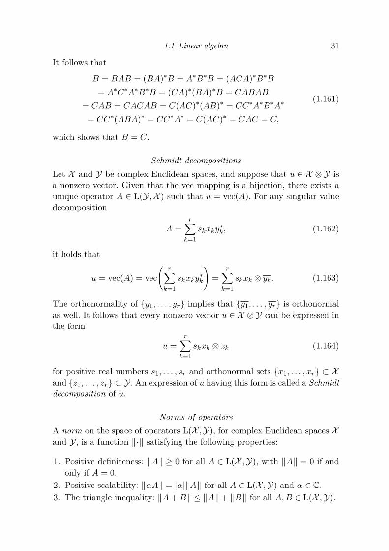
It follows that

B = BAB = (BA)∗B = A∗B∗B = (ACA)∗B∗B= A∗C∗A∗B∗B = (CA)∗(BA)∗B = CABAB

= CAB = CACAB = C(AC)∗(AB)∗ = CC∗A∗B∗A∗

= CC∗(ABA)∗ = CC∗A∗ = C(AC)∗ = CAC = C,

(1.161)

which shows that B = C.

Schmidt decompositionsLet X and Y be complex Euclidean spaces, and suppose that u ∈ X ⊗ Y isa nonzero vector. Given that the vec mapping is a bijection, there exists aunique operator A ∈ L(Y,X ) such that u = vec(A). For any singular valuedecomposition

A =r∑

k=1skxky

∗k, (1.162)

it holds that

u = vec(A) = vec(

r∑

k=1skxky

∗k

)=

r∑

k=1skxk ⊗ yk. (1.163)

The orthonormality of {y1, . . . , yr} implies that {y1, . . . , yr} is orthonormalas well. It follows that every nonzero vector u ∈ X ⊗ Y can be expressed inthe form

u =r∑

k=1skxk ⊗ zk (1.164)

for positive real numbers s1, . . . , sr and orthonormal sets {x1, . . . , xr} ⊂ Xand {z1, . . . , zr} ⊂ Y. An expression of u having this form is called a Schmidtdecomposition of u.

Norms of operatorsA norm on the space of operators L(X ,Y), for complex Euclidean spaces Xand Y, is a function ‖·‖ satisfying the following properties:

1. Positive definiteness: ‖A‖ ≥ 0 for all A ∈ L(X ,Y), with ‖A‖ = 0 if andonly if A = 0.

2. Positive scalability: ‖αA‖ = |α|‖A‖ for all A ∈ L(X ,Y) and α ∈ C.3. The triangle inequality: ‖A+B‖ ≤ ‖A‖+ ‖B‖ for all A,B ∈ L(X ,Y).


Many interesting and useful norms can be defined on spaces of operators,but this book will mostly be concerned with a single family of norms calledSchatten p-norms. This family includes the three most commonly used normsin quantum information theory: the spectral norm, the Frobenius norm, andthe trace norm.

For any operator A ∈ L(X ,Y) and any real number p ≥ 1, one defines theSchatten p-norm of A as

‖A‖p =(Tr((A∗A)

p2)) 1

p . (1.165)

The Schatten ∞-norm is defined as

‖A‖∞ = max {‖Au‖ : u ∈ X , ‖u‖ ≤ 1} , (1.166)

which coincides with limp→∞‖A‖p, explaining why the subscript ∞ is used.The Schatten p-norm of an operator A coincides with the ordinary vectorp-norm of the vector of singular values of A:

‖A‖p = ‖s(A)‖p. (1.167)

The Schatten p-norms possess a variety of properties, including the onessummarized in the following list:

1. The Schatten p-norms are non-increasing in p: for every operator A andfor 1 ≤ p ≤ q ≤ ∞, it holds that

‖A‖p ≥ ‖A‖q. (1.168)

2. For every nonzero operator A and for 1 ≤ p ≤ q ≤ ∞, it holds that

‖A‖p ≤ rank(A)1p− 1q ‖A‖q. (1.169)

In particular, one has

‖A‖1 ≤√

rank(A)‖A‖2 and ‖A‖2 ≤√

rank(A)‖A‖∞. (1.170)

3. For every p ∈ [1,∞], the Schatten p-norm is isometrically invariant (andtherefore unitarily invariant): for every A ∈ L(X ,Y), U ∈ U(Y,Z), andV ∈ U(X ,W) it holds that

‖A‖p = ‖UAV ∗‖p. (1.171)

4. For each p ∈ [1,∞], one defines p∗ ∈ [1,∞] by the equation1p

+ 1p∗

= 1. (1.172)


For every operator A ∈ L(X ,Y), it holds that the Schatten p-norm andp∗-norm are dual, in the sense that

‖A‖p = max{|〈B,A〉| : B ∈ L(X ,Y), ‖B‖p∗ ≤ 1

}. (1.173)

One consequence of (1.173) is the inequality

|〈B,A〉| ≤ ‖A‖p‖B‖p∗ , (1.174)

which is known as the Holder inequality for Schatten norms.5. For operators A ∈ L(Z,W), B ∈ L(Y,Z), and C ∈ L(X ,Y), and any

choice of p ∈ [1,∞], it holds that

‖ABC‖p ≤ ‖A‖∞‖B‖p‖C‖∞. (1.175)

It follows that the Schatten p-norm is submultiplicative:

‖AB‖p ≤ ‖A‖p‖B‖p. (1.176)

6. For every p ∈ [1,∞] and every A ∈ L(X ,Y), it holds that

‖A‖p =∥∥A∗

∥∥p

=∥∥AT∥∥

p=∥∥A∥∥p. (1.177)

The Schatten 1-norm is commonly called the trace norm, the Schatten2-norm is also known as the Frobenius norm, and the Schatten ∞-norm iscalled the spectral norm or operator norm. Some additional properties ofthese three norms are as follows:

1. The spectral norm. The spectral norm ‖·‖∞ is special in several respects.It is the operator norm induced by the Euclidean norm, which is itsdefining property (1.166). It also has the property that

‖A∗A‖∞ = ‖AA∗‖∞ = ‖A‖2∞ (1.178)

for every A ∈ L(X ,Y). Hereafter in this book, the spectral norm of anoperator A will be written ‖A‖ rather than ‖A‖∞, which reflects thefundamental importance of this norm.

2. The Frobenius norm. Substituting p = 2 into the definition of ‖·‖p, onesees that the Frobenius norm ‖·‖2 is given by

‖A‖2 =(Tr(A∗A)

) 12 =

√〈A,A〉, (1.179)

and is therefore analogous to the Euclidean norm for vectors, but definedby the inner product on L(X ,Y).


In essence, the Frobenius norm corresponds to the Euclidean norm ofan operator viewed as a vector:

‖A‖2 = ‖vec(A)‖ =√∑

a,b

∣∣A(a, b)∣∣2, (1.180)

where a and b range over the indices of the matrix representation of A.3. The trace norm. Substituting p = 1 into the definition of ‖·‖p, one has

that the trace norm ‖·‖1 is given by

‖A‖1 = Tr(√

A∗A), (1.181)

which is equal to the sum of the singular values of A. For two densityoperators ρ, σ ∈ D(X ), the value ‖ρ− σ‖1 is typically referred to as thetrace distance between ρ and σ.

A useful expression of ‖X‖1, for any square operator X ∈ L(X ), is

‖X‖1 = max{|〈U,X〉| : U ∈ U(X )

}, (1.182)

which follows from (1.167) and the singular value theorem (Theorem 1.6).As a result, one has that the trace-norm is non-increasing under theaction of partial tracing: for every operator X ∈ L(X ⊗Y), it holds that

‖TrY(X)‖1 = max{|〈U ⊗ 1Y , X〉| : U ∈ U(X )

}

≤ max{|〈V,X〉| : V ∈ U(X ⊗ Y)

}= ‖X‖1.

(1.183)

The identity∥∥αuu∗ − βvv∗

∥∥1 =

√(α+ β)2 − 4αβ|〈u, v〉|2, (1.184)

which holds for all unit vectors u, v and nonnegative real numbers α, β,is used multiple times in this book. It may be proved by considering thespectrum of αuu∗ − βvv∗; this operator is Hermitian, and has at mosttwo nonzero eigenvalues, represented by the expression

α− β2 ± 1

2

√(α+ β)2 − 4αβ |〈u, v〉|2. (1.185)

In particular, for unit vectors u and v, one has∥∥uu∗ − vv∗

∥∥1 = 2

√1− |〈u, v〉|2. (1.186)

1.2 Analysis, convexity, and probability theory 35

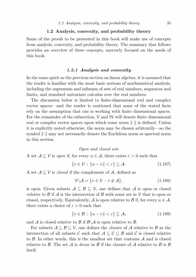
1.2 Analysis, convexity, and probability theorySome of the proofs to be presented in this book will make use of conceptsfrom analysis, convexity, and probability theory. The summary that followsprovides an overview of these concepts, narrowly focused on the needs ofthis book.

1.2.1 Analysis and convexityIn the same spirit as the previous section on linear algebra, it is assumed thatthe reader is familiar with the most basic notions of mathematical analysis,including the supremum and infimum of sets of real numbers, sequences andlimits, and standard univariate calculus over the real numbers.

The discussion below is limited to finite-dimensional real and complexvector spaces—and the reader is cautioned that some of the stated factsrely on the assumption that one is working with finite dimensional spaces.For the remainder of the subsection, V andW will denote finite dimensionalreal or complex vector spaces upon which some norm ‖·‖ is defined. Unlessit is explicitly noted otherwise, the norm may be chosen arbitrarily—so thesymbol ‖·‖ may not necessarily denote the Euclidean norm or spectral normin this section.

Open and closed setsA set A ⊆ V is open if, for every u ∈ A, there exists ε > 0 such that

{v ∈ V : ‖u− v‖ < ε

} ⊆ A. (1.187)

A set A ⊆ V is closed if the complement of A, defined as

V\A ={v ∈ V : v 6∈ A}, (1.188)

is open. Given subsets A ⊆ B ⊆ V, one defines that A is open or closedrelative to B if A is the intersection of B with some set in V that is open orclosed, respectively. Equivalently, A is open relative to B if, for every u ∈ A,there exists a choice of ε > 0 such that

{v ∈ B : ‖u− v‖ < ε

} ⊆ A; (1.189)

and A is closed relative to B if B\A is open relative to B.For subsets A ⊆ B ⊆ V, one defines the closure of A relative to B as the

intersection of all subsets C such that A ⊆ C ⊆ B and C is closed relativeto B. In other words, this is the smallest set that contains A and is closedrelative to B. The set A is dense in B if the closure of A relative to B is Bitself.


Continuous functionsLet f : A →W be a function defined on some subset A ⊆ V. For any vectoru ∈ A, the function f is said to be continuous at u if the following holds:for every ε > 0 there exists δ > 0 such that

‖f(v)− f(u)‖ < ε (1.190)

for all v ∈ A satisfying ‖u− v‖ < δ. If f is continuous at every vector in A,then one simply says that f is continuous on A.

For a function f : A → W defined on some subset A ⊆ V, the preimageof a set B ⊆ W is defined as

f−1(B) ={u ∈ A : f(u) ∈ B}. (1.191)

Such a function f is continuous on A if and only if the preimage of everyopen set in W is open relative to A. Equivalently, f is continuous on A ifand only if the preimage of every closed set in W is closed relative to A.

For a positive real number κ, a function f : A → W defined on a subsetA ⊆ V is said to be a κ-Lipschitz function if

‖f(u)− f(v)‖ ≤ κ‖u− v‖ (1.192)

for all u, v ∈ A. Every κ-Lipschitz function is necessarily continuous.

Compact setsA set A ⊆ V is compact if every sequence in A has a subsequence thatconverges to a vector u ∈ A. As a consequence of the fact V is assumed tobe finite dimensional, one has that a set A ⊆ V is compact if and only if itis both closed and bounded—a fact known as the Heine–Borel theorem.

Two properties regarding continuous functions and compact sets that areparticularly noteworthy for the purposes of this book are as follows:

1. If A is compact and f : A → R is continuous on A, then f achieves botha maximum and minimum value on A.

2. If A ⊂ V is compact and f : V → W is continuous on A, then

f(A) = {f(u) : u ∈ A} (1.193)

is also compact. In words, continuous functions always map compact setsto compact sets.


Differentiation of multivariate real functionsBasic multivariate calculus will be employed in a few occasions later in thisbook, and in these cases it will be sufficient to consider only real-valuedfunctions.

Suppose n is a positive integer, f : Rn → R is a function, and u ∈ Rn is avector. Under the assumption that the partial derivative

∂kf(u) = limα→0

f(u+ αek)− f(u)α

(1.194)

exists and is finite for each k ∈ {1, . . . , n}, one defines the gradient vector off at u as

∇f(u) =(∂1f(u), . . . , ∂nf(u)

). (1.195)

A function f : Rn → R is differentiable at a vector u ∈ Rn if there existsa vector v ∈ Rn with the following property: for every sequence (w1, w2, . . .)of vectors in Rn that converges to 0, one has that

limk→∞

|f(u+ wk)− f(u)− 〈v, wk〉|‖wk‖

= 0 (1.196)

(where here ‖·‖ denotes the Euclidean norm). In this case the vector v isnecessarily unique, and one writes v = (Df)(u). If f is differentiable at u,then it holds that

(Df)(u) = ∇f(u). (1.197)

It may be the case that the gradient vector ∇f(u) is defined for a vector uat which f is not differentiable, but if the function u 7→ ∇f(u) is continuousat u, then f is necessarily differentiable at u.

If a function f : Rn → R is both differentiable and κ-Lipschitz, then forall u ∈ Rn and for ‖·‖ denoting the Euclidean norm, it must hold that

‖∇f(u)‖ ≤ κ. (1.198)

Finally, suppose g1, . . . , gn : R → R are functions that are differentiableat a real number α ∈ R and f : Rn → R is a function that is differentiableat the vector (g1(α), . . . , gn(α)). The chain rule for differentiation impliesthat the function h : R→ R defined as

h(β) = f(g1(β), . . . , gn(β)) (1.199)

is differentiable at α, with its derivative being given by

h′(α) =⟨∇f(g1(α), . . . , gn(α)), (g′1(α), . . . , g′n(α))

⟩. (1.200)


NetsLet V be a real or complex vector space, let A ⊆ V be a subset of V, let ‖·‖be a norm on V, and let ε > 0 be a positive real number. A set of vectorsN ⊆ V is an ε-net for A if, for every vector u ∈ A, there exists a vectorv ∈ N such that ‖u − v‖ ≤ ε. An ε-net N for A is minimal if N is finiteand every ε-net of A contains at least |N | vectors.

The following theorem gives an upper bound for the number of elementsin a minimal ε-net for the unit ball

B(X ) = {u ∈ X : ‖u‖ ≤ 1} (1.201)

in a complex Euclidean space, with respect to the Euclidean norm.

Theorem 1.8 (Pisier) Let X be a complex Euclidean space of dimension nand let ε > 0 be a positive real number. With respect to the Euclidean normon X , there exists an ε-net N ⊂ B(X ) for the unit ball B(X ) such that

|N | ≤(

1 + 2ε

)2n. (1.202)

The proof of this theorem does not require a complicated construction;one may take N to be any maximal set of vectors chosen from the unit ballfor which it holds that ‖u − v‖ ≥ ε for all u, v ∈ N with u 6= v. Such aset is necessarily an ε-net for B(X ), and the bound on |N | is obtained bycomparing the volume of B(X ) with the volume of the union of ε/2 ballsaround vectors in N .

Borel sets and functionsThroughout this subsection, A ⊆ V and B ⊆ W will denote fixed subsets offinite-dimensional real or complex vector spaces V and W.

A set C ⊆ A is said to be a Borel subset of A if one or more of the followinginductively defined properties holds:

1. C is an open set relative to A.2. C is the complement of a Borel subset of A.3. For {C1, C2, . . .} being a countable collection of Borel subsets of A, it

holds that C is equal to the union

C =∞⋃

k=1Ck. (1.203)

The collection of all Borel subsets of A is denoted Borel(A).A function f : A → B is a Borel function if f−1(C) ∈ Borel(A) for allC ∈ Borel(B). That is, Borel functions are functions for which the preimage


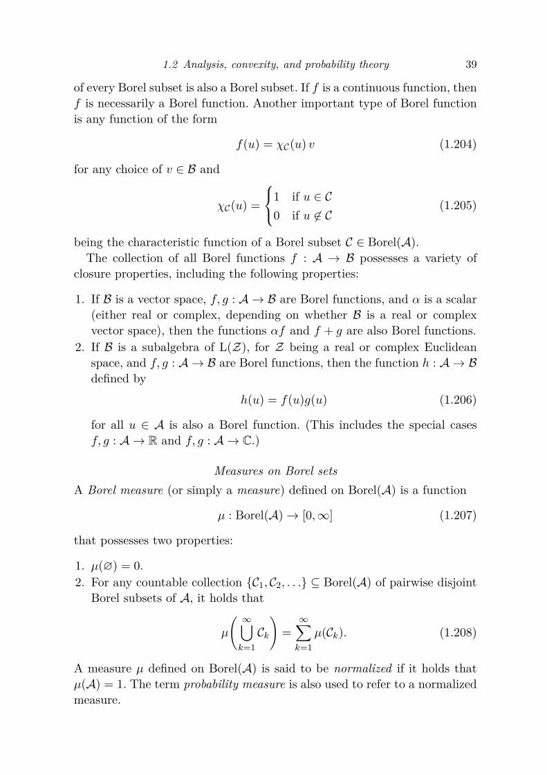
of every Borel subset is also a Borel subset. If f is a continuous function, thenf is necessarily a Borel function. Another important type of Borel functionis any function of the form

f(u) = χC(u) v (1.204)

for any choice of v ∈ B and

χC(u) =

1 if u ∈ C0 if u 6∈ C

(1.205)

being the characteristic function of a Borel subset C ∈ Borel(A).The collection of all Borel functions f : A → B possesses a variety of

closure properties, including the following properties:

1. If B is a vector space, f, g : A → B are Borel functions, and α is a scalar(either real or complex, depending on whether B is a real or complexvector space), then the functions αf and f + g are also Borel functions.

2. If B is a subalgebra of L(Z), for Z being a real or complex Euclideanspace, and f, g : A → B are Borel functions, then the function h : A → Bdefined by

h(u) = f(u)g(u) (1.206)

for all u ∈ A is also a Borel function. (This includes the special casesf, g : A → R and f, g : A → C.)

Measures on Borel setsA Borel measure (or simply a measure) defined on Borel(A) is a function

µ : Borel(A)→ [0,∞] (1.207)

that possesses two properties:

1. µ(∅) = 0.2. For any countable collection {C1, C2, . . .} ⊆ Borel(A) of pairwise disjoint

Borel subsets of A, it holds that

µ

( ∞⋃

k=1Ck)

=∞∑

k=1µ(Ck). (1.208)

A measure µ defined on Borel(A) is said to be normalized if it holds thatµ(A) = 1. The term probability measure is also used to refer to a normalizedmeasure.


There exists a measure ν defined on Borel(R), known as the standardBorel measure,3 that has the property

ν([α, β]) = β − α (1.209)

for all choices of α, β ∈ R with α ≤ β.If A1, . . . ,An are subsets of (not necessarily equal) finite-dimensional real

or complex vector spaces, and

µk : Borel(Ak)→ [0,∞] (1.210)

is a measure for each k ∈ {1, . . . , n}, then there is a uniquely defined productmeasure

µ1 × · · · × µn : Borel(A1 × · · · × An)→ [0,∞] (1.211)

for which

(µ1 × · · · × µn)(B1 × · · · × Bn) = µ1(B1) · · ·µn(Bn) (1.212)

for all B1 ∈ Borel(A1), . . . ,Bn ∈ Borel(An).

Integration of Borel functionsFor some (but not all) Borel functions f : A → B, and for µ being a Borelmeasure of the form µ : Borel(A)→ [0,∞], one may define the integral

∫f(u) dµ(u), (1.213)

which is an element of B when it is defined.An understanding of the specifics of the definition through which such

an integral is defined is not critical within the context of this book, butsome readers may find that a high-level overview of the definition is helpfulin associating an intuitive meaning to the integrals that do arise. In short,one defines what is meant by the integral of an increasingly large collectionof functions, beginning with functions taking nonnegative real values, andthen proceeding to vector (or operator) valued functions by taking linearcombinations.

1. Nonnegative simple functions. A function g : A → [0,∞) is a nonnegativesimple function if it may be written as

g(u) =m∑

k=1αk χk(u) (1.214)

3 The standard Borel measure agrees with the well-known Lebesgue measure on every Borelsubset of R. The Lebesgue measure is also defined for some subsets of R that are not Borelsubsets, which endows it with additional properties that happen not to be relevant withinthe context of this book.


for a nonnegative integer m, distinct positive real numbers α1, . . . , αm,and characteristic functions χ1, . . . , χm given by

χk(u) =

1 if u ∈ Ck0 if u 6∈ Ck

(1.215)

for disjoint Borel sets C1, . . . , Cm ∈ Borel(A). (It is to be understood thatthe sum is empty when m = 0, which corresponds to g being identicallyzero.)

A nonnegative simple function g of the form (1.214) is integrable withrespect to a measure µ : Borel(A) → [0,∞] if µ(Ck) is finite for everyk ∈ {1, . . . ,m}, and in this case the integral of g with respect to µ isdefined as

∫g(u) dµ(u) =

m∑

k=1αk µ(Ck). (1.216)

This is a well-defined quantity, by virtue of the fact that the expression(1.214) happens to be unique for a given simple function g.

2. Nonnegative Borel functions. The integral of a Borel function of the formf : A → [0,∞), with respect to a given measure µ : Borel(A) → [0,∞],is defined as ∫

f(u) dµ(u) = sup∫g(u) dµ(u), (1.217)

where the supremum is taken over all nonnegative simple functions of theform g : A → [0,∞) for which it holds that g(u) ≤ f(u) for all u ∈ A. Itis said that f is integrable if the supremum value in (1.217) is finite.

3. Real and complex Borel functions. A Borel function g : A → R isintegrable with respect to a measure µ : Borel(A)→ [0,∞] if there existintegrable Borel functions f0, f1 : A → [0,∞) such that g = f0 − f1, andin this case the integral of g with respect to µ is defined as

∫g(u) dµ(u) =

∫f0(u) dµ(u)−

∫f1(u) dµ(u). (1.218)

Similarly, a Borel function h : A → C is integrable with respect to ameasure µ : Borel(A) → [0,∞] if there exist integrable Borel functionsg0, g1 : A → R such that h = g0 + ig1, and in this case the integral of hwith respect to µ is defined as

∫h(u) dµ(u) =

∫g0(u) dµ(u) + i

∫g1(u) dµ(u). (1.219)


4. Arbitrary Borel functions. An arbitrary Borel function f : A → B isintegrable with respect to a given measure µ : Borel(A)→ [0,∞] if thereexists a finite-dimensional vector space W such that B ⊆ W, a basis{w1, . . . , wm} of W, and integrable functions g1, . . . , gm : A → R org1, . . . , gm : A → C (depending on whetherW is a real or complex vectorspace) such that

f(u) =m∑

k=1gk(u)wk. (1.220)

In this case, the integral of f with respect to µ is defined as∫f(u) dµ(u) =

m∑

k=1

(∫gk(u) dµ(u)

)wk. (1.221)

The fact that the third and fourth items in this list lead to uniquely definedintegrals of integrable functions is not immediate and requires a proof.

A selection of properties and conventions regarding integrals defined inthis way, targeted to the specific needs of this book, follows.

1. Linearity. For integrable functions f and g, and scalar values α and β,one has∫

(αf(u) + βg(u)) dµ(u) = α

∫f(u) dµ(u) + β

∫g(u) dµ(u). (1.222)

2. Standard Borel measure as the default. Hereafter in this book, wheneverf : R → R is an integrable function, and ν denotes the standard Borelmeasure on R, the shorthand notation

∫f(α) dα =

∫f(α) dν(α) (1.223)

will be used. It is the case that, whenever f is an integrable function forwhich the commonly studied Riemann integral is defined, the Riemannintegral will be in agreement with the integral defined as above for thestandard Borel measure—so this shorthand notation is not likely to leadto confusion or ambiguity.

3. Integration over subsets. For an integrable function f : A → B and aBorel subset C ∈ Borel(A), one defines

∫

Cf(u) dµ(u) =

∫f(u)χC(u) dµ(u), (1.224)


for χC being the characteristic function of C. The notationγ∫

β

f(α) dα =∫

[β,γ]

f(α) dα (1.225)

is also used in the case that f takes the form f : R → B and β, γ ∈ Rsatisfy β ≤ γ.

4. Order of integration. Suppose that A0 ⊆ V0, A1 ⊆ V1, and B ⊆ W aresubsets of finite-dimensional real or complex vector spaces, where it isto be assumed that V0 and V1 are either both real or both complex forsimplicity. If µ0 : Borel(A0) → [0,∞] and µ1 : Borel(A1) → [0,∞] areBorel measures, f : A0×A1 → B is a Borel function, and f is integrablewith respect to the product measure µ0×µ1, then it holds (by a theoremknown as Fubini’s theorem) that

∫ (∫f(u, v) dµ0(u)

)dµ1(v) =

∫f(u, v) d(µ0 × µ1)(u, v)

=∫ (∫

f(u, v) dµ1(v))

dµ0(u).(1.226)

Convex sets, cones, and functionsLet V be a vector space over the real or complex numbers. A subset C of Vis convex if, for all vectors u, v ∈ C and scalars λ ∈ [0, 1], it holds that

λu+ (1− λ)v ∈ C. (1.227)

Intuitively speaking, this means that for any two distinct elements u and v

of C, the line segment whose endpoints are u and v lies entirely within C.The intersection of any collection of convex sets is also convex.

If V and W are vector spaces, either both over the real numbers or bothover the complex numbers, and A ⊆ V and B ⊆ W are convex sets, then theset

{u⊕ v : u ∈ A, v ∈ B} ⊆ V ⊕W (1.228)

is also convex. Moreover, if A ∈ L(V,W) is an operator, then the set

{Au : u ∈ A} ⊆ W (1.229)

is convex as well.A set K ⊆ V is a cone if, for all choices of u ∈ K and λ ≥ 0, one has that

λu ∈ K. The cone generated by a set A ⊆ V is defined as

cone(A) ={λu : u ∈ A, λ ≥ 0}. (1.230)


If A is a compact set that does not include 0, then cone(A) is necessarily aclosed set. A convex cone is simply a cone that is also convex. A cone K isconvex if and only if it is closed under addition, meaning that u+ v ∈ K forevery choice of u, v ∈ K.

A function f : C → R defined on a convex set C ⊆ V is a convex functionif the inequality

f(λu+ (1− λ)v) ≤ λf(u) + (1− λ)f(v) (1.231)

holds for all u, v ∈ C and λ ∈ [0, 1]. A function f : C → R defined on aconvex set C ⊆ V is a midpoint convex function if the inequality

f(u+ v

2)≤ f(u) + f(v)

2 (1.232)

holds for all u, v ∈ C. Every continuous midpoint convex function is convex.A function f : C → R defined on a convex set C ⊆ V is a concave function

if −f is convex. Equivalently, f is concave if the reverse of the inequality(1.231) holds for all u, v ∈ C and λ ∈ [0, 1]. Similarly, a function f : C → Rdefined on a convex set C ⊆ V is a midpoint concave function if −f is amidpoint convex function, and therefore every continuous midpoint concavefunction is concave.

Convex hullsFor any alphabet Σ, a vector p ∈ RΣ is said to be a probability vector if itholds that p(a) ≥ 0 for all a ∈ Σ and

∑

a∈Σp(a) = 1. (1.233)

The set of all such vectors will be denoted P(Σ).For any vector space V and any subset A ⊆ V, a convex combination of

vectors in A is any expression of the form∑

a∈Σp(a)ua, (1.234)

for some choice of an alphabet Σ, a probability vector p ∈ P(Σ), and acollection

{ua : a ∈ Σ} ⊆ A (1.235)

of vectors in A.The convex hull of a set A ⊆ V, denoted conv(A), is the intersection of all

convex sets containing A. The set conv(A) is equal to the set of all vectorsthat may be written as a convex combination of elements of A. (This is true


even in the case that A is infinite.) The convex hull conv(A) of a closed setA need not itself be closed. However, if A is compact, then so too is conv(A).

The theorem that follows provides an upper bound on the number ofelements over which one must take convex combinations in order to generateevery point in the convex hull of a given set. The theorem refers to the notionof an affine subspace: a set U ⊆ V is an affine subspace of V having dimensionn if there exists a subspace W ⊆ V of dimension n and a vector u ∈ V suchthat

U = {u+ v : v ∈ W}. (1.236)

Theorem 1.9 (Caratheodory’s theorem) Let V be a real vector space andlet A be a subset of V. Assume, moreover, that A is contained in an affinesubspace of V having dimension n. For every vector v ∈ conv(A) in theconvex hull of A, there exist m ≤ n + 1 vectors u1, . . . , um ∈ A such thatv ∈ conv

({u1, . . . , um}).

Extreme pointsA point w ∈ C in a convex set C is said to be an extreme point of C if, forevery expression

w = λu+ (1− λ)v (1.237)

for which u, v ∈ C and λ ∈ (0, 1), it holds that u = v = w. In words, theextreme points are those elements of C that do not lie properly between twodistinct points of C.

The following theorem states that every convex and compact subset of afinite-dimensional vector space, over the real or complex numbers, is equalto the convex hull of its extreme points.

Theorem 1.10 (Minkowski) Let V be a finite-dimensional vector spaceover the real or complex numbers, let C ⊆ V be a compact and convex set,and let A ⊆ C be the set of extreme points of C. It holds that C = conv(A).

A few examples of convex and compact sets, along with an identificationof their extreme points, follow.

1. The spectral norm unit ball. For any complex Euclidean space X , the set{X ∈ L(X ) : ‖X‖ ≤ 1

}(1.238)

is a convex and compact set. The extreme points of this set are theunitary operators U(X ).


2. The trace norm unit ball. For any complex Euclidean space X , the set{X ∈ L(X ) : ‖X‖1 ≤ 1

}(1.239)

is a convex and compact set. The extreme points of this set are thoseoperators of the form uv∗ for u, v ∈ S(X ) unit vectors.

3. Density operators. For any complex Euclidean space X , the set D(X )of density operators acting on X is convex and compact. The extremepoints of D(X ) coincide with the rank-one projection operators. Theseare the operators of the form uu∗ for u ∈ S(X ) being a unit vector.

4. Probability vectors. For any alphabet Σ, the set of probability vectorsP(Σ) is convex and compact. The extreme points of this set are theelements of the standard basis {ea : a ∈ Σ} of RΣ.

Hyperplane separation and min-max theoremsConvex sets in real Euclidean spaces possess a fundamentally importantproperty: every vector lying outside of a given convex set in a real Euclideanspace can be separated from that convex set by a hyperplane. That is, if theunderlying real Euclidean space has dimension n, then there exists an affinesubspace of that space having dimension n− 1 that divides the entire spaceinto two half-spaces: one contains the convex set and the other containsthe chosen point lying outside of the convex set. The following theoremrepresents one specific formulation of this fact.

Theorem 1.11 (Hyperplane separation theorem) Let V be a real Euclideanspace, let C ⊂ V be a closed, convex subset of V, and let u ∈ V be a vectorwith u 6∈ C. There exists a vector v ∈ V and a scalar α ∈ R such that

〈v, u〉 < α ≤ 〈v, w〉 (1.240)

for all w ∈ C. If C is a cone, then v may be chosen so that (1.240) holds forα = 0.

Another theorem concerning convex sets that finds uses in the theory ofquantum information is the following theorem.

Theorem 1.12 (Sion’s min-max theorem) Let X and Y be real or complexEuclidean spaces, let A ⊆ X and B ⊆ Y be convex sets with B compact, andlet f : A× B → R be a continuous function such that

1. u 7→ f(u, v) is a convex function on A for all v ∈ B, and2. v 7→ f(u, v) is a concave function on B for all u ∈ A.


It holds thatinfu∈A

maxv∈B

f(u, v) = maxv∈B

infu∈A

f(u, v). (1.241)

1.2.2 Probability theoryConcepts from probability theory will play an important role throughoutmuch of this book. Probability distributions over alphabets or other finitesets will be viewed as having fundamental importance; they arise naturallywhen information-theoretic tasks and settings are considered. The reader isassumed to have familiarity with basic probability theory for distributionsover sets with finitely many elements. It will also be convenient to use thelanguage of probability theory to discuss properties of Borel measures.

Random variables distributed with respect to probability measuresSuppose A is a subset of a finite-dimensional real or complex vector spaceV and µ : Borel(A) → [0, 1] is a probability measure (by which it is meantthat µ is a normalized Borel measure). A random variable X distributedwith respect to µ is a real-valued, integrable Borel function of the form

X : A → R, (1.242)

which is typically viewed as representing an outcome of a random processof some sort.

For every Borel subset B ⊆ R of the real numbers, the probability that Xtakes a value in B is defined as

Pr(X ∈ B) = µ({u ∈ A : X(u) ∈ B}). (1.243)

As a matter of notational convenience, one often writes expressions such as

Pr(X ≥ β) and Pr(|X − β| ≥ ε), (1.244)

which are to be understood as meaning Pr(X ∈ B) for

B = {α ∈ R : α ≥ β} and B = {α ∈ R : |α− β| ≥ ε}, (1.245)

respectively. Other expressions of this form are interpreted in an analogousway.

The union bound states, for any random variable X and arbitrary Borelsubsets B1, . . . ,Bn of R, that

Pr(X ∈ B1 ∪ · · · ∪ Bn) ≤ Pr(X ∈ B1) + · · ·+ Pr(X ∈ Bn). (1.246)


The expected value (or mean value) of a random variable X, distributedwith respect to a probability measure µ : Borel(A)→ [0, 1], is defined as

E(X) =∫X(u) dµ(u). (1.247)

If X is a random variable taking nonnegative real values, then it holds that

E(X) =∞∫

0

Pr(X ≥ λ) dλ. (1.248)

Random variables for discrete distributionsFor a given alphabet Σ and a probability vector p ∈ P(Σ), one may alsodefine a random variable X, distributed with respect to p, in an analogousway to a random variable distributed with respect to a Borel measure. Inparticular, such a random variable is a function of the form

X : Σ→ R, (1.249)

and for every subset Γ ⊆ Σ one writes

Pr(X ∈ Γ) =∑

a∈Γp(a). (1.250)

In this case, the expected value (or mean value) of X is

E(X) =∑

a∈Σp(a)X(a). (1.251)

It is, in some sense, not necessary for random variables distributed withrespect to probability vectors of the form p ∈ P(Σ) to be viewed as beingfundamentally different from random variables distributed with respect toBorel probability measures. Indeed, one may consider the set

{1, . . . , n} ⊂ R, (1.252)

for some choice of a positive integer n, and observe that every subset of{1, . . . , n} is a Borel subset of this set. The Borel probability measures

µ : Borel({1, . . . , n})→ [0, 1] (1.253)

coincide precisely with the set of all probability vectors p ∈ P({1, . . . , n})through the equations

µ(B) =∑

b∈Bp(b) and p(a) = µ({a}), (1.254)

for every B ⊆ {1, . . . , n} and a ∈ {1, . . . , n}.


Thus, by associating an arbitrary alphabet Σ with the set {1, . . . , n}, onefinds that a random variable distributed with respect to a probability vectorp ∈ P(Σ) is represented by a random variable distributed with respect to aBorel probability measure.

Vector and operator valued random variablesIt is sometimes convenient to define random variables that take vector oroperator values, rather than real number values. Random variables of thissort will always be specified explicitly in terms of ordinary random variables(i.e., ones that take real values) in this book. For example, given randomvariables X1, . . . , Xn and Y1, . . . , Yn, for some choice of a positive integer n,one may refer to the vector-valued random variables

(X1, . . . , Xn) ∈ Rn and (X1 + iY1, . . . , Xn + iYn) ∈ Cn. (1.255)

The default meaning of the term random variable should be understood asreferring to real-valued random variables, and the term vector-valued randomvariable or operator-valued random variable will be used when referring torandom variables obtained in the manner just described.

Independent and identically distributed random variablesTwo random variables X and Y are said to be independent if

Pr((X,Y ) ∈ A× B) = Pr(X ∈ A) Pr(Y ∈ B) (1.256)

for every choice of Borel subsets A,B ⊆ R, and are said to be identicallydistributed if

Pr(X ∈ A) = Pr(Y ∈ A) (1.257)

for every Borel subset A ⊆ R. In general, these conditions do not requirethat X and Y are defined with respect to the same Borel measure. In bothcases, these notions may be extended to more than two random variables,as well as to vector-valued random variables, in a straightforward way.

Suppose that A is a subset of a finite-dimensional real or complex vectorspace, µ : Borel(A) → [0, 1] is a probability measure, and Y : A → R is arandom variable distributed with respect to µ. For any choice of a positiveinteger n, one may consider independent and identically distributed randomvariables X1, . . . , Xn, each being distributed in the same way as Y . For thepurposes of this book, one may assume without a loss of generality that thismeans that X1, . . . , Xn are Borel functions, taking the form

Xk : An → R (1.258)


and being defined asXk(u1, . . . , un) = Y (uk) (1.259)

for each k and each (u1, . . . , un) ∈ An. Moreover, each Xk is understood tobe distributed with respect to the n-fold product measure µ × · · · × µ onAn. In essence, this formal specification represents the simple and intuitivenotion that X1, . . . , Xn are uncorrelated copies of the random variable Y .

A few fundamental theoremsA few fundamental theorems concerning random variables will be used laterin this book. While these theorem do hold for more general notions of randomvariables, the theorem statements that follow should be understood to applyto random variables distributed with respect to Borel probability measures(including random variables distributed with respect to probability vectorsof the form p ∈ P(Σ) as a special case, as described above).

The first theorem to be stated in this subsection is Markov’s inequality,which provides a sometimes coarse upper bound on the probability that anonnegative random variable exceeds a given threshold value.

Theorem 1.13 (Markov’s inequality) Let X be a random variable takingnonnegative real values, and let ε > 0 be a positive real number. It holds that

Pr(X ≥ ε) ≤ E(X)

ε. (1.260)

The next theorem, known as Jensen’s inequality, concerns the expectedvalue of a convex function applied to a random variable.

Theorem 1.14 (Jensen’s inequality) Suppose that X is a random variableand f : R→ R is a convex function. It holds that

f(E(X)

) ≤ E(f(X)). (1.261)

Two additional theorems—known as the weak law of large numbers andHoeffding’s inequality—provide bounds on the deviation of the average valueof a collection of independent and identically distributed random variablesfrom their mean value.

Theorem 1.15 (Weak law of large numbers) Let X be a random variableand let α = E(X). Assume, moreover, for every positive integer n, thatX1, . . . , Xn are independent random variables identically distributed to X.For every positive real number ε > 0, it holds that

limn→∞Pr

(∣∣∣∣X1 + · · ·+Xn

n− α

∣∣∣∣ ≥ ε)

= 0. (1.262)


Theorem 1.16 (Hoeffding’s inequality) Let X1, . . . , Xn be independentand identically distributed random variables taking values in the interval[0, 1] and having mean value α. For every positive real number ε > 0 it holdsthat

Pr(∣∣∣∣X1 + · · ·+Xn

n− α

∣∣∣∣ ≥ ε)≤ 2 exp

(−2nε2). (1.263)

Gaussian measure and normally distributed random variablesThe standard Gaussian measure on R is the Borel probability measure

γ : Borel(R)→ [0, 1] (1.264)

defined as

γ(A) = 1√2π

∫

Aexp

(−α

2

2

)dα (1.265)

for every A ∈ Borel(R), where the integral is to be taken with respect to thestandard Borel measure on R. The fact that this is a well-defined measurefollows from the observation that the function

α 7→

1√2π exp

(−α2

2

)if α ∈ A

0 otherwise(1.266)

is an integrable Borel function for every Borel subset A ⊆ R, and the factthat it is a probability measure follows from the Gaussian integral

∫exp

(−α

2

2

)dα =

√2π. (1.267)

A random variable X is a standard normal random variable if it holdsthat Pr(X ∈ A) = γ(A) for every A ∈ Borel(R). This is equivalent to sayingthat X is identically distributed to a random variable Y (α) = α distributedwith respect to the standard Gaussian measure γ on R.

The following integrals are among many integrals of a similar sort thatare useful when reasoning about standard normal random variables:

1. For every positive real number λ > 0 and every real number β ∈ R itholds that

∫exp

(−λα2 + βα)

dα =√π

λexp

(β2

4λ

). (1.268)


2. For every positive integer n, it holds that∞∫

0

αn dγ(α) =2n2 Γ

(n+1

2)

2√π

, (1.269)

where the Γ-function may be defined at positive half-integer points asfollows:

Γ(m+ 1

2)

=

√π if m = 0

1 if m = 1m−1

2 Γ(m−1

2)

if m ≥ 2.(1.270)

3. For every positive real number λ > 0 and every pair of real numbersβ0, β1 ∈ R with β0 ≤ β1 it holds that

β1∫

β0

α exp(−λα2) dα = 12λ exp

(−λβ20)− 1

2λ exp(−λβ2

1). (1.271)

This formula also holds for infinite values of β0 and β1, with the naturalinterpretation exp(−∞) = 0.

For every positive integer n, the standard Gaussian measure on Rn is theBorel probability measure

γn : Borel(Rn)→ [0, 1] (1.272)

obtained by taking the n-fold product measure of γ with itself. Equivalently,

γn(A) = (2π)−n2

∫

Aexp

(−‖u‖

2

2

)dνn(u), (1.273)

where νn denotes the n-fold product measure of the standard Borel measureν with itself and the norm is the Euclidean norm.

The standard Gaussian measure on Rn is invariant under orthogonaltransformations (which include rotations):

γn(UA) = γn(A) (1.274)

for every Borel set A ⊆ Rn and every orthogonal operator U ∈ L(Rn),meaning one that satisfies UUT = 1. Therefore, for independent standardnormal random variables X1, . . . , Xn, one has that the vector valued randomvariable (X1, . . . , Xn) is identically distributed to the vector-valued randomvariable (Y1, . . . , Yn) obtained by defining

Yk =n∑

j=1U(k, j)Xj (1.275)


for each k ∈ {1, . . . , n}, for U ∈ L(Rn) being any orthogonal operator. As aconsequence of this fact, one has that if the standard Gaussian measure isprojected onto a subspace, it is equivalent to the standard Gaussian measureon that subspace.

Proposition 1.17 Let m and n be positive integers satisfying m < n andlet V ∈ L(Rm,Rn) satisfy V TV = 1. For every Borel set A ⊆ Rm, one has

γm(A) = γn({u ∈ Rn : V Tu ∈ A}). (1.276)

It follows from this proposition that the standard Gaussian measure γn(V)of any proper subspace V of Rn is zero.

Finally, for independent standard normal random variables X1, . . . , Xn,one may define a random variable

Y =√X2

1 + · · ·+X2n. (1.277)

The distribution of Y is known as the χ-distribution. The mean value of Yhas the following closed-form expression:

E(Y ) =√

2Γ(n+1

2)

Γ(n2) . (1.278)

From this expression, it may be proved that

E(Y ) = υn√n, (1.279)

where (υ1, υ2, . . .) is a strictly increasing sequence that begins

υ1 =√

2π, υ2 =

√π

2 , υ3 =√

83π , . . . (1.280)

and converges to 1 in the limit as n goes to infinity.

1.2.3 Semidefinite programmingThe paradigm of semidefinite programming finds numerous applications inthe theory of quantum information, both analytical and computational. Thissection describes a formulation of semidefinite programming that is well-suited to its (primarily analytical) applications found in this book.

Definitions associated with semidefinite programsLet X and Y be complex Euclidean spaces, let Φ ∈ T(X ,Y) be a Hermitian-preserving map, and let A ∈ Herm(X ) and B ∈ Herm(Y) be Hermitianoperators. A semidefinite program is a triple (Φ, A,B), with which thefollowing pair of optimization problems is associated:


Primal problem

maximize: 〈A,X〉subject to: Φ(X) = B,

X ∈ Pos(X ).

Dual problem

minimize: 〈B, Y 〉subject to: Φ∗(Y ) ≥ A,

Y ∈ Herm(Y).

With these problems in mind, one defines the primal feasible set A and thedual feasible set B of (Φ, A,B) as follows:

A ={X ∈ Pos(X ) : Φ(X) = B

},

B ={Y ∈ Herm(Y) : Φ∗(Y ) ≥ A}.

(1.281)

Operators X ∈ A and Y ∈ B are also said to be primal feasible and dualfeasible, respectively.

The function X 7→ 〈A,X〉, from Herm(X ) to R, is the primal objectivefunction, while the function Y 7→ 〈B, Y 〉, from Herm(Y) to R, is the dualobjective function of (Φ, A,B). The optimum values associated with theprimal and dual problems are defined as

α = sup{〈A,X〉 : X ∈ A} and β = inf

{〈B, Y 〉 : Y ∈ B}, (1.282)

respectively. (If it is the case that A = ∅ or B = ∅, then one defines α = −∞and β =∞, respectively.)

Semidefinite programming dualitySemidefinite programs have associated with them a notion of duality, whichrefers to the special relationship between the primal and dual problems.

The property of weak duality, which holds for all semidefinite programs,is that the primal optimum can never exceed the dual optimum. In moresuccinct terms, it necessarily holds that α ≤ β. This implies that every dualfeasible operator Y ∈ B provides an upper bound of 〈B, Y 〉 on the value〈A,X〉 that is achievable over all choices of a primal feasible X ∈ A, andlikewise every primal feasible operator X ∈ A provides a lower bound of〈A,X〉 on the value 〈B, Y 〉 that is achievable over all dual feasible operatorsY ∈ B.

It is not always the case that the primal optimum and dual optimum ofa semidefinite program (Φ, A,B) agree, but for many semidefinite programsthat arise naturally in applications, the primal optimum and dual optimumwill be equal. This situation is called strong duality. The following theoremprovides one set of conditions under which strong duality is guaranteed.


Theorem 1.18 (Slater’s theorem for semidefinite programs) Let X and Ybe complex Euclidean spaces, let Φ ∈ T(X ,Y) be a Hermitian-preservingmap, and let A ∈ Herm(X ) and B ∈ Herm(Y) be Hermitian operators.Letting A, B, α, and β be as defined above for the semidefinite program(Φ, A,B), one has the following two implications:

1. If α is finite and there exists a Hermitian operator Y ∈ Herm(Y) suchthat Φ∗(Y ) > A, then α = β, and moreover there exists a primal-feasibleoperator X ∈ A such that 〈A,X〉 = α.

2. If β is finite and there exists a positive definite operator X ∈ Pd(X ) suchthat Φ(X) = B, then α = β, and moreover there exists a dual-feasibleoperator Y ∈ B such that 〈B, Y 〉 = β.

In the situation that the optimum primal and dual values are equal, andare both achieved for some choice of feasible operators, a simple relationshipbetween these operators, known as complementary slackness, must hold.

Proposition 1.19 (Complementary slackness for semidefinite programs)Let X and Y be complex Euclidean spaces, let Φ ∈ T(X ,Y) be a Hermitian-preserving map, and let A ∈ Herm(X ) and B ∈ Herm(Y) be Hermitianoperators. Let A and B be the primal-feasible and dual-feasible sets associatedwith the semidefinite program (Φ, A,B), and suppose that X ∈ A and Y ∈ Bare operators satisfying 〈A,X〉 = 〈B, Y 〉. It holds that

Φ∗(Y )X = AX. (1.283)

Simplified forms and alternative expressions of semidefinite programsSemidefinite programs are typically presented in a way that is somewhatless formal than a precise specification of a triple (Φ, A,B), for Φ ∈ T(X ,Y)being a Hermitian-preserving map and A ∈ Herm(X ) and B ∈ Herm(Y)being Hermitian operators. Rather, the primal and dual problems are stateddirectly, often in a simplified form, and it is sometimes left to the readerto formulate a triple (Φ, A,B) that corresponds to the simplified problemstatements.

Two examples of semidefinite programs follow, in both cases includingtheir formal specifications and simplified forms.

Example 1.20 (Semidefinite program for the trace norm) Let X and Ybe complex Euclidean spaces and let K ∈ L(X ,Y) be any operator. Definea Hermitian-preserving map Φ ∈ T(X ⊕ Y) as

Φ(X ·· Y

)=(X 00 Y

)(1.284)


for all X ∈ L(X ) and Y ∈ L(Y), where the dots represent elements ofL(X ,Y) and L(Y,X ) that are effectively zeroed out by Φ. The map Φ isself-adjoint: Φ∗ = Φ. Also define A,B ∈ Herm(X ⊕ Y) as

A = 12

(0 K∗

K 0

)and B =

(1X 00 1Y

). (1.285)

The primal and dual problems associated with the semidefinite program(Φ, A,B) may, after some simplifications, be expressed as follows:

Primal problem

maximize: 12〈K,Z〉+ 1

2〈K∗, Z∗〉

subject to:(1X Z∗

Z 1Y

)≥ 0,

Z ∈ L(X ,Y).

Dual problem

minimize: 12 Tr(X) + 1

2 Tr(Y )

subject to:(X −K∗−K Y

)≥ 0,

X ∈ Pos(X ),Y ∈ Pos(Y).

The primal and dual optima are equal for all choices of K, and given by‖K‖1. (Given a singular value decomposition of K, one can construct botha primal feasible and dual feasible solution achieving this value.)

A standard way of expressing this semidefinite program would be to listonly the simplified primal and dual problems given above, letting the triple(Φ, A,B) be specified implicitly.

Example 1.21 (Semidefinite programs with inequality constraints) Let X ,Y, and Z be complex Euclidean spaces, let Φ ∈ T(X ,Y) and Ψ ∈ T(X ,Z)be Hermitian-preserving maps, and let A ∈ Herm(X ), B ∈ Herm(Y), andC ∈ Herm(Z) be Hermitian operators. Define a map

Ξ ∈ T(X ⊕ Z,Y ⊕ Z) (1.286)

as

Ξ(X ·· Z

)=(

Φ(X) 00 Ψ(X) + Z

)(1.287)

for all X ∈ L(X ) and Z ∈ L(Z). (Similar to the previous example, the dotsin the argument to Ξ represent arbitrary elements of L(X ,Z) and L(Z,X )upon which Ξ does not depend.) The adjoint map

Ξ∗ ∈ T(Y ⊕ Z,X ⊕ Z) (1.288)

1.3 Suggested references 57

to Ξ is given by

Ξ∗(Y ·· Z

)=(

Φ∗(Y ) + Ψ∗(Z) 00 Z

). (1.289)

The primal and dual problems of the semidefinite program specified bythe map Ξ, together with the Hermitian operators

(A 00 0

)∈ Herm(X ⊕ Z) and

(B 00 C

)∈ Herm(Y ⊕ Z), (1.290)

may be expressed in the following simplified form:

Primal problem

maximize: 〈A,X〉subject to: Φ(X) = B,

Ψ(X) ≤ C,X ∈ Pos(X ).

Dual problem

minimize: 〈B, Y 〉+ 〈C,Z〉subject to: Φ∗(Y ) + Ψ∗(Z) ≥ A,

Y ∈ Herm(Y),Z ∈ Pos(Z).

It is sometimes convenient to consider semidefinite programming problemsof this form, that include both equality and inequality constraints in theprimal problem, as opposed to just equality constraints.

1.3 Suggested referencesSeveral textbooks cover the material on linear algebra summarized in thischapter; the classic books of Halmos (1978) and Hoffman and Kunze (1971)are two examples. Readers interested in a more modern development oflinear algebra for finite dimensional spaces are referred to the book of Axler(1997). The books of Horn and Johnson (1985) and Bhatia (1997) also covermuch of the material on linear algebra that has been summarized in thischapter (and a great deal more, including relevant theorems to be provedin subsequent chapters of this book), with a focus on the matrix-theoreticaspects of the subject.

There are also many textbooks on mathematical analysis, including theclassic texts of Rudin (1964) and Apostol (1974), as well as the books ofBartle (1966) and Halmos (1974) that focus on measure theory. The book ofRockafellar (1970) is a standard reference on convex analysis, and the twovolume collection of Feller (1968, 1971) is a standard reference on probabilitytheory. Semidefinite programming is discussed by Wolkowicz, Saigal, andVandenberge (2000).

mathematical preliminaries - university of waterloowatrous/tqi/tqi.1.pdf · mathematical...

Documents