T L P

Mathematical Models in Municipal Solid Waste Management

M K. N

Department of Mathematical SciencesChalmers University of Technology and Goteborg University

Goteborg, Sweden

February 15, 2007

Mathematical Models in Municipal Solid WasteMichael K. Nganda

ISSN 1652-9715/NO 2007:6c©Michael K. Nganda, 2007Department of Mathematical Sciences

Chalmers University of Technology and Goteborg UniversitySE-412 96 Goteborg, SwedenTelephone:+46 (0)31 772 1000

Matematiskt CentrumJanuary 2007, Goteborg

Abstract

Two mathematical models developed as tools for solid waste planners in decisions concerning theoverall management of solid waste in a municipality are described. The models have respectivelybeen formulated as integer and mixed integer linear programming problems. The choice betweenthe two models from the practical point of view depends on theuser and the technology used.One user may prefer to measure the transportation costs in terms of costs per trip made fromthe waste source, in which case the first model is more appropriate. In this case we replace thecoefficients of the decision variables in the objective function with the total cost per trip fromthe waste collection point. At the same time, instead of measuring the amount of waste usingthe number of trucks used multiplied by their capacities, continuous variables can be introducedto measure directly the amount of waste that goes to the plants and landfills. The integer linearproblem is then transformed into a mixed integer problem that gives better total cost estimates andmore precise waste amount measurements, but measuring transportation costs in terms of costs pertrip. For instance, at the moment the first model is more relevant to the Ugandan situation, wherethe technology to measure waste as it is carried away from thewaste sources is not available.Another user may prefer to measure the transportation costsin terms of costs per unit mass ofwaste picked from the waste source, in which case the second model is more appropriate. Themodels allow to plan the optimal number of landfills and the treatment plants, and to determinethe optimal quantities and type of waste that has to be sent totreatment plants, to landfills and torecycling. It is also possible to determine the number and the type of trucks, as well as the numberand the type of replacement trucks and their depots. In either model there is one linear objective andlinear constraints that cover waste flows among the sources-plants-landfills, capacity, site selection,environmental, and facility availability. The objective function in either model describes tippingfees, total investment and maintenance costs, costs for buying/hiring trucks, transportation costsas well as operational costs from the use of replacement trucks. The benefits from refused derivedfuel, energy generation, compost, and recycling are also incorporated in the objective function.Validity and robustness tests conducted on the models, and applied on a hypothetical case studyare promising; the models can be used in important tools for planners in municipal solid wastemanagement in an urban environment. The models may as well beadapted for use in other areasof application like industrial warehouse location and product distributions among industry agents.

Acknowledgements

The content of this thesis was developed at the Department ofMathematical Sciences, ChalmersUniversity of Technology and Goteborg University, Goteborg, Sweden. I am very grateful to theteaching and non teaching staff of the department for the conducive working atmosphere withoutwhich it would have been impossible to attain this success. Their warm welcome will always beremembered.

I must also thank my fellow students like Konstantin Karagatsos that helped me very much as Istaggered in using Linux.

I must express my appreciation to the administrative staff like Martina Ramstedt and MarieKuhn for the friendly atmosphere that made it possible to complete my work there.

I give special thanks to the Medic staff for their continuous readiness to attend to my networkconnection queries.

In particular, the production of this work would have been invain without the inspired contri-bution of my supervisors Prof J. Bergh and Prof M. Patriksson.Their patience and understandingis particularly appreciated.

I am very grateful to the Department of Mathematics, Makerere University, Kampala, Ugandafor the support and encouragement in this academic adventure.

I highly value the financial support from the International Science Program (ISP), Uppsala,Sweden without which my studies at Chalmers would have been impossible. Special thanks goto Prof L. Abrahamsson, the coordinator of the East African Mathematics Program, and his entireteam at Uppsala.

I run short of words in expressing my gratitude to my dear wifeAnn for the unwavering supportand understanding she has always given and shown me, especially in the long periods of absencefrom home.

Contents

List of Figures ii

List of Tables iii

1 Introduction 11.1 Background to the study . . . . . . . . . . . . . . . . . . . . . . . . . . . . .. . 11.2 Statement of the Problem . . . . . . . . . . . . . . . . . . . . . . . . . . .. . . . 11.3 Objectives of the Study . . . . . . . . . . . . . . . . . . . . . . . . . . . .. . . . 21.4 Justification . . . . . . . . . . . . . . . . . . . . . . . . . . . . . . . . . . . .. . 3

2 Annotated Bibliography 3

3 Models of the Problem 93.1 First Model Formulation . . . . . . . . . . . . . . . . . . . . . . . . . . .. . . . 93.2 Analysis of the First Model . . . . . . . . . . . . . . . . . . . . . . . . .. . . . . 193.3 The Second Model of the Problem . . . . . . . . . . . . . . . . . . . . . .. . . . 203.4 Analysis of the Second Model . . . . . . . . . . . . . . . . . . . . . . . .. . . . 273.5 Examples illustrating how the Model Problems can be solved . . . . . . . . . . . . 27

3.5.1 An Integer Linear Model Example . . . . . . . . . . . . . . . . . . .. . . 273.5.2 A Mixed Integer Linear Model Example . . . . . . . . . . . . . . .. . . . 36

4 Case Study 414.1 Data used to test the Models . . . . . . . . . . . . . . . . . . . . . . . . .. . . . 424.2 Solution, Validity and Robustness of the First Model . . . .. . . . . . . . . . . . 454.3 Solution, Validity, and Robustness of the Second Model . .. . . . . . . . . . . . . 51

5 AMPL and CPLEX 565.1 Linear Programming . . . . . . . . . . . . . . . . . . . . . . . . . . . . . . .. . 565.2 Integer Programming . . . . . . . . . . . . . . . . . . . . . . . . . . . . . .. . . 56

6 Conclusions and future developments 57

i

List of Figures

1 A compact representation of key components in a decision support mathematicalmodel. . . . . . . . . . . . . . . . . . . . . . . . . . . . . . . . . . . . . . . . . . 2

2 A detailed representation of key components in a decision support mathematicalmodel. . . . . . . . . . . . . . . . . . . . . . . . . . . . . . . . . . . . . . . . . . 10

3 A simple model representation. . . . . . . . . . . . . . . . . . . . . . . .. . . . . 284 Second representation of the model. . . . . . . . . . . . . . . . . . . .. . . . . . 315 The third representation of the model. . . . . . . . . . . . . . . . . .. . . . . . . 326 The fourth representation of the model. . . . . . . . . . . . . . . . .. . . . . . . 347 Total costs plotted against the fractions of unrecovered waste . . . . . . . . . . . . 368 The fourth representation of the model. . . . . . . . . . . . . . . . .. . . . . . . 379 Total costs plotted against the fractions of unrecovered waste . . . . . . . . . . . . 4110 Total cost plotted against benefits from incineration . . .. . . . . . . . . . . . . . 4711 Total cost plotted against waste amount at Ntinda . . . . . . .. . . . . . . . . . . 4812 Total cost plotted against transportation costs from Kiwatule to Kiteezi . . . . . . . 4913 Total costs plotted against fractions of unrecovered waste . . . . . . . . . . . . . . 5014 Total cost plotted against benefits from incineration . . .. . . . . . . . . . . . . . 5215 Total cost plotted against waste amount at Ntinda . . . . . . .. . . . . . . . . . . 5316 Total cost plotted against transportation costs from Kiwatule to Kiteezi . . . . . . . 5417 Total costs plotted against fractions of unrecovered waste . . . . . . . . . . . . . . 55

ii

List of Tables

1 Total costs and fractions of unrecovered waste for the incinerator at node 2. . . . . 352 Total costs and fractions of unrecovered waste for the incinerator at node 2. . . . . 403 Node types and their locations . . . . . . . . . . . . . . . . . . . . . . . .. . . . 424 Waste amounts at waste sources. . . . . . . . . . . . . . . . . . . . . . . .. . . . 425 Capacities, costs of opening and waste handling, revenues from incinerators. . . . . 426 Landfill locations, landfill capacities, costs of opening landfills, and unit waste

handling charges. . . . . . . . . . . . . . . . . . . . . . . . . . . . . . . . . . . .437 Replacement trucks depot locations as well as their capacities and fixed costs in

opening them. . . . . . . . . . . . . . . . . . . . . . . . . . . . . . . . . . . . . . 438 Truck capacity, breakdown probability, and truck cost. . .. . . . . . . . . . . . . 439 Incinerator locations and waste proportions that remain at these incinerators. . . . . 4310 Transportation costs between waste sources and landfills. . . . . . . . . . . . . . . 4311 Expected number of trips a truck makes per day between a waste sources and a

landfills. . . . . . . . . . . . . . . . . . . . . . . . . . . . . . . . . . . . . . . . . 4412 Transportation costs between waste sources and incinerators. . . . . . . . . . . . . 4413 Expected number of trips a truck can make a day between a waste source and an

incinerator. . . . . . . . . . . . . . . . . . . . . . . . . . . . . . . . . . . . . . . 4414 Transportation costs between incinerators and landfills. . . . . . . . . . . . . . . . 4415 Expected number of trips a truck can make a day between an incinerator and a

landfill. . . . . . . . . . . . . . . . . . . . . . . . . . . . . . . . . . . . . . . . . 4416 Transportation costs between replacement trucks depotsand landfills. . . . . . . . 4517 Transportation costs between replacement trucks depotsand incinerators. . . . . . 4518 Transportation costs between replacement trucks depotsand waste sources. . . . . 4519 Total costs and benefits from Kiwatule. . . . . . . . . . . . . . . . .. . . . . . . . 4720 Total costs and waste amounts at Ntinda. . . . . . . . . . . . . . . .. . . . . . . . 4821 Total costs and transportation costs from Kiwatule wastesource to Kiteezi landfill. 4922 Total costs and fractions of unrecovered waste at incinerators . . . . . . . . . . . . 5023 Total costs and benefits from Kiwatule. . . . . . . . . . . . . . . . .. . . . . . . . 5124 Total costs and waste amounts at Ntinda. . . . . . . . . . . . . . . .. . . . . . . . 5225 Total costs and transportation costs from Kiwatule wastesource to Kiteezi landfill. 5326 Total costs and fractions of unrecovered waste at the incinerators . . . . . . . . . . 54

iii

List of Acronyms

1. MSW= municipal solid waste

2. RDF= refuse derived fuel

3. SWM= solid waste management

4. SOM= stabilized organic material

iv

1 Introduction

1.1 Background to the study

The protection of the environment and natural resources is increasingly becoming very impor-tant through environmentally sustainable waste management programs. It is necessary to follow,on the part of waste managers, a sustainable approach to waste management and to integrate strate-gies that will produce the best practicable option. This is avery challenging task since it involvestaking into account economic, technical, regulatory (normative), and environmental issues (Costiet al [18]). Waste management can become more complex if social and political considerations arealso taken into account.

Municipal solid waste (MSW) management involves the collection of waste from its sources andthe transportation of waste to processing plants where it can either be converted into fuel (refusederived fuel), electrical energy, compost (stabilised organic material) or recycled for reuse. Theunrecoverable waste can either be transported directly from the waste sources to landfills or fromtreatment plants to landfills. A careful planning is required in order to execute these activities in anoptimal way. Municipal solid waste has several sources suchas residential areas, commercial areas,institutional environments, construction and demolitionareas, municipal services, etc. (Badran andEl-Haggar [3]).

1.2 Statement of the Problem

Kampala, the capital city of Uganda, has a population of morethan one million people, and it isestimated that more than one thousand tons of MSW is generated per day. About half of the wastegenerated is collected and disposed of at the only landfill atKiteezi. Limited treatment is done atthe landfill where some organic material is converted into compost; this is done in order to save thewater streams near the landfill. A limited amount of waste is picked by individuals that sell it tosome industries for reuse as raw material; this covers plastic bottles, tins and other metallic objects.A limited amount of organic material is also picked by individuals as animal feeds to cattle, pigsand dogs. Since less than half of the waste is collected and the waste is in the open, much of itlitters the city whenever the wind blows and whenever it rains. This explains the incidence of theannual cholera outbreaks during the rainy seasons and the terrible stench from the city areas wherethe waste accumulated has decayed.

Until recently, the City Council of Kampala has been the sole body dealing with waste man-agement in the entire city. Privatization has now taken place and Kampala City Council plays theoverall supervisory role of making sure that the private companies follow the agreements madewith it. The city is currently composed of six divisions and there may be more than one companyin a single division. These companies are still in their infant stage and they currently collect andtransport MSW to the single landfill at Kiteezi. Optimization of solid waste management basedon operations research techniques has not yet been applied by any of the private companies. Atthe moment none of the companies treats waste and the decisions are basically based on intuitionand experience. There is an urgent need to utilize scientifictechniques as decision support toolsin order to provide a healthy environment to all city dwellers and to optimally use the availableresources in the day to day management of waste.

1

1.3 Objectives of the Study

The aim of this work is to present a detailed description of the mathematical models that can beused as tools for decision makers of a municipality in the dayto day planning and management ofintegrated programs of solid waste collection, incineration, recycling, treatment, and disposal. Themodels can as well be used as design tools for the plants, landfills, and truck depots, in addition tothe day to day planning of municipal solid waste. The main focus of the models, whose structuresare described in this thesis, is to plan the MSW management, by defining the refuse flows thathave to be sent to recycling or to different treatment plants or landfills, suggesting the number,the types, and the selection of plants or landfills that have to remain active at minimum total cost.Several treatment plants and facilities will be included within the desired MSW mathematicalmodel: trucks for the transportation of waste, plants for recycling, production of refuse derivedfuel (RDF), and treatment of organic material; incineratorswith energy recovery; sanitary landfills;standby trucks and their depots.

The application of the models may take some time as it may involve testing the models, andthe companies managing waste may need some time to implementthe proposals in the modelslike setting up plants. The proposed models may as well undergo some modifications since almostall companies managing waste in the city have small financialbudgets. What is likely to emergewith time are companies that only collect and transport waste, companies that only treat waste,and companies that only manage landfills. The models will however be a good starting pointtowards a sustainable municipal solid waste management andan understanding of integral wastemanagement as a way of shaping the direction of municipal solid waste management in Ugandancities or towns.

Figure 1 shows a compact representation of the key components of the models where the nodesstand for waste source locations (collection points), sanitary landfills, processing plants, and re-placement trucks depot locations. The arrows from the truckdepots node to the other three nodesindicate the flow of replacement trucks to those nodes. The arrows among waste sources, landfills,and processing plants nodes indicate the flow of waste among these nodes.'

&$%

'&

$%

'&

$%

'&

$%

?

-

6

I

ll

ll

lll

waste sources

landfills truck depots

processingplants

Figure 1: A compact representation of key components in a decision support mathematical model.

2

1.4 Justification

Waste management is very important for every country since it directly affects the health of herpeople and their environment. For example in Uganda choleraoutbreaks are common in congestedareas, especially during the rainy season. It is imperativethat efficient municipal solid wastemanagement methods are put in place. Municipal solid waste also serves as an ambit for diseasevectors like rodents. Eutrophication, the increased presence of nutrients and its consequence hasbeen one of the most serious lake water quality problems overthe last decades. By allowing therotting municipal waste to enter water channels to our rivers and lakes, we risk losing our watersources and fish because a fertile ground for water hyacinth and other water plants is generated.This too impairs the health and the economic power of the state - wetlands that are so importantfor a healthy environment are also affected by such waste. Noxious gases from rotting garbagealso end up in the atmosphere and can be deadly to human, animal, and plant life. With populationgrowth the land for waste disposal and agricultural production becomes scarce, and since it takeslong to reclaim land that has once been used for waste disposal, it becomes crucial to put in placemechanisms for reducing waste to landfills.

A brief survey of the main approaches proposed in the literature for solid waste management(SWM) models, during the last two decades, is made in Section 2. Section 3 discusses the math-ematical modelling of the municipal solid waste managementproblem. The model formulationsare described in Sections 3.1 and 3.3 while the analyses of the models are outlined in Sections3.2 and Section 3.4. The case study through which the validity and robustness of the models aretested is described in Section 4. The examples used to illustrate how the models can be solved aregiven in Section 3.5. The data used in the case study is presented in Section 4.1 while the resultsfrom the validity and robustness tests of the models are discussed in Sections 4.2 and 4.3. Theprogramming language and the solver used are briefly described in Section 5. The conclusions andfuture developments are presented in Section 6.

2 Annotated Bibliography

The effective application of SWM mathematical models as tools for decision making by munic-ipal solid waste planners, in developing countries, is still a big challenge. A considerable amountof research has been done in the last two decades on various aspects of SWM, and a number of eco-nomically based optimization models for waste streams allocation and collection vehicle routes,have been developed. Owing to an increasing awareness of environmental protection and con-servation of natural resources, rising prices of raw materials, and energy conservation concerns,the current research in SWM is now guided by the aim of designing comprehensive models thattake into account multi-disciplinary aspects involving economic, technical, regulatory, and envi-ronmental sustainability issues.

The solid waste models that have been developed in the last two decades have varied in goalsand methodologies. Solid waste generation prediction, facility site selection, facility capacity ex-pansion, facility operation, vehicle routing, system scheduling, waste flow and overall systemoperation, have been some of these goals (Badran and El-Haggar [3]).

Some of the techniques that have been used include linear programming, integer programming,mixed integer programming, non-linear programming, dynamic programming, goal programming,grey programming, fuzzy programming, quadratic programming, stochastic programming, two-stage programming, and interval-parameter programming, geographic information systems (Ghoseet al [24] and Hasit Warner [27]).

3

The main objective of most of the models developed has been tominimize cost. Some modelsare dynamic, while others are static (Badran and EL-Haggar [3]). Morrissey and Browne [49]have classified municipal waste management models into three categories on the basis of decisionmaking criteria: cost benefit analysis, life cycle analysis, and multi-criteria decision making.

A detailed description of the mathematical models that havemost inspired the development ofthe models presented in Section 3 is made below, while the other relevant and interesting modelsare mentioned at the end of this section.

Costi et al [18] have proposed a mixed integer nonlinear programming decision support modelto help decision makers of a municipality in the developmentof incineration, disposal, treatment,and recycling integrated programs. In that model several treatment plants and facilities have beenconsidered: separators, plants for producing refuse derived fuel (RDF), incinerators with energyrecovery, plants for treatment of organic material, and sanitary landfills. The main objective of thatmodel is to plan the municipal solid waste (MSW) management, define the refuse flow that hasto be sent to recycling or to different treatment or disposal landfills, and to determine the optimalnumber, the kinds, and the localization of the plants that are to be active. Some of the decisionvariables in the model are binary while others are continuous. The objective consists of all possibleeconomic costs and subjected to technical, regulatory (normative), and environmental constraints.In particular, pollution and impacts induced by the overallsolid waste management system, areconsidered through the formalization of constraints on incineration, emissions and on negativeeffects produced by disposal or other forms of treatments like RDF chemical composition. A casestudy, relevant to the municipality of Genova, Italy, has been presented.

Fiorucci et al [22] have presented a mixed integer nonlinearprogramming decision supportmodel for assisting planners in decisions regarding the overall management of solid waste at amunicipal level. By using that model, an optimal number of landfills and treatment plants, optimalquantities and the characteristics of refuse that have to besent to treatment plants, to landfills andto recycling can be determined. Various classes of constraints are considered in the problem for-mulation, considering the regulations about the minimum requirements for recycling, incinerationprocess requirements, sanitary landfill conservation, andmass balance. The objective function iscomposed of recycling, transportation and maintenance costs. The model has been tested on themunicipality of Genova, Italy. Unlike Costi et al [18], Fiorucci et al [22], have not considered con-straints associated with the environmental impact due to incineration, production of refuse derivedfuel (RDF), or stabilized organic material (SOM).

Badran and El-Haggar [3] have proposed a mixed integer linearprogramming model for theoptimal management of municipal solid waste at Port Said, Egypt. The idea is to choose a com-bination of collection stations from the possible locations in such a way as to minimize the dailytransportation costs from the districts to the collection stations, from the collection stations tocomposting plants and landfills, and from the collection stations to landfills. The constraints of thesingle objective (i.e. total cost) are the capacity constraints for the collection stations, compost-ing plants, and landfills. The model tests show positive results that can result in profit from thecollection fees and the sales of sorted recyclable material.

Daskalopoulos et al [19] have presented a mixed integer linear programming model for the man-agement of MSW streams, taking into account their rates and compositions, as well as their adverseenvironmental impacts. Using this model, they identify theoptimal combination of technologiesfor handling, treatment and disposal of MSW in a better economical and more environmentallysustainable way. The single objective is composed of costs per tonne of waste treated at the recy-cling, composting, incinerating plants, and landfills. Theconstraints of the objective are capacityconstraints for the plants and landfills. The model has been applied to the management of MSW

4

in the UK. The findings have revealed that the current costs favour the landfill option of managingthe MSW. It is however noted that the impact of a potential levy on waste land filled, can reducethe gap between the costs of land filling and the other alternative waste-treatment technologies.

Chang and Chang [6] have presented a non-linear programming model for municipal solid wastemanagement based on the minimization of an overall cost considering energy and material recoveryrequirements. A set of continuous decision variables that express material flows to the variousfacilities are defined. Presorting facilities (separators) are part of the model. The objective functionincludes transportation, treatment, and fixed and operational costs, and takes into account possiblebenefits from the sale of electric energy and recyclable raw materials. The problem constraintscover mass balance, incinerator and landfill capacities, and minimum energy recovery constraints.The proposed model has been tested in the Taipei metropolitan region, Taiwan. The tests areencouraging.

Similarities and differences between the current work and the foregoing lit-erature survey

Costi et al [18] have presented a comprehensive mixed integernonlinear programming problem,whose planning horizon is a year. They give a detailed description of environmental constraintsthat cover RDF constraints, incineration constraints, and SOM constraints.

The nonlinearity of their model consists in the nature of thedecision variables used. Thesedecision variables are percentages (fractions) of waste that has to be sent to various plants andlandfills in their model. The interaction between these percentages generates their products thatappear in the objective function, in the regulatory (normative) constraints, in the technical andenvironmental constraints. Probably the choice of the variables is due to the desired goal, andconsequently nonlinearity is inevitable. Transformationto a linear model may require change ofvariables.

In contrast to the work of Costi et al [18], we present two models; the first model is an integerlinear programming problem. Some of the variables in this model measure the number of trucks(including replacement trucks) used per day. The amount of waste transported is then determinedby multiplying the number of trucks of a given type used between any two nodes by the capacityof a single truck, and by the expected number of trips a singletruck of that type makes per daybetween those nodes. The binary variables used in the model decide the existence of a plant of agiven type, and a landfill of a given type or size.

The second model is a mixed integer linear programming problem where the continuous vari-ables measure the amount of waste that flows between the nodeswhile the integer variables mea-sure the number of trucks used per day. The binary variables,like in the first model, decide theexistence of a plant or a landfill.

We have two models because of the realization that some usersmay want to measure transporta-tion costs in terms of costs per trip from a waste collection point, in which case the first model ismore appropriate. Others may prefer to measure the transportation costs in terms of costs per unitwaste carried away from a waste collection point, in which case the second model is more appro-priate. For instance, the first model is more desirable for the Ugandan situation since it is not yetpossible to measure waste as it is transported from the wastecollection points.

The planning horizon in both models is a day; decisions are tobe taken on a day to day ba-sis. This means a continuous monitoring and collection of data in order to make the requiredadjustments. This flexibility may be lost in a long period horizon model. In addition to the dailyoperational utility of the models, they can as well be used asdesign tools for the plants, landfills,

5

and truck depots. Apart from the transportation costs, installation and operational costs for plantsand landfills, and benefits from recycling, RDF sales, SOM sales, and energy sales, the objectivefunction also includes truck purchase costs as well as costsdue to the presence of replacementtrucks depots.

Since our desire is not only that of locating plants and deciding waste flows to these plants andlandfills, special attention has been given to deciding the number and the type of trucks that areused to transport a given type of waste from the waste collection points to the plants or landfills.Replacement trucks are also considered with the observationof possible breakdowns of the opera-tional trucks. This is an aspect that is missing in the surveyed works, and since transportation costsplay a big part in the daily operational costs, it is important that a waste management planner hasa tool as a basis for the trucks deployed.

Although regulatory, technical, and environmental constraints are not comprehensively consid-ered in our models as by Costi et al [18] and Fiorucci et al [22],it is our belief that they can behandled in detail without affecting the linearity of the models. The regulatory constraints givethe minimum percentage of waste recycling; these percentages are proportions of the total wastegenerated. The technical constraints not only deal with plant capacities but also deal with theminimum amount of waste that has to be sent to the plants if these plants are to be economicallybeneficial. The environmental constraints are necessary tolimit emissions during the combustionprocesses at incinerators, and to limit the presence of noxious substances in the RDF and in theSOM. Along the same line leachate and biogas production at landfills can be studied.

Unlike in the model of Costi et al [18], waste flows from RDF, recycling, and SOM plants toincinerators are not considered in our models. These are left out in order to first develop the keyelements that deal with the determination of trucks used in the daily transportation exercise. Thesemissing elements can however be incorporated by defining newsets of variables to cover the wasteflows from the RDF plants, from the recycling plants, and from the SOM plants to the incinerators,since the aim is to recover as much waste as possible.

One similarity between our models and that of Costi et al [18] is that collection costs from wastesources to collection points are not part of the models. Other similarities are that our models areall static and deterministic (Murty [51]), and single objectives that minimize total costs are used.A major similarity is that the goal is to present integrated models that are comprehensive.

The model of Fiorucci et al [22] can be derived from that of Costi et al [18] by ignoring environ-mental constraints. Like in the model of Costi et al [18], the nonlinearity of their model consistsin the nature of the decision variables used. These decisionvariables are percentages (fractions)of waste that has to be sent to various plants and landfills in their model. The interaction betweenthese percentages generates their products that appear in the objective function, in the regulatory(normative) constraints, and in the technical constraints.

The model of Chang and Chang [6] minimizes overall cost (takinginto account energy and ma-terial recovery) through the solution of a nonlinear programming problem. Unlike Costi et al [18],their model does not cater for regulatory and environmentalconstraints while technical constraintsare not as extensively described as done by Costi et al [18]. Wepresent linear models, and go atlength in dealing with the waste transportation by determining the truck types and numbers as wellas considering replacement trucks in our models. We also show environmental constraints can beincluded.

Badran and El-Haggar [3] present a mixed integer linear programming model whose objectivecovers collection costs from the districts to collection stations, transportation costs from collectionstations to either composting plants or to landfills. Benefitsfrom the sale of compost and recy-clable material are incorporated into the objective function. Binary variables are used to decide the

6

existence of collection stations. Incineration, recycling, and RDF production are not part of themodel. Regulatory, technical, and environmental constraints are not covered in the model. UnlikeBadran and El-Haggar [3], waste collection from the sources of generation is not considered in ourmodels, and collection points are assumed to be known. Recycling, refused derived fuel, and en-ergy generation are considered in our models. The determination of trucks as well as replacementtrucks used everyday is not considered by Badran and El-Haggar [3]. Our models are linear liketheir model.

The model of Daskalopoulos et al [19] does not cover collection and transportation costs. Reg-ulatory and technical constraints are not considered either. The costs in the objective function caterfor the environmental considerations related to the emission of greenhouse gases. These costs areevaluated by costing all possible environmental damages that are associated with the waste man-agement options, like potential crop yield reduction, forest damage, sea level rise, and damage tohuman health. Unlike our models where several aspects of waste management planning are consid-ered, the model of Daskalopoulos [19] is restricted to wastetreatment and environmental impact.Such a model can be useful to companies that solely deal with municipal solid waste treatment. Itcan also be expanded to cater for the missing elements.

ReVelle [53] presents a survey on the applications of operations research to a variety of envi-ronmental problem areas like water resource management, water quality management, solid wasteoperation and design, cost allocation for environmental facilities, and air quality management. Henotes that despite four decades of such activities, challenging operational research problems stillremain in all of those areas. The open problems described include the design of rationing strategiesin a system of parallel reservoirs, hydro power production planning, simultaneous siting and effi-ciency determination of waste water treatment plants, design of the sequence of facilities in solidwaste collection/disposal system, the achievement of equity as well as rationality in cost alloca-tion, the planning of cost allocation when demands change over time, and the siting of air qualitymonitoring stations.

The other relevant solid waste management models are outlined below under the followingseven distinct traits:

1) Linear models; 2) Nonlinear models; 3) Dynamic models; 4)Static models; 5) Stochastic mod-els; 6) Deterministic models; 7) Multi-objective models; 8) Single objective models.

The models under trait one include Badran and El-Haggar [3], Daskalopoulos et al [19], Alidi[1], Amouzegar and Moshirvaziri [2], Bloemhof-Ruwaard et al [4], Caruso et al [5], Chang et al[7], Chang and Davila [9], Chang et al [11], Chang et al [12], Changand Wang [13], Chang andWang [14], Chang and Wang [15], Chang and Wang [17], Davila and Chang [20], Everett andModak [21], Gottinger ([25], [26]), Huang et al [28], Huang et al [29], Huang et al [30], Huang etal [32], Huang et al [33], Huang et al [34], Huang et al [35], Huang et al [37], Huang et al [38],Huang et al [39], Hsin-Neng and Kuo-hua [40], Kuhner and Harrington [42], Kulcar [43], Li andHuang [44], Li et al [45], Maqsood and Huang [46], Marks and Liebman [47], Nie et al [52], andSolano et al ([54], [55]).

Under trait two there is Costi et al [18], Fiorucci et al [22], Chang and Chang et al [6], Changet al [8], Chang and Wang [16], Huang et al [31], Huang et al [36], Minciardi et al [48], and Wu etal [57].

In trait three there is Chang et al [11], Chang et al [12], Chang and Wang [13], Chang and Wang[15], Huang et al [32], Huang et al [34], and Kuhner and Harrington [42].

Trait four comprises Costi et al [18], Fiorucci et al [22], Daskalopoulos et al [19], Alidi [1],

7

Amouzegar and Moshirvaziri [2], Badran and El-Haggar [3], Bloemhof-Ruwaard et al [4], Carusoet al [5], Chang and Chang et al [6], Chang et al [7], Chang et al [8],Chang and Davila [9], Changand Wang [14], Chang and Wang [16], Chang and Wang [17], Davila and Chang [20], Everett andModak [21], Gottinger ([25], [26]), Huang et al [28], Huang et al [29], Huang et al [30], Huang etal [31], Huang et al [33], Huang et al [35], Huang et al [36], Huang et al [37], Huang et al [38],Huang et al [39], Hsin-Neng and Kuo-hua [40], Kuhner and Harrington [42], Kulcar [43], Li andHuang [44], Li et al [45], Maqsood and Huang [46], Marks and Liebman [47], Minciardi et al [48],Nie et al [52], and Solano et al ([54], [55]), and Wu et al [57].

Trait five consists of Chang et al [7], Chang and Wang [16], Chang and Wang [17], Davila andChang [20], Huang et al [28], Huang et al [29], Huang et al [30],Huang et al [31], Huang et al [32],Huang et al [33], Huang et al [34], Huang et al [35], Huang et al[36], Huang et al [37], Huang etal [38], Huang et al [39], Li and Huang [44], Li et al [45], Maqsood and Huang [46], Nie et al [52],and Wu et al [57].

Under trait six there is Costi et al [18], Fiorucci et al [22], Daskalopoulos et al [19], Alidi [1],Amouzegar and Moshirvaziri [2], Badran and El-Haggar [3], Bloemhof-Ruwaard et al [4], Carusoet al [5], Chang and Chang et al [6], Chang et al [8], Chang and Davila [9], Chang et al [11], Changet al [12], Chang and Wang [13], Chang and Wang [14], Chang and Wang [15], Everett and Modak[21], Gottinger ([25], [26]), Hsin-Neng and Kuo-hua [40], Kuhner and Harrington [42], Kulcar[43], Marks and Liebman [47], Minciardi et al [48], and Solano et al ([54], [55]).

Under trait seven there is Alidi [1], Caruso et al [5], Chang et al [7], Chang and Wang [14],Chang and Wang [17], and Minciardi et al [48].

Under trait eight there is Costi et al [18], Fiorucci et al [22], Daskalopoulos et al [19], Amouze-gar and Moshirvaziri [2], Badran and El-Haggar [3], Bloemhof-Ruwaard et al [4], Chang andChang et al [6], Chang et al [8], Chang and Davila [9], Chang et al [11], Chang et al [12], Changand Wang [13], Chang and Wang [15], Chang and Wang [16], Davila and Chang [20], Everett andModak [21], Gottinger ([25], [26]), Huang et al [28], Huang et al [29], Huang et al [30], Huang etal [31], ,Huang et al [32], Huang et al [33], Huang et al [34], Huang et al [35], Huang et al [36],Huang et al [37], Huang et al [38], Huang et al [39], Hsin-Nengand Kuo-hua [40], Kuhner andHarrington [42], Kulcar [43], Li and Huang [44], Li et al [45], Maqsood and Huang [46], Marksand Liebman [47], Nie et al [52], Solano et al ([54], [55]), and Wu et al [57].

8

3 Models of the Problem

Building an exhaustive SWM management model is a very complex process as it is necessaryto simultaneously consider conflicting objectives; such problems are usually characterized by anintrinsic uncertainty in estimates of costs and environmental impacts. A wide knowledge and acomprehensive analysis of all possible treatment processes of materials constituting the waste isrequired. The waste which is not recycled should be treated or disposed of at sanitary landfills.Since the aim is to minimize waste disposal and hence prolongthe life span of landfills, an incre-ment in recycling, refuse derived fuel (RDF) production, andenergy generation may conflict. Thisis because these processes compete for waste with low humidity and high heating value like paperand plastic. Thus an optimal flow of waste to the plants is required; to achieve this it is necessaryto express the humidity and heat values of each type of waste in the model (see Costi et al [18]and Fiorucci et al [22]). A detailed analysis will be considered in the future modifications of themodel; processing plants are not yet part of waste management programs in Ugandan towns.

Furthermore, the benefits from waste recovery are measured in terms of income per unit (ton) ofwaste used in recycling, production of RDF, compost production, and energy. The environmentalimpact is dealt with by restricting the gaseous emissions from the plants as well the chemicalcomposition of RDF and stabilized organic material (SOM); a detailed chemical characterizationof these noxious materials (as done by Costi et al [18]) will bea point in the future modifications ofthe model. In general, municipal solid waste treatment covers paper, plastic, glass, metals, organicmaterial, wood, inert material, scraps, and textile.

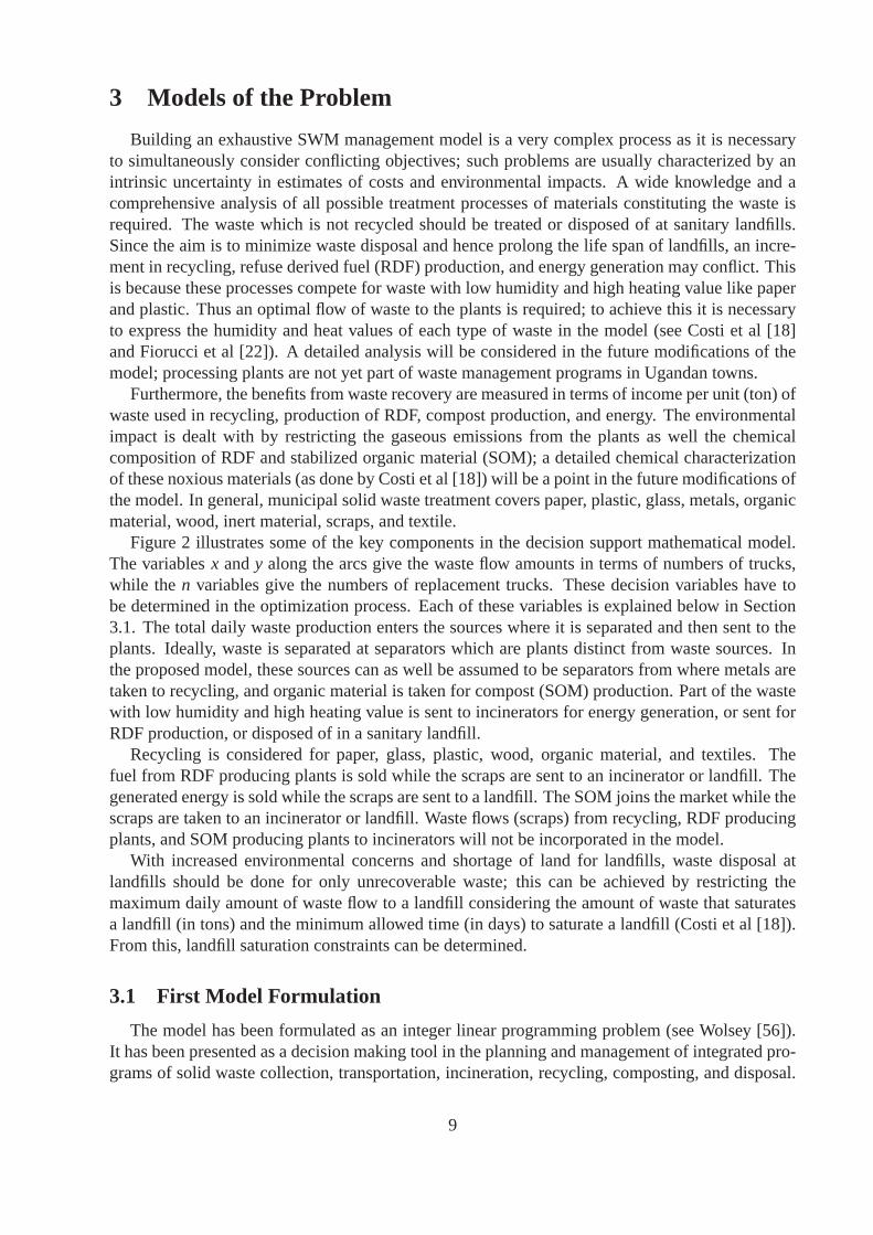
Figure 2 illustrates some of the key components in the decision support mathematical model.The variablesx andy along the arcs give the waste flow amounts in terms of numbers of trucks,while then variables give the numbers of replacement trucks. These decision variables have tobe determined in the optimization process. Each of these variables is explained below in Section3.1. The total daily waste production enters the sources where it is separated and then sent to theplants. Ideally, waste is separated at separators which areplants distinct from waste sources. Inthe proposed model, these sources can as well be assumed to beseparators from where metals aretaken to recycling, and organic material is taken for compost (SOM) production. Part of the wastewith low humidity and high heating value is sent to incinerators for energy generation, or sent forRDF production, or disposed of in a sanitary landfill.

Recycling is considered for paper, glass, plastic, wood, organic material, and textiles. Thefuel from RDF producing plants is sold while the scraps are sent to an incinerator or landfill. Thegenerated energy is sold while the scraps are sent to a landfill. The SOM joins the market while thescraps are taken to an incinerator or landfill. Waste flows (scraps) from recycling, RDF producingplants, and SOM producing plants to incinerators will not beincorporated in the model.

With increased environmental concerns and shortage of landfor landfills, waste disposal atlandfills should be done for only unrecoverable waste; this can be achieved by restricting themaximum daily amount of waste flow to a landfill considering the amount of waste that saturatesa landfill (in tons) and the minimum allowed time (in days) to saturate a landfill (Costi et al [18]).From this, landfill saturation constraints can be determined.

3.1 First Model Formulation

The model has been formulated as an integer linear programming problem (see Wolsey [56]).It has been presented as a decision making tool in the planning and management of integrated pro-grams of solid waste collection, transportation, incineration, recycling, composting, and disposal.

9

#"

!

#"

!

#"

!

?

?

6

6

?

6

?

?

?

-

-

?

-6

-

-

sourcei

RDF plantm

market

energy

SOM planth

incineratorj

recycling plants

truck depotr

landfillkxl

ikg

xlisg

nlri

nlrh

nlrm

nlrk

nlrs

nlr j

xli jg

ylmkg

xlihg

ylhkg

yljkg

ylskg

xlimg

Figure 2: A detailed representation of key components in a decision support mathematical model.

10

The waste collection component has not been considered but several treatment plants and facilitieshave been included within the proposed model: trucks for thetransportation of waste; replacementtrucks and their depots; incinerators with energy recovery; sanitary landfills; plants for recycling,production of RDF, and treatment of organic material.

The objective function consists of total cost owing to investment and management costs, trans-portation costs, operational costs from the use of replacement trucks, benefits from energy genera-tion, RDF production, compost, and recycling. The constraints include waste flow constraints dueto the movement of waste among sources and plants and landfills as well as capacity, site selec-tion, facility availability, environmental, and landfill saturation constraints. Constraints owing tothe utilization of replacement trucks have also been included.

It is assumed that a waste manager in a municipality has a database of all the parameters on thecomputer well written in AMPL language as well as the model where all this data is supposed tobe fed for a solution whenever required. There should also bean AMPL compatible solver likeCPLEX on the computer. The advantage of having a database in AMPL is that it is easy to modifyaccording to the changes in the parameters, and because modification of data does not require anexpert in programming but one who can enter/change data in a proper way. The first use of themodel determines all costs including investment costs; thesubsequent uses, depending on whethersignificant changes have been observed in some of the key parameters, determine transport andoperational costs, etc. The location of facilities will have been done in the first application ofthe model. Decisions are taken whenever required by considering the results. In the day to dayapplication of the models, it may be more orderly and cheaperto hire replacement trucks insteadof buying them.

The model has been built upon the following assumptions:

1. “Waste source” are located at the centres of waste generating areas.

2. Waste separation is done at the waste source locations (collection points). In other words,we can identify these sources with separators in this case. In practice sources and separatorsare distinct.

3. Waste handling operations proposed in the model are to be executed daily.

The ambiguity of the first assumption is that “radii” of wastegenerating areas are not specified;the point is that if the areas are almost “circular” and the “radii” are “small”, then the wastecollection points at the centres are uniformly accessible from within the areas. The drawback isthat the shapes and sizes of the waste areas can be very erratic so that the accessibility of the wastecollection points at the centres may not be uniform from within the entire area; some of the wastemay then not reach these collection points.

The advantage of the second assumption is that no money is then spent on establishing sepa-rators; it is however largely dependent on the cooperation of waste generators, the volume/weightand nature of waste generated. The most realistic option maybe to have separators in the model,to which some of the waste is channelled for separation before transportation to recycling, SOMand RDF producing, and incinerating plants.

The third assumption is advantageous for daily heavy waste producing waste sources; the draw-back is that waste sources that require weekly or monthly collections are not directly catered forin the model. Probably in the daily utilization of the model,some of the parameters (like costs) ofsuch waste sources can be considered as “zeroes” until the days when they require collections.

11

Indices

i = 1, 2, . . . , I: location of waste sources (collection points).

j = 1, 2, . . . , J: location of incinerators.

k = 1, 2, . . . ,K: location of sanitary landfills.

r = 1, 2, . . . ,R: location of replacement trucks depots.

m = 1, 2, . . . ,M: location of refuse derived fuel (RDF) plants.

h = 1, 2, . . . ,H: location of composting (stabilized organic material, SOM) plants.

s = 1, 2, . . . , S : location of recycling plants.

l = 1, 2, . . . , L: truck type.

g = 1, 2, . . . ,G: waste type.

Variables

Xli jg, Xl

img, Xlihg, Xl

isg, Xlikg: respectively total number of trips made by trucks of typel used every-

day to carry waste of typeg from waste sourcei to an incinerator atj, an RDF plant atm, an SOMplant ath, a recycling plant ats, and a landfill atk.

xli jg, xl

img, xlihg, xl

isg, xlikg: respectively number of trucks of typel used everyday to carry waste of

typeg from waste sourcei to an incinerator atj, an RDF plant atm, an SOM plant ath, a recyclingplant ats, and a landfill atk.

Y ljkg, Y l

mkg, Y lhkg, Y l

skg: respectively total number of trips made by trucks of typel used everydayto carry waste of typeg from an incinerator atj, an RDF plant atm, an SOM plant ath, and arecycling plant ats to a landfill atk.

yljkg, yl

mkg, ylhkg, yl

skg: respectively number of trucks of typel used everyday to carry waste of typeg from an incinerator atj, an RDF plant atm, an SOM plant ath, and a recycling plant ats to alandfill at k.

nlr j, nl

rm, nlrh, nl

rs, nlrk, nl

ri: respectively number of trucks of typel used everyday from a replace-ment trucks depot atr to an incinerator atj, an RDF plant atm, an SOM plant ath, a recyclingplant ats, a landfill atk, and a waste source ati.

z j, zm, zh, zs, zk, zr: 0-1 variables indicating respectively, the presence of anincinerator atj, anRDF plant atm, an SOM plant ath, a recycling plant ats, a landfill atk, and a replacement trucksdepot atr.

w j, wm, wh, ws, tk: amount of waste transported everyday respectively, to an incinerator atj, anRDF plant atm, an SOM plant ath, a recycling plant ats, and a sanitary landfill atk.

Tl : The number of trucks of typel used everyday.

T : The total number of trucks (excluding replacement trucks)used everyday.

(RT )l : The number of replacement trucks of typel required everyday.

12

Input Data /Parameters

ali j, al

im, alih, al

is, alik: expected number of trips a truck of typel can make respectively, per day

between waste source ati and an incinerator atj, an RDF plant atm, an SOM plant ath, a recyclingplant ats, and a landfill atk.

bljk, bl

mk, blhk, bl

sk: expected number of trips a truck of typel can make respectively, per day betweenan incinerator atj, an RDF plant atm, an SOM plant ath, a recycling plant ats, and a landfill atk.

αl: capacity (in tonnes) of a truck of typel.

pl: probability that a truck of typel breaks down in a day.

Ωe: upper limit for noxious substancee; e = 1, 2, . . . , E.

elrk, el

r j, elrm, el

rh, elrs, el

ri: respectively the cost of moving a truck of typel from a replacementtrucks depot atr to a landfill atk, an incinerator atj, an RDF plant atm, an SOM plant ath, arecycling plant ats, and a waste source ati.

cli j, cl

im, clih, cl

is, clik: respectively transportation cost per unit of waste carried by a truck of typel

from a waste source ati to an incinerator atj, an RDF plant atm, an SOM plant ath, a recyclingplant ats, and a landfill atk.

dljk, dl

mk, dlhk, dl

sk: respectively transportation cost per unit of waste carried by a truck of typelfrom an incinerator atj, an RDF plant atm, an SOM plant ath, and a recycling plant ats to alandfill at k.

c j, cm, ch, cs: revenue respectively, per unit of waste at an incinerator at j, an RDF plant atm, anSOM plant ath, and a recycling plant ats.

fl: the cost of buying a new truck of typel, l = 1 . . . , L.

di: amount of waste at sourcei.

ρ j, ρm, ρh, ρs: fraction (%) of unrecovered waste respectively, at an incinerator atj, an RDF plantat m, an SOM plant ath, and a recycling plant ats that requires disposal to a landfill.

Q j, Qm, Qh, Qs, Qk, Qr: capacity per day respectively, for an incinerator atj, an RDF plant atm,an SOM plant ath, a recycling plant ats, a landfill atk, and a replacement trucks depot atr.

δ j, δm, δh, δs, δk, δr: respectively fixed cost incurred in opening an incineratorat j, an RDF plantat m, an SOM plant ath, a recycling plant ats, a landfill atk, and a replacement trucks depot atr.

γ j, γm, γh, γs, γk: respectively variable cost incurred in handling a unit of waste at an incineratorat j, an RDF plant atm, an SOM plant ath, a recycling plant ats, and a landfill atk.

µej, µ

em, µ

eh, µ

es, µ

ek: respectively amount of noxious materiale generated (per unit of waste) at an

incinerator atj, an RDF plant atm, an SOM plant ath, a recycling plant ats, and a sanitary landfillat k; e = 1, 2, . . . , E.

Objective Function

The objective function represents the overall daily waste management costs; the first compo-nent gives the investment and waste handling expenses as well as transportation costs, the secondcomponent gives expenses owing to the use of replacement trucks, and the third component theincome from waste products like refuse derived fuel and energy.

The first componentF1 refers to the overall costs; the first part deals with the investment and

13

management expenses while the second is concerned with the transportation costs. The two partsare separated by two sets of square brackets in (1). In this function we have the fixed cost pa-rametersδ, and the variable cost parametersγ. The variablesX andY have been defined at thebeginning of Section 3.1.

F1(z,w, X,Y) = [∑

j

(δ jz j + γ jw j) +∑

m

(δmzm + γmwm)

+∑

h

(δhzh + γhwh) +∑

s

(δszs + γsws) +∑

k

(δkzk + γktk)]

+ [∑

gli j

cli jαlX

li jg +

∑

glim

climαlX

limg +

∑

glih

clihαlX

lihg +

∑

glis

clisαlX

lisg

+∑

glik

clikαlX

likg +

∑

gl jk

dljkαlY

ljkg +

∑

glmk

dlmkαlY

lmkg +

∑

glhk

dlhkαlY

lhkg

+∑

glsk

dlskαlY

lskg] (1)

ComponentF2 concerns the total costs owing to the presence of replacement trucks (or standbytrucks). ComponentF3 gives the total cost for buying all trucks required in the daily managementof waste. ComponentB gives the benefits at the plants owing to the production of electric energy,compost, refuse derived fuel, and recycled material.

F2(n, z) =∑

rkl

elrkn

lrk +

∑

r jl

elr jn

lr j +

∑

rml

elrmnl

rm +∑

rhl

elrhnl

rh

+∑

rsl

elrsn

lrs +

∑

ril

elrin

lri +

∑

r

δrzr (2)

F3(x, y, n) =∑

l

fl(Tl + (RT )l) (3)

B(w) =∑

j

c j(1 − ρ j)w j +∑

m

cm(1 − ρm)wm +∑

h

ch(1 − ρh)wh

+∑

s

cs(1 − ρs)ws (4)

So the objective functionF, to be minimized, is

F = F1 + F2 + F3 − B (5)

14

Constraints

In general, the constraints include those linking waste flowamong sources and plants and land-fills, as well as capacity, site selection, facility availability, environmental, and landfill saturationconstraints. The desire in constraint (6) is to clear all thewaste generated at the source (collectionpoint) i. So the total waste moved from each waste collection pointi should at least be equal to theamount of waste found at that point.

∑

gl j

αlXli jg +

∑

glm

αlXlimg +

∑

glh

αlXlihg +

∑

glh

αlXlisg +

∑

glk

αlXlikg ≥ di, i = 1, . . . , I (6)

In constraints (7)-(10), it is meant that the waste generated by a processing plant is disposed ofin a landfill (or tip). Thus the amount of waste carried away from every plant to a landfill, shouldat least be equal to the amount of waste found at that plant. Itis important to note that the weightof waste carried by a truck in a single trip (from a given source) is at most equal to its capacity,depending on the waste type and its amount; so the inequalities in (6) and (7)-(10) make sense.

ρ jw j ≤∑

gkl

αlYljkg, j = 1, . . . , J (7)

ρmwm ≤∑

gkl

αlYlmkg, m = 1, . . . ,M (8)

ρhwh ≤∑

gkl

αlYlhkg, h = 1, . . . ,H (9)

ρsws ≤∑

gkl

αlYlskg, s = 1, . . . , S (10)

Constraint (11) means that the amount of noxious material must not exceed National Environ-mental Management Authority or international levels,Ωe.

∑

j

µej(1 − ρ j)w j +

∑

m

µem(1 − ρm)wm +

∑

h

µeh(1 − ρh)wh

+∑

s

µes(1 − ρs)ws +

∑

k

µektk ≤ Ωe, e = 1, . . . , E (11)

In constraints (12)-(15) the maximum capacities for the processing plants are accounted for.These constraints mean that the amount of waste taken to these plants should not exceed the plantcapacities. In constraint (16) the same thing is done for sanitary landfills.

w j ≤ Q jz j, j = 1, . . . , J (12)

wm ≤ Qmzm, m = 1, . . . ,M (13)

wh ≤ Qhzh, h = 1, . . . ,H (14)

ws ≤ Qszs, s = 1, . . . , S (15)

tk ≤ Qkzk, k = 1, 2, . . . ,K (16)

15

Constraint (17), means that the total number of replacement trucks of typel cannot be less thanthe expected number of daily truck breakdowns of the typel. With constraint (18), we ensure thatthere is at least one depot for the replacement trucks. In constraint (19) we codify that the numberof trucks in a depot cannot exceed its capacity. Constraint (20) means that the total number ofreplacement trucks is not too big compared to the total number of trucks used per day.

∑

rk

nlrk +

∑

r j

nlr j +

∑

rm

nlrm +

∑

rh

nlrh +

∑

rs

nlrs +

∑

ri

nlri ≥ plTl,

l = 1, . . . , L (17)

R∑

r=1

zr ≥ 1 (18)

∑

lk

nlrk +

∑

l j

nlr j +

∑

lm

nlrm +

∑

lh

nlrh +

∑

ls

nlrs +

∑

lri

nlri ≤ Qrzr,

r = 1, . . . ,R (19)∑

r

Qrzr ≤ T (20)

Constraints (21)-(29) mean that once the flow to either plant or sanitary landfill is positive, thatplant or landfill must actually exist. The variablesX andY have been defined at the beginningof Section 3.1 and under definitions (51)-(59). We note here,as an example, that the expressioni, ( j) = 1, . . . , I, (J) means thati ranges from 1 up toI and j ranges from 1 up toJ.

αlXli jg ≤ Q jz j, l = 1, . . . , L, i, ( j) = 1, . . . , I, (J), g = 1, . . . , G (21)

αlXlimg ≤ Qmzm, l = 1, . . . , L, i, (m) = 1, . . . , I, (M), g = 1, . . . ,G (22)

αlXlihg ≤ Qhzh, l = 1, . . . , L, i, (h) = 1, . . . , I, (H), g = 1, . . . , G (23)

αlXlisg ≤ Qszs, l = 1, . . . , L, i, (s) = 1, . . . , I, (S ), g = 1, . . . , G (24)

αlXlikg ≤ Qkzk, l = 1, . . . , L, i, (k) = 1, . . . , I, (K), g = 1, . . . , G (25)

αlYljkg ≤ Qkzk, l = 1, . . . , L, j, (k) = 1, . . . , J, (K), g = 1, . . . , G (26)

αlYlmkg ≤ Qkzk, l = 1, . . . , L, m, (k) = 1, . . . , M, (K), g = 1, . . . , G (27)

αlYlhkg ≤ Qkzk, l = 1, . . . , L, h, (k) = 1, . . . , H, (K), g = 1, . . . , G (28)

αlYlskg ≤ Qkzk, l = 1, . . . , L, s, (k) = 1, . . . , S , (K), g = 1, . . . , G (29)

Variable Conditions

The variables in constraints (30)-(38) are defined as non-negative integers. These give the num-ber of trucks used between two nodes in the model per day, excluding replacement trucks.

xli jg, integer ≥ 0, i, ( j) = 1, . . . , I, (J), l = 1, . . . , L, g = 1, . . . , G (30)

16

xlimg, integer ≥ 0, i, (m) = 1, . . . , I, (M), l = 1, . . . , L, g = 1, . . . , G (31)

xlihg, integer ≥ 0, i, (h) = 1, . . . , I, (H), l = 1, . . . , L, g = 1, . . . , G (32)

xlisg, integer ≥ 0, i, (s) = 1, . . . , I, (S ), l = 1, . . . , L, g = 1, . . . , G (33)

xlikg, integer ≥ 0, i, (k) = 1, . . . , I, (K), l = 1, . . . , L, g = 1, . . . , G (34)

yljkg, integer ≥ 0, j, (k) = 1, . . . , J, (K), l = 1, . . . , L, g = 1, . . . , G (35)

ylmkg, integer ≥ 0, m, (k) = 1, . . . ,M, (K), l = 1, . . . , L, g = 1, . . . , G (36)

ylhkg, integer ≥ 0, h, (k) = 1, . . . ,H, (K), l = 1, . . . , L, g = 1, . . . , G (37)

ylskg, integer ≥ 0, s, (k) = 1, . . . , S , (K), l = 1, . . . , L, g = 1, . . . , G (38)

The variables in constraints (39)-(44) are defined as non-negative integers. These give the num-ber of replacement trucks required everyday in the waste management program. We note that thebreakdown of a truck can occur anywhere in the road network followed by the trucks. For purposesof locating the truck depots, it is assumed that these breakdowns occur at either a waste collectionpoint or at a plant or at a landfill.

nlrk, integer ≥ 0, r, (k) = 1, . . . ,R, (K), l = 1, . . . , L (39)

nlr j, integer ≥ 0, r, ( j) = 1, . . . ,R, (J), l = 1, . . . , L (40)

nlrm, integer ≥ 0, r, (m) = 1, . . . ,R, (M), l = 1, . . . , L (41)

nlrh, integer ≥ 0, r, (h) = 1, . . . ,R, (H), l = 1, . . . , L (42)

nlrs, integer ≥ 0, r, (s) = 1, . . . ,R, (S ), l = 1, . . . , L (43)

nlri, integer ≥ 0, r, (i) = 1, . . . ,R, (I), l = 1, . . . , L (44)

The variables in (45)-(50) are defined as boolean. These are used to determine the existence ofeither a plant or a landfill.

z j ∈ 0, 1, j = 1, . . . , J (45)

zm ∈ 0, 1, m = 1, . . . ,M (46)

zh ∈ 0, 1, h = 1, . . . ,H (47)

zs ∈ 0, 1, s = 1, . . . , S (48)

zk ∈ 0, 1, k = 1, . . . ,K (49)

zr ∈ 0, 1, r = 1, . . . ,R (50)

Definitions

In equations (51)-(59) the expected number of trips made perday by the trucks of typel fromwaste sources to plants, waste sources to landfills, and plants to landfills are given.

Xli jg = al

i j xli jg, l = 1, . . . , L, i, ( j) = 1, . . . , I, (J), g = 1, . . . , G (51)

Xlimg = al

im xlimg, l = 1, . . . , L, i, (m) = 1, . . . , I, (M), g = 1, . . . , G (52)

17

Xlihg = al

ih xlihg, l = 1, . . . , L, i, (h) = 1, . . . , I, (H), g = 1, . . . , G (53)

Xlisg = al

is xlisg, l = 1, . . . , L, i, (s) = 1, . . . , I, (S ), g = 1, . . . , G (54)

Xlikg = al

ikxlikg, l = 1, . . . , L, i, (k) = 1, . . . , I, (K), g = 1, . . . , G (55)

Y ljkg = bl

jkyljkg, l = 1, . . . , L, j, (k) = 1, . . . , J, (K), g = 1, . . . , G (56)

Y lmkg = bl

mkylmkg, l = 1, . . . , L, m, (k) = 1, . . . , M, (K), g = 1, . . . , G (57)

Y lhkg = bl

hkylhkg, l = 1, . . . , L, h, (k) = 1, . . . , H, (K), g = 1, . . . , G (58)

Y lskg = bl

skylskg, l = 1, . . . , L, s, (k) = 1, . . . , S , (K), g = 1, . . . , G (59)

Definitions (60)-(63), also mentioned at the beginning of Section 3.1, indicate the amount ofwaste transported to processing plants while definition (64) gives the amount of waste from allwaste sources to a landfillk. Similarly, definition (65) indicates the amount of waste disposed ofin a sanitary landfillk everyday. Equation (66) gives the total amount of waste collected from allwaste sources per day; this excludes waste generated by the plants. In equation (67) we give thetotal number of trucks of typel used per day in the model and, in definition (68) the total numberof trucks required per day for the transportation, treatment, and disposal of waste is determined. Indefinition (69) the number of replacement trucks of typel in each depot is given, and in equation(70) the total number of replacement trucks in all depots is determined. It is assumed that thetrucks are fully loaded as they leave the waste collection points.

w j =∑

gli

αlXli jg, j = 1, . . . , J (60)

wm =∑

gli

αlXlimg, m = 1, . . . ,M (61)

wh =∑

gli

αlXlihg, h = 1, . . . ,H (62)

ws =∑

gli

αlXlisg, s = 1, . . . , S (63)

wk =∑

gli

αlXlikg, k = 1, . . . ,K (64)

tk = wk +∑

gl j

αlYljkg +

∑

glm

αlYlmkg +

∑

glh

αlYlhkg +

∑

gls

αlYlskg, k = 1, . . . ,K (65)

W =∑

j

w j +∑

m

wm +∑

h

wh +∑

s

ws +∑

k

wk (66)

Tl =∑

gi j

xli jg +

∑

gim

xlimg +

∑

gih

xlihg +

∑

gis

xlisg +

∑

gik

xlikg +

∑

g jk

yljkg

+∑

gmk

ylmkg +

∑

ghk

ylhkg +

∑

gsk

ylskg, l = 1, . . . , L (67)

18

T =∑

l

Tl (68)

(RT )l =∑

rk

nlrk +

∑

r j

nlr j +

∑

rm

nlrm +

∑

rh

nlrh +

∑

rs

nlrs +

∑

ri

nlri, l = 1, . . . , L (69)

RT =∑

l

(RT )l (70)

3.2 Analysis of the First Model

As mentioned at the beginning of Section 3.1, the model has been formulated as an integer linearprogramming problem (Wolsey [56]). The constraints include waste flow constraints for sourcesand plants and landfills, capacity, site selection, facility availability, environmental, and landfillsaturation constraints. Truck flow constraints for replacement trucks from depots to landfills, wastesources, and processing plants have also been included.

We have a single objective function that covers the overall economic cost in the model. Accord-ing to Costi et al [18], the definition of a decision model concerning the design of an urban solidwaste management system would require the use of multi-objective decision concepts and tech-niques. Our model, like that of Costi et al [18], is particularly oriented to real-world applications;the multi-objective nature is taken into account by considering a single optimization objective com-prising the overall economic cost, and transforming all other objectives (on pollution containment,impact minimization, etc) into constraints. Through theseconstraints it becomes easier to dealwith regulations that specify bounds on the release of pollutants and other negative effects on theenvironment.

It is a deterministic model with integral decision variables; this was motivated by the desire ofnot only measuring waste quantities handled but also count the number of trucks of every typebeing used in the model. For instance in equation (67) we find the number of trucks of each typewhile in equation (68) we find the total number of trucks that operate daily in the model. Throughequation (69) we determine the number of replacement trucksof each type that we may need dailywhile through equation (70) the total number of replacementtrucks needed in the model per day iscomputed.

Since it is linear, it can be solved to optimality by several modelling/solver packages on themarket like AMPL/CPLEX, LINGO/LINDO, GAMS/CPLEX, and MPL/CPLEX. The package,AMPL/CPLEX, we intend to use is briefly described in Section 5. The formulation of this modellies within the field of operations research that has been usefully applied to a wide variety ofenvironmental problem areas (see ReVelle [53]).

The benefits from waste in the third componentB of the objective function are measured interms of economic gain per unit of waste. In actual terms it should be measured in terms of salesper litre of RDF produced, unit of SOM produced, unit of energyproduced, unit item producedfrom recycling. To simplify the mathematics in the model, this precision was indirectly looked atin terms of economic gain per unit of waste. Another point is that we do not yet have processingplants in Uganda although it is under consideration. This explains why we do not have regulatoryand technical constraints (see Costi et al [18] and Fiorucci et al [22]) in the model. We alsohave only one landfill. We have included economic gains from recycling in the benefits function;according to Costi et al [18] and Fiorucci et al [22], recycling in reality produces net cost. It ishowever encouraged because of environmental concerns and optimal use of limited resources.

19

The fractionsρ of unrecovered waste at the plants, and the amountsµ of noxious substancesgenerated at the plants and landfills are assumed to be independent of the type of waste in bothmodels. It is more realistic to consider dependence on the type of waste in order to formulate moreprecise environmental constraints, etc.

It is worth mentioning here that the current waste management trend in Uganda indicates thatwe are likely to have private companies that only collect waste, companies that only treat waste,and possibly companies that only manage sanitary landfills.The future waste models are likely tohave these three scenarios of waste management where regulatory and technical constraints will beof major interest to companies running processing plants and landfills. Probably these companieswill later merge to form integrated waste management programs. The proposed model is a goodstarting point upon which future variations can be built.

We shall also not go into a detailed description of environmental impacts as done by Costiet al [18], with specific attention paid to incineration emissions and RDF chemical composition.They consider pollutant content in the RDF, in the SOM, and incineration emissions. We measurepollutant content through unit waste handled at the plants;this may not be precise but a goodillustration of how environmental impact can be considered. The consideration of the regulatory,technical, and a detailed description of environmental constraints may be done without affectingthe linearity of the models. The biggest problem so far in Uganda with regard to waste pollutionsprings from the fact that much of the waste generated in Ugandan towns is not actually collected.

We have mentioned landfill saturation constraints (16) in the model in Section 3.1; the dailycapacityQk imposed on the landfillk will be determined according to our desire of keeping thatlandfill active for a determined minimum number of years. Thequality of the technology in placeis very crucial here. That is to say, we shall determine the total amount of waste that saturates thatlandfill and divide it with the number of days that constitutethe determined minimum number ofyears we want the landfill to remain active.

The environmental constraints (11) have been presented in avery elementary form in order tokeep the mathematics simple; a detailed and precise description has been done by Costi et al [18].A detailed description also requires a deep knowledge and analysis of all the processes involved.These constraints regulate the pollutant emissions at the plants as well as the toxic composition ofthe RDF and the SOM produced.

With constraint (18) we can, in theory, ensure that (it is presumed that these probabilities areknown by the waste managers) there is at least one depot for replacement trucks. This may beridiculous in practice in case of no breakdowns (especiallyif the trucks are new)! An alternative tobuying replacement trucks may be hiring them in case of breakdowns. This may be more practicaland can also keep the daily operational costs down. However,this constraint is not unreasonablesince specialized trucks may be used in the management programs, and consequently not easilyobtainable through hiring.

3.3 The Second Model of the Problem

In this section, a variant of the integer linear model described in Section 3.1 is presented with thehope of getting better total cost estimates and waste amountmeasurements. Continuous variablesu’s andv’s have been introduced; they respectively measure the amount of waste collected everydayfrom waste sources to plants and from plants to landfills. A mixed integer linear program is thusobtained (see Wolsey [56]); the description of the new variablesu andv now follows.

1. uli jg, ul

img, ulihg, ul

isg, ulikg: respectively amount of waste (in tons) of typeg collected everyday

20

by trucks of typel from a waste sourcei to an incinerator atj, an RDF plant atm, an SOMplant ath, a recycling plant ats, and a landfill atk.

2. vljkg, vl

mkg, vlhkg, vl

skg: respectively amount of waste (in tons) of typeg collected everydayby trucks of typel from an incinerator atj, an RDF plant atm, an SOM plant ath, and arecycling plant ats to a landfill atk.

The description of the rest of the variables and parameters in the model, remains the same as inSection 3.1.

Let it be noted that the emergence of the mixed integer linearmodel nowhere undermines theimportance of the integer linear model; the choice between the two models from the practicalpoint of view depends on the user and the technology used. Oneuser may prefer to measure thetransportation costs in terms of costs per trip made from thewaste source, in which case the firstmodel is more appropriate. In this case we replace the coefficients of the variablesX andY inthe objective function with the total cost per trip from the waste collection point. At the sametime, instead of measuring the amount of waste using the number of trucks used multiplied bytheir capacities, continuous variables can be introduced to measure directly the amount of wastethat goes to the plants and landfills. The integer linear problem is then transformed into a mixedinteger problem that gives better total cost estimates and more precise waste amount measurements.For instance, at the moment the first model is more relevant tothe Ugandan situation, where thetechnology to measure waste as it is carried away from the waste sources is not available. Anotheruser may prefer to measure the transportation costs in termsof costs per unit mass of waste pickedfrom the waste source, in which case the second model is more appropriate.

Objective Function

The objective function, like in Section 3.1, represents theoverall daily waste management costs;the first component gives the investment and waste handling expenses as well as transportationcosts, the second component gives expenses owing to the use of replacement trucks, and the thirdcomponent the income from waste products like refuse derived fuel and energy.

The first componentF1 refers to the overall costs; the first part deals with the investment andmanagement expenses while the second is concerned with the transportation costs. The two partsare separated by two sets of square brackets in (71). In this function we have the fixed cost parame-tersδ, and the variable cost parametersγ. The variablesu andv have been defined at the beginningof this section.

F1(z,w, u, v) = [∑

j

(δ jz j + γ jw j) +∑

m

(δmzm + γmwm)

+∑

h

(δhzh + γhwh) +∑

s

(δszs + γsws) +∑

k

(δkzk + γktk)]

+ [∑

gli j

cli ju

li jg +

∑

glim

climul

img +∑

glih

clihul

ihg +∑

glis

clisu

lisg +

∑

glik

cliku

likg

+∑

gl jk

dljkv

ljkg +

∑

glmk

dlmkv

lmkg +

∑

glhk

dlhkv

lhkg +

∑

glsk

dlskv

lskg] (71)

21

ComponentF2 concerns the total costs owing to the presence of replacement trucks (or standbytrucks). ComponentF3 gives the total cost for buying all trucks required in the daily managementof waste. ComponentB gives the benefits at the plants owing to the production of electric energy,compost, refuse derived fuel, and recycled material.

F2(n, z) =∑

rkl

elrkn

lrk +

∑

r jl

elr jn

lr j +

∑

rml

elrmnl

rm +∑

rhl

elrhnl

rh

+∑

rsl

elrsn

lrs +

∑

ril

elrin

lri +

∑

r

δrzr (72)

F3(x, y, n) =∑

l

fl(Tl + (RT )l) (73)

B(w) =∑

j

c j(1 − ρ j)w j +∑

m

cm(1 − ρm)wm +∑

h

ch(1 − ρh)wh

+∑

s

cs(1 − ρs)ws (74)

So we then obtain the objective functionF, to be minimized, defined as

F = F1 + F2 + F3 − B (75)

Constraints

In general, the constraints are the capacity, site selection, facility availability, environmental,and landfill saturation constraints. In constraint (76) we make sure that the total waste moved fromeach waste collection pointi is at least be equal to the amount of waste found at that point.

∑

gl j

uli jg +

∑

glm

ulimg +

∑

glh

ulihg +

∑

glh

ulisg +

∑

glk

ulikg ≥ di, i = 1, . . . , I (76)

In constraints (77)-(80), we guarantee that the amount of waste carried away from every plantto a landfill, is at least be equal to the amount of waste found at that plant.

ρ jw j ≤∑

gkl

vljkg, j = 1, . . . , J (77)

ρmwm ≤∑

gkl

vlmkg, m = 1, . . . ,M (78)

ρhwh ≤∑

gkl

vlhkg, h = 1, . . . ,H (79)

ρsws ≤∑

gkl

vlskg, s = 1, . . . , S (80)

22

In constraint (81) the amount of noxious material must not exceed National EnvironmentalManagement Authority or international levels,Ωe.

∑

j

µej(1 − ρ j)w j +

∑

m

µem(1 − ρm)wm +

∑

h

µeh(1 − ρh)wh

+∑

s

µes(1 − ρs)ws +

∑

k

µektk ≤ Ωe, e = 1, . . . , E (81)

In constraints (82)-(85) the maximum capacities for the processing plants are determined. Theseconstraints mean that the amount of waste taken to these plants should not exceed the plant capac-ities. In constraint (86) the same is done for sanitary landfills.

w j ≤ Q jz j, j = 1, . . . , J (82)

wm ≤ Qmzm, m = 1, . . . ,M (83)

wh ≤ Qhzh, h = 1, . . . ,H (84)

ws ≤ Qszs, s = 1, . . . , S (85)

tk ≤ Qkzk, k = 1, 2, . . . ,K (86)

In constraint (87), the total number of replacement trucks of type l cannot be less than theexpected number of daily truck breakdowns of the typel. With constraint (88), we ensure thatthere is at least one depot for the replacement trucks. In constraint (89) we codify that the numberof trucks in a depot cannot exceed its capacity. Constraint (90) guarantees that the total number ofreplacement trucks is not too big compared to the total number of trucks used per day.

∑

rk

nlrk +

∑

r j

nlr j +

∑

rm

nlrm +

∑

rh

nlrh +

∑

rs

nlrs +

∑

ri

nlri ≥ plTl,

l = 1, . . . , L (87)

R∑

r=1

zr ≥ 1 (88)

∑

lk

nlrk +

∑

l j

nlr j +

∑

lm

nlrm +

∑

lh

nlrh +

∑

ls

nlrs +

∑

lri

nlri ≤ Qrzr,

r = 1, . . . ,R (89)∑

r

Qrzr ≤ T (90)

Constraints (91)-(99) mean that once the flow to either plant or sanitary landfill is positive, thatplant or landfill must actually exist.

uli jg ≤ Q jz j, l = 1, . . . , L, i, ( j) = 1, . . . , I, (J), g = 1, . . . , G (91)

ulimg ≤ Qmzm, l = 1, . . . , L, i, (m) = 1, . . . , I, (M), g = 1, . . . ,G (92)

ulihg ≤ Qhzh, l = 1, . . . , L, i, (h) = 1, . . . , I, (H), g = 1, . . . , G (93)

23

ulisg ≤ Qszs, l = 1, . . . , L, i, (s) = 1, . . . , I, (S ), g = 1, . . . , G (94)

ulikg ≤ Qkzk, l = 1, . . . , L, i, (k) = 1, . . . , I, (K), g = 1, . . . , G (95)

vljkg ≤ Qkzk, l = 1, . . . , L, j, (k) = 1, . . . , J, (K), g = 1, . . . , G (96)

vlmkg ≤ Qkzk, l = 1, . . . , L, m, (k) = 1, . . . , M, (K), g = 1, . . . , G (97)

vlhkg ≤ Qkzk, l = 1, . . . , L, h, (k) = 1, . . . , H, (K), g = 1, . . . , G (98)

vlskg ≤ Qkzk, l = 1, . . . , L, s, (k) = 1, . . . , S , (K), g = 1, . . . , G (99)

The constraints in (100)-(108) relate the amount of waste collected from any waste source perday with the number of trucks used to collect that waste. Theymean that the waste carried by thesetrucks from the waste collection points cannot exceed the amount of waste they can carry whenfully loaded.

uli jg ≤ αla

li j x

li jg, l = 1, . . . , L, i, ( j) = 1, . . . , I, (J), g = 1, . . . , G (100)

ulimg ≤ αla

lim xl

img, l = 1, . . . , L, i, (m) = 1, . . . , I, (M), g = 1, . . . , G (101)

ulihg ≤ αla

lih xl

ihg, l = 1, . . . , L, i, (h) = 1, . . . , I, (H), g = 1, . . . , G (102)

ulisg ≤ αla

lis x

lisg, l = 1, . . . , L, i, (s) = 1, . . . , I, (S ), g = 1, . . . , G (103)

ulikg ≤ αla

likxl

ikg, l = 1, . . . , L, i, (k) = 1, . . . , I, (K), g = 1, . . . , G (104)

vljkg ≤ αlb

ljky

ljkg, l = 1, . . . , L, j, (k) = 1, . . . , J, (K), g = 1, . . . , G (105)

vlmkg ≤ αlb

lmky

lmkg, l = 1, . . . , L, m, (k) = 1, . . . , M, (K), g = 1, . . . , G (106)

vlhkg ≤ αlb

lhky

lhkg, l = 1, . . . , L, h, (k) = 1, . . . , H, (K), g = 1, . . . , G (107)

vlskg ≤ αlb

lsky

lskg, l = 1, . . . , L, s, (k) = 1, . . . , S , (K), g = 1, . . . , G (108)

Constraints (109)-(117) can be referred to as waste flow fixingconstraints. The reason is thatwhen there are benefits at some node there is a tendency to moveas much waste as possible tothat node as long as there is space on the truck. In such a case,what is “carried” on the truck, thatincludes false waste, may go beyond the amount at a waste source; this is undesirable because theinterest is in the precise amount of waste picked from the source.

uli jg ≤ di, l = 1, . . . , L, i, ( j) = 1, . . . , I, (J), g = 1, . . . , G (109)

ulimg ≤ di, l = 1, . . . , L, i, (m) = 1, . . . , I, (M), g = 1, . . . ,G (110)

ulihg ≤ di, l = 1, . . . , L, i, (h) = 1, . . . , I, (H), g = 1, . . . , G (111)

ulisg ≤ di, l = 1, . . . , L, i, (s) = 1, . . . , I, (S ), g = 1, . . . , G (112)

ulikg ≤ di, l = 1, . . . , L, i, (k) = 1, . . . , I, (K), g = 1, . . . , G (113)

vljkg ≤ ρ jw j, l = 1, . . . , L, j, (k) = 1, . . . , J, (K), g = 1, . . . , G (114)

24

vlmkg ≤ ρmwm, l = 1, . . . , L, m, (k) = 1, . . . , M, (K), g = 1, . . . , G (115)

vlhkg ≤ ρhwh, l = 1, . . . , L, h, (k) = 1, . . . , H, (K), g = 1, . . . , G (116)

vlskg ≤ ρsws, l = 1, . . . , L, s, (k) = 1, . . . , S , (K), g = 1, . . . , G (117)

Variable Conditions

The variables in constraints (118)-(126) are defined as non-negative; these give the amount ofwaste that flows between various nodes.

uli jg ≥ 0, i, ( j) = 1, . . . , I, (J), l = 1, . . . , L, g = 1, . . . , G (118)

ulimg ≥ 0, i, (m) = 1, . . . , I, (M), l = 1, . . . , L, g = 1, . . . , G (119)

ulihg ≥ 0, i, (h) = 1, . . . , I, (H), l = 1, . . . , L, g = 1, . . . , G (120)

ulisg ≥ 0, i, (s) = 1, . . . , I, (S ), l = 1, . . . , L, g = 1, . . . , G (121)

ulikg ≥ 0, i, (k) = 1, . . . , I, (K), l = 1, . . . , L, g = 1, . . . , G (122)

vljkg ≥ 0, j, (k) = 1, . . . , J, (K), l = 1, . . . , L, g = 1, . . . , G (123)

vlmkg ≥ 0, m, (k) = 1, . . . ,M, (K), l = 1, . . . , L, g = 1, . . . , G (124)

vlhkg ≥ 0, h, (k) = 1, . . . ,H, (K), l = 1, . . . , L, g = 1, . . . , G (125)

vlskg ≥ 0, s, (k) = 1, . . . , S , (K), l = 1, . . . , L, g = 1, . . . , G (126)

The variables in constraints (127)-(135) are defined as non-negative integers; these give thenumber of trucks used between any two nodes per day in the model, excluding replacement trucks.

xli jg, integer ≥ 0, i, ( j) = 1, . . . , I, (J), l = 1, . . . , L, g = 1, . . . , G (127)

xlimg, integer ≥ 0, i, (m) = 1, . . . , I, (M), l = 1, . . . , L, g = 1, . . . , G (128)

xlihg, integer ≥ 0, i, (h) = 1, . . . , I, (H), l = 1, . . . , L, g = 1, . . . , G (129)

xlisg, integer ≥ 0, i, (s) = 1, . . . , I, (J), l = 1, . . . , L, g = 1, . . . , G (130)

xlikg, integer ≥ 0, i, (k) = 1, . . . , I, (K), l = 1, . . . , L, g = 1, . . . , G (131)

yljkg, integer ≥ 0, j, (k) = 1, . . . , J, (K), l = 1, . . . , L, g = 1, . . . , G (132)

ylmkg, integer ≥ 0, m, (k) = 1, . . . ,M, (K), l = 1, . . . , L, g = 1, . . . , G (133)

ylhkg, integer ≥ 0, h, (k) = 1, . . . ,H, (K), l = 1, . . . , L, g = 1, . . . , G (134)

ylskg, integer ≥ 0, s, (k) = 1, . . . , S , (K), l = 1, . . . , L, g = 1, . . . , G (135)

The variables in constraints (136)-(141) are defined as non-negative integers. These give thenumber of replacement trucks used in the daily waste management program. We note that the

25

breakdown of a truck can occur anywhere in the road network followed by the trucks. For purposesof locating the truck depots, it is assumed that these breakdowns occur at either a waste collectionpoint or at a plant or at a landfill.

nlrk, integer ≥ 0, r, (k) = 1, . . . ,R, (K), l = 1, . . . , L (136)

nlr j, integer ≥ 0, r, ( j) = 1, . . . ,R, (J), l = 1, . . . , L (137)

nlrm, integer ≥ 0, r, (m) = 1, . . . ,R, (M), l = 1, . . . , L (138)

nlrh, integer ≥ 0, r, (h) = 1, . . . ,R, (H), l = 1, . . . , L (139)

nlrs, integer ≥ 0, r, (s) = 1, . . . ,R, (S ), l = 1, . . . , L (140)

nlri, integer ≥ 0, r, (i) = 1, . . . ,R, (I), l = 1, . . . , L (141)

The variables in (142)-(147) are defined as boolean; they areused to decide the existence of aplant or a landfill.

z j ∈ 0, 1, j = 1, . . . , J (142)

zm ∈ 0, 1, m = 1, . . . ,M (143)

zh ∈ 0, 1, h = 1, . . . ,H (144)

zs ∈ 0, 1, s = 1, . . . , S (145)

zk ∈ 0, 1, k = 1, . . . ,K (146)

zr ∈ 0, 1, r = 1, . . . ,R (147)

Definitions

Definitions (148)-(151), also mentioned at the beginning ofSection 3.1, give the amount ofwaste transported to processing plants while definition (152) gives the amount of waste from allwaste sources to a landfillk. Similarly, definition (153) indicates the amount of waste disposedof in a sanitary landfillk. Equation (154) gives the total amount of waste collected from all wastesources per day; this excludes waste generated by the plants. In equation (155) the total numberof trucks of typel used per day is determined and, in definition (156) the total number of trucksrequired per day for the transportation, treatment, and disposal of waste is determined. In definition(157) the number of replacement trucks of typel in each depots is given, and in equation (158) thetotal number of replacement trucks in all depots is given. Itis assumed that the trucks are fullyloaded as they leave the waste collection points.

w j =∑

gli

uli jg, j = 1, . . . , J (148)

wm =∑

gli

ulimg, m = 1, . . . ,M (149)

wh =∑

gli

ulihg, h = 1, . . . ,H (150)

ws =∑

gli

ulisg, s = 1, . . . , S (151)

wk =∑

gli

ulikg, k = 1, . . . ,K (152)

26

tk = wk +∑

gl j

vljkg +

∑

glm

vlmkg +

∑

glh

vlhkg +

∑

gls

vlskg, k = 1, . . . ,K (153)

W =∑

j

w j +∑

m

wm +∑

h

wh +∑

s

ws +∑

k

wk (154)

Tl =∑

gi j

xli jg +

∑

gim

xlimg +

∑

gih

xlihg +

∑

gis

xlisg +

∑

gik

xlikg +

∑

g jk

yljkg

+∑

gmk

ylmkg +

∑

ghk

ylhkg +

∑

gsk

ylskg, l = 1, . . . , L (155)

T =∑

l

Tl (156)

(RT )l =∑

rk

nlrk +

∑

r j

nlr j +

∑

rm

nlrm +

∑

rh

nlrh +

∑

rs

nlrs +

∑

ri

nlri,

l = 1, . . . , L (157)

RT =∑

l

(RT )l (158)

3.4 Analysis of the Second Model

The second model has been formulated as a mixed integer linear programming problem that issimilar to the first model which is formulated as an integer linear problem; the major differenceconsists in the new variables introduced and which are continuous unlike in the first model whereall variables are integral. In the second model the waste is measured differently using continuousvariables and trucks are counted differently using integer variables. More exact values in totalcost,waste amounts, and benefits are expected in the second model;the two models are, in general,expected to give the same number of active and replacement trucks. However, the performance ofthe first model can be enhanced if the transportation costs are measured by costing a trip made bya truck, instead of using a waste mass unit.

3.5 Examples illustrating how the Model Problems can be solved

Two examples are presented in order to facilitate appreciating and understanding the solutiontechniques to the two models, which have respectively been formulated as integer linear and mixedinteger linear programming problems.

3.5.1 An Integer Linear Model Example

Let

1: denote a waste source (collection point).

2: denote an incinerator.

3: denote a replacement trucks depot.

27

4: denote a landfill.

Figure 3 illustrates a simple model, where the waste source,the incinerator, the landfill, thetrucks depot are all known, and all trucks are of the same capacity.

m

m

-

?=

6

1 2

34

0.30

0.40

0.90

0.60

0.80

0.50

Figure 3: A simple model representation.

The figures along the arcs denote the costs which can be multiplied by 10,000 to get the actualvalue in Ug Shs (SEK 1= Ug Shs 250).

Variables

u12, u14 : respectively represent the amount of waste (in tons) collected everyday by trucks ofcapacity 7.51 tons from a waste source at 1 to an incinerator at 2, and a landfill at 4.

v24 : represents the amount of waste (in tons) collected everyday by trucks of capacity 7.51 tonsfrom an incinerator at 2 to a landfill at 4.

x12, x14 : respectively represent the number of trucks of capacity 7.51 tons used everyday to carrywaste from a waste source at 1 to an incinerator at 2, and to a landfill at 4.

y24 : number of trucks of capacity 7.51 tons used everyday to carry waste from an incinerator at 2to a landfill at 4.

n31, n32, n34 : respectively represent the number of trucks of capacity 7.51 tons used everydayfrom a replacement trucks bank at 3 to a waste source at 1, an incinerator at 2, and a landfill at 4.

w2 (= u12), t4 : respectively represent the amount of waste transported everyday to an incineratorat 2, and a landfill at 4.

Input data /Parameters

14, 6 : respectively are the expected number of trips (single trips) a truck of capacity 7.51 tons canmake everyday from a waste source at 1 to an incinerator at 2, and a landfill at 4.

13 : is the expected number of trips a truck of capacity 7.51 tons can make everyday between andincinerator at 2, and a landfill at 4.

28

0.50, 0.80 : respectively are the transportation costs per ton of waste transported from a wastesource at 1 to an incinerator at 2, and a landfill at 4.

0.60 : is the transportation per ton of waste moved from an incinerator at 2 to a landfill at 4.

0.30, 0.40, 0.90 : respectively are the costs of moving a replacement truckof capacity 7.51 tonsfrom a replacement trucks depot at 3 to a waste source at 1, an incinerator at 2, and a landfill at 4.

3.78 : is the revenue per unit of waste from an incinerator at 2.

235 : is the amount of waste (in tons) at a waste source at 1.

0.30 : is the fraction (%) of unrecovered waste at an incinerator at 2.

1000.25, 3, 1850 : are the respective capacities for an incinerator at 2,a replacement trucks depotat 3, and a landfill at 4.

1.73, 0.93 : are the respective costs of handling a ton of waste at an incinerator at 2, and a landfillat 4.

5000 : cost of buying a new truck.

0.13 : probability that a truck breaks down in a day.

The Model

The first model is an integer program and we seek to minimize the total costF1 + F2 − B,where

F1 = (0.50 × 7.51 × 14 × x12 + 0.80 × 7.51 × 6 × x14 + 0.60 × 7.51 ×

13 × y24) + (1.73 × 7.51 × 14 × x12 + 0.93 × t4) (159)

F2 = 5000× (T + RT ) (160)

B = 2.646 × 7.51 × 14 × x12 (161)

Constraints

7.51 × 14 × x12 + 7.51 × 6 × x14 ≥ 235 (162)

0.3 × 7.51 × 14 × x12 ≤ 7.51 × 13 × y24 (163)

n31 + n32 + n34 ≥ 0.13 × T (164)

7.51 × 14 × x12 ≤ 1000.25 (165)

t4 ≤ 1850 (166)

n31 + n32 + n34 ≤ 3 ≤ T (167)

Variable Conditions

x12, x14, y24 integer ≥ 0 (168)

n31, n32, n34 integer ≥ 0 (169)

29

Definitions

t4 = 7.51 × 6 × x14 + 7.51 × 13 × y24 (170)

T = x12 + x14 + y24 (171)

RT = n31 + n32 + n34 (172)

The Solution

We begin by generating a feasible solution by carrying all the waste from node 1 to node 2,since there are benefits at node 2. From inequality (162),x12 = ⌈235/(7.51× 14)⌉ = 3. Also frominequality (163),y24 = ⌈(0.9× 14)/13⌉ = 1. SoT = 3 + 1 = 4. Now RT = n31 + n32 + n34; frominequalities (164) and (167), and definition (172),RT = ⌈0.52⌉ = 1. The feasible solutionx12 = 3,x14 = 0, andy24 = 1 gives the total costF1 + F2 − B as

(0.50× 7.51× 14× 3+ 0+ 0.60× 7.51× 13× 1) + (1.73× 7.51× 14× 3+

0.93× 7.51× 13× 1)+ 5000× (4+ 1) − 2.646× 7.51× 14× 3 = 25,018.15918.

Since there are benefits at node 2 it is possible that an optimal solution has been obtained;we check this claim by considering integral combinations of4 (sinceT = 4). We note that themaximum number of trucks that can be used to move waste from node 1 to node 2 is 3, and nomore than 1 truck can be used to carry the waste from node 2 to node 4.

(i) If two trucks are used to carry the waste from node 1 to node2, and one truck is used to movethe waste from node 2 to node 4, some waste will remain at node 1and has to be movedto node 4. The waste moved to node 2 is 7.51 × 14 × 2 = 210.8 tons leaving a balanceof 24.72 tons at node 1 that must be carried to node 4 usingx14 = ⌈24.72/(7.51 × 6)⌉ = 1truck. T = 4 andRT = ⌈0.52⌉ = 1; thus the total costF1 + F2 − B is

(0.50× 7.51× 14× 2+ 0.80× 7.51× 6× 1+ 0.60× 13× 1)+ (1.73× 7.51× 14× 2

+ 0.93× (7.51×6×1+7.51×13×1))+5000× (4+1) −2.646×7.51×14×2= 25,089.07322.

(ii) If one truck is used to move the waste from node 1 to node 2,and one truck is used to carrythe waste from node 2 to node 4, some waste remains at node 1 andhas to be moved to node4. With one truck from node 1 to node 2, the waste carried to node 2 is 7.51×14×1 = 105.14tons leaving a balance of 129.86 tons at node 1 which must be moved to node 4 usingx14 =

⌈129.86/(7.51× 6)⌉ = 3 trucks.T = 5 andRT = ⌈0.65⌉ = 1; thus the total costF1 + F2 − Bis

(0.50 × 7.51 × 14 × 1 + 0.80 × 7.51 × 6 × 3 + 0.60 × 13 × 1)+ (1.73 × 7.51 × 14 × 1

+ 0.93 × (7.51 × 6 × 3 + 7.51 × 13 × 1))+ 5000× (5+ 1)− 2.646 × 7.51 × 14 × 1=

30,339.49706.

(iii) If all the waste at node 1 is now transported to node 4, then from inequality (162),x14 =

⌈235/(7.51 × 6)⌉ = 6. SoT = 6 andRT = ⌈0.78⌉ = 1. In this case the total costF1+ F2− Bis

0.80 × 7.51 × 6 × 6 + 0.93 × 7.51 × 6 × 6+ 5000× (6+ 1) = 35,467.7228.

30

Hence, the claimed optimal solution is indeed an optimal solution to the problem. Note thatT ≤ 3is not possible because in that case waste will remain at node1 which, is contrary to our desire.Also, T ≥ 7 is obviously undesirable because some trucks will then be redundant. The optimalsolution has been validated using AMPL/CPLEX, and a Pentium IV 2.66 GHz computer in lessthan two seconds.

Sensitivity Analysis

In order to demonstrate how sensitivity analysis can be conducted on the two models a parameterρ, which measures the quality of the incinerator at node 2, hasbeen chosen. A relationship betweenρ and the total costF1 + F2 − B is studied over the interval [0.0, 0.6]. The first three of thetotalcost whenρ is respectively equal to 0.000,0.025,0.050 are computed by hand using a calculatorbut the rest of the values over the interval are computed using the AMPL/CPLEX. The process andthe findings are described below.

We begin by generating a feasible solution by carrying all the waste from node 1 to node 2,since there are benefits at node 2 (see Figure 4).

m

m

-

?=

6

1 2

34

0.30

0.40

0.90

0.60

0.80

0.50

Figure 4: Second representation of the model.

Forρ = 0.00, equation (161) becomes

B = 3.78 × 7.51 × 14 × x12 (173)

and inequality (163) becomes

0 × 7.51 × 14 × x12 ≤ 7.51 × 13 × y24 (174)

andy24 = 0. Thus, no waste will be moved from node 2 to node 4; alsox14 = 0. From inequality(162),x12 = ⌈235/(7.51× 14)⌉ = 3. SoT = 3. NowRT = n31 + n32 + n34; from inequalities (164)and (167),RT = ⌈0.39⌉ = 1. The feasible solutionx12 = 3, x14 = 0, andy24 = 0 gives the total costF1 + F2 − B as

0.50× 7.51× 14× 3+ 1.73× 7.51× 14× 3+ 5000× (3+ 1)− 3.78× 7,51× 14× 3 = 19,511.099.

Since there benefits at node 2 it is likely that an optimal solution has been obtained; we checkthis claim by considering integral combinations of 3 (sinceT = 3). We note that the maximum

31

number of trucks that can be used to move the waste from node 1 to node 2 is 3, andy24 = 0 sinceρ = 0.

(i) If two trucks are used to carry the waste from node 1 to node2, some waste will remain atnode 1 and has to be moved to node 4. The waste moved to node 2 is 7.51 × 14 × 2 =210.8 tons leaving a balance of 24.72 tons that must be carried to node 4 usingx14 =

⌈24.72/(7.51× 6)⌉ = 1 truck.T = 3 andRT = ⌈0.39⌉ = 1; thus the total costF1 + F2 − B is

0.50× 7.51× 14× 2+ 0.80× 7.51× 6× 1+ 1.73× 7.51× 14× 2+ 0.93× 7.51× 6× 1+ 5000

× (3 + 1) − 3.78 × 7.51 × 14 × 2 = 19,752.0198.

(ii) If one truck is used to move the waste from node 1 to node 2 some waste remains at node 1and has to be moved to node 4. With one truck from node 1 to node 2, the waste carried tonode 2 is 7.51× 14× 1 = 105.14 tons leaving a balance of 129.86 tons at node 1 which mustbe moved to node 4 usingx14 = ⌈129.86/(7.51× 6)⌉ = 3 trucks.T = 4 andRT = ⌈0.52⌉ = 1;thus the total costF1 + F2 − B is

0.50× 7.51× 14× 1+ 0.80× 7.51× 6× 3+ 1.73× 7.51× 14× 1+ 0.93× 7.51× 6× 3+ 5000

× (4 + 1) − 3.78 × 7.51 × 14 × 1 = 25,070.8944.

(iii) If all the waste at node 1 is now moved to node 4, then frominequality (162),x14 =

⌈235/(7.51× 6)⌉ = 6. SoT = 6 andRT = ⌈0.78⌉ = 1. In this case the totalF1 + F2 − B is

0.80 × 7.51 × 6 × 6 + 0.93 × 7.51 × 6 × 6 + 5000 × (6 + 1) = 35,467.7228.

We note theT ≤ 2 andT = 5 are not possible values since waste remains at node 1 or a truck isredundant. Hence, the claimed optimal solution is indeed anoptimal solution to the problem.

We next try to find the optimal solution to the model if nowρ = 0.025. As in the previous case,we begin by generating a feasible solution by carrying all the waste from node 1 to node 2, sincethere are benefits at node 2 (see Figure 5).

m

m

-

?=

6

1 2

34

0.30

0.40

0.90

0.60

0.80

0.50

Figure 5: The third representation of the model.

Sinceρ = 0.025, equation (161) becomes

B = 3.78 × 0.975 × 7.51 × 14 × x12 (175)

32

and inequality (163) becomes

0.025 × 7.51 × 14 × x12 ≤ 7.51 × 13 × y24 (176)

From inequality (162),x12 = ⌈235/(7.51× 14)⌉ = 3. Also from inequality (176),y24 =

⌈(0.075× 14)/13⌉ = 1. SoT = 3+ 1 = 4. NowRT = n31 + n32 + n34; from inequalities (164) and(167),RT = ⌈0.52⌉ = 1. The feasible solutionx12 = 3, x14 = 0, andy24 = 1 gives the total costF1 + F2 − B as

0.50× 7.51× 14× 3+ 0+ 0.60× 7.51× 13× 1+ 1.73× 7.51× 14× 3× 0.93× 7.51× 13× 1+

5000 × (4 + 1) − 3.78 × 0.975 × 7,51 × 14 × 3 = 24,690.28009.

Since there are benefits at node 2 it is possible that an optimal solution has been obtained;we check this claim by considering integral combinations of4 (sinceT = 4). We note that themaximum number of trucks that can be used to move the waste from node 1 to node 2 is 3, and nomore than one truck can be used to carry waste from node 2 to node 4.

(i) If two trucks are used to carry the waste from node 1 to node2 and one one truck is usedto move the waste from node 2 to node 4, some waste will remain at node 1 and has to bemoved to node 4. The waste moved to node 2 is 7.51× 14× 2 = 210.8 tons leaving a balanceof 24.72 tons that must be carried to node 4 usingx14 = ⌈24.72/(7.51× 6)⌉ = 1 truck.T = 4andRT = ⌈0.52⌉ = 1; thus the total costF1 + F2 − B is

0.50× 7.51× 14× 2+ 0.80× 7.51× 6× 1+ 0.60× 7.51× 13× 1+ 1.73× 7.51× 14× 2+

0.93× (7.51× 6 × 1 + 7.51× 13× 1) + 5000× (4 + 1) − 3.78× 0.975× 7.51× 14× 2 =

24,921.26516.

(ii) If one truck is used to move the waste from node 1 to node 2,and one truck is used to carrythe waste from node 2 to node 4, some waste remains at node 1 andhas to be moved to node4. With one truck from node 1 to node 2, the waste carried to node 2 is 7.51×14×1 = 105.14tons leaving a balance of 129.86 tons at node 1 which must be moved to node 4 usingx14 =

⌈129.86/(7.51× 6)⌉ = 3 trucks.T = 5 andRT = ⌈0.65⌉ = 1; thus the total costF1 + F2 − Bis

0.50× 7.51× 14× 1+ 0.80× 7.51× 6× 3+ 0.60× 7.51× 13× 1+ 1.73× 7.51× 14× 1+

0.93× (7.51× 6 × 3 + 7.51× 13× 1) + 5000× (5 + 1) − 3.78× 0.975× 7.51× 14× 1 =

30,230.20403.

(iii) If all the waste at node 1 is now moved to node 4, then frominequality (162),x14 =

⌈235/(7.51× 6)⌉ = 6. SoT = 6 andRT = ⌈0.78⌉ = 1. In this case the totalF1 + F2 − B is

0.80 × 7.51 × 6 × 6 + 0.93 × 7.51 × 6 × 6 + 5000 × (6 + 1) = 35,467.7228.

SoT = 4 or 5 or 6. We note thatT ≤ 3 andT ≥ 7 are not possible values since waste remains atnode 1 or some trucks will be redundant. Hence, the claimed optimal solution is indeed an optimalsolution to the problem.

33

m

m

-

?=

6

1 2

34

0.30

0.40

0.90

0.60

0.80

0.50

Figure 6: The fourth representation of the model.

We further try to find the optimal solution to the model if nowρ = 0.05. As in the previouscases, we begin by generating a feasible solution by carrying all the waste from node 1 to node 2,since there are benefits at node 2 (see Figure 6).

Sinceρ = 0.05, equation (161) becomes

B = 3.78 × 0.95 × 7.51 × 14 × x12 (177)

and inequality (163) becomes

0.05 × 7.51 × 14 × x12 ≤ 7.51 × 13 × y24 (178)

From inequality (162),x12 = ⌈235/(7.51× 14)⌉ = 3. Also from inequality (178),y24 =

⌈(0.15× 14)/13⌉ = 1. SoT = 3+ 1 = 4. Now RT = n31 + n32 + n34; from inequalities (164) and(167),RT = ⌈0.52⌉ = 1. The feasible solutionx12 = 3, x14 = 0, andy24 = 1 gives the total costF1 + F2 − B as

0.50× 7.51× 14× 3+ 0+ 0.60× 7.51× 13× 1+ 1.73× 7.51× 14× 3× 0.93× 7.51× 13× 1+

5000 × (4 + 1) − 3.78 × 0.975 × 7,51 × 14 × 3 = 24,720.08728.

As there are benefits at node 2 it is possible that an optimal solution has been attained; we checkthis claim by considering integral combinations of 4 (sinceT = 4). We once more note that themaximum number of trucks that can be used to move the waste from node 1 to node 2 is 3, and nomore than one truck can be used to carry the waste from node 2 tonode 4.

(i) If two trucks are used to carry the waste from node 1 to node2 and one one truck is usedto move the waste from node 2 to node 4, some waste will remain at node 1 and has to bemoved to node 4. The waste moved to node 2 is 7.51× 14× 2 = 210.8 tons leaving a balanceof 24.72 tons that must be carried to node 4 usingx14 = ⌈24.72/(7.51× 6)⌉ = 1 truck.T = 4andRT = ⌈0.52⌉ = 1; thus the total costF1 + F2 − B is

0.50× 7.51× 14× 2+ 0.80× 7.51× 6× 1+ 0.60× 7.51× 13× 1+ 1.73× 7.51× 14× 2+

0.93× (7.51× 6 × 1 + 7.51× 13× 1) + 5000× (4 + 1) − 3.78× 0.95× 7.51× 14× 2 =

24,941.13662.

34

(ii) If one truck is used to move the waste from node 1 to node 2,and one truck is used to carrythe waste from node 2 to node 4, some waste remains at node 1 andhas to be moved to node4. With one truck from node 1 to node 2, the waste carried to node 2 is 7.51×14×1 = 105.14tons leaving a balance of 129.86 tons at node 1 which must be moved to node 4 usingx14 =

⌈129.86/(7.51× 6)⌉ = 3 trucks.T = 5 andRT = ⌈0.65⌉ = 1; thus the total costF1 + F2 − Bis

0.50× 7.51× 14× 1+ 0.80× 7.51× 6× 3+ 0.60× 7.51× 13× 1+ 1.73× 7.51× 14× 1+

0.93× (7.51× 6 × 3 + 7.51× 13× 1) + 5000× (5 + 1) − 3.78× 0.95× 7.51× 14× 1 =

25,240.13976.

(iii) If all the waste at node 1 is now moved to node 4, then frominequality (162),x14 =

⌈235/(7.51× 6)⌉ = 6. SoT = 6 andRT = ⌈0.78⌉ = 1. In this case the totalF1 + F2 − B is

0.80 × 7.51 × 6 × 6 + 0.93 × 7.51 × 6 × 6 + 5000 × (6 + 1) = 35,467.7228.

SoT = 4 or 5 or 6. We note thatT ≤ 3 andT ≥ 7 are not possible values since waste remains atnode 1 or some trucks will be redundant. Hence, the claimed optimal solution is indeed an optimalsolution to the problem. The remaining values of the optimalsolution to the model asρ variesover the interval [0.0, 0.6] have been computed using the AMPL/CPLEX, and they are displayedin Table 1. The values found by hand and calculator also agreewith those computed using theprograms. A graphical illustration of the behaviour of the total cost function asρ varies over theinterval [0.0, 0.6] is given in Figure 7. It is observed that the total cost falls with lower values ofρ; this is because the lowerρ is the more efficient the plant is, and consequently the more benefitswill be obtained.

Table 1: Total costs and fractions of unrecovered waste for the incinerator at node 2.

ρ ob j(F) T (tot) RT (tot) B W(tot)0.000 19511.09900 3 1 1192.28760 315.420.025 24690.28010 4 1 1162.48041 315.420.050 24720.08730 4 1 1132.67322 315.420.100 24779.70170 4 1 1073.05884 315.420.150 24839.31600 4 1 1013.44446 315.420.200 24898.93040 4 1 953.83008 315.420.250 24958.54480 4 1 894.21570 315.420.300 25018.15920 4 1 834.60132 315.420.400 25219.33710 4 1 476.91504 255.340.500 30405.99060 5 1 596.14380 315.420.600 30458.72580 5 1 158.97168 240.320.700 30498.46870 5 1 119.22876 240.32

35

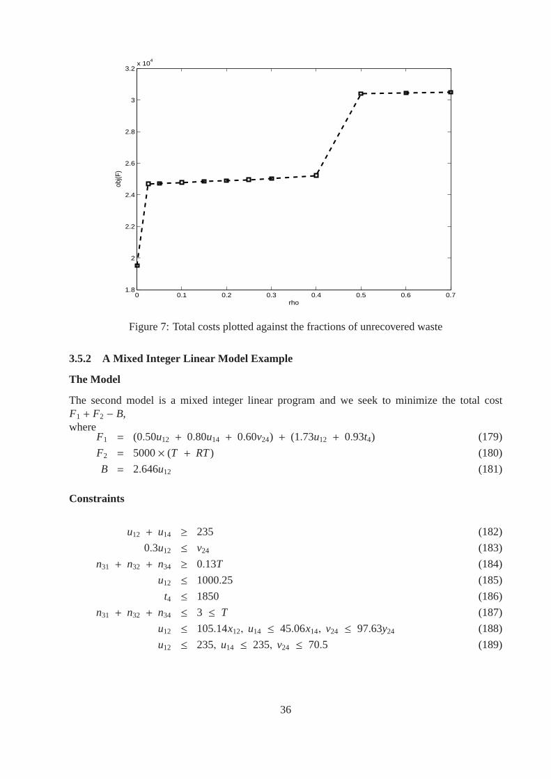
0 0.1 0.2 0.3 0.4 0.5 0.6 0.71.8

2

2.2

2.4

2.6

2.8

3

3.2x 10

4

rho

obj(F

)

Figure 7: Total costs plotted against the fractions of unrecovered waste

3.5.2 A Mixed Integer Linear Model Example

The Model

The second model is a mixed integer linear program and we seekto minimize the total costF1 + F2 − B,where

F1 = (0.50u12 + 0.80u14 + 0.60v24) + (1.73u12 + 0.93t4) (179)

F2 = 5000× (T + RT ) (180)

B = 2.646u12 (181)

Constraints

u12 + u14 ≥ 235 (182)

0.3u12 ≤ v24 (183)

n31 + n32 + n34 ≥ 0.13T (184)

u12 ≤ 1000.25 (185)

t4 ≤ 1850 (186)

n31 + n32 + n34 ≤ 3 ≤ T (187)

u12 ≤ 105.14x12, u14 ≤ 45.06x14, v24 ≤ 97.63y24 (188)

u12 ≤ 235, u14 ≤ 235, v24 ≤ 70.5 (189)

36

Variable Conditions

u12, u14, v24 ≥ 0 (190)

x12, x14, y24 integer ≥ 0 (191)

n31, n32, n34 integer ≥ 0 (192)

Definitions

t4 = u14 + v24 (193)

T = x12 + x14 + y24 (194)

RT = n31 + n32 + n34 (195)

The Solution

Let us first suppose that all the waste of 235 tons is carried from node 1 to node 2 (see Figure 8).We determine the number of trucks required to carry this waste from node 1 to node 2 and thenfrom node 2 to node 4, using inequalities (188).

m

m

-

?=

6

1 2

34

0.30

0.40

0.90

0.60

0.80

0.50

Figure 8: The fourth representation of the model.

We note thatu12 = 235, u14 = 0, v24 = 0.3× 235= 70.5. Thereforex12 = ⌈235/105.14⌉ = 3 andy24 = ⌈70.5/97.63⌉ = 1. So the the total number of trucks required to transport thewaste of 235from node 1 to node 2, and then the waste of 0.3× 235 tons from node 2 to node 4, using equation(194), isT = 4.

To obtain the required number of replacement trucks we use inequalities (184) and (187), andobtain

0.52 ≤ n31 + n32 + n34 ≤ 4

Since, from equation (195),RT = n31+ n32+ n34, it is reasonable to takeRT = ⌈0.52⌉ = 1.It is important to note that although an upper boundT on n31 + n32 + n34 is reasonable, it is not

the only one; the upper bound can be less or greater thanT .Since the waste at node 1 is transported to the incinerator atnode 2, the transportation cost of

0.50 per ton and a handling fee of 1.73 per ton are incurred. There are benefits of 3.78 per ton; so

37

the cost is

0.50 × 235 + 1.73 × 235 − 235 × 0.7 × 3.78 = − 97.76.

A proportion, 0.3 of the waste taken to the incinerator has to be moved to the landfill at 4 at a costof 0.60 per ton in addition to the handling charges at 4 of 0.93 per ton. The cost is therefore

0.3 × 235 × 0.60 + 0.3 × 235 × 0.93 = 107.865.

The cost for buying the trucks is 5000× (4+ 1) = 25,000. Thus the total cost is

25,000− 97.76 + 107.865 = 25,010.105.

Since there are benefits at node 2, the optimal cost is possibly 25,010.105; we check this claimby considering integral combinations of 4 (sinceT = 4). We note that the maximum number oftrucks that can be used to move the waste from node 1 to node 2 is3, and no more than 1 truck canbe used to carry the waste from node 2 to node 4.

(i) If two trucks are used to carry the waste from node 1 to node2, and one truck is used to movethe waste from node 2 to node 4, some waste will remain at node 1and has to be movedto node 4. The waste moved to node 2 is 7.51 × 14 × 2 = 210.8 tons leaving a balanceof 24.72 tons at node 1 that must be carried to node 4 usingx14 = ⌈24.72/(7.51 × 6)⌉ = 1truck. T = 4 andRT = ⌈0.52⌉ = 1; thus the total costF1 + F2 − B is

0.50× 210.8 + 0.80× 24.72 + 1.73× 210.8− 0.7× 210.8× 3.78 + (0.3× 210.8× 0.6

+ 5000× (4+ 1) = 25,028.6172.

(ii) If one truck is used to move the waste from node 1 to node 2,and one truck is used to carrythe waste from node 2 to node 4, some waste remains at node 1 andhas to be moved to node4. With one truck from node 1 to node 2, the waste carried to node 2 is 7.51 × 14 × 1 =105.14 tons leaving a balance of 129.86 tons at node 1 which must be moved to node 4 usingx14 = ⌈129.86/(7.51 × 6)⌉ = 3 trucks. T = 5 andRT = ⌈0.65⌉ = 1; thus the total costF1 + F2 − B is

(0.50 × 105.14+ 0.80 × 129.86− 0.7 × 105.14× 3.78) + 0.3 × 105.14 × 0.60+ 0.3×

105.14× 0.93+ 5000× (5+ 1) = 29,926.51682.

(iii) If all the waste at node 1 is now transported to node 4, then from inequalities (188),x14 =

⌈235/(7.51 × 6)⌉ = 6. SoT = 6 andRT = ⌈0.78⌉ = 1. In this case the total costF1+ F2− Bis

0.80× 235+ 0.93× 235+ 5000× (6+ 1) = 35,406.55.

Hence, the claimed optimal solution is indeed an optimal solution to the problem. As noted at theend of example1,T ≤ 3 is not possible because in this case waste will remain at node 1 which, iscontrary to the desired goal. Also,T ≥ 7 is obviously undesirable because some trucks will thenbe redundant. The optimal solution has been validated usingAMPL/CPLEX, and a Pentium IV2.66 GHz computer in less than two seconds.

38

Sensitivity Analysis

The optimal solutions for the mixed integer model asρ varies over the interval [0.0, 0.6] can befound in the same way as for the integer model. The reasoning is also similar to that used to find theoptimal solution for the mixed integer model just above; so only the optimal solutions are presentedfor the mixed integer model. The hand computed optimal solutions whenρ is respectively equalto 0.0,0.025, and 0.05 are stated just below. The remaining values found using AMPL/CPLEXare presented in Table 2. A graphical illustration of the behaviour of the total cost function asρvaries over the interval [0.0, 0.6] is given in Figure 9. It isobserved that the total cost falls withlower values ofρ; this is because the lowerρ is the more efficient the incinerator at node 2 is, andconsequently the more benefits will be obtained. The performance of both models can as well becompared from this figure. In general, the values of the objective functions are close to each otherexcept whenρ = 0.5; the big difference in values here is due to the fact that the integer modelusesone more truck that costs more money to buy (see Tables 1 and 2).

The extra truck is “used” in transporting extra “waste” fromnode 2 to node 4 (see Table 1).Whenρ = 5, there is increased “waste” from node 1 to node 2 which results in increased benefitsfrom node 2; this should not happen since the quality of the incinerator is getting worse. Howeverthis strange behaviour consists in the fact that the waste carried is determined by the trucks used,and since there may be some benefit (even if the incinerator isgetting worse) some pseudo wasteis likely to be transported on partially full trucks in orderto keep the total transportation costslower. Such strange isolated cases may not be many but they are likely to happen, and it is noteasy to put control constraints, because of the assumption that the trucks leave the waste collectionpoints when they are fully loaded. The best control may be to relax these assumptions by havingcontinuous variables to measure the amount of waste carried; in this case it may be easier to controlwhat is being transported as observed in the mixed integer linear model.

(i) We note that whenρ = 0.000 the equation (181) changes to

B = 3.78 × u12 (196)

and inequality (183) becomes

0 × u12 ≤ v24 (197)

The optimal solution is found to beu12 = 235, u14 = 0, v24 = 0, x12 = 3, x14 = 0, y24 = 0, andthe total cost is 19,635.75 with T = 3 andRT = 1.

(ii) If insteadρ = 0.025, the equation (181) changes to

B = 3.78 × 0.975 × u12 (198)

and inequality (183) becomes

0.025 × u12 ≤ v24 (199)

The optimal solution is found to beu12 = 235, u14 = 0, v24 = 5.875, x12 = 3, x14 = 0, y24 = 1,and the total cost is 24,666.94625 withT = 4 andRT = 1.

39

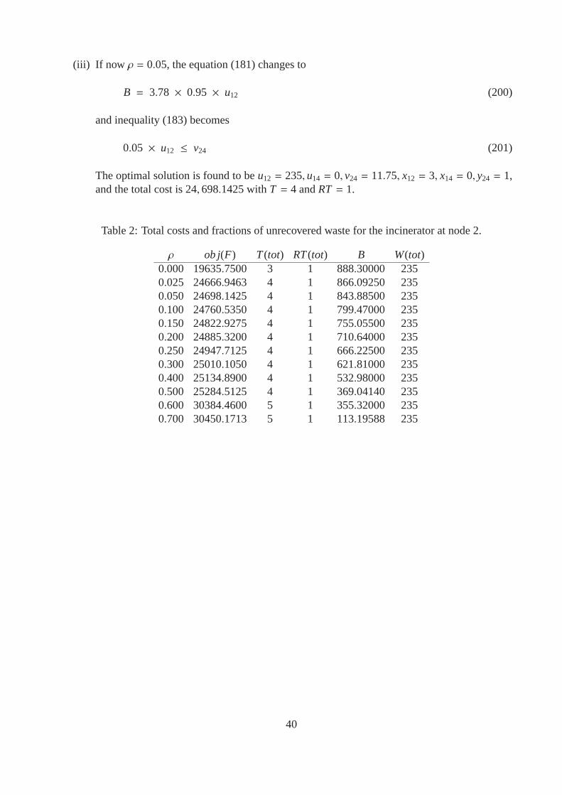
(iii) If now ρ = 0.05, the equation (181) changes to

B = 3.78 × 0.95 × u12 (200)

and inequality (183) becomes

0.05 × u12 ≤ v24 (201)

The optimal solution is found to beu12 = 235, u14 = 0, v24 = 11.75, x12 = 3, x14 = 0, y24 = 1,and the total cost is 24,698.1425 withT = 4 andRT = 1.

Table 2: Total costs and fractions of unrecovered waste for the incinerator at node 2.

ρ ob j(F) T (tot) RT (tot) B W(tot)0.000 19635.7500 3 1 888.30000 2350.025 24666.9463 4 1 866.09250 2350.050 24698.1425 4 1 843.88500 2350.100 24760.5350 4 1 799.47000 2350.150 24822.9275 4 1 755.05500 2350.200 24885.3200 4 1 710.64000 2350.250 24947.7125 4 1 666.22500 2350.300 25010.1050 4 1 621.81000 2350.400 25134.8900 4 1 532.98000 2350.500 25284.5125 4 1 369.04140 2350.600 30384.4600 5 1 355.32000 2350.700 30450.1713 5 1 113.19588 235

40

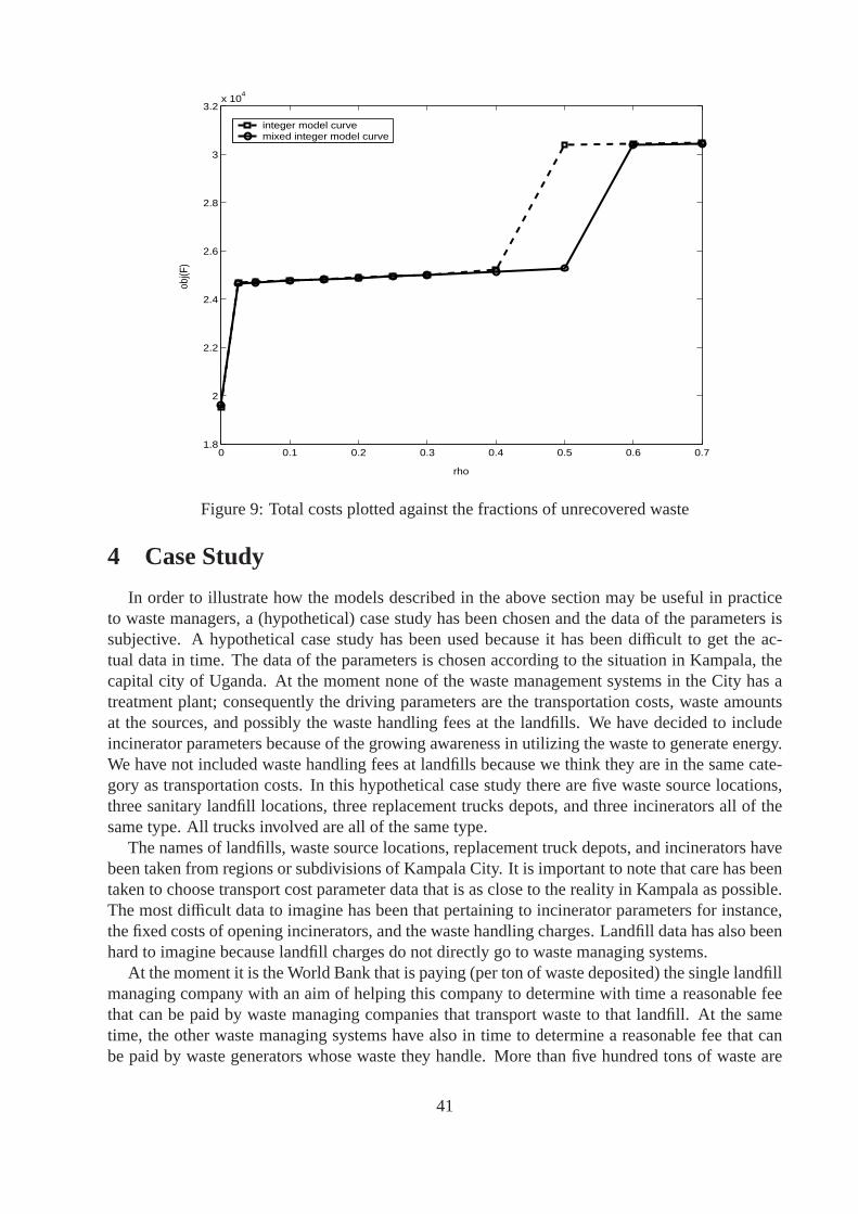
0 0.1 0.2 0.3 0.4 0.5 0.6 0.71.8

2

2.2

2.4

2.6

2.8

3

3.2x 10

4

rho

obj(F

)

integer model curvemixed integer model curve

Figure 9: Total costs plotted against the fractions of unrecovered waste

4 Case Study

In order to illustrate how the models described in the above section may be useful in practiceto waste managers, a (hypothetical) case study has been chosen and the data of the parameters issubjective. A hypothetical case study has been used becauseit has been difficult to get the ac-tual data in time. The data of the parameters is chosen according to the situation in Kampala, thecapital city of Uganda. At the moment none of the waste management systems in the City has atreatment plant; consequently the driving parameters are the transportation costs, waste amountsat the sources, and possibly the waste handling fees at the landfills. We have decided to includeincinerator parameters because of the growing awareness inutilizing the waste to generate energy.We have not included waste handling fees at landfills becausewe think they are in the same cate-gory as transportation costs. In this hypothetical case study there are five waste source locations,three sanitary landfill locations, three replacement trucks depots, and three incinerators all of thesame type. All trucks involved are all of the same type.

The names of landfills, waste source locations, replacementtruck depots, and incinerators havebeen taken from regions or subdivisions of Kampala City. It isimportant to note that care has beentaken to choose transport cost parameter data that is as close to the reality in Kampala as possible.The most difficult data to imagine has been that pertaining to incineratorparameters for instance,the fixed costs of opening incinerators, and the waste handling charges. Landfill data has also beenhard to imagine because landfill charges do not directly go towaste managing systems.

At the moment it is the World Bank that is paying (per ton of waste deposited) the single landfillmanaging company with an aim of helping this company to determine with time a reasonable feethat can be paid by waste managing companies that transport waste to that landfill. At the sametime, the other waste managing systems have also in time to determine a reasonable fee that canbe paid by waste generators whose waste they handle. More than five hundred tons of waste are

41

deposited everyday at the only landfill at Kiteezi; it is estimated that this is less than half of thetotal amount of waste accumulated daily in the entire city.

4.1 Data used to test the Models

The data for the parameters is given in Tables 3-18, that are given below. This data has also beenused to study the validity and robustness of the models described in Section 3. Tables 19-22 andFigures 10-13 give the findings from the sensitivity analysis tests conducted on total expenditureagainst the amount of waste at the sources, transportation costs, the fractions of waste that remainsat the incinerators, and the benefits from the incinerators.In Table 3 the locations for waste sources,sanitary landfills, replacement trucks depots, and incinerators are given. Table 4 gives waste source

Table 3: Node types and their locations

node type locationswaste sources (i) Kamwokya Kireka Ntinda Nalya Kiwatulelandfill (k) Kiteezi Namugongo Najeeratruck depot (r) Kyambogo Nakasero Lugogoincinerator (j) Kawempe Kiwatule Kasubi

locations as well as the waste amounts (in tons) at these locations. Table 5 gives the incinerator

Table 4: Waste amounts at waste sources.

waste source location (i) waste amount, di (in tons)Kamwokya 250.0Kireka 350.0Ntinda 400.0Nalya 245.7Kiwatule 268.5

locations j with their respective capacitiesQ j in tons, costs for treating a ton of waste ˜γ j, fixedcosts in opening these incineratorsδ j, and revenues per ton of waste at these incinerators ˜c j. Table

Table 5: Capacities, costs of opening and waste handling, revenues from incinerators.

j Q j δ j γ j c j

Kawempe 1200.00 975 1.57 1.67Kiwatule 1500.25 1079 1.73 6.78Kasubi 1300.50 1354 1.96 1.89

6 gives the landfill locationsk as well as landfill capacitiesQk, fixed costsδk incurred in openingthese landfills or tips, and costs ¯γk in handling a ton of waste at these landfills. Table 7 gives thereplacement trucks depots locationsr as well as fixed costsδr in opening them, and their capacitiesQr in terms of the number of trucks that can be kept in them. For simplicity we only have one type

42

of trucks. In Table 8 truck capacity in tonsαl, the probabilitypl of a truck breaking down in a day,and the costfl of buying a new truck are given. Table 9 gives the incineratorlocations j, and theproportions of wasteρ j that cannot be recovered by these incinerators. The waste that remains hasto be disposed of at landfills. In Table 10 waste source locationsi and sanitary landfill locationskare given. Transportations costs per tripcl

ik made by a truck from waste sources to landfills havealso been included. In Table 11 waste source locationsi and landfill locationsk are given. Theexpected number of tripsal

ik a truck can make per day between a waste sourcei and a landfillkare also given. Table 12 gives waste source locationsi and incinerator locationsj. Transportation

Table 6: Landfill locations, landfill capacities, costs of opening landfills, and unit waste handlingcharges.

k Qk δk γk

Kiteezi 1850 1500 0.93Namugongo 2500 1470 1.06Najeera 3750 1575 1.10

Table 7: Replacement trucks depot locations as well as their capacities and fixed costs in openingthem.

r δr Qr

Kyambogo 545.7 5Nakasero 590.3 7Lugogo 587.5 9

Table 8: Truck capacity, breakdown probability, and truck cost.

αl pl fl

7.51 0.13 5500

Table 9: Incinerator locations and waste proportions that remain at these incinerators.

j ρ j

Kawempe 0.3Kiwatule 0.3Kasubi 0.3

Table 10: Transportation costs between waste sources and landfills.

k\i Kamwokya Kireka Ntinda Nalya KiwatuleKiteezi 0.70 0.70 0.80 0.80 0.80Namugongo 0.70 0.50 0.60 0.40 0.50Najeera 0.60 0.70 0.80 0.60 0.60

43

costscli j per ton of waste per day from a waste source to an incinerator are given as well. Table 13

gives waste source locationsi and incinerator locationsj. It also gives the expected number of tripsai j a truck can make per day between a waste sourcei and an incineratorj. Table 14 gives landfilllocationsk and incinerator locationsj. Transportation costscl

jk per ton of waste from incineratorsto landfills are also given. In Table 15 incineratorj and landfillk locations are provided. Theexpected number of tripsbl

jk a truck can make everyday between incineratorj and landfillk arealso given. Table 16 gives replacement trucks depotsr and landfillk locations. Transportation costs

Table 11: Expected number of trips a truck makes per day between a waste sources and a landfills.

k\i Kamwokya Kireka Ntinda Nalya KiwatuleKiteezi 8 9 6 5 5Namugongo 9 14 12 15 14Najeera 12 8 7 13 12

Table 12: Transportation costs between waste sources and incinerators.

j\i Kamwokya Kireka Ntinda Nalya KiwatuleKawempe 0.60 0.80 0.60 0.60 0.60Kiwatule 0.50 0.70 0.50 0.50 0.40Kasubi 0.70 0.90 0.70 0.70 0.70

Table 13: Expected number of trips a truck can make a day between a waste source and an incin-erator.

j\i Kamwokya Kireka Ntinda Nalya KiwatuleKawempe 13 8 12 12 11Kiwatule 14 10 14 14 17Kasubi 10 4 4 8 8

Table 14: Transportation costs between incinerators and landfills.

j\k Kiteezi Namugongo NajeeraKawempe 0.40 0.60 0.70Kiwatule 0.60 0.70 0.60Kasubi 0.60 0.80 0.70

Table 15: Expected number of trips a truck can make a day between an incinerator and a landfill.

j\k Kiteezi Namugongo NajeeraKawempe 17 12 10Kiwatule 13 10 13Kasubi 11 7 6

44

clrk from depots to landfills are also given. In Table 17 replacement trucks depotsr and incinerator

Table 16: Transportation costs between replacement trucksdepots and landfills.

r\k Kiteezi Namugongo NajeeraKyambogo 0.90 0.70 0.70Nakasero 0.80 0.70 0.80Lugogo 0.90 0.70 0.90

j locations are provided. Transportation costs ¯clr j from a depotr to an incineratorj are also given.

Table 18 provides transportation costs of moving replacement trucks between their depotsr and

Table 17: Transportation costs between replacement trucksdepots and incinerators.

r\ j Kawempe Kiwatule KasubiKyambogo 0.70 0.40 0.80Nakasero 0.60 0.60 0.70Lugogo 0.70 0.50 0.80

waste sourcesi.

Table 18: Transportation costs between replacement trucksdepots and waste sources.

r\i Kamwokya Kireka Ntinda Nalya KiwatuleKyambogo 0.50 0.40 0.30 0.30 0.20Nakasero 0.50 0.70 0.60 0.70 0.60Lugogo 0.30 0.50 0.60 0.60 0.60

4.2 Solution, Validity and Robustness of the First Model

The solution to the model has been obtained using a Pentium IV2.66 GHz computer in less thantwo seconds. All data from the previous section has been usedin the validity test; only some of ithas been used in the robustness tests. The reason is that in the robustness tests the attention has beenmore on the sensitivity to changes in some of the most important parameters as far as the situationof Kampala is concerned. Also, some of the data is in the same category like the transportationcosts between waste sources and incinerators, and the transportation costs between incineratorsand landfills, etc. In particular the following parameters and functions have been studied; revenuefrom an incinerator at Kiwatulerev(kiw), total costsob j(F), total truck number used per dayT (tot), total replacement trucks number used per dayRT (tot), waste amount a sourcewaste(amt)in Ntinda, total waste amount collected from all waste sources per dayW(tot), fractionsρ of wastethat remains per day at incinerators, and transportation costs from a waste source at Kamwokyaand a landfill (tip) at Najeera.

The changes in the parametersrev(kiw), waste(amt), ρ, and the transportation cost betweenKamwokya and Najeera have been studied against the total cost ob j(F). The findings are given in

45

Tables (19)-(22), and graphically depicted in Figures (10)-(13). The graphs in these figures havebeen plotted using matlab 6.5.

The validity of the model has been tested by doubling the values of the parameters except forthe values of waste fractions that remain at incinerators and the daily truck breakdown probability.This has not affected the values of the decision variables; it has also indicated that the model hasbeen well formulated.

The robustness of the model described in Section 3.1 has beenstudied by looking at the changesin some of the key parameters; revenues at an incinerator at Kiwatule, waste source amountsat Ntinda, transportation costs between a waste source at Kamwokya and a landfill at Najeera,changes in the fractions of wastes that is unrecovered at an incinerator at Kiwatule. The changes inthese parameters have specifically been observed with respect to total costs; changes in other datalike total waste amount from all waste sources every dayW(tot) have also been reflected as shownin the tables below. The changes in these parameters have been significant and they have greatlyaffected the total cost; small changes have induced small changes while big changes have causedbig changes in the total cost.

Part of the solution from the case study is shown in the fifth row from the top of Table 19.Since our decision variables measure truck numbers, the sharpness of this solution can be studiedby looking at the total amount of waste collected per day fromall sources; the actual total wasteamount from all waste sources is 1514.2 tons. From Table 19 itis given as 1659.71 tons whenrev(kiw) is 6.78, giving a deviation of 145.51 tons from the actual value. In general, the biggestdeviation has been observed to be 243.14 tons in Table 22 whenthe total waste from all sourcesis given as 1757.34 tons. This inflation in waste amounts is also observed in the total costob j(F)and the benefitsB.

The observed inflation consists in the assumption that the trucks leave the waste collectionpoints when they are fully loaded. Some of these trucks may actually be partially full; so there is anoverestimation if the truck number is simply multiplied by the truck capacity to obtain the amountof waste collected. This problem has been overcome by using the modified model described inSection 3.3. The results from using that model are given in Tables 23-26, and Figures 14-17.

Table 19 represents the relationship between the total costob j(F) and the income per ton ofwasterev(kis) from the incinerator at Kiwatule. As the revenue in the interval [4.78, 9.98] in-creases, the total costob j(F) decreases. The change in the revenue affects also the benefitsB;there are no benefits if the value ofrev(kiw) is at most equal to 6.28. The relationship betweenob j(F) andrev(kiw) is shown in Figure 10; this figure shows that as the revenue increases, the totalcost reduces. The total cost does not change when the benefitsare at most 6.28 per ton of waste;in this case no waste is taken for incineration because it is not economically profitable.

Table 20 shows a variation in the total costob j(F) with the variation in the waste amountwaste(amt) at a source in Ntinda over the interval [300, 500]. The totalcost increases with anincrease in waste amount. The variation inwaste(amt) also affectsT (TOT ) butRT (TOT ) remainsstable. However, small changes in the values ofwaste(amt) cause small changes in the values ofFandT (TOT ) over this interval. The relationship betweenF andwaste(amt) is depicted in Figure11; it is clear from the graph that the values ofob j(F) are increasing with the values ofwaste(amt).

Table 21 shows a variation in the values ofob j(F) with respect to changes in the transportationcostc(soti) between a waste source at Kamwokya and a landfill at Najeera over the interval [0.10,21.00]. It is clear from the table that the higher the transportation costs the higher the total costs.There are slight changes in the values ofT (TOT ) andB. The values ofRT (TOT ) do not changewhile the values ofW(tot) change slightly. The relationship betweenF and c(soti) is given inFigure 12; it is evident from the graph that when eventually the cost to Najeera landfill is very high

46

Table 19: Total costs and benefits from Kiwatule.

rev(kiw) ob j(F) T (tot) RT (tot) B W(tot)4.78 121803.010 18 3 0000.00000 1667.225.28 121803.010 18 3 0000.00000 1667.225.78 121803.010 18 3 0000.00000 1667.226.28 121803.010 18 3 0000.00000 1667.226.78 121705.704 18 3 1496.98332 1659.717.28 121595.307 18 3 1607.38032 1659.717.78 121484.910 18 3 1717.77732 1659.718.28 121374.513 18 3 1828.17432 1659.718.78 121264.116 18 3 1938.57132 1659.719.28 121153.719 18 3 2048.96832 1659.719.98 120999.163 18 3 2203.52412 1659.71

4 5 6 7 8 9 101.209

1.21

1.211

1.212

1.213

1.214

1.215

1.216

1.217

1.218

1.219x 10

5

rev(kiw)

obj(F

)

Figure 10: Total cost plotted against benefits from incineration

47

Table 20: Total costs and waste amounts at Ntinda.

waste(amt) ob j(F) T (tot) RT (tot) B W(tot)300 116018.254 17 3 1496.98332 1547.060320 116153.411 17 3 0000.00000 1577.100340 116203.127 17 3 0000.00000 1614.650360 116203.127 17 3 0000.00000 1614.650380 121667.853 18 3 1496.98332 1637.180400 121705.704 18 3 1496.98332 1659.710420 121852.726 18 3 0000.00000 1704.770440 121852.726 18 3 0000.00000 1704.770460 127136.186 19 3 1496.98332 1697.260480 127317.452 19 3 1496.98332 1727.300500 127452.609 19 3 0000.00000 1754.340

300 320 340 360 380 400 420 440 460 480 5001.16

1.18

1.2

1.22

1.24

1.26

1.28x 10

5

waste(amt)

obj(F

)

Figure 11: Total cost plotted against waste amount at Ntinda

48

no waste will deposited there and consequently any further increments in the cost will not affectthe total cost.

Table 21: Total costs and transportation costs from Kiwatule waste source to Kiteezi landfill.

c(soti) ob j(F) T (tot) RT (tot) B W(tot)0.10 121570.524 18 3 1496.98332 1659.7100.30 121624.596 18 3 1496.98332 1659.7100.60 121705.704 18 3 1496.98332 1659.7100.80 121759.776 18 3 1496.98332 1659.7101.00 121813.848 18 3 1496.98332 1659.710

10.00 124247.088 18 3 1496.98332 1659.71015.00 125598.888 18 3 1496.98332 1659.71017.00 125878.697 19 3 2993.96664 1629.67019.00 125878.697 19 3 2993.96664 1629.67021.00 125878.697 19 3 2993.96664 1629.670

0 5 10 15 20 251.215

1.22

1.225

1.23

1.235

1.24

1.245

1.25

1.255

1.26x 10

5

c(soti)

obj(F

)

Figure 12: Total cost plotted against transportation costsfrom Kiwatule to Kiteezi

Table 22 shows the variation in the values ofob j(F) with respect to changes in the values ofρin the interval [0.0, 0.6]. It is clear from the table that thelower the value ofρ, the lower the totalcosts. There are slight changes in the values ofT (tot) but RT (tot) remains stable. There may beno benefits if the value ofρ is at least equal to 0.4; this is shown in the table and in Figure 13. Agraphical relationship betweenob j(T ) andρ is given in Figure 13; it is evident from the graph thatthe lowerρ is the lower the total cost. This means that the better the quality of the incinerators the

49

Table 22: Total costs and fractions of unrecovered waste at incinerators

ρ ob j(F) T (tot) RT (tot) B W(tot)0.000 106803.046 17 3 10030.80660 1757.340.025 112685.992 18 3 9780.03643 1757.340.050 112936.762 18 3 9529.26627 1757.340.100 117459.517 18 3 4490.94996 1742.320.150 119587.758 18 3 3635.53092 1629.670.200 120769.988 18 3 2525.52288 1644.690.250 121291.242 18 3 1985.79420 1674.730.300 121705.704 18 3 1496.98332 1659.710.400 121803.010 18 3 0000.00000 1667.220.500 121803.010 18 3 0000.00000 1667.220.600 121803.010 18 3 0000.00000 1667.22

0 0.1 0.2 0.3 0.4 0.5 0.6 0.71.06

1.08

1.1

1.12

1.14

1.16

1.18

1.2

1.22x 10

5

rho

obj(F

)

Figure 13: Total costs plotted against fractions of unrecovered waste

50

lower the expenditure; eventually if the quality of the incinerators is very bad then there will be nogain at all.

These tests and the graphical observations have indicated that the model is satisfactorily robust.The nature of the graphs in figures 10, 11, 12, and 13 is not surprising since the objective functionof the model described in Section 3.1 is a linear combinationof convex functions defined overconvex sets. The variables in the model are integer; if they were to be continuous then a piecewiselinear appearance would be depicted in the graphs. This would be so because of the piecewiselinearity of the functions involved (see Murty [50]) in the objective function. The graphs in Figures(10)-(13) are composed of discrete points that have been joined by lines in order to show the trendof the plots.

4.3 Solution, Validity, and Robustness of the Second Model

In this section we present the solution to the second model, as well as the findings from thesensitivity analysis tests conducted on the first model described in Section 3.1 and the secondmodel described in Section 3.3.

The solution to the model has been obtained using a Pentium IV2.66 GHz computer in lessthan five seconds. Sensitivity analysis tests have been conducted on the second model over thesame intervals of data like in the case of the first model. The findings are summarized in Tables23-26; the number of trucks given in these tables is, in general, the same as that given in Tables19-22 for the first model. The graphical comparison of the twomodels is given in Figures 14-17.The second model gives superior values of the total cost and the amount of waste at the collectionpoints.

Table 23 gives the variation of the total cost with respect tothe change in the revenue from theincinerator at Kiwatule, over the interval [4.78, 9.78]. The total cost falls with an increase in therevenue; this is also the case for the first model. Figure 14 compares the differences in the totalcost for the two models; the second model gives much better total cost values.

Table 23: Total costs and benefits from Kiwatule.

rev(kiw) ob j(F) T (tot) RT (tot) B W(tot)4.78 121504.482 18 3 0000.00000 1514.25.28 121504.482 18 3 0000.00000 1514.25.78 121504.482 18 3 0000.00000 1514.26.28 121504.482 18 3 0000.00000 1514.26.78 121427.152 18 3 1496.98332 1514.27.28 121316.755 18 3 1607.38032 1514.27.78 121206.358 18 3 1717.77732 1514.28.28 121095.961 18 3 1838.17432 1514.28.78 120985.564 18 3 1938.57132 1514.29.28 120875.167 18 3 2048.96832 1514.29.78 120764.770 18 3 2159.36532 1514.2

Table 24 gives the relationship between the total cost and the waste amount at Ntinda, as thewaste amount is varied over the interval [300, 500]. It is evident from the table and Figure 15 thatthe total cost increases with the waste amount. It is clear from the Figure that the two models havevery close total cost values.

51

4 5 6 7 8 9 101.206

1.208

1.21

1.212

1.214

1.216

1.218

1.22x 10

5

rev(kiw)

obj(F

)first model curvesecond model curve

Figure 14: Total cost plotted against benefits from incineration

Table 24: Total costs and waste amounts at Ntinda.

waste(amt) ob j(F) T (tot) RT (tot) B W(tot)300 115724.443 17 3 1544.50660 1414.2320 115871.682 17 3 0000.00000 1434.2340 115904.882 17 3 0000.00000 1454.2360 115938.082 17 3 0000.00000 1474.2380 121357.118 18 3 1544.50660 1494.2400 121427.152 18 3 1496.98332 1514.2420 121537.682 18 3 0000.00000 1534.2440 121570.882 18 3 0000.00000 1554.2460 126896.975 19 3 1544.50660 1574.2480 127023.243 19 3 1544.50660 1594.2500 127170.482 19 3 0000.00000 1614.2

52

300 320 340 360 380 400 420 440 460 480 5001.14

1.16

1.18

1.2

1.22

1.24

1.26

1.28x 10

5

waste(amt)

obj(F

)

first model curvesecond model curve

Figure 15: Total cost plotted against waste amount at Ntinda

Table 25 gives the relationship between the total cost and the changes in the transportation costbetween a waste source at Kamwokya and a landfill at Najeera, over the interval [0.10, 21.00].The table and Figure 16 show that the total cost increases with the transport cost. Again in thiscase, the second model gives much better total cost values than the first model. The gap betweenthe total costs of the two models increases with the transportation cost. This is because the wasteamounts are steadily inflated in the integer model (see Tables 21 and 25) so that as the transporta-tion cost increases the gap between the two objective functions inevitably increases. The realistictransportation cost values lie between 0 and 1.5; the values of the interval between 10 and 21 wereonly considered to check whether the model does what is expected of it as the cost grows.

Table 25: Total costs and transportation costs from Kiwatule waste source to Kiteezi landfill.

c(soti) ob j(F) T (tot) RT (tot) B W(tot)0.10 121302.152 18 3 1496.98332 1514.20.30 121352.152 18 3 1496.98332 1514.20.60 121427.152 18 3 1496.98332 1514.20.80 121477.152 18 3 1496.98332 1514.21.00 121527.152 18 3 1496.98332 1514.2

10.00 123777.152 18 3 1496.98332 1514.215.00 124677.971 19 3 2376.16400 1514.217.00 124677.971 19 3 2376.16400 1514.219.00 124677.971 19 3 2376.16400 1514.221.00 124677.971 19 3 2376.16400 1514.2

53

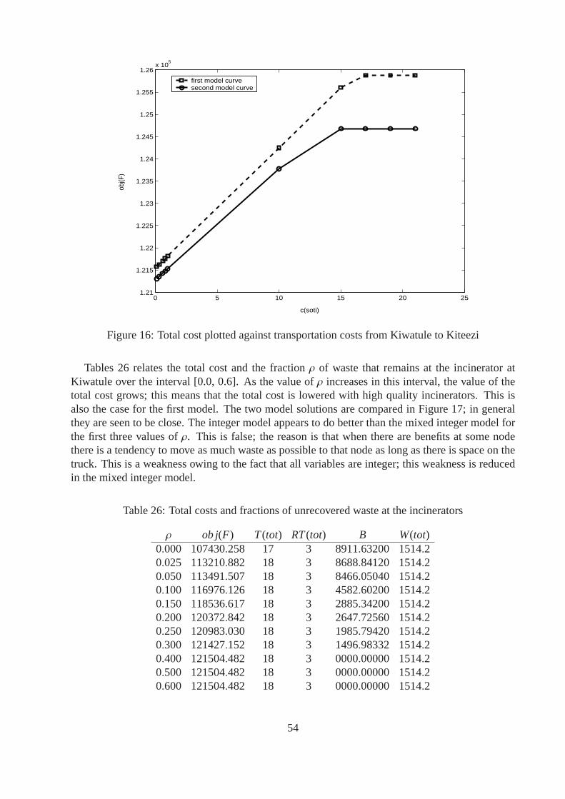
0 5 10 15 20 251.21

1.215

1.22

1.225

1.23

1.235

1.24

1.245

1.25

1.255

1.26x 10

5

c(soti)

obj(F

)

first model curvesecond model curve

Figure 16: Total cost plotted against transportation costsfrom Kiwatule to Kiteezi

Tables 26 relates the total cost and the fractionρ of waste that remains at the incinerator atKiwatule over the interval [0.0, 0.6]. As the value ofρ increases in this interval, the value of thetotal cost grows; this means that the total cost is lowered with high quality incinerators. This isalso the case for the first model. The two model solutions are compared in Figure 17; in generalthey are seen to be close. The integer model appears to do better than the mixed integer model forthe first three values ofρ. This is false; the reason is that when there are benefits at some nodethere is a tendency to move as much waste as possible to that node as long as there is space on thetruck. This is a weakness owing to the fact that all variablesare integer; this weakness is reducedin the mixed integer model.

Table 26: Total costs and fractions of unrecovered waste at the incinerators

ρ ob j(F) T (tot) RT (tot) B W(tot)0.000 107430.258 17 3 8911.63200 1514.20.025 113210.882 18 3 8688.84120 1514.20.050 113491.507 18 3 8466.05040 1514.20.100 116976.126 18 3 4582.60200 1514.20.150 118536.617 18 3 2885.34200 1514.20.200 120372.842 18 3 2647.72560 1514.20.250 120983.030 18 3 1985.79420 1514.20.300 121427.152 18 3 1496.98332 1514.20.400 121504.482 18 3 0000.00000 1514.20.500 121504.482 18 3 0000.00000 1514.20.600 121504.482 18 3 0000.00000 1514.2

54

0 0.1 0.2 0.3 0.4 0.5 0.6 0.71.06

1.08

1.1

1.12

1.14

1.16

1.18

1.2

1.22x 10

5

rho

obj(F

)

first model curvesecond model curve

Figure 17: Total costs plotted against fractions of unrecovered waste

55

5 AMPL and CPLEX

The AMPL modelling system is a comprehensive, powerful, algebraic modelling language forproblems in linear, non-linear, and integer programming. With AMPL models with maximumproductivity can be created, and by using AMPL’s natural algebraic notation, very large, complexmodels can be stated in a concise, understandable form. Since its models are easy to understand,debug, and modify, AMPL also makes model maintenance easy (see Fourer et al [23]). AMPL-compatible solvers include CPLEX, FortMP, MINOS, MINLP and others (see AMPL website:http://www.ampl.com). CPLEX is designed to solve linear programs, integer programs, mixedinteger programs, and quadratic programs.

5.1 Linear Programming

CPLEX employs either a simplex or a barrier method to solve linear programming problems.Four distinct methods of optimization are incorporated in the CPLEX package:

• A primal simplex algorithm that first finds a solution feasible in constraints (Phase I), theniterates towards optimality (Phase II).

• A dual simplex algorithm that finds a solution that satisfies the optimality conditions (PhaseI), then iterates towards feasibility (Phase II).

• A network primal simplex algorithm that uses logic and data structures tailored to the classof pure network linear programs.

• A primal-dual-barrier (or interior point) algorithm that simultaneously iterates toward feasi-bility and optimality, optionally followed by a primal or dual crossover routine that producesa basic optimal solution.

CPLEX normally chooses one of these algorithms, but its choice can be overridden by thedirectives described in the ILOG AMPL CPLEX system [41], pp 30-32. These directives (or spe-cific options) apply to the solution of linear programs, including network linear programs. Thereare also directives for processing, controlling the simplex algorithm, controlling the barrier algo-rithm, improving stability, starting and stopping, controlling output described in the ILOG AMPLCPLEX system [41], pp 32-44.

CPLEX is highly robust and has been designed to avoid problemssuch as degenerate stallingand numerical inaccuracy that occur in the simplex algorithm. However, some linear programs canbenefit from the adjustments to the stability directives if difficulties arise.

5.2 Integer Programming

For programs that contain integer variables, CPLEX uses a branch and bound approach. Be-cause a single integer program generates many integer program sub problems, even small instancescan be very computation-intensive and require significant amounts of memory. In contrast to solv-ing linear programming problems, where little user intervention is required to obtain optimal re-sults, some of the directives for preprocessing (see the ILOG AMPL CPLEX system, pp 47-50)may have to be set to get satisfactory results on integer programs. Either the way that the branchand bound algorithm works can be changed, or the conditions for optimality can be relaxed.

56

Other directives (see the ILOG AMPL CPLEX system [41], pp 50-60) include those for algo-rithmic control, relaxing optimality, halting and resuming the search, and controlling output. Allprocessing directives that apply to linear programming arealso applicable to problems that specifyinteger-valued variables. The directives on pp 47-50 control additional preprocessing steps that areapplicable to certain mixed integer program only.

In dealing with a difficult integer program, it may be better to settle for a “good” solution ratherthan a provably one. Directives for relaxing optimality, described on pages 56-57, offer variousways of weakening the optimality criterion for CPLEX’s branch and bound algorithm.

The most common problems faced in solving mixed integer programs with CPLEX are due torunning out of memory, failure to reach optimality, difficult mixed integer program sub problems.The problems and the ways to overcome them are described in the ILOG AMPL CPLEX system[41], pp 60-63.

6 Conclusions and future developments

An integer linear programming model and a mixed integer linear programming model havebeen proposed, and confirmed to be valid and robust. Their performance has been studied using ahypothetical case study, and other smaller models using AMPL/CPLEX. The mixed integer linearmodel has been found to be more precise in measuring waste flowamounts among various nodesin the model and total daily costs incurred in the managementof waste. However, the integer linearmodel cannot be discarded because the choice between the twomodels depends on the interest ofthe user. One user prefers to measure transportation costs in terms of costs per trip from a wastesource while another user wants to measure the transportation costs in terms of costs per unit massof waste moved from a waste source. The technology in place can as well influence the choice ofthe model to apply. For example in the Ugandan situation, where it is not possible at the momentto measure waste from waste sources, the integer linear model is more appropriate. In this case wereplace the coefficients of the variablesX andY in the objective function with the total costs per tripfrom the waste collection point. At the same time, instead ofmeasuring the amount of waste usingthe number of trucks used multiplied by their capacities, continuous variables can be introducedto measure directly the amount of waste that goes to the plants and landfills. The integer linearproblem is then transformed into a mixed integer problem that gives better total cost estimates andmore precise waste amount measurements.

Through these models it is not only possible to obtain waste amounts transported to variousfacilities, but also obtain the number of trucks as well as replacement trucks used in doing so. Themain pitfall of the integer linear model is due to the use of the number of trucks used to measurethe amount of waste transported; the values of the waste amounts, the total cost, and the values ofthe benefits from the plants may be inflated, since the trucks are assumed to be fully loaded uponleaving the waste collection points. Some of the trucks may in reality be partially full, and thisunexploited capacity leads to errors in computing the totalcosts, measuring waste amounts, and thebenefit values. The weakness common to both models is that theestimated values of the parametersmay not reflect the true behaviour of the parameters at the time of estimation. The findings indicatethat both models can be useful decision support tools in the planning and management of municipalsolid waste collection, transportation, incineration, recycling, composting, and disposal programs.They can as well be used as design tools for setting up plants,truck depots, and landfills.

The models may be useful in other areas of application. For instance, suppose an investor isopening an industry to produce various products. He also wants to open warehouses and find

57

agents for his products in some potential areas. He intends to use trucks of various capacity totransport the goods to the warehouses and to his agents. The problem may be that of opening andrunning warehouses, and distributing the goods among the agents at minimum transportation costs.The first model can be adapted by considering collection points as the industry and its branches,the plants can be taken for the warehouses, and the landfills can be the agents.

In the order of importance, the work is to be extended or modified in the following ways;

1. Robustness issues are to be examined more globally by studying the performance of themodels, under the changes in all key parameters. For instance we have studied the changesin the total costs with respect to the changes in the fractionof waste that remains at theincinerators, and these fractions have been assumed to be dependent on the incineratorsonly. We have not considered the dependence of these fractions on the type of waste.

2. Another consideration is that of extending the deterministic models to stochastic ones bytreating the data as a random variable because of random fluctuations in some of the keyparameters, like the amounts of waste at the collections points. In many real world problems,the yield or total expenditure, etc. is almost never known with certainty. It is a randomvariable that is subject to many random fluctuations that arenot under our control. Forexample the daily total expenses depend on transportation costs per unit waste, the quality ofthe plants, the amount of waste at the collection points, etc. To analyse the problem treatingthe yield as a random variable requires the use of stochasticprogramming models (Murty[51]). The construction of stochastic models can be done by making assumptions about thenature of the probability distributions of the random data elements, or by estimating thesedistributions from the past data. The challenge is that the closeness of the optimum solutionobtained from the model may depend on how close the selected probability distributions areto the true ones (Murty [51]).

3. The element of time (dynamic element) is to be introduced into the general models; forinstance we can consider daily activities within time period t = 1, . . . , T0, where someparameters can change with timet. Planning involves time, and if an application is concernedwith a situation that lasts for days or months or years, the same types of decisions may haveto be made everyday, for example (Murty [51]).

When planning a multi-period horizon (sayT0), and there is no change in the data at all fromone period to the next, then the optimum solution for the firstperiod found from the staticmodel for that period , will remain optimal for each period inthe planning horizon.

In most multi-period problems, data changes from period to the next are significant, and theoptimum decisions for the various periods may be different, and the sequence of decisionswill be interrelated. Designing a dynamic model with the aimof finding a sequence ofdecisions (one for every period) that is optimal for the planning horizon as a whole, requiresreasonably accurate estimates of data for every period of the planning horizon. This is achallenge, but if such data is available, a dynamic model tries to find the entire sequence ofinterrelated decisions that is optimal for the model over the entire planning horizon (Murty[51]).

58

References

[1] Alidi, A.S., 1992. An Integer Goal Programming Model forHazardous Waste Treatment andDisposal. Appl. Math. Modelling Vol. 16, 645-651.

[2] Amouzegar, M.A., Moshirvaziri, K., 2001. Strategic management decision support system:An analysis of the environmental policy issues. Environmental Modeling and Assessment 6,297-306.

[3] Badran, M.F. and El-Haggar, S.M., 2006. Optimization of Municipal Solid Waste Manage-ment in Port Said - Egypt. Waste Management 26, 534-545.

[4] Bloemhof-Ruwaard, J.M., Salomon, M., Wassenhove, L.N.V., 1996. The Capacitated Distri-bution and Waste Disposal Problem. European Journal of Operational Research 88, 490-503.

[5] Caruso, C., Colorni, A., Paruccini, M., 1993. The regional urban solid waste managementsystem: A modelling approach. European Journal of Operational Research 70, 16-30.

[6] Chang, Y.H., Chang, N.B., 1998. Optimization Analysis for the Development of Short-term Solid Waste Management Strategies using Presorting Process prior to Incinerators. Re-sources, Conservation and Recycling 24, 7-32.

[7] Chang, N.B., Chen, Y.L., Wang, S.F., 1997. A Fuzzy Interval Multi objective Mixed Inte-ger Programming Approach for the Optimal Planning of Solid Waste Management Systems.Fuzzy Sets and Systems 89, 35-60.

[8] Chang, N.B., Davila, E., Dyson, B., Brown, B., 2005. Optimal Design for Sustainable Devel-opment of Material Recovery Facility in a Fast-Growing UrbanSetting. Waste Management.Article in Press.

[9] Chang, N.B and Davila, E., 2006. Minimax regret optimization analysis for a regional solidwaste management system. Waste Management. Article in Press.

[10] Chang, N.B., Schuler, R.E. and Shoemaker, C.A. 1993. Environmental and Economic Op-timization of an Integrated Solid Waste Management System.Journal of Resource Manage-ment and Technology 21(2), 87-100.

[11] Chang, N.B., Shoemaker, C.A., Schuler, R.E., 1996. Solid Waste Management System Anal-ysis with Air Pollution and Leachate Impact Limitations. Waste Management & Research 14,463-481.

[12] Chang, N.B., Yang, Y.C., Wang, S.F., 1996. Solid-Waste Management System Analysis withNoise Control and Traffic Congestion Limitations. Journal of Environmental Engineering,Vol. 122, No. 2, 122-131.

[13] Chang, N.B., Wang, S.F., 1994. A Locational Model for the Site Selection of Solid WasteManagement Facilities with Traffic Congestion Constraints. Civil. Eng. syst., Vol. 11, 287-306.

[14] Chang, N.B., Wang, S.F., 1996. Solid Waste Management System Analysis by Multi objectiveMixed Integer Programming Model. Journal of EnvironmentalManagement 48, 17-43.

59

[15] Chang, N.B., Wang, S.F., 1996. Comparative Risk Analysis for Metropolitan Solid WasteManagement Systems. Journal of Environmental Management 20(1), 65-80.

[16] Chang, N.B., Wang, S.F., 1996. Managerial Fuzzy Optimal Planning for Solid-Waste Man-agement Systems. Journal of Environmental Engineering, Vol. 122, No. 7, 649-658.

[17] Chang, N.B., Wang, S.F., 1997. A Fuzzy Goal Programming Approach for the Optimal Plan-ning of Metropolitan Solid Waste Management Systems. European Journal of OperationalResearch 99, 303-321.

[18] Costi, P., Minciardi, R., Robba, M., Rovatti, M., Sacile, R.,2004. An environmentally sus-tainable decision model for urban solid waste management. Waste Management 24, 277-295.

[19] Daskalopoulos, E., Badr, O., Probert, S.D., 1998. An Integrated Approach to Solid WasteManagement. Resources, Conservation and Recycling 24, 33-50.

[20] Davila, E and Chang, N.B., 2005. Sustainable pattern analysis of a publicly owned materialrecovery facility in a fast-growing urban setting under uncertainty. Journal of EnvironmentalManagement 75, 337-251.

[21] Everett, J.W., Modak, A.R., 1996. Optimal Regional Scheduling of Solid Waste Systems. I:Model Development. Journal of Environmental Engineering,Vol. 122, No. 9, 785-792.

[22] Fiorucci, P., Minciardi, R., Robba, M., Sacile, R., 2003. Solid waste management in urbanareas development and application of a decision support system. Resources, Conservationand Recycling 37, 301-328.

[23] Fourer, R, Gay, D.M., Kernigham, B.W., 2003. AMPL: A Modeling Language for Mathe-matical Programming. Second Edition, Duxbury, Toronto, Canada.

[24] Ghose, M.K., Dikshit, A.K., Sharma, S.K., 2006. A GIS based transportation model for solidwaste disposal - A case study on Asansol municipality. WasteManagement 26, 1287-1293.

[25] Gottinger, H.W., 1986. A Computational Model for Solid Waste Management with Applica-tions. Appl. Math. Modelling, Vol. 10, 330-338.

[26] Gottinger, H.W., 1988. A Computational Model for Solid Waste Management with Applica-tions. European Journal of Operational Research 35, 350-364.

[27] Hasit, Y., Warner, D.B., 1981. Regional Solid Waste Planning with WRAP. Journal of Envi-ronmental Engineering Division, ASCE, Vol. 107, No. EE3, 511-525.

[28] Huang, Y.F., Baetz, B.W., Huang, G.H., Liu, L., 2002. Violation Analysis for Solid WasteManagement Systems: An interval fuzzy programming approach. Journal of EnvironmentalManagement 65, 431-446.

[29] Huang, G., Baetz, B.W., Patry, G.G., 1992. A Grey Linear Programming Approach for Mu-nicipal Solid Waste Management Planning under Uncertainty. Civil. Eng. Syst., Vol. 9, 319-335.

[30] Huang, G.H., Baetz, B.W., Patry, G.G., 1993. A Grey Fuzzy Linear Programming Approachfor Municipal Solid Waste Management Planning under Uncertainty. Civil. Eng. Syst., Vol.10, 123-146.

60

[31] Huang, G.H., Baetz, B.W., Patry, G.G., 1994. Waste Allocation Planning through a GreyFuzzy Quadratic Programming Approach. Civil. Eng. Syst., Vol. 11, 209-243.

[32] Huang, G.H., Baetz, B.W., Patry, G.G., 1994. Grey DynamicProgramming for Waste-Management Planning under Uncertainty. Journal of Urban Planning and Development,ASCE, 132-157.

[33] Huang, G.H., Baetz, B.W., Patry, G.G., 1994. Grey Chance-Constrained Programming: Ap-plication to Regional Solid Waste Management Planning. Stochastic and Statistical Methodsin Hydrology and Environmental Engineering, Vol. 4, 267-280.

[34] Huang, G.H., Baetz, B.W., Patry, G.G., 1994. Grey Fuzzy Dynamic Programming: Appli-cation to Municipal Solid Waste Management Planning Problems. Civil. Eng. Syst., Vol. 11,43-73.

[35] Huang, G.H., Baetz, B.W., Patry, G.G., 1995. Grey integerprogramming: An application towaste management planning under uncertainty. European Journal of Operational Research83, 594-620.

[36] Huang, G.H., Baetz, B.W., Patry, G.G., 1995. Grey Quadratic Programming and its Ap-plications to Municipal Solid Waste Management Planning under Uncertainty. EngineeringOptimization, Vol. 23, 201-223.

[37] Huang, G.H., Baetz, B.W., Patry, G.G., Terluk, V., 1997. Capacity Planning for an IntegratedWaste Management System under Uncertainty: A North American Case Study. Waste Man-agement & Research 15, 523-546.

[38] Huang, G.K., Sae-Lim, N., Liu, L., Chen, Z., 2001. An interval-parametric fuzzy-stochasticprogramming approach for municipal solid waste managementand planning. EnvironmentalModeling and Assessment 6, 271-283.

[39] Huang, G.H., Sae-Lim, N., Liu, L., Chen, Z., 2001. Long-term planning of waste manage-ment system in the City of Regina - An integrated inexact optimization approach. Environ-mental Modeling and Assessment 6, 285-296.

[40] Hsin-Neng, H., Kuo-hua, H., 1993. Optimization of Solid Waste Disposal System by LinearProgramming Technique. Journal of Resource Management and Technology, VOL. 21, NO.4, 194-201.

[41] ILOG AMPL CPLEX System, Version 8.0, 2002. User’s Guide.www.netlib.no/ampl/solvers/cplex/ampl80.pdf

[42] Kuhner, J., Harrington, J.J., 1975. Mathematical Models forDeveloping Regional SolidWaste Management Policies. Engineering Optimization Vol.1, 237-256.

[43] Kulcar, T., 1996. Optimizing Solid Waste Collection in Brussels. European Journal of Oper-ational Research 90, 71-77.

[44] Li, Y.P. and Huang, G.H., 2005. An inexact two-stage mixed integer linear programmingmethod for solid waste management in the City of Regina. Journal of Environmental Man-agement. Article in Press.

61

[45] Li, Y.P., Huang, G.H., Nie, S.L., Qin, X.S., 2006. ITCLP:An inexact two-stage chance-constrained program for planning waste management systems. Resources, Conservation andRecycling. Article in Press.

[46] Maqsood, I., Huang, G.H., 2003. A Two-Stage Interval-Stochastic Programming Model forWaste Management under Uncertainty. Journal of the Air & Waste Management Association53, 540-552.

[47] Marks, D.H., Liebman, J.C., 1971. Location Models: Solid Waste Collection Example. Jour-nal of the Urban Planning and Development Division, ASCE, Vol.97, No. UP1, 15-30.

[48] Minciardi, R., Paolucci, M., Robba, M., Sacile, R., 2002. Amulti objective Approach forSolid Waste Management. iEMSs 2002 Congress, Lugano, Switzerland, June 24-27, 3, pp.205-210.

[49] Morrissey, A.J. and Browne, J., 2004. Waste management models and their application tosustainable waste management. Waste Management 24, 297-308.

[50] Murty G. Katta, 1983. Linear Programming. John Wiley & Sons, Inc.

[51] Murty G. Katta, 1995. Operations Research: Deterministic Optimization Models. Prentice-Hall, Inc.

[52] Nie, X.H., Huang, G.H., Li, Y.P., Liu, L., 2006 IFRP: A hybrid interval-parameter fuzzyrobust programming approach for waste management planningunder uncertainty. Journal ofEnvironmental Management. Article in Press.

[53] ReVelle, C., 2000. Research challenges in environmental management. European Journal ofOperational Research 121, 218-231.

[54] Solano, E., Ranjithan, S.R., Barlaz, M.A., Brill, E.D., 2002. Life-Cycle-based Solid WasteManagement I: Model Development. Journal of EnvironmentalEngineering, Vol.128, No.10,981-992.

[55] Solano, E., Dumas, R.D., Harrison, K.W., Ranjithan, S.R.,Barlaz, M.A., Brill, E.D., 2002.Life-Cycle-based solid waste management. II: Illustrativeapplications. Journal of Environ-mental Engineering, Vol. 128, No.10, 993-1005.

[56] Wolsey, L.A., 1998. Integer Programming. John Wiley &,Inc., New York.

[57] Wu, X.Y., Huang, G.H., Liu, L., Li, J.B., 2006. An interval non-linear Program for the Plan-ning of waste management systems with economies-of-scale effects - A case study for theregion of Hamilton, Ontario, Canada. European Journal of Operations Research 171, 349-372.

62