10/4/2009 DA-IICT 1

Graph Theoretic Models for Ad hoc

Wireless Networks

Prof. Srikrishnan Divakaran

DA-IICT

10/4/2009 DA-IICT 2

Talk Outline

• Overview of Ad hoc Networks

• Design Issues in Modeling Ad hoc Networks

• Graph Theoretic Models

10/4/2009 DA-IICT 3

Overview of Ad hoc Networks

– Node characteristics

– Network characteristics

10/4/2009 DA-IICT 4

Ad hoc Networks (1)

An example of an Ad hoc Wireless Network

10/4/2009 DA-IICT 5

Characteristics of a node in an Ad hoc

Network (1)

A

CB

D

A set of nodes in an Ad hoc wireless network

10/4/2009 DA-IICT 6

Characteristics of a node in an Ad hoc

Network (2)

• An Ad hoc wireless network consists of a set ofnodes (wireless devices) where each node– has an unique identifier

– has a finite communication range (i.e. radio range)

– has a processor with a finite processing speed and cache

– is mobile and capable of communicating directly withnodes that are within its communicating range andindirectly (i.e. through inter-mediate nodes) with nodesthat are not within its communicating range

– is constrained by battery power, consumes most of itspower while sending packets and very little whilereceiving or processing packets

10/4/2009 DA-IICT 7

An Ad hoc Mobile Network

10/4/2009 DA-IICT 8

Ad hoc Network Characteristics (1)

• An Ad hoc wireless network

– is self-organizing, adaptive and does not depend on anyfixed network infrastructure

– Typically consists of heterogeneous nodes (i.e. nodes withdifferent processing speeds, storage and communicationranges)

– Consists of communication links of finite bandwidthbetween nodes that are within each others communicationrange

– Not all nodes are within the transmission range of everyother node. So, nodes need to cooperate for forwardingpackets

10/4/2009 DA-IICT 9

Ad hoc Network Characteristics (2)

• In an Ad hoc wireless network

– node mobility causes frequent changes in networktopology and limits the use of static routing protocols

– lower link capacity and multiple hops lead to highertransmission delays and overheads

– Unpredictable link properties leads to higher errors intransmission

– Node mobility and autonomous behavior of nodesrequires regular update of state information

– Power consumption at the nodes places constraints ontransmission

10/4/2009 DA-IICT 10

Design issues in Modeling

– Energy constraints

– Node mobility

– Network topology

– Type of protocol

– Type of control

– Optimality criteria

10/4/2009 DA-IICT 11

Energy Constraints (1)

– Wireless devices have limited battery life.

– Each node consumes power depending on whether it is

• Asleep (i.e. no transmission)

• Idle (i.e. listening but not sending)

• transmitting (i.e. sending but blocking its channel).

– transmitting packets is considered more expensive thanreceiving or processing packets

– switching from asleep mode to idle mode is expensive

– Protocol architecture impacts the energy requirements

– Energy constraints restricts the topology of a network (i.e.hop count, degree of a node)

10/4/2009 DA-IICT 12

Energy Constraints (2)

• Goal: Choose an energy aware cost function that satisfies the

energy constraints and is expressed in terms of

– Initial energy,

– current energy

– unit transmission cost

• Cost Functions can be broadly classified as

– Linear

– Quadratic

– Parameterized

10/4/2009 DA-IICT 13

Energy Constraints (3)

– Some examples of cost metrics are

• Hop count or delay

• energy consumed per packet

• Time to partition network

• variance in node energy levels.

10/4/2009 DA-IICT 14

Node Mobility (1)

• Node mobility can cause frequent and unpredictable changes

in network topology so static routing based protocols are of

limited use

• Each node knows its position relative to its one hop neighbors

in order to route packets

• A nodes neighborhood information may need to be updated

periodically

• Address schemes based on location would be preferred

10/4/2009 DA-IICT 15

Node Mobility (2)

• Packets need to be forwarded in the geographical direction of

the destination based on local information

• Distributed demand based localized routing more appropriate

• Routing should be loop free in order to be scalable

• Cost metrics can be a combination of loop count, power and

distance

• Unit disk graphs can be used to model mobility by providing

position based routing

10/4/2009 DA-IICT 16

Network Topology

10/4/2009 DA-IICT 17

Type of Protocol

• Proactive

– Requires maintaining routing tables

– Regular update of state is required

– More efficient routes can be chosen

• Reactive

– Routes are determined on demand basis

– Less overhead but not always efficient

• Hybrid

– Proactive within a local region but reactive across regions

10/4/2009 DA-IICT 18

Type of Control (1)

• Centralized

– Global State needs to be maintained and shared

– Higher overhead in periodically sharing state

– Proactive protocols are appropriate

– Routing Algorithms based on global information are likely

to be optimal and are likely to be loop free

– There will be scalability issues when there are frequent

state changes and node mobility

10/4/2009 DA-IICT 19

Type of Control (2)

• Distributed

– Local state may be sufficient so less overhead for sharing

state information

– Reactive protocols are appropriate

– Greedy algorithms are appropriate

– Routing algorithms based on local information may not be

optimal and may not be loop free

– appropriate for situations where the network topology is

dynamic

10/4/2009 DA-IICT 20

Optimization Criteria

• Hard versus soft guarantees

• User versus System objectives

• Differentiation between Users

• Some examples of optimality criteria

– Throughput, Response Time, Network Life, Jitter, Delay,

Availability, Packet Loss, Hop Count, Energy Utilization.

10/4/2009 DA-IICT 21

Graph Theoretic Models

– Minimum Cost Flow Models

• Shortest path problem

• Maximum flow problem

• Assignment problem

• Generalized flow problem

– Spanning Tree Models

• Minimum spanning Tree problem

• Steiner Tree problem

– Covering/Packing Models

• Minimum dominating set

• Unit Disk Graph

– Congestion Pricing Model

• Virtual circuit routing

10/4/2009 DA-IICT 22

Minimum Cost Flow Problem

• Given a flow network G = (V, E), where

– V is the set of n nodes

– E is the set of m directed edges

– s is the source node and t is the sink node

– For each node i, b(i) denotes its supply/demand

– For each edge (i, j) in N

• c(i,j) – cost per unit flow on (i, j)

• u(i,j) – maximum flow of flow on (i, j)

• l(i,j) – minimum amount of flow on (i, j)

• x(i, j) – the flow on (i, j) that needs to be determined

10/4/2009 DA-IICT 23

Minimum Cost Flow Problem

Minimize Σc(i,j)x(i,j)

Subject to

• Capacity constraints: x(i,j) <= u(i,j)

• Skew symmetry: x(i,j) = -x(j,i)

• Flow conservation: Σjx(i,j) = 0 for all i ≠ s, t

• Required flow: Σjx(s,j) = d and Σjx(j,t) = d

10/4/2009 DA-IICT 24

Shortest Path Problem

• Find the minimum length (cost) path from a specified

source node s to another specified sink node t.

• A special case of minimum cost flow problem where

– C(i,j) is the distance between the nodes i and j

– There are no capacity constraints

– Required flow: Σjx(s,j) = Σjx(j,t) = 1

10/4/2009 DA-IICT 25

Maximum Flow Problem (1)

• Determine the maximum amount of flow from a

specified source s to another specified sink node t

10/4/2009 DA-IICT 26

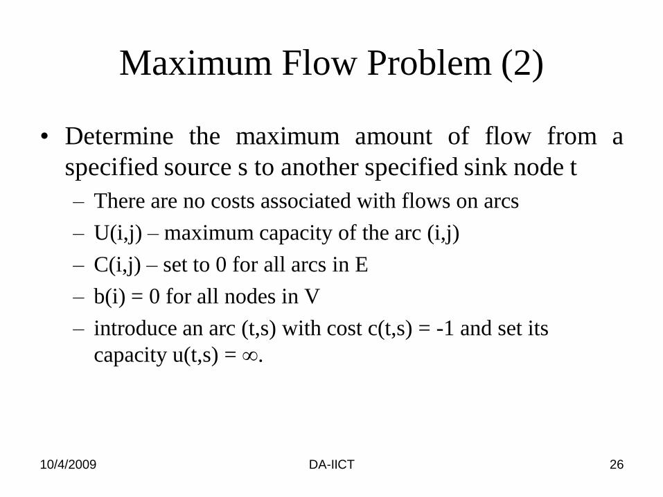
Maximum Flow Problem (2)

• Determine the maximum amount of flow from a

specified source s to another specified sink node t

– There are no costs associated with flows on arcs

– U(i,j) – maximum capacity of the arc (i,j)

– C(i,j) – set to 0 for all arcs in E

– b(i) = 0 for all nodes in V

– introduce an arc (t,s) with cost c(t,s) = -1 and set its

capacity u(t,s) = ∞.

10/4/2009 DA-IICT 27

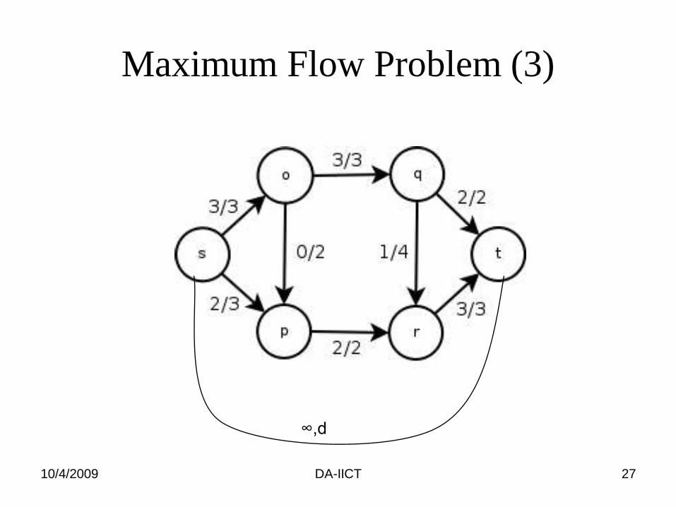
Maximum Flow Problem (3)

∞,d

10/4/2009 DA-IICT 28

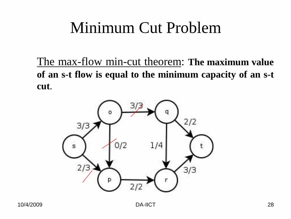
Minimum Cut Problem

The max-flow min-cut theorem: The maximum value

of an s-t flow is equal to the minimum capacity of an s-t

cut.

10/4/2009 DA-IICT 29

Assignment Problem

• Given two sets N1 and N2, a collection of pairs A in

N1 X N2 representing possible assignments, and a

cost c(i,j) associated with each arc (i, j), find a

minimum cost assignment.

– G = (N1UN2,A)

– B(i) = 1 for all i in N1 and b(i)=-1 for all i in N2

– U(i,j) = 1 for all (i,j) in A

10/4/2009 DA-IICT 30

Assignment Problem

A

CB

D

Assignment of Bandwidth to nodes to balance load

10/4/2009 DA-IICT 31

Restricted Assignment Problem

Assignment of Channels to nodes to maximize throughput

A 1

B

C

D

E

F

2

3

4

5

6

Channels Nodes

10/4/2009 DA-IICT 32

Generalized Flow Problem

• A generalization of minimum cost flow problem

• If x(i,j) units enter an arc (i,j) then σ(x(i,j)) units

arrive at node j, where for

– 0 < σ(x(i,j)) <= 1 it is a lossy network

– σ(x(i,j)) > 1 it a gainful network

10/4/2009 DA-IICT 33

Minimum Spanning Tree Problem (1)

An Example of a minimum spanning Tree

10/4/2009 DA-IICT 34

Minimum Spanning Tree Problem (2)

• A spanning Tree is a tree than spans all the nodes of

an undirected network.

• The cost of the spanning tree is the sum of the costs

(lengths) of its arcs.

• In the spanning tree problem, we need to determine a

spanning tree of minimum cost (or length).

10/4/2009 DA-IICT 35

Steiner Tree Problem (1)

• Steiner Tree problem: Given a set V of points

(vertices), interconnect them by a network of shortest

length, where the length is the sum of the lengths of

all edges.

• The difference between the Steiner tree problem and

the minimum spanning tree problem is that, in the

Steiner tree problem, extra intermediate vertices and

edges may be added to the graph in order to reduce

the length of the spanning tree.

10/4/2009 DA-IICT 36

Steiner Tree Problem (2)

Steiner Tree for 3 points Steiner Tree for 4 points

10/4/2009 DA-IICT 37

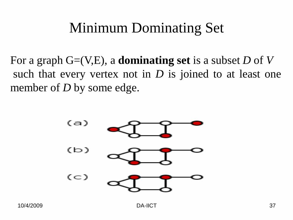
Minimum Dominating Set

For a graph G=(V,E), a dominating set is a subset D of V

such that every vertex not in D is joined to at least one

member of D by some edge.

10/4/2009 DA-IICT 38

l

Cost

Congestion Pricing Model

• Consider a resource of capacity C of which a fractionL has been consumed.

• The cost of the resource increases steeply as Lapproaches C (i.e. when the resource becomes abottleneck)

10/4/2009 DA-IICT 39

Virtual Circuit Routing

Given a graph G = (V,E), a sequence of routing

requests select a system of

paths between and of bandwidth λi for each

request so that the congestion (i.e. maximum load

on any edge) is minimized

10/4/2009 DA-IICT 40

Position Based Routing in Dynamic

Networks

A Unit Disk Graph Representation of an Ad hoc Network

10/4/2009 DA-IICT 41

Position Based Routing in Dynamic

Networks

• Each node knows its position relative to its one hop neighbors

in order to route packets

• Packets need to be forwarded in the geographical direction of

the destination based on local information

• State changes and node movement can cause frequent changes

in topology

• Not necessary to share state information globally since routing

decisions can be done in a greedy manner based on only local

information

• Routing decisions can be distributed and system will be

scalable as long it is loop free.

10/4/2009 DA-IICT 42

References

1. NETWORK FLOWS Theory, Algorithms, and Applications by RAVINDRA K.AHUJA, Prentice Hall.

2. Quality of service for Mobile ad-hoc networks by Shakeel Ahmed, Devi AhilyaVishwa Vidyalaya, Indore (M.P.), 2009.

3. Internet Algorithms: Design and Analysis by Alex Kesselman, MPI, Mini Course,2004.

4. OR Notes by J.E. Beaseley, http://people.brunel.ac.uk/~mastjjb/jeb/jeb.html.

5. Energy aware routing by Eero Nevalainen, 2003.

6. A Practical Algorithm for Constructing Oblivious Routing Schemes, by MarcinBieńkowski, Mirosław Korzeniowski and Harald Räcke.

7. Position based routing by Lili Zhang,www.cs.helsinki.fi/u/floreen/adhoc/zhang_slides.pdf .

8. Images were obtained from the following web sites

1. http://developer.symbian.com/

2. http://www.ee.surrey.ac.uk/

3. http://www.timboucher.com/

4. http://en.wikipedia.org/

5. http://www.ee.surrey.ac.uk/

6. http://compnetworking.about.com/