mathematical model for prediction and optimization of weld
TRANSCRIPT

metals
Article
Mathematical Model for Prediction and Optimizationof Weld Bead Geometry in All-Position AutomaticWelding of Pipes
Baoyi Liao 1,2, Yonghua Shi 1,2,* , Yanxin Cui 1,2, Shuwan Cui 1,2, Zexin Jiang 3 and Yaoyong Yi 4
1 School of Mechanical and Automotive Engineering, South China University of Technology,Guangzhou 510640, China; [email protected] (B.L.); [email protected] (Y.C.);[email protected] (S.C.)
2 Guangdong Provincial Engineering Research Center for Special Welding Technology and Equipment,South China University of Technology, Guangzhou 510640, China
3 Guangzhou Shipyard International Company Limited, Guangzhou 511462, China; [email protected] Guangdong Welding Institute (China-Ukraine E. O. Paton Institute of Welding), Guangzhou 510650, China;
[email protected]* Correspondence: [email protected]; Tel./Fax.: +86-208-7114-407
Received: 3 September 2018; Accepted: 21 September 2018; Published: 25 September 2018�����������������
Abstract: In this study all-position automatic tungsten inert gas (TIG) welding was exploited toenhance quality and efficiency in the welding of copper-nickel alloy pipes. The mathematical modelsof all-position automatic TIG weld bead shapes were conducted by the response surface method(RSM) on the foundation of central composition design (CCD). The statistical models were verifiedfor their significance and adequacy by analysis of variance (ANOVA). In addition, the influencesof welding peak current, welding velocity, welding duty ratio, and welding position on weld beadgeometry were investigated. Finally, optimal welding parameters at the welding positions of 0◦ to180◦ were determined by using RSM.
Keywords: all-position automatic tungsten inert gas (TIG) welding; optimal welding parameters;response surface method (RSM); lap joint; weld bead geometry
1. Introduction
With the fast development of heavy industries, all-position automatic tungsten inert gas (TIG)welding of pipes had been widely applied to industries such as shipbuilding, nuclear power, chemicalindustries, and natural gas transportation. Welding plays an important role in joining pipes [1].Traditional all-position welding of pipes is manual arc welding, but it has low welding efficiency,poor stability, and high cost. Moreover, the manual operation of pipe welding is a challenge to thewelder. In order to overcome the aforementioned shortcomings of manual arc welding, an all-positionautomatic TIG welding process has been developed in recent years. At present, there are four typesof automatic TIG butt-welding equipment for pipelines: closed welding heads, open welding heads,orbital welding trolleys, and thick-walled narrow gap TIG welding heads.
In all-position automatic TIG welding of pipes, especially for vertical and overhead positionwelding, it is a challenge to control the liquid metal flow down from the molten pool under theaction of gravity. Therefore, there is a need to adjust welding parameters to keep the droplettransition smooth. In order to obtain high-quality weld beads, selecting optimal weld parametersand controlling the weld bead profile are important. As is well known, weld bead shape has anoteworthy influence on the mechanical properties of lap joints. In all-position automatic TIG weldingof pipes, the weld bead profile is impacted not only by the weld parameters such as weld background
Metals 2018, 8, 756; doi:10.3390/met8100756 www.mdpi.com/journal/metals

Metals 2018, 8, 756 2 of 16
current, weld peak current, weld speed, weld voltage, but also by the welding position. Therefore,it is hard to obtain several optimal parameters to receive perfect weld bead profiles. To realizethis goal, the connection between weld parameters and weld bead shapes need to be established.A lot of research has been undertaken to establish mathematical models to optimize parametersand obtain the relationship [2,3]. Xu et al. [4] optimized the narrow gap all-position gas metal arc(GMA) welding parameters by employing the response surface method (RSM) and building regressionmodels to predict the parameters of weld bead geometry. Rao et al. [5] had obtained the influenceof welding parameters and statistical models for the prediction of weld bead shapes in pulsed GMAwelding. Koleva [6] researched the connection with electron beam welding parameters and weldbead geometry; moreover, the mathematical model can optimize welding parameters. Karthikeyanand Balasubramanian used RSM to optimize friction stir spot welding procedure parameters and toobtain maximum lap shear strength of the lap joint [7]. The statistical model was built at an invariableposition in inchoate research. However, in all-position automatic TIG welding of pipes, the weldingposition should be used as the input parameter of the statistical model because the weld includes flat,vertical and overhead positions [8], and welding position impacts the weld bead profile.
RSM can be used to predict the weld bead shape and mechanical properties in the weldingprocess [9–12]. The ultimate goal of this paper is to build a new all-position automatic TIG pipes’welding procedure and a mathematical model of weld bead geometry using RSM.
2. Materials and Methods
The schematic diagram of the system for all-position automatic TIG welding of pipelines is shownin Figure 1. The system includes an iOrbital 5000 welding machine, a TOA77 welding torch, a controlpanel, two argon tanks, a welding fixture and a cool water circulation system. The welding processwas as follows:
(1) Fixing the pipes with a welding fixture.(2) Inputting the cool water and argon gas into the TOA77 welding torch.(3) The protective gas was inputted into the pipes.(4) The welding torch weld around the pipes.
Metals 2018, 8, x FOR PEER REVIEW 2 of 16
weld peak current, weld speed, weld voltage, but also by the welding position. Therefore, it is hard
to obtain several optimal parameters to receive perfect weld bead profiles. To realize this goal, the
connection between weld parameters and weld bead shapes need to be established. A lot of research
has been undertaken to establish mathematical models to optimize parameters and obtain the
relationship [2,3]. Xu et al. [4] optimized the narrow gap all-position gas metal arc (GMA) welding
parameters by employing the response surface method (RSM) and building regression models to
predict the parameters of weld bead geometry. Rao et al. [5] had obtained the influence of welding
parameters and statistical models for the prediction of weld bead shapes in pulsed GMA welding.
Koleva [6] researched the connection with electron beam welding parameters and weld bead
geometry; moreover, the mathematical model can optimize welding parameters. Karthikeyan and
Balasubramanian used RSM to optimize friction stir spot welding procedure parameters and to
obtain maximum lap shear strength of the lap joint [7]. The statistical model was built at an invariable
position in inchoate research. However, in all-position automatic TIG welding of pipes, the welding
position should be used as the input parameter of the statistical model because the weld includes flat,
vertical and overhead positions [8], and welding position impacts the weld bead profile.
RSM can be used to predict the weld bead shape and mechanical properties in the welding
process [9–12]. The ultimate goal of this paper is to build a new all-position automatic TIG pipes’
welding procedure and a mathematical model of weld bead geometry using RSM.
2. Materials and Methods
The schematic diagram of the system for all-position automatic TIG welding of pipelines is
shown in Figure 1. The system includes an iOrbital 5000 welding machine, a TOA77 welding torch,
a control panel, two argon tanks, a welding fixture and a cool water circulation system. The welding
process was as follows:
(1) Fixing the pipes with a welding fixture.
(2) Inputting the cool water and argon gas into the TOA77 welding torch.
(3) The protective gas was inputted into the pipes.
(4) The welding torch weld around the pipes.
Interface
Cooling water
Argon Gas
Argon Gas
Welding direction
Handle
Welding power source
Torch
Weld seam
Pipe
Figure 1. The schematic diagram of the system for all-position automatic tungsten inert gas (TIG)
welding of pipes.
The workpieces used in this study are UNS (Unified Numbering System for Metas and Alloys)
C70600 with dimensions of Φ57 mm × 300 mm × 2 mm, but there is a flaring end of the pipe and the
diameter is 62 mm, as shown in Figure 2. The chemical compositions of the parent metal are listed in
Table 1. In this study, experiments were executed with one-sided welding with double-sided shaping
without an opening groove and welding wire, because the experiments melt the parent metal as filler
Figure 1. The schematic diagram of the system for all-position automatic tungsten inert gas (TIG)welding of pipes.
The workpieces used in this study are UNS (Unified Numbering System for Metas and Alloys)C70600 with dimensions of Φ57 mm × 300 mm × 2 mm, but there is a flaring end of the pipe and
Metals 2018, 8, 756 3 of 16
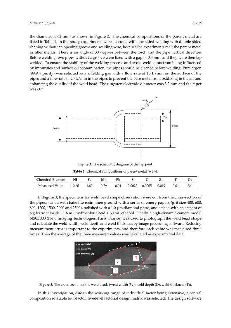
the diameter is 62 mm, as shown in Figure 2. The chemical compositions of the parent metal arelisted in Table 1. In this study, experiments were executed with one-sided welding with double-sidedshaping without an opening groove and welding wire, because the experiments melt the parent metalas filler metals. There is an angle of 30 degrees between the torch and the pipe vertical direction.Before welding, two pipes without a groove were fixed with a gap of 0.5 mm, and they were then lapwelded. To ensure the stability of the welding process and avoid weld joints from being influencedby impurities and surface oil contamination, the pipes should be cleaned before welding. Pure argon(99.9% purity) was selected as a shielding gas with a flow rate of 15 L/min on the surface of thepipes and a flow rate of 20 L/min in the pipes to prevent the base metal from oxidizing in the air andenhancing the quality of the weld bead. The tungsten electrode diameter was 3.2 mm and the taperwas 60◦.
Metals 2018, 8, x FOR PEER REVIEW 3 of 16
metals. There is an angle of 30 degrees between the torch and the pipe vertical direction. Before
welding, two pipes without a groove were fixed with a gap of 0.5 mm, and they were then lap welded.
To ensure the stability of the welding process and avoid weld joints from being influenced by
impurities and surface oil contamination, the pipes should be cleaned before welding. Pure argon
(99.9% purity) was selected as a shielding gas with a flow rate of 15 L/min on the surface of the pipes
and a flow rate of 20 L/min in the pipes to prevent the base metal from oxidizing in the air and
enhancing the quality of the weld bead. The tungsten electrode diameter was 3.2 mm and the taper
was 60°.
30°
62mm
2mm
57mm
Figure 2. The schematic diagram of the lap joint.
Table 1. Chemical compositions of parent metal (wt%).
Chemical
Element Ni Fe Mn Pb S C Zn P Cu
Measured Value 10.66 1.60 0.79 0.01 0.0023 0.0065 0.019 0.01 Bal
In Figure 3, the specimens for weld bead shape observation were cut from the cross-section of
the pipes, sealed with bake lite resin, then ground with a series of emery papers (grit size 400, 600,
800, 1200, 1500, 2000 and 2500), polished with a 1.0-μm diamond paste, and etched with an etchant
of 5 g ferric chloride + 16 mL hydrochloric acid + 60 mL ethanol. Finally, a high-dynamic camera
model NSC1003 (New Imaging Technologies, Paris, France) was used to photograph the weld bead
shape and calculate the weld width, weld depth and weld thickness by image processing software.
Reducing measurement error is important to the experiments, and therefore each value was
measured three times. Then the average of the three measured values was calculated as experimental
data.
In this investigation, due to the working range of individual factor being extensive, a central
composition rotatable four-factor, five-level factorial design matrix was selected. The design software
Design-Expert (V 10. 0. 7, Stat-Ease, MN, USA) was used to establish the design matrix and process
the experimental data.
The steps of this investigation are as follows:
(a) Validation of the primary factors;
(b) Confirming the working range of the control variables;
(c) Establishing trial matrix by Design-Expert V10.0.7 software;
(d) Conducting the experiments as per the design matrix;
(e) Recording the response parameters;
(f) Building statistical models;
(g) Calculating regression coefficients of the multinomial;
Figure 2. The schematic diagram of the lap joint.
Table 1. Chemical compositions of parent metal (wt%).
Chemical Element Ni Fe Mn Pb S C Zn P Cu
Measured Value 10.66 1.60 0.79 0.01 0.0023 0.0065 0.019 0.01 Bal
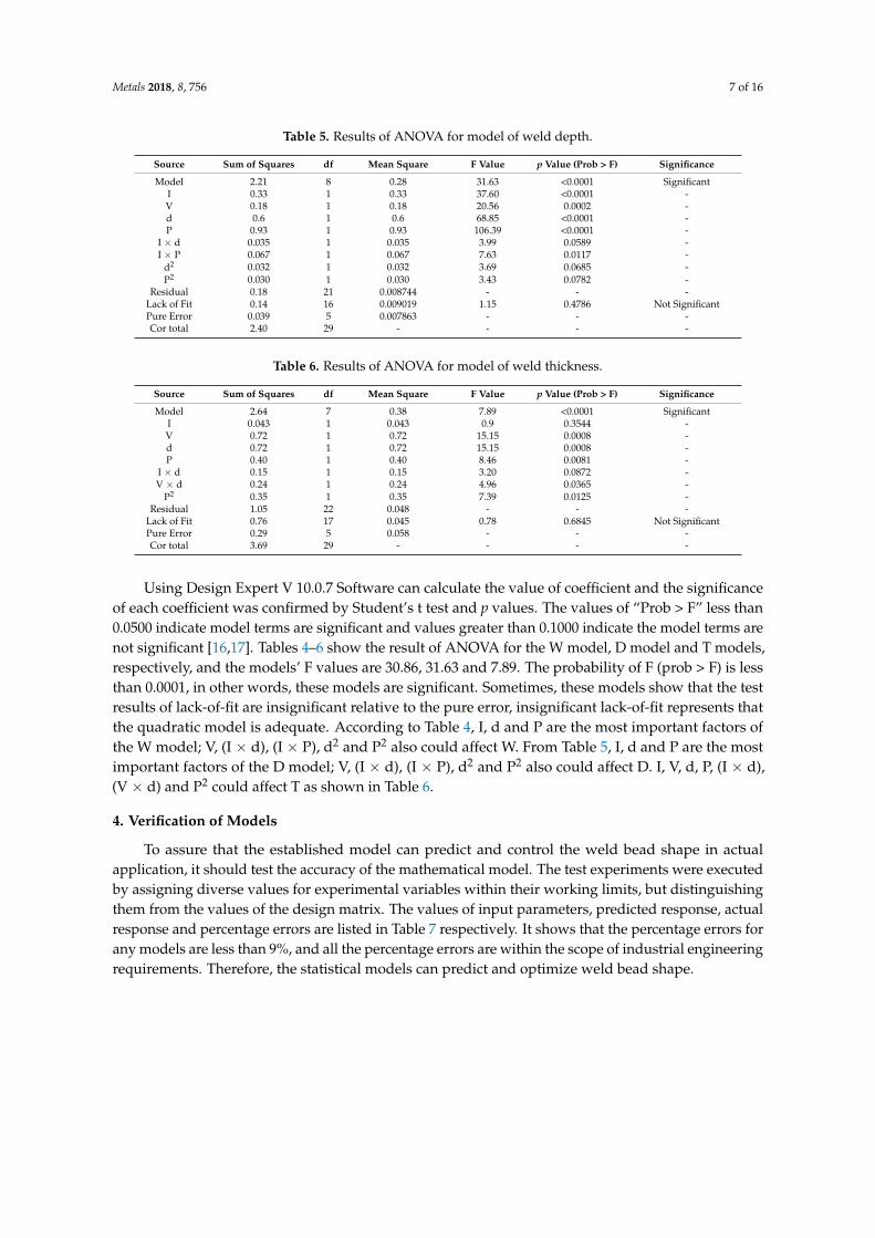
In Figure 3, the specimens for weld bead shape observation were cut from the cross-section ofthe pipes, sealed with bake lite resin, then ground with a series of emery papers (grit size 400, 600,800, 1200, 1500, 2000 and 2500), polished with a 1.0-µm diamond paste, and etched with an etchant of5 g ferric chloride + 16 mL hydrochloric acid + 60 mL ethanol. Finally, a high-dynamic camera modelNSC1003 (New Imaging Technologies, Paris, France) was used to photograph the weld bead shapeand calculate the weld width, weld depth and weld thickness by image processing software. Reducingmeasurement error is important to the experiments, and therefore each value was measured threetimes. Then the average of the three measured values was calculated as experimental data.
Metals 2018, 8, x FOR PEER REVIEW 4 of 16
(h) Checking the adequacy of the statistical model;
(i) Verification of models;
(j) Receiving, finally, the statistical model;
(k) Analysis of results;
(l) Optimizing welding parameters.
3. Creating Mathematical Model
Based on the initial experimental results, four very important welding parameters affecting the
weld bead geometry are the welding peak current (I), welding velocity (V), welding duty ratio (d)
and welding position (P). The duty ratio is the ratio of welding peak current time to the pulse period.
In order to create a mathematical model to describe and forecast the weld bead geometry in all-
position automatic welding, I, V, d, and P were chosen as input parameters. The schematic diagrams
of the weld bead shape and welding position are shown in Figures 3 and 4, respectively.
Figure 3. The cross-section of the weld bead. (weld width (W), weld depth (D), weld thickness (T)).
Figure 4. Schematic diagram of welding position.
Before this experiment, the control variable method was used to find out the working range of
input parameters. The working range was determined by the steady welding procedure and invisible
weld defects. In order to obtain optimized welding parameters, the establishment of a test parameter
matrix adopts the center composed design (CCD) in the regression design method. In the CCD
design, the upper and lower limit values of the input parameters were coded as ± β, the value of β is
dependent on the number of input parameters and β = 1/4(2 )k , k is the number of input parameters.
The upper level and lower level were coded as ±1 respectively and the center point was coded as 0.
In this research, there are 4 input parameters, so β is 2. Therefore, the upper and lower limit values
of the input parameters were coded as ±2. The codes values for intermediate levels can be calculated
by Equation (1):
X𝑖 = 2[2𝑋 − (𝑋𝑚𝑎𝑥 + 𝑋𝑚𝑖𝑛)]/[𝑋𝑚𝑎𝑥 − 𝑋𝑚𝑖𝑛] (1)
Figure 3. The cross-section of the weld bead. (weld width (W), weld depth (D), weld thickness (T)).
In this investigation, due to the working range of individual factor being extensive, a centralcomposition rotatable four-factor, five-level factorial design matrix was selected. The design software

Metals 2018, 8, 756 4 of 16
Design-Expert (V 10. 0. 7, Stat-Ease, MN, USA) was used to establish the design matrix and processthe experimental data.
The steps of this investigation are as follows:
(a) Validation of the primary factors;(b) Confirming the working range of the control variables;(c) Establishing trial matrix by Design-Expert V10.0.7 software;(d) Conducting the experiments as per the design matrix;(e) Recording the response parameters;(f) Building statistical models;(g) Calculating regression coefficients of the multinomial;(h) Checking the adequacy of the statistical model;(i) Verification of models;(j) Receiving, finally, the statistical model;(k) Analysis of results;(l) Optimizing welding parameters.
3. Creating Mathematical Model
Based on the initial experimental results, four very important welding parameters affecting theweld bead geometry are the welding peak current (I), welding velocity (V), welding duty ratio (d)and welding position (P). The duty ratio is the ratio of welding peak current time to the pulse period.In order to create a mathematical model to describe and forecast the weld bead geometry in all-positionautomatic welding, I, V, d, and P were chosen as input parameters. The schematic diagrams of theweld bead shape and welding position are shown in Figures 3 and 4, respectively.
Metals 2018, 8, x FOR PEER REVIEW 4 of 16
(h) Checking the adequacy of the statistical model;
(i) Verification of models;
(j) Receiving, finally, the statistical model;
(k) Analysis of results;
(l) Optimizing welding parameters.
3. Creating Mathematical Model
Based on the initial experimental results, four very important welding parameters affecting the
weld bead geometry are the welding peak current (I), welding velocity (V), welding duty ratio (d)
and welding position (P). The duty ratio is the ratio of welding peak current time to the pulse period.
In order to create a mathematical model to describe and forecast the weld bead geometry in all-
position automatic welding, I, V, d, and P were chosen as input parameters. The schematic diagrams
of the weld bead shape and welding position are shown in Figures 3 and 4, respectively.
Figure 3. The cross-section of the weld bead. (weld width (W), weld depth (D), weld thickness (T)).
Figure 4. Schematic diagram of welding position.
Before this experiment, the control variable method was used to find out the working range of
input parameters. The working range was determined by the steady welding procedure and invisible
weld defects. In order to obtain optimized welding parameters, the establishment of a test parameter
matrix adopts the center composed design (CCD) in the regression design method. In the CCD
design, the upper and lower limit values of the input parameters were coded as ± β, the value of β is
dependent on the number of input parameters and β = 1/4(2 )k , k is the number of input parameters.
The upper level and lower level were coded as ±1 respectively and the center point was coded as 0.
In this research, there are 4 input parameters, so β is 2. Therefore, the upper and lower limit values
of the input parameters were coded as ±2. The codes values for intermediate levels can be calculated
by Equation (1):
X𝑖 = 2[2𝑋 − (𝑋𝑚𝑎𝑥 + 𝑋𝑚𝑖𝑛)]/[𝑋𝑚𝑎𝑥 − 𝑋𝑚𝑖𝑛] (1)
Figure 4. Schematic diagram of welding position.
Before this experiment, the control variable method was used to find out the working range ofinput parameters. The working range was determined by the steady welding procedure and invisibleweld defects. In order to obtain optimized welding parameters, the establishment of a test parametermatrix adopts the center composed design (CCD) in the regression design method. In the CCDdesign, the upper and lower limit values of the input parameters were coded as ± β, the value of β is
dependent on the number of input parameters and β = (2k)1/4
, k is the number of input parameters.The upper level and lower level were coded as ±1 respectively and the center point was coded as 0.In this research, there are 4 input parameters, so β is 2. Therefore, the upper and lower limit values ofthe input parameters were coded as ±2. The codes values for intermediate levels can be calculated byEquation (1):
Xi = 2[2X − (Xmax + Xmin)]/[Xmax − Xmin] (1)

Metals 2018, 8, 756 5 of 16
In Equation (1), Xi is the desired code value of a variable X, and range of values of X is from Xminto Xmax; Xmax is the upper limits and Xmin is lower limits of the variable X [13,14].
The factor levels and coded values have been listed in Table 2. The experimental design matrix(Table 3) includes 30 sets of coded situations and constitutes a full replication four-factor factorialdesign of 16 points, 8 star points and 6 center points [7].
Table 2. Important weld parameters and their levels for copper–nickel alloy pipe.
Factors UnitCoded Value
−2 −1 0 1 2
I A 114 117 120 123 126V mm/min 57 60 63 66 69d % 40 45 50 55 60P ◦ 0 45 90 135 180
Table 3. Trial design matrix and response of copper–nickel alloy lap joints.
Std RunCoded Variables Response Parameters
I (A) V (mm/min) D (%) P (degree) W (mm) D (mm) T (mm)
1 7 117 60 45 45 1.416 0.29 1.9782 10 123 60 45 45 1.615 0.363 2.1423 6 117 66 45 45 1.016 0.199 1.7974 19 123 66 45 45 1.325 0.272 1.895 11 117 60 55 45 2.877 0.577 2.5416 24 123 60 55 45 4.2 0.851 2.7517 22 117 66 55 45 1.575 0.315 1.9958 26 123 66 55 45 2.373 0.462 2.2329 29 117 60 45 135 3.255 0.637 2.18510 30 123 60 45 135 4.956 1.02 2.31411 14 117 66 45 135 2.583 0.525 1.93212 8 123 66 45 135 3.591 0.706 2.7313 5 117 60 55 135 4.074 0.835 3.02414 23 123 60 55 135 5.796 1.298 2.54115 16 117 66 55 135 3.297 0.606 2.37916 15 123 66 55 135 5.754 1.179 2.03417 12 114 63 50 90 2.268 0.441 2.33118 28 126 63 50 90 3.717 0.762 2.43619 20 120 57 50 90 3.402 0.697 2.66720 9 120 69 50 90 2.856 0.462 1.82721 27 120 63 40 90 2.226 0.356 1.65922 4 120 63 60 90 5.859 1.201 2.47823 13 120 63 50 0 0.987 0.202 1.53324 17 120 63 50 180 4.032 0.826 2.18425 3 120 63 50 90 3.412 0.699 2.33126 2 120 63 50 90 3.533 0.724 2.82627 25 120 63 50 90 3.641 0.528 2.46128 21 120 63 50 90 2.755 0.597 2.09829 1 120 63 50 90 2.562 0.74 2.35630 18 120 63 50 90 2.878 0.742 2.501
In order to better reflect the weld bead geometry, reasonable response parameters need to beselected. The response parameters were named weld width (W), weld depth (D), and weld thickness(T). Figure 3 shows the cross section of weld bead.
On the foundation of central composite design matrix, the value of input parameters, responseparameters and the regression model can be built. The connection between measured response and theinput parameters could be shown as y = f (x1, x2, . . . , xi) + ε, where y is the value of measured response,xi is the value of the input parameter, and ε is the systematic error. Y is a power transformation ofy [11,15], so the second-order polynomial can be expressed as Equation (2):
Y = b0 + ∑4i=1 bixi + ∑3
i=1 ∑4j=i+1 bijxiyj + ∑4
i=1 biixi2 (2)

Metals 2018, 8, 756 6 of 16
where, b0 is the average of the measured response, the regression coefficients such as bi, bij and biidepend on linear, interaction and squared terms of factors, respectively.
Almost all response surface method problems can be approximated by these polynomials, andthe regression coefficients could be obtained by the least squares method.
The regression model adopts the method of stepwise regression. Firstly, the regression modeleliminates the insignificant terms and calculates the regression coefficients until the significant termsand the lack-of-fit terms of the regression model meet the requirements of the regression model. Finally,the relational expressions about all-position automatic TIG welding of the pipe within the range of0–180◦ were obtained as Equations (3)–(8), which show the relationship between weld geometry shapeand input parameters.
The final equations in terms of coded factors are given as follows:
W = 3.07 + 0.52 I − 0.32 V + 0.73 d + 0.96 P + 0.19 I × d + 0.27 I × P + 0.22 d2 − 0.16 P2 (3)
D = 0.64 + 0.12 I − 0.087 V + 0.16 d + 0.20 P + 0.047 I × d + 0.065 I × P + 0.034 d2 − 0.032 P2 (4)
T = 2.36 + 0.042 I − 0.17 V + 0.17 d + 0.13 P − 0.098 I × d − 0.12 V × d − 0.11 P2 (5)
The final equations in terms of actual factors are given as follows:
W = 100.19346 − 0.64732 I − 0.10788 V − 2.29476 d − 0.20122 P +0.012846 I × d + 0.00197176 I × P + 0.00898719 d2 − 0.000783063 P2 (6)
D = 22.87088 − 0.15965 I − 0.028847 V − 0.47648 d − 0.050128 P +0.00311250 I × d + 0.000478241 I × P + 0.00134656 d2 − 0.0000160301 P2 (7)
T = −62.80003 + 0.34011 I + 0.34775 V + 1.32831 d + 0.012728 P− 0.00652083 I × d − 0.00811250 V × d − 0.0000546879 P2 (8)
Analysis of variance (ANOVA) was used to determine the significance and suitability of theregression model. Tables 4–6 show the ANOVA analysis of the weld width, the weld depth and theweld thickness model respectively.
Table 4. Results of analysis of variance (ANOVA) for model of weld width.
Source Sum of Squares df * Mean Square F Value p Value (Prob > F) Significance
Model 47.8 8 5.98 30.86 <0.0001 SignificantI 6.42 1 6.42 33.17 <0.0001 -V 2.51 1 2.51 12.98 0.0017 -d 12.69 1 12.69 65.56 <0.0001 -P 22.04 1 22.04 113.82 <0.0001 -
I × d 0.59 1 0.59 3.07 0.0945 -I × P 1.13 1 1.13 5.85 0.0247 -
d2 1.44 1 1.44 7.42 0.0127 -P2 0.72 1 0.72 3.69 0.0683 -
Residual 4.07 21 0.19 - - -Lack of Fit 3.04 16 0.19 0.92 0.5944 Not SignificantPure Error 1.03 5 0.21 - - -Cor total 51.87 29 - - - -
* Degree of freedom (df), a concept in statics, indicates the number of unconstrained variables in calculating astatistical magnitude. According to the usual definition, df = n − k, n is the number of samples and k is the numberof constrained variables or conditional number, while k is also the quantity of the other independent statisticalmagnitude in calculating one statistical magnitude.
Metals 2018, 8, 756 7 of 16
Table 5. Results of ANOVA for model of weld depth.
Source Sum of Squares df Mean Square F Value p Value (Prob > F) Significance
Model 2.21 8 0.28 31.63 <0.0001 SignificantI 0.33 1 0.33 37.60 <0.0001 -V 0.18 1 0.18 20.56 0.0002 -d 0.6 1 0.6 68.85 <0.0001 -P 0.93 1 0.93 106.39 <0.0001 -
I × d 0.035 1 0.035 3.99 0.0589 -I × P 0.067 1 0.067 7.63 0.0117 -
d2 0.032 1 0.032 3.69 0.0685 -P2 0.030 1 0.030 3.43 0.0782 -
Residual 0.18 21 0.008744 - - -Lack of Fit 0.14 16 0.009019 1.15 0.4786 Not SignificantPure Error 0.039 5 0.007863 - - -Cor total 2.40 29 - - - -
Table 6. Results of ANOVA for model of weld thickness.
Source Sum of Squares df Mean Square F Value p Value (Prob > F) Significance
Model 2.64 7 0.38 7.89 <0.0001 SignificantI 0.043 1 0.043 0.9 0.3544 -V 0.72 1 0.72 15.15 0.0008 -d 0.72 1 0.72 15.15 0.0008 -P 0.40 1 0.40 8.46 0.0081 -
I × d 0.15 1 0.15 3.20 0.0872 -V × d 0.24 1 0.24 4.96 0.0365 -
P2 0.35 1 0.35 7.39 0.0125 -Residual 1.05 22 0.048 - - -
Lack of Fit 0.76 17 0.045 0.78 0.6845 Not SignificantPure Error 0.29 5 0.058 - - -Cor total 3.69 29 - - - -
Using Design Expert V 10.0.7 Software can calculate the value of coefficient and the significanceof each coefficient was confirmed by Student’s t test and p values. The values of “Prob > F” less than0.0500 indicate model terms are significant and values greater than 0.1000 indicate the model terms arenot significant [16,17]. Tables 4–6 show the result of ANOVA for the W model, D model and T models,respectively, and the models’ F values are 30.86, 31.63 and 7.89. The probability of F (prob > F) is lessthan 0.0001, in other words, these models are significant. Sometimes, these models show that the testresults of lack-of-fit are insignificant relative to the pure error, insignificant lack-of-fit represents thatthe quadratic model is adequate. According to Table 4, I, d and P are the most important factors ofthe W model; V, (I × d), (I × P), d2 and P2 also could affect W. From Table 5, I, d and P are the mostimportant factors of the D model; V, (I × d), (I × P), d2 and P2 also could affect D. I, V, d, P, (I × d),(V × d) and P2 could affect T as shown in Table 6.
4. Verification of Models
To assure that the established model can predict and control the weld bead shape in actualapplication, it should test the accuracy of the mathematical model. The test experiments were executedby assigning diverse values for experimental variables within their working limits, but distinguishingthem from the values of the design matrix. The values of input parameters, predicted response, actualresponse and percentage errors are listed in Table 7 respectively. It shows that the percentage errors forany models are less than 9%, and all the percentage errors are within the scope of industrial engineeringrequirements. Therefore, the statistical models can predict and optimize weld bead shape.

Metals 2018, 8, 756 8 of 16
Table 7. Predicted values and actual values of the weld bead geometry.
Designation Run 1 2 3 4 5
InputParameters
I (A) 123 122 119 117 115V (mm/min) 60 60 60 62 63
d (%) 55 45 40 60 55P (degree) 0 45 90 135 180
PredictedValues
W (mm) 1.977 1.818 2.788 3.958 4.067D (mm) 0.426 0.372 0.574 0.783 0.799T (mm) 2.071 2.091 2.194 2.707 2.406
ActualValues
W (mm) 1.839 1.978 2.581 3.615 4.256T (mm) 0.346 0.346 0.596 0.759 0.954W (mm) 2.204 1.991 2.345 2.891 2.278
PercentageError ** (%)
W −6.98 8.8 −7.43 −8.67 4.65D −7.04 −6.99 3.38 −4.29 6.88T 6.42 −4.78 7.03 6.8 −5.32
** Percentage error = actual value−predicted valuepredicted value × 100.
5. Results and Discussion
According to the all models, the prime and interaction influences of input weld parameters onweld bead geometry can be found.
5.1. Influences of Welding Peak Current on Weld Width (W), Weld Depth (D), and Weld Thickness (T)
Considering the influence of the single factor welding peak current on the weld bead geometry,it can be shown from Figure 5 that the welding peak current increases with the increase in weld width,weld depth and weld thickness. This is because with weld peak current increasing leads to heat inputincrease per unit time, which is good for the weld metal melted and enhancing the deposition efficiency.As the peak current increases, the weld width and depth increase significantly, while weld thicknessincreases less. The weld thickness increases gradually from 2.331 to 2.436 mm with the increase inwelding peak current from 114 to 126 A. This is because as the weld peak current increases, the arcforce also increases, and the liquid metal is blown to both sides of the molten pool under the action ofarc force, so the weld thickness increases indistinctly.
Metals 2018, 8, x FOR PEER REVIEW 8 of 16
executed by assigning diverse values for experimental variables within their working limits, but
distinguishing them from the values of the design matrix. The values of input parameters, predicted
response, actual response and percentage errors are listed in Table 7 respectively. It shows that the
percentage errors for any models are less than 9%, and all the percentage errors are within the scope
of industrial engineering requirements. Therefore, the statistical models can predict and optimize
weld bead shape.
Table 7. Predicted values and actual values of the weld bead geometry.
Designation Run 1 2 3 4 5
Input Parameters I (A) 123 122 119 117 115
V (mm/min) 60 60 60 62 63
d (%) 55 45 40 60 55
P (degree) 0 45 90 135 180
Predicted Values W (mm) 1.977 1.818 2.788 3.958 4.067
D (mm) 0.426 0.372 0.574 0.783 0.799
T (mm) 2.071 2.091 2.194 2.707 2.406
Actual Values W (mm) 1.839 1.978 2.581 3.615 4.256
T (mm) 0.346 0.346 0.596 0.759 0.954
W (mm) 2.204 1.991 2.345 2.891 2.278
Percentage Error
** (%)
W ‒6.98 8.8 ‒7.43 ‒8.67 4.65
D ‒7.04 ‒6.99 3.38 ‒4.29 6.88
T 6.42 ‒4.78 7.03 6.8 ‒5.32
** Percentage error = 𝒂𝒄𝒕𝒖𝒂𝒍 𝒗𝒂𝒍𝒖𝒆−𝒑𝒓𝒆𝒅𝒊𝒄𝒕𝒆𝒅 𝒗𝒂𝒍𝒖𝒆
𝒑𝒓𝒆𝒅𝒊𝒄𝒕𝒆𝒅 𝒗𝒂𝒍𝒖𝒆 × 100
5. Results and Discussion
According to the all models, the prime and interaction influences of input weld parameters on
weld bead geometry can be found.
5.1. Influences of Welding Peak Current on Weld Width (W), Weld Depth (D), and Weld Thickness (T)
Considering the influence of the single factor welding peak current on the weld bead geometry,
it can be shown from Figure 5 that the welding peak current increases with the increase in weld
width, weld depth and weld thickness. This is because with weld peak current increasing leads to
heat input increase per unit time, which is good for the weld metal melted and enhancing the
deposition efficiency. As the peak current increases, the weld width and depth increase significantly,
while weld thickness increases less. The weld thickness increases gradually from 2.331 to 2.436 mm
with the increase in welding peak current from 114 to 126 A. This is because as the weld peak current
increases, the arc force also increases, and the liquid metal is blown to both sides of the molten pool
under the action of arc force, so the weld thickness increases indistinctly.
111 114 117 120 123 126 129
0.0
0.5
1.0
1.5
2.0
2.5
3.0
3.5
4.0
Wel
d b
ead g
eom
etry
par
amet
er (
mm
)
Peak current (A)
Weld width (W)
Weld depth (D)
Weld thickness (T)
Figure 5. Influence of weld peak current on weld bead. (Welding velocity (V) = 63 mm/min, weldingduty ratio (d) = 50%, welding position (P) = 90◦).
Metals 2018, 8, 756 9 of 16
5.2. Influences of Weld Velocity on W, D and T
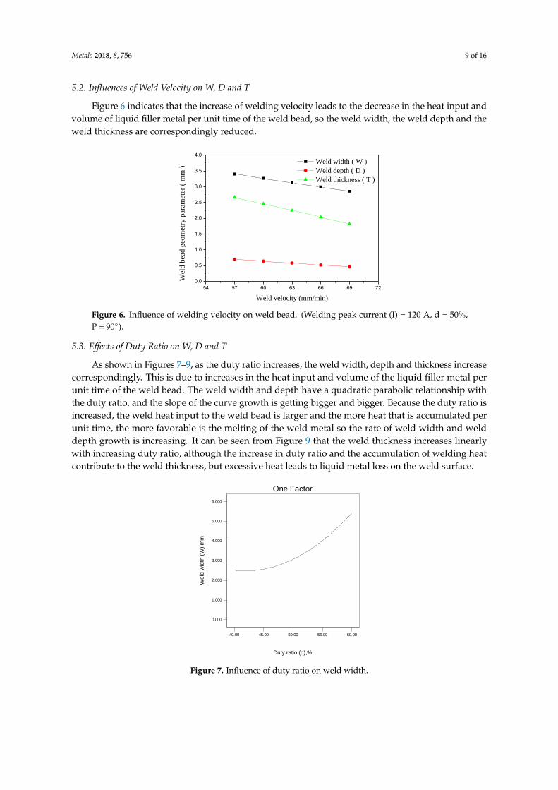
Figure 6 indicates that the increase of welding velocity leads to the decrease in the heat input andvolume of liquid filler metal per unit time of the weld bead, so the weld width, the weld depth and theweld thickness are correspondingly reduced.
Metals 2018, 8, x FOR PEER REVIEW 9 of 16
Figure 5. Influence of weld peak current on weld bead. (Welding velocity (V) = 63 mm/min, welding
duty ratio (d) = 50%, welding position (P) = 90°).
5.2. Influences of Weld Velocity on W, D and T
Figure 6 indicates that the increase of welding velocity leads to the decrease in the heat input
and volume of liquid filler metal per unit time of the weld bead, so the weld width, the weld depth
and the weld thickness are correspondingly reduced.
54 57 60 63 66 69 72
0.0
0.5
1.0
1.5
2.0
2.5
3.0
3.5
4.0
Weld width ( W )
Weld depth ( D )
Weld thickness ( T )
Wel
d b
ead
geo
met
ry p
aram
eter
( m
m )
Weld velocity (mm/min)
Figure 6. Influence of welding velocity on weld bead. (Welding peak current (I) = 120 A, d = 50%, P =
90°).
5.3. Effects of Duty Ratio on W, D and T
As shown in Figures 7–9, as the duty ratio increases, the weld width, depth and thickness
increase correspondingly. This is due to increases in the heat input and volume of the liquid filler
metal per unit time of the weld bead. The weld width and depth have a quadratic parabolic
relationship with the duty ratio, and the slope of the curve growth is getting bigger and bigger.
Because the duty ratio is increased, the weld heat input to the weld bead is larger and the more heat
that is accumulated per unit time, the more favorable is the melting of the weld metal so the rate of
weld width and weld depth growth is increasing. It can be seen from Figure 9 that the weld thickness
increases linearly with increasing duty ratio, although the increase in duty ratio and the accumulation
of welding heat contribute to the weld thickness, but excessive heat leads to liquid metal loss on the
weld surface.
Figure7. Influence of duty ratio on weld width.
Design-Expert?SoftwareFactor Coding: ActualW
X1 = C: d
Actual FactorsA: I = 120.00B: V = 63.00D: P = 90.00
Duty ratio (d),%
40.00 45.00 50.00 55.00 60.00
Weld
wid
th (
W),
mm
0.000
1.000
2.000
3.000
4.000
5.000
6.000
One Factor
Figure 6. Influence of welding velocity on weld bead. (Welding peak current (I) = 120 A, d = 50%,P = 90◦).
5.3. Effects of Duty Ratio on W, D and T
As shown in Figures 7–9, as the duty ratio increases, the weld width, depth and thickness increasecorrespondingly. This is due to increases in the heat input and volume of the liquid filler metal perunit time of the weld bead. The weld width and depth have a quadratic parabolic relationship withthe duty ratio, and the slope of the curve growth is getting bigger and bigger. Because the duty ratio isincreased, the weld heat input to the weld bead is larger and the more heat that is accumulated perunit time, the more favorable is the melting of the weld metal so the rate of weld width and welddepth growth is increasing. It can be seen from Figure 9 that the weld thickness increases linearlywith increasing duty ratio, although the increase in duty ratio and the accumulation of welding heatcontribute to the weld thickness, but excessive heat leads to liquid metal loss on the weld surface.
Metals 2018, 8, x FOR PEER REVIEW 9 of 16
Figure 5. Influence of weld peak current on weld bead. (Welding velocity (V) = 63 mm/min, welding
duty ratio (d) = 50%, welding position (P) = 90°).
5.2. Influences of Weld Velocity on W, D and T
Figure 6 indicates that the increase of welding velocity leads to the decrease in the heat input
and volume of liquid filler metal per unit time of the weld bead, so the weld width, the weld depth
and the weld thickness are correspondingly reduced.
54 57 60 63 66 69 72
0.0
0.5
1.0
1.5
2.0
2.5
3.0
3.5
4.0
Weld width ( W )
Weld depth ( D )
Weld thickness ( T )
Wel
d b
ead
geo
met
ry p
aram
eter
( m
m )
Weld velocity (mm/min)
Figure 6. Influence of welding velocity on weld bead. (Welding peak current (I) = 120 A, d = 50%, P =
90°).
5.3. Effects of Duty Ratio on W, D and T
As shown in Figures 7–9, as the duty ratio increases, the weld width, depth and thickness
increase correspondingly. This is due to increases in the heat input and volume of the liquid filler
metal per unit time of the weld bead. The weld width and depth have a quadratic parabolic
relationship with the duty ratio, and the slope of the curve growth is getting bigger and bigger.
Because the duty ratio is increased, the weld heat input to the weld bead is larger and the more heat
that is accumulated per unit time, the more favorable is the melting of the weld metal so the rate of
weld width and weld depth growth is increasing. It can be seen from Figure 9 that the weld thickness
increases linearly with increasing duty ratio, although the increase in duty ratio and the accumulation
of welding heat contribute to the weld thickness, but excessive heat leads to liquid metal loss on the
weld surface.
Figure7. Influence of duty ratio on weld width.
Design-Expert?SoftwareFactor Coding: ActualW
X1 = C: d
Actual FactorsA: I = 120.00B: V = 63.00D: P = 90.00
Duty ratio (d),%
40.00 45.00 50.00 55.00 60.00
Weld
wid
th (
W),
mm
0.000
1.000
2.000
3.000
4.000
5.000
6.000
One Factor
Figure 7. Influence of duty ratio on weld width.

Metals 2018, 8, 756 10 of 16Metals 2018, 8, x FOR PEER REVIEW 10 of 16
Figure 8. Influence of duty ratio on weld depth.
Figure 9. Influence of duty ratio on weld thickness.
5.4. Effects of Welding Position on W, D and T
As shown in Figures 10 and 11, as the degree of welding position increases, the weld width and
weld depth increase correspondingly in the welding interval of 0–180°. The weld width and weld
depth have a quadratic parabolic relationship to the degree of welding position, and the slope of the
curve is getting smaller and smaller due to the gravity of the molten pool and the flow of molten
metal along the weld bead during welding. Figure 12 shows the weld thickness increases first and
then decreases. The gravity of the molten pool at different welding positions was shown in Figure 13.
It was decomposed into a tangential force Gt and a radial force Gr. When welding in the 0–180°
interval, the molten pool is subjected to the tangential force Gt, which leads to the molten liquid metal
flowing down along the weld bead, and the flowing liquid metal can preheat the remaining weld
bead and fill the weld bead, so the shape parameters of the weld width, weld depth and the weld
thickness will increase with the increasing of the welding position degree. But when welding is in the
0–90°interval, the molten pool is subjected to the radial force Gr, and Gr = G cosθ. As the degree of
the welding position increases, the radial force becomes smaller and smaller, and the direction of the
radial force points to the center of the pipe; In the 90–180°interval welding, the molten pool is
subjected to the direction of the radial force back to the center of the pipe, and Gr = G sin(θ‒90); with
the welding position degree increasing, Gr becomes larger and larger, hindering the increase in weld
width, depth and thickness. Therefore, the slope of the curve growth is getting smaller and smaller.
Figure 12 shows the peak value of weld thickness for all values of P is received when P is 116°.
Design-Expert?Software
Factor Coding: Actual
D
X1 = C: d
Actual Factors
A: I = 120.00
B: V = 63.00
D: P = 90.00
40.00 44.00 48.00 52.00 56.00 60.00
Duty ratio (d),%
We
ld d
ep
th (
D),
mm
0.000
0.500
1.000
1.500
One Factor
Design-Expert?Software
Factor Coding: Actual
T
X1 = C: d
Actual Factors
A: I = 120.00
B: V = 63.00
D: P = 90.00
40.00 44.00 48.00 52.00 56.00 60.00
Duty ratio (d),%
We
ld th
ickn
ess (
T),
mm
0.000
0.500
1.000
1.500
2.000
2.500
3.000
One Factor
Figure 8. Influence of duty ratio on weld depth.
Metals 2018, 8, x FOR PEER REVIEW 10 of 16
Figure 8. Influence of duty ratio on weld depth.
Figure 9. Influence of duty ratio on weld thickness.
5.4. Effects of Welding Position on W, D and T
As shown in Figures 10 and 11, as the degree of welding position increases, the weld width and
weld depth increase correspondingly in the welding interval of 0–180°. The weld width and weld
depth have a quadratic parabolic relationship to the degree of welding position, and the slope of the
curve is getting smaller and smaller due to the gravity of the molten pool and the flow of molten
metal along the weld bead during welding. Figure 12 shows the weld thickness increases first and
then decreases. The gravity of the molten pool at different welding positions was shown in Figure 13.
It was decomposed into a tangential force Gt and a radial force Gr. When welding in the 0–180°
interval, the molten pool is subjected to the tangential force Gt, which leads to the molten liquid metal
flowing down along the weld bead, and the flowing liquid metal can preheat the remaining weld
bead and fill the weld bead, so the shape parameters of the weld width, weld depth and the weld
thickness will increase with the increasing of the welding position degree. But when welding is in the
0–90°interval, the molten pool is subjected to the radial force Gr, and Gr = G cosθ. As the degree of
the welding position increases, the radial force becomes smaller and smaller, and the direction of the
radial force points to the center of the pipe; In the 90–180°interval welding, the molten pool is
subjected to the direction of the radial force back to the center of the pipe, and Gr = G sin(θ‒90); with
the welding position degree increasing, Gr becomes larger and larger, hindering the increase in weld
width, depth and thickness. Therefore, the slope of the curve growth is getting smaller and smaller.
Figure 12 shows the peak value of weld thickness for all values of P is received when P is 116°.
Design-Expert?Software
Factor Coding: Actual
D
X1 = C: d
Actual Factors
A: I = 120.00
B: V = 63.00
D: P = 90.00
40.00 44.00 48.00 52.00 56.00 60.00
Duty ratio (d),%
We
ld d
ep
th (
D),
mm
0.000
0.500
1.000
1.500
One Factor
Design-Expert?Software
Factor Coding: Actual
T
X1 = C: d
Actual Factors
A: I = 120.00
B: V = 63.00
D: P = 90.00
40.00 44.00 48.00 52.00 56.00 60.00
Duty ratio (d),%
We
ld th
ickn
ess (
T),
mm
0.000
0.500
1.000
1.500
2.000
2.500
3.000
One Factor
Figure 9. Influence of duty ratio on weld thickness.
5.4. Effects of Welding Position on W, D and T
As shown in Figures 10 and 11, as the degree of welding position increases, the weld width andweld depth increase correspondingly in the welding interval of 0–180◦. The weld width and welddepth have a quadratic parabolic relationship to the degree of welding position, and the slope of thecurve is getting smaller and smaller due to the gravity of the molten pool and the flow of moltenmetal along the weld bead during welding. Figure 12 shows the weld thickness increases first andthen decreases. The gravity of the molten pool at different welding positions was shown in Figure 13.It was decomposed into a tangential force Gt and a radial force Gr. When welding in the 0–180◦
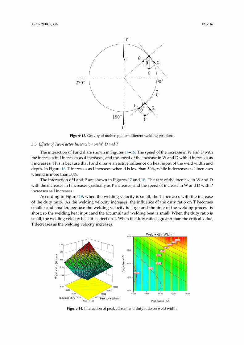
interval, the molten pool is subjected to the tangential force Gt, which leads to the molten liquid metalflowing down along the weld bead, and the flowing liquid metal can preheat the remaining weldbead and fill the weld bead, so the shape parameters of the weld width, weld depth and the weldthickness will increase with the increasing of the welding position degree. But when welding is inthe 0–90◦interval, the molten pool is subjected to the radial force Gr, and Gr = G cosθ. As the degreeof the welding position increases, the radial force becomes smaller and smaller, and the direction ofthe radial force points to the center of the pipe; In the 90–180◦ interval welding, the molten pool issubjected to the direction of the radial force back to the center of the pipe, and Gr = G sin(θ − 90);with the welding position degree increasing, Gr becomes larger and larger, hindering the increasein weld width, depth and thickness. Therefore, the slope of the curve growth is getting smaller andsmaller. Figure 12 shows the peak value of weld thickness for all values of P is received when P is 116◦.

Metals 2018, 8, 756 11 of 16Metals 2018, 8, x FOR PEER REVIEW 11 of 16
Figure 10. Influence of welding position on weld width.
Figure 11. Influence of welding position on weld depth.
Figure 12. Influence of welding position on weld thickness.
Design-Expert?Software
Factor Coding: Actual
W
X1 = D: P
Actual Factors
A: I = 120.00
B: V = 63.00
C: d = 50.00
0.00 45.00 90.00 135.00 180.00
Welding position (P),degree
We
ld w
idth
(W
),m
m
0.000
1.000
2.000
3.000
4.000
5.000
6.000
One Factor
Design-Expert?Software
Factor Coding: Actual
D
X1 = D: P
Actual Factors
A: I = 120.00
B: V = 63.00
C: d = 50.00
0.00 45.00 90.00 135.00 180.00
Welding position (P),degree
We
ld d
ep
th (
D),
mm
0.000
0.375
0.750
1.125
1.500
One Factor
Design-Expert?Software
Factor Coding: Actual
T
X1 = D: P
Actual Factors
A: I = 120.00
B: V = 63.00
C: d = 50.00
0.00 45.00 90.00 135.00 180.00
Welding position (P),degree
We
ld th
ickn
ess (
T),
mm
0.000
0.500
1.000
1.500
2.000
2.500
3.000
One Factor
Figure 10. Influence of welding position on weld width.
Metals 2018, 8, x FOR PEER REVIEW 11 of 16
Figure 10. Influence of welding position on weld width.
Figure 11. Influence of welding position on weld depth.
Figure 12. Influence of welding position on weld thickness.
Design-Expert?Software
Factor Coding: Actual
W
X1 = D: P
Actual Factors
A: I = 120.00
B: V = 63.00
C: d = 50.00
0.00 45.00 90.00 135.00 180.00
Welding position (P),degree
We
ld w
idth
(W
),m
m
0.000
1.000
2.000
3.000
4.000
5.000
6.000
One Factor
Design-Expert?Software
Factor Coding: Actual
D
X1 = D: P
Actual Factors
A: I = 120.00
B: V = 63.00
C: d = 50.00
0.00 45.00 90.00 135.00 180.00
Welding position (P),degree
We
ld d
ep
th (
D),
mm
0.000
0.375
0.750
1.125
1.500
One Factor
Design-Expert?Software
Factor Coding: Actual
T
X1 = D: P
Actual Factors
A: I = 120.00
B: V = 63.00
C: d = 50.00
0.00 45.00 90.00 135.00 180.00
Welding position (P),degree
We
ld th
ickn
ess (
T),
mm
0.000
0.500
1.000
1.500
2.000
2.500
3.000
One Factor
Figure 11. Influence of welding position on weld depth.
Metals 2018, 8, x FOR PEER REVIEW 11 of 16
Figure 10. Influence of welding position on weld width.
Figure 11. Influence of welding position on weld depth.
Figure 12. Influence of welding position on weld thickness.
Design-Expert?Software
Factor Coding: Actual
W
X1 = D: P
Actual Factors
A: I = 120.00
B: V = 63.00
C: d = 50.00
0.00 45.00 90.00 135.00 180.00
Welding position (P),degree
We
ld w
idth
(W
),m
m0.000
1.000
2.000
3.000
4.000
5.000
6.000
One Factor
Design-Expert?Software
Factor Coding: Actual
D
X1 = D: P
Actual Factors
A: I = 120.00
B: V = 63.00
C: d = 50.00
0.00 45.00 90.00 135.00 180.00
Welding position (P),degree
We
ld d
ep
th (
D),
mm
0.000
0.375
0.750
1.125
1.500
One Factor
Design-Expert?Software
Factor Coding: Actual
T
X1 = D: P
Actual Factors
A: I = 120.00
B: V = 63.00
C: d = 50.00
0.00 45.00 90.00 135.00 180.00
Welding position (P),degree
We
ld th
ickn
ess (
T),
mm
0.000
0.500
1.000
1.500
2.000
2.500
3.000
One Factor
Figure 12. Influence of welding position on weld thickness.
Metals 2018, 8, 756 12 of 16
Metals 2018, 8, x FOR PEER REVIEW 12 of 16
0°
90°
180°
270°
G
GtGr
θ
G
GrGt
G
G
G
θ
Figure 13. Gravity of molten pool at different welding positions.
5.5. Effects of Two-Factor Interaction on W, D and T
The interaction of I and d are shown in Figures 14, 15 and 16. The speed of the increase in W and
D with the increases in I increases as d increases, and the speed of the increase in W and D with d
increases as I increases. This is because that I and d have an active influence on heat input of the weld
width and depth. In Figure 16, T increases as I increases when d is less than 50%, while it decreases
as I increases when d is more than 50%.
The interaction of I and P are shown in Figures 17 and 18. The rate of the increase in W and D
with the increases in I increases gradually as P increases, and the speed of increase in W and D with
P increases as I increases.
According to Figure 19, when the welding velocity is small, the T increases with the increase of
the duty ratio. As the welding velocity increases, the influence of the duty ratio on T becomes smaller
and smaller, because the welding velocity is large and the time of the welding process is short, so the
welding heat input and the accumulated welding heat is small. When the duty ratio is small, the
welding velocity has little effect on T. When the duty ratio is greater than the critical value, T
decreases as the welding velocity increases.
Figure 14. Interaction of peak current and duty ratio on weld width.
Design-Expert?SoftwareFactor Coding: ActualW (mm)
5.86
0.99
X1 = A: IX2 = C: d
Actual FactorsB: V = 63.00D: P = 90.00
40.00
45.00
50.00
55.00
60.00
114.00
117.00
120.00
123.00
126.00
0.00
2.00
4.00
6.00
8.00
Weld
wid
th (
W),
mm
Peak current (I),mmDuty ratio (d),%
Design-Expert?Software
Factor Coding: Actual
W
5.859
0.987
X1 = A: I
X2 = C: d
Actual Factors
B: V = 63.00
D: P = 90.00
114.00 117.00 120.00 123.00 126.00
40.00
45.00
50.00
55.00
60.00Weld width (W),mm
Peak current (I),A
Du
ty r
atio
o (
d),
%
2.000
2.500
3.000
3.500
4.000
4.500
5.0005.500
6.000
Figure 13. Gravity of molten pool at different welding positions.
5.5. Effects of Two-Factor Interaction on W, D and T
The interaction of I and d are shown in Figures 14–16. The speed of the increase in W and D withthe increases in I increases as d increases, and the speed of the increase in W and D with d increases asI increases. This is because that I and d have an active influence on heat input of the weld width anddepth. In Figure 16, T increases as I increases when d is less than 50%, while it decreases as I increaseswhen d is more than 50%.
The interaction of I and P are shown in Figures 17 and 18. The rate of the increase in W and Dwith the increases in I increases gradually as P increases, and the speed of increase in W and D with Pincreases as I increases.
According to Figure 19, when the welding velocity is small, the T increases with the increaseof the duty ratio. As the welding velocity increases, the influence of the duty ratio on T becomessmaller and smaller, because the welding velocity is large and the time of the welding process isshort, so the welding heat input and the accumulated welding heat is small. When the duty ratio issmall, the welding velocity has little effect on T. When the duty ratio is greater than the critical value,T decreases as the welding velocity increases.
Metals 2018, 8, x FOR PEER REVIEW 12 of 16
0°
90°
180°
270°
G
GtGr
θ
G
GrGt
G
G
G
θ
Figure 13. Gravity of molten pool at different welding positions.
5.5. Effects of Two-Factor Interaction on W, D and T
The interaction of I and d are shown in Figures 14, 15 and 16. The speed of the increase in W and D with the increases in I increases as d increases, and the speed of the increase in W and D with d increases as I increases. This is because that I and d have an active influence on heat input of the weld width and depth. In Figure 16, T increases as I increases when d is less than 50%, while it decreases as I increases when d is more than 50%.
The interaction of I and P are shown in Figures 17 and 18. The rate of the increase in W and D with the increases in I increases gradually as P increases, and the speed of increase in W and D with P increases as I increases.
According to Figure 19, when the welding velocity is small, the T increases with the increase of the duty ratio. As the welding velocity increases, the influence of the duty ratio on T becomes smaller and smaller, because the welding velocity is large and the time of the welding process is short, so the welding heat input and the accumulated welding heat is small. When the duty ratio is small, the welding velocity has little effect on T. When the duty ratio is greater than the critical value, T decreases as the welding velocity increases.
Figure 14. Interaction of peak current and duty ratio on weld width.
40.00
45.00
50.00
55.00
60.00
114.00
117.00
120.00
123.00
126.00
0.00
2.00
4.00
6.00
8.00
Wel
d w
idth
(W),m
m
Peak current (I),mmDuty ratio (d),%114.00 117.00 120.00 123.00 126.00
40.00
45.00
50.00
55.00
60.00Weld width (W),mm
Peak current (I),A
Dut
y ra
tioo
(d),%
2.000
2.500
3.000
3.500
4.0004.500
5.0005.500
6.000
Figure 14. Interaction of peak current and duty ratio on weld width.

Metals 2018, 8, 756 13 of 16Metals 2018, 8, x FOR PEER REVIEW 13 of 16
Figure 15. Interaction of peak current and duty ratio on weld depth.
Figure 16. Interaction of peak current and duty ratio on weld thickness.
Figure 17. Interaction of peak current and welding position on weld width.
40.00
45.00
50.00
55.00
60.00
114.00
117.00
120.00
123.00
126.00
0
0.5
1
1.5
2 W
eld
dept
h (D
),mm
Peak current (I),mmDuty ratio (d),%
114.00 116.00 118.00 120.00 122.00 124.00 126.00
40.00
44.00
48.00
52.00
56.00
60.00Weld depth (D),mm
Peak current (I),A
Dut
y ra
tio (d
),%
0.400
0.600
0.800
1.000
1.200
1.400
45.00 47.50
50.00 52.50
55.00
114.00
117.00
120.00
123.00
126.00
1.5
2
2.5
3
3.5
Wel
d th
ickn
ess
(T) ,
mm
Peak current (I),ADuty ratio (d), %
114.00 117.00 120.00 123.00 126.00
40.00
44.00
48.00
52.00
56.00
60.00Weld thickness (T),mm
Peak current (I),A
Dut
y ra
tio (d
),%
2.000
2.500
2.599
2.363
2.168
1.812
2.738
0.00
45.00
90.00
135.00
180.00
114.00
117.00
120.00
123.00
126.00
0.00
2.00
4.00
6.00
8.00
Wel
d w
idth
(W),m
m
Peak current (I),mmWelding position (P),degree
114.00 117.00 120.00 123.00 126.00
0.00
45.00
90.00
135.00
180.00Weld width (W),mm
Peak current (I),A
Wel
ding
pos
ition
(P),d
egre
e
0.500
1.000
1.500
2.000
2.500
3.000
3.500
4.000
4.500
5.000
5.500
6.000
Figure 15. Interaction of peak current and duty ratio on weld depth.
Metals 2018, 8, x FOR PEER REVIEW 13 of 16
Figure 15. Interaction of peak current and duty ratio on weld depth.
Figure 16. Interaction of peak current and duty ratio on weld thickness.
Figure 17. Interaction of peak current and welding position on weld width.
40.00
45.00
50.00
55.00
60.00
114.00
117.00
120.00
123.00
126.00
0
0.5
1
1.5
2 W
eld
dept
h (D
),mm
Peak current (I),mmDuty ratio (d),%
114.00 116.00 118.00 120.00 122.00 124.00 126.00
40.00
44.00
48.00
52.00
56.00
60.00Weld depth (D),mm
Peak current (I),A
Dut
y ra
tio (d
),%
0.400
0.600
0.800
1.000
1.200
1.400
45.00 47.50
50.00 52.50
55.00
114.00
117.00
120.00
123.00
126.00
1.5
2
2.5
3
3.5
Wel
d th
ickn
ess
(T) ,
mm
Peak current (I),ADuty ratio (d), %
114.00 117.00 120.00 123.00 126.00
40.00
44.00
48.00
52.00
56.00
60.00Weld thickness (T),mm
Peak current (I),A
Dut
y ra
tio (d
),%
2.000
2.500
2.599
2.363
2.168
1.812
2.738
0.00
45.00
90.00
135.00
180.00
114.00
117.00
120.00
123.00
126.00
0.00
2.00
4.00
6.00
8.00
Wel
d w
idth
(W),m
m
Peak current (I),mmWelding position (P),degree
114.00 117.00 120.00 123.00 126.00
0.00
45.00
90.00
135.00
180.00Weld width (W),mm
Peak current (I),A
Wel
ding
pos
ition
(P),d
egre
e
0.500
1.000
1.500
2.000
2.500
3.000
3.500
4.000
4.500
5.000
5.500
6.000
Figure 16. Interaction of peak current and duty ratio on weld thickness.
Metals 2018, 8, x FOR PEER REVIEW 13 of 16
Figure 15. Interaction of peak current and duty ratio on weld depth.
Figure 16. Interaction of peak current and duty ratio on weld thickness.
Figure 17. Interaction of peak current and welding position on weld width.
40.00
45.00
50.00
55.00
60.00
114.00
117.00
120.00
123.00
126.00
0
0.5
1
1.5
2 W
eld
dept
h (D
),mm
Peak current (I),mmDuty ratio (d),%
114.00 116.00 118.00 120.00 122.00 124.00 126.00
40.00
44.00
48.00
52.00
56.00
60.00Weld depth (D),mm
Peak current (I),A
Dut
y ra
tio (d
),%
0.400
0.600
0.800
1.000
1.200
1.400
45.00 47.50
50.00 52.50
55.00
114.00
117.00
120.00
123.00
126.00
1.5
2
2.5
3
3.5
Wel
d th
ickn
ess
(T) ,
mm
Peak current (I),ADuty ratio (d), %
114.00 117.00 120.00 123.00 126.00
40.00
44.00
48.00
52.00
56.00
60.00Weld thickness (T),mm
Peak current (I),A
Dut
y ra
tio (d
),%
2.000
2.500
2.599
2.363
2.168
1.812
2.738
0.00
45.00
90.00
135.00
180.00
114.00
117.00
120.00
123.00
126.00
0.00
2.00
4.00
6.00
8.00
Wel
d w
idth
(W),m
m
Peak current (I),mmWelding position (P),degree
114.00 117.00 120.00 123.00 126.00
0.00
45.00
90.00
135.00
180.00Weld width (W),mm
Peak current (I),A
Wel
ding
pos
ition
(P),d
egre
e
0.500
1.000
1.500
2.000
2.500
3.000
3.500
4.000
4.500
5.000
5.500
6.000
Figure 17. Interaction of peak current and welding position on weld width.

Metals 2018, 8, 756 14 of 16Metals 2018, 8, x FOR PEER REVIEW 14 of 16
Figure 18. Interaction of peak current and welding position on weld depth.
Figure 19. Interaction of weld velocity and duty ratio on weld thickness.
5.6. Optimization of the Welding Parameters by Numerical Method
In order to obtain the ideal weld bead shape and avoid welding defects such as incomplete penetration and weld collapse, numerical analysis was used to optimize the welding parameters. The goal, lower, upper limits and importance for every input and response parameters of the standard are shown in Table 8. Table 9 lists optimal welding parameters at 0, 45°, 90°, 135° and 180° welding position. The Figure 20 has shown the cross sections of weld bead with the optimal parameters at disparate welding position in 0–180°, it shows that the gap between tubes is different for each case; there are two factors lead to this phenomenon. One factor is welding deformation: the welding process generates a lot of heat, which lead to pipes deformation. The other factor is welding sequence: welding experiments weld the bead at the 0° position firstly, so the weld bead was solidified first at the 0° welding position, which results in other gaps between tubes being confirmed.
0.00
45.00
90.00
135.00
180.00
114.00
117.00
120.00
123.00
126.00
0
0.5
1
1.5
2 W
eld
dept
h (D
),mm
Peak current (I),mmWelding position (P),degree
114.00 116.00 118.00 120.00 122.00 124.00 126.00
0.00
45.00
90.00
135.00
180.00Weld depth (D),mm
Peak current (I),A
Wel
ding
pos
ition
(P),d
egre
e
0.200
0.400
0.600
0.800
1.000
1.200
45.00
47.50
50.00
52.50
55.00
57.00
60.00
63.00
66.00
69.00
1.5
2
2.5
3
3.5
Wel
d th
ickn
ess
(T) ,
mm
Weld velocity (V), mm/minDuty ratio (d), %
57.00 60.00 63.00 66.00 69.00
40.00
44.00
48.00
52.00
56.00
60.00Weld thickness (T),mm
Weld velocity (V),mm/min
Dut
y ra
tio (d
),%
2.000
2.000
2.168
2.363
2.5002.599
2.738
3.000
Figure 18. Interaction of peak current and welding position on weld depth.
Metals 2018, 8, x FOR PEER REVIEW 14 of 16
Figure 18. Interaction of peak current and welding position on weld depth.
Figure 19. Interaction of weld velocity and duty ratio on weld thickness.
5.6. Optimization of the Welding Parameters by Numerical Method
In order to obtain the ideal weld bead shape and avoid welding defects such as incomplete penetration and weld collapse, numerical analysis was used to optimize the welding parameters. The goal, lower, upper limits and importance for every input and response parameters of the standard are shown in Table 8. Table 9 lists optimal welding parameters at 0, 45°, 90°, 135° and 180° welding position. The Figure 20 has shown the cross sections of weld bead with the optimal parameters at disparate welding position in 0–180°, it shows that the gap between tubes is different for each case; there are two factors lead to this phenomenon. One factor is welding deformation: the welding process generates a lot of heat, which lead to pipes deformation. The other factor is welding sequence: welding experiments weld the bead at the 0° position firstly, so the weld bead was solidified first at the 0° welding position, which results in other gaps between tubes being confirmed.
0.00
45.00
90.00
135.00
180.00
114.00
117.00
120.00
123.00
126.00
0
0.5
1
1.5
2 W
eld
dept
h (D
),mm
Peak current (I),mmWelding position (P),degree
114.00 116.00 118.00 120.00 122.00 124.00 126.00
0.00
45.00
90.00
135.00
180.00Weld depth (D),mm
Peak current (I),A
Wel
ding
pos
ition
(P),d
egre
e
0.200
0.400
0.600
0.800
1.000
1.200
45.00
47.50
50.00
52.50
55.00
57.00
60.00
63.00
66.00
69.00
1.5
2
2.5
3
3.5
Wel
d th
ickn
ess
(T) ,
mm
Weld velocity (V), mm/minDuty ratio (d), %
57.00 60.00 63.00 66.00 69.00
40.00
44.00
48.00
52.00
56.00
60.00Weld thickness (T),mm
Weld velocity (V),mm/min
Dut
y ra
tio (d
),%
2.000
2.000
2.168
2.363
2.5002.599
2.738
3.000
Figure 19. Interaction of weld velocity and duty ratio on weld thickness.
5.6. Optimization of the Welding Parameters by Numerical Method
In order to obtain the ideal weld bead shape and avoid welding defects such as incompletepenetration and weld collapse, numerical analysis was used to optimize the welding parameters.The goal, lower, upper limits and importance for every input and response parameters of the standardare shown in Table 8. Table 9 lists optimal welding parameters at 0, 45◦, 90◦, 135◦ and 180◦ weldingposition. The Figure 20 has shown the cross sections of weld bead with the optimal parameters atdisparate welding position in 0–180◦, it shows that the gap between tubes is different for each case;there are two factors lead to this phenomenon. One factor is welding deformation: the welding processgenerates a lot of heat, which lead to pipes deformation. The other factor is welding sequence: weldingexperiments weld the bead at the 0◦ position firstly, so the weld bead was solidified first at the 0◦
welding position, which results in other gaps between tubes being confirmed.
Table 8. Restraint of numerical optimization.
Name Goal Lower Upper Importance
I Is in range 114 126 3V Is in range 57 69 3d Is in range 40 60 3P Is equal to 0 180 3W maximize 0.987 5.859 5D Is in range 0.8 1.5 5T Is in range 1.533 3.204 5

Metals 2018, 8, 756 15 of 16
Table 9. Optimal parameters.
I (A) V (mm/min) d (%) P (Degree)
126 57 60 0125 58 59 45124 60 58 90122 60 54 135119 61 54 180
Metals 2018, 8, x FOR PEER REVIEW 14 of 16
Figure 18. Interaction of peak current and welding position on weld depth.
Figure 19. Interaction of weld velocity and duty ratio on weld thickness.
5.6. Optimization of the Welding Parameters by Numerical Method
In order to obtain the ideal weld bead shape and avoid welding defects such as incomplete
penetration and weld collapse, numerical analysis was used to optimize the welding parameters. The
goal, lower, upper limits and importance for every input and response parameters of the standard
are shown in Table 8. Table 9 lists optimal welding parameters at 0, 45°, 90°, 135° and 180° welding
position. The Figure 20 has shown the cross sections of weld bead with the optimal parameters at
disparate welding position in 0–180°, it shows that the gap between tubes is different for each case;
there are two factors lead to this phenomenon. One factor is welding deformation: the welding
process generates a lot of heat, which lead to pipes deformation. The other factor is welding sequence:
welding experiments weld the bead at the 0° position firstly, so the weld bead was solidified first at
the 0° welding position, which results in other gaps between tubes being confirmed.
Design-Expert?SoftwareFactor Coding: ActualD (mm)
1.298
0.199
X1 = A: IX2 = D: P
Actual FactorsB: V = 63.00C: d = 50.00
0.00
45.00
90.00
135.00
180.00
114.00
117.00
120.00
123.00
126.00
0
0.5
1
1.5
2
Weld
depth
(D
),m
m
Peak current (I),mmWelding position (P),degree
Design-Expert?Software
Factor Coding: Actual
D
1.298
0.199
X1 = A: I
X2 = D: P
Actual Factors
B: V = 63.00
C: d = 50.00
114.00 116.00 118.00 120.00 122.00 124.00 126.00
0.00
45.00
90.00
135.00
180.00Weld depth (D),mm
Peak current (I),A
We
ldin
g p
ositio
n (
P),
de
gre
e
0.200
0.400
0.600
0.800
1.000
1.200
Design-Expert?SoftwareFactor Coding: ActualT (mm)
3.024
1.533
X1 = B: VX2 = C: d
Actual FactorsA: I = 120.00D: P = 90.00
45.00
47.50
50.00
52.50
55.00
57.00
60.00
63.00
66.00
69.00
1.5
2
2.5
3
3.5
Weld
thic
kness (
T)
,mm
Weld velocity (V), mm/minDuty ratio (d), %
Design-Expert?Software
Factor Coding: Actual
T
3.024
1.533
X1 = B: V
X2 = C: d
Actual Factors
A: I = 120.00
D: P = 90.00
57.00 60.00 63.00 66.00 69.00
40.00
44.00
48.00
52.00
56.00
60.00Weld thickness (T),mm
Weld velocity (V),mm/min
Du
ty r
atio
(d
),%
2.000
2.000
2.168
2.363
2.500
2.599
2.738
3.000
Metals 2018, 8, x FOR PEER REVIEW 15 of 16
Figure 20. Cross sections of weld bead at different welding position from 0–180°. (a) 0° welding
position, (b) 45° welding position, (c) 90° welding position, (d) 135° welding position.
Table 8. Restraint of numerical optimization.
Name Goal Lower Upper Importance
I Is in range 114 126 3
V Is in range 57 69 3
d Is in range 40 60 3
P Is equal to 0 180 3
W maximize 0.987 5.859 5
D Is in range 0.8 1.5 5
T Is in range 1.533 3.204 5
Table 9. Optimal parameters.
I (A) V (mm/min) d (%) P (Degree)
126 57 60 0
125 58 59 45
124 60 58 90
122 60 54 135
119 61 54 180
6. Conclusions
In this research, the all-position automatic welding of pipes has been researched and statistically
analysed. The main conclusions drawn from this research are as follows:
(1) Response surface methodology (RSM) based on center composed design (CCD) can be used
to establish a mathematical model, and it can predict weld bead shape in the all-position automatic
welding of pipes.
(2) Weld peak current had a prominent active influence on the important weld bead geometry
parameters, while welding velocity had a negative influence on the important weld bead geometry
parameters. The duty ratio exhibits a quadratic parabolic relationship with W and D, and the slope
of the curve increases as the duty ratio increases, while T and the duty ratio increase linearly. The
welding position has a quadratic parabolic relationship with the important weld bead geometry
parameters, and the slope of the curve decreases as the degree of the welding position increases.
(3). The ideal weld bead geometry can be obtained by choosing the optimal weld parameters
with the established statistical models, and this model can be used for the all-position automatic
welding of pipes
Author contributions: B.L. performed the experiments, analyzed the data, and wrote the original manuscript.
Y.S. conceived and designed the experiments, and contributed significantly to analysis and manuscript
improvement. Y.C. and S.C. helped perform the analysis with constructive discussions. Z.J. and Y.Y. helped
perform the experiments and analyse the data.
Funding: This research was funded by Science and Technology Planning Project of Guangzhou City (Grant No.
201604046026), Science and Technology Planning Project of Guangdong Province (Grant No. 2015B010919005),
and National Natural Science Foundation of China (Grant No. 51374111).
Acknowledgments: The authors gratefully acknowledge Guangzhou Shipyard International Company Limited
for providing experimental materials.
Figure 20. Cross sections of weld bead at different welding position from 0–180◦. (a) 0◦ weldingposition, (b) 45◦ welding position, (c) 90◦ welding position, (d) 135◦ welding position.
6. Conclusions
In this research, the all-position automatic welding of pipes has been researched and statisticallyanalysed. The main conclusions drawn from this research are as follows:
(1) Response surface methodology (RSM) based on center composed design (CCD) can be used toestablish a mathematical model, and it can predict weld bead shape in the all-position automaticwelding of pipes.
(2) Weld peak current had a prominent active influence on the important weld bead geometryparameters, while welding velocity had a negative influence on the important weld bead geometryparameters. The duty ratio exhibits a quadratic parabolic relationship with W and D, and theslope of the curve increases as the duty ratio increases, while T and the duty ratio increaselinearly. The welding position has a quadratic parabolic relationship with the important weldbead geometry parameters, and the slope of the curve decreases as the degree of the weldingposition increases.
(3) The ideal weld bead geometry can be obtained by choosing the optimal weld parameters with theestablished statistical models, and this model can be used for the all-position automatic weldingof pipes.
Author Contributions: B.L. performed the experiments, analyzed the data, and wrote the original manuscript.Y.S. conceived and designed the experiments, and contributed significantly to analysis and manuscriptimprovement. Y.C. and S.C. helped perform the analysis with constructive discussions. Z.J. and Y.Y. helpedperform the experiments and analyse the data.
Funding: This research was funded by Science and Technology Planning Project of Guangzhou City (GrantNo. 201604046026), Science and Technology Planning Project of Guangdong Province (Grant No. 2015B010919005),and National Natural Science Foundation of China (Grant No. 51374111).
Acknowledgments: The authors gratefully acknowledge Guangzhou Shipyard International Company Limitedfor providing experimental materials.
Conflicts of Interest: The authors declare no conflict of interest.

Metals 2018, 8, 756 16 of 16
References
1. Xu, W.H.; Lin, S.B.; Fan, C.L.; Zhuo, X.Q.; Yang, C.L. Statistical modelling of weld bead geometry in oscillatingarc narrow gap all-position GMA welding. Int. J. Adv. Manuf. Technol. 2014, 72, 1705–1716. [CrossRef]
2. Manonmani, K.; Murugan, N.; Buvanasekaran, G. Effects of process parameters on the bead geometry oflaser beam butt welded stainless steel sheets. Int. J. Adv. Manuf. Technol. 2007, 32, 1125–1133. [CrossRef]
3. Kim, D.I.S.; Basu, A.; Siores, E. Mathematical models for control of weld bead penetration in the GMAWprocess. Int. J. Adv. Manuf. Technol. 1996, 12, 393–401. [CrossRef]
4. Xu, W.H.; Lin, S.B.; Fan, C.L.; Yang, C.L. Prediction and optimization of weld bead geometry in oscillatingarc narrow gap all-position GMA welding. Int. J. Adv. Manuf. Technol. 2015, 79, 183–196. [CrossRef]
5. Rao, P.S.; Gupta, O.P.; Murty, S.S.N.; Rao, A.B.K. Effect of process parameters and mathematical model forthe prediction of bead geometry in pulsed GMA welding. Int. J. Adv. Manuf. Technol. 2009, 45, 496–505.[CrossRef]
6. Koleva, E. Electron beam weld parameters and thermal efficiency improvement. Vacuum 2005, 77, 413–421.[CrossRef]
7. Karthikeyan, R.; Balasubramanian, V. Predictions of the optimized friction stir spot welding processparameters for joining AA2024 aluminum alloy using RSM. Int. J. Adv. Manuf. Technol. 2010, 51, 173–183.[CrossRef]
8. Ii, E.J.L.; Torres, G.C.F.; Felizardo, I.; Filho, F.A.R.; Bracarense, A.Q. Development of a robot for orbitalwelding. Ind. Robot 2005, 32, 321–325.
9. Acherjee, B.; Kuar, A.S.; Mitra, S.; Misra, D. Modeling and analysis of simultaneous laser transmissionwelding of polycarbonates using an FEM and RSM combined approach. Opt. Laser Technol. 2012, 44,995–1006. [CrossRef]
10. Gunaraj, V.; Murugan, N. Application of response surface methodology for predicting weld bead quality insubmerged arc welding of pipes. J. Mater. Process. Technol. 1999, 88, 266–275. [CrossRef]
11. Acherjee, B.; Misra, D.; Bose, D.; Venkadeshwaran, K. Prediction of weld strength and seam width for lasertransmission welding of thermoplastic using response surface methodology. Opt. Laser Technol. 2009, 41,956–967. [CrossRef]
12. Ruggiero, A.; Tricarico, L.; Olabi, A.G.; Benyounis, K.Y. Weld-bead profile and costs optimisation of the CO2
dissimilar laser welding process of low carbon steel and austenitic steel AISI316. Opt. Laser Technol. 2011, 43,82–90. [CrossRef]
13. Gunaraj, V.; Murugan, N. Prediction and comparison of the area of the heat-affected zone for thebead-on-plate and bead-on-joint in submerged arc welding of pipes. J. Mater. Process. Technol. 1999,95, 246–261. [CrossRef]
14. Murugan, N.; Gunaraj, V. Prediction and control of weld bead geometry and shape relationships insubmerged arc welding of pipes. J. Mater. Process. Technol. 2005, 168, 478–487. [CrossRef]
15. Rajakumar, S.; Balasubramanian, V. Diffusion bonding of titanium and AA7075 aluminum alloy dissimilarjoints—Process modeling and optimization using desirability approach. Int. J. Adv. Manuf. Technol. 2016, 86,1–18. [CrossRef]
16. Colombini, E.; Sola, R.; Parigi, G.; Veronesi, P.; Poli, G. Laser quenching of ionic nitrided steel: Effectof process parameters on microstructure and optimization. Metall. Mater. Trans. A 2014, 45, 5562–5573.[CrossRef]
17. Poli, G.; Sola, R.; Veronesi, P. Microwave-assisted combustion synthesis of NiAl intermetallics in a singlemode applicator: Modeling and optimisation. Mater. Sci. Eng. A 2006, 441, 149–156. [CrossRef]
© 2018 by the authors. Licensee MDPI, Basel, Switzerland. This article is an open accessarticle distributed under the terms and conditions of the Creative Commons Attribution(CC BY) license (http://creativecommons.org/licenses/by/4.0/).