mathematical foundations of data sciences0, it still makes sense to consider in nite dimensional...
TRANSCRIPT

Mathematical Foundations of Data Sciences
Gabriel PeyreCNRS & DMA
Ecole Normale [email protected]
https://mathematical-tours.github.io
www.numerical-tours.com
October 6, 2019

2
Chapter 1
Inverse Problems
The main references for this chapter are [1, ?, ?].
1.1 Inverse Problems Regularization
Increasing the resolution of signals and images requires to solve an ill posed inverse problem. Thiscorresponds to inverting a linear measurement operator that reduces the resolution of the image. Thischapter makes use of convex regularization introduced in Chapter ?? to stabilize this inverse problem.
We consider a (usually) continuous linear map Φ : S → H where S can be an Hilbert or a more generalBanach space. This operator is intended to capture the hardware acquisition process, which maps a highresolution unknown signal f0 ∈ S to a noisy low-resolution obervation
y = Φf0 + w ∈ H
where w ∈ H models the acquisition noise. In this section, we do not use a random noise model, and simplyassume that ||w||H is bounded.
In most applications, H = RP is finite dimensional, because the hardware involved in the acquisitioncan only record a finite (and often small) number P of observations. Furthermore, in order to implementnumerically a recovery process on a computer, it also makes sense to restrict the attention to S = RN , whereN is number of point on the discretization grid, and is usually very large, N P . However, in order toperform a mathematical analysis of the recovery process, and to be able to introduce meaningful models onthe unknown f0, it still makes sense to consider infinite dimensional functional space (especially for the dataspace S).
The difficulty of this problem is that the direct inversion of Φ is in general impossible or not advisablebecause Φ−1 have a large norm or is even discontinuous. This is further increased by the addition of somemeasurement noise w, so that the relation Φ−1y = f0 +Φ−1w would leads to an explosion of the noise Φ−1w.
We now gives a few representative examples of forward operators Φ.
Denoising. The case of the identity operator Φ = IdS , S = H corresponds to the classical denoisingproblem, already treated in Chapters ?? and ??.
De-blurring and super-resolution. For a general operator Φ, the recovery of f0 is more challenging,and this requires to perform both an inversion and a denoising. For many problem, this two goals are incontradiction, since usually inverting the operator increases the noise level. This is for instance the case forthe deblurring problem, where Φ is a translation invariant operator, that corresponds to a low pass filteringwith some kernel h
Φf = f ? h. (1.1)
3

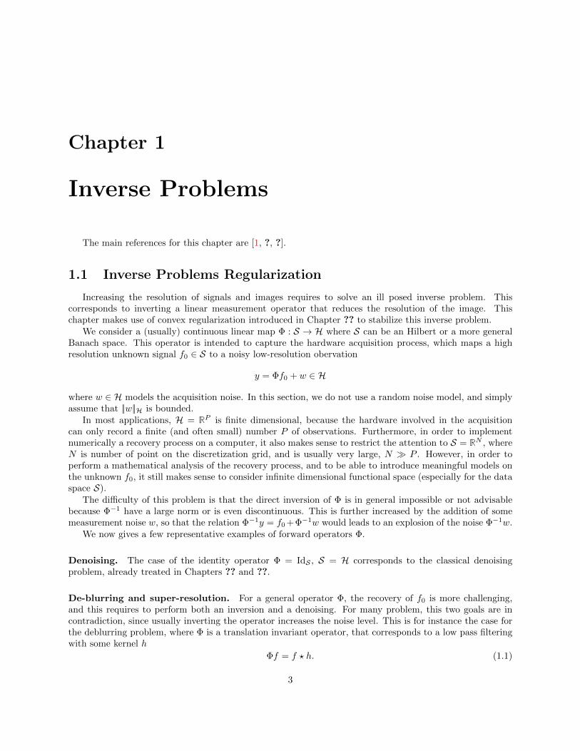
One can for instance consider this convolution over S = H = L2(Td), see Proposition ??. In practice, thisconvolution is followed by a sampling on a grid Φf = (f ? h)(xk) ; 0 6 k < P, see Figure 1.1, middle, foran example of a low resolution image Φf0. Inverting such operator has important industrial application toupsample the content of digital photos and to compute high definition videos from low definition videos.
Interpolation and inpainting. Inpainting corresponds to interpolating missing pixels in an image. Thisis modelled by a diagonal operator over the spacial domain
(Φf)(x) =
0 if x ∈ Ω,f(x) if x /∈ Ω.
(1.2)
where Ω ⊂ [0, 1]d (continuous model) or 0, . . . , N − 1 which is then a set of missing pixels. Figure 1.1,right, shows an example of damaged image Φf0.
Original f0 Low resolution Φf0 Masked Φf0
Figure 1.1: Example of inverse problem operators.
Medical imaging. Most medical imaging acquisition device only gives indirect access to the signal ofinterest, and is usually well approximated by such a linear operator Φ. In scanners, the acquisition operator isthe Radon transform, which, thanks to the Fourier slice theorem, is equivalent to partial Fourier mesurmentsalong radial lines. Medical resonance imaging (MRI) is also equivalent to partial Fourier measures
Φf =f(x) ; x ∈ Ω
. (1.3)
Here, Ω is a set of radial line for a scanner, and smooth curves (e.g. spirals) for MRI.Other indirect application are obtained by electric or magnetic fields measurements of the brain activity
(corresponding to MEG/EEG). Denoting Ω ⊂ R3 the region around which measurements are performed (e.g.the head), in a crude approximation of these measurements, one can assume Φf = (ψ ? f)(x) ; x ∈ ∂Ωwhere ψ(x) is a kernel accounting for the decay of the electric or magnetic field, e.g. ψ(x) = 1/||x||2.
Regression for supervised learning. While the focus of this chapter is on imaging science, a closely re-lated problem is supervised learning using linear model. The typical notations associated to this problem areusually different, which causes confusion. This problem is detailed in Chapter ??, which draws connectionbetween regression and inverse problems. In statistical learning, one observes pairs (xi, yi)
ni=1 of n observa-
tion, where the features are xi ∈ Rp. One seeks for a linear prediction model of the form yi = 〈β, xi〉 wherethe unknown parameter is β ∈ Rp. Storing all the xi as rows of a matrix X ∈ Rn×p, supervised learningaims at approximately solving Xβ ≈ y. The problem is similar to the inverse problem Φf = y where one
4

performs the change of variable Φ 7→ X and f 7→ β, with dimensions (P,N)→ (n, p). In statistical learning,one does not assume some well specified model y = Φf0 +w, and the major difference is that the matrix Xis random, which add extra “noise” which needs to be controlled as n→ +∞. The recovery is performed bythe normalized ridge regression problem
minβ
1
2n||Xβ − y||2 + λ||β||2
so that the natural change of variable should be 1nX∗X ∼ Φ∗Φ (empirical covariance) and 1
nX∗y ∼ Φ∗y.
The law of large number shows that 1nX∗X and 1
nX∗y are contaminated by a noise of amplitude 1/
√n,
which plays the role of ||w||.
1.2 Theoretical Study of Quadratic Regularization
We now give a glimpse on the typical approach to obtain theoretical guarantee on recovery quality in thecase of Hilbert space. The goal is not to be exhaustive, but rather to insist on the modelling hypotethese,namely smoothness implies a so called “source condition”, and the inherent limitations of quadratic methods(namely slow rates and the impossibility to recover information in ker(Φ), i.e. to achieve super-resolution).
1.2.1 Singular Value Decomposition
Finite dimension. Let us start by the simple finite dimensional case Φ ∈ RP×N so that S = RN andH = RP are Hilbert spaces. In this case, the Singular Value Decomposition (SVD) is the key to analyze theoperator very precisely, and to describe linear inversion process.
Proposition 1 (SVD). There exists (U, V ) ∈ RP×R × RN×R, where R = rank(Φ) = dim(Im(Φ)), withU>U = V >V = IdR, i.e. having orthogonal columns (um)Rm=1 ⊂ RN , (vm)Rm=1 ⊂ RP , and (σm)Rm=1 withσm > 0, such that
Φ = U diagm(σm)V > =
R∑m=1
σmumv>m. (1.4)
Proof. We first analyze the problem, and notice that if Φ = UΣV > with Σ = diagm(σm), then ΦΦ> =UΣ2U> and then V > = Σ−1U>Φ. We can use this insight. Since ΦΦ> is a positive symmetric matrix,we write its eigendecomposition as ΦΦ> = UΣ2U> where Σ = diagRm=1(σm) with σm > 0. We then define
Vdef.= Φ>UΣ−1. One then verifies that
V >V = (Σ−1U>Φ)(Φ>UΣ−1) = Σ−1U>(UΣ2U>)UΣ−1 = IdR and UΣV > = UΣΣ−1U>Φ = Φ.
This theorem is still valid with complex matrice, replacing > by ∗. Expression (1.4) describes Φ as a sumof rank-1 matrices umv
>m. One usually order the singular values (σm)m in decaying order σ1 > . . . > σR. If
these values are different, then the SVD is unique up to ±1 sign change on the singular vectors.The left singular vectors U is an orthonormal basis of Im(Φ), while the right singular values is an
orthonormal basis of Im(Φ>) = ker(Φ)⊥. The decomposition (1.4) is often call the “reduced” SVD becauseone has only kept the R non-zero singular values. The “full” SVD is obtained by completing U and V todefine orthonormal bases of the full spaces RP and RN . Then Σ becomes a rectangular matrix of size P ×N .
A typical example is for Φf = f ? h over RP = RN , in which case the Fourier transform diagonalizes theconvolution, i.e.
Φ = (um)∗m diag(hm)(um)m (1.5)
where (um)ndef.= 1√
Ne
2iπN nm so that the singular values are σm = |hm| (removing the zero values) and the
singular vectors are (um)n and (vmθm)n where θmdef.= |hm|/hm is a unit complex number.
Computing the SVD of a full matrix Φ ∈ RN×N has complexity N3.
5

Compact operators. One can extend the decomposition to compact operators Φ : S → H betweenseparable Hilbert space. A compact operator is such that ΦB1 is pre-compact where B1 = s ∈ S ; ||s|| 6 1is the unit-ball. This means that for any sequence (Φsk)k where sk ∈ B1 one can extract a convergingsub-sequence. Note that in infinite dimension, the identity operator Φ : S → S is never compact.
Compact operators Φ can be shown to be equivalently defined as those for which an expansion of theform (1.4) holds
Φ =
+∞∑m=1
σmumv>m (1.6)
where (σm)m is a decaying sequence converging to 0, σm → 0. Here in (1.6) convergence holds in the operatornorm, which is the algebra norm on linear operator inherited from those of S and H
||Φ||L(S,H)def.= min||Φu||H
||u||S 6 1.
For Φ having an SVD decomposition (1.6), ||Φ||L(S,H) = σ1.When σm = 0 for m > R, Φ has a finite rank R = dim(Im(Φ)). As we explain in the sections bellow,
when using linear recovery methods (such as quadratic regularization), the inverse problem is equivalent toa finite dimensional problem, since one can restrict its attention to functions in ker(Φ)⊥ which as dimensionR. Of course, this is not true anymore when one can retrieve function inside ker(Φ), which is often referredto as a “super-resolution” effect of non-linear methods. Another definition of compact operator is that theyare the limit of finite rank operator. They are thus in some sense the extension of finite dimensional matrices,and are the correct setting to model ill-posed inverse problems. This definition can be extended to linearoperator between Banach spaces, but this conclusion does not holds.
Typical example of compact operator are matrix-like operator with a continuous kernel k(x, y) for (x, y) ∈Ω where Ω is a compact sub-set of Rd (or the torus Td), i.e.
(Φf)(x) =
∫Ω
k(x, y)f(y)dy
where dy is the Lebesgue measure. An example of such a setting which generalizes (1.5) is when Φf = f ? hon Td = (R/2πZ)d, which is corresponds to a translation invariant kernel k(x, y) = h(x − y), in which case
um(x) = (2π)−d/2eiωx, σm = |fm|. Another example on Ω = [0, 1] is the integration, (Φf)(x) =∫ x
0f(y)dy,
which corresponds to k being the indicator of the “triangle”, k(x, y) = 1x6y.
Pseudo inverse. In the case where w = 0, it makes to try to directly solve Φf = y. The two obstructionfor this is that one not necessarily has y ∈ Im(Φ) and even so, there are an infinite number of solutions ifker(Φ) 6= 0. The usual workaround is to solve this equation in the least square sense
f+ def.= argmin
Φf=y+||f ||S where y+ = ProjIm(Φ)(y) = argmin
z∈Im(Φ)
||y − z||H.
The following proposition shows how to compute this least square solution using the SVD and by solvinglinear systems involving either ΦΦ∗ or Φ∗Φ.
Proposition 2. One has
f+ = Φ+y where Φ+ = V diagm(1/σm)U∗. (1.7)
In case that Im(Φ) = H, one has Φ+ = Φ∗(ΦΦ∗)−1. In case that ker(Φ) = 0, one has Φ+ = (Φ∗Φ)−1Φ∗.
Proof. Since U is an ortho-basis of Im(Φ), y+ = UU∗y, and thus Φf = y+ reads UΣV ∗f = UU∗y andhence V ∗f = Σ−1U∗y. Decomposition orthogonally f = f0 + r where f0 ∈ ker(Φ)⊥ and r ∈ ker(Φ), onehas f0 = V V ∗f = V Σ−1U∗y = Φ+y is a constant. Minimizing ||f ||2 = ||f0||2 + ||r||2 is thus equivalentto minimizing ||r|| and hence r = 0 which is the desired result. If Im(Φ) = H, then R = N so thatΦΦ∗ = UΣ2U∗ is the eigen-decomposition of an invertible and (ΦΦ∗)−1 = UΣ−2U∗. One then verifiesΦ∗(ΦΦ∗)−1 = V ΣU∗UΣ−2U∗ which is the desired result. One deals similarly with the second case.
6

For convolution operators Φf = f ? h, then
Φ+y = y ? h+ where h+m =
h−1m if hm 6= 0
0 if hm = 0..
1.2.2 Tikonov Regularization
Regularized inverse. When there is noise, using formula (1.7) is not acceptable, because then
Φ+y = Φ+Φf0 + Φ+w = f+0 + Φ+w where f+
0def.= Projker(Φ)⊥ ,
so that the recovery error is ||Φ+y− f+0 || = ||Φ+w||. This quantity can be as larges as ||w||/σR if w ∝ uR. The
noise is thus amplified by the inverse 1/σR of the smallest amplitude non-zero singular values, which can bevery large. In infinite dimension, one typically has R = +∞, so that the inverse is actually not bounded(discontinuous). It is thus mendatory to replace Φ+ by a regularized approximate inverse, which should havethe form
Φ+λ = V diagm(µλ(σm))U∗ (1.8)
where µλ, indexed by some parameter λ > 0, is a regularization of the inverse, that should typically satisfies
µλ(σ) 6 Cλ < +∞ and limλ→0
µλ(σ) =1
σ.
Figure 1.2, left, shows a typical example of such a regularized inverse curve, obtained by thresholding.
Variational regularization. A typical example of such regularized inverse is obtained by considering apenalized least square involving a regularization functional
fλdef.= argmin
f∈S||y − Φf ||2H + λJ(f) (1.9)
where J is some regularization functional which should at least be continuous on S. The simplest exampleis the quadratic norm J = || · ||2S ,
fλdef.= argmin
f∈S||y − Φf ||2H + λ||f ||2 (1.10)
which is indeed a special case of (1.8) as proved in Proposition 3 bellow. In this case, the regularized solutionis obtained by solving a linear system
fλ = (Φ∗Φ + λIdP )−1Φ∗y. (1.11)
This shows that fλ ∈ Im(Φ∗) = ker(Φ)⊥, and that it depends linearly on y.
Proposition 3. The solution of (1.10) has the form fλ = Φ+λ y as defined in (1.8) for the specific choice of
function
∀σ ∈ R, µλ(σ) =σ
σ2 + λ.
Proof. Using expression (1.11) and plugging the SVD Φ = UΣV ∗ leads to
Φ+λ = (V Σ2V ∗ + λV V ∗)−1V ΣU∗ = V ∗(Σ2 + λ)−1ΣU∗
which is the desired expression since (Σ2 + λ)−1Σ = diag(µλ(σm))m.
7

A special case is when Φf = f ? h is a convolution operator. In this case, the regularized inverse iscomputed in O(N log(N)) operation using the FFT as follow
fλ,m =h∗m
|hm|2 + σ2ym.
Figure 1.2 contrast the regularization curve associated to quadratic regularization (1.11) (right) to thesimpler thresholding curve (left).
The question is to understand how to choose λ as a function of the noise level ||w||H in order to guaranteesthat fλ → f0 and furthermore establish convergence speed. One first needs to ensure at least f0 = f+
0 , whichin turns requires that f0 ∈ Im(Φ∗) = ker(Φ)⊥. Indeed, an important drawback of linear recovery methods(such as quadratic regularization) is that necessarily fλ ∈ Im(Φ∗) = ker(Φ⊥) so that no information canbe recovered inside ker(Φ). Non-linear methods must be used to achieve a “super-resoltution” effect andrecover this missing information.
Source condition. In order to ensure convergence speed, one quantify this condition and impose a so-called source condition of order β, which reads
f0 ∈ Im((Φ∗Φ)β) = Im(V diag(σ2βm )V ∗). (1.12)
In some sense, the larger β, the farther f0 is away from ker(Φ), and thus the inversion problem is “easy”. Thiscondition means that there should exists z ∈ RP such that f0 = V diag(σ2β
m )V ∗z, i.e. z = V diag(σ−2βm )V ∗f0.
In order to control the strength of this source condition, we assume ||z|| 6 ρ where ρ > 0. The sourcecondition thus corresponds to the following constraint∑
m
σ−2βm 〈f0, vm〉2 6 ρ2 < +∞. (Sβ,ρ)
This is a Sobolev-type constraint, similar to those imposed in ??. A prototypical example is for a low-passfilter Φf = f ? h where h as a slow polynomial-like decay of frequency, i.e. |hm| ∼ 1/mα for large m. In thiscase, since vm is the Fourier basis, the source condition (Sβ,ρ) reads∑
m
||m||2αβ |fm|2 6 ρ2 < +∞,
which is a Sobolev ball of radius ρ and differential order αβ.
Sublinear convergence speed. The following theorem shows that this source condition leads to a con-vergence speed of the regularization. Imposing a bound ||w|| 6 δ on the noise, the theoretical analysis of theinverse problem thus depends on the parameters (δ, ρ, β). Assuming f0 ∈ ker(Φ)⊥, the goal of the theoreticalanalysis corresponds to studying the speed of convergence of fλ toward f0, when using y = Φf0 +w as δ → 0.This requires to decide how λ should depends on δ.
Theorem 1. Assuming the source condition (Sβ,ρ) with 0 < β 6 2, then the solution of (1.10) for ||w|| 6 δsatisfies
||fλ − f0|| 6 Cρ1
β+1 δββ+1
for a constant C which depends only on β, and for a choice
λ ∼ δ2
β+1 ρ−2
β+1 .
Proof. Because of the source condition, f0 ∈ Im(Φ∗). We decompose
fλ = Φ+λ (Φf0 + w) = f0
λ + Φ+λw where f0
λdef.= Φ+
λ (Φf0),
8

Figure 1.2: Bounding µλ(σ) 6 Cλ = 12√λ
.
so that fλ = f0λ + Φ+
λw, one has for any regularized inverse of the form (1.8)
||fλ − f0|| 6 ||fλ − f0λ||+ ||f0
λ − f0||. (1.13)
The term ||fλ − f0λ|| is a variance term which account for residual noise, and thus decays when λ increases
(more regularization). The term ||f0λ − f0|| is independent of the noise, it is a bias term coming from the
approximartion (smoothing) of f0, and thus increases when λ increases. The choice of an optimal λ thusresults in a bias-variance tradeoff between these two terms. Assuming
∀σ > 0, µλ(σ) 6 Cλ
the variance term is bounded as
||fλ − f0λ||2 = ||Φ+
λw||2 =
∑m
µλ(σm)2w2m 6 C2
λ||w||2H.
The bias term is bounded as, sincef20,m
σ2βm
= z2m,
||f0λ − f0||2 =
∑m
(1− µλ(σm)σm)2f20,m =
∑m
((1− µλ(σm)σm)σβm
)2 f20,m
σ2βm
6 D2λ,βρ
2 (1.14)
where we assumed
∀σ > 0,∣∣(1− µλ(σ)σ)σβ
∣∣ 6 Dλ,β . (1.15)
Note that for β > 2, one has Dλ,β = +∞ Putting (1.14) and (1.15) together, one obtains
||fλ − f0|| 6 Cλδ +Dλ,βρ. (1.16)
In the case of the regularization (1.10), one has µλ(σ) = σσ2+λ , and thus (1−µλ(σ)σ)σβ = λσβ
σ2+λ . For β 6 2,one verifies (see Figure 1.2 and 1.3) that
Cλ =1
2√λ
and Dλ,β = cβλβ2 ,
for some constant cβ . Equalizing the contributions of the two terms in (1.16) (a better constant would be
reached by finding the best λ) leads to selecting δ√λ
= λβ2 ρ i.e. λ = (δ/ρ)
2β+1 . With this choice,
||fλ − f0|| = O(δ/√λ) = O(δ(δ/ρ)−
1β+1 ) = O(δ
ββ+1 ρ
1β+1 ).
9

Figure 1.3: Bounding λ σβ
λ+σ2 6 Dλ,β .
This theorem shows that using larger β 6 2 leads to faster convergence rates as ||w|| drops to zero. Therate (1.13) however suffers from a “saturation” effect, indeed, choosing β > 2 does not helps (it gives thesame rate as β = 2), and the best possible rate is thus
||fλ − f0|| = O(ρ13 δ
23 ).
By choosing more alternative regularization functional µλ and choosing β large enough, one can show thatit is possible to reach rate ||fλ − f0|| = O(δ1−κ) for an arbitrary small κ > 0. Figure 1.2 contrast theregularization curve associated to quadratic regularization (1.11) (right) to the simpler thresholding curve(left) which does not suffers from saturation. Quadratic regularization however is much simpler to implementbecause it does not need to compute an SVD, is defined using a variational optimization problem and iscomputable as the solution of a linear system. One cannot however reach a linear rate ||fλ − f0|| = O(||w||).Such rates are achievable using non-linear sparse `1 regularizations as detailed in Chapter ??.
1.3 Quadratic Regularization
After this theoretical study in infinite dimension, we now turn our attention to more practical matters,and focus only on the finite dimensional setting.
Convex regularization. Following (1.9), the ill-posed problem of recovering an approximation of thehigh resolution image f0 ∈ RN from noisy measures y = Φf0 + w ∈ RP is regularized by solving a convexoptimization problem
fλ ∈ argminf∈RN
E(f)def.=
1
2||y − Φf ||2 + λJ(f) (1.17)
where ||y−Φf ||2 is the data fitting term (here || · || is the `2 norm on RP ) and J(f) is a convex functional onRN .
The Lagrange multiplier λ weights the importance of these two terms, and is in practice difficult toset. Simulation can be performed on high resolution signal f0 to calibrate the multiplier by minimizing thesuper-resolution error ||f0 − f ||, but this is usually difficult to do on real life problems.
In the case where there is no noise, w = 0, the Lagrange multiplier λ should be set as small as possible. Inthe limit where λ→ 0, the unconstrained optimization problem (1.17) becomes a constrained optimization,as the following proposition explains. Let us stress that, without loss of generality, we can assume thaty ∈ Im(Φ), because one has the orthogonal decomposition
||y − Φf ||2 = ||y − ProjIm(Φ)(y)||2 + ||ProjIm(Φ)(y)− Φf ||2
so that one can replace y by ProjIm(Φ)(y) in (1.17).Let us recall that a function J is coercive if
lim||f ||→+∞
f = +∞
10

i.e.∀K, ∃R, ||x|| > R =⇒ |J(f)| > K.
This means that its non-empty levelsets f ; J(f) 6 c are bounded (and hence compact) for all c.
Proposition 4. We assume that J is coercive and that y ∈ Φ. Then, if for each λ, fλ is a solution of (1.17),then (fλ)λ is a bounded set and any accumulation point f? is a solution of
f? = argminf∈RN
J(f) ; Φf = y . (1.18)
Proof. Denoting h, any solution to (1.18), which in particular satisfies Φh = y, because of the optimalitycondition of fλ for (1.17), one has
1
2λ||Φfλ − y||2 + J(fλ) 6
1
2λ||Φh− y||2 + J(h) = J(h).
This shows that J(fλ) 6 J(h) so that since J is coercive the set (fλ)λ is bounded and thus one can consider anaccumulation point fλk → f? for k → +∞. Since ||Φfλk−y||2 6 λkJ(h), one has in the limit Φf? = y, so thatf? satisfies the constraints in (1.18). Furthermore, by continuity of J , passing to the limit in J(fλk) 6 J(h),one obtains J(f?) 6 J(h) so that f? is a solution of (1.18).
Note that it is possible to extend this proposition in the case where J is not necessarily coercive on thefull space (for instance the TV functionals in Section 1.4.1 bellow) but on the orthogonal to ker(Φ). Theproof is more difficult.
Quadratic Regularization. The simplest class of prior functional are quadratic, and can be written as
J(f) =1
2||Gf ||2RK =
1
2〈Lf, f〉RN (1.19)
where G ∈ RK×N and where L = G∗G ∈ RN×N is a positive semi-definite matrix. The special case (1.10) isrecovered when setting G = L = IdN .
Writing down the first order optimality conditions for (1.17) leads to
∇E(f) = Φ∗(Φf − y) + λLf = 0,
hence, ifker(Φ) ∩ ker(G) = 0,
then (1.19) has a unique minimizer fλ, which is obtained by solving a linear system
fλ = (Φ∗Φ + λL)−1Φ∗y. (1.20)
In the special case where L is diagonalized by the singular basis (vm)m of Φ, i.e. L = V diag(α2m)V ∗, then
fλ reads in this basis
〈fλ, vm〉 =σm
σ2m + λα2
m
〈y, vm〉. (1.21)
Example of convolution. A specific example is for convolution operator
Φf = h ? f, (1.22)
and using G = ∇ be a discretization of the gradient operator, such as for instance using first order finitedifferences (??). This corresponds to the discrete Sobolev prior introduced in Section ??. Such an operatorcompute, for a d-dimensional signal f ∈ RN (for instance a 1-D signal for d = 1 or an image when d = 2), anapproximation ∇fn ∈ Rd of the gradient vector at each sample location n. Thus typically, ∇ : f 7→ (∇fn)n ∈
11

RN×d maps to d-dimensional vector fields. Then −∇∗ : RN×d → RN is a discretized divergence operator. Inthis case, ∆ = −GG∗ is a discretization of the Laplacian, which is itself a convolution operator. One thenhas
fλ,m =h∗mym
|hm|2 − λd2,m
, (1.23)
where d2 is the Fourier transform of the filter d2 corresponding to the Laplacian. For instance, in dimension1, using first order finite differences, the expression for d2,m is given in (??).
1.3.1 Solving Linear System
When Φ and L do not share the same singular spaces, using (1.21) is not possible, so that one needs tosolve the linear system (1.20), which can be rewritten as
Af = b where Adef.= Φ∗Φ + λL and b = Φ∗y.
It is possible to solve exactly this linear system with direct methods for moderate N (up to a few thousands),and the numerical complexity for a generic A is O(N3). Since the involved matrix A is symmetric, thebest option is to use Choleski factorization A = BB∗ where B is lower-triangular. In favorable cases, thisfactorization (possibly with some re-re-ordering of the row and columns) can take advantage of some sparsityin A.
For large N , such exact resolution is not an option, and should use approximate iterative solvers, whichonly access A through matrix-vector multiplication. This is especially advantageous for imaging applications,where such multiplications are in general much faster than a naive O(N2) explicit computation. If the matrixA is highly sparse, this typically necessitates O(N) operations. In the case where A is symmetric and positivedefinite (which is the case here), the most well known method is the conjugate gradient methods, which isactually an optimization method solving
minf∈RN
E(f)def.= Q(f)
def.= 〈Af, f〉 − 〈f, b〉 (1.24)
which is equivalent to the initial minimization (1.17). Instead of doing a naive gradient descent (as studiedin Section 2.1 bellow), stating from an arbitrary f (0), it compute a new iterate f (`+1) from the previousiterates as
f (`+1) def.= argmin
f
E(f) ; f ∈ f (`) + Span(∇E(f (0)), . . . ,∇E(f `))
.
The crucial and remarkable fact is that this minimization can be computed in closed form at the cost of twomatrix-vector product per iteration, for k > 1 (posing initially d(0) = ∇E(f (0)) = Af (0) − b)
f (`+1) = f (`) − τ`d(`) where d(`) = g` +||g(`)||2
||g(`−1)||2d(`−1) and τ` =
〈g`, d(`)〉〈Ad(`), d(`)〉
(1.25)
g(`) def.= ∇E(f (`)) = Af (`) − b. It can also be shown that the direction d(`) are orthogonal, so that after
` = N iterations, the conjugate gradient computes the unique solution f (`) of the linear system Af = b. It ishowever rarely used this way (as an exact solver), and in practice much less than N iterates are computed.It should also be noted that iterations (1.25) can be carried over for an arbitrary smooth convex functionE , and it typically improves over the gradient descent (although in practice quasi-Newton method are oftenpreferred).
1.4 Non-Quadratic Regularization
1.4.1 Total Variation Regularization
A major issue with quadratic regularization such as (1.19) is that they typically leads to blurry recovereddata fλ, which is thus not a good approximation of f0 when it contains sharp transition such as edges in
12

images. This is can clearly be seen in the convolutive case (1.23), this the restoration operator Φ+λΦ is a
filtering, which tends to smooth sharp part of the data.This phenomena can also be understood because the restored data fλ always belongs to Im(Φ∗) =
ker(Φ)⊥, and thus cannot contains “high frequency” details that are lost in the kernel of Φ. To alleviate thisshortcoming, and recover missing information in the kernel, it is thus necessarily to consider non-quadraticand in fact non-smooth regularization.
Total variation. The most well know instance of such a non-quadratic and non-smooth regularization isthe total variation prior. For smooth function f : Rd 7→ R, this amounts to replacing the quadratic Sobolevenergy (often called Dirichlet energy)
JSob(f)def.=
1
2
∫Rd||∇f ||2Rddx,
where ∇f(x) = (∂x1f(x), . . . , ∂xdf(x))> is the gradient, by the (vectorial) L1 norm of the gradient
JTV(f)def.=
∫Rd||∇f ||Rddx.
We refer also to Section ?? about these priors. Simply “removing” the square 2 inside the integral mightseems light a small change, but in fact it is a game changer.
Indeed, while JSob(1Ω) = +∞ where 1Ω is the indicator a set Ω with finite perimeter |Ω| < +∞, one canshow that JTV(1Ω) = |Ω|, if one interpret ∇f as a distribution Df (actually a vectorial Radon measure) and∫
Rd ||∇f ||Rddx is replaced by the total mass |Df |(Ω) of this distribution m = Df
|m|(Ω) = sup
∫Rd〈h(x), dm(x)〉 ; h ∈ C(Rd 7→ Rd),∀x, ||h(x)|| 6 1
.
The total variation of a function such that Df has a bounded total mass (a so-called bounded variationfunction) is hence defined as
JTV(f)def.= sup
∫Rdf(x) div(h)(x)dx ; h ∈ C1
c (Rd; Rd), ||h||∞ 6 1
.
Generalizing the fact that JTV(1Ω) = |Ω|, the functional co-area formula reads
JTV(f) =
∫RHd−1(Lt(f))dt where Lt(f) = x ; f(x) = t
and where Hd−1 is the Hausforf measures of dimension d− 1, for instance, for d = 2 if L has finite perimeter|L|, then Hd−1(L) = |L| is the perimeter of L.
Discretized Total variation. For discretized data f ∈ RN , one can define a discretized TV semi-normas detailed in Section ??, and it reads, generalizing (??) to any dimension
JTV(f) =∑n
||∇fn||Rd
where ∇fn ∈ Rd is a finite difference gradient at location indexed by n.The discrete total variation prior JTV(f) defined in (??) is a convex but non differentiable function of f ,
since a term of the form ||∇fn|| is non differentiable if ∇fn = 0. We defer to chapters ?? and 2 the study ofadvanced non-smooth convex optimization technics that allows to handle this kind of functionals.
In order to be able to use simple gradient descent methods, one needs to smooth the TV functional. Thegeneral machinery proceeds by replacing the non-smooth `2 Euclidean norm || · || by a smoothed version, forinstance
∀u ∈ Rd, ||u||εdef.=√ε2 + ||u||.
13

This leads to the definition of a smoothed approximate TV functional, already introduced in (??),
JεTV(f)def.=∑n
||∇fn||ε
One has the following asymptotics for ε→ 0,+∞
||u||εε→0−→ ||u|| and ||u||ε = ε+
1
2ε||u||2 +O(1/ε2)
which suggest that JεTV interpolates between JTV and JSob.The resulting inverse regularization problem (1.17) thus reads
fλdef.= argmin
f∈RNE(f) =
1
2||y − Φf ||2 + λJεTV(f) (1.26)
It is a strictly convex problem (because || · ||ε is strictly convex for ε > 0) so that its solution fλ is unique.
1.4.2 Gradient Descent Method
The optimization program (1.26) is a example of smooth unconstrained convex optimization of the form
minf∈RN
E(f) (1.27)
where E : RN → R is a C1 function. Recall that the gradient ∇E : RN 7→ RN of this functional (not to beconfound with the discretized gradient ∇f ∈ RN of f) is defined by the following first order relation
E(f + r) = E(f) + 〈f, r〉RN +O(||r||2RN )
where we used O(||r||2RN ) in place of o(||r||RN ) (for differentiable function) because we assume here E is ofclass C1 (i.e. the gradient is continuous).
For such a function, the gradient descent algorithm is defined as
f (`+1) def.= f (`) − τ`∇E(f (`)), (1.28)
where the step size τ` > 0 should be small enough to guarantee convergence, but large enough for thisalgorithm to be fast.
We refer to Section 2.1 for a detailed analysis of the convergence of the gradient descent, and a study ofthe influence of the step size τ`.
1.4.3 Examples of Gradient Computation
Note that the gradient of a quadratic function Q(f) of the form (1.24) reads
∇G(f) = Af − b.
In particular, one retrieves that the first order optimality condition ∇G(f) = 0 is equivalent to the linearsystem Af = b.
For the quadratic fidelity term G(f) = 12 ||Φf − y||
2, one thus obtains
∇G(f) = Φ∗(Φy − y).
In the special case of the regularized TV problem (1.26), the gradient of E reads
∇E(f) = Φ∗(Φy − y) + λ∇JεTV(f).
14

Recall the chain rule for differential reads ∂(G1 G2) = ∂G1 ∂G2, but that gradient vectors are actuallytransposed of differentials, so that for E = F H where F : RP → R and H : RN → RP , one has
∇E(f) = [∂H(f)]∗ (∇F(Hf)) .
Since JεTV = || · ||1,ε ∇, one thus has
∇JεTV = ∇? (∂|| · ||1,ε) where ||u||1,ε =∑n
||un||ε
so thatJεTV(f) = −div(N ε(∇f)),
whereN ε(u) = (un/||un||ε)n is the smoothed-normalization operator of vector fields (the differential of ||·||1,ε),and where div = −∇∗ is minus the adjoint of the gradient.
Since div = −∇∗, their Lipschitz constants are equal || div ||op = ||∇||op, and is for instance equal to√
2dfor the discretized gradient operator. Computation shows that the Hessian of || · ||ε is bounded by 1/ε, sothat for the smoothed-TV functional, the Lipschitz constant of the gradient is upper-bounded by
L =||∇||2
ε+ ||Φ||2op.
Furthermore, this functional is strongly convex because || · ||ε is ε-strongly convex, and the Hessian is lowerbounded by
µ = ε+ σmin(Φ)2
where σmin(Φ) is the smallest singular value of Φ. For ill-posed problems, typically σmin(Φ) = 0 or is verysmall, so that both L and µ degrades (tends respectively to 0 and +∞) as ε → 0, so that gradient descentbecomes prohibitive for small ε, and it is thus required to use dedicated non-smooth optimization methodsdetailed in the following chapters. On the good news side, note however that in many case, using a small butnon-zero value for ε often leads to better a visually more pleasing results, since it introduce a small blurringwhich diminishes the artifacts (and in particular the so-called “stair-casing” effect) of TV regularization.
1.5 Examples of Inverse Problems
We detail here some inverse problem in imaging that can be solved using quadratic regularization ornon-linear TV.
1.5.1 Deconvolution
The blurring operator (1.1) is diagonal over Fourier, so that quadratic regularization are easily solvedusing Fast Fourier Transforms when considering periodic boundary conditions. We refer to (1.22) and thecorrespond explanations. TV regularization in contrast cannot be solved with fast Fourier technics, and isthus much slower.
1.5.2 Inpainting
For the inpainting problem, the operator defined in (1.3) is diagonal in space
Φ = diagm(δΩc [m]),
and is an orthogonal projector Φ∗ = Φ.In the noiseless case, to constrain the solution to lie in the affine space
f ∈ RN ; y = Φf
, we use the
orthogonal projector
∀x, Py(f)(x) =
f(x) if x ∈ Ω,y(x) if x /∈ Ω.
15

In the noiseless case, the recovery (1.18) is solved using a projected gradient descent. For the Sobolevenergy, the algorithm iterates
f (`+1) = Py(f (`) + τ∆f (`)).
which converges if τ < 2/||∆|| = 1/4. Figure 1.4 shows some iteration of this algorithm, which progressivelyinterpolate within the missing area.
k = 1 k = 10 k = 20 k = 100
Figure 1.4: Sobolev projected gradient descent algorithm.
Figure 1.5 shows an example of Sobolev inpainting to achieve a special effect.
Image f0 Observation y = Φf0 Sobolev f?
Figure 1.5: Inpainting the parrot cage.
For the smoothed TV prior, the gradient descent reads
f (`+1) = Py
(f (`) + τ div
(∇f (`)√
ε2 + ||∇f (`)||2
))which converges if τ < ε/4.
Figure 1.6 compare the Sobolev inpainting and the TV inpainting for a small value of ε. The SNR is notimproved by the total variation, but the result looks visually slightly better.
1.5.3 Tomography Inversion
In medical imaging, a scanner device compute projection of the human body along rays ∆t,θ defined
x · τθ = x1 cos θ + x2 sin θ = t
16

Image f0 Observation y = Φf0
Sobolev f? TV f?
SNR=?dB SNR=?dB
Figure 1.6: Inpainting with Sobolev and TV regularization.
where we restrict ourself to 2D projection to simplify the exposition.The scanning process computes a Radon transform, which compute the integral of the function to acquires
along rays
∀ θ ∈ [0, π),∀ t ∈ R, pθ(t) =
∫∆t,θ
f(x) ds =
∫∫f(x) δ(x · τθ − t) dx
see Figure (1.7)The Fourier slice theorem relates the Fourier transform of the scanned data to the 1D Fourier transform
of the data along rays∀ θ ∈ [0, π) , ∀ ξ ∈ R pθ(ξ) = f(ξ cos θ, ξ sin θ). (1.29)
This shows that the pseudo inverse of the Radon transform is computed easily over the Fourier domain usinginverse 2D Fourier transform
f(x) =1
2π
∫ π
0
pθ ? h(x · τθ) dθ
with h(ξ) = |ξ|.Imaging devices only capture a limited number of equispaced rays at orientations θk = π/k06k<K .
This defines a tomography operator which corresponds to a partial Radon transform
Rf = (pθk)06k<K .
Relation (1.29) shows that knowing Rf is equivalent to knowing the Fourier transform of f along rays,
f(ξ cos(θk), ξ sin(θk)) k.
17

Figure 1.7: Principle of tomography acquisition.
We thus simply the acquisition process over the discrete domain and model it as computing directly samplesof the Fourier transform
Φf = (f [ω])ω∈Ω ∈ RP
where Ω is a discrete set of radial lines in the Fourier plane, see Figure 1.8, right.In this discrete setting, recovering from Tomography measures y = Rf0 is equivalent in this setup to
inpaint missing Fourier frequencies, and we consider partial noisy Fourier measures
∀ω ∈ Ω, y[ω] = f [ω] + w[ω]
where w[ω] is some measurement noise, assumed here to be Gaussian white noise for simplicity.The peuso-inverse f+ = R+y defined in (1.7) of this partial Fourier measurements reads
f+[ω] =
y[ω] if ω ∈ Ω,0 if ω /∈ Ω.
Figure 1.9 shows examples of pseudo inverse reconstruction for increasing size of Ω. This reconstructionexhibit serious artifact because of bad handling of Fourier frequencies (zero padding of missing frequencies).
The total variation regularization (??) reads
f? ∈ argminf
1
2
∑ω∈Ω
|y[ω]− f [ω]|2 + λ||f ||TV.
It is especially suitable for medical imaging where organ of the body are of relatively constant gray value,thus resembling to the cartoon image model introduced in Section ??. Figure 1.10 compares this totalvariation recovery to the pseudo-inverse for a synthetic cartoon image. This shows the hability of the totalvariation to recover sharp features when inpainting Fourier measures. This should be contrasted with thedifficulties that faces TV regularization to inpaint over the spacial domain, as shown in Figure ??.
18

Image f Radon sub-sampling Fourier domain
Figure 1.8: Partial Fourier measures.
Image f0 13 projections 32 projections.
Figure 1.9: Pseudo inverse reconstruction from partial Radon projections.
Image f0 Pseudo-inverse TV
Figure 1.10: Total variation tomography inversion.
19

20

Chapter 2
Convex Optimization
The main references for this chapter are [?, ?, ?], see also [?, ?, ?].We consider a general convex optimization problem
minx∈H
f(x) (2.1)
where H = RN is a finite dimensional Hilbertian (i.e. Euclidean) space, and try to devise “cheap” algorithmswith a low computational cost per iterations. The class of algorithms considered are first order, i.e. theymake use of gradient information.
2.1 Gradient Descent Methods
We have already encountered the gradient descent method informally in Section ?? for the regularizationof inverse problem. We now give a detailed analysis of the method.
2.1.1 Gradient Descent
The optimization program (1.26) is a example of unconstrained convex optimization of the form (2.1)where f : H → R is a C1 function with Lipschitz gradient (so-called “smooth” function). Recall that thegradient ∇f : H 7→ H of this functional (not to be confound with the discretized gradient ∇x ∈ H of f) isdefined by the following first order relation
f(x+ r) = f(x) + 〈f, r〉H +O(||r||2H)
where we used O(||r||2H) in place of o(||r||H) (for differentiable function) because we assume here f is of classC1 (i.e. the gradient is continuous). Section 1.4.3 shows typical examples of gradient computation.
For such a function, the gradient descent algorithm is defined as
x(`+1) def.= x(`) − τ`∇f(x(`)), (2.2)
where the step size τ` > 0 should be small enough to guarantee convergence, but large enough for thisalgorithm to be fast.
One also needs to quantify the smoothness of f . This is enforced by requiring that the gradient isL-Lipschitz, i.e.
∀ (x, x′) ∈ H2, ||∇f(x)−∇f(x′)|| 6 L||x− x′||. (RL)
In order to obtain fast convergence of the iterates themselve, it is needed that the function has enough“curvature” (i.e. is not too flat), which corresponds to imposing that f is µ-strongly convex
∀ (x, x′),∈ H2, 〈∇f(x)−∇f(x′), x− x′〉 > µ||x− x′||2. (Sµ)
The following proposition express these conditions as constraints on the hessian for C2 functions.
21

Proposition 5. Conditions (RL) and (Sµ) imply
∀ (x, x′), f(x′) + 〈∇f(x), x′ − x〉+µ
2||x− x′||2 6 f(x) 6 f(x′) + 〈∇f(x′), x′ − x〉+
L
2||x− x′||2. (2.3)
If f is of class C2, conditions (RL) and (Sµ) are equivalent to
∀x, µIdN×N ∂2f(x) LIdN×N (2.4)
where ∂2f(x) ∈ RN×N is the Hessian of f , and where is the natural order on symmetric matrices, i.e.
A B ⇐⇒ ∀x ∈ H, 〈Au, u〉 6 〈Bu, u〉.
Proof. We prove (2.3), using Taylor expansion with integral remain
f(x′)− f(x) =
∫ 1
0
〈∇f(xt), x′ − x〉dt = 〈∇f(x), x′ − x〉+
∫ 1
0
〈∇f(xt)−∇f(x), x′ − x〉dt
where xtdef.= f + t(x′ − x). Using Cauchy-Schwartz, and then the smoothness hypothesis (RL)
f(x′)− f(x) 6 〈∇f(x), x′ − x〉+
∫ 1
0
L||xt − f ||||x′ − x||dt 6 〈∇f(x), x′ − x〉+ L||x′ − x||2∫ 1
0
tdt
which is the desired upper-bound. Using directly (Sµ) gives
f(x′)− f(x) = 〈∇f(x), x′ − x〉+
∫ 1
0
〈∇f(xt)−∇f(x),xt − xt〉dt > 〈∇f(x), x′ − x〉+ µ
∫ 1
0
1
t||xt − x||2dt
which gives the desired result since ||xt − x||2/t = t||x′ − x||2.
The relation (2.3) shows that a smooth (resp. strongly convex) functional is bellow a quadratic tangentialmajorant (resp. minorant).
Condition (2.4) thus reads that the singular values of ∂2f(x) should be contained in the interval [µ,L].The upper bound is also equivalent to ||∂2f(x)||op 6 L where || · ||op is the operator norm, i.e. the largestsingular value. In the special case of a quadratic function Q of the form (1.24), ∂2f(x) = A is constant, sothat [µ,L] can be chosen to be the range of the singular values of A.
In order to get some insight on the convergence proof and the associated speed, we first study the simplecase of a quadratic functional.
Proposition 6. For f(x) = 〈Ax, x〉 − 〈b, x〉 with the singular values of A upper-bounded by L, assumingthere exists (τmin, τmax) such that
0 < τmin 6 τ` 6 τmax <2
L(2.5)
then there exists 0 6 ρ < 1 such that
||x(`) − x?|| 6 ρ`||x(0) − x?||. (2.6)
If the singular values are lower bounded by µ, then the best rate ρ is obtained for
τ` =2
L+ µ=⇒ ρ
def.=
L− µL+ µ
= 1− 2ε
1 + εwhere ε
def.= µ/L. (2.7)
Proof. One iterate of gradient descent reads
x(`+1) = x(`) − τ`(Ax(`) − b).
22

Figure 2.1: Contraction constant h(τ) for a quadratic function (right).
Since the solution x? (which by the way is unique by strict convexity) satisfy the first order conditionAx? = b, it gives
x(`+1) − x? = x(`) − x? − τ`A(x(`) − x?) = (IdN − τ`)(x(`) − x?).
One thus has to study the contractance ratio of the linear map IdN − τ`A, i.e. its largest singular value,which reads
h(τ)def.= ||IdN − τA||2 = σmax(IdN − τ) = max(|1− τ`σmax(A)|, |1− τσmin(A)|).
For a quadratic function, one has σmin(A) = µ, σmax(A) = L. Figure 2.1, right, shows a display of h(τ). Onehas that for 0 < τ < 2/L, h(τ) < 1.
Note that when the condition number εdef.= µ/L 1 is small (which is the typical setup for ill-posed
problems), then the contraction constant appearing in (2.7) scales like
ρ ∼ 1− 2ε. (2.8)
The quantity ε in some sense reflects the inverse-conditioning of the problem. For quadratic function, itindeed corresponds exactly to the inverse of the condition number (which is the ratio of the largest tosmallest singular value). The condition number is minimum and equal to 1 for orthogonal matrices.
The error decay rate (2.6), although it is geometrical O(ρ`) is called a “linear rate” in the optimizationliterature. It is a “global” rate because it hold for all ` (and not only for large enough `).
We now give convergence theorem for a general convex function. On contrast to quadratic function, ifone does not assumes strong convexity, one can only show a sub-linear rate on the function values (andno rate at all on the iterates themselves!). It is only when one assume strong convexity that linear rate isobtained. Note that in this case, the solution of the minimization problem is not necessarily unique.
Theorem 2. If f satisfy conditions (RL), assuming there exists (τmin, τmax) such that
0 < τmin 6 τ` 6 τmax <2
L, (2.9)
then x(`) converges to a solution x? of (2.1) and there exists C > 0 such that
f(x(`))− f(x?) 6C
`+ 1. (2.10)
If furthermore f is µ-strongly convex, then there exists 0 6 ρ < 1 such that ||x(`) − x?|| 6 ρ`||x(0) − x?||.
23

Proof. In the case where f is not strongly convex, we only prove (2.10) since the proof that x(`) convergesis more technical. Note indeed that if the minimizer x? is non-unique, then it might be the case that theiterate x(`) “cycle” while approaching the set of minimizer, but actually convexity of f prevents this kindof pathological behavior. For simplicity, we do the proof in the case τ` = 1/L, but it extends to the generalcase. The L-smoothness property imply (2.3), which reads
f(x(`+1)) 6 f(x(`)) + 〈∇f(x(`)), x(`+1) − x(`)〉+L
2||x(`+1) − x(`)||2.
Using the fact that x(`+1) − x(`) = − 1L∇f(x(`)), one obtains
f(x(`+1)) 6 f(x(`))− 1
L||∇f(x(`))||2 +
1
2L||∇f(x(`))||2 6 f(x(`))− 1
2L||∇f(x(`))||2 (2.11)
This shows that (f(x(`)))` is a decaying sequence. By convexity
f(x(`)) + 〈∇f(x(`)), x? − x(`)〉 6 f(x?)
and plugging this in (2.11) shows
f(x(`+1)) 6 f(x?)− 〈∇f(x(`)), x? − x(`)〉 − 1
2L||∇f(x(`))||2 (2.12)
= f(x?) +L
2
(||x(`) − x?||2 − ||x(`) − x? − 1
L∇f(x(`))||2
)(2.13)
= f(x?) +L
2
(||x(`) − x?||2 − ||x? − x(`+1)||2
). (2.14)
Summing these inequalities for ` = 0, . . . , k, one obtains
k∑`=0
f(x(`+1))− (k + 1)f(x?) 6L
2
(||x(0) − x?||2 − ||x(k+1) − x?||2
)and since f(x(`+1)) is decaying
∑k`=0 f(x(`+1)) > (k + 1)f(x(k+1)), thus
f(x(k+1))− f(x?) 6L||x(0) − x?||2
2(k + 1)
which gives (2.10) for Cdef.= L||x(0) − x?||2/2.
If we now assume f is µ-strongly convex, then, using ∇f(x?) = 0, one has µ2 ||x
?− x||2 6 f(x)− f(x?) forall x. Re-manipulating (2.14) gives
µ
2||x(`+1) − x?||2 6 f(x(`+1))− f(x?) 6
L
2
(||x(`) − x?||2 − ||x? − x(`+1)||2
),
and hence
||x(`+1) − x?|| 6
√L
L+ µ||x(`+1) − x?||, (2.15)
which is the desired result.
Note that in the low conditioning setting ε 1, one retrieve a dependency of the rate (2.15) similar tothe one of quadratic functions (2.8), indeed√
L
L+ µ= (1 + ε)−
12 ∼ 1− 1
2ε.
24

2.1.2 Sub-gradient Descent
The gradient descent (2.2) cannot be applied on a non-smooth function f . One can use in place of agradient a sub-gradient, which defines the sub-gradient descent
x(`+1) def.= x(`) − τ`g(`) where g(`) ∈ ∂f(x(`)). (2.16)
The main issue with this scheme is that to ensure convergence, the iterate should go to zero. One can easilyconvince oneself why by looking at the iterates on a function f(x) = |x|.Theorem 3. If
∑` τ` = +∞ and
∑` τ
2` < +∞, then x(`) converges to a minimizer of f .
2.1.3 Projected Gradient Descent
We consider a generic constraint optimization problem as
minx∈C
f(x) (2.17)
where C ⊂ RS is a closed convex set and f : RS → R is a smooth convex function (at least of class C1).The gradient descent algorithm (2.2) is generalized to solve a constrained problem using the projected
gradient descent
x(`+1) def.= ProjC
(x(`) − τ`∇f(x(`))
), (2.18)
where ProjC is the orthogonal projector on C
ProjC(x) = argminx′∈C
||x− x′||
which is always uniquely defined because C is closed and convex. The following proposition shows that allthe convergence properties of the classical gradient descent caries over to this projected algorithm.
Theorem 4. Theorems ?? and 2 still holds when replacing iterations (2.2) by (2.18).
Proof. The proof of Theorem ?? extends because the projector is contractant, ||ProjC(x) − ProjC(x′)|| 6
||x−x′|| so that the strict contraction properties of the gradient descent is maintained by this projection.
The main bottleneck that often prevents to use (2.18) is that the projector is often complicated tocompute. We are however lucky since for `1 mininization, one can apply in a straightforward manner thismethod.
2.2 Proximal Algorithm
For non-smooth functions f , it is not possible to perform an “explicit” gradient descent step because thegradient is not even defined. One thus needs to replace this “explicit” step by an “implicit” one, which ispossible even if f is non-smooth.
2.2.1 Proximal Map
The implicit stepping of amplitude τ > 0 is defined as
∀x, Proxτf (x)def.= argmin
x′
1
2||x− x′||2 + f(x′). (2.19)
It amounts to minimize function f locally around x, in a ball of radius controlled by τ . This the involvedfunction 1
2 ||x− ·||2 + f is strongly convex, this operator Proxτf is well defined and single-valued.
When f = ιC is an indicator, the proximal map boils down to a projection ProxιC = ProjC , it is thusin some sense a generalization of the projection to arbitrary function. And can also be interpreted as aprojector on a level set of f . An interesting feature of the proximal map is that it is a contraction, thusgeneralizing the well-known property of projectors.
25

Figure 2.2: Proximal map and projection map.
Proposition 7. One has || proxf (x)− proxf (y)|| 6 ||x− y||.
Examples The following proposition states a few simples examples.
Proposition 8. One has
Prox τ2 ||·||2(x) =
x
1 + τ, and Proxτ ||·||1 = S1
τ (x), (2.20)
where the soft-thresholding is defined as
S1τ (x)
def.= (Sτ (xi))
Ni=1 where Sτ (r)
def.= sign(r)(|r| − λ)+,
(see also (??)). For A ∈ RP×N , one has
Prox τ2 ||A·−y||2(x) = (IdN + τA∗A)−1(x+ τA∗y). (2.21)
Proof. The proximal map of || · ||1 was derived in Proposition ??. For the quadratic case
z = Prox τ2 ||A·−y||2(x) ⇔ z − x+ τA∗(Az − y) = 0 ⇔ (IdN + τA∗A)z = x+ τA∗y.
Note that in some case, the proximal map of a non-convex function is well defined, for instance Proxτ ||·||0is the hard thresholding associated to the threshold
√2τ , see Proposition ??.
2.2.2 Basic Properties
We recap some useful proximal-calculus.
Proposition 9. One has
Proxf+〈y, ·〉 = y + Proxf , Proxf(·−y) = y + Proxf (· − y).
If f(x) =∑Kk=1 f(xk) for x = (x1, . . . , xK) is separable, then
Proxτf (x) = (Proxτfk(xk))Kk=1. (2.22)
Proof. One has
z = Proxf+〈y, ·〉(x) ⇔ 0 ∈ x− z + (∂f(x) + y) ⇔ 0 ∈ x− (z − y) + ∂f(x)
26

which is the optimality condition for z − y = Proxf (x).One has
z = Proxf(·−y)(x) ⇔ 0 ∈ x− z + λ∂f(x− y) ⇔ 0 ∈ x′ − (z − y) + ∂f(x′)
where we defined x′def.= x− y, and this is the optimality condition for z − y = Proxf (x′)
The following proposition is very useful.
Proposition 10. If A ∈ RP×N is a tight frame, i.e. AA∗ = IdP , then
ProxfA = A∗ Proxf A+ IdN −A∗A.
In particular, if A is orthogonal, then ProxfA = A∗ Proxf A.
2.2.3 Related Concepts
Link with sub-differential. For a set-valued map U : H → G, we define the inverse set-valued mapU−1 : G → H by
h ∈ U−1(g) ⇐⇒ g ∈ U(h) (2.23)
[ToDo: add picture ] The following proposition shows that the proximal map is related to a regularizedinverse of the sub-differential.
Proposition 11. One has Proxτf = (Id + τ∂f)−1.
Proof. One has the following equivalence
z = Proxτf (x)⇔ 0 ∈ z − x+ τ∂f(z)⇔ x ∈ (Id + τ∂f)(z)⇔ z = (Id + τ∂f)−1(x)
where for the last equivalence, we have replace “∈” by “=” because the proximal map is single valued.
The proximal operator is hence often referred to the “resolvent” Proxτf = (Id + τ∂f)−1 of the maximalmonotone operator ∂f .
Link with duality. One has the following fundamental relation between the proximal operator of a func-tion and of its Legendre-Fenchel transform
Theorem 5 (Moreau decomposition). One has
Proxτf = Id− τ Proxf∗/τ (·/τ).
This theorem shows that the proximal operator of f is simple to compute if and only the proximaloperator of f∗ is also simple. As a particular instantiation, since according to , one can re-write the softthresholding as follow
Proxτ ||·||1(x) = x− τ Proj||·||∞61(x/τ) = x− Proj||·||∞6τ (x) where Proj||·||∞6τ (x) = min(max(x,−τ), τ).
In the special case where f = ιC where C is a closed convex cone, then
(ιC)∗ = ιC where C def.
= y ; ∀x ∈ C, 〈x, y〉 6 0 (2.24)
and C is the so-called polar cone. Cones are fundament object in convex optimization because they areinvariant by duality, in the sense of (2.24) (if C is not a cone, its Legendre transform would not be anindicator). Using (2.24), one obtains the celebrated Moreau polar decomposition
x = ProjC(x) +⊥ ProjC(x)
where “+⊥” denotes an orthogonal sum (the terms in the sum are mutually orthogonal). [ToDo: adddrawing] In the case where C = V is a linear space, this corresponds to the usual decomposition RN =V ⊕⊥ V ⊥.
27

Link with Moreau-Yosida regularization. The following proposition shows that the proximal operatorcan be interpreted as performing a gradient descent step on the Moreau-Yosida smoothed version fµ of f ,defined in (??).
Proposition 12. One hasProxµf = Id− µ∇fµ.
2.3 Primal Algorithms
We now describe some important algorithm which assumes some structure (a so-called “splitting”) of theminimized functional to be able to apply proximal maps on sub-functions. Note that there is obviously manyways to split or structure a given initial problem, so there are many non-equivalent ways to apply a givenproximal-based method to solve the problem. Finding the “best” way to split a problem is a bit like blackmagic, and there is no definite answer. Also all there algorithm comes with step size and related parameters,and there is no obvious way to tune these parameters automatically (although some insight might be gainedby studying convergence rate).
2.3.1 Proximal Point Algorithm
One has the following equivalence
x? ∈ argmin f ⇔ 0 ∈ ∂f(x?) ⇔ x? ∈ (Id + τ∂f)(x?) (2.25)
⇔ x? = (Id + τ∂f)−1(x?) = Proxτf (x?). (2.26)
This shows that being a minimizer of f is equivalent to being a fixed point of Proxτf . This suggest thefollowing fixed point iterations, which are called the proximal point algorithm
x(`+1) def.= Proxτ`f (x(`)). (2.27)
On contrast to the gradient descent fixed point scheme, the proximal point method is converging for anysequence of steps.
Theorem 6. If 0 < τmin 6 τ` 6 γmax < +∞, then x(`) → x? a minimizer of f .
This implicit step (2.27) should be compared with a gradient descent step (2.2)
x(`+1) def.= (Id + τ`∇f)(x(`)).
One sees that the implicit resolvent (Id − τ`∂f)−1 replaces the explicit step Id + τ`∇f . For small τ` andsmooth f , they are equivalent at first order. But the implicit step is well defined even for non-smoothfunction, and the scheme (the proximal point) is always convergent (whereas the explicit step size should besmall enough for the gradient descent to converge). This is inline with the general idea the implicit stepping(e.g. implicit Euler for integrating ODE, which is very similar to the proximal point method) is more stable.Of course, the drawback is that explicit step are very easy to implement whereas in general proximal mapare hard to solve (most of the time as hard as solving the initial problem).
2.3.2 Forward-Backward
It is in general impossible to compute Proxγf so that the proximal point algorithm is not implementable.In oder to derive more practical algorithms, it is important to restrict the class of considered function, byimposing some structure on the function to be minimized. We consider functions of the form
minxE(x)
def.= f(x) + g(x) (2.28)
28

where g ∈ Γ0(H) can be an arbitrary, but f needs to be smooth.One can modify the fixe point derivation (2.25) to account for this special structure
x? ∈ argmin f + g ⇔ 0 ∈ ∇f(x?) + ∂g(x?) ⇔ x? − τ∇f(x?) ∈ (Id + τ∂g)(x?)
⇔ x? = (Id + τ∂g)−1 (Id− τ∇f)(x?).
This fixed point suggests the following algorithm, with the celebrated Forward-Backward
x(`+1) def.= Proxτ`g
(x(`) − τ`∇f(x(`))
). (2.29)
Derivation using surrogate functionals. An intuitive way to derive this algorithm, and also a way toprove its convergence, it using the concept of surrogate functional.
To derive an iterative algorithm, we modify the energy E(x) to obtain a surrogate functional E(x, x(`))whose minimization corresponds to a simpler optimization problem, and define the iterations as
x(`+1) def.= argmin
xE(x, x(`)). (2.30)
In order to ensure convergence, this function should satisfy the following property
E(x) 6 E(x, x′) and E(x, x) = E(x) (2.31)
and E(x) − E(x, x′) should be a smooth function. Property (2.31) guarantees that f is decaying by theiterations
E(x(`+1)) 6 E(x(`))
and it simple to check that actually all accumulation points of (x(`))` are stationary points of f .In order to derive a valid surrogate E(x, x′) for our functional (2.28), since we assume f is L-smooth (i.e.
satisfies (RL)), let us recall the quadratic majorant (2.3)
f(x) 6 f(x′) + 〈∇f(x′), x′ − x〉+L
2||x− x′||2,
so that for 0 < τ < 1L , the function
E(x, x′)def.= f(x′) + 〈∇f(x′), x′ − x〉+
1
2τ||x− x′||2 + g(x) (2.32)
satisfies the surrogate conditions (2.31). The following proposition shows that minimizing the surrogatefunctional corresponds to the computation of a so-called proximal operator.
Proposition 13. The update (2.30) for the surrogate (2.32) is exactly (2.29).
Proof. This follows from the fact that
〈∇f(x′), x′ − x〉+1
2τ||x− x′||2 =
1
2τ||x− (x′ − τ∇f(x′))||2 + cst.
Convergence of FB. Although we impose τ < 1/L to ensure majorization property, one can actuallyshow convergence under the same hypothesis as for the gradient descent, i.e. 0 < τ < 2/L, with the sameconvergence rates. This means that Theorem 4 for the projected gradient descent extend to FB.
Theorem 7. Theorems ?? and 2 still holds when replacing iterations (2.2) by (2.29).
Note furthermore that the projected gradient descent algorithm (2.18) is recovered as a special caseof (2.29) when setting J = ιC the indicator of the constraint set, since ProxρJ = ProjC in this case.
Of course the difficult point is to be able to compute in closed form Proxτg in (2.29), and this is usuallypossible only for very simple function. We have already seen such an example in Section ?? for the resolutionof `1-regularized inverse problems (the Lasso).
29

2.3.3 Douglas-Rachford
We consider here the structured minimization problem
minx∈RN
f(x) + g(x), (2.33)
but on contrary to the Forward-Backward setting studied in Section 2.3.2, no smoothness is imposed on f .We here suppose that we can compute easily the proximal map of f and g.
Example 1 (Constrained Lasso). An example of a problem of the form (2.33) where one can apply Douglas-Rachford is the noiseless constrained Lasso problem (??)
minAx=y
||x||1
where one can use f = ιCy where Cydef.= x ; Ax = y and g = || · ||1. As noted in Section ??, this problem is
equivalent to a linear program. The proximal operator of g is the soft thresholding as stated in (2.20), whilethe proximal operator of g is the orthogonal projector on the affine space Cy, which can be computed bysolving a linear system as stated in (??) (this is especially convenient for inpainting problems or deconvolutionproblem where this is achieved efficiently).
The Douglas-Rachford iterations read
x(`+1) def.=(
1− µ
2
)x(`) +
µ
2rProxτg(rProxτf (x(`))) and x(`+1) def.
= Proxτf (x(`+1)), (2.34)
where we have used the following shortcuts
rProxτf (x) = 2 Proxτf (x)− x.
One can show that for any value of τ > 0, any 0 < µ < 2, and any x0, x(`) → x? which is a minimizer off + g.
Note that it is of course possible to inter-change the roles of f and g, which defines another set ofiterations.
More than two functions. Another sets of iterations can be obtained by “symetrizing” the algorithm.More generally, if we have K functions (fk)k, we re-write
minx
∑k
fk(x) = minX=(x1,...,xk)
f(X) + g(X) where f(X) =∑k
fk(xk) and g(X) = ι∆(X)
where ∆ = X ; x1 = . . . = xk is the diagonal. The proximal operator of f is
Proxτf (X) = Proj∆(X) = (x, . . . , x) where x =1
K
∑k
xk
while the proximal operator of f is easily computed from those of the (fk)k using (2.22). One can thus applyDR iterations (2.34).
Handling a linear operator. One can handle a minimization of the form (2.36) by introducing extravariables
infxf1(x) + f2(Ax) = inf
z=(x,y)f(z) + g(z) where
f(z) = f1(x) + f2(y)g(z) = ιC(x, y),
where C = (x, y) ; Ax = y. This problem can be handled using DR iterations (2.34), since the proximaloperator of f is obtained from those of (f1, f2) using (2.22), while the proximal operator of g is the projectoron C, which can be computed in two alternative ways as the following proposition shows.
30

Proposition 14. One has
ProjC(x, y) = (x+A∗y, y − y) = (x, Ax) where
y
def.= (IdP +AA∗)−1(Ax− y)
xdef.= (IdN +A∗A)−1(A∗y + x).
(2.35)
Proof. [ToDo: todo]
Remark 1 (Inversion of linear operator). At many places (typically to compute some sort of projector) onehas to invert matrices of the form AA∗, A∗A, IdP +AA∗ or IdN +A∗A (see for instance (2.35)). There aresome case where this can be done efficiently. Typical examples where this is simple are inpainting inverseproblem where AA∗ is diagonal, and deconvolution or partial Fourier measurement (e.g. fMRI) for whichA∗A is diagonalized using the FFT. If this inversion is too costly, one needs to use more advanced methods,based on duality, which allows to avoid trading the inverse A by the application of A∗. They are howevertypically converging more slowly.
2.4 Dual and Primal-Dual Algorithms
Convex duality, detailed in Section ?? (either from the Lagrange or the Fenchel-Rockafellar point of view– which are essentially equivalent), is very fruitful to derive new optimization algorithm or to apply existingalgorithm on a dual reformulation.
2.4.1 Forward-backward on the Dual
Let us illustrate first the idea of applying a known algorithm to the dual problem. We consider here thestructured minimization problem associated to Fenchel-Rockafellar duality (??)
p? = infxf(x) + g(Ax), (2.36)
but furthermore assume that f is µ-strongly convex, and we assume for simplicity that both (f, g) arecontinuous. If f were also smooth (but it needs to be!), one could think about using the Forward-Backwardalgorithm (2.29). But the main issue is that in general ProxτgA cannot be computed easily even if one cancompute ProxτgA. An exception to this is when A is a tight frame, as exposed in Proposition 10, but inpractice it is rarely the case.
Example 2 (TV denoising). A typical example, which was the one used by Antonin Chambolle [?] to developthis class of method, is the total varation denoising
minx
1
2||y − x||2 + λ||∇x||1,2
where ∇x ∈ RN×d is the gradient (a vector field) of a signal (d = 1)or image (d = 2) x, and || · ||1,2 is thevectorial-`1 norm (also called `1 − `2 norm), such that for a d-dimensional vector field (vi)
Ni=1
||v||1,2def.=∑i
||vi||.
Here
f =1
2|| · −y||2 and g = λ|| · ||1,2
so that f is µ = 1 strongly convex, and one sets A = ∇ the linear operator.
Applying Fenchel-Rockafellar Theorem ?? (since strong duality holds, all involved functions being con-tinuous), one has that
p? = supu− g∗(u)− f∗(−A∗u).
31

But more importantly, since f is µ-strongly convex, one has that f∗ is smooth with a 1/µ-Lipschitz gradient.One can thus use the Forward-Backward algorithm (2.29) on (minus the energy of) this problem, whichreads
u(`+1) = Proxτkg∗(u(`) + τkA∇f∗(A∗u(`))
).
To guarantee convergence, the step size τk should be smaller than 2/L where L is the Lipschitz constant ofA ∇f∗ A∗, which is smaller than ||A||2/µ.
Last but not least, one some (not necessarily unique) dual minimizer u? is computed, the primal-dualrelationships (??) ensures that one retrieves the unique primal minimizer x? as
−A∗u? ∈ ∂f(x?) ⇔ x? ∈ (∂f)−1(−A∗u?) = ∂f∗(−A∗u?) ⇔ x? = ∇f∗(−A∗u?)
where we used here the crucial fact that f∗ is smooth.
Example 3 (TV denoising). In the particular case of the TV denoising problem, one has
g∗ = ι||·||∞,26λ where ||v||∞,2def.= max
i||vi|| =⇒ Proxτg∗(u) =
(min(||vi||, λ)
vi||vi||
)
f?(h) =1
2||h||2 + 〈h, y〉 and ∇f?(h) = h+ y.
Furthermore, µ = 1 and A∗A = ∆ is the usual finite difference approximation of the Laplacian, so that||A||2 = ||∆|| = 4d where d is the dimension.
2.4.2 Primal-Dual Splitting
We now comeback to the more general structure problem of the form (2.36), which we consider in primal-dual form as
infxf(x) + g(Ax) = sup
uinfxf(x) + 〈Ax, u〉 − g∗(u), (2.37)
but we do not suppose anymore that f is strongly convex.A typical instance of such a problem is for the TV regularization of the inverse problem Kx = y, which
corresponds to solving
minx
1
2||y −Kx||2 + λ||∇x||1,2.
where A = ∇, f(x) = 12 ||y − K · ||
2 and g = λ|| · ||1,2. Note however that with such a splitting, one willhave to compute the proximal operator of f , which, following (2.21), requires inverting either IdP +AA∗ orIdN +A∗A, see Remark 1.
A standard primal-dual algorithm, which is detailed in [], reads
z(`+1) def.= Proxσg∗(z
(`) + σA(x(`))
x(`+1) def.= Proxτf (x(`) − τA∗(z(`+1)))
x(`) def.= x(`+1) + θ(x(`+1) − x(`))
if 0 6 θ 6 1 and στ ||K||2 < 1, then x(`) converges to a minimizer of (2.37) .
32

Bibliography
[1] Stephane Mallat. A wavelet tour of signal processing: the sparse way. Academic press, 2008.
[2] Gabriel Peyre. L’algebre discrete de la transformee de Fourier. Ellipses, 2004.
33