math.ecnu.edu.cnmath.ecnu.edu.cn/preprint/2008-001.pdf · 2013-11-20 · august 15, 2008 convex...

August 15, 2008

Convex PBW-type Lyndon Basis and Restricted

Two-parameter Quantum Group of Type G2

Naihong Hu? and Xiuling Wang∗

Abstract. We construct finite-dimensional pointed Hopf algebras ur,s(G2)

(i.e. restricted 2-parameter quantum groups) from the 2-parameter quantum

group Ur,s(G2) defined in [HS], which turn out to be of Drinfel’d doubles,

where a crucial point is to give a detailed combinatorial construction of the

convex PBW-type Lyndon basis for type G2 in 2-parameter quantum version.

After furnishing possible commutation relations among quantum root vectors,

we show that the restricted quantum groups are ribbon Hopf algebras under

certain conditions through determining their left and right integrals. Besides

these, we determine all of the Hopf algebra isomorphisms of ur,s(G2) in terms

of the description of the sets of its left (right) skew-primitive elements.

1. Introduction

Hopf algebra was first observed in algebraic topology by H. Hopf early in 1941and, as purely algebraic objects, has been developed by many mathematicians andapplied to other areas of mathematics such as Lie theory, knot theory and combi-natorics, etc. A longstanding problem in the area is the full classification of thefinite-dimensional Hopf algebras. One of the very few general classification resultssays that any cocommutative Hopf algebra over the complex field C is a semidirectproduct of the universal enveloping algebra of a Lie algebra and a group algebra,which was known as the Cartier-Kostant-Milnor-Moore theorem. Since Kaplan-sky’s ten conjectures [K] proposed in 1975, they have stimulated much researchon Hopf algebras, and there have been a lot of significant advances during the lasttwo decades. A rich supply of examples of noncommutative and noncocommuta-tive Hopf algebras are the Drinfel’d-Jimbo quantum groups Uq(g) (see [Dr], g is asemisimple Lie algebra) which were found in the mid-eighties of the last century,and the finite-dimensional small quantum groups uq(g) at q = ε a root of unityintroduced by Lusztig [L1]. Until now the classification splits into two cases: thesemisimple case and the non-semisimple case. A good overview on classification

1991 Mathematics Subject Classification. Primary 17B37, 81R50; Secondary 17B35.

Key words and phrases. Restricted two-parameter quantum groups, Lyndon basis, Drinfel’d

double, integrals, ribbon Hopf algebra.? N. Hu, supported in part by the NNSF (Grants 10431040, 10728102), the PCSIRT from

the MOE of China, the National/Shanghai Priority Academic Discipline Programmes.∗ X. Wang, Corresponding Author, supported by the Nankai Research-encouraging Fund for

the PhD-Teachers.

1

2 HU AND WANG

of semisimple Hopf algebras is [M1]. The classification of non-semisimple Hopfalgebras focuses on those of pointed Hopf algebra over an algebraically closed fieldof characteristic 0 [AS3, AS4]. Pointed Hopf algebras play an important role in[AS1, BDG, G], where Kaplansky’s 10th conjecture is refuted by constructinginfinitely many nonisomorphic Hopf algebras of a given prime power dimension.Since finite-dimensional Hopf algebras are far from being classified, it is meaningfulto have various means of constructing examples of finite-dimensional Hopf algebras(see for instance [AS1, AS2, BW3, H1, H2, HW1, HW2, L1, R, T], etc.). Toour interest, [BW3, HW2] determined the structure of restricted two-parameterquantum groups ur,s(sln) and ur,s(so2n+1), respectively, when both parameters r, s

are roots of unity, which are new finite-dimensional pointed Hopf algebras andhave new ribbon elements under some conditions. Besides these, this will act as astarting point for further studying the representation theory of the two-parameterquantum groups at roots of unity as in the one-parameter setting (cf. [DK, L1]etc.). The goal of this article is to solve the same problems for the type G2 case.

Two-parameter or multiparameter quantum groups since the work of Drinfel’d[Dr] and Jimbo [Jim] were focused on quantized function algebras and quantumenveloping algebras mainly for type A cases in 1990’s. In 2001, from the motivationof down-up algebras approach [Be], Benkart-Witherspoon in [BW1] re-obtainedTakeuchi’s definition of two-parameter quantum groups of gln and sln. Since then,a systematic study for the two-parameter quantum groups of type A has beendeveloped by Benkart, Witherspoon, and their cooperators Kang, Lee (see [BKL1,BKL2, BW2, BW3]). In 2004, Bergeron-Gao-Hu defined the two-parameterquantum groups Ur,s(g) (in the sense of Benkart-Witherspoon) for g = so2n+1,so2n and sp2n in [BGH1], which are realized as Drinfel’d doubles, and describedweight modules in the category O when rs−1 is not a root of unity (see [BGH2]).Afterwards, Hu and his cooperators continued to develop the corresponding theoryfor exceptional types G,E and the affine cases in [HS, BH, HRZ, HZ], etc.

It should be mentioned that one cannot write out conveniently the convexPBW-type bases for the two-parameter quantum groups in terms of Lusztig’s braidgroup actions as the typical fashion in the one-parameter case (see [Ka, L2, L3]),which is witnessed by Theorem 3.1 [BGH1] in the study of Lusztig’s symmetry.This is one of difficulties encountered in the two-parameter setting, while the com-binatorial construction of the PBW-type bases in the quantum setup is a rathernontrivial matter, which definitively depends not only on the choice of a convexordering on a positive root system ([B, R2]), but also on the adding manner ofthe q-bracketings (see [R2, K1, K2, BH, HRZ], etc.) on good Lyndon words(cf. [LR, R2]). Note that the construction of convex PBW-type bases in two-parameter quantum cases has been given for type A in [BKL1], types E in [BH],and for the low rank cases of types B, C, D in [HR], for type B for arbitrary rank

RESTRICTED TWO-PARAMETER QUANTUM GROUP OF TYPE G2 3

in [HW2]. Motivated by [HR, HW2, LR, R2], the first result of the article isto present an explicit construction for the convex PBW-type Lyndon bases of typeG2. This is a prerequisite of the whole discussions later.

In this paper, we construct a family of finite-dimensional pointed Hopf algebraur,s(G2) of dimension `16 as a quotient of Ur,s(G2) by a Hopf ideal I, which is gen-erated by certain homogeneous central elements of degree `, where r is a primitivedth root of unity, s is a primitive d′th root of unity and ` is the least commonmultiple of d and d′. We will assume that the ground field K contains a primitive`th root of unity, and show that the restricted quantum groups ur,s(G2) is a ribbonHopf algebra. Owing to the complexity of Lyndon bases in nonsimply-laced Dynkindiagram cases, our treatments in type G2 are complicated.

The article is organized as follows. In Section 2, we recall the definition of thetwo-parameter quantum groups of type G2 from [HS], and some basics about thestructure. In particular, we present a direct construction of the convex PBW-typeLyndon bases for Ur,s(G2). In Section 3, we at first contribute more efforts tomake the possible commutation relations clearly, and then determine those cen-tral elements of degree ` in the case when taking both parameters r and s to beroots of unity, which generate a Hopf ideal. These enable us to further derive therestricted two-parameter quantum groups ur,s(G2) as required. In Section 4, weshow that these Hopf algebras are pointed, and determine all of the Hopf algebraisomorphisms of ur,s(G2) in terms of the description of the set of left (right) skew-primitive elements of it, while in the type A case, [BW3] missed some importantleft (right) skew-primitive elements (see (3.6) & (3.7) loc cit) which led to someinteresting families of isomorphisms undiscovered. In Section 5, we show that theseHopf algebras are Drinfel’d doubles of a certain (Borel-type) Hopf subalgebra b. InSection 6, we determine the left and right integrals of b and use them in combiningwith a result of Kauffmann-Radford [KR] to give a characterization of ur,s(G2) tobe a ribbon Hopf algebra.

2. Ur,s(G2) and the convex PBW-type Lyndon basis

We begin by recalling the definition of two-parameter quantum group of typeG2, which was introduced by Hu-Shi [HS].

2.1. Two-parameter Quantum Group Ur,s(G2). Let K = Q(r, s) be afield of rational functions with two indeterminates r, s (r3 6= s3, r4 6= s4). LetΦ be a finite root system of G2 with Π a base of simple roots, which is a subsetof a Euclidean space E = R3 with an inner product ( , ). Let ε1, ε2, ε3 denotean orthonormal basis of E, then Π = {α1 = ε1 − ε2, α2 = ε2 + ε3 − 2ε1} andΦ = ±{α1, α2, α2 + α1, α2 + 2α1, α2 + 3α1, 2α2 + 3α1}. In this case, we set r1 =r

(α1, α1)2 = r, r2 = r

(α2, α2)2 = r3 and s1 = s

(α1, α1)2 = s, s2 = s

(α2, α2)2 = s3.

4 HU AND WANG

Definition 2.1. Let U = Ur,s(G2) be the associative algebra over Q(r, s)generated by symbols ei, fi, ω±1

i , ω′±1i (i = 1, 2) subject to the relations (G1)—

(G6):

(G1) [ ω±1i , ω±1

j ] = [ ω±1i , ω′±1

j ] = [ ω′±1i , ω′±1

j ] = 0, ωiω−1i = 1 = ω′jω

′−1j .

(G2) ω1 e1 ω−11 = (rs−1) e1, ω1 f1 ω−1

1 = (r−1s) f1,ω1 e2 ω−1

1 = s3 e2, ω1 f2 ω−11 = s−3 f2,

ω2 e1 ω−12 = r−3 e1, ω2 f1 ω−1

2 = r3 f1,ω2 e2 ω−1

2 = (r3s−3) e2, ω2 f2 ω−12 = (r−3s3) f2.

(G3) ω′1 e1 ω′−11 = (r−1s) e1, ω′1 f1 ω′−1

1 = (rs−1) f1,ω′1 e2 ω′−1

1 = r3 e2, ω′1 f2 ω′−11 = r−3 f2,

ω′2 e1 ω′−12 = s−3 e1, ω′2 f1 ω′−1

2 = s3 f1,ω′2 e2 ω′−1

2 = (r−3s3) e2, ω′2 f2 ω′−12 = (r3s−3) f2.

(G4) For 1 ≤ i, j ≤ 2, we have

[ ei, fj ] = δijωi − ω′iri − si

.

(G5) We have the following (r, s)-Serre relations:

e22e1 − (r−3 + s−3) e2e1e2 + (rs)−3 e1e

22 = 0,(G5)1

e41e2 − (r+s)(r2 + s2) e3

1e2e1 + rs(r2 + s2)(r2 + rs + s2) e21e2e

21

−(rs)3(r + s)(r2 + s2) e1e2e31 + (rs)6e2e

41 = 0.

(G5)2

(G6) We have the following (r, s)-Serre relations:

f1f22 − (r−3 + s−3) f2f1f2 + (rs)−3 f2

2 f1 = 0,(G6)1

f2f41 − (r+s)(r2 + s2) f1f2f

31 + rs(r2 + s2)(r2 + rs + s2) f2

1 f2f21

−(rs)3(r + s)(r2 + s2) f31 f2f1 + (rs)6 f4

1 f2 = 0.(G6)2

The algebra Ur,s(G2) is a Hopf algebra, where the ω±1i , ω′i

±1 are group-likeelements, and the remaining Hopf structure is given by

∆(ei) = ei ⊗ 1 + ωi ⊗ ei, ∆(fi) = 1⊗ fi + fi ⊗ ω′i,

ε(ω±i ) = ε(ω′i±1) = 1, ε(ei) = ε(fi) = 0,

S(ω±1i ) = ω∓1

i , S(ω′i±1) = ω′i

∓1,

S(ei) = −ω−1i ei, S(fi) = −fi ω′i

−1.

When r = q = s−1, the Hopf algebra Ur, s(G2) modulo the Hopf ideal generatedby ω′i − ω−1

i (i = 1, 2), is just the quantum group Uq(G2) of Drinfel’d-Jimbo type.In any Hopf algebra H, there exist the left-adjoint and the right-adjoint action

defined by its Hopf algebra structure as follows

adl a (b) =∑

(a)

a(1) b S(a(2)), adr a (b) =∑

(a)

S(a(1)) b a(2),


where ∆(a) =∑

(a) a(1) ⊗ a(2) ∈ H ⊗H, for any a, b ∈ H.From the viewpoint of adjoint actions, the (r, s)-Serre relations (G5), (G6) take

the simplest forms:(adl ei

)1−aij (ej) = 0, for any i 6= j,(adr fi

)1−aij (fj) = 0, for any i 6= j.

Let U+ (resp. U−) is the subalgebra of U = Ur,s(G2) generated by the elementsei (resp. fi) for i = 1, 2. Moreover, let B (resp. B′) denote the Hopf subalgebra ofUr, s(G2), which is generated by ej , ω

±1j (resp. fj , ω

′±1j ) with j = 1, 2.

Proposition 2.2. There exists a unique skew-dual pairing 〈 , 〉 : B′ × B −→Q(r, s) of the Hopf subalgebras B and B′, such that

〈fi, ej〉 = δij1

si − ri, (1 ≤ i, j ≤ 2),

〈ω′1, ω1〉 = rs−1, 〈ω′1, ω2〉 = r−3,

〈ω′2, ω1〉 = s3, 〈ω′2, ω2〉 = r3s−3,

〈ω′±1i , ω−1

j 〉 = 〈ω′±1i , ωj〉−1 = 〈ω′i, ωj〉∓1, (1 ≤ i, j ≤ 2),

and all other pairs of generators are 0. Moreover, we have 〈S(a), S(b)〉 = 〈a, b〉 fora ∈ B′, b ∈ B. ¤

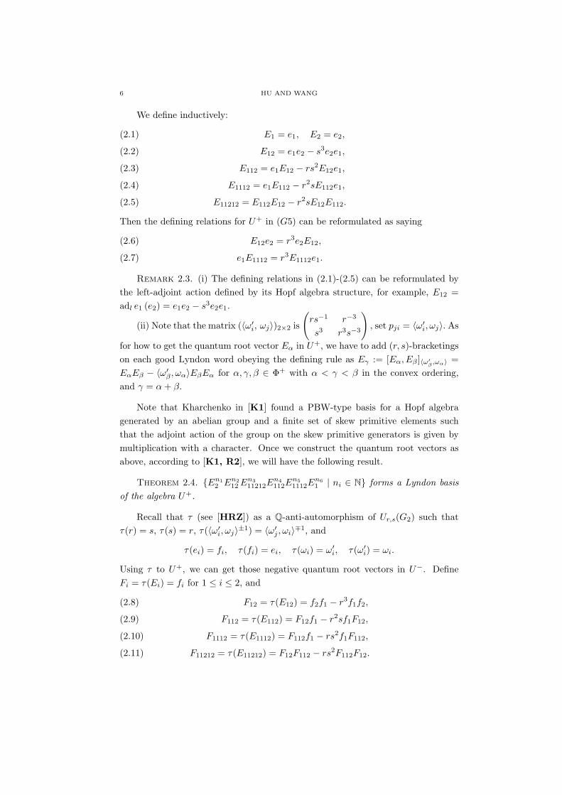
2.2. Convex PBW-type Lyndon basis. Recall that a reduced expressionof the longest element of Weyl group W for type G2 taken as

w0 = s1s2s1s2s1s2

yields a convex ordering of positive roots below:

α1, 3α1 + α2, 2α1 + α2, 3α1 + 2α2, α1 + α2, α2.

Write the positive root system Φ+ = {α1, 3α1+α2, 2α1+α2, 3α1+2α2, α1+α2, α2}.Note that the above ordering also corresponds to the standard Lyndon tree of

type G2:

d

d

t t d

d d t d´

´´

´´

´

1 1 1 2

2

2 2 1 2

With the above ordering and notation, we can make an inductive definition ofthe quantum root vectors Eα in U+ as follows. Briefly, we set Ei = Eαi , E12 =Eα1+α2 , E112 = E2α1+α2 , E1112 = E3α1+α2 , E11212 = E3α1+2α2 .

6 HU AND WANG

We define inductively:

E1 = e1, E2 = e2,(2.1)

E12 = e1e2 − s3e2e1,(2.2)

E112 = e1E12 − rs2E12e1,(2.3)

E1112 = e1E112 − r2sE112e1,(2.4)

E11212 = E112E12 − r2sE12E112.(2.5)

Then the defining relations for U+ in (G5) can be reformulated as saying

E12e2 = r3e2E12,(2.6)

e1E1112 = r3E1112e1.(2.7)

Remark 2.3. (i) The defining relations in (2.1)-(2.5) can be reformulated bythe left-adjoint action defined by its Hopf algebra structure, for example, E12 =adl e1 (e2) = e1e2 − s3e2e1.

(ii) Note that the matrix (〈ω′i, ωj〉)2×2 is

(rs−1 r−3

s3 r3s−3

), set pji = 〈ω′i, ωj〉. As

for how to get the quantum root vector Eα in U+, we have to add (r, s)-bracketingson each good Lyndon word obeying the defining rule as Eγ := [Eα, Eβ ]〈ω′β ,ωα〉 =EαEβ − 〈ω′β , ωα〉EβEα for α, γ, β ∈ Φ+ with α < γ < β in the convex ordering,and γ = α + β.

Note that Kharchenko in [K1] found a PBW-type basis for a Hopf algebragenerated by an abelian group and a finite set of skew primitive elements suchthat the adjoint action of the group on the skew primitive generators is given bymultiplication with a character. Once we construct the quantum root vectors asabove, according to [K1, R2], we will have the following result.

Theorem 2.4. {En12 En2

12 En311212E

n4112E

n51112E

n61 | ni ∈ N} forms a Lyndon basis

of the algebra U+.

Recall that τ (see [HRZ]) as a Q-anti-automorphism of Ur,s(G2) such thatτ(r) = s, τ(s) = r, τ(〈ω′i, ωj〉±1) = 〈ω′j , ωi〉∓1, and

τ(ei) = fi, τ(fi) = ei, τ(ωi) = ω′i, τ(ω′i) = ωi.

Using τ to U+, we can get those negative quantum root vectors in U−. DefineFi = τ(Ei) = fi for 1 ≤ i ≤ 2, and

F12 = τ(E12) = f2f1 − r3f1f2,(2.8)

F112 = τ(E112) = F12f1 − r2sf1F12,(2.9)

F1112 = τ(E1112) = F112f1 − rs2f1F112,(2.10)

F11212 = τ(E11212) = F12F112 − rs2F112F12.(2.11)


Corollary 2.5. {Fm11 Fm2

1112Fm3112Fm4

11212Fm512 Fm6

2 | mi ∈ N} forms a Lyndonbasis of the algebra U−.

3. Restricted two-parameter quantum groups

From now on, we restrict the parameters r and s to be roots of unity: r is aprimitive dth root of unity, s is a primitive d′th root of unity and ` is the leastcommon multiple of d and d′. We suppose that K contains a primitive `th root ofunity. We will construct a finite-dimensional Hopf algebra ur,s(G2) of dimension `16

as a quotient of Ur,s(G2) by a Hopf ideal I, which is generated by certain centralelements.

3.1. Commutation relations in U+ and central elements. We give somecommutation relations, which hold in the positive part of two-parameter quantumgroup of type G2, and the relations are actually useful for determining centralelements in this subsection and integrals in section 6.

In the following lemmas, we adopt the following notational conventions: ξ =r2 − s2 + rs, η = r2 − s2 − rs and ζ = (r3 − s3)(r + s)−1, and we will need ther, s-integers, factorials and binomial coefficients defined for positive integers i, n

and m by

[n]i :=rin − sin

ri − si, [n]1 := [n],

[n]! := [n][n− 1] · · · [2][1],[ n

m

]:=

[n]![m]![n−m]!

.

By convention [0] = 0 and [0]! = 1.

Lemma 3.1. 1 The following relations hold in U+ :(1) E112e2 = (rs)3e2E112 + r(r2−s2)E2

12;(2) E11212e2 = (r2s)3e2E11212 + r3(r−s)(r2−s2)E3

12;(3) E1112e2 = (rs2)3e2E1112 + (r2s)(r3−s3)E12E112 + rηE11212;(4) E1112E12 = (rs)3E12E1112 + rζE2

112;(5) e1E11212 = (rs)3E11212e1 + rζE2

112;(6) E1112E112 = r3E112E1112;(7) E1112E11212 = (r2s)3E11212E1112 + r3ζ(r−s)E3

112.

(8) E11212E12 = r3E12E11212;(9) E112E11212 = r3E11212E112.

Proof. (1) follows directly from (2.3), (2.6) and (2.2).

(2) follows from (2.5), (2.6) and (1).

(3): Using (2.3), we have

e1E212 = E112E12 + rs2E12E112 + (rs2)2E2

12e1.

1The proof of (6) is different from the one given in Lemma 3.7 in [HS].

8 HU AND WANG

Furthermore, using (2.4), (1) and (2.2), (2.5), we have

E1112e2 = (e1E112 − r2sE112e1)e2

= (rs)3e1e2E112 + r(r2−s2)e1E212 − r2sE112e1e2

= (rs)3(E12 + s3e2e1)E112 + r(r2−s2)e1E212 − r2sE112(E12 + s3e2e1)

= (rs)3E12E112 + (rs2)3e2e1E112 + r(r2−s2)e1E212 − r2sE112E12

− (rs2)2((rs)3e2E112 + r(r2−s2)E212)e1

= (rs)3E12E112 + (rs2)3e2e1E112 + r(r2−s2)E112E12

+ (rs)2(r2−s2)E12E112 + r3s4(r2−s2)E212e1 − r2sE112E12

+ (rs2)3e2E1112 − (rs2)3e2e1E112 − r3s4(r2−s2)E212e1

= (rs2)3e2E1112 + (r2s)(r3−s3)E12E112 + rηE11212.

(4): Using (2.2), (2.7) and (3), we have

E1112E12 = E1112(e1e2 − s3e2e1)

= r−3e1E1112e2 − s3E1112e2e1

= r−3e1((rs2)3e2E1112 + (rs)2ξE12E112 + rηE112E12)

− s3((rs2)3e2E1112 + (rs)2ξE12E112 + rηE112E12)e1

= s6e1e2E1112 + r−1s2ξe1E12E112 + r−2ηe1E112E12

− (rs3)3e2E1112e1 − r2s5ξE12E112e1 − rs3ηE112E12e1

= s6E12E1112 + r−1s2ξE2112 + s4ξE12e1E112 + r−2ηE1112E12

+ sηE112e1E12 − r2s5ξE12E112e1 − rs3ηE112E12e1

= s6E12E1112 + s4ξE12E1112 + r−1s2ξE2112 + r−2ηE1112E12 + sηE2

112,

that is,(r+s)E1112E12 = (rs)3(r+s)E12E1112 + r(r3−s3)E2

112.

Since we have assumed that r2 6= s2, this implies (4).

(5): Using (2.5), (2.4) and (2.3), we have

e1E11212 − (rs)3E11212e1 = E1112E12 − (rs)3E12E1112,

and using (4), we have the desired result.

(6): Using (2.3), (2.7) and (4), we have

E1112E112 = s3E112E1112 + r−2ζ(e1E2112 − (r2s)2E2

112e1),

on the other hand, using (2.4), we have

E1112E112 = e1E2112 − r2sE112E1112 − (r2s)2E2

112e1,

so that owing to r2 + s2 6= 0, we obtain

E1112E112 = r3E112E1112.


(7) can be proved by using (2.5), (6) and (4).

(8): It is easy to check the following relations:

e1E312 − (rs2)3E3

12e1 = E112E212 + rs2E12E11212 + r2s3(r+s)E2

12E112, (∗)

E2112e2 − (rs)6e2E

2112 = r4s3(r2−s2)E2

12E112 + r(r2−s2)E112E212, (∗∗)

E112E212 − (r2s)2E2

12E112 = E11212E12 + r2sE12E11212. (∗ ∗ ∗)Using (2.2), (5) and (2), we have

E11212E12 = E11212(e1e2 − s3e2e1)

= (rs)−3(e1E11212 − rζE2112)e2

− s3((r2s)3e2E11212 + r3(r−s)(r2−s2)E312)e1

= s−3e1((rs)3e2E11212 + (r−s)(r2−s2)E312)

− r−2s−3ζE2112e2 − (rs)3e2(e1E11212 − rζE2

112)

− (rs)3(r−s)(r2−s2)E312e1

= r3E12E11212

+ s−3(r−s)(r2−s2)(E112E212 + rs2E12E11212 + r2s3(r+s)E2

12E112)

− r−2s−3ζ(r4s3(r2−s2)E212E112 + r(r2−s2)E112E

212)

= r3E12E11212 − (rs)−1(r−s)2(E112E212 − (r2s)2E2

12E112)

+ rs−1(r−s)(r2−s2)E12E11212

= r3E12E11212 − (rs)−1(r−s)2(E11212E12 + r2sE12E11212)

+ rs−1(r−s)(r2−s2)E12E11212,

so that,

(1+r−1s−1(r−s)2)E11212E12 = (r3+rs−1(r−s)(r2−s2)− r(r−s)2)E12E11212.

Since we have assumed that r2 + s2 − rs 6= 0, this implies

E11212E12 = r3E12E11212.

(9): On the one hand, we have

E112E11212 = (e1E12 − rs2E12e1)E11212

= r−3e1E11212E12 − rs2E12e1E11212

= r−3((rs)3E11212e1 + rζE2112)E12

− rs2E12((rs)3E11212e1 + rζE2112)

= s3E11212E112 + r−2ζ(E2112E12 − (r2s)2E12E

2112),

on the other hand, we have

E2112E12 = E112E11212 + r2sE11212E112 + (r2s)2E12E

2112,

10 HU AND WANG

hence, we obtainE112E11212 = r3E11212E112,

since r2 + s2 6= 0. ¤

The main result of this subsection is the following theorem.

Theorem 3.2. E`α, F `

α (α ∈ Φ+) and ω`k − 1, (ω′k)` − 1 (k = 1, 2) are central

in Ur,s(G2).

The proof of Theorem 3.2 will be achieved through a sequence of lemmas.

Lemma 3.3. Let x, y, z be elements of a K-algebra such that yx = αxy + z forsome α ∈ K and n a natural number. Then the following assertions hold.

(1) If zx = βxz for some β(6= α) ∈ K, then yxn = αnxny + αn−βn

α−β xn−1z;

(2) If yz = βzy for some β(6= α) ∈ K, then ynx = αnxyn + αn−βn

α−β zyn−1. ¤

Lemma 3.4. For any positive integer a, the following equalities hold.(1) Ea

12e2 = r3ae2Ea12;

(2) e1Ea1112 = r3aEa

1112e1;(3) e1E

a112 = (r2s)aEa

112e1 + r2(a−1)[a]Ea−1112 E1112;

(4) e1Ea11212 = (rs)3aEa

11212e1 + r3a−2ζ[a]3Ea−111212E

2112;

(5) Ea11212e2 = (r2s)3ae2E

a11212 + r3(2a−1)(r−s)(r2−s2)[a]3E3

12Ea−111212;

(6) e1ea2 = s3aea

2e1 + [a]3ea−12 E12.

Proof. (1) & (2) follow from (2.6) and (2.7).

(3) follows from Lemma 3.3 (1), where x = E112, y = e1, z = E1112, α = r2s,β = r3, and e1E112 = E1112 + r2sE112e1, E1112E112 = r3E112E1112.

(4) follows from Lemmas 3.3 (1), 3.1 (5) & (9), where x = E11212, y = e1, z =rζE2

112, α = (rs)3, β = r6, and e1E11212 = (rs)3E11212e1+rζE2112 and E112E11212 =

r3E11212E112.

(5) follows from Lemmas 3.1 (2) & 3.3 (2), where y = E11212, x = e2, z =r3(r−s)(r2−s2)E3

12, α = (r2s)3 and β = r9.

(6) follows from Lemma 3.3 (1), together with (2.2), (2.6). ¤

Lemma 3.5. For any positive integer a, the following equalities hold.

(1)Ea112e2 = (rs)3ae2E

a112+r3(a−2)(r2−s2)

(r4s2(a−1)[a]E2

12E2112+r3sa−2[2]

[a2

]

×E12E11212E112 + [2][

a3

]E2

11212

)Ea−3

112 ;

(2) ea1e2 = s3ae2e

a1 + s2(a−1)[a]E12e

a−11 +sa−2

[a2

]E112e

a−21 +

[a3

]E1112e

a−31 ,

for a > 4;

(3) e1Ea12 = (rs2)aEa

12e1 + (rs)a−1[a]Ea−112 E112 + ra−2

[a2

]Ea−2

12 E11212;

(4) Ea1112e2 = (rs2)3ae2E

a1112 + (r2s)(rs)3(a−1)(r3−s3)[a]3E12E112E

a−11112

+ rη(rs)3(a−1)[a]3E11212Ea−11112 + r3(a−1)ζ(r−s)[2]3

[a2

]3E3

112Ea−21112.


Proof. (1): Use induction on a. If a = 1, this is Lemma 3.1 (1). UsingE112E

212 = (r2s)2E2

12E112 + r2[2]E12E11212, (2.5) and Lemma 3.1 (9), we can prove(1) to be true for a = 2, 3, 4. Suppose that (1) is true for all a ≥ 4, we obtain

Ea+1112 e2 = (rs)3aE112e2E

a112 + r3(a−2)(r2−s2)

(r4s2(a−1)[a]E112E

212E

2112

+ r3sa−2[2][a

2

]E112E12E11212E112 + [2]

[a

3

]E112E

211212

)Ea−3

112

= (rs)3(a+1)e2Ea+1112 + r(rs)3a(r2−s2)E2

12Ea112

+ r3(a−2)(r2−s2)(r8s2a[a]E2

12E3112 + r6s2a−2[2][a]E12E11212E

2112

+ r3sa−2[2][a

2

]E2

11212E112 + r8sa−1[2][a

2

]E12E11212E

2112

+ r6[2][a

3

]E2

11212E112

)Ea−3

112

= (rs)3(a+1)e2Ea+1112 + r3(a−1)(r2−s2)

(r4s2a[a+1]E2

12E2112

+ r3sa−1[2][a+12

]E12E11212E112 + [2]

[a+13

]E2

11212

)Ea−2

112

by the induction hypothesis.(2): We use induction on a. If a = 4, using the defining relations (2.2), (2.3),

(2.4), & (2.7), and a simple computation, we have

e41e2 = [4]E1112e1 + s2

[42

]E112e

21 + s6[4]E12e

31 + s12e2e

41.

Furthermore, using the induction hypothesis and (2.7), we obtain

ea+11 e2 =

[a+13

]E1112e

a−21 + sa−1

[a+12

]E112e

a−11

+ s2a[a+1]E12ea1 + s3(a+1)e2e

a+11 .

(3): We use induction on a. If a = 2, using (2.3), we have

e1E212 = E11212 + rs[2]E12E112 + (rs2)2E2

12e1.

Suppose that (3) is true for a ≥ 2, using the induction hypothesis, (2.5) and Lemma3.1 (8), we obtain

e1Ea+112 = (rs2)aEa

12e1E12 + (rs)a−1[a]Ea−112 E112E12 + ra−2

[a

2

]Ea−2

12 E11212E12

= (rs2)aEa12E112 + (rs2)a+1Ea+1

12 e1 + (rs)a−1[a]Ea−112 E11212

+ ra+1sa[a]Ea12E112 + ra+1

[a

2

]Ea−1

12 E11212

= (rs2)a+1Ea+112 e1 + (rs)a[a+1]Ea

12E112 + ra−1

[a+12

]Ea−1

12 E11212.

(4): We use induction on a. If a = 1, this is the relation in Lemma 3.1 (3).

12 HU AND WANG

Suppose that (4) is true for all a ≥ 1, using the induction hypothesis andLemma 3.1 (3), (4), (6) & (7), we obtain

Ea+11112e2 = (rs2)3a

(E1112e2

)Ea

1112

+ (r2s)(rs)3(a−1)(r3−s3)[a]3(E1112E12

)E112E

a−11112

+ rη(rs)3(a−1)[a]3(E1112E11212

)Ea−1

1112

+ r3(a−1)ζ(r−s)[2]3[a

2

]3

(E1112E

3112

)Ea−2

1112

= (rs2)3a((rs2)3e2E1112 + (r2s)(r3−s3)E12E112 + rηE11212

)Ea

1112

+ (r2s)(rs)3(a−1)(r3−s3)[a]3((rs)3E12E1112 + rζE2

112

)E112E

a−11112

+ rη(rs)3(a−1)[a]3((r2s)3E11212E1112 + r3ζ(r−s)E3

112

)Ea−1

1112

+ r3a+6ζ(r−s)[2]3[a

2

]3E3

112Ea−11112

= (rs2)3(a+1)e2Ea+11112 + (r2s)(rs)3a(r3−s3)[a+1]3E12E112E

a1112

+ rη(rs)3a[a+1]3E11212Ea1112 + r3aζ(r−s)[2]3

[a+12

]

3

E3112E

a−11112.

This completes the proof. ¤

Lemma 3.6. For any positive integer a, the following equalities hold.(1) ea

kfk = fkeak + [a]k ea−1

ks−a+1

k ωk−r−a+1k ω′k

rk−sk, 1 ≤ k ≤ 2;

(2) Ea12f1 = f1E

a12 − r2(a−1)[3][a]e2E

a−112 ω′1;

(3) Ea112f1 = f1E

a112− (rs)a−1[2]2[a]E12E

a−1112 ω′1− ra−2[2]2

[a2

]E11212E

a−2112 ω′1;

(4) Ea1112f1 = f1E

a1112 − [3][a]3E112E

a−11112ω

′1;

(5) Ea11212f1 = f1E

a11212 − r3a−2(r2−s2)[3][a]3E2

12Ea−111212ω

′1.

Proof. (1) can be easily verified by induction on a.(2), (4) & (5) follow from Lemma 3.3 (2), and the following

E12f1 = f1E12 − [3]e2ω′1,

E112f1 = f1E112 − [2]2E12ω′1,

E1112f1 = f1E1112 − [3]E112ω′1,

E11212f1 = f1E11212 − r(r2−s2)[3]E212ω

′1.

(3) can be verified by induction on a.

Ea+1112 f1 =

(E112f1

)Ea

112 − (rs)a−1[2]2[a](E112E12

)Ea−1

112 ω′1

− ra−2[2]2[a

2

] (E112E11212

)Ea−2

112 ω′1

= f1Ea+1112 − (rs)a[2]2[a+1]E12E

a112ω

′1 − ra−1[2]2

[a+12

]E11212E

a−1112 ω′1.

This completes the proof. ¤


Lemma 3.7. For any positive integer a, the following equalities hold.(1) Ea

12f2 = f2Ea12 + ω2E

a−312

(s2(a−1)E2

12e1 + sa−2[

a2

]E12E112 +

[a3

]E11212

);

(2) Ea112f2=f2E

a112+r3(a−2)(r2−s2)ω2E

a−3112

([2]

[a3

]E2

1112+r3sa−2[2][

a2

]E112×

×E1112e1 + [a]r4s2(a−1)E2112e

21

);

(3) Ea1112f2 = f2E

a1112 + r−3(a−2)(r2−s2)(r−s)[a]3ω2e

31E

a−11112;

(4) Ea11212f2 = f2E

a11212 + r(rs)3(a−1)[a]3ω2E

a−111212

(ηE1112 + rs(r3−s3)E112e1

)

+ r3(a−1)ζ(r−s)[2]3[

a2

]3ω2E

a−211212E

3112.

Proof. (1): Since E12f2 = f2E12 + ω2e1, it is easy to check the cases whena = 2, 3, 4. Using the induction hypothesis, and by Lemma 3.5 (3), we have

Ea+112 f2 = E12f2E

a12 + ω2E

a−212

(s2a+1[a]E2

12e1+sa+1[a

2

]E12E112+s3

[a

3

]E11212

)

= f2Ea+112 + ra−2ω2

(r2s2aEa

12e1+rsa−1[a]Ea−112 E112+

[a

2

]Ea−2

12 E11212

)

+ ω2Ea−212

(s2a+1[a]E2

12e1 + sa+1[a

2

]E12E112 + s3

[a

3

]E11212

)

= f2Ea+112 + ω2E

a−212

(s2a[a+1]E2

12e1+sa−1

[a+12

]E12E112

+[a+13

]E11212

).

(2): From (1), it is easy to calculate E112f2 = f2E112 + r(r2−s2)ω2e21. The

relation below is obtained by Lemma 3.4 (3),

e21E

a112 = r4a−6Ea−2

112

([2]

[a

2

]E2

1112 + r4sa−1[2][a]E112E1112e1 + r6s2aE2112e

21

).

For a ≥ 1, we have by induction on a,

Ea+1112 f2 =

(E112f2

)Ea

112 + r3(a−1)s3(r2−s2)ω2Ea−2112

([2]

[a

3

]E2

1112

+ r3sa−2[2][a

2

]E112E1112e1 + r4s2(a−1)[a]E2

112e21

)

= f2Ea+1112 + r(r2−s2)r4a−6ω2E

a−2112

([2]

[a

2

]E2

1112

+ r4sa−1[2][a]E112E1112e1 + r6s2aE2112e

21

)

+ r3(a−1)s3(r2−s2)ω2Ea−2112

([2]

[a

3

]E2

1112

+ r3sa−2[2][a

2

]E112E1112e1 + r4s2(a−1)[a]E2

112e21

)

= f2Ea+1112 + r3(a−1)(r2−s2)ω2E

a−2112

([2]

[a+13

]E2

1112

+ r3sa−1[2][a+12

]E112E1112e1 + r4s2a[a+1]E2

112e21

).

(3): We consider the case for a = 1. It follows from (2) that

E1112f2 = f2E1112 + r3(r2−s2)(r−s)ω2e31. (∗)

14 HU AND WANG

So by (∗) and Lemma 3.3 (2), we can easily get (3).(4): If a = 1, we have

E11212f2 = f2E11212 + rηω2E1112 + r2s(r3−s3)ω2E112e1

by using (1) and (2). The following relation holds by Lemma 3.3 (1):

E1112Ea11212 = (r2s)3aEa

11212E1112 + r3(2a−1)ζ(r−s)[a]3Ea−111212E

3112. (∗∗)

So (4) can be derived easily from (∗∗) and Lemma 3.4 (4) by induction on a.The proof is complete. ¤

Proof of Theorem 3.2. We know from Lemmas 3.4, 3.5, 3.6, 3.7 that theelements E`

1, E`1112, E`

112, E`11212, E`

12, E`2 are central in Ur,s(G2). Applying τ to

Eα (α ∈ Φ), we see that F `1 , F `

1112, F `112, F `

11212, F `12, F `

2 are also central. It is easyto see that ω`

k − 1, (ω′k)` − 1 (k = 1, 2) are central too. ¤

Remark 3.8. If ` = 3`′, then the elements E`′1112, F

`′1112, ω`′

k −1 and (ω′k)`′−1(k = 1, 2) are central in Ur,s(G2).

3.2. Restricted two-parameter quantum groups. From now on we willassume that ` is coprime to 3.

Definition 3.9. The restricted two-parameter quantum group is the quotient

ur,s(G2) := Ur,s(G2)/I,

where I denotes the ideal of Ur,s(G2) generated by all elements E`α, F `

α (α ∈ Φ+)and ω`

k − 1, (ω′k)` − 1 (1 ≤ k ≤ 2).

By Theorem 2.4 and Corollary 2.5, ur,s(so2n+1) is an algebra of dimension `16

with linear basis

(3.1) Ec12 Ec2

12Ec311212E

c4112E

c51112E

c61 ωb1

1 ωb22 (ω′1)

b′1(ω′2)b′2F

c′11 F

c′21112F

c′3112F

c′411212F

c′512F

c′62

where all powers range between 0 and `− 1.The remainder of this section is devoted to proving that ur,s(G2) is a finite-

dimensional Hopf algebra.First note that the generators of I are contained in the kernel of the counit ε,

and so I is as well. Because the coproduct ∆ is an algebra homomorphism, andthe antipode S is an algebra antihomomorphism, it suffices to show that ∆(x) ∈I ⊗U + U ⊗ I and S(x) ∈ I for each generator x ∈ I. To accomplish this, we relyon the following computations:

∆(ω`k − 1) = ω`

k ⊗ ω`k − 1⊗ 1

= (ω`k − 1)⊗ ω`

k + 1⊗ (ω`k − 1) ∈ I ⊗ U + U ⊗ I,


and S(ω`k − 1) = −ω−`

k (ω`k − 1) ∈ I. The argument for (ω′k)` − 1 is similar. In

determining ∆(x) for each generator x ∈ I, we adopt the notation below

ω12 = ω1ω2, ω112 = ω21ω2, ω1112 = ω3

1ω2, ω11212 = ω31ω2

2 .

Some simple computations give rise to the following

Lemma 3.10. (1) ∆(E12) = E12 ⊗ 1 + ω12 ⊗ E12 + (r3−s3)ω2e1 ⊗ e2;(2) ∆(E112) = E112⊗ 1+ω112⊗E112 +(r+s)(r2−s2)ω12e1⊗E12 + r(r2−s2)×

(r3−s3)ω2e21 ⊗ e2;

(3) ∆(E1112) = E1112⊗ 1 + ω1112⊗E1112 + (r3−s3)ω112e1⊗E112 + r(r2−s2)×(r3−s3)ω12e

21 ⊗ E12 + r3(r−s)(r2−s2)(r3−s3)ω2e

31 ⊗ e2;

(4) ∆(E11212) = E11212 ⊗ 1 + ω11212 ⊗E11212 + r(r2−s2)(r3−s3)ω212e1 ⊗E2

12 +r(r2−s2)(r3−s3)2ω12ω2e

21 ⊗ E12e2 + (r3−s3)ω12E112 ⊗ E12 + r6(r−s)(r2−s2) ×

(r3−s3)2ω22e3

1 ⊗ e22 + r(r3−s3)ω2((r2−s2−rs)E1112 + rs(r3−s3)E112e1)⊗ e2. ¤

Lemma 3.11. ∆(E`α) ∈ I ⊗ U + U ⊗ I, for α ∈ Φ+.

Proof. Note that

∆(eni ) =

n∑

j=0

(n

j

)

ris−1i

en−ji ωj

i ⊗ eji

has a ris−1i -binomial expansion 2 since (ωi⊗ ei)(ei⊗ 1) = ris

−1i (ei⊗ 1)(ωi⊗ ei). So

we have ∆(e`i) = e`

i ⊗ 1 + ω`i ⊗ e`

i ∈ I ⊗ U + U ⊗ I, since r and s are primitive `throot of unity, and

(`j

)ris

−1i

= 0 for 0 < j < `.

Note that ∆(E`12) = (E12 ⊗ 1 + (r3 − s3)ω2e1 ⊗ e2)` + ω`

12 ⊗ E`12, because of

(ω12⊗E12)(E12⊗1+(r3−s3)ω2e1⊗e2) = rs−1(E12⊗1+(r3−s3)ω2e1⊗e2)(ω12⊗E12).

we get ∆(E`12) = E`

12⊗ 1 + r3`(`−1)

2 (r3−s3)`ω`2e

`1⊗ e`

2 + ω`12⊗E`

12 ∈ I ⊗U + U ⊗I,as r, s are primitive `th root of unity, and (E12 + ω2e1)` = E`

12 + r3`(`−1)

2 ω`2e

`1. In

a similar way, we have ∆(E`112),∆(E`

1112),∆(E`11212) are in I ⊗ U + U ⊗ I. ¤

Applying the antipode property to ∆(E`α), α ∈ Φ+, we can obtain S(E`

α) ∈I ⊗ U + U ⊗ I. Using τ , we find that ∆(F `

α) ∈ I ⊗ U + U ⊗ I for α ∈ Φ+. Hence,I is a Hopf ideal, and ur,s(G2) is a finite-dimensional Hopf algebra. Then we have

Theorem 3.12. I is a Hopf ideal of Ur,s(G2), so that ur,s(G2) is a finite-dimensional Hopf algebra. ¤

2We set

(n) := (n)rs−1 :=rns−n − 1

rs−1 − 1, (n)! := (n)(n− 1) · · · (2)(1),

( n

m

):=

(n)!

(m)!(n−m)!.

By convention (0) = 0 and (0)! = 1.

16 HU AND WANG

4. Isomorphisms of ur,s(G2)

Write u = ur,s = ur,s(G2). Let G denote the group generated by ωi, ω′i (i = 1, 2)in the restricted quantum group u. Define linear subspace ak of u by

a0 = KG, a1 = KG +2∑

i=1

(KeiG +KfiG),

ak = (a1)k for k ≥ 1.

(4.1)

Note that 1 ∈ a0, ∆(a0) ⊆ a0 ⊗ a0, a1 generates u as an algebra, and ∆(a1) ⊆a1⊗a0 +a0⊗a1. By [M], {ak} is a coalgebra filtration of u and u0 ⊆ a0, where thecoradical u0 of u is the sum of all the simple subcoalgebras of u. Clearly, a0 ⊆ u0

as well, and so u0 = KG. This implies that u is pointed, that is, every simplesubcoalgebra of u is one-dimensional.

Let b be the Hopf subalgebra of u = ur,s(G2) generated by ei, ω±1i (i = 1, 2),

and b′ the Hopf subalgebra generated by fi, (ω′i)±1 (i = 1, 2). The same argument

shows that b and b′ are pointed as well. Thus, we have

Proposition 4.1. The restricted two-parameter quantum group ur,s(G2) is apointed Hopf algebra, as are its subalgebras b and b′.

Lemma 5.5.1 in [M] indicates that ak ⊆ uk for all k, where {uk} is the coradicalfiltration of u defined inductively by uk = ∆−1(u × uk−1 + u0 × u). In particular,a1 ⊆ u1. By Theorem 5.4.1 in [M], as u is pointed, u1 is spanned by the set ofgroup-like elements G together with all the skew-primitive elements of u. We claimthat under the additional hypothesis of the Lemma below, u1 = a1. That is, eachskew-primitive element of u is a linear combination of elements of G, of eiG, andof fiG (i = 1, 2).

The following Lemma gives a precise description of u1.

Lemma 4.2. Assume that rs−1 is a primitive `th root of unity. Then

u1 = KG +2∑

i=1

(KeiG +KfiG).

Given two group-like elements g, h in a Hopf algebra H, let Pg,h(H) denote theset of skew-primitive elements of H given by

Pg,h(H) = {x ∈ H | ∆(x) = x⊗ g + h⊗ x}.We want to compute P1,σ(ur,s) and Pσ,1(ur,s) for σ ∈ G.

Lemma 4.3. Assume that rs−1 is a primitive `th root of unity. Then we have(1) P1,ωi(ur,s) = K(1− ωi) +Kei, P1,ω′−1

i(ur,s) = K(1− ω′−1

i ) +Kfiω′−1i ,

P1,σ(ur,s) = K(1− σ) if σ 6∈ {ωi, ω′−1i | i = 1, 2 };

(2) Pω′i,1(ur,s) = K(1− ω′i) +Kfi, Pω−1i ,1(ur,s) = K(1− ω−1

i ) +Keiω−1i ,

Pσ,1(ur,s) = K(1− σ) if σ 6∈ {ω′i, ω−1i | i = 1, 2 }.


Proof. (1) Assuming rs−1 is a primitive `th root of unity, we have

KG +∑

g,h∈G

Pg,h(ur,s) = KG +2∑

i=1

(KeiG +KfiG).

Thus, any x ∈ P1,σ(ur,s) (where σ ∈ G) may be written as a linear combination

x =∑

g∈G

γgg +∑

g∈G

2∑

i=1

αi,geig +∑

g∈G

2∑

i=1

βi,gfig,

where γg, αi,g and βi,g are scalars. Comparing ∆(x) = x ⊗ 1 + σ ⊗ x with thecoproduct of the right side, which is

∑

g∈G

γgg ⊗ g +∑

g∈G

2∑

i=1

αi,g(eig ⊗ g + ωig ⊗ eig) +∑

g∈G

2∑

i=1

βi,g(g ⊗ fig + fig ⊗ ω′ig),

we obtain βi,g = 0 for all i and g 6= ω′−1i , and αi,g = 0 for all g 6= 1. A further

comparison of the group-like components yields γσ = −γ1 and γg = 0 for all g 6=1, σ. Finally, comparing ∆(x) with ∆(γ1(1−σ)+

2∑i=1

αi,1ei+2∑

i=1

βi,ω′−1i

fiω′−1i ) yields

αi,1 = 0 for all i when σ /∈ {ω1, ω2}, and βi,ω′−1i

= 0 for all i when σ /∈ {ω′−11 , ω′−1

2 }.(i) When σ = ωi for some i, we have αj,1 = 0 for all j 6= i; and βj,ω′−1

j= 0 for

all j. So x = γ1(1− ωi) + αi,1ei.(ii) When σ = ω′−1

i for some i, we have βj,ω′−1j

= 0 for all j 6= i; and αj,1 = 0

for all j. So x = γ1(1− ω′−1i ) + βi,ω′−1

ifiω

′−1i . Thus

P1,ωi(ur,s) = K(1− ωi) +Kei, 1 ≤ i ≤ 2,

P1,ω′−1i

(ur,s) = K(1− ω′−1i ) +Kfiω

′−1i , 1 ≤ i ≤ 2,

P1,σ(ur,s) = K(1− σ), if σ 6∈ {ωi, ω′−1i }, for any i.

Similarly, we get (2). ¤

Remark 4.4. It should be mentioned that the description of the set of left(right) skew-primitive elements of ur,s(sln) (see formulae (3.6) & (3.7) in [BW3])is not complete. This led to many families of isomorphisms of ur,s(sln) undiscovered,while in the second part of the proof of Theorem 5.4 in [HW2], authors describedexplicitly all of the Hopf algebra isomorphisms of ur,s(sln) (see Theorem 5.5 in[HW2]).

Theorem 4.5. Assume that rs−1 and r′s′−1 are primitive `th roots of unitywith ` 6= 3, 4, and ζ is a 3rd root of unity. Then ϕ : ur,s

∼= ur′,s′ as Hopf algebrasif and only if either (i) (r′, s′) = ζ(r, s), ϕ is a diagonal isomorphism: ϕ(ωi) = ωi,ϕ(ω′i) = ω′i, ϕ(ei) = aiei, ϕ(fi) = ζδi,1a−1

i fi (ai ∈ K∗); or (ii) (r′, s′) = ζ(s, r),ϕ(ωi) = ω′−1

i , ϕ(ω′i) = ω−1i , ϕ(ei) = aifiω

′−1i , ϕ(fi) = ζδi,1a−1

i ω−1i ei (ai ∈ K∗).

18 HU AND WANG

Proof. Suppose ϕ : ur,s −→ ur′,s′ is a Hopf algebra isomorphism. Writeei, fi, ωi, ω′i to distinguish the generators of ur′,s′ . Because

∆(ϕ(ei)) = (ϕ⊗ ϕ)(∆(ei)) = ϕ(ei)⊗ 1 + ϕ(ωi)⊗ ϕ(ei),

we have ϕ(ei) ∈ P1,ϕ(ωi)(ur′,s′) for i = 1, 2. As ϕ is an isomorphism, ϕ(ωi) ∈ KG.Lemma 4.3 (1) implies that ϕ(ωi) ∈ { ωj , ω′−1

j | j = 1, 2 }, that is, case (i): Fori = 1, 2, we have ϕ(ωi) = ωji

for some ji, and ϕ(ei) = α(1− ωji) + βeji

(α, β ∈ K);case (ii): For i = 1, 2, we have ϕ(ωi) = ω′−1

jifor some ji, and ϕ(ei) = α′(1 −

ω′−1ji

) + β′fji ω′−1ji

(α′, β′ ∈ K); case (iii): ϕ(ω1) = ωj1 , but ϕ(ω2) = ω′−1j2

; case(iv): ϕ(ω1) = ω′−1

j1, but ϕ(ω2) = ωj2 .

Case (i): In this case, we claim ϕ(ωi) = ωi. Otherwise, if ϕ(ω1) = ω2 andϕ(ω2) = ω1. Applying ϕ to relation ω1e1 = rs−1e1ω1 yields

ϕ(ω1)ϕ(e1) = rs−1ϕ(e1)ϕ(ω1),

ω2(α(1− ω2) + βe2) = rs−1(α(1− ω2) + βe2)ω2.

As r 6= s, this forces α to be 0, so that ϕ(e1) = βe2 for some β 6= 0. Moreover,because ω2e2 = r′2s

′−12 e2ω2, it follows that r′3s′−3 = rs−1.

Applying ϕ to relation ω1e2 = s3e2ω1, we get ϕ(ω1)ϕ(e2) = s3ϕ(e2)ϕ(ω1),i.e., ω2e1 = s3e1ω1. But ω2e1 = r′−3e1ω1 in ur′,s′ . So r′3 = s−3. Similarly, toω2e1 = r−3e1ω2 to get s′−3 = r3. Thereby, it follows from r′3s′−3 = rs−1 thatr2 = s2, which contradicts the assumption. So we proved ϕ(ωi) = ωi. Similarly, wehave ϕ(ω′i) = ω′i.

Furthermore, applying ϕ to relations ωiej = 〈ω′j , ωi〉ejωi for i, j ∈ {1, 2}, we get〈ω′j , ωi〉 = 〈ω′j , ωi〉 for i, j ∈ {1, 2}, i.e., r′3s′−3 = r3s−3, r′s′−1 = rs−1, r′−3 = r−3

and s′3 = s3. Hence, (r′, s′) = ζ(r, s), where ζ is a 3rd root of unity. As ϕ preservesrelation (G4), ϕ(ei) = aiei and ϕ(fi) = ζδi,1a−1

i fi (ai ∈ K∗), that is, ϕ is a diagonalisomorphism.

Case (ii): Since ϕ(ωi) = ω′−1ji

for some ji, and ϕ(ei) = α′(1− ω′−1ji

)+β′fjiω′−1

ji.

In fact, we have ϕ(ei) = β′fjiω′−1

ji(applying ϕ to relation ωiei = ris

−1i eiωi to get

α′ = 0). We claim ϕ(ωi) = ω′−1i . In fact, if ϕ(ω1) = ω′−1

2 and ϕ(ω2) = ω′−11 , then

ϕ(e1) = a1f2ω′−12 and ϕ(e2) = a2f1ω

′−11 . Using ϕ to relation ω1e1 = rs−1e1ω1, we

get rs−1 = (r′3s′−3)−1; to relation ω2e1 = r−3e1ω2 to get r−3 = r′3, to relationω1e2 = s3e2ω1 to get s3 = s′−3. So we have (rs−1)2 = 1. This contradicts theassumption. Hence, ϕ(ωi) = ω′−1

i , ϕ(ω′i) = ω−1i , ϕ(ei) = aifiω

′−1i , where ai ∈ K∗.

Using ϕ to relation ω1e1 = rs−1e1ω1, we get rs−1 = (r′s′−1)−1; to relationω1e2 = s3e2ω1 to get s3 = r′3; to relation ω2e1 = r−3e1ω2 to get r−3 = s′−3. So wehave (r′, s′) = ζ(s, r), where ζ is a 3rd root of unity. In order to ϕ preserve relation(G4), one has to take ϕ(fi) = ζδi,1a−1

i ω−1i ei, where ai ∈ K∗. Besides, we can easily

check that such a ϕ does preserve all of the Serre relations (G5)—(G6).


Case (iii): We claim that this case is impossible. First, we assume that ϕ(ω1) =ω1 and ϕ(ω2) = ω′−1

2 . Then we have ϕ(e1) = a1e1, ϕ(e2) = a2f2ω′−12 , where

a1, a2 ∈ K∗. Using ϕ to relation ω1e2 = s3e2ω1, we get s3 = s′−3; to relationω2e1 = r−3e1ω2 to get r−3 = s′3. So we get r3 = s3. This is a contradiction.

Next, we assume that ϕ(ω1) = ω2, and ϕ(ω2) = ω′−11 . Then we have ϕ(e1) =

a1e2, ϕ(e2) = a2f1ω′−11 , where a1, a2 ∈ K∗. Using ϕ to relation ω1e2 = s3e2ω1, we

get s3 = r′3; to relation ω2e1 = r−3e1ω2 to get r−3 = r′−3. So we have r3 = s3,which is contrary to the condition.

Case (iv): Similarly to case (iii), it is also impossible.So we complete the proof. ¤

5. ur,s(G2) is a Drinfel’d double

We will show that u ∼= D(b) under a few assumptions. Let θ be a primitive `throot of unity in K, and write r = θy, s = θz.

Lemma 5.1. Assume that (3(y2 + z2 + yz), `) = 1 and rs−1 is a primitive `throot of unity. Then (b′)coop ∼= b∗ as Hopf algebras.

Proof. Define γj , ηj (j = 1, 2) of b∗ as follows: The γj ’s are algebra homo-morphisms with γj(ωi) = 〈ω′j , ωi〉 and γj(ei) = 0 for i = 1, 2. So they are group-likeelements in b∗. Let ηj =

∑g∈G(b)

(ejg)∗, where G(b) is the group generated by ω1, ω2

and the asterisk denotes the dual basis element relative to the PBW-basis of b. Theisomorphism φ : (b′)coop −→ b∗ is then defined by

φ(ω′j) = γj and φ(fj) = ηj .

We have to check that φ is a Hopf algebra homomorphism and it is a bijection.First, we observe that the γj ’s are invertible elements in b∗ that commute with

one another and γ`j = 1. Note that η`

j = 0, as it is 0 on any basis element of b. Wecalculate γjηiγ

−1j : It is nonzero only on basis elements of the form eiω

k11 ωk2

2 , andon such an element it takes the value

(γj ⊗ ηi ⊗ γ−1j )((ei ⊗ 1⊗ 1 + ωi ⊗ ei ⊗ 1 + ωi ⊗ ωi ⊗ ei)(ωk1

1 ωk22 )⊗3)

= γj(ωiωk11 ωk2

2 )ηi(eiωk11 ωk2

2 )γ−1j (ωk1

1 ωk22 )

= γj(ωi) = 〈ω′j , ωi〉.

Thus we have γjηiγ−1j = 〈ω′j , ωi〉ηi, which corresponds to relation (G3) for b′. Next,

we check relation (G6): we compute

(η22η1)(e2

2e1)

= (η2 ⊗ η2 ⊗ η1)((e2 ⊗ 1⊗ 1 + ω2 ⊗ e2 ⊗ 1 + ω2 ⊗ ω2 ⊗ e2)2

× (e1 ⊗ 1⊗ 1 + ω1 ⊗ e1 ⊗ 1 + ω1 ⊗ ω1 ⊗ e1))

20 HU AND WANG

= (η2 ⊗ η2 ⊗ η1)(e2ω2ω1 ⊗ e2ω1 ⊗ e1 + ω2e2ω1 ⊗ e2ω1 ⊗ e1)

= (η2 ⊗ η2 ⊗ η1)((1 + r3s−3)e2ω2ω1 ⊗ e2ω1 ⊗ e1) = 1 + r3s−3,

and similarly, (η22η1)(e2E12) = 0. Thus, for any k1, k2, we have (η2

2η1)(e22 e1ω

k11 ωk2

2 )= 1 + r3s−3 and (η2

2η1)(e2E12ωk11 ωk2

2 ) = 0. On all other basis elements, η22η1 is 0.

Therefore, we have

η22η1 =

∑

g∈G

(1 + r3s−3)(e22e1g)∗. (∗)

Similarly, we calculate

(η2η1η2)(e22e1)

= (η2 ⊗ η1 ⊗ η2)(e2ω2ω1 ⊗ ω2e1 ⊗ e2 + ω2e2ω1 ⊗ ω2e1 ⊗ e2)

= r−3 + s−3,

(η2η1η2)(e2E12)

= (η2η1η2)(e2e1e2 − s3e22e1)

= (η2 ⊗ η1 ⊗ η2)(ω2ω1e2 ⊗ ω2e1 ⊗ e2 + e2ω1ω2 ⊗ e1ω2 ⊗ e2)− 1− r−3s3

= 1− r−3s3.

So we have

η2η1η2 =∑

g∈G

((r−3 + s−3)(e22e1g)∗ + (1− r−3s3)(e2E12g)∗). (∗∗)

We compute

(η1η22)(e2

2e1) = r−3(r−3 + s−3),

(η1η22)(e2E12) = s3(s−6 − r−6).

So we have

η1η22 =

∑

g∈G

(r−3(r−3 + s−3)(e22e1g)∗ + s3(s−6 − r−6)(e2E12g)∗). (∗ ∗ ∗)

We use the above results in (∗)—(∗ ∗ ∗) to establish the relation

r3s3η1η22 − (r3 + s3)η2η1η2 + η2

2η1 = 0.

Similarly, it is easy to verify that

η2η41 − (r+s)(r2 + s2) η1η2η

31 + rs(r2 + s2)(r2 + rs + s2) η2

1η2η21

− (rs)3(r + s)(r2 + s2) η31η2η1 + (rs)6 η4

1η2 = 0.

Therefore, φ is an algebra homomorphism.Now we will check that φ preserves coproducts. We have already seen that γi

is a group-like element in b∗. We calculate

∆(ηi)(eiωj11 ωj2

2 ⊗ ωk11 ωk2

2 ) = ηi(eiωj1+k11 ωj2+k2

2 ) = 1,

∆(ηi)(ωj11 ωj2

2 ⊗ eiωk11 ωk2

2 ) = ηi(ωj11 ωj2

2 eiωk11 ωk2

2 ) = 〈ω′i, ω1〉j1〈ω′i, ω2〉j2 .


These are the only basis elements of b⊗ b on which ∆(ηi) is nonzero. As a conse-quence, we have

(ηi ⊗ 1 + γi ⊗ ηi)(eiωj11 ωj2

2 ⊗ ωk11 ωk2

2 ) = 1,

(ηi ⊗ 1 + γi ⊗ ηi)(ωj11 ωj2

2 ⊗ eiωk11 ωk2

2 ) = 〈ω′i, ω1〉j1〈ω′i, ω2〉j2 .

So ∆(ηi) = ηi ⊗ 1 + γi ⊗ ηi. This proves that φ is a Hopf algebra homomorphism.Finally, we prove that φ is bijective. As b∗ and (b′)coop have the same dimen-

sion, it suffices to show that φ is injective. By [M], we need only show that φ|(b′)coop1

is injective. Lemma 4.2 yields (b′)coop1 = KG(b′) +

∑2i=1KfiG(b′), where G(b′) is

the group generated by ω′1, ω′2. First, we claim that

(5.1) spanK{γk11 γk2

2 | 0 ≤ ki < ` } = spanK{(ωk11 ωk2

2 )∗ | 0 ≤ ki < ` }.

This is equivalent to the statement that the γk11 γk2

2 ’s span the space of charactersover K of the finite group Z/`Z×Z/`Z generated by ω1, ω2. We have assumed thatK contains a primitive `th root of unity. Therefore, the irreducible characters ofthis group are the functions χi1,i2 given by χi1,i2(ω

k11 ωk2

2 ) = θi1k1+i2k2 , where θ isa primitive `th root of unity in K. Note that γ1 = χy−z,−3y, γ2 = χ3z,3(y−z). Wemust show that, given i1, i2, there are k1, k2 such that χi1,i2 = γk1

1 γk22 , which is

equivalent to the existence of a solution to the matrix equation AK = I in Z/`Z

(as these are powers of θ), where A =

(y − z 3z

−3y 3(y − z)

), K is the transpose of

(k1, k2) and I is the transpose of (i1, i2). The determinant of the coefficient matrixA is 3(y2 + z2 + yz), which is invertible in Z/`Z by the hypothesis in the Lemma.Therefore (5.1) holds. In particular, this implies that the matrix

(5.2)((γk1

1 γk22 )(ωj1

1 ωj22 )

)k×j

is invertible, and that φ is bijection on group-like elements.Next we will show for each i (i = 1, 2) that the following matrix is invertible:

(5.3)((ηiγ

k11 γk2

2 )(eiωj11 ωj2

2 ))k×j

This will complete the proof that φ is injective on (b′)coop1 , as desired. We will show

that the matrix is block upper-triangular. Each matrix entry is

(ηi ⊗ γk11 γk2

2 )(∆(ei)∆(ωj11 ωj2

2 ))

= (ηi ⊗ γk11 γk2

2 )(eiωj11 ωj2

2 ⊗ ωj11 ωj2

2 ).

Thus, (5.3) is precisely the invertible matrix (5.2). ¤

Recall that the Drinfel’d double D(b) of the finite-dimensional Hopf algebrab is a Hopf algebra whose underlying coalgebra is b ⊗ (b∗)coop (that is, the vectorspace b⊗(b∗)coop with the tensor product coalgebra structure). As an algebra, D(b)

22 HU AND WANG

contains the subalgebras b⊗ 1 ∼= b and 1⊗ b∗ ∼= b∗, and if a ∈ b and b ∈ (b∗)coop,then (a⊗ 1)(1⊗ b) = a⊗ b and

(1⊗ b)(a⊗ 1) =∑

b(1)(S−1a(1))b(3)(a(3))a(2) ⊗ b(2),

where S−1 is the composition inverse of the antipode S for b.

Theorem 5.2. Assume that (3(y2 + z2 + yz), `) = 1. Then D(b) ∼= ur,s(G2) asHopf algebras.

Proof. We denote the image ei ⊗ 1 of ei in D(b) by ei, and similarly for ωi,ηi and γi. Define ψ : D(b) → ur,s(G2) on the generators by

ψ(ei) = ei, ψ(ηi) = (si − ri)fi,

ψ(ω±1i ) = ω±1

i , ψ(γ±1i ) = (ω′i)

±1.

Then the proof is the same as that of Theorem 6.2 in [HW2]. ¤

6. Integrals and ribbon elements

Integrals play a basic role in the structure theory of finite dimensional Hopfalgebras H and their duals H∗. In this section, we compute the left and rightintegrals in the Borel subalgebra b of ur,s(G2) and the distinguished group-likeelements of b and b∗. Furthermore, we use this information to determine thatur,s(G2) has a ribbon element when ur,s(G2) ∼= D(b).

Let H be a finite-dimensional Hopf algebra. An element y ∈ H is a left integral(resp. right integral) if ay = ε(a)y (resp. ya = ε(a)y) for all a ∈ H. The left (resp.right) integrals form a one-dimensional ideal

∫ l

H(resp.

∫ r

H) of H, and SH(

∫ r

H) =

∫ l

H

under the antipode SH of H.When y 6= 0 is a left integral of H, there exists a unique group-like element γ

in the dual algebra H∗ (the so-called distinguished group-like element of H∗) suchthat ya = γ(a)y. If we had begun instead with a right integral y′ ∈ H, then wewould have ay′ = γ−1(a)y′. This is an easy consequence of the fact that group-likeelements are invertible, and can be found in [[M], p.22].

Now if λ 6= 0 is right integral of H∗, then there exists a unique group-likeelement g of H (the distinguished group-like element of H) such that ξλ = ξ(g)λfor all ξ ∈ H∗. The algebra H is unimodular (i.e.,

∫ l

H=

∫ r

H) if and only if γ = ε;

and the dual algebra H∗ is unimodular if and only if g = 1.The left and right H∗-module actions on H are given by

ξ ⇀ a =∑

a(1)ξ(a(2)), a ↼ ξ =∑

ξ(a(1))a(2)

for all ξ ∈ H∗ and a ∈ H. In particular, ε ⇀ a = a = a ↼ ε for all a ∈ H.Radford [R] found a remarkable expression relating the antipode, the distinguishedgroup-like elements γ and g, and the H∗-action:

S4(a) = g(γ ⇀ a ↼ γ−1)g−1, for all a ∈ H.


This formula is crucial in [KR], where Kauffman and Radford determine a necessaryand sufficient condition for a Drinfel’d double of a Hopf algebra to have a ribbonelement.

A finite-dimensional Hopf algebra H is quasitriangular if there exists an invert-ible element R =

∑xi ⊗ yi in H ⊗H such that ∆op(a)R = R∆(a) for all a ∈ H,

and R satisfies the relations (∆ ⊗ id)R = R1,3R2,3, (id ⊗ ∆)R = R1,3R1,2, whereR1,2 =

∑xi ⊗ yi ⊗ 1, R1,3 =

∑xi ⊗ 1 ⊗ yi, and R2,3 =

∑1 ⊗ xi ⊗ yi. Suppose

u =∑

S(yi)xi. Then c = uS(u) is central in H and is referred to as the Casimirelement.

An element v ∈ H is a quasi-ribbon element of quasitriangular Hopf algebra(H, R) if

(i) v2 = c, (ii) S(v) = v, (iii) ε(v) = v, (iv) ∆(v) = (R2,1R1,2)−1(v ⊗ v),

where R2,1 =∑

yi ⊗ xi and R1,2 = R. If moreover v is central in H, then v

is a ribbon element, and (H, R, v) is said to be a ribbon Hopf algebra. Ribbonelements provide an effective means of constructing invariants of knots and links(see [KR, RT1, RT2, RTF]). The Drinfel’d double D(A) of a finite-dimensionalHopf algebra A is quasitriangular, and Kauffman and Radford have provided asimple criterion for D(A) to have a ribbon element in [KR].

Theorem 6.1. Assume that A is a finite-dimensional Hopf algebra, and let g

and γ be the distinguished group-like elements of A and A∗ respectively. Then(i) (D(A), R) has a quasi-ribbon element if and only if there exist group-like

elements h ∈ A, δ ∈ A∗ such that h2 = g and δ2 = γ.(ii) (D(A), R) has a ribbon element if and only if there exist h and δ as in (i)

such thatS2(a) = h(δ ⇀ a ↼ δ−1)h−1, for all a ∈ A.

Next we compute a left integral and a right integral in b.

Proposition 6.2. Let t =2∏

i=1

(1+ωi+· · ·+ω`−1i ) and x = E`−1

2 E`−112 E`−1

11212E`−1112

E`−11112E

`−11 . Then y = tx and y′ = xt are respectively a left integral and a right

integral in b.

Proof. To prove y = tx is a left integral in b, we need to show that by = ε(b)yfor all b ∈ b. It suffices to show this for the generators ωk and ek for k = 1, 2, asthe counit ε is an algebra homomorphism.

Observe that ωkt = t = ε(ωk)t for all k = 1, 2, as the ωi’s commute andωk(1+ωk + · · ·+ω`−1

k ) = 1+ωk + · · ·+ω`−1k . From that, the relation ωky = ε(ωk)y

is clear for all k.

Next we compute eky. By a simple calculation, we get ekt =2∏

i=1

(1+〈ω′k, ωi〉−1ωi

+ · · ·+ 〈ω′k, ωi〉−(`−1)ω`−1i )ek. So it suffices to check that ekx = 0 = ε(ek)x.

24 HU AND WANG

Note that e2x = 0, we want to show that e1 can be moved across the termsE`−1

2 E`−112 E`−1

11212 E`−1112 E`−1

1112 next to E`−11 . We have

e1E`−12 E`−1

12 E`−111212E

`−1112 E`−1

1112

= s3(`−1)E`−12 e1E

`−112 E`−1

11212E`−1112 E`−1

1112

= r`−1s5(`−1)E`−12 E`−1

12 e1E`−111212E

`−1112 E`−1

1112

= r4(`−1)s8(`−1)E`−12 E`−1

12 E`−111212e1E

`−1112 E`−1

1112

= r6(`−1)s9(`−1)E`−12 E`−1

12 E`−111212E

`−1112 e1E

`−11112

= r9(`−1)s9(`−1)E`−12 E`−1

12 E`−111212E

`−1112 E`−1

1112e1,

where we get the first ”=” by using Lemma 3.4 (6), the second by using Lemmas3.5 (3) & 3.1 (9), the third by using Lemma 3.4 (4), the forth by using Lemma 3.4(3) and the last by using Lemma 3.4 (2). Thus, we have e1x = 0, which implies thedesired conclusion that y is a left integral in b.

To prove that y′ = xt is a right integral in b, it suffices to show that xej = 0.Note that xe1 = 0. By a similar argument and Lemma 3.5 (2), (4), (1), Lemma 3.4(5), (1) and Lemma 3.1 (4), (6), (8) and (9), together with (2.5) & (2.6), we canmove e2 to the left until it is next to E`−1

2 , which gives zero. ¤

A finite-dimensional Hopf algebra H is semisimple if and only if ε(∫ l

H) 6= 0 if

and only if ε(∫ r

H) 6= 0. For the algebra b above, y gives a basis for

∫ l

band y′ a basis

for∫ r

b. As ε(y) = 0 = ε(y′), we have

Proposition 6.3. The Hopf algebra b is not semisimple. ¤

We will compute the distinguished group-like elements of b and b∗. The group-like elements of b∗ are exactly the algebra homomorphisms AlgK(b,K), so to verifythat a particular homomorphism is the distinguished group-like element, it sufficesto compute its values on the generators.

Proposition 6.4. Write 2ρ = 10α1 + 6α2, where ρ is the half sum of positiveroots. Let γ ∈ AlgK(b,K) be defined by

(6.1) γ(ek) = 0 and γ(ωk) = 〈ω′1, ωk〉10〈ω′2, ωk〉6.Then γ is the distinguished group-like element of b∗.

Proof. It suffices to argue that γ as in (6.1) satisfies ya = γ(a)y for a = ek

and a = ωk, 1 ≤ k ≤ 2, and for y = tx given in Proposition 6.1. Recall from theproof of Proposition 6.2 that xek = 0. Thus, yek = txek = 0 = γ(ek)y. We have

yωk = txωk = t(E`−12 E`−1

12 E`−111212E

`−1112 E`−1

1112E`−11 )ωk

= 〈ω′1, ωk〉−10(`−1)〈ω′2, ωk〉−6(`−1)tωkx = 〈ω′1, ωk〉10〈ω′2, ωk〉6tωkx = γ(ωk)y

for k = 1, 2. ¤


Under some assumptions of Lemma 5.1, (b′)coop ∼= b∗ as Hopf algebras, via themap φ : (b′)coop −→ b∗, φ(ω′j) = γj , φ(fj) = ηj (The γj and ηj are defined in theproof of Lemma 5.1). This allows us to define a Hopf pairing b′ × b → K whosevalues on generators are given by

(6.2) (fj | ei) = δij , (ω′j | ωi) = 〈ω′j , ωi〉,

and on all other pairs of generators are 0. If we set ω′2ρ := ω′110

ω′26, then (ω′2ρ | b) =

γ(b) for all b ∈ b, that is, γ = (ω′2ρ | ·).Note that bs−1,r−1 ∼= (b′)coop ∼= b∗ as Hopf algebras. Under the isomorphism

φψ−1 (where ψ(fi) = ei, ψ(ω′i) = ωi), a nonzero left (resp., right) integral of b

maps to a nonzero left (resp., right) integral of b∗. Thus, we have

Proposition 6.5. Let λ = νη and λ′ = ην ∈ b∗, where

ν =2∏

i=1

(1 + γi + · · ·+ γ`−1i ), η = η`−1

2 η`−112 η`−1

11212η`−1112 η`−1

1112η`−11 ,

here η12 = [η1, η2]r3 , η112 = [η1, η12]r2s, η1112 = [η1, η112]rs2 , η11212 = [η112, η12]rs2 .Then λ is a left integral and λ′ is a right integral of b∗. ¤

Proposition 6.6. g := ω−12ρ is the distinguished group-like element of b, and

under the Hopf pairing in (6.2), (ω′i | g) = 〈ω′i, ω1〉−10〈ω′i, ω2〉−6 = γi(g) for i = 1, 2.

Proof. Let F = F `−12 F `−1

12 F `−111212F

`−1112 F `−1

1112F`−11 . Then we have

ω′kF = 〈ω′k, ω1〉−10〈ω′k, ω2〉−6Fω′k.

Since φ−1(λ′) = F(∏2

i=1(1 + ω′i + · · ·+ (ω′i)`−1)

), it follows that

γkλ′ = 〈ω′k, ω1〉−10〈ω′k, ω2〉−6λ′,

and ηkλ′ = 0. Taking g := ω−12ρ , we have ξλ′ = ξ(g)λ′ for all ξ ∈ b∗. ¤

Theorem 6.7. Assume that r, s are `th roots of unity. Then D(b) has a ribbonelement.

Proof. By Proposition 6.6, g = ω−12ρ is the distinguished group-like element

of b. There exists a group-like element h = ω−1ρ ∈ b such that h2 = g. Because

γ = (ω′2ρ | ·) corresponds to ω′2ρ under the isomorphism φ−1 : b∗ −→ (b′)coop, thereexists a δ = (ω′ρ | ·) ∈ b∗ such that δ2 = γ, which is given by

δ(ek) = 0, and δ(ωk) = 〈ω′1, ωk〉5〈ω′2, ωk〉3, k = 1, 2.

26 HU AND WANG

Then

h(δ ⇀ ωk ↼ δ−1)h−1 = δ(ωk)δ−1(ωk)hωkh−1 = ωk = S2(ωk),

h(δ ⇀ ek ↼ δ−1)h−1 = δ(1)δ−1(ωk)hekh−1

= 〈ω′1, ωk〉−5〈ω′2, ωk〉−3hekh−1

= 〈ω′1, ωk〉−5〈ω′2, ωk〉−3〈ω′k, ω1〉−5〈ω′k, ω2〉−3ek

= ω−1k ekωk = S2(ek).

Then Theorem 6.1 implies the result. ¤

Under the hypothesis of Theorem 5.2, ur,s(G2) ∼= D(b). Thus, we have

Corollary 6.8. Assume that r = θy, s = θz, where θ is a primitive `th rootof unity and (3(y2 + z2 + yz), `) = 1. Then ur,s(G2) has a ribbon element. ¤

References

[AS1] N. Andruskiewitsch and H.J. Schneider, Lifting of quantum linear spaces and pointed Hopf

algebras of order p3, J. Algebra 209 (1998), 658–691.

[AS2] N. Andruskiewitsch and H.J. Schneider, Pointed Hopf algebras, New Directions in Hopf

Algebras, pp.1–68, Math. Sci. Res. Inst. Publ., 43, Cambridge Univ. Press, Cambridge, 2002.

[AS3] N. Andruskiewitsch and H.J. Schneider, On the classification of finite-dimensional pointed

Hopf algebras, to appear in Ann. Math., arXiv math. QA/0502157.

[AS4] N. Andruskiewitsch, About finite dimensional Hopf algebras, Contemp. Math., 294 (2002),

1–57.

[BDG] M. Beattie, S. Dascalescu and L. Grunenfelder, On the number of types of finite dimen-

sional Hopf algebras, Invent. Math. 136 (1999), 1–7.

[B] J. Beck, Convex bases of PBW type for quantum affine algebras, Comm. Math. Phys. 165

(1994), 193–199.

[Be] G. Benkart, Down-up algebras and Witten’s deformations of the universal enveloping alge-

bra of sl2, in “Recent Progress in Algebra” ed. S.G. Hahn, H.C. Myung, and E. Zemanov,

Contemp. Math. 224, Amer. Math. Soc., Province, RI (1999), 29–45.

[BGH1] N. Bergeron, Y. Gao and N. Hu, Drinfel’d doubles and Lusztig’s symmetries of two-

parameter quantum groups, J. Algebra 301 (2006), 378–405.

[BGH2] N. Bergeron, Y. Gao and N. Hu, Representations of two-parameter quantum orthogonal

groups and symplectic groups, AMS/IP, Studies in Advanced Mathematics, vol. 39, pp. 1–21,

2007. arXiv math. QA/0510124.

[BH] X. Bai and N. Hu, Two-parameter quantum group of exceptional type E-series and convex

PBW type basis, Algebra Colloq. 15 (4) (2008), 619–636. arXiv. Math. QA/0605179.

[BKL1] G. Benkart, S.J. Kang and K.H. Lee, PBW-type bases of two-parameter quantum groups

(of type A), preprint, 2003.

[BKL2] G. Benkart, S.J. Kang and K.H. Lee, On the center of two-parameter quantum groups,

Proc. Roy. Soc. Edingburg Sect. A, 136 (3) (2006), 445–472.

[BW1] G. Benkart and S. Witherspoon, Two-parameter quantum groups and Drinfel’d doubles,

Algebra Represent. Theory, 7 (2004), 261–286.


[BW2] G. Benkart and S. Witherspoon, Representations of two-parameter quantum groups and

Schur-Weyl duality, in “Hopf Algebras”, Lecture Notes in Pure and Appl. Math., 237, pp.

65–92, Dekker, New York, 2004.

[BW3] G. Benkart and S. Witherspoon, Restricted two-parameter quantum groups, Fields Insti-

tute Communications, “Representations of Finite Dimensional Algebras and Related Topics

in Lie Theory and Geometry”, vol. 40, pp. 293–318, Amer. Math. Soc., Providence, RI, 2004.

[DK] C. De Concini and V. Kac, Representations of quantum groups at a root of 1, in “Operator

Algebras, Unitary Representations, Enveloping Algebras, and Invariant Theory (Paris, 1989),”

A. Connes, M. Duflo, A. Joseph, and R. Rentschler eds., Progress in Math. 92, pp. 471–506,

Birkhauser Boston, 1990.

[Dr] V.G. Drinfel’d, Quantum groups, in “Proceedings ICM” (Berkeley 1986), pp. 798–820, Amer.

Math. Soc. 1987.

[EG] P. Etingof and S. Gelaki, The classification of triangular semisimple and cosemisimple Hopf

algebras over an algebraically closed field, Internat. Math. Res. Notices 5 (2000), 223–234.

[G] S. Gelaki, On pointed Hopf algebras and Kaplansky’s 10th conjecture, J. Algebra 209 (1998),

635–657.

[H1] N. Hu, Quantum divided power algebra, q-derivatives, and some new quantum groups, J.

Algebra, 232 (2000), 507–540.

[H2] N. Hu, Quantum group structure associated to the quantum affine space, Algebra Colloq. 11

(2004), 483–492. (Prepublication de l’Institut de Recherche Mathematique Avancee, Nr. dans

la collection: 026, (2001), ISSN Collection: 0755-3390.)

[HR] N. Hu and M. Rosso, Lyndon words, convex PBW bases and their R-matrices for the two-

parameter quantum groups of B2, C2, D4 types, manuscript 2005.

[HRZ] N. Hu, M. Rosso and H. Zhang, Two-parameter affine quantum group Ur,s(sln), Drinfel’d

realization and quantum affine Lyndon basis, Comm. Math. Phys. 278 (2) (2008), 453–486.

[HS] N. Hu and Q. Shi, The two-parameter quantum group of exceptional type G2 and Lusztig

symmetries, Pacific J. Math., 230 (2), 327–346.

[HW1] N. Hu and X. Wang, Quantizations of the generalized-Witt algebra and of Jacobson-Witt

algebra in the modular case, arXiv Math: QA/0602281, J. Algebra, 312 (2007), 902–929.

[HW2] N. Hu and X. Wang, Convex PBW-type Lyndon basis and restricted two-parameter quan-

tum groups of type B, preprint, 2007.

[HZ] N. Hu and H. Zhang, Vertex representations of two-parameter quantum affine algebras

Ur,s(g): the simply-laced cases, Preprint 2006-2007.

[Jim] M. Jimbo, A q-analog of U(glN+1), Hecke algebra, and the Yang-Baxter equation, Lett.

Math. Phys, 11 (1986), 247-252.

[K] I. Kaplansky, Bialgebras, University of Chicago Lecture Notes, Chicago, 1975.

[Ka] C. Kassel, Quantum Groups, GTM 155, Springer-Verlag Berlin/Heidelberg/New York, 1995.

[KR] L.H. Kauffman and D.E. Radford, A necessary and sufficient condition for a finite-

dimensional Drinfel’d double to be a ribbon Hopf algebra, J. Algebra 159 (1993), 98–114.

[K1] V.K. Kharchenko, A quantum analog of the Poincare-Birkhoff-Witt theorem, Algebra and

Logic, 38 (1999), 259–276.

[K2] V.K. Kharchenko, A combinatorial approach to the quantification of Lie algebras, Pacific J.

Math. 23 (2002), 191–233.

[L1] G. Lusztig, Finite-dimensional Hopf algebras arising from quantized universal enveloping

algebras, J. Amer. Math. Soc. 3 (1990), 257–296.

[L2] G. Lusztig, Quantum groups at roots of 1, Geom. Dedicata 35 (1990), 89–114.

[L3] G. Lusztig, Introduction to Quantum Groups, Birkhauser Boston, 1993.

28 HU AND WANG

[LR] M. Lalonde and A. Ram, Standard Lyndon bases of Lie algebras and enveloping algebras,

Trans. Amer. Math. Soc., 347 (5) (1995), 1821–1830.

[M] S. Montgomery, Hopf Algebras and Their Actions on Rings, CBMS Conf. Math. Publ., 82,

Amer. Math. Soc., Providence, 1993.

[M1] S. Montgomery, Classifying finite dimensional semsimple Hopf Algebras, Contemp. Math.,

229 (1998), AMS, 265-279.

[R] D.E. Radford, The order of the antipode of a finite-dimensional Hopf algebra is finite, Amer.

J. Math. 98 (1976), 333–355.

[R1] M. Rosso, Quantum groups and quantum shuffles, Invent. Math. 133 (2) (1998), 399–416.

[R2] M. Rosso, Lyndon bases and the multiplicative formula for R-matrices, (2002), preprint.

[RT1] N.Yu. Reshetikhin and V.G. Turaev, Ribbon graphs and their invariants derived from quan-

tum groups, Comm. Math. Phys. 127 (1990), 1–26.

[RT2] N.Yu. Reshetikhin and V.G. Turaev, Invariants of 3-manifolds via link polynomials and

quantum groups, Invent. Math. 103 (1991), 547–597.

[RTF] N.Yu. Reshetikhin, L.A. Takhtajan and L.D. Faddeev, Quantization of Lie groups and Lie

algebras, Algebra and Anal. 1, 178–206 (1989) (Leningrad Math. J. 1 [Engl. transl. 193–225

(1990)]).

[S] M.E. Sweedler, Hopf Algebras, Mathematics Lecture Note Series W. A. Benjamin, New York,

1969.

[T] E.J. Taft, The order of the antipode of finite-dimensional Hopf algebra, Proc. Nat. Acad. Sci.

USA. 68 (1971), 2631–2633.

Department of Mathematics, East China Normal University, Min Hang Campus,

Dong Chuan Road 500, Shanghai 200241, PR China

E-mail address: [email protected]

School of Mathematical Science, Nankai University, Tianjin 300071, PR China

E-mail address: [email protected]

math.ecnu.edu.cnmath.ecnu.edu.cn/preprint/2008-001.pdf · 2013-11-20 · august 15, 2008 convex...

Documents