math644_chapter 1_part2.pdf

8/10/2019 Math644_Chapter 1_part2.pdf

http://slidepdf.com/reader/full/math644chapter-1part2pdf 1/14

Chapter 1 Simple Linear Regression(Part 2)

1 Software R and regression analysis

Downloadable from http://www.r-project.org/; some useful commands

• setwd(’path..’) ... to change the directory for data loading and saving

• read.table .... for reading/loading data

• data$variable .... variable in the data

• plot(X, Y) ... plotting Y against X (starting a new plot);

• lines(X, Y)... to add lines on an existing plot.

• object = lm(y ∼ x)... to call “lm” to estimate a model and stored the calculation

results in ”object”

• Exporting the plotted figure (save as .pfd, .ps or other files)

Example 1.1 Suppose we have 10 observations for (X, Y ): (1.2, 1.91), (2.3, 4.50), (3.5,

2.13), (4.9, 5.77), (5.9, 7.40), (7.1, 6.56), (8.3, 8.79), (9.2, 6.56), (10.5, 11.14), (11.5, 9.88).

They are stored in file (data010201.dat). We hope to fit a linear regression model

Y i = β 0 + β 1X i + εi, i = 1,...,n

code of R (the words after # are comments only)

mydata = read.table(’data010201.dat’) # read the data from the file

1

http://www.stat.nus.edu.sg/~staxyc/data010201.dat





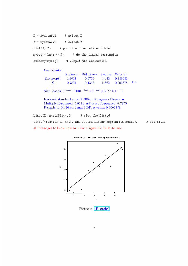
X = mydata$V1 # select X

Y = mydata$V2 # select Y

plot(X, Y) # plot the observations (data)

myreg = lm(Y ∼ X) # do the linear regression

summary(myreg) # output the estimation

Coefficients:Estimate Std. Error t value P r(> |t|)

(Intercept) 1.3931 0.9726 1.432 0.189932X 0.7874 0.1343 5.862 0.000378 ***—

Sign. codes: 0 ‘***’ 0.001 ‘**’ 0.01 ‘*’ 0.05 ‘.’ 0.1 ‘ ’ 1

Residual standard error: 1.406 on 8 degrees of freedomMultiple R-squared: 0.8111, Adjusted R-squared: 0.7875F-statistic: 34.36 on 1 and 8 DF, p-value: 0.0003778

lines(X, myreg$fitted) # plot the fitted

title("Scatter of (X,Y) and fitted linear regression model") # add title

# Please get to know how to make a figure file for latter use

2 4 6 8 10

2

4

6

8

1 0

X

Y

Scatter of (X,Y) and fitted linear regression model

Figure 1: (R code)

2

http://www.stat.nus.edu.sg/~staxyc/code010201.R

http://www.stat.nus.edu.sg/~staxyc/code010201.R



The fitted regression line/model is

ˆY = 1.3931 + 0.7874X

For any new subject/individual with X , its prediction of E (Y ) is

Y = b0 + b1X .

For the above data,

• If X = −3, then we predict Y = −0.9690

• If X

= 3, then we predict Y = 3.7553

• If X = 0.5, then we predict Y = 1.7868

2 Properties of Least squares estimators

Statistical properties in theory

• LSE is unbiased: E {b1} = β 1, E {b0} = β 0.

Proof: By the model, we have

Y = β 0 + β 1 X + ε

and

b1 =

ni=1(X i − X )(Y i − Y )n

i=1(X i − X )2

=

ni=1(X i − X )(β 0 + β 1X i + εi − β 0 − β 1 X − ε)n

i=1(X i − X )2

= β 1 + n

i=1(X i − ¯X )(εi − ε)n

i=1(X i − X )2

= β 1 +

ni=1(X i − X )εini=1(X i − X )2

recall that Eεi = 0. It follows that

Eb1 = β 1.

3



For b0,

E (b0

) = E (Y −

b1

X ) = β 0

+ β 1

X −

E (b1

) X = β 0

+ β 1

X −

β 1

X

= β 0

• Variance of the estimators

V ar(b1) = σ2ni=1(X i − X )2

, V ar(b0) = 1

nσ2 +

X 2ni=1(X i − X )2

σ2

[Proof:

V ar(b1) = V ar(

ni=1(X i − X )εi

n

i=1(X i − ¯X )

2 )

= {n

i=1

(X i − X )2}−2V ar{n

i=1

(X i − X )εi}

= {n

i=1

(X i − X )2}−2n

i=1

(X i − X )2σ2

= σ2ni=1(X i − X )2

.

We shall prove the second equation later.]

• Estimated (fitted) regression function Y i = b0 + b1X i. We also call Y i = b0 + b1X i thefitted value.

E {Y i} = EY i

[Proof:

E (Y i) = E (b0 + b1X i) = E (b0) + E (b1)X i = β 0 + β 1X i = EY i

]

Numerical properties of fitted regression line

Recall the normal equations

−2n

i=1

(Y i − b0 − b1X i) = 0

−2

ni=1

X i(Y i − b0 − b1X i) = 0

4



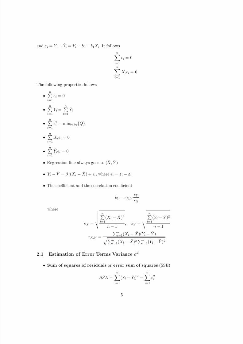
and ei = Y i − Y i = Y i − b0 − b1X i. It follows

n

i=1

ei = 0

ni=1

X iei = 0

The following properties follows

•n

i=1ei = 0

•n

i=1Y i =

ni=1

Y i

• ni=1

e2i = minb0,b1{Q}

•n

i=1X iei = 0

•n

i=1Y iei = 0

• Regression line always goes to ( X, Y )

• Y i − Y = β 1(X i − X ) + i, where i = εi − ε.

• The coefficient and the correlation coefficient

b1 = rX,Y sY sX

where

sX =

n

i=1(X i − X )2

n − 1 , sY =

n

i=1(Y i − Y )2

n − 1

rX,Y =

ni=1(X i − X )(Y i − Y )

ni=1(X i − X )2 ni=1(Y i − Y )2

2.1 Estimation of Error Terms Variance σ2

• Sum of squares of residuals or error sum of squares (SSE)

SSE =n

i=1

(Y i − Y i)2 =

ni=1

e2i

5



• Estimate σ2 by

s2

=

ni=1

(Y i − Y i)2

n − 2 =

ni=1

e2i

n − 2

called mean squared error (MSE), i.e.

M SE =

ni=1

e2i

n − 2

or denoted by σ2.

Why is it divided by n − 2? because there are TWO constraints on ei, i = 1,...,n, i.e.

the normal equations.

• s2 is unbiased estimator of σ2, i.e. E (s2) = σ2

[Proof: For any ξ 1,...,ξ n IID with mean µ and variance σ2, we have

E

ni=1

(ξ i − ξ )2 = E

ni=1

[(ξ i − µ)− (ξ − µ)]2

= E {n

i=1

(ξ i − µ)2 − n(ξ − µ)2}

=n

i=1

V ar(ξ )− nV ar(ξ )

= nσ2 − σ2

= (n − 1)σ2

This is why we estimate σ2 by

σ2 =

ni=1(ξ i − ξ )2

n − 1 .

Consider

V ar(ξ 1 − ξ ) = V ar{(1 − 1

n)ξ 1 −

n-1 terms 1

nξ 2 − ... − 1

nξ n}

= (1 − 1

n)2σ2 +

1

n2σ2 + ... +

1

n2σ2

= (1 − 2

n +

1

n2)σ2 +

n − 1

n2 σ2

= (1 − 1

n)σ2.

6



similarly, for any i,

V ar(ξ i − ¯ξ ) = (1 −

1

n )σ

2

.

Now turn to the estimator s2. Consider

E {n

i=1

(Y i − Y i)2} =

ni=1

E (Y i − Y i)2 =

ni=1

V ar(Y i − Y i) + {E (Y i − Y i)}2

=n

i=1

V ar{(Y i − Y − b1(X i − X ))2}

=n

i=1

{V ar(Y i − Y ) − 2Cov(Y i − Y , b1(X i − X )) + V ar(b1)(X i − X )2}

=n

i=1

{V ar(Y i − Y ) − 2Cov((Y i − Y )(X i − X ), b1) + V ar(b1)(X i − X )2}

=n

i=1

{V ar(εi − ε) − 2Cov((Y i − Y )(X i − X ), b1) + V ar(b1)(X i − X )2}

= (n − 1)σ2 − 2Cov(n

i=1

(Y i − Y )(X i − X ), b1) + V ar(b1)n

i=1

(X i − X )2

= (n − 1)σ2 − 2Cov(b1

ni=1

(X i − X )2, b1) + V ar(b1)n

i=1

(X i − X )2

= (n − 1)σ2 − V ar(b1)n

i=1

(X i − X )2 = (n − 2)σ2.

Thus

E (s2) = σ2

Example For the above example, the MSE (estimator of σ2 = V ar(εi)) is

M SE =n

i=1

e2i /(n − 2) = 1.975997.

or

σ =√

M SE = 1.405702

which is also called Residual standard error.

How to find the value in the output of R?

7



3 Regression Without Predictors

At first glance, it doesn’t seem that studying regression without predictors would be veryuseful. Certainly, we are not suggesting that using regression without predictors is a major

data analysis tool. We do think that it is worthwhile to look at regression models without

predictors to see what they can tell us about the nature of the constant. Understanding the

regression constant in these simpler models will help us to understand both the constant

and the other regression coefficients in later more complex models.

Model

Y i = β 0 + εi, i = 1, 2,...,n.

where as before, we assume

εi, i = 1, 2,...,n are IID with E (εi) = 0 and V ar(εi) = σ2

(We shall call this model Regression Without Predictors)

The least square estimator b0 is to minimizer of

Q =

ni=1

{Y i − b0}2

Note thatdQ

db0= −2

ni=1

{Y i − b0}

Letting it equal 0, we have the normal equation

ni=1

{Y i − b0} = 0

which leads to the (ordinary) least square estimator

b0 = Y .

The fitted model is

Y i = b0.

The fitted residuals are

ei = Y i − Y i = Y i − Y i

8



• Can you prove the estimator is unbiased, i.e E b0 = β 0?

• How to estimate σ2?

σ2 = 1

n − 1

ni=1

e2i

Why it is divided by n − 1?

4 Inference in regression

Next, we consider the simple linear regression model

Y 1 = β 0 + β 1X 1 + ε1

Y 2 = β 0 + β 1X 2 + ε2

... (1)

Y n = β 0 + β 1X n + εn

under assumptions of normal random errors.

• X i is a known, observed, and nonrandom

• ε1,...,εn are independent N (0, σ2

), Thus Y i is random

• β 0, β 1 and σ2 are parameters.

By the assumption, we have

E (Y i) = β 0 + β 1X i

and

V ar(Y i) = σ2

4.1 Inference of β 1

We need to check whether β 1 = 0 (or any other specified value, say -1.5), why

• To check whether X and Y has linear relationship

9



• To see whether the model can be simplified (if β 1 = 0, the model becomes Y i = β 0+εi,

a regression model without predictors.) For example, Hypotheses H 0 : β 1 = 0 v.s.

H a : β 1 = 0

Sample distribution of b1 recall

b1 =

ni=1(X i − X )(Y i − Y )n

i=1(X i − X )2

Theorem 4.1 For model (1) with normal assumption of εi then

b1 ∼ N

β 1, σ2ni=1(X i − X )2

Proof Recall the fact that any linear combination of independent normal distributed random

variables is still normal. To find its distribution, we only need to find its mean and variance .

Since Y i are normal and independent, thus b1 is normal, and

Eb1 = β 1

and (we have proved that)

V ar(b1) = σ2ni=1(X i − X )2

The theorem follows.

Question: what is the distribution of b1/ V ar(b1) under H 0? Can we use this Theorem

to test the hypothesis H 0? why

Estimated Variance of b1. (Estimating σ2 by M SE )

s2(b1) = MSE ni=1(X i − X )2

=

ni=1 e2i /(n − 2)ni=1(X i − X )2

s(b1) is the Standard Error (or S.E.) of b1, (or called Standard deviation)

sample distribution of (b1 − β 1)/s(b1)

b1 − β 1s(b1)

follows t(n − 2) for model (1)

Confidence interval for β 1. Let t1−α/2(n−2) or t(1−α/2, n−2) the 1−α/2−quantile

of t(n− 2).

P (t(α/2, n − 2) ≤ (b1 − β 1)/s(b1) ≤ t(1 − α/2, n − 2)) = 1 − α

10



By symmetry of the distribution, we have

t(1 − α/2, n − 2) = −t(α/2, n − 2)

Thus, with confidence 1 − α, we have the confidence interval for β 1 is

−t(1 − α/2, n − 2) ≤ (b1 − β 1)/s(b1) ≤ t(1 − α/2, n − 2)

i.e.

b1 − t(1 − α/2, n − 2) ∗ s(b1) ≤ β 1 ≤ b1 + t(1 − α/2, n − 2) ∗ s(b1)

Example 4.2 For the example above, find the 95% confidence interval for β 1?

solution: since n = 10, we have t(1− 0.05/2, 8) = 2.306; the SE for b1 is s(b1) = 0.1343.

Thus the confidence interval is

b1 ± t(1 − 0.05/2, 8) ∗ s(b1) = 0.7874 ± 2.306 ∗ 0.1343 = [0.4777, 1.0971]

Test of β 1

• Two-sided Test: to check whether β 1 is 0

H 0 : β 0 = 0, H a : β 1 = 0

Under H 0, we have random variable

t = b1s(b1)

∼ t(n − 2)

Suppose the significance level is α (usually, 0.05, 0.01). Calculate t, say t∗

– If |t∗| ≤ t(1 − α/2; n − 2), then accept H 0.

– If |t∗| > t(1 − α/2; n − 2), then reject H 0.

The test can also be done based on the p-value, defined as p = P (|t| > |t∗|). It is

easy to see that

p-value < α ⇐⇒ |t∗| > t(1 − α/2; n − 2)

Thus

11



– If p-value ≥ α, then accept H 0.

– If p-value < α, then reject H 0.

• One-sided test: for example to check whether β 1 is positive (or negative)

H 0 : β 1 ≥ 0, H a : β 1 < 0

Under H 0, we have

t = b1s(b1)

= b1 − β 1

s(b1) +

β 1s(b1)

∼ t(n − 2) + a positive term

Suppose the significance level is α (usually, 0.05, 0.01). Calculate t, say t∗

– If t∗ ≥ t(α; n − 2), then accept H 0.

– If t∗ < t(α; n − 2), then reject H 0.

4.2 Inference about β 0

Sample distribution of b0

b0 = Y − b1 X

Theorem 4.3 For model (1) with normal assumption of εi then

b0 ∼ N

β 0, σ2[1

n +

X 2ni=1(X i − X )2

]

[Proof The expectation is

Eb0 = E {Y } − E (b1) X = (β 0 + β 1 X ) − β 1 X = β 0

Let ki = (X i− X )n

i=1(X i− X )2

, then (see the proof at the beginning of this part)

b1 = β 1 +n

i=1

kiεi.

Thus

b0 = β 0 + 1

n

ni=1

εi −n

i=1

kiεi = β 0 +n

i=1

[1

n − ki X ]εi

The variance is

V ar(b0) =

ni=1

[1

n − ki X ]2σ2 = [

1

n +

X 2ni=1(X i − X )2

]σ2

12



Therefore the Theorem follows.]

Estimated Variance of b0 (by replacing σ2 with MSE).

s2(b0) = M SE 1

n +

X 2ni=1(X i − X )2

s(b0) is the Standard Error (or S.E.) of b0, (or called Standard deviation)

Sample distribution of (b0 − β 0)/s(b0)

b0 − β 0s(b0)

follows t(n − 2) for model (1)

Confidence interval for β 0: with confidence 1 − α, we have the confidence interval

b0 − t(1 − α/2, n − 2) ∗ s(b0) ≤ β 1 ≤ b0 + t(1 − α/2, n − 2) ∗ s(b0)

Test of β 0

• Two-sided Test: to check whether β 1 is 0

H 0 : β 0 = 0, H a : β 0

= 0

Under H 0, we have

t = b0s(b0)

∼ t(n − 2)

Suppose the significance level is α (usually, 0.05, 0.01). If the calculated t, say t∗

– If |t∗| ≤ t(1 − α/2; n − 2), then accept H 0.

– If |t∗| > t(1 − α/2; n − 2), then reject H 0.

Similarly, the test can also be done based on the p-value, defined as p = P (|t| > |t∗

|).It is easy to see that

p-value < α ⇐⇒ |t∗| > t(1 − α/2; n − 2)

Thus

– If p-value ≥ α, then accept H 0.

13



– If p-value < α, then reject H 0.

• One-sided test:to check whether β

1 is positive (or negative)

H 0 : β 0 ≤ 0, H a : β 0 > 0

Example 4.4 For the example above, with significance level 0.05,

1. Test H 0 : β 0 = 0 versus H 1 : β 0 = 0

2. Test H 0 : β 1 = 0 versus H 1 : β 1 = 0

3. Test H

0 : β 0 ≥ 0 versus H

1 : β 0 < 0

Answer:

1. since n = 10, t(0.975, 8) = 2.306. |t∗| = 1.432 < 2.306. Thus, we accept H 0

(another approach: p-value = 0.1899 > 0.05, we accept H 0)

2. The t-value is |t∗| = 5.862 > 2.306, thus we reject H 0, i.e. b1 is significantly different

from 0.

(another approach: p-value = 0.000378 < 0.05, we reject H 0)

3. t(0.05, 8) = −1.86, since t∗ = 1.3931 > −1.86 we accept H 0

How to find these test from the output of the R code?

14

math644_chapter 1_part2.pdf

Documents