MATH4427 Notebook 2 Fall Semester 2017/2018

prepared by Professor Jenny Baglivo

c© Copyright 2009-2018 by Jenny A. Baglivo. All Rights Reserved.

2 MATH4427 Notebook 2 3

2.1 Definitions and Examples . . . . . . . . . . . . . . . . . . . . . . . . . . . . . . . . . . . 3

2.2 Performance Measures for Estimators . . . . . . . . . . . . . . . . . . . . . . . . . . . . 5

2.2.1 Measuring Accuracy: Bias . . . . . . . . . . . . . . . . . . . . . . . . . . . . . . . 5

2.2.2 Measuring Precision: Mean Squared Error (MSE) . . . . . . . . . . . . . . . . . 7

2.2.3 Comparing Estimators: Efficiency . . . . . . . . . . . . . . . . . . . . . . . . . . 8

2.2.4 Another Performance Measure: Consistency . . . . . . . . . . . . . . . . . . . . . 9

2.3 Interval Estimation . . . . . . . . . . . . . . . . . . . . . . . . . . . . . . . . . . . . . . . 12

2.3.1 Error Probability, Confidence Coefficient, Confidence Interval . . . . . . . . . . . 12

2.3.2 Confidence Interval Procedures for Normal Distributions . . . . . . . . . . . . . . 14

2.4 Method of Moments (MOM) Estimation . . . . . . . . . . . . . . . . . . . . . . . . . . . 19

2.4.1 K th Moments and K th Sample Moments . . . . . . . . . . . . . . . . . . . . . . 19

2.4.2 MOM Estimation Method . . . . . . . . . . . . . . . . . . . . . . . . . . . . . . . 19

2.4.3 MOM Estimation Method for Multiple Parameters . . . . . . . . . . . . . . . . . 22

2.5 Maximum Likelihood (ML) Estimation . . . . . . . . . . . . . . . . . . . . . . . . . . . . 24

2.5.1 Likelihood and Log-Likelihood Functions . . . . . . . . . . . . . . . . . . . . . . 24

2.5.2 ML Estimation Method . . . . . . . . . . . . . . . . . . . . . . . . . . . . . . . . 24

2.5.3 Cramer-Rao Lower Bound . . . . . . . . . . . . . . . . . . . . . . . . . . . . . . . 29

2.5.4 Efficient Estimators; Minimum Variance Unbiased Estimators . . . . . . . . . . . 29

2.5.5 Large Sample Theory: Fisher’s Theorem . . . . . . . . . . . . . . . . . . . . . . . 32

2.5.6 Approximate Confidence Interval Procedures; Special Cases . . . . . . . . . . . . 33

2.5.7 Multinomial Experiments . . . . . . . . . . . . . . . . . . . . . . . . . . . . . . . 37

2.5.8 ML Estimation Method for Multiple Parameters . . . . . . . . . . . . . . . . . . 42

1

2

2 MATH4427 Notebook 2

There are two core areas of mathematical statistics: estimation theory and hypothesis testingtheory. This notebook is concerned with the first core area, estimation theory. The notesinclude material from Chapter 8 of the Rice textbook.

2.1 Definitions and Examples

1. Random Sample: A random sample of size n from the X distribution is a list,

X1, X2, . . ., Xn,

of n mutually independent random variables, each with the same distribution as X.

2. Statistic: A statistic is a function of a random sample (or random samples).

3. Sampling Distribution: The probability distribution of a statistic is known as its samplingdistribution. Sampling distributions are often difficult to find.

4. Point Estimator: A point estimator (or estimator) is a statistic used to estimate anunknown parameter of a probability distribution.

5. Estimate: An estimate is the value of an estimator for a given set of data.

6. Test Statistic: A test statistic is a statistic used to test an assertion.

Example: Normal distribution. Let X1, X2, . . ., Xn be a random sample from a normaldistribution with mean µ and standard deviation σ.

1. Sample Mean: The sample mean, X = 1n

∑ni=1Xi, is an estimator of µ. This statistic

has a normal distribution with mean µ and standard deviation σ/√n.

2. Sample Variance: The sample variance,

S2 =1

n− 1

n∑i=1

(Xi −X)2,

is an estimator of σ2. The distribution of this statistic is related to the chi-square.Specifically, the statistic V = (n−1)

σ2 S2 has a chi-square distribution with (n− 1) df.

If the numbers 90.8, 98.0, 113.0, 134.7, 80.5, 97.6, 117.6, 119.9 are observed, for example, then

1. x = 106.513 is an estimate of µ, and

2. s2 = 316.316 is an estimate of σ2

based on these observations.

3

X and S2 can also be used to test assertions about the parameters of a normal distribution.For example, X can be used to test the assertion that

“The mean of the distribution is 100.”

Example: Multinomial experiments. Consider a multinomial experiment with k out-comes whose probabilities are pi, for i = 1, 2, . . . , k.

The results of n independent trials of a multinomial experiment are usually presented to usin summary form: Let Xi be the number of occurrences of the ith outcome in n independenttrials of the experiment, for i = 1, 2, . . . , k. Then

1. Sample Proportions: The ith sample proportion,

pi =Xi

n,

(read “pi-hat”) is an estimator of pi, for i = 1, 2, . . . , k. The distribution of this statisticis related to the binomial distribution. Specifically, Xi = npi has a binomial distributionwith parameters n and pi.

2. Pearson’s statistic: Pearson’s statistic,

X2 =k∑i=1

(Xi − npi)2

npi,

can be used to test the assertion that the true probability list is (p1, p2, . . . , pk). The exactprobability distribution of X2 is hard to calculate. But, if n is large, the distribution ofPearson’s statistic is approximately chi-square with (k − 1) degrees of freedom.

Suppose that n = 40, k = 6 and (x1, x2, x3, x4, x5, x6) = (5, 7, 8, 5, 11, 4) is observed.

Thenp1 = 0.125, p2 = 0.175, p3 = 0.20, p4 = 0.125, p5 = 0.275, p6 = 0.10

are point estimates of the model proportions based on the observed list of counts. (It is commonpractice to use the same notation for estimators and estimates of proportions.)

If, in addition, we were interested in testing the assertion that all outcomes are equally likely,(that is, the assertion that pi = 1

6 for each i), then

x2obs =

6∑i=1

(xi − 40/6)2

40/6= 5.0

is the value of the test statistic for the observed list of counts.

4

2.2 Performance Measures for Estimators

Let X1, X2, . . . , Xn be a random sample from a distribution with parameter θ. The notation

θ = θ (X1, X2, . . . , Xn)

(read “theta-hat”) is used to denote an estimator of θ.

Estimators should be both accurate (measured using the center of the sampling distribution)and precise (measured using both the center and the spread of the sampling distribution).

2.2.1 Measuring Accuracy: Bias

1. Bias: The bias of the estimator θ is defined as follows:

BIAS(θ) = E(θ)− θ.

An accurate estimator will have little or no bias.

2. Unbiased/Biased Estimators: If E(θ) = θ, then θ is said to be an unbiased estimator ofthe parameter θ; otherwise, θ is said to be a biased estimator of θ.

3. Asymptotically Unbiased Estimator: If θ is a biased estimator satisfying

limn→∞

E(θ) = θ, where n is the sample size,

then θ is said to be an asymptotically unbiased estimator of θ.

Example: Normal distribution. Let X be the sample mean, S2 be the sample variance,and S be the sample standard deviation of a random sample of size n from a normal distributionwith mean µ and standard deviation σ.

Then

1. Sample Mean: X is an unbiased estimator of µ since E(X) = µ.

2. Sample Variance: S2 is an unbiased estimator of σ2 since E(S2) = σ2.

3. Sample Standard Deviation: S is a biased estimator of σ, with expectation

E(S) = σ

√2

n− 1

Γ(n/2)

Γ((n− 1)/2)6= σ.

Since E(S)→ σ as n→∞, S is an asymptotically unbiased estimator of σ.

5

Exercise. Another commonly used estimator of σ2 is

σ2 =1

n

n∑i=1

(Xi −X)2 =(n− 1)

nS2.

Demonstrate that σ2 is a biased estimator of σ2, but that it is asymptotically unbiased.

Exercise. Let X be the sample mean of a random sample of size n from a continuous uniformdistribution on the interval [0, b], and let b = 2X be an estimator of the upper endpoint b.

(a) Demonstrate that b is an unbiased estimator of b, and find the variance of the estimator.

(b) Use b to estimate b using the following observations: 3.64, 3.76, 2.53, 7.06, 5.71.

6

2.2.2 Measuring Precision: Mean Squared Error (MSE)

The mean squared error (MSE) of an estimator is the expected value of the square of thedifference between the estimator and the true parameter:

MSE(θ) = E((θ − θ)2).

A precise estimator will have a small mean squared error.

Mean Squared Error Theorem. Let X1, X2, . . . , Xn be a random sample froma distribution with parameter θ, and let θ be an estimator of θ. Then

1. MSE(θ) = V ar(θ) + (BIAS(θ))2.

2. If θ is an unbiased estimator of θ, then MSE(θ) = V ar(θ).

Exercise. Use the definitions of mean squared error and variance, and properties of expectation,to prove the theorem above.

7

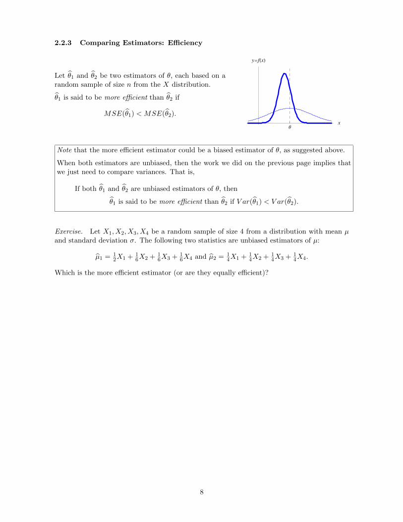
2.2.3 Comparing Estimators: Efficiency

Let θ1 and θ2 be two estimators of θ, each based on arandom sample of size n from the X distribution.

θ1 is said to be more efficient than θ2 if

MSE(θ1) < MSE(θ2).

θ�

�= �(�)

Note that the more efficient estimator could be a biased estimator of θ, as suggested above.

When both estimators are unbiased, then the work we did on the previous page implies thatwe just need to compare variances. That is,

If both θ1 and θ2 are unbiased estimators of θ, then

θ1 is said to be more efficient than θ2 if V ar(θ1) < V ar(θ2).

Exercise. Let X1, X2, X3, X4 be a random sample of size 4 from a distribution with mean µand standard deviation σ. The following two statistics are unbiased estimators of µ:

µ1 = 12X1 + 1

6X2 + 16X3 + 1

6X4 and µ2 = 14X1 + 1

4X2 + 14X3 + 1

4X4.

Which is the more efficient estimator (or are they equally efficient)?

8

A natural question to ask is whether a most efficient estimator exists. If we considerunbiased estimators only, we have the following definition.

MVUE: The unbiased estimator θ = θ(X1, X2, . . . , Xn) is said to be a minimumvariance unbiased estimator (MVUE) of θ if

V ar(θ) ≤ V ar(θ∗) for all unbiased estimators θ∗ = θ∗(X1, X2, . . . , Xn).

We will consider the question of finding an MVUE in Section 2.5.4 (page 29) of these notes.

2.2.4 Another Performance Measure: Consistency

The estimator θ = θ(X1, X2, . . . , Xn) is said to be a consistent estimator of θ if, for everypositive number ε,

limn→∞

P (|θ − θ| ≥ ε) = 0, where n is the sample size.

(A consistent estimator is unlikely to be far from the true parameter when n is large enough.)

Note that sample means are, in general, consistent estimators of distribution means. Thisfollows from the Law of Large Numbers from probability theory:

Law of Large Numbers. Let X be a random variable with mean µ = E(X) andstandard deviation σ = SD(X). Further, let

X = 1n

∑ni=1Xi

be the sample mean of a random sample of size n from the X distribution. Then,for every positive real number ε,

limn→∞

P (|X − µ| ≥ ε) = 0.

Importantly, consistent estimators are not necessarily unbiased, although they are often asymp-totically unbiased. If an estimator is unbiased, however, a quick check for consistency is givenin the following theorem.

Consistency Theorem. If θ is an unbiased estimator of θ satisfying

limn→∞

V ar(θ) = 0, where n is the sample size,

then θ is a consistent estimator of θ.

9

Exercise. One form of the Chebyshev inequality from probability theory says that

P (|Y − µy| ≥ kσy) ≤1

k2,

where Y is a random variable with mean µy = E(Y ) and standard deviation σy = SD(Y ), andk is a positive constant. Use this form of the Chebyshev inequality to prove the ConsistencyTheorem for unbiased estimators.

10

Exercise. Let X be the number of successes in n independent trials of a Bernoulli experimentwith success probability p, and let p = X

n be the sample proportion.

Demonstrate that p is a consistent estimator of p.

Exercise. Let S2 be the sample variance of a random sample of size n from a normal distributionwith mean µ and standard deviation σ.

Demonstrate that S2 is a consistent estimator of σ2.

11

2.3 Interval Estimation

Let X1, X2, . . . , Xn be a random sample from a distribution with parameter θ. The goal ininterval estimation is to find two statistics

L = L (X1, X2, . . . , Xn) and U = U (X1, X2, . . . , Xn)

with the property that θ lies in the interval [L,U ] with high probability.

2.3.1 Error Probability, Confidence Coefficient, Confidence Interval

1. Error Probability: It is customary to let α (called the error probability) equal the proba-bility that θ is not in the interval, and to find statistics L and U satisfying

(a) P (θ < L) = P (θ > U) = α2 and

(b) P (L ≤ θ ≤ U) = 1− α.

�-αα/� α/�� �

2. Confidence Coefficient: The probability (1− α) is called the confidence coefficient.

3. Confidence Interval: The interval [L,U ] is called a 100(1−α)% confidence interval for θ.

A 100(1−α)% confidence interval is a random quantity. In applications, we substitute samplevalues for the lower and upper endpoints and report the interval [`, u].

The reported interval is not guaranteed to contain the true parameter, but 100(1 − α)% ofreported intervals will contain the true parameter.

Example: Normal distribution with known σ. Let X be a normal random variable withmean µ and known standard deviation σ, and let X be the sample mean of a random sampleof size n from the X distribution.

The following steps can be used to find expressions for the lower limit L and the upper limitU of a 100(1− α)% confidence interval for the mean µ:

1. First note that Z = (X − µ)/√σ2/n is a standard normal random variable.

12

2. For convenience, let p = α/2. Further, let zp and z1−p be the pth and (1− p)th quantilesof the standard normal distribution. Then

P (zp ≤ Z ≤ z1−p) = 1− 2p.

3. The following statements are equivalent:

zp ≤ Z ≤ z1−p ⇐⇒ zp ≤ (X−µ)√σ2/n

≤ z1−p

⇐⇒ zp

√σ2

n ≤ (X − µ) ≤ z1−p

√σ2

n

⇐⇒ X − z1−p

√σ2

n ≤ µ ≤ X − zp√

σ2

n

Thus, P

(X − z1−p

√σ2

n ≤ µ ≤ X − zp√

σ2

n

)= 1− 2p.

4. Since zp = −z1−p and p = α/2, the expressions we want are

L = X − z1−α/2

√σ2

nand U = X − zα/2

√σ2

n= X + z1−α/2

√σ2

n.

Example. I used the computer to generate 50 random samples of size 16 from the normaldistribution with mean 0 and standard deviation 10. For each sample, I computed a 90%confidence interval for µ using the expressions for L and U from above.

The following plot shows the observed intervals as vertical line segments.

-��

-�

�

�

��

46 intervals contain µ = 0 (solid lines), while 4 do not (dashed lines).

[Question: If you were to repeat the computer experiment above many times, how manyintervals would you expect would contain 0? Why?]

13

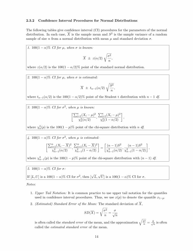
2.3.2 Confidence Interval Procedures for Normal Distributions

The following tables give confidence interval (CI) procedures for the parameters of the normaldistribution. In each case, X is the sample mean and S2 is the sample variance of a randomsample of size n from a normal distribution with mean µ and standard deviation σ.

1. 100(1− α)% CI for µ, when σ is known:

X ± z(α/2)

√σ2

n,

where z(α/2) is the 100(1− α/2)% point of the standard normal distribution.

2. 100(1− α)% CI for µ, when σ is estimated:

X ± tn−1(α/2)

√S2

n,

where tn−1(α/2) is the 100(1− α/2)% point of the Student t distribution with n− 1 df.

3. 100(1− α)% CI for σ2, when µ is known:[∑ni=1(Xi − µ)2

χ2n(α/2)

,

∑ni=1(Xi − µ)2

χ2n(1− α/2)

],

where χ2n(p) is the 100(1− p)% point of the chi-square distribution with n df.

4. 100(1− α)% CI for σ2, when µ is estimated:[∑ni=1(Xi −X)2

χ2n−1(α/2)

,

∑ni=1(Xi −X)2

χ2n−1(1− α/2)

]=

[(n− 1)S2

χ2n−1(α/2)

,(n− 1)S2

χ2n−1(1− α/2)

],

where χ2n−1(p) is the 100(1− p)% point of the chi-square distribution with (n− 1) df.

5. 100(1− α)% CI for σ:

If [L,U ] is a 100(1− α)% CI for σ2, then [√L,√U ] is a 100(1− α)% CI for σ.

Notes:

1. Upper Tail Notation: It is common practice to use upper tail notation for the quantilesused in confidence interval procedures. Thus, we use x(p) to denote the quantile x1−p.

2. (Estimated) Standard Error of the Mean: The standard deviation of X,

SD(X) =

√σ2

n=

σ√n

is often called the standard error of the mean, and the approximation√

S2

n = S√n

is often

called the estimated standard error of the mean.

14

Exercise. Demonstrate that the confidence interval procedure for estimating σ2 when µ isknown is correct.

15

Exercise. Assume that the following numbers are the values of a random sample from a normaldistribution with known standard deviation 10:

97.864 103.689 101.945 89.416 104.230 90.190 108.890 102.99385.746 104.759 89.685 117.986 83.084 96.150 96.324

Sample summaries: n = 15, x = 98.1967

Construct 80% and 90% confidence intervals for µ.

16

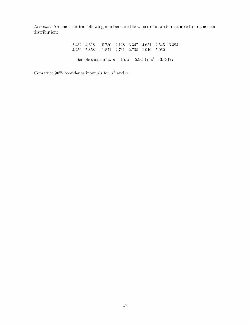
Exercise. Assume that the following numbers are the values of a random sample from a normaldistribution:

2.432 4.618 0.730 2.128 3.347 4.651 2.545 3.3933.250 5.858 −1.871 2.761 2.738 1.910 5.062

Sample summaries: n = 15, x = 2.90347, s2 = 3.53177

Construct 90% confidence intervals for σ2 and σ.

17

Exercise. As part of a study on body temperatures of healthy adult men and women, 30temperatures (in degrees Fahrenheit) were recorded:

98.2 98.2 98.4 98.4 98.6 98.7 98.7 98.7 98.8 98.898.8 98.9 99.0 99.1 99.9 97.1 97.4 97.4 97.6 97.697.8 97.8 98.0 98.2 98.6 98.6 98.8 99.0 99.1 99.4

Sample summaries: n = 30, x = 98.4533, s = 0.6463

Assume these data are the values of a random sample from a normal distribution.

Construct and interpret 95% confidence intervals for µ and σ.

18

2.4 Method of Moments (MOM) Estimation

The method of moments is a general method for estimating one or more unknown parameters,introduced by Karl Pearson in the 1880’s. In general, MOM estimators are consistent, butthey are not necessarily unbiased.

2.4.1 K th Moments and K th Sample Moments

1. The kth moment of the X distribution is

µk = E(Xk), for k = 1, 2, . . ., whenever the expected value converges.

2. The kth sample moment is the statistic

µk =1

n

n∑i=1

Xki , for k = 1, 2, . . .,

where X1, X2, . . ., Xn is a random sample of size n from the X distribution.

[Question: The kth sample moment is an unbiased and consistent estimator of µk, when µkexists. Can you see why?]

2.4.2 MOM Estimation Method

Let X1, X2, . . . , Xn be a random sample from a distribution with parameter θ, and supposethat µk = E(Xk) is a function of θ for some k.

Then, a method of moments estimator of θ is obtained using the following procedure:

Solve µk = µk for the parameter θ.

For example, let X1, X2, . . . , Xn be a random sample of size n from the continuous uniformdistribution on the interval [0, b]. Since E(X) = b/2, a method of moments estimator of theupper endpoint b can be obtained as follows:

µ1 = µ1 =⇒ E(X) = X =⇒ b

2= X =⇒ b = 2X .

Thus, b = 2X is a MOM estimator of b.

19

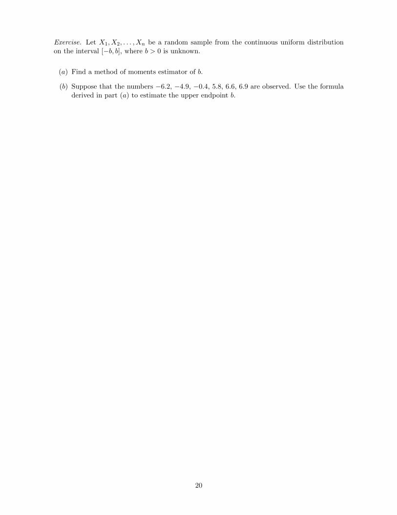
Exercise. Let X1, X2, . . . , Xn be a random sample from the continuous uniform distributionon the interval [−b, b], where b > 0 is unknown.

(a) Find a method of moments estimator of b.

(b) Suppose that the numbers −6.2, −4.9, −0.4, 5.8, 6.6, 6.9 are observed. Use the formuladerived in part (a) to estimate the upper endpoint b.

20

Exercise (slope-parameter model). Let X be a continuous random variable with range equal tothe interval (−1, 1) and with density function as follows:

f(x) =1

2(1 + αx) when x ∈ (−1, 1), and 0 otherwise,

where α ∈ (−1, 1) is an unknown parameter. Find a method of moments estimator of α basedon a random sample of size n from the X distribution.

21

2.4.3 MOM Estimation Method for Multiple Parameters

The method of moments procedure can be generalized to any number of unknown parameters.

For example, if the X distribution has two unknown parameters (say θ1 and θ2), then MOMestimators are obtained using the procedure:

Solve µk1 = µk1 and µk2 = µk2 simultaneously for θ1 and θ2.

Example: Normal distribution. Let X1, X2, . . . , Xn be a random sample from a nor-mal distribution with mean µ and variance σ2, where both parameters are unknown. Tofind method of moments estimators of µ and σ2, we need to solve two equations in the twounknowns.

Since E(X) = µ and E(X2) = V ar(X) + (E(X))2 = σ2 + µ2, we can use the equations

µ1 = µ1 and µ2 = µ2

to find the MOM estimators. Now (complete the derivation),

22

Example: Gamma distribution. Let X1, X2, . . . , Xn be a random sample from a gammadistribution with parameters α and β, where both parameters are unknown. To find methodof moments estimators of α and β we need to solve two equations in the two unknowns.

Since E(X) = αβ and E(X2) = V ar(X) + (E(X))2 = αβ2 + (αβ)2, we can use the equations

µ1 = µ1 and µ2 = µ2

to find the MOM estimators. Now (complete the derivation),

23

2.5 Maximum Likelihood (ML) Estimation

The method of maximum likelihood is a general method for estimating one or more unknownparameters. Maximum likelihood estimation was introduced by R.A. Fisher in the 1920’s. Ingeneral, ML estimators are consistent, but they are not necessarily unbiased.

2.5.1 Likelihood and Log-Likelihood Functions

Let X1, X2, . . . , Xn be a random sample from a distribution with a scalar parameter θ.

1. The likelihood function is the joint PDF of the random sample thought of as a functionof the parameter θ, with the random Xi’s left unevaluated:

Lik(θ) =

∏ni=1 p(Xi) when X is discrete∏ni=1 f(Xi) when X is continuous

2. The log-likelihood function is the natural logarithm of the likelihood function:

`(θ) = log(Lik(θ))

Note that it is common practice to use log() to denote the natural logarithm, and that thisconvention is used in the Mathematica system as well.

For example, if X is an exponential random variable with parameter λ, then

1. The PDF of X is f(x) = λe−λx when x > 0, and f(x) = 0 otherwise,

2. The likelihood function for the sample of size n is

Lik(λ) =n∏i=1

f(Xi) =n∏i=1

λe−λXi = λne−λ∑ni=1Xi , and

3. The log-likelihood function for the sample of size n is

`(λ) = log(λne−λ

∑ni=1Xi

)= n log(λ)− λ

n∑i=1

Xi.

2.5.2 ML Estimation Method

The maximum likelihood estimator (or ML estimator) of θ is the value that maximizes eitherthe likelihood function (Lik(θ)) or the log-likelihood function (`(θ)).

In general, ML estimators are obtained using methods from calculus.

24

Example: Bernoulli distribution. LetX1, X2, . . . , Xn be a random sample from a Bernoullidistribution with success probability p and let Y =

∑ni=1Xi be the sample sum. Then the ML

estimator of p is the sample proportion p = Y/n. To see this,

1. Since there are Y successes (each occurring with probability p) and n− Y failures (eachoccurring with probability 1− p), the likelihood and log-likelihood functions are

Lik(p) =n∏i=1

p(Xi) = pY (1− p)n−Y and `(p) = Y log(p) + (n− Y ) log(1− p).

2. The derivative of the log-likelihood function is `′(p) =Y

p− (n− Y )

(1− p).

3. There are three cases to consider:

Y = 0: If no successes are observed, then Lik(p) = (1− p)n is decreasing on [0, 1].The maximum value occurs at the left endpoint. Thus, p = 0.

Y = n: If no failures are observed, then Lik(p) = pn is increasing on [0, 1]. Themaximum value occurs at the right endpoint. Thus, p = 1.

0 < Y < n: In the usual case, some successes and some failures are observed. Workingwith the log-likelihood function we see that

`′(p) = 0 ⇒ Y

p=

(n− Y )

(1− p)⇒ Y (1− p) = p(n− Y ) ⇒ p =

Y

n.

Thus, p = Yn is the proposed ML estimator.

The second derivative test is generally used to check that the proposedestimator is a maximum. In this case, since

` ′′(p) = − Yp2− (n− Y )

(1− p)2and ` ′′(p) < 0,

the second derivative test implies that p = Yn is a maximum.

In all cases, the estimator is p = Yn .

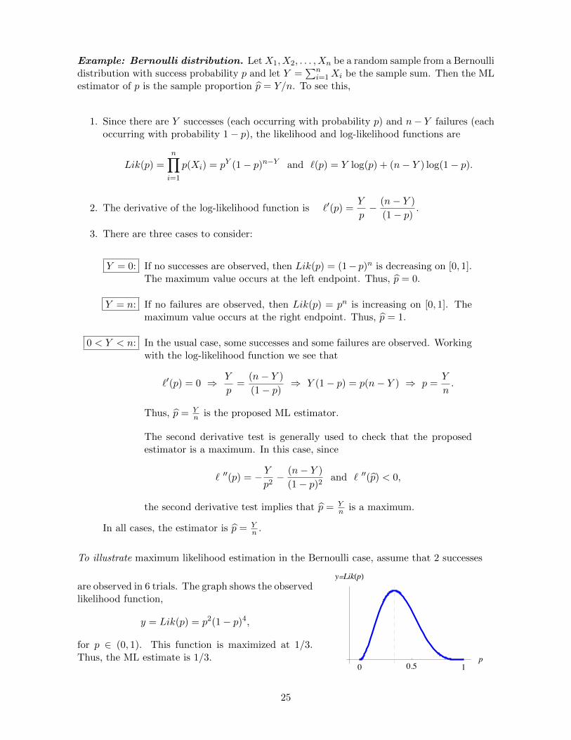
To illustrate maximum likelihood estimation in the Bernoulli case, assume that 2 successes

are observed in 6 trials. The graph shows the observedlikelihood function,

y = Lik(p) = p2(1− p)4,

for p ∈ (0, 1). This function is maximized at 1/3.Thus, the ML estimate is 1/3.

� ��� ��

�=���(�)

25

Example: Slope-parameter model. Let X be a continuous random variable with range(−1, 1) and with PDF as follows:

f(x) =1

2(1 + αx) when x ∈ (−1, 1) and 0 otherwise,

where α ∈ (−1, 1) is an unknown parameter.

Given a random sample of size n from the X distribution, the likelihood function is

Lik(α) =n∏i=1

f(Xi) =n∏i=1

(1 + αXi)

2=

1

2n

n∏i=1

(1 + αXi) ,

the log-likelihood simplifies to `(α) = −n log(2) +∑n

i=1 log(1 + αXi), and the first derivativeof the log-likelihood function is

`′(α) = .

Since the likelihood and log-likelihood functions are not easy to analyze by hand, we will usethe computer to find the ML estimate given specific numbers.

For example, assume that the following data are the values of a random sample from the Xdistribution:

0.455 −0.995 −0.101 0.568 0.298 −0.485 0.081 0.906−0.971 −0.337 0.278 0.714 0.175 0.414 −0.345 0.888

Sample summaries: n = 16, x = 0.0964375

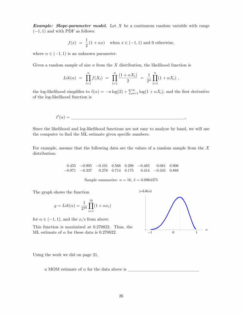
The graph shows the function

y = Lik(α) =1

216

16∏i=1

(1 + αxi)

for α ∈ (−1, 1), and the xi’s from above.

This function is maximized at 0.270822. Thus, theML estimate of α for these data is 0.270822. -� � �

α

�=���(α)

Using the work we did on page 21,

a MOM estimate of α for the data above is

26

Exercise: Poisson distribution. Let X1, X2, . . . , Xn be a random sample from a Poissondistribution with parameter λ, where λ > 0 is unknown. Let Y =

∑ni=1Xi be the sample sum,

and assume that Y > 0 .

Demonstrate that the ML estimator of λ is λ = Y/n.

27

Exercise: Uniform distribution on [0,b]. Let X1, X2, . . . , Xn be a random sample fromthe continuous uniform distribution on the interval [0, b], where b > 0 is unknown.

Demonstrate that b = max(X1, X2, . . . , Xn) is the ML estimator of b.

28

2.5.3 Cramer-Rao Lower Bound

The following theorem, proven by both Cramer and Rao in the 1940’s, gives a formula for thelower bound on the variance of an unbiased estimator of θ. The formula is valid under certain“smoothness conditions” on the X distribution.

Theorem (Cramer-Rao Lower Bound). Let X1, X2, . . . , Xn be a random sam-ple from a distribution with scalar parameter θ and let θ be an unbiased estimatorof θ. Under smoothness conditions on the X distribution:

V ar(θ) ≥ 1

nI(θ), where nI(θ) = −E(`′′(θ)).

In this formula, `′′(θ) is the second derivative of the log-likelihood function, andthe expectation is computed using the joint distribution of the Xi’s for fixed θ.

Notes:

1. Smoothness Conditions: If the following three conditions hold:

(a) The PDF of X has continuous second partial derivatives (except, possibly, at a finitenumber of points),

(b) The parameter θ is not at the boundary of possible parameter values, and

(c) The range of X does not depend on θ,

then X satisfies the “smoothness conditions” of the theorem.

The theorem excludes, for example, the Bernoulli distribution with p = 1 (condition 2 isviolated) and the uniform distribution on [0, b] (condition 3 is violated).

2. Fisher Information: The quantity nI(θ) is called the information in a sample of size n.

3. Cramer-Rao Lower Bound: The lower bound for the variance given in the theorem iscalled the Cramer-Rao lower bound; it is the reciprocal of the information, 1

nI(θ) .

2.5.4 Efficient Estimators; Minimum Variance Unbiased Estimators

Let X1, X2, . . . , Xn be a random sample from a distribution with parameter θ, and let θ be anestimator based on this sample. Then θ is said to be an efficient estimator of θ if

E(θ) = θ and V ar(θ) =1

nI(θ).

Note that if the X distribution satisfies the smoothness conditions listed above, and θ is anefficient estimator, then the Cramer-Rao theorem implies that θ is the minimum varianceunbiased estimator (MVUE) of θ.

29

Example: Bernoulli distribution. LetX1, X2, . . . , Xn be a random sample from a Bernoullidistribution with success probability p and let Y =

∑ni=1Xi be the sample sum.

Assume that 0 < Y < n . Then p = Yn is an efficient estimator of p.

To see this,

1. From the work we did starting on page 25, we know that p = Yn is the ML estimator of

the success probability p, and that the second derivative of the log-likelihood function is

`′′(p) = − Yp2− (n− Y )

(1− p)2.

2. The following computations demonstrate that the information nI(p) =n

p(1− p):

nI(p) = −E(` ′′(p))

= −E(− Yp2− (n− Y )

(1− p)2

)

=1

p2E(Y ) +

1

(1− p)2E(n− Y )

=1

p2(np) +

1

(1− p)2(n− np) since E(Y ) = nE(X) = np

=n

p+

n

(1− p)

=n(1− p) + np

p(1− p)=

n

p(1− p).

Thus, the Cramer-Rao lower bound is p(1−p)n .

3. The following computations demonstrate that p is an unbiased estimator of p with vari-ance equal to the Cramer-Rao lower bound:

E(p) = E

(Y

n

)=

1

nE(Y ) =

1

n(nE(X)) =

1

n(np) = p

V ar(p) = V ar

(Y

n

)=

1

n2V ar(Y ) =

1

n2(nV ar(X)) =

1

n2(np(1− p)) =

p(1− p)n

.

Thus, p is an efficient estimator of p.

30

Exercise: Poisson Distribution. Let X1, X2, . . . , Xn be a random sample from a Poissondistribution with parameter λ and let Y =

∑ni=1Xi be the sample sum. Assume that Y > 0 .

Demonstrate that λ = Y/n is an efficient estimator of λ.

31

2.5.5 Large Sample Theory: Fisher’s Theorem

R.A. Fisher proved a generalization of the Central Limit Theorem for ML estimators.

Fisher’s Theorem. Let θn be the ML estimator of θ based on a random sampleof size n from the X distribution, and

Zn =θn − θ√1/(nI(θ))

, where nI(θ) is the information.

Under smoothness conditions on the X distribution,

limn→∞

P (Zn ≤ x) = Φ(x) for every real number x,

where Φ(·) is the CDF of the standard normal random variable.

Notes:

1. Smoothness Conditions: The smoothness conditions in Fisher’s theorem are the sameones mentioned earlier.

2. Asymptotic Efficiency: If the X distribution satisfies the smoothness conditions and thesample size is large, then the sampling distribution of the ML estimator is approximatelynormal with mean θ and variance equal to the Cramer-Rao lower bound. Thus, the MLestimator is said to be asymptotically efficient.

It is instructive to give an outline of a key idea Fisher used to prove the theorem above.

1. Let `(θ) = log(Lik(θ)) be the log-likelihood function, and θ be the ML estimator.

2. Using the second order Taylor polynomial of `(θ) expanded around θ, we get

`(θ) ≈ `(θ) + `′(θ)(θ − θ) +`′′(θ)

2(θ − θ)2 = `(θ) +

`′′(θ)

2(θ − θ)2 since `′(θ) = 0.

3. Since Lik(θ) = e`(θ) = exp(`(θ)), we get

Lik(θ) ≈ exp

(`(θ) +

`′′(θ)

2(θ − θ)2

)= Lik(θ)e−(θ−θ)2/(2(−1/`′′(θ))).

The rightmost expression has the approximate form of the density function of a normaldistribution with mean θ and variance equal to the reciprocal of nI(θ) = −E(`′′(θ)).

32

2.5.6 Approximate Confidence Interval Procedures; Special Cases

Under the conditions of Fisher’s theorem, an approximate 100(1−α)% confidence interval forθ has the following form:

θ ± z(α/2)

√1

nI(θ)

where z(α/2) is the 100(1− α/2)% point of the standard normal distribution.

Exercise: Bernoulli Distribution. Let Y =∑n

i=1Xi be the sample sum of a randomsample of size n from a Bernoulli distribution with parameter p, where p ∈ (0, 1).

(a) Assume that the sample size n is large and that 0 < Y < n. Use Fisher’s theorem tofind the form of an approximate 100(1− α)% confidence interval for p.1

(b) Public health officials in Florida conducted a study to determine the level of resistanceto the antibiotic penicillin in individuals diagnosed with a strep infection. They chose asimple random sample of 1714 individuals from this population, and tested cultures takenfrom these individuals. In 973 cases, the culture showed partial or complete resistance tothe antibiotic. Use your answer to part (a) to construct an approximate 99% confidenceinterval for the proportion p of all individuals who would exhibit partial or completeresistance to penicillin when diagnosed with a strep infection. Interpret your interval.

1Note: The approximation is good when both E(Y ) = np > 10 and E(n− Y ) = n(1− p) > 10.

33

Exercise: Poisson Distribution. Let Y =∑n

i=1Xi be the sample sum of a random sampleof size n from a Poisson distribution with parameter λ, where λ > 0.

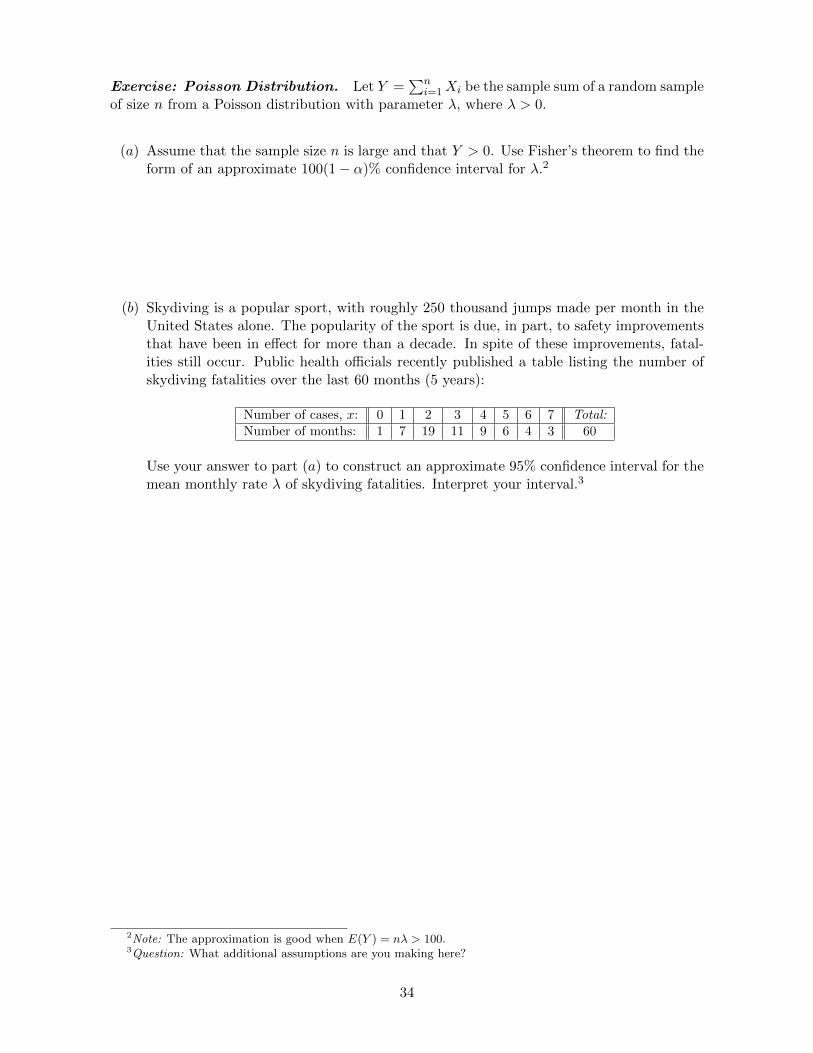
(a) Assume that the sample size n is large and that Y > 0. Use Fisher’s theorem to find theform of an approximate 100(1− α)% confidence interval for λ.2

(b) Skydiving is a popular sport, with roughly 250 thousand jumps made per month in theUnited States alone. The popularity of the sport is due, in part, to safety improvementsthat have been in effect for more than a decade. In spite of these improvements, fatal-ities still occur. Public health officials recently published a table listing the number ofskydiving fatalities over the last 60 months (5 years):

Number of cases, x: 0 1 2 3 4 5 6 7 Total:Number of months: 1 7 19 11 9 6 4 3 60

Use your answer to part (a) to construct an approximate 95% confidence interval for themean monthly rate λ of skydiving fatalities. Interpret your interval.3

2Note: The approximation is good when E(Y ) = nλ > 100.3Question: What additional assumptions are you making here?

34

Exercise: Exponential distribution. Let Y =∑n

i=1Xi be the sample sum of a randomsample of size n from an exponential distribution with parameter λ.

(a) Demonstrate that the ML estimator of λ is λ = n/Y .

(b) Demonstrate that nI(λ) = n/λ2.

35

(c) Assume that the sample size n is large. Use Fisher’s theorem to find the form of anapproximate 100(1− α)% confidence interval for λ.

(d) A university computer lab has 128 computers, which are used continuously from timeof installation until they break. The average time to failure for these 128 computerswas 1.523 years. Assume this information is a summary of a random sample from anexponential distribution. Use your answer to part (c) to construct an approximate 90%confidence interval for the exponential parameter λ. Interpret your interval.

36

2.5.7 Multinomial Experiments

Consider a multinomial experiment with k outcomes, each of whose probabilities is a functionof the scalar parameter θ:

pi = pi(θ), for i = 1, 2, . . . , k.

The results of n independent trials of a multinomial experiment are usually presented to usin summary form: Let Xi be the number of occurrences of the ith outcome in n independenttrials of the experiment, for i = 1, 2, . . . , k.

Since the random k-tuple (X1, X2, . . . , Xk) has a multinomial distribution, the likelihood func-tion is the joint PDF thought of as a function of θ with the Xi’s left unevaluated:

Lik(θ) =

(n

X1, X2, . . . , Xk

)p1(θ)X1 p2(θ)X2 · · · pk(θ)Xk .

We work with this likelihood when finding the ML estimator, the information, and so forth.

Exercise. Consider a multinomial experiment with 3 outcomes, whose probabilities are

p1 = p1(θ) = (1− θ)2, p2 = p2(θ) = 2θ(1− θ), p3 = p3(θ) = θ2,

where θ ∈ (0, 1) is unknown. Let Xi be the number of occurrences of the ith outcome in nindependent trials of the multinomial experiment, for i = 1, 2, 3. Assume each Xi > 0.

(a) Set up and simplify the likelihood and log-likelihood functions.

37

(b) Find the ML estimator, θ. Check that your estimator corresponds to a maximum.

38

(c) Find the information, nI(θ). In addition, report the Cramer-Rao lower bound.

(d) Find the form of an approximate 100(1− α)% confidence interval for θ.

39

Application: Hardy-Weinberg equilibrium model. In the Hardy-Weinberg equilibriummodel there are three outcomes, with probabilities:

p1 = (1− θ)2, p2 = 2θ(1− θ), p3 = θ2 .

The model is used in genetics. The usual setup is as follows:

1. Genetics is the science of inheritance. Hereditary characteristics are carried by genes,which occur in a linear order along chromosomes. A gene’s position along the chromosomeis also called its locus. Except for the sex chromosomes, there are two genes at everylocus (one inherited from mom and the other from dad).

2. An allele is an alternative form of a genetic locus.

3. Consider the simple case of a gene not located on one of the sex chromosomes, and withjust two alternative forms (i.e., two alleles), say A and a. This gives three genotypes:

AA, Aa, and aa.

4. Let θ equal the probability that a gene contains allele a. After many generations, theproportions of the three genotypes in a population are (approximately):

p1 = P (AA occurs) = (1− θ)2

p2 = P (Aa occurs) = 2θ(1− θ)p3 = P (aa occurs) = θ2

Exercise (Source: Rice textbook, Chapter 8). In a sample from the Chinese population in HongKong in 1937, blood types occurred with the following frequencies,

Blood type MM MN NNFrequency 342 500 187

where M and N are two types of antigens in the blood.

Assume these data summarize the values of a random sample from a Hardy-Weinberg equilib-rium model, where:

p1 = P (MM occurs) = (1− θ)2

p2 = P (MN occurs) = 2θ(1− θ)p3 = P (NN occurs) = θ2

40

Find the ML estimate of θ, the estimated proportions of each blood type (MM , MN , NN)in the population, and an approximate 90% confidence interval for θ.

41

2.5.8 ML Estimation Method for Multiple Parameters

If the X distribution has two or more unknown parameters, then ML estimators are computedusing the techniques of multivariable calculus.

Consider the two-parameter case under smoothness conditions, and let

`(θ1, θ2) = log(Lik(θ1, θ2)) be the log-likelihood function.

1. To find the ML estimators, we need to solve the following system of partial derivativesfor the unknown parameters θ1 and θ2:

`1(θ1, θ2) = 0 and `2(θ1, θ2) = 0,

where `i() is the partial derivative of the log-likelihood function with respect to θi.

2. To check that (θ1, θ2) is a maximum using the second derivative test, we need to checkthat the following two conditions hold:

d1 = `11(θ1, θ2) < 0 and d2 = `11(θ1, θ2)`22(θ1, θ2)− (`12(θ1, θ2))2 > 0,

where `ij() is the second partial derivative of the log-likelihood function, where youdifferentiate first with respect to θi and next with respect to θj .

Exercise: Normal distribution. Let X1, X2, . . ., Xn be a random sample of size n froma normal distribution with mean µ and variance σ2.

(a) Write L(µ, σ2) and `(µ, σ2). Simplify each function as much as possible.

42

(b) Find simplified forms for the first and second partial derivatives of `(µ, σ2).

43

(c) Demonstrate that the ML estimators of µ and σ2 are

µ = X and σ2 =1

n

n∑i=1

(Xi −X)2

and check that you have a maximum.

44

Example: Gamma distribution. Let X be a gamma random variable with shape parameterα and scale parameter β. Given a random sample of size n from the X distribution, thelikelihood and log-likelihood functions are as follows:

Lik(α, β) =∏ni=1

1Γ(α)βαX

α−1i e−Xi/β =

(1

Γ(α)βα

)n(ΠiXi)

α−1 e−ΣiXi/β

`(α, β) = −n log(Γ(α))− nα log(β) + (α− 1) log(ΠiXi)− ΣiXiβ

The partial derivatives of the log-likelihood with respect to α and β are as follows:

`1(α, β) =

`2(α, β) =

Since the system of equations `1(α, β) = 0 and `2(α, β) = 0 cannot be solved exactly, thecomputer is used to analyze specific samples.

For example, assume the following data are the values of a random sample from the X distri-bution:

8.68 8.91 11.42 12.04 12.47 14.6114.82 15.77 17.85 23.44 29.60 32.26

The graph below is a contour diagram of the observed log-likelihood function:

z = `(α, β) = −12 log(Γ(α))− 12α log(β) + (α− 1)(32.829)− 201.87

β.

• The contours shown in the graph correspond to

z = −39.6,−40.0,−40.4,−40.8.

• The function is maximized at (5.91, 2.85) (thepoint of intersection of the dashed lines).

• Thus, the ML estimate of (α, β) is (5.91, 2.85).� � � � ��

α

�

�

�

�

�

β

Note that, for these data, the MOM estimate of (α, β) is (5.17, 3.25).

45