Math3346 Assignment 1 – Solutions and Commentary

Lecturer: John Maindonald

March 14, 2014

General Comments

• Use tables to summarize information. Use text to draw attention to major features in thetables. Place the main focus on features that are clear and unequivocal, with more minormatters consigned to the later brief comment or to footnotes or endnotes.

• In an assignment such as this, most code should be included, properly referenced, at the end ofthe document. Including limited amounts of code in the text is acceptable, providing it has astrong “literate programming” character![In a report for a manager, omit code from the main document.]

• Round proportions to (in these data) 3 or 4 decimal places.

• Be judicious in the choice of graphs. If you have 10 or 12 graphs spread over 4 or 5 pages, youlikely need to find a more succinct form of presentation. Aim at a layout where it will be easyto identify the major differences. Overlaid plots of density estimates sometimes work well, foran audience that has some modest level of technical sophistication.

• Some forms of presentation that can be effective with an audience that has the right level oftechnically sophistication are not suited to use in reports that are intended for a general audience.Thus in considering use of, for example, density plots and boxplots, keep the audience in mind.

• Where a variable has missing values the total of zeros (or other such total) will be the totalof those known to be zero. On the (common) assumption that data are missing at random,division by the total of non-missing values gives an estimate of the proportion of zeros. If dataare not missing at random, then the number that results may be biased, perhaps so seriouslybiased that it is uninterpretable. This seems an issue for the variable re74 in the present data.

Solutions

1. Write brief notes on each of the columns of data, noting whether columns should be treated asnumeric or categorical. [1 mark]NB: Describe, where relevant, what codes 0 and 1 mean.Document (briefly) each of countNA(), countzeros() and countlist() [2 marks]

2. For each column of the data and for each of the four groups

(a) Determine the number of missing values. [1 mark]

age educ black hisp marr nodeg re74 re75 re78

cf-cps1 0 0 0 0 0 0 0 0 0

cf-psid1 0 0 0 0 0 0 0 0 0

exp -ctl 0 0 0 0 0 0 165 0 0

exp -trt 0 0 0 0 0 0 112 0 0

(b) For each of re74, re75 and re78, what number and proportion are zero. [1 mark]

cf-cps1 cf-psid1 exp -ctl exp -trt cf -cps1 cf -psid1 exp -ctl exp -trt

re74 1913 215 195 131 0.120 0.086 0.750 0.708

re75 1748 249 178 111 0.109 0.100 0.419 0.374

re78 2172 286 129 67 0.136 0.115 0.304 0.226

Note: The proportion of (known) zeros for re74 has been calculated relative to non-missingdata. This is the correct figure if missingness does not carry any information about income.For the present experimental data, this implies a massive change (> 30%, from ∼ 0.4 to >0.7) in the proportion of non-earners, between 1974 and 1975. As there is no comparablechange in the cps1 and psid1 data, this seems unlikely. Missing values for re74 seemthen unlikely to be missing at random. The variable re74 has therefore been ignored in thesubsequent discussion.

To calculate (known) zeros as a proportion of all data, change length(na.omit(x)) tolength(x). [Why would one want this?].

3. Now examine re74, comparing control and treatment data:

(a) Compare the proportion of NAs between the experimental control and treatment. [ 12 mark]

0 1

0.388 0.377

(b) Compare the proportion of 0’s in each of re74, re75 and re78 (obviously NAs have to beexcluded) between the four groups. [ 12 mark]

cf-cps1 cf-psid1 exp -ctl exp -trt

re74 0.120 0.086 0.750 0.708

re75 0.109 0.100 0.419 0.374

re78 0.136 0.115 0.304 0.226

(c) For columns that are numeric with more than two unique values, determine for each of thefour groups the range of values. [1 mark]

age -l age -u educ -l educ -u re74 -l re74 -u re75 -l re75 -u re78 -l

cf-cps1 16 55 0 18 0 25862 0 25244 0

cf-psid1 18 55 0 17 0 137149 0 156653 0

exp -ctl 17 55 3 14 0 39571 0 36941 0

exp -trt 17 49 4 16 0 35040 0 37432 0

re78 -u

cf-cps1 25565

cf-psid1 121174

exp -ctl 39484

exp -trt 60308

4. Provide graphs that conveniently summarise differences between the four groups, with respectto age and re75. [4 marks]

Age Education (yrs) Income in 1975

Den

sity

0.00

0.02

0.04

0.06

10 20 30 40 50 60

age

0.0

0.2

0.4

0.6

10 20 30 40

educ

0.0

0.2

0.4

0.6

0.8

−36111 21989

log(re75 + 37)

cf−cps1 cf−psid1 exp−ctl exp−trt

Figure 1: Densityplot comparisons, for Age, for Years of education and for log(re75+37). Thelogarithmic transformation leads to a more symmetric distribution. The plot for log(re75+37 has aspike at zero that, in the density plot, is spread either side of zero.

2

Age Education (yrs) Income in 1975

cf−cps1

cf−psid1

exp−ctl

exp−trt

20 30 40 50

age

10 20 30 40

educ

−36 111 21989

log(re75 + 37)

Figure 2: Boxplot comparisons, for Age, for Years of education, and for log(re75+37). The logarith-mic transformation leads to a more symmetric distribution. The plot for log(re75+37 has a spike atzero.

Density plots do not work well with educ. Hence we try histograms.

educ

Per

cent

of T

otal

0

10

20

30

40

0 5 10 15

cf−cps1

0 5 10 15

cf−psid1

0 5 10 15

exp−ctl

0 5 10 15

exp−trt

Figure 3: Histograms, used to compare distributions of Years of education.

• With one density plot for all data area under the curve gives an indication the density ofpoints, but the reader has to know or warned of the spike at zero, and to work on interpretingthe graph. Alternatively, zeros can be omitted, with information provided on the proportionof zeros. Histograms are also acceptable (with a relatively large number of data points, theirdiscreteness is not too much of an issue). They do not however readily lend themselves tooverlaying.

• A logarithmic scale seems preferable for re75; otherwise the graph focuses unduly on asmall number of very large values.

• Half the minimum non-zero value may be a reasonable offset when taking logarithms. Al-ternatively, choose the offset that leads to a near symmetric density plot.

The assignment did not ask for a graph for years of education, but it (or something like it) isneeded for the comparison in Exercise 6.

5. Use tables to summarise differences in categorical variables between the two groups. [2 marks]

3

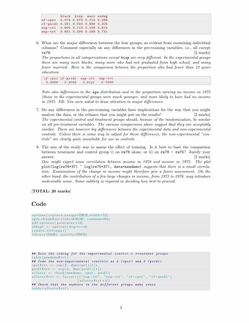
black hisp marr nodeg

cf-cps1 0.074 0.072 0.712 0.296

cf-psid1 0.251 0.033 0.866 0.305

exp -ctl 0.800 0.113 0.158 0.814

exp -trt 0.801 0.094 0.168 0.731

6. What are the major differences between the four groups, as evident from examining individualcolumns? Comment especially on any differences in the pre-training variables, i.e., all exceptre78. [3 marks]The proportions in all categorizations except hisp are very different. In the experimental groupsthere are many more blacks, many more who had not graduated from high school, and manyfewer married. Here is the comparison between the proportion who had fewer than 12 yearseducation:

cf -cps1 cf -psid1 exp -ctl exp -trt

0.2958 0.3052 0.8141 0.7306

Note also differences in the age distribution and in the proportion earning no income in 1975(those in the experimental groups were much younger, and more likely to have had no incomein 1975. NB: You were asked to draw attention to major differences.

7. Do any differences in the pre-training variables have implications for the way that you mightanalyse the data, or the reliance that you might put on the results? [2 marks]The experimental control and treatment groups should, because of the randomization, be similaron all pre-treatment variables. The various comparisons above suggest that they are acceptablysimilar. There are however big differences between the experimental data and non-experimentalcontrols. Unless there is some way to adjust for these differences, the non-experimental ”con-trols” are clearly quite unsuitable for use as controls.

8. The aim of the study was to assess the effect of training. Is it best to base the comparisonbetween treatment and control group i) on re78 alone, or ii) on re78 - re75? Justify youranswer. [2 marks]One might expect some correlation between income in 1978 and income in 1975. The plotplot(log(re78+37) ~ log(re75+37), data=nswdemo) suggests that there is a small correla-tion. Examination of the change in income might therefore give a fairer assessment. On theother hand, the contribution of a few large changes in income, from 1975 to 1978, may introduceundesirable noise. Some subtlety is required in deciding how best to proceed.

[TOTAL: 20 marks]

Code

opt ions ( r e p l a c e . a s s i g n=TRUE, width=72)opts chunk $ s e t ( t idy=FALSE, comment=NA)pd f . op t i on s ( p o i n t s i z e =12)o ldopt ← opt ions ( d i g i t s =4)r e n d e r l i s t i n g s ( )l i b r a r y (DAAG, qu i e t l y=TRUE)

## Note the coding for the experimental control & treatment groups

t ab l e (nswdemo$ t r t )## Code the non-experimental controls as 2 (cps1) and 3 (psid1)

cps1 $ t r t ← rep (2 , dim( cps1 ) [ 1 ] )ps id1 $ t r t ← rep (3 , dim( ps id1 ) [ 1 ] )a l l s e t s ← rbind (nswdemo , cps1 , ps id1 )a l l s e t s $ t r t ← f a c t o r ( c ( ” exp−ctl ” , ” exp−trt ” , ” cf−cps1 ” , ” cf−psid1 ” )

[ a l l s e t s $ t r t +1])## Check that the numbers in the different groups make sense

t ab l e ( a l l s e t s $ t r t )

4

## Function that retrieves number of NAs for a single column

countNA ← f unc t i on (x )sum( i s . n a (x ) )## Now use the function aggregate () to apply countNA () to

## allsets , indexed by trt

aggregate ( a l l s e t s , l i s t ( group = a l l s e t s $ t r t ) , FUN = countNA)

countze ros ← f unc t i on (x )sum( ! i s . n a (x ) & x==0)aggregate (nswdemo [ , c ( ” re74 ” , ” re75 ” , ” re78 ” ) ] , by=l i s t ( group=nswdemo$ t r t ) ,

FUN=countzeros )aggregate ( a l l s e t s [ , c ( ” re74 ” , ” re75 ” , ” re78 ” ) ] , l i s t ( group=a l l s e t s $ t r t ) ,

FUN=countzeros )

Alternative

## Function that retrieves number of NAs for each column of a data frame

c o u n t l i s t ← f unc t i on ( z , s t a t s f un=length ) sapply ( z , s t a t s f un )# Notice that statsfun has been given a default argument

## Apply this to the allsets data frame

sapply ( s p l i t ( a l l s e t s , a l l s e t s $ t r t ) , FUN=coun t l i s t , s t a t s f un=countNA)

Alternative data object

l i s t s e t s ← l i s t ( ” cf−cps1 ”=cps1 [ ,−1 ] , ” cf−psid1 ”=ps id1 [ ,−1 ] ,” exp−ctl ”=subset (nswdemo , t r t ==0)[ ,−1 ] ,” exp−trt ”=subset (nswdemo , t r t ==1)[ ,−1 ] )

## Check that the numbers in the different groups make sense

sapply ( l i s t s e t s , nrow )## Now do the calculations with listsets

sapply ( l i s t s e t s , FUN=coun t l i s t , s t a t s f un=countNA)

Code for exercises

1. . . .

2.

(a) t ( sapply ( l i s t s e t s , FUN=coun t l i s t , s t a t s f un=countNA ) )

(b) num ← sapply ( s p l i t ( a l l s e t s [ , c ( ” re74 ” , ” re75 ” , ” re78 ” ) ] ,a l l s e t s $ t r t ) , FUN=coun t l i s t , s t a t s f un=countze ros )

pr ← sapply ( s p l i t ( a l l s e t s [ , c ( ” re74 ” , ” re75 ” , ” re78 ” ) ] ,a l l s e t s $ t r t ) , FUN=coun t l i s t ,

s t a t s f un=func t i on (x ) countze ros ( x ) / l ength ( na.omit ( x ) ) )cbind (num, round ( pr , 3 ) )

Note: The above uses a “put as much as possible onto one line” style of code that iscompact and easy to manage, but which novices may find overly cryptic. The less condensedcode that now follows is more explicit. It works with smaller units of data, which is aconsideration if datasets are large relative to available memory. There is some redundancy,which should be removed if these calculations are repeated a large number of times. Themore obvious ways to remove the redundancy lead to code that is, again, somewhat morecryptic.

## Longer , less cryptic and clearer code , for exptl data only

namre ← c ( ” re74 ” , ” re75 ” , ” re78 ” )expc t l z ← sapply ( subset (nswdemo [ , namre ] , nswdemo$ t r t ==0), countzeros )expt r t z ← sapply ( subset (nswdemo [ , namre ] , nswdemo$ t r t ==1), countzeros )numz ← cbind ( expc t l=expct l z , expt r t=expt r t z )expct lp ← sapply ( subset (nswdemo [ , namre ] , nswdemo$ t r t ==0),

f unc t i on (x ) countze ros ( x ) / l ength ( na.omit ( x ) ) )exptrtp ← sapply ( subset (nswdemo [ , namre ] , nswdemo$ t r t ==1),

f unc t i on (x ) countze ros ( x ) / l ength ( na.omit ( x ) ) )propz ← cbind ( ” expctl−p”=expct lp , ” exptrt−p”=exptrtp )cbind (numz , propz )

expctl exptrt expctl -p exptrt -p

re74 195 131 0.7500 0.7081

re75 178 111 0.4188 0.3737

re78 129 67 0.3035 0.2256

5

3.

(a) round ( with (nswdemo , sapply ( s p l i t ( re74 , t r t ) ,f unc t i on (x ) countNA(x ) / l ength (x ) ) ) , 3)

(b) round ( sapply ( s p l i t ( a l l s e t s [ , c ( ” re74 ” , ” re75 ” , ” re78 ” ) ] ,a l l s e t s $ t r t ) , FUN=coun t l i s t ,

s t a t s f un=func t i on (x ) countze ros ( x ) / l ength ( na.omit ( x ) ) ) , 3)

(c) varnam ← c ( ”age” , ”educ” , ” re74 ” , ” re75 ” , ” re78 ” )ran ← sapply ( s p l i t ( a l l s e t s [ , varnam ] ,

a l l s e t s $ t r t ) , FUN=coun t l i s t ,s t a t s f un=func t i on (x ) range (x , na.rm=TRUE) )

rownames ( ran ) ← paste ( rep (varnam , rep (2 , l ength ( varnam ) ) ) , ”−” ,rep ( c ( ” l ” , ”u” ) , l ength ( varnam ) ) , sep=”” )

p r i n t ( round ( t ( ran ) , 0 ) )

l i b r a r y ( l a t t i c e )at1 ← pre t ty ( a l l s e t s $age , 5 )l abs1 ← paste ( at1 )at2 ← pre t ty ( a l l s e t s $educ , 5 )l abs2 ← paste ( at1 )at3 ← with ( a l l s e t s , p re t ty ( l og ( re75 +37) , 3 ) )at3 ← c ( l og (37 ) , at2 [ at2>l og ( 7 5 ) ] )l abs3 ← paste ( round ( exp ( at2 ) − 37 , 0 ) )p r i n t ( d en s i t yp l o t (∼age+educ+log ( re75 +37) , groups=tr t , auto .key=l i s t ( columns=4) ,

s c a l e s=l i s t ( x=l i s t ( at=l i s t ( at1 , at2 , at3 ) ,l a b e l s=l i s t ( labs1 , labs2 , l abs3 ) ) , r e l a t i o n=” f r e e ” ) ,

xlab=c ( ”Age” , ”Education ( yrs ) ” , ”Income in 1975” ) ,data=a l l s e t s ) )

p r i n t ( bwplot ( t r t∼age+educ+log ( re75 +37) , outer=TRUE,s c a l e s=l i s t ( x=l i s t ( at=l i s t ( at1 , at2 , at3 ) ,

l a b e l s=l i s t ( labs1 , labs2 , l abs3 ) , r e l a t i o n=” f r e e ” ) ) ,x lab=c ( ”Age” , ”Education ( yrs ) ” , ”Income in 1975” ) ,data=a l l s e t s ) )

p r i n t ( histogram (∼educ | t r t , data=a l l s e t s , l ayout=c ( 4 , 1 ) ) )

4.5. cat2prop ← f unc t i on (x ) i f ( i s . f a c t o r ( x ) ) sum(x==l e v e l s ( x ) [ 2 ] ) / l ength (x ) e l s esum(x==max(x ) ) / l ength (x )

contnum ← match ( c ( ” t r t ” , varnam ) , names ( a l l s e t s ) )t ( round ( sapply ( s p l i t ( a l l s e t s [ , −contnum ] ,

a l l s e t s $ t r t ) , FUN=coun t l i s t , s t a t s f un=cat2prop ) , 3 ) )

## Proportion with less than 12 years education

with ( a l l s e t s , sapply ( s p l i t ( educ , t r t ) , f unc t i on (x )sum(x<12) / l ength (x ) ) )

Use of the doBy Package

The summaryBy() function (doBy Package) has extensive abilities for calculating summary informa-tion. It returns a data frame. The following does the calculation required to calculate, for each of thenominated splits of the data and for each of the nominated columns, the number of zeros:

l i b r a r y (doBy)

Loading required package: survival

Loading required package: splines

Attaching package: ’survival ’

The following object is masked from ’package:DAAG ’:

lung

6

Loading required package: MASS

Attaching package: ’MASS ’

The following object is masked from ’package:DAAG ’:

hills

## The "0s" gets added to the names of the variables

countze ros ← f unc t i on (x ) c ( ”0 s ”=sum( ! i s . n a (x ) & x==0))num0 ← summaryBy( re74 + re75 + re78 ∼ t r t , data=a l l s e t s , FUN=countzeros )

The first column is a factor, with one row for each level of trt. The level names are better usedto label the rows. The first column can then be omitted, leaving a data frame that has all columnsnumeric.

row.names (num0) ← a s . c h a r a c t e r (num0 [ , 1 ] )

Then print(num0[, -1]) prints with the levels of trt used as row names, while print(t(num0[,

-1])) prints without the quotes that would otherwise appear.[The object t(num0) is a matrix of character. It has to be character because its first row is character.The command print(t(num0), quote=FALSEALSE)) can be used to print it without the quotes.]

7