Math 2200 – Discrete MathematicsSummer 2015

Instructor: Davar Khoshnevisan (davar@math.utah.edu)Department of Mathematics, University of Utah

Text: Discrete Mathematics by K.H. Rosen,McGraw Hill, NY, Seventh Edition, 2011

Contents

1 Introduction 31.1 Some Questions . . . . . . . . . . . . . . . . . . . . . . . . . . . . . 31.2 Topics Covered . . . . . . . . . . . . . . . . . . . . . . . . . . . . . 4

2 Elementary Logic 52.1 Propositional Logic . . . . . . . . . . . . . . . . . . . . . . . . . . . 52.2 Equivalences and Tautologies . . . . . . . . . . . . . . . . . . . . . 72.3 Predicates and Quantifiers . . . . . . . . . . . . . . . . . . . . . . 9

3 Logic in Mathematics 133.1 Some Terminology . . . . . . . . . . . . . . . . . . . . . . . . . . . 133.2 Proofs . . . . . . . . . . . . . . . . . . . . . . . . . . . . . . . . . . . 14

3.2.1 Proof by Exhaustion . . . . . . . . . . . . . . . . . . . . . . 143.2.2 Proof by Contradiction . . . . . . . . . . . . . . . . . . . . 143.2.3 Proof by Induction . . . . . . . . . . . . . . . . . . . . . . . 15

4 Naive Set Theory 204.1 Some Terminology . . . . . . . . . . . . . . . . . . . . . . . . . . . 204.2 The Calculus of Set Theory . . . . . . . . . . . . . . . . . . . . . . 224.3 Set Identities . . . . . . . . . . . . . . . . . . . . . . . . . . . . . . . 27

5 Transformations 295.1 Functions . . . . . . . . . . . . . . . . . . . . . . . . . . . . . . . . . 295.2 The Graph of a Function . . . . . . . . . . . . . . . . . . . . . . . 315.3 One-to-One Functions . . . . . . . . . . . . . . . . . . . . . . . . . 345.4 Onto Functions . . . . . . . . . . . . . . . . . . . . . . . . . . . . . 355.5 Inverse Functions . . . . . . . . . . . . . . . . . . . . . . . . . . . . 365.6 Composition of Functions . . . . . . . . . . . . . . . . . . . . . . . 375.7 Back to Set Theory: Cardinality . . . . . . . . . . . . . . . . . . . 38

6 Patterns and Sequences 446.1 Recurrence Relations . . . . . . . . . . . . . . . . . . . . . . . . . 446.2 Infinite Series . . . . . . . . . . . . . . . . . . . . . . . . . . . . . . 466.3 Continued Fractions . . . . . . . . . . . . . . . . . . . . . . . . . . 48

7 Elements of Number Theory 527.1 Division . . . . . . . . . . . . . . . . . . . . . . . . . . . . . . . . . . 527.2 Modular Arithmetic . . . . . . . . . . . . . . . . . . . . . . . . . . . 547.3 Representation of Integers . . . . . . . . . . . . . . . . . . . . . . 557.4 Examples of Binary Arithmetic . . . . . . . . . . . . . . . . . . . 57

1

7.5 Prime Numbers . . . . . . . . . . . . . . . . . . . . . . . . . . . . . 597.6 Divisibility Rules . . . . . . . . . . . . . . . . . . . . . . . . . . . . . 627.7 GCDs, LCMs, and the Euclidean Algorithm . . . . . . . . . . . . 64

8 Elements of Cryptography 688.1 Symmetric Ciphers . . . . . . . . . . . . . . . . . . . . . . . . . . . 688.2 Fancier Symmetric Coding Methods . . . . . . . . . . . . . . . . 708.3 Asymmetric Cryptography . . . . . . . . . . . . . . . . . . . . . . 71

9 Modular Inversion & Some of Its Applications 729.1 Bezout’s Theorem . . . . . . . . . . . . . . . . . . . . . . . . . . . . 729.2 Modular Inversion . . . . . . . . . . . . . . . . . . . . . . . . . . . 749.3 The Chinese Remainder Theorem . . . . . . . . . . . . . . . . . 769.4 Fermat’s Little Theorem . . . . . . . . . . . . . . . . . . . . . . . . 799.5 An Application to Asymmetric Encryption (RSA) . . . . . . . . . 81

10 Elements of Combinatorics 8310.1 Enumeration . . . . . . . . . . . . . . . . . . . . . . . . . . . . . . . 8310.2 Partitions . . . . . . . . . . . . . . . . . . . . . . . . . . . . . . . . . 8910.3 Examples from Poker . . . . . . . . . . . . . . . . . . . . . . . . . 9210.4 The Multinomial Summation Formula . . . . . . . . . . . . . . . 9410.5 The Pigeonhole Principle . . . . . . . . . . . . . . . . . . . . . . . 95

2

Module 1Introduction

There is a story about two friends, who were classmates in highschool, talking about their jobs. One of them became a statistician andwas working on population trends. He showed a reprint to his formerclassmate. The reprint started, as usual, with the Gaussian distributionand the statistician explained to his former classmate the meaning of thesymbols for the actual population, for the average population, and so on.His classmate was a bit incredulous and was not quite sure whetherthe statistician was pulling his leg. “How can you know that?” washis query. “And what is this symbol here?” “Oh,” said the statistician,“this is π.” “What is that?” “The ratio of the circumference of thecircle to its diameter.” “Well, now you are pushing your joke too far,“said the classmate, “surely the population has nothing to do with thecircumference of the circle.”

......

......

The preceding two stories illustrate the two main points which arethe subjects of the present discourse. The first point is that mathemat-ical concepts turn up in entirely unexpected connections. Moreover,they often permit an unexpectedly close and accurate description ofthe phenomena in these connections. Secondly, just because of thiscircumstance, and because we do not understand the reasons of theirusefulness, we cannot know whether a theory formulated in terms ofmathematical concepts in uniquely appropriate. We are in a positionsimilar to that of a man who was provided with a bunch of keys andwho, having to open several doors in succession, always hit on the rightkey on the first or second trial.

–Eugene Paul Wagner1

1.1. Some Questions

- Is mathematics a natural science, or is it a human invention?

- Is mathematics the science of laboriously doing the same things overand over, albeit very carefully? If yes, then why is it that some peoplediscover truly-novel mathematical ideas whereas many others do not?Or, for that matter, why can’t we seem to write an algorithm that doesnew mathematics for us? If no, then is mathematics an art?

1“The unreasonable effectiveness of mathematics in the natural sciences,” Communicationsin Pure and Applied Mathematics (1960) vol. 13, no. 1.

3

- Is mathematics a toolset for doing science? If so, then why is it thatthe same set of mathematical ideas arise in so many truly-differentscientific disciplines? Is mathematics a consequence of the humancondition, or is it intrinsic in the physical universe?

- Why is it that many people are perfectly comfortable saying some-thing like, “I can’t do mathematics,” or “I can’t draw,” but very few arecomfortable saying, “I can’t read,” or “I can’t put on my socks in themorning”?

- Our goal, in this course, is to set forth elementary aspects of the lan-guage of mathematics. The language can be learned by most people,though perhaps with effort. Just as most people can learn to read orput on their socks in the morning. [What one does with this elaboratelanguage then has to do with one’s creativity, intellectual curiosity, andother less tangible things.]

1.2. Topics Covered

- Propositional Logic, Modus Ponens, and Set Theory [Chapters 1-2, 5]

- Patterns [Chapter 3 and lecture notes]

- Number Theory and Cryptography [Chapter 4]

- Enumerative Combinatorics [Chapter 6 and a little of Chapter 7]

4

Module 2Elementary Logic

2.1. Propositional Logic

According to the Merriam-Webster online dictionary, “Logic” could meanany one of the following:

- A proper or reasonable way of thinking about or understanding some-thing;

- A particular way of thinking about something; and/or

- The science that studies the formal processes used in thinking andreasoning.

“Propositional logic” and its natural offspring, predicate logic, are early at-tempts to make explicit this process. Propositional logic was developed inthe mid-19th century by Augustus DeMorgan, George Boole, and others,and is sometimes also referred to as “naive logic,” or “informal logic.” Thefirst part of this course is concerned with the development of propositionallogic.

The building blocks of propositional logic are “propositions,” and “rulesof logic.” A proposition is a statement/declaration which is, by definition,either true or false, but not both. If a proposition � is true, then its truthvalue is “true” or “T.” If � is false, then its truth value is “false” or “F.”

Example 2.1. Here are some simple examples of logical propositions:

1. “It is now 8:00 p.m.” is a proposition.

2. “You are a woman,” “He is a cat,” and “She is a man” are all propositions.

3. “�2 + �2 = �2” is not a proposition, but “the sum of the squares ofthe sides of a triangle is equal to the square of its hypotenuse” is aproposition. Notice that, in propositional logic, you do not have torepresent a proposition in symbols.

The rules of logic—essentially also known as Modus Ponens—are anagreed-upon set of rules that we allow ourselves to use in order to buildnew propositions from the old. Here are some basic rules of propositionallogic.

5

NOT. If � is a proposition, then so is the negation of �, denoted by ¬� [insome places, not here, also ∼ �]. The proposition ¬� declares that“proposition � is not valid.” By default, the truth value of ¬� is theopposite of the truth value of �.

Example 2.2. If � is the proposition, “I am taking at least 3 courses thissummer,” then ¬� is the proposition, “I am taking at most 2 coursesthis summer.”

Here is the “truth table” for negation.

� ¬�T FF T

AND. If � and � are propositions, then their conjunction is the proposition“� and � are both valid.” The conjunction of � and � is denoted by� ∧�. The truth value of � ∧� is true if � and � are both true; else, thetruth value of � ∧ � is false. Here is the “truth table” for conjunctivepropositions.

� � � ∧ �T T TT F FF T FF F F

OR. Similarly, the disjunction of two propositions � and � is the proposi-tion, “at least one of � and � is valid.” The disjunction of � and � isdenoted by � ∨ �.

Example 2.3. Suppose � denotes the proposition, “I am cold,” and �the proposition, “I am old.” Then � ∧ � denotes the proposition, “I amcold and old,” and � ∨ � is the proposition, “I am either cold or old orboth.” Equivalently, � ∨ � denotes “� [inclusive-] or �.”

Here is the “truth table” for disjunctive propositions.

� � � ∨ �T T TT F TF T TF F F

XOR. The exclusive or of propositions � and � is the proposition, “either �is valid, or � , but not both.” The exclusive or of � and � is denoted by� ⊕ �. Here is the “truth table” for the logical operation exclusive or.

6

� � � ⊕ �T T FT F TF T TF F F

IF THEN. The proposition “� implies �” [also “if � then �”]—denoted by � → �—isa conditional statement. It denotes the proposition, “if � were true,then so would be �.”

Example 2.4. The following are 2 examples of conditional proposi-tions:

1. If I were elected, then I would lower taxes;2. If I were a dog, then I would eat dog food;3. If you eat your meat, then you can have your pudding.

Here is the “truth table” for conditional propositions.

� � � → �T T TT F FF T TF F T

IFF. The proposition “� if and only if �”—denoted by � ↔ �—is a bicondi-tional proposition; it is true if and only if both conditional statements� → � and � → � are valid.

Example 2.5. Let � denote the proposition, “you can have your pud-ding,” and � the proposition, “you can eat your meat.” Then, � ↔ � isthe assertion that “you can have your pudding if and only if you haveyour meat.”

Here is the “truth table” for biconditional propositions.

� � � ↔ �T T TT F FF T FF F T

2.2. Equivalences and Tautologies

One can sometimes use known/available propositions, and combine themin order to form new, compound, propositions.

7

Example 2.6. As a simple example, consider the proposition ¬� ∨ � , buildfrom two propositions � and � , using both negation and conjunction. Hereis the truth table for this particular compound proposition.

� � ¬� ∨ �T T TT F FF T TF F T

Example 2.7. For a second [perhaps more interesting] example, considerthe truth table for the compound propositions � → � and ¬� → ¬�.

� � � → � ¬� → ¬�T T F FT F T TF T F FF F F F

Example 2.8. Here is the truth table for the proposition, “� ∧ (¬�) � � ∧ �.”

� � � ∧ (¬�) � ∧ � � ∧ (¬�) � � ∧ �T T F T TT F T F FF T F F TF F F F T

• We say that propositions � and � are equivalent if they have the sametruth table. We write � ≡ � when � and � are equivalent.

Example 2.9. Check the following from first principles:

– ¬(¬�) ≡ �. Another way to say this is that the compound propo-sition “−(¬�) ↔ �” is always true;

– (� ∧ �) ≡ (� ∧ �). Another way to say this is that the compoundproposition “(� ∧ �) ↔ (� ∧ �)” is always true;

– (� ∨ �) ≡ (� ∨ �). Another way to say this is that the compoundproposition “(� ∨ �) ↔ (� ∨ �)” is always true.

• A proposition is a tautology if it is always true, and a fallacy if it isalways false. Thus, � ≡ � is the same proposition as “� ↔ � is atautology.”

Example 2.10. If � is a proposition, then ¬� ∨ � is a tautology and¬� ∧ � is a fallacy. One checks these by computing truth tables:

8

� ¬� ¬� ∨ � ¬� ∧ �T F T FT F T FF T T FF T T F

In casual conversation, the word “tautology” is sometimes equated withother words such as “self-evident,” “obvious,” or even sometimes “triv-ial.” In propositional logic, tautologies are not always obvious. Alltheorems of mathematics and computer science qualify as logical tau-tologies, but many are far from obvious and the like. If “� ≡ � ,” thenwe may think of � and � as the same proposition.

• There are infinitely-many tautologies in logic; one cannot memorizethem. Rather, one learns the subject. Still, some tautologies arisemore often than others, and some have historical importance and havenames. So, educated folk will want to know and/or learn them. Hereare two examples of the latter type.

Example 2.11 (De Morgan’s Laws). The following two tautologies areknown as De Morgan’s Laws: If � and � are propositions, then:

¬(� ∧ �) ≡ ¬� ∨ ¬�;¬(� ∨ �) ≡ ¬� ∧ ¬��

You can prove them by doing the only possible thing: You write downand compare the truth tables. [Check!]

2.3. Predicates and Quantifiers

It was recognized very early, in the 19th century, that one needs a moreflexible, more complex, set of logical rules in order to proceed with moreinvolved logical tasks. For instance, we cannot use propositional logic toascertain whether or not “� = 2� + 1.” In order to do that, we also need toknow the numerical values of the “variables” � and �, not to mention someof the basic rules of addition and multiplication [i.e., tables]. “Predicate logic”partly overcomes this definiciency by: (i) including the rules of propositionallogic; and (ii) including “variables” and “[propositional] functions.”

• A propositional function P(�) is a proposition for every possible choiceof the variable �; P is referred to as a predicate.

Example 2.12. Let P(�) denote “� ≥ −1/8 for every real number �.Then, P(1) is a true proposition, whereas P(−1) is a false one.

Example 2.13. The variable of a proposition need not be a real num-ber. For instance, P(� � �) could denote the proposition, “� + � = 1.”In this case, the variable of P is a 2-vector (� � �) for every possible

9

real number � and �. Here, for instance, P(1 � 1) is false, whereasP(5�1 � −4�1) is true. You can think of the predicate P, in English termsand informally, as the statement that the point (� � �) falls on a certainstraight line in the plane.

Predicate logic has a number of rules and operations that allow us tocreate propositions from predicates. Here are two notable operations:

FOR ALL. If P is a predicate, then ∀�P(�) designates the proposition, “P(�) forall �” within a set of possible choices for �. The “for all” operation∀ is a quantifier for P(�), and that set of possible choices of � is thedomain of the quantifier ∀ here. If the domain D is not universal [“forall real numbers �” and the like], then one includes the domain bysaying, more carefully, something like ∀�P(�)[� ≥ 0], or ∀�P(�)[(� ≥−2) ∨ (� ≤ 5)], etc.

Example 2.14. Suppose P(�) if the proposition that “� > 2,” for everyreal number �. Then ∀�P(�) is false; for example, that is because P(0)is false. But ∀�P(�)[� ≥ 8] is true.

FOR SOME. If P is a predicate, then ∃�P(�) designates the proposition, “P(�) forsome �” within a set of possible choices for �. The “there exits” oper-ation ∃ is a quantifier for P(�), and that set of possible choices of � isthe domain of the quantifier ∃ here.

Example 2.15. Suppose P(�) if the same proposition as before forevery real number �: That “� > 2�” Then ∃�P(�) is true; for example,that is because P(3) is true. But ∃�P(�)[� ≤ 0] is false.

• (De Morgan’s Laws for Quantifiers) We have the following tautologies:

¬∃�P(�) ≡ ∀�¬P(�);¬∀�P(�) ≡ ∃�¬P(�)�

One proves these De Morgan laws by simply being careful. For in-stance, let us verify the first one. Our ask is two fold:

1. We need to show that if ¬∃�P(�) is true then so is ∀�¬P(�); and2. We need to show that if ∀�¬P(�) is true then so is ¬∃�P(�).

We verify (1) as follows: If ¬∃�P(�) were true, then ∃�P(�) is false.Equivalently, P(�) is false for all � [in the domain of the quantifier] andhence ¬P(�) is true for all � [also in the domain of the quantifier]. Thisyields ∀�¬P(�) as true and completes the proof of (1). I will leave theproof of (2) up to you.

Example 2.16. The negation of “Everyone is smelly” is “someone isnot smelly.” In order to demonstrate this using predicate logic, let P(�)

10

denote “� is smelly.” Then, “everyone is smelly” is codified as ∀�P(�);its negation is ∃�¬P(�), thanks to the De Morgan laws. I will leave itup to you to do the rest.

Example 2.17. The negation of “Someone will one day win the jackpot”is “no one will ever win the jackpot.” In order to demonstrate thisusing predicate logic, let P(� � �) denote “� will win the jackpot onday �.” Then, “someone will win the jackpot one day” is codified as∃(� � �)P(� � �), whose negation is—thanks to De Morgan’s laws—theproposition ∀(� � �)¬P(� � �). As an important afterthought, I ask, “Whatare the respective domains of these quantifiers?”

• Predicate logic allows us to define new predicates from old. For in-stance, suppose P(� � �) is a predicate with two variables � and �. Then,∀�P(� � �), ∃�P(� � �), . . . are themselves propositional functions [thefirst is a function of � and the second of �].

• Some times, if the expressions become too complicated, one separatesthe quantifiers from the predicates by a colon. For instance,

∀�∀�∀�∀α∃βP(� � � � � � α � β)

can also be written as

∀�∀�∀�∀α∃β : P(� � � � � � α � β)�

in order to ease our reading of the logical “formula.”

Example 2.18. See if you can prove [and understand the meaning of]the tautologies:

∀(� � �)P(� � �) ≡ ∀�∀�P(� � �) ≡ ∀�∀�P(� � �);∃(� � �)P(� � �) ≡ ∃�∃�P(� � �) ≡ ∃�∃�P(� � �);

¬�

∀�∃�P(� � �) ≡ ∃�∀�P(� � �)�

�

Example 2.19. A real number � is said to be rational if we can write� = �/� where � and � are integers. An important discovery of themathematics of antiquity—generally ascribed to a Pythagorean namedHippasus of Metapontum (5th Century B.C.)—is that

√2 is irrational;

that is, it is not rational. We can write this statement, using predicatelogic, as the following tautology:

¬∃�� � :√

2 = �� [�� � ∈ Z]�

where Z := {0 � ±1 � ±2 � · · · } denotes the collection of all integers, “:=”is shorthand for “is defined as,” and “∈” is shorthand for “is an elementof.”

11

Example 2.20. Fermat’s last theorem, as conjectured by Pierre deFermat (1637) and later proved by Andrew Wiles (1994/1995), is thetautology,

¬�

∃�∃�∃�∃� P(� � � � � � �)�

[(�� �� � ∈ N) ∧ (� ∈ {3 � 4 � � � �})] �

where every P(� � � � � � �) denotes the proposition, “�� + �� = ��.”

Example 2.21. In calculus, one learns that a function � of a real vari-able � is continuous if, and only if, for every ε > 0 there exists δ > 0such that |� (�) − � (�)| ≤ ε whenever |� − �| ≤ δ. We can state thisdefinition, as a proposition in predicate logic as

∀ε∃δP(ε � δ) [ε > 0 ∧ δ > 0]�

where each P(ε � δ) denotes the following proposition:

∀�� �Q(� � � � ε) [−∞ < � < ∞ ∧ � − δ < � < � + δ]�

and every Q(� � � � ε) denotes the event that |� (�) − � (�)| ≤ ε.

12

Module 3Logic in Mathematics

3.1. Some Terminology

• In mathematics [and related fields such as theoretical computer scienceand theoretical economics], a theorem is an assertion that:

1. Can be stated carefully in the language of logic [for instance, thelogical systems of this course, or more involved ones]; and

2. Is always true [i.e., a tautology, in the language of predicate logic].

• Note that, in the preceding, “true” is underlined to emphasize that itis meant in the sense of the logical system being used [explicitly], andtherefore can be demonstrated [in that same logical system] explicitly.

• Officially speaking, Propositions, lemmas, fact, etc. are also theorems.However, in the culture of mathematical writing, theorems are deemedas the “important” assertions, propositions as less “important,” and lem-mas as “technical” results en route establishing theorems. I have putquotations around “important” and “technical” because these are sub-jective annotations [usually decided upon by whoever is writing themathematics].

• Officially speaking, a Corollary is also a theorem. But we call a propo-sition a “corollary” when it is a “simple” or “direct” consequence ofanother fact.

• A conjecture is an assertion that is believed to be true, but does notyet have a logical proof.

• Frequently, one writes the domain of the variables of a mathematicalproposition together with the quantifiers, rather than at the end of theproposition. For instance, consider the tautology,

∀�� � : �� > 0 [� > 0 ∧ � > 0]�

Stated in English, the preceding merely says that if you divide two[strictly] positive numbers then you obtain a positive number. In math-ematics, we prefer to write instead of the preceding symbolism thefollowing:

∀�� � > 0 : �� > 0; or sometimes ∀� > 0� ∀� > 0 : �

� > 0�

13

3.2. Proofs

There is no known algorithm for proving things just as there is no knownalgorithm for living one’s life and/or for having favorite foods. Still, onecan identify some recurring themes in various proofs of well-understoodmathematical theorems.

3.2.1 Proof by Exhaustion

Perhaps the simplest technique of proof is proof by exhaustion. Insteadof writing a silly general definition, I invite you to consider the followingexample.

Proposition 3.1. There are 2 even integers between 3 and 7.

Proof. Proof by exhaustion does what it sounds like it should: In this case,you list, exhaustively, all even integers between 3 and 7. They are 4 and6.

Or you can try to prove the following on your own, using the method ofexhaustion.

Proposition 3.2. 2� < 2� for every integer � between 3 and 1000.

Enough said.

3.2.2 Proof by Contradiction

Recall that � → � is equivalent to ¬� → ¬�. The idea of proof by contradic-tion—also known as proof by contraposition—is that, sometimes, it is easierto prove ¬� → ¬� rather than � → �. I will cite a number of examples. Thefirst is a variation of the socalled pigeonhole principle to which we mightreturn later on.

Proposition 3.3. If �1 and �2 are two real numbers and �1 +�2 ≥ 10, thenat least one of �1 and �2 is ≥ 5. More generally, if �1 + · · · + �� ≥ �, allreal numbers, then �� ≥ �/� for some 1 ≤ � ≤ �.

Proof. The second statement reduces to the first when you specialize to� = 2. Therefore, it suffices to prove the second statement. We will proveits contrapositive statement. That is, we will prove that �1 + · · · + �� < �whenever �� < �/� for all 1 ≤ � ≤ �. Indeed, suppose �� < �/� for all1 ≤ � ≤ �. Then,

�1 + · · · + �� < �� + · · · + �

� = ��

This proves the contrapositive of the second assertion of the proposition.

Our next two examples are from elementary number theory.

Proposition 3.4. Suppose �2 − � + 1 is an even integer for some � ∈ N.Then, � is odd.

14

Proof. If � were even, then we would be able to write � = 2� for somepositive integer �. In particular,

�2 − � + 1 = 4�2 − 2� + 1 = 2�(2� − 1)� �� �an even integer

+1

would have to be an odd integer.

Proposition 3.5. Suppose �� � are positive integers and �� is even. Then,at least one of � and � must be even.

Proof. If � and � were both odd, then we would be able to write � = 2� + 1and � = 2�+1 for two non-negative integers � and �. In that case, we wouldalso have to have

�� = (2� + 1)(2� + 1) = 4�� + 2� + 2� + 1 = 2(2�� + � + �)� �� �even integer

+1

be an odd number. Therefore, we have proved by contraposition that if ��is even then at least one of � or � must be even.

The preceding also has a converse. Namely,

Proposition 3.6. Suppose �� � are positive integers and �� is odd. Then,� and � must both be odd.

Proof. If � were even, then we would be able to write � = 2� for someinteger � ≥ 1, whence �� = 2�� is necessarily an even number. Similarly, if� were even, then we would be able to write � = 2� for some integer � ≥ 1,and hence �� = 2�� is even. This proves the result in its contrapositiveform.

We can combine Propositions 3.5 and 3.6 in order to deduce the follow-ing.

Corollary 3.7. Let � and � be two positive integers. Then, �� is odd ifand only if � and � are both odd.

3.2.3 Proof by Induction

Consider a propositional function P, whose variable � ≥ 1 is an integer, andsuppose that we wanted to prove that P(�) is valid for all � ≥ 1. “Mathemat-ical induction” is one method of proof that we could try. The method can beexplained quite quickly as follows: First prove, however you can, that P(1)is true. Then prove the following assertion:

∀� ≥ 1 : P(1) ∧ · · · ∧ P(�) → P(� + 1)� (3.1)

It is easy to see why the method works when it does: P(1) is true by ourad hoc reasoning. Since P(1) and (3.1) are true, we may appeal to (3.1)

15

[specialized to � = 1] in order to see that P(2) is true. Now that we knowthat P(1) and P(2) are true, we apply (3.1) to deduce the truth of P(3), thenP(4), etc. We see, in � steps, that P(�) is true for every � ≥ 1. This does thejob.

The term “mathematical induction” is sometimes used in order to not mixthings up with “induction,” which is a rather different idea from logic [and,to a lesser extent, philosophy]. We will used both terms interchangeablysince we will not discuss the second notion of induction in this course.

The idea of using induction in mathematical proofs is quite old, datingback at least as far back as some of the writings of Plato (≈ 370 B.C.) do,and most likely much farther back still.

Here are some examples of induction in proofs. These are all examplesfrom antiquity.

Proposition 3.8. For every positive integer �,

1 + · · · + � = �(� + 1)2 � (3.2)

Definition 3.9 (Summation Notation). If �1� �2� � � � � �� are � real numbers,then we define,

��

�=1�� := �1 + · · · + ���

Note that “there is no �” anywhere on the right-hand side of the pre-ceding display. Therefore, the same is true of the quantity on the left. Inother words,

���=1 ��,

��θ=1 �θ ,

��ν=1 �ν ,

���=1 �� , etc. all designate the same

quantity, “�1 + · · · + ��.” However, “��

�=1 ��” is simply nonesense [why?].With these remarks in mind, we can rewrite Proposition 3.8 in the fol-

lowing equivalent form: For every positive integer �,��

�=1� = �(� + 1)

2 �

Proof. The assertion is clearly true when � = 1. Suppose (3.2) holds. Wewill prove that it holds also when � is replaced by � + 1. Since

�+1�

�=1� =

��

�=1� + (� + 1)�

our induction hypothesis, if (3.2) were valid for �, then

�+1�

�=1� = �(� + 1)

2 + � + 1 = (� + 1)��

2 + 1�

= (� + 1)(� + 2)2 �

This proves that (3.2) holds with � replaced by � + 1, and completes ourinduction proof.

16

Proposition 3.10. For every positive integer �,��

�=1(2� − 1) = 1 + 3 + · · · + (2� − 1)� �� �

the sum of all odd integers < 2�

= �2�

Proof. The assertion holds true for � = 1. To proceed with induction, wesuppose that

���=1(2� − 1) = �2, and use that induction hypothesis in order

to conclude that��+1

�=1 (2� − 1) = (� + 1)2 [sort this out!]. This will do the job.But the induction hypothesis shows that

�+1�

�=1(2� − 1) =

��

�=1(2� − 1) + (2� + 1) = �2 + (2� + 1)�

which is equal to (�+1)2. Therefore, the preceding concludes the proof.

We should pause to appreciate one of the many added benefits of havingintroduced good notation: Proposition 3.10 is a direct corollary of Proposi-tion 3.8 and elementary properties of addition, without need for an elaborateinduction proof. Simply note that

��

�=1(2� − 1) =

��

�=1(2�) −

��

�=11 = 2

��

�=1� − � = �(� + 1) − ��

where the last equality is deduced from Proposition 3.8. This does the jobbecause �(� + 1) − � = �2.Challenge Exercise. Find the numerical value of 1+2+4+· · ·+2� [the sumof all even integers between 1 and 2�, inclusive] for every positive integer�.

The following result is perhaps a little more interesting.Proposition 3.11. For every positive integer �,

��

�=1�2 = �(� + 1)(2� + 1)

6 � (3.3)

Proof. Let P(�) designate the proposition implied by (3.3). Since 1 = 1, P(1)is valid. Suppose P(�) is valid for some integer � ≥ 1; we aim to prove[conditionally] that P(� + 1) is valid. By the induction hypothesis,

�+1�

�=1�2 = �(� + 1)(2� + 1)

6 + (� + 1)2 = (� + 1)�

�(2� + 1)6 + � + 1

�

= (� + 1)�

2�2 + 7� + 66

�= (� + 1)

�(� + 2)(2� + 3)

6

��

Since (� + 2)(2� + 3) = ([� + 1] + 1)(2[� + 1] + 1), the preceding completes theinduction step [that is, the process of proving P(�) → P(� + 1)], and hencethe proof.

17

Let us use this opportunity to introduce one more piece of good notation.Definition 3.12 (Multiplication Notation). If �1� � � � � �� are real numbers,then we sometimes denote their product as

��

�=1�� := �1�2 · · · ���

Proposition 3.13. For every integer � ≥ 2,��

�=2

�1 − 1

�

�= 1

� �

Proof. The statement is clear for � = 2. Suppose the displayed formula ofthe proposition is valid for some integer �; we will use it conditionally toprove it is valid with � replaced by � + 1. Indeed, the induction hypothesisimplies that

�+1�

�=1

�1 − 1

�

�=

��

�=1

�1 − 1

�

�×

�1 − 1

� + 1

�= 1

� × �� + 1 �

which is manifestly equal to (� + 1)−1. This completes the induction step ofthe proof.

Interestingly enough, the preceding proposition shows that too muchreliance on notation [without relying on one’s own thought processes] canobfusciate the truth as well. Indeed, note that

��

�=2

�1 − 1

�

�= 1

2 × 23 × · · · × � − 2

� − 1 × � − 1� �

Therefore, we obtain the result by cancelling terms [in the only way thatis meaningful and possible here]. Still, a completely logical proof requiresinduction because � is arbitrary. [Sort this out!]

With the preceding remarks in mind, the following can be seen to be amore interesting example.Proposition 3.14. For every integer � ≥ 2,

��

�=2

�1 − 1

�2

�= � + 1

2� �

Proof. The statement is clear for � = 2. Suppose the displayed formula ofthe proposition is valid for some integer �; we will use it conditionally toprove it is valid with � replaced by �+1. Indeed, by the induction hypothesis,�+1�

�=1

�1 − 1

�2

�=

��

�=1

�1 − 1

�2

�×

�1 − 1

(� + 1)2

�= � + 1

2� × �2 + 2�(� + 1)2 = � + 2

2(� + 1) �

This completes the induction step of the proof.

18

Let us finish this section with perhaps our most historically-interestingexample thus far. The proof is a blend of induction and proof by contradic-tion.

Proposition 3.15 (Ascribed to Hippasus, 5th Century B.C.).√

2 is irrational.

Proof. Suppose not. Then we would be able to find positive integers �0and �0 such that

√2 = �0/�0. Since �2

0 = 2�20 , it follows that �2

0 is even,whence also �0 is even by Proposition 3.5. Therefore we can find a positiveinteger �1 such that �0 = 2�1. Because 4�2

1 = (2�1)2 = �20 = 2�2

0� it followsthat �2

0 = 2�21 , whence �2

0 is even, whence also �0 is even. Therefore, wecan write �0 := 2�1 for some positive integer �1. Now we can observethat

√2 = �0/�0 = �1/�1. By induction [work out the details!], we can in fact

deduce the existence of a sequence of positive integers �0 = 2�1 = 4�2 = · · ·and �0 = 2�1 = 4�2 = · · · such that

√2 = ��/�� for all � ≥ 0. Now a second

round of induction [check!] shows that

�� = ��−12 = ��−2

4 = · · · = �02� for all � ≥ 0�

In particular, �� < 1 as soon as � is large enough to ensure that �0/2� < 1—that is, for all positive integers � > log2(�0). This shows that �� cannot bea positive integer when � > log2(�0), in contrary to what we had deduced,and yields the desired contradiction.

19

Module 4Naive Set Theory

4.1. Some Terminology

• A set is a collection of objects. Those objects are referred to as theelements of the set. If A is a set, then we often write “� ∈ A” whenwe mean to say that “� is an element of A.” Sometimes we also saythat “� is in A” when we mean “� ∈ A.” If and when we can writeall of the elements of A, then we denote A by {�1 � �2 � � � � � ��}, where�1� � � � � �� are the elements of A. Note the use of curly brackets! Wewrite “� �∈ A,” when we mean to say that “� is not an element of A.”More precisely,

� �∈ A ↔ ¬(� ∈ A)�

Example 4.1. The collection of all vowels in English is a set. We canwrite that collection as {� � � � � � � � �}.

Example 4.2. {1 � 2} and {2 � 1} are the same set.

Example 4.3. {1 � 1 � 1}, {1 � 1}, and {1} are all the same set.

Example 4.4. We have already seen the set Z := {0 � ±1 � ±2 � � � �} of allintegers, and the set N := {1 � 2 � � � �} of all positive integers [also knownas numerals, or natural numbers]. We will sometimes also refer to Qas the set of all rational numbers, and R as the set of all real numbers.

Example 4.5. 1 is not a set, it is a number. However, {1} is a set, andhas one element; namely, 1. You should make sure that you understandclearly that {1} is not an element of {1}. This can be a subtle issue.Read on only after you have completely digested it.

Example 4.6. The ordered pair (1 � 2) is not a set; it is, just like it says,an ordered pair [or a vector, or a point in the plane, . . . ]. However,{(1 � 2)} is a set with one element. That element is the point (1 � 2).

Example 4.7. The collection of all straight lines in the plane is a set[sometimes denoted by the impressive-looking symbol, Gr(1 �R)]. Ev-ery element of that set is a straight line in the plane, and every suchstraight line is an element of that set.

Example 4.8. Very often, mathematicians and computer scientists buildsets with elements that are themselves sets. For instance, {{1}} is aset with one element; namely, {1}. And {{1} � {1 � 2}} is a set with twoelements: {1} and {1 � 2}.

20

• By the empty set we mean the [unique] set that has no elements. Theempty set is often denoted by ?, sometimes also {}.

• Our definition of a set is naive in part because “collection” and “ob-ject” are ill-defined terms. Our definition has some undesirable con-sequences as well, as it allows some very nasty objects to be sets. Forexample, we could define, using the preceding, A to be the collection ofall sets. Since every set is an “object,” whatever that means, A would it-self have to be a set. In particular, A would have to have the extremelyunpleasant property that A is an element of itself! Bertrand Russel(1902) tried to correct this deficiency, and discovered that all of naiveset theory and naive logic is [somewhat] irrational; see Example 4.14.

• One can build a set by looking at all objects � that have a certain prop-erty Π. Such a set is written as {� : � has property Π}, or sometimes[as is done in your textbook, for example], {�| � has property Π}. Andby B := {� ∈ A : � has property Π} we mean the obvious thing: “B isdefined as the set of all elements of A that have property Π.”Example 4.9. N = {� ∈ Z : � ≥ 1}.Example 4.10. Q = {� ∈ R : � = �/� for some �� � ∈ Z}.Example 4.11. Complex numbers are, by definition, elements of thefollowing set:

C := {�| � = � + �� for some �� � ∈ R}�

where � :=√

−1.Example 4.12 (intervals). Suppose � and � are real numbers. If � ≤ �,then we may define

[� � �] := {� ∈ R : � ≤ � ≤ �} �

This is called the closed interval from � to �. If, in addition, � < �,then we may define

(� � �) := {� ∈ R : � < � < �} �(� � �] := {� ∈ R : � < � ≤ �} �[� � �) := {� ∈ R : � ≤ � < �} �

The first of these three is called the open interval from � to �; theother two are half-open, half-closed intervals.

• Two sets A and B are said to be equal if they have exactly the sameelements. In that case, we may write A = B. In other words,

(A = B) ↔ ∀��(� ∈ A) ↔ (� ∈ B)

��

The preceding is useful because frequently this is how one checks tosee whether or not A = B.

21

Example 4.13. Suppose � is a strictly-increasing function of a realvariable. Let �−1 denote the inverse function to � . Then

{� : � (�) ≤ 1} = (−∞ � �−1(1)]�

Here is the proof: Let A denote the left-hand side and B the right-handside. If � ∈ A then � (�) ≤ 1; because �−1 is increasing, � = �−1(� (�)) ≤�−1(1) and hence � ∈ B. Conversely, if � ∈ B then � ≤ �−1(1). Since� is increasing, � (�) ≤ � (�−1(1)) = 1 and hence � ∈ A. We have shownthat � ∈ A if and only if � ∈ B; therefore, A = B.

Example 4.14 (Russel’s Paradox). Here is an example that was con-cocted by Bertrand Russel (1902) in order to show that naive set theory—and propositional and/or predicate logic, for that matter—are flawed.2Let � denote the collection of all sets � that are not elements of them-selves. That is,

� := {� : � �∈ �}�

[Note that we really want “� �∈ �” and not “� �∈ {�},” the latter being atautology for any object �.] Russel’s set � is nonempty; for example,{1} ∈ �. At the same time, the definition of � immediately ensuresthe tautology,

(� ∈ �) ↔ (� �∈ �)�

Thus, we must conclude that our definition of a “set” is flawed.

4.2. The Calculus of Set Theory

• Let A and B be two sets. We say that B is a subset of A, and denote itby “B ⊆ A,” if every element of B is an element of A. In other words,

B ⊆ A ↔ ∀��� ∈ B → � ∈ A

��

• ? ⊆ A for every set A, since the following is a tautology:

� ∈ ? → � ∈ A�

• A ⊆ A for every set A, by default [� ∈ A � � ∈ A].

• A = B if and only if both of the following propositions are true: A ⊆ B;and B ⊆ A. In other words,

A = B ↔ [(A ⊆ B) ∧ (B ⊆ A)] �2The remedy is twentieth-century axiomatic set theory and axiomatic logic. It turns out

that, as part of this remedy, one finds good news and also some bad news. The bad news isthat both axiomatic theories lie well beyond the scope of this course. The good news is that thenaive set theory and logic of this course are good enough for most elementary applications inother areas of mathematics, science, and technology.

22

• If A and B are two sets, then their intersection—denoted by A ∩ B—isthe set whose elements are all common elements of A and B. Moreprecisely,

A ∩ B := {� : (� ∈ A) ∧ (� ∈ B)}�

In other words, � ∈ A ∩ B if and only if � ∈ A and � ∈ B. For thisreason, some people refer to A∩B as A and B. The similarity betweenthe symbols “∩” and “∧” is by design and serves as a mnemonic.

• If A and B are two sets, then their union—denoted by A ∪ B—is the setwhose elements are all common elements of A and B. More precisely,

A ∪ B := {� : (� ∈ A) ∨ (� ∈ B)}�

In other words, � ∈ A ∪ B if and only if � ∈ A or � ∈ B. For thisreason, some people refer to A ∪ B as A or B. The similarity betweenthe symbols “∪” and “∨” is by design and serves as a mnemonic.

• If A and B are sets, then A \ B denotes the elements of A that are notelements of B; that is,

A \ B := {� ∈ A : � �∈ B}�

The set A \ B is called A set minus B; it is also sometimes called thecomplement of B in A.3

• In some contexts, we have a large [“universal”] set U and are inter-ested in subsets of U only. In such a context, we write A�—read as“A complement”—in place of U \ A. For instance, if we are studyingthe real numbers, then U := R, and [� � �]� denotes (−∞ � �) ∪ (� � ∞)whenever � ≤ � are two real numbers.4

• The collection of all subsets of a set A is a set; it is called the powerset of A and denoted by �(A). That is,

�(A) := {B : B ⊆ A}�

Example 4.15. The power set of {0 � 1} is

�({0 � 1}) =�? � {0} � {1} � {0 � 1}

��

Example 4.16. The set {? � 0 � 1 � {0 � 1}} is not the power set of anyset.

3Your textbook writes this as A − B. We will not do that in this course, because in most ofmathematics that notation is reserved for something else.

4Your textbook writes B instead of B� . We will not do that in this course because B meanssomething else in most of mathematics.

23

Example 4.17. The power set of {0 � 1 � 2} is

�({0 � 1 � 2}) =�? � {0} � {1} � {2} � {0 � 1} � {0 � 2} � {1 � 2} � {0 � 1 � 2}

��

• If A has many elements, then how can we be sure that we listed all ofits subsets correctly? The following gives us a quick and easy test.

Proposition 4.18. Choose and fix an integer � ≥ 0. If a set A has �distinct elements, then �(A) has 2� distinct elements.

I will prove this fact in due time.

• If A and B are two sets, then A × B is their Cartesian product, andis defined as the collection of all ordered pairs (� � �) such that � ∈ Aand � ∈ B; that is,5

A × B := {(� � �) : � ∈ A� � ∈ B}�

More generally, if A1� � � � � A� are � sets, then their Cartesian productis the collection of all ordered �-tuples (�1 � � � � � ��) such that �� ∈ A�for all 1 ≤ � ≤ �. That is,

A1 × · · · × A� := {(�1 � � � � � ��) : �� ∈ A� for all 1 ≤ � ≤ �} �

Example 4.19. Since [1 � 2] × [0 � 1] = {(� � �) : 1 ≤ � ≤ 2� 0 ≤ � ≤ 1},we can think of this set geometrically as a planar square with verticesat the points (1 � 0), (1 � 1), (2 � 0), and (2 � 1).

• Let A be a set and � a positive integer. We frequently write A� in placeof the Cartesian-product set A × · · · × A [� times].

Example 4.20. Choose and fix positive integers � and �. Then, R�

denotes the collection of all �-tuples of real numbers, and N� denotesthe collection of all �-tuples of positive integers. For another exampleconsider the set,

A := {o �˛}�

Then,A2 =

�(o �o) � (˛ �˛) � (o �˛) � (˛ �o)

��

The following is a sophisticated [and useful] way to restate “multiplica-tion tables” that we learn in second grade.

Proposition 4.21. If A has � distinct elements and B has � distinctelements, then A × B has �� distinct elements.

5More precisely still, A × B = {(� � �) : (� ∈ A) ∧ (� ∈ B)}.

24

Remark 4.22. I am making some fuss about the word “distinct” becauseotherwise it is not clear what we mean when we say that “a set A has� elements.” For example, the set A := {˝ �˝} should really only haveone element because {˝ �˝} is the same set as {˝}, even though visualinspection might suggest that {˝ �˝} ought to have 2 elements.

We can draw a multiplication table in order to convince oneself of theverasity of Proposition 4.21. But is it really true? The answer is, “yes.”

Proof. We proceed by applying induction. First consider the case that� = 1, in which case we can write A = {�} for some �. If B is a set with� elements, say B = {�1 � � � � � ��}, then A × B is the collection of allpairs (� � ��) for � = 1� � � � � �. There are � such points. Therefore, A×B has �� = � elements in this case. In other words, the propositionis true when � = 1 [regardless of the numerical value of �].Choose and fix a positive integer �, and let P(�) denote the propositionthat “A×B has �� elements for all integers � ≥ 1 and all sets A and Bwith � and � elements respectively.” We just verified that P(1) is true.It suffice to suppose that P(1)� � � � � P(�) are true [this is our inductionhypothesis], and prove conditionally that P(� + 1) is true.If A has � + 1 elements, then we can write A = {�1� � � � � �� � ��+1}. IfB is any set of � elements, for any integer � ≥ 1, then we can alsowrite B := {�1 � � � � � ��}, in which case, A × B is the collection of allpairs (�� � �� ) for 1 ≤ � ≤ � + 1 and 1 ≤ � ≤ �. We can divide thiscollection of pairs into two disjoint parts: Those with index 1 ≤ � ≤ �and those with index � = � + 1. The induction hypothesis ensures thatthere are ��-many such pairs that are of the first type; and thereare � such pairs of the second type. Therefore, altogether there are�� + � = (� + 1)�-many such pairs. This completes the proof of theinduction step, whence also that of the proposition.

Corollary 4.23. Suppose A1� � � � � A� respectively have �1� � � � � �� dis-tinct elements. Then, A1 × · · ·×A� has �1 × · · ·×�� distinct elements.In particular, if A has � distinct elements then A� has �� distinctelements for every positive integer �.

Proof. We will prove the first assertion; the second follows from thefirst, after we specialize the latter to the case that A1 = · · · = A� = Aand �1 = · · · = �� = �.Let P(�) denote the assertion that “if A1� � � � � A� are sets that respec-tively have �1� � � � � ��-many distinct elements, then A1 × · · · × A� has�1 × · · · ��-many distinct elements.” Proposition 4.21 ensures that P(2)is true. Now suppose, as our induction hypothesis, that P(1)� � � � � P(�)are true for some integer � ≥ 1. We plan to prove that P(� + 1) is

25

true; this and the method of mathematical induction together implythat P(�) is true for all positive integers �. But

A1 × · · · × A�+1 = (A1 × · · · × A�)� �� �:=A

×A�+1�

By the induction hypothesis, A has N := �1 × · · ·×��-many distinct ele-ments. A second appeal to the induction hypothesis [using the validityof P(2)] shows us then that A×A�+1 has N��+1-many distinct elements.This completes the proof that P(�) is true for all � ≥ 1.

Let us close this section with the following.

Proof of Proposition 4.18. We first need to think of a good way to list allof the subsets of a finite set A := {1 � � � � � �} with � elements, say. List theelements of A, and then underneath your list assign a checkmark (X) or anxmark (7) to every element. Every time you see an 7 the element is ignored;elements that correspond to X are put into the subset. For example,

1 2 3 · · · � − 1 �7 7 X · · · X 7

is a way to code the subset {3 � � � � � � − 1},

1 2 3 · · · � − 1 �X 7 X · · · X X

is another way to write {1 � 3 � � � � � � − 1 � �}, and

1 2 3 · · · � − 1 �7 7 7 · · · 7 7

[all with xmarks] designates the empty subset ?. Every distinct 7/Xcode cre-ates a distinct subset of A. Conversely, every subset of A has an 7/Xassignment.In summary, the total number of subsets of A is equal to the total numberof different ways we can create a list of � xmarks and checkmarks. The setof all lists of � xmarks and checkmarks is simply {7 �X}�. Corollary 4.23tells us that there are 2�-many such lists.

Example 4.24. This is a natural time to stop and re-examine the precedingproof by considering an example. Suppose A = {1 � 2 � 3} is a set with 3elements. There are 23 = 8 subsets of A which we can write, together withtheir 7/X code as follows:

26

Subset Code? {7� 7� 7}{1} {X� 7� 7}{2} {7�X� 7}{3} {7� 7�X}{1 � 2} {X�X� 7}{1 � 3} {X� 7�X}{2 � 3} {7�X�X}{1 � 2 � 3} {X�X�X}

4.3. Set Identities

The calculus of sets implies countless relations between sets, just as thecalculus of functions does for functions. The latter topic fills a year offreshman “calculus.” Here are some examples of the former. Throughoutthis discussion, A, B, C, . . . denote a collection of sets. Whenever we writeU , then we imply that U is a universal set.

1. A ∩ B = B ∩ A.

Proof. The only way to prove this, and the following assertions, is tofollow the definition of equality for sets carefully. For this reason, Iwill prove this first assertion only. You should check a few more inorder to ensure that you understand this method.According to the definition of equality for sets, we need to prove twothing: (1) If � ∈ A∩B then � ∈ B∩A; and (2) If � ∈ B∩A then � ∈ A∩B.Now that we understand that we have to prove both (1) and (2), therest is pedantic: If � ∈ A ∩ B, then � is both in A and B. Equivalently,� is both in B and A. Hence, � ∈ B ∩ A. Conversely, if � ∈ B ∩ A, then� is both in A and B, whence � ∈ A ∩ B.

2. A ∪ ? = A.

3. A ∩ ? = ?.

4. A ∪ (B ∪ C) = (A ∪ B) ∪ C. Therefore, we may—and often will—omit theparentheses.

5. A ∩ (B ∩ C) = (A ∩ B) ∩ C. Therefore, we may—and often will—omit theparentheses.

6. A∩ (B∪C) = (A∩B)∪ (A∩C). Therefore, we may—and often will—omitthe parentheses.

7. A∪ (B∩C) = (A∪B)∩ (A∪C). Therefore, we may—and often will—omitthe parentheses.

8. A = (A�)� [when A is a subset of a universal set U].

27

9. A ∪ A� = U [when A is a subset of a universal set U].

10. A ∩ A� = ? [when A is a subset of a universal set U].

11. (A ∪ B)� = A� ∩ B� [when A and B are subsets of a universal set U].Therefore, we may not omit the parentheses.

12. (A ∩ B)� = A� ∪ B� [when A and B are subsets of a universal set U].Therefore, we may not omit the parentheses.

13. (A ∪ B ∪ C)� = A� ∩ B� ∩ B� [when A� B� C are subsets of a universal setU]. Therefore, we may not omit the parentheses.

14. (A ∩ B ∩ C)� = A� ∪ B� ∪ B� [when A� B� C are subsets of a universal setU]. Therefore, we may not omit the parentheses.

15. Etc.

Definition 4.25. We often write ∪��=1A� in place of A1 ∪ · · · ∪ A� , and ∩�

�=1A�in place of A1 ∩ · · · ∩ A� , whenever A1� � � � � A� are sets. More generally, ifA1� A2� � � � are sets, then ∪∞

�=1A� := A1 ∪ A2 ∪ · · · denotes the set of all pointsthat are in at least one of the A� ’s, and ∩�

�=1A� := A1 ∩ A2 ∩ · · · denotes theset of all points that are in every A�. More generally still, if A� is a set forall � in some index set I , then ∪�∈IA� denotes the set of all points that are inat least one A� and ∩�∈IA� denotes the set of all points that are in every A�.

Example 4.26. If � is a positive integer, then

�−1�

�=1[� � � + 1] = [1 � �]�

��

�=1[� � �] = {�}� and

��

�=1[� � � + 1] = ?�

Example 4.27. R = ∪∞�=−∞[−� � −� + 1]. Moreover,

{1} =∞�

�=1

�1 � 1 + �−1�

and ? =∞�

�=1

�1 � 1 + �−1�

�

whereas

[1 � 2) =∞�

�=1

�1 � 1 + �−1�

and (1 � 2) =∞�

�=1

�1 � 1 + �−1�

�

Example 4.28. Here is a final example to work on:∞�

�=1

�1 � 1 + �−1�� = (−∞ � 1) ∪ [2 � ∞)�

28

Module 5Transformations

5.1. Functions

• Let A and B denote two sets. A function � from A to B assigns to everyelement � ∈ A one element � (�) ∈ B. In this case, we sometimes saythat � maps A into B, or sometimes even � maps A to B.

• Functions are also known as mappings or transformations.

Example 5.1. Sometimes it is more convenient to write “formulas,”as one does in school Calculus. For instance, � (�) := �2 for � ∈ R

describes a mapping that yields the value �2 upon input � ∈ R. Notethat “there is no �” in this formula; just the mapping � → �2. Butyou should not identify functions with such formulas because that canlead to non sense. Rather, you should think of a function � as analgorithm: “� accepts as input a point � ∈ A, and returns a point � (�) ∈B.” For example, the following describes a function � from the setA := {cow � dog} to the set B := {! �h �Í}:

� (cow) :=h� � (dog) :=!�

Question. Does it matter that the displayed description of � does notmake a reference to the computer-mouse symbol Í which is one ofthe elements of the set B?

Example 5.2. All assignments tables are in fact functions. And we donot always label functions as � , � , etc. For instance, consider the firsttruth table that we saw in this course:

� ¬�T FF T

This table in fact describes a function—which we denoted by “¬”—fromthe set of all possible truth assignments for � to the correspondingtruth assignments for ¬�. Namely, ¬(T) := F; and ¬(F) := T.

• The preceding remark motivates the notation “� : A → B” which isshort hand for “let � be a function from A to B.” We use this notationfrom now on.

29

• In discrete mathematics, one often considers functions � : A → Bwhere A and B are a finite collection of objects. The preceding 2 ex-amples are of course of this type. One can think about such functionsnot so much via formulas such as “� (�) = �2,” rather as mappings fromA to B and draw a representing picture such as the one in Figure 1.

cow h

dog !

F����� �: A graphical representation of the function in Example 5.1

• One can imagine all sorts of functions in this way. For example, con-sider 2 abstract sets A := {�1 � � � � � �3} and B := {�1 � �2}, togetherwith the function � : A → B that is defined as � (�1) = � (�3) = �2 and� (�2) = �1� We can think of this function, pictorially, as is shown inFigure 2

�1

�1

�2

�2

�3

F����� �: A function from 3 points to 2

• A function � is said to be real valued when it maps some set A toa subset of R [possibly R itself]. Most functions that one sees in astandard calculus course are real-valued functions.Example 5.3. We can use the relation � (�) := �2 to define a real-valuedfunction from [0 � 1] to R. We can use it also to define a [real-valued]function from R to [0 � ∞), as well a [real-valued] function from N to[0 � ∞). However, � (�) = �2 does not define a function from any subsetof R to (−∞ � 0).Example 5.4 (Floor and Ceiling Functions). Two functions of importin discrete mathematics are the floor and the ceiling. The floor of any

30

real number �—denoted by ���—is the largest integer that is ≤ �. Theceiling of �—denoted by ��� is the smallest integer ≥ �. For instance,

�1�5� = �1�99� = 1� and �1�5� = �1�99� = 2�

Similarly,

�−1�5� = �−1�99� = −2� and �−1�5� = �−1�99� = −1�

etc.Example 5.5 (The Factorial Function). The factorial function is thefunction � : Z+ := {0 � 1 � 2 � � � �} → Z+, defined as � (�) := �!, where

0! := 1�

and∀� ≥ 1 : �! := � × (� − 1)!�

Therefore, 1! = 1, 2! = 2×1 = 2, 3! = 3×2×1 = 6, 4! = 4×3×2×1 = 24,etc. It is often better to write �! than to evaluate it numerically, in partbecause �! is a huge number even when � is modestly large. Forinstance,

10! ≈ 3�6 × 106; 15! ≈ 1�3 × 1012; and 20! ≈ 2�4 × 1018�

Abraham de Moivre (1728) proved that there exists a number B ≈ 2�5such that �!(�/e)−��−1/2 → B as � → ∞. A few years later (1730),James Stirling proved that B =

√2π. In other words, the formula of

de Moivre, and later Stirling, tells us that

�! ≈√

2π��+(1/2)e−� for � large�

This approximation is nowadays called Sitrling’s formula, though theascription is admittedly inaccurate. Stirling’s formula yield good resultseven when � is modestly large. For instance, it yields 10! ≈ 3� 598� 700,when in fact 10! = 3� 628� 800.

5.2. The Graph of a Function

• The graph of a function � : A → B is the set

{(� � � (�)) : � ∈ A} = {(� � �) : [� ∈ A] ∨ [� = � (�)]}�

Example 5.6. You have encountered graphs of functions many times al-ready in this and your other mathematics courses. For instance, in Figure3 you can see a plot of the graph

� (�) := �3�

that maps A := [−1 � 1] to B := [−5 � 8] (say). Of course, we could also thinkof this function � as a map from A := [−1 � 1] to B := [−1 � 1], etc.

31

�

� (�) = �3

1-1

-1

1

0

F����� �: The function � (�) = �3 plotted over the region −1 ≤ � ≤ 1

Example 5.7. Consider the function � that is defined, on the domain

A := {−2 � −1�5 � −1 � 0 � 1 � 2}�

as follows:

� � (�)-2 0.5-1.5 1.5-1 -1.50 21 12 0

We can think of � as a function from A to

B := [−2 � 2]�

say, or a function from A to

B := {−1�5 � 0 � 0�5 � 1 � 1�5 � 2}�

etc. The graph of the function � is plotted in Figure 4. Note that the graphis “discrete”; that is, it constitutes a finite collection of singletons. In thissense, the graph of the function of this example appears to be differentfrom the graph of a function such as � (�) = �3 in the previous example.Note, however, that the graph of � (�) = �3 is also a collection of singletons;it is just not a finite collection.

32

�

�

1 2-1-2

-1

-2

1

2

0

F����� �: A discrete function (Example 5.7)

Example 5.8. In Figure 5 you can find a plot of the floor function � (�) = ���from A := [−3 � 3] to B := [3 � 3] (say). Can you plot the ceiling function�(�) = ��� from A := [−3 � 3] to B := [−3 � 3]?

�

� (�) = ���

1 2 3-1-2-3

-1

-2

-3

1

2

3

0

F����� �: The floor function

33

5.3. One-to-One Functions

• Consider a function � : A → B from a set A to a set B. If S ⊆ A is asubset of A, then the image of S under � is the set

� (S) := {� (�) : � ∈ S}�

I emphasize the fact that � (S) ⊆ B.

Example 5.9. Consider the function � : {�1 � �2 � �3} → {�1 � �2 � �3},depicted in the following graphical representation:

�1

�1

�2 �2

�3

�3

F����� �: A function on three points.

Then, � ({�2 � �3}) = {�2} and � ({�1}) = {�1}.

Example 5.10. Consider the function � : [0 � 2π] → R that is definedby � (�) := sin(�) for all � ∈ [0 � 1]. Then, � ([0 � π/2]) = � ([0 � π]) = [0 � 1],� ([π � 2π]) = [−π � 0], and � ([0 � 2π]) = [−1 � 1].

Example 5.11. If � is a real number, then there is a unique largestinteger that is to the left of �; that integer is usuall denoted by ���, andfunction � := �•� is usually called the floor, or the greatest integer,function. It is a good exercise to check that, if � denotes the floorfunction, then � [1/2 � 2] = {0 � 1 � 2}.

• Let � : A → B denote a function from a set A to a set B. We say that �is one-to-one [or 1-1, or injective] if

∀�� � ∈ A : [� (�) = � (�)] → [� = �]�

• Easy exercise: � : A → B is 1-1 if and only if

∀�� � ∈ A : [� (�) = � (�)] ↔ [� = �]�

Proposition 5.12. Consider a function � : A → B, where A ⊆ R andB ⊆ R, and suppose that � is strictly increasing; that is,

∀�� � ∈ A : [� < �] → [� (�) < � (�)]�

Then � is one-to-one.

34

Proof. It suffices to prove that

∀�� � ∈ A : [� �= �] → [� (�) �= � (�)]�

Suppose �� � ∈ A are not equal. Then either � < � or � < �. In thefirst case, � (�) < � (�) and in the second case, � (�) < � (�). In eithercase, we find that � (�) �= � (�).

Example 5.13. Define a function � : [0 � 1] → R via � (�) := �2. Then �is one-to-one.

Example 5.14. Define a function � : [π/2 � 3π/2] → R via � (�) := sin(�).Then � is one-to-one.

In order to show that a function is not 1-1, we need to construct, usingwhatever means we have, two points �� � such that � �= � and yet� (�) = � (�). Depending on the function, this process can, or cannot, bevery easy. Here are two very easy examples.

Example 5.15. Define a function � : [−1 � 1] → R via � (�) := �2. Then� is not one-to-one.

Example 5.16. Define a function � : [π/2 � 2π] → R via � (�) := sin(�).Then � is not one-to-one.

Example 5.17. The function depicted in Figure 1 is 1-1, whereas theones in Figures 2 and 6 are not.

5.4. Onto Functions

• A function � : A → B is said to be onto [or surjective] if

∀� ∈ B ∃� ∈ A : � (�) = ��

In other words, � is onto if and only if � (A) = B.

• In order to prove that a certain function � : A → B is not onto weneed to find, using whatever means we have, a point � ∈ B such that� �= � (�) for any � ∈ A.

Example 5.18. The functions depicted in Figures 1 and 2 are onto,whereas the one in Figure 6 is not.

Example 5.19. Being onto can have to do with our choice of the rangeset B, and there in fact can be different choices for B. As an exam-ple consider the function � in Figure 4, and define three sets, A :={−2 � −1�5 � −1 � 0 � 1 � 2}, B1 := [−2 � 2], and B2 := {−1�5 � 0 � 0�5 � 1 � 1�5 � 2}.We can view � either as a function from A to B1, or as a function fromA to B2. In the former case, � is one-to-one but not onto. In the lattercase, � is one-to-one, and onto.

35

Example 5.20. Define a function � : [0 � 1] → [0 � 1] via � (�) := �2. Then� is onto. So is the function � : [−1 � 1] → [0 � 1], defined via � (�) := �2.See Figure 7. On the other hand, the function � : [0 � 1] → [−1 � 1],defined via � (�) := �2, is not onto.

�

� (�) = �2

1-1

1

0

F����� �: The function � (�) = �2 plotted over the region −1 ≤ � ≤ 1

5.5. Inverse Functions

• If � : A → B is both 1-1 and onto, then we say that � is invertible.

• The definitions of one-to-one and onto functions together teach us thatif � is invertible, then to every point � ∈ B we can associate a uniquepoint � ∈ A such that � (�) = �. We define �−1(�) := � in this case. Then,�−1 : B → A is a function, and referred to as the inverse function to �[or the inverse of � ].

Example 5.21. The function � that was depicted in Figure 1 is both1-1 and onto. Therefore, it has an inverse �−1. One can explicitly writethat inverse as follows: �−1(!) = dog and �−1(h) = cow� This functioncan be depicted pictorially as in Figure 8 below.

cow h

dog !F����� �: The inverse of the function in Example 5.1

Example 5.22. The functions in Figures 2 and 6 are not invertible.

36

5.6. Composition of Functions

• Choose and fix three sets, A, B, and C. If we have a function � : A → Band a function � : B → C, then we can compose them in order toobtain a new function � ◦ � : A → C as follows:

∀� ∈ A : (� ◦ � )(�) := �(� (�))�

The function � ◦ � is called the composition of � with � .

A

�

�

B

�� = � (�)

C

� = �(�)

� ◦ �

F����� �: The composition � ◦ � of � : B → C with � : A → B

Figure 9 depicts graphically how the point � ∈ A gets mapped to � =� (�) ∈ B by the function � , and in turn to the point � = �(�) = �(� (�)) =(� ◦� )(�) ∈ C by the function � . We can think of the resulting mapping� ◦ � directly as a function that maps � ∈ A to � = (� ◦ � )(�) ∈ C.

Example 5.23. Suppose � (�) := �2 for every positive integer �, and�(�) := 1 + � for every positive integer �. Then, in this example,A = B = C = N, and (� ◦ � )(�) = 1 + �2 for every positive integer�. Because here we have A = B = C, we could also consider thecomposed function (� ◦ �)(�) = (1 + �)2 for every positive integer �.

• The following follows immediately from the definitions by merely re-versing the arrows in Figure 9. Can you turn this “arrow reversal”into a rigorous proof?.

Proposition 5.24. Suppose � : A → B and � : B → C are as above.Suppose, in addition, that � and � are invertible. Then, � ◦ � : A → Cis invertible and

∀� ∈ C : (� ◦ � )−1(�) = �−1 ��−1(�)

�=

��−1 ◦ �−1�

(�)�

37

5.7. Back to Set Theory: Cardinality

• For every integer � ≥ 1, the cardinality of {1 � � � � � �} is defined as|{1 � � � � � �}| := �.

• We say that A and B have the same cardinality if and only if thereexists a 1-1 onto function � : A → B. In this case, we write |A| = |B|.

Lemma 5.25. If A has � elements, where � ≥ 1 is an integer, then|A| = �.

Proof. We can write A as {�1 � � � � � ��} for some distinct �1� � � � � ��.The function � (�) := �� [� = 1� � � � � �] is 1-1 onto from {1 � � � � � �} to A.Therefore, |A| = |{1 � � � � � �}| = ��

• The cardinality of N is defined as |N| := ℵ0 [read as “aleph-naught,”after the Hebrew letter “aleph,” which is written as ℵ].

• We say that a set A is countable if |A| = ℵ0. We say that A is denu-merable when A is either countable or finite. If A is not countable norfinite, then we say that A is uncountable.

Proposition 5.26. The set of all even integers, the set of all oddintegers, and the collection Z of all integers are all countable sets.

Proof. Let E denote the set of all even integers. Define � (�) := �/2 forall � ∈ E; thus, for example, � (2) = 1, � (4) = 2, � (6) = 3, etc. You shouldcheck that � : E → N is 1-1 onto (induction). It follows that |E| = ℵ0.Similarly, let O denote the set of all odd integers. Define �(�) :=(� + 1)/2 for all � ∈ O; thus, for example, �(1) = 1, �(3) = 2, �(5) = 3,etc. You should check that � : O → N is 1-1 onto (induction). It followsthat |O| = ℵ0.Now let us prove that |Z| = ℵ0. Define a function � on Z as follows:For all integers �,

� (�) :=�

2� if � ≥ 0�−2� − 1 if � < 0�

Thus, for example, � (0) = 2, � (1) = 4, � (2) = 6� . . . and � (−1) = 1,� (−2) = 3, � (−3) = 5, . . . . You should check that � is 1-1 onto from Z

to N [it maps nonnegative elements of Z to E and negative elementsof Z to O]. This proves that |Z| = |N| = ℵ0.

There are obvious, or at least nearly-obvious, variations on the pre-ceding which one can work out as basic exercises. For instance, youshould check that the set {2 � 3 � � � �} of integers ≥ 2 is countable. Andso is {· · · � −7 � −6 � −5}, the set of integers ≤ −5. The following noveldeparture from the obvious should not be missed.

38

Theorem 5.27 (Cantor). If A is a bounded open interval, then |A| =|R|.

Proof. We can write A := (� � �), where � < � are real numbers. Define

� (�) := � − �� − � for � < � < ��

Because � : (� � �) → (0 � 1) is 1-1 onto, it follows that |(� � �)| = |(0 � 1)|.In particular, |(� � �)| does not depend on the numerical value of � < �;therefore, we may—and will—assume without loss of generality that� = −π/2 and � = π/2. Now consider the function

�(�) := tan(�) for −π2 < � < π

2 �

Because � : (−π/2 � π/2) → R is 1-1 onto, it follows that |(−π/2 � π/2)| =|R|, which concludes the proof.

• Suppose there exists a one-to-one function � : A → B. Then we say thatthe cardinality of B is greater than that of A, and write it as |A| ≤ |B|.The following might seem obvious, but is not when we pay close at-tention to the definitions [as we should!!].

Theorem 5.28 (Cantor, Schroder, and Bernstein). If |A| ≤ |B| and|B| ≤ |A| then |A| = |B|.

The proof is elementary but a little involved. You can find all of thedetails on pp. 103–105 of the lovely book, Sets: Naıve, Axiomatic, andApplied by D. van Dalen, H. C. Doets, and H. de Swart [PergamonPress, Oxford, 1978], though this book refers to Theorem 5.28 as the“Cantor–Bernstein theorem,” as is also sometimes done.Instead of proving Theorem 5.28, let us use it in a few examples.

Example 5.29. Let us prove that |(0 � 1)| = |(0 � 1]|. Because

(0 � 1) ⊆ (0 � 1] ⊆ R�

Theorem 5.27 shows that |(0 � 1)| ≤ |(0 � 1]| ≤ |R| = |(0 � 1)|� Now appealto Theorem 5.28 in order to conclude that |(0 � 1)| = |(0 � 1]|.

The following is another novel departure from the obvious.

Theorem 5.30 (Cantor). Q is countable.

Proof. Because Z is countable, it suffices to find a 1-1 onto function � :Z → Q. In other words, we plan to list the elements of Q as a sequence· · · � �−3� �−2� �−1� �0� �1� �2� �3� � � � that is indexed by all integers.

39

1/1 1/2 1/3 1/4 1/5 · · ·

2/1 2/2 2/3 2/4 2/5 · · ·

3/1 3/2 3/3 3/4 3/5 · · ·

4/1 4/2 4/3 4/4 4/5 · · ·

......

......

... . . .

F����� ��: A way to list all strictly-positive elements of Q

1/1 1/2 1/3 1/4

2/1 2/1 2/3 2/4

3/1 3/2 3/3 3/4

4/1 4/2 4/3 4/4

F����� ��: Navigation through strictly-positive elements of Q

We start by writing all strictly-positive rationals as in Figure 10.Then we decorate that figure by adding a series of arrows as in Figure11.Now we define a function � by “following the arrows,” except everytime we encounter a value that we have seen before, we suppress thevalue and proceed to the next arrow:

� (1) := 1/1 → � (2) := 1/2 → � (3) := 2/1 → � (4) := 3/1

→ � (5) := 3/2 → [3/3 suppressed] → � (6) := 2/3 → � (7) := 1/3

→ � (8) := 1/4 → [2/4 suppressed] → � (9) := 3/4 → [4/4 suppressed]→ � (10) := 4/3 → [4/2 suppressed] → � (11) := 4/1 → etc.

Also, define � (0) := 0 and � (�) := −� (−�) for all strictly-negative in-tegers �. Then � : Z → Q is 1-1 onto, whence |Z| = |Q|. Since Zis countable, the existence of such a function � proves that Q is alsocountable.

And here is an even more dramatic departure from the obvious:

40

Theorem 5.31 (Cantor). R is uncountable.

Proof. Thanks to Theorem 5.27, Theorem 5.31 is equivalent to theassertion that (0 � 1)—or (eπ2 � π3) for that matter—is uncountable. I willprove that (0 � 1) is uncountable. Te proof hinges on a small preamblefrom classical number theory.Every number � ∈ (0 � 1) has a decimal representation,

� = 0��1�2 · · · = �110 + �2

100 + �31000 + · · · =

∞�

�=1

��10� �

where �1� �2� � � � ∈ {0 � � � � � 9} are the respective digits in the decimalexpansion of �. Note, for example, that we can write 1/2 either as 0�5 oras 0�49. That is, we can write, for � = 1/2, either �1 = 5, �2 = �3 = · · · =0, or �1 = 4, and �2 = �3 = · · · = 9. This example shows that the choiceof �1� �2� � � � is not always unique. From now on, we compute the �� ’ssuch that whenever we have a choice of an infinite decimal expansionthat ends in all 9’s from some point on or an expansion that terminatesin 0’s from some point on, then we opt for the 0’s case. In this way wecan see that the �� ’s are defined uniquely; that is, if �� � ∈ (0 � 1), then�� = �� for all � ≥ 1; and conversely, if �� = �� for all � ≥ 1 then � = �.The preceding shows that (0 � 1) is in 1-1, onto correspondence withthe collection � of all infinite sequences of the form (�1� �2� � � �) where�� ∈ {0 � · · · � 9} for all � ≥ 1� In particular, it suffices to prove that � isnot countable.Suppose, to the contrary, that � is countable. If this were so, thenwe could enumerate its elements as �1� �2� � � �; that is, � = {�1� �2� � � � },where the �� ’s are distinct and

�1 = (�1�1� �1�2� �1�3� � � �)��2 = (�2�1� �2�2� �2�3� � � �)��3 = (�3�1� �3�2� �3�3� � � �)� � � �

and ���� ∈ {0 � � � � � 9} for all �� � ≥ 1. In order to derive a contradictionwe will prove that there exists an infinite sequence � := (�1 � �2 � � � � )such that � �∈ �, and yet �� ∈ {0 � � � � � 9} for all � ≥ 1. This yieldsa contradiction since we know already that � is the collection of allsequences of the form �1� �2� � � � where �� ∈ {0 � � � � � 9}. In particular,it will follow that � cannot be enumerated.To construct the point �, we consider the “diagonal subsequence,”�1�1� �2�2� �3�3� � � � and define, for all � ≥ 1,

�� :=�

0 if ���� �= 0�1 if ���� = 0�

41

Then the sequence (�1 � �2 � � � �) is different from the sequence �� , forevery � ≥ 1, since �� and ���� are different. In particular, � �∈ �.

• The preceding argument is called “Cantor’s diagonalization argument.”

• One can learn a good deal from studying very carefully the proof ofTheorem 5.31. For instance, let us proceed as we did there, but expandevery � ∈ (0 � 1) in “base two,” rather than in “base ten.” In other words,we can associate to every � ∈ (0 � 1) a sequence �1� �2� � � � of digits in{0 � 1} such that

� = 0��1�2 · · · =∞�

�=1

��2� �

In order to make the choice of the �� ’s unique, we always opt for asequence that terminates in 0’s rather than 1’s, if that ever happens.[Think this through.] This expansion shows the existence of a 1-1 andonto function � : (0 � 1) → �, where � is the collection of all infinitesequences of 0’s and 1’s. In other words, |(0 � 1)| = |�|, and hence|�| = |R|, thanks to Theorem 5.27. Now let us consider the followingfunction � : � → �(Z+), where I recall �( · · · ) denotes the power setof whatever is in the parentheses: For every sequence (�1� �2� � � �) ∈ �of 0’s and 1’s, �(�1 � �2 � � � �) := ∪{�}, where the union is taken over allnonnegative integers � such that �1 = 1. For instance,

�(0 � 0 � � � �) = ?��(1 � 0 � 0 � � � �) = {0}�

�(0 � 1 � 0 � 0 � � � �) = {1}��(1 � 1 � 0 � 0 � 0 � � � �) = {0 � 1}�

�(1 � 1 � 1 � � � �) = Z+� � � � �

A little work implies that � : � → �(Z+) is 1-1 and onto, and hence|�| = |�(Z+)|, which we saw earlier is equal to |R|. We have shownmost of the proof of the following theorem [the rest can be patchedup with a little work].

Theorem 5.32. |R| = |�(Z+)|.

• The preceding has yet another interesting consequence which youshould be aware of. Consider an infinite “binary tree” with one “root.”That is, we have a “vertex” [called root] that is connected to 2 vertices,each of which is “connected” to two vertices, etc. Have a look at Figure12 for the first four stages in the construction of our binary tree. Onall vertices, except at the root, we put a 0 if that vertex is a “left-child”of its “parent”; otherwise, the vertex receives a 1. The resulting treeis an example of a “decorated binary tree,” and the collection of allinfinite “ray” that begin with the root and traverse down the tree can

42

Root0

00

0 11

0 1

10

0 11

0 1

10

00 1

10 1

10

0 11

0 1

F����� ��: The first 4 stages of the construction of a decorated binary tree

then be identified [via a 1-1, onto function] with the correspondingsequence of 0’s and 1’s encountered as we move down the ray. Thepreceding discussion shows that the cardinality of the set of rays ofour binary tree is |R|. [This discussion is a little informal since I havenot carefully defined the objects in quotations. But that can be done,with a little effort.]

43

Module 6Patterns and Sequences

For a very long time, humans have been fascinated by “patterns” in se-quences of numbers. This is likely linked to the very basis of our cognitivesystem, brain structure, etc., and manifests itself also in the early stages ofour mathematical education. For instance, most of us have been asked byour school teachers a question such as, “Find the next number in the follow-ing sequence: 1� 3� 5� 7.” Which, most of us would have promptly answered,“9.” Though in fact an equally correct answer would have been, “−eπ/

√2. ”

A likely explanation of why most people would answer 9 and not −eπ/√

2

is that our brains naturally look for patterns in sequences, even when therereally is no evidence for the existence of a pattern. In this chapter weexplore some natural ways that we can encounter patterns in mathematicswhen there are indeed patterns to be found.

6.1. Recurrence Relations

• We can think of a sequence �1� �2� � � � of [say] real numbers as a func-tion �(�) := �� [� ≥ 1].

• By a recurrence relation, for a sequence �1� �2� � � �, we mean a patternin the sequence that relates ��+1 to �1� � � � � ��.Example 6.1. Consider the recurrence relation, ��+1 = �� + 1, validfor all � ≥ 1. Then, if know the numerical value of �1, we ought to beable to compute all of the �’s. In fact, we can make the following

Claim. ��+1 = �1 + �, for all integers � ≥ 1.

Therefore, if �1 = 1, then �� = � for all integers � ≥ 1.

Proof of Claim. We proceed by induction. Let P(�) denotethe statement, “��+1 = �1+�.” The recurrence relation of oursequence ensures that P(1) is true. Suppose P(1) ∧ · · · ∧ P(�)is true for some � ≥ 1. It remains to prove that P(� + 1) istrue, as well. But

��+2 = ��+1 + 1 = �� + � + 1�

The first equality holds by the recurrence relation, and thesecond holds thanks to the induction hypothesis. This com-pletes the proof of the claim.

44

Example 6.2. Consider the recurrence relation, ��+1/�� = 2. Then,�2 = 2�1, �3 = 2�2 = 4�1, �4 = 2�3 = 8�1� . . . . In general, we mayguess that �� = 2�−1�1 for every integer � ≥ 1. Can you prove thisguess?

Example 6.3 (The tower of Hanoi). The Tower of Hanoi is a mathe-matical puzzle which can be distilled to the following question: Suppose�1 = 0 and ��+1 = 2�� + 1 for all � ≥ 1. Then can we evaluate �� forevery � ≥ 1?You can read a part of the background story in the Wiki,

en.wikipedia.org/wiki/Tower_of_Hanoi

We can see that

�2 = 2�1 + 1 = 1��3 = 2�2 + 1 = 3��4 = 2�3 + 1 = 7�

...

From this we should be able to guess that

∀� ≥ 2 : �� = 2�−1 − 1�

Can you prove this guess?

Example 6.4. Here is another interesting recurrence relation that canbe resolved explicitly: ��+2 − ��+1 = ��+1 − �� for all � ≥ 1. That isthe sequence �1� �2� � � � has constant increments. Now suppose that weknow �1 and �2. Then we can solve for the rest of the sequence. Forexample,

�3 = (�3 − �2) + (�2 − �1) + �1 = 2(�2 − �1) + �1��4 = (�4 − �3) + (�3 − �2) + (�2 − �1) + �1 = 3(�2 − �1) + �1�

...

We can guess that

∀� ≥ 3 : �� = (� − 1)(�2 − �1) + �1�

Can you prove it?

Example 6.5 (The Fibonacci Numbers). The famous Fibonacci se-quence is defined as follows: Set �1 = 0, �2 = 1, and then consider the[Fibonacci] recurrence relation:

∀� ≥ 1 : ��+2 = �� + ��+1�

45

Thus, for example,

�3 = �1 + �2 = 1��4 = �2 + �3 = 2��5 = �3 + �4 = 3��6 = �4 + �5 = 5��7 = �5 + �6 = 8�

...

In his influential book Liber Abaci (1202), Fibonacci [whose givenname was Leonardo Bonacci] described a method that computes ex-plicitly �� for every integer � ≥ 3. In fact, Fibonacci discovered thefollowing elegant formula:

�� = 1√5

���−1 − (1 − �)�−1�

; (6.1)

where � is the socalled “Golden Ratio,”

� = 1 +√

52 ;

so that 1−� = 12 (1−

√5), in particular. There is a lot of nonsense, includ-

ing too many well-publicized books, that is written about the “magic”of the number �. Please read that sort of silliness with a grain ofsalt. Still, Fibonacci’s numerical calculation (6.1) seems deeper—andsuggests a higher degree of complexity—than the calculations that wehave encountered so far.

6.2. Infinite Series

Our examples, thus far, began with a few initial pieces of a sequence to-gether with a recurrence relation. We then used this information in orderto compute the sequence. Sometimes, it is also natural to reverse this pro-cess. Specifically, we sometimes know the entire sequence and wish to knowabout a certain property of the sequence. A classical example dates that backto antiquity is the summation formula for the geometric series. That is, aseries of the form �� �2� �3� � � � � ��.

Proposition 6.6. For every real number � �= 1 and every integer � ≥ 0,

� + �2 + · · · + �� =��

�=1�� = ��+1 − �

� − 1 �

Equivalently, 1 + � + · · · + �� =��

�=0 �� = ��+1−1�−1 �

46

If, for example, |�| < 1, then we obtain ��+1 → 0 as � → ∞. In this waywe can deduce the following formula of Archimedes (in Greek: Aρχıµηδηζ;c. 287 BC–c. 212 BC), which you might have seen in your calculus course:∀� ∈ (1 � 1) : 1 + � + �2 + · · · =

�∞�=0 �� = 1

1−� � The case � = 1/2 is a preciseformulation of the paradox of Achilles and the tortoise of the ancients [whichno longer poses a paradox].

Proof of Proposition 6.6. It suffices to prove the first assertion because thesecond assertion follows from the first and the following tautology:

���=0 �� =

1 +��

�=1 �� �Let us write S� :=

���=1 �� for every � ≥ 1. We proceed by finding two

recurrence relations for the S� ’s. The first is

S�+1 − S� =�� + �2 + · · · + �� + ��+1�

−�� + �2 + · · · + ���

= ��+1�

valid for all � ≥ 1. The second is

S�+1 =�� + �2 + · · · + ��+1�

= � (1 + � + · · · + ��) = �(1 + S�)�

valid for all � ≥ 1, as well. Now we plug in the result of the second recur-rence relation into the first. I will do this backwards in order to make clearwhat is going on:

��+1 = S�+1 − S� = �(1 + S�) − S� = � + S�(� − 1)�

for all � ≥ 1. Since � �= 1, we can solve by subtracting from both sides �and then dividing both sides by � − 1.

Your calculus course contains diverse examples of other infinite seriesthat arise in this sort of manner. For instance, you should know from yourcalculus course that for all real numbers �,

e� = 1 + � + �2

2 + �3

6 + · · · =∞�

�=0

��

�! �

where 0! := 1. Or, for that matter,

sin(�) = � − �3

6 + �5

120 − �7

720 + · · · =∞�

�=0

(−1)�(2� + 1)! �2�+1�

Remarkably, this last formula, and a host of formulas like it, were known toMadhava of Sangamagrama (c. 1350–c. 1425), centuries before the calculusof functions was studied systematically by James Gregory (1638–1675), IsaacBarrow (1630–1677) , Isaac Newton (Barrow’s student; 1642–1726/1727), Got-tfried Leibniz (1646–1716), Brook Taylor (of Taylor’s expansion; 1685–1731),etc.

47

6.3. Continued Fractions

At this point of your mathematical education, you know very well that � =√

2is the unique positive root of the algebraic equation,

�2 = 2� (6.2)

But there are other ways to “solve” (6.2), as well. For instance, we mayobserve that �2 = 2 is equivalent to �2 − 1 = 1. Since �2 − 1 = (� − 1)(� + 1),this leads us to the following [yet] equivalent equation,

� − 1 = 1� + 1 �

In other words, � =√

2 is the unique positive solution to the followingequation:

� = 1 + 11 + � � (6.3)

This equation is slightly peculiar, since it can be turned in on itself; namely,

� = 1 + 1

1 +�

1 + 11 + �

�

� �� ��

= 1 + 1

2 + 11 + �

�

Repeat the replacement process two more times, back to back, in order tosee that

� = 1 + 1

2 + 1

2 + 11 + �

= 1 + 1

2 + 1

2 + 1

2 + 11 + �

�

One might hope that if we repeat this ad infinitum, then we ought to makethe � on the right-hand side vanish in the limit. If this were the case, thenwe might anticipate the following result.

√2 = 1 + 1

2 + 1

2 + 1

2 + 1

2 + 12 + · · ·

� (6.4)

How would one verify this? The answer lies in first understanding what wereally mean by the preceding “continued fraction.” We can make sense of

48

it as follows. Define a sequence �1� �2� �3� � � � by setting

�1 := 1� �2 := 1 + 12 = 1�5� �3 := 1 + 1

2 + 12

= 1�4� �4 := 1 + 1

2 + 12 + 1

2

= 1�416�

�5 := 1 + 1

2 + 1

2 + 12 + 1

2

≈ 1�41379� �6 := 1 + 1

2 + 1

2 + 1

2 + 12 + 1

2

≈ 1�414286� � � � �

The general form of this sequence is

��+1 := 1 + 11 + ��

for all � ≥ 1� (6.5)

In other words, we are looking at a “recursive form” of (6.3), and the right-hand side of (6.4) can be understood rigorously as lim�→∞ �� , provided thatthe limit existed. In light of these comments, the following is a carefulrestatement of the somewhat informal assertion (6.4).

Theorem 6.7. �� →√

2 as � → ∞.

Proof. We can combine (6.3) and (6.5) to see that for all � ≥ 1,

��+1 −√

2 =�

1 + 11 + ��

�−

�1 + 1

1 +√

2

�

= 11 +

√2

− 11 + ��

= �� −√

2(1 +

√2)(1 + ��)

�

In particular,

�����+1 −√

2��� =

����� −√

2���

(1 +√

2)(1 + ��)< 1

4

����� −√

2��� for all � ≥ 1�

since �� ≥ 1 and√

2 > 1, whence (1 +√

2)(1 + ��) > 4. The preceding is a“recursive inequality.” Apply induction to this [do it!] in order to see that

�����+1 −√

2��� < 1

4�

����1 −√

2��� = 1

4�

���1 −√

2��� < 4−��

for all integers � ≥ 1. Among other things, this inequality shows that �� →√2 [rapidly!] as � → ∞.

Challenge Exercise. For a greater challenge, try to prove that �2�+1 <√2 < �2�+2 for all � ≥ 0.

Challenge Exercise. For an even greater challenge, try to prove that thesequence �1� �3� �5� � � � is increasing and that �2� �4� �6� � � � is decreasing.

49

The following serves as a reminder for us to stay humble.

Conjecture (Emile Borel, 1900; 1950). The decimal expansion of√

2 con-tains infinitely-many zeros.

Challenge Exercise. Make rigorous sense of the following continued frac-tion representation of

√3:

√3 = 1 + 2

2 + 2

2 + 2

2 + 2

2 + 22 + · · ·

�

One can also turn the preceding ideas around.

Example 6.8. Let us evaluate

� := 3 + 1

3 + 1

3 + 13 + · · ·

�

First, we guess the answer by noting that if the preceding were well definedthen � would have to be a positive number that solves

� = 3 + 1� �

Equivalently, � must be a positive root of �2 − 3� − 1 = 0. This equation isquadratic and has two roots, (3 ±

√13)/2. The positive root is

� = 3 +√

132 �

The preceding is not a complete, rational proof because it remains to estab-lish that the continued fraction representation of � is convergent [that is, itmakes sense]. But now that we know what � has to be we simply define�1 := 3 and ��+1 := 3 + (1/��) for all � ≥ 2. It is now a good exercise toprove that �� → � as � → ∞. This does the job.

Challenge Exercise. Prove that the golden ratio can be written as

� = 1 + 1

1 + 1

1 + 11 + · · ·

�

Below I list an amusing, nontrivial, example of a classical continued-fraction expansion.

50

Theorem 6.9 (Lambert, 1768/1770). For every θ ∈ (−π/2 � π/2),

tan θ = θ

1 − θ2

3 − θ2

5 − θ2

7 − θ2

9 − · · ·

�

Lambert went on and used this theorem in order to prove the following.

Theorem 6.10 (Lambert, 1768/1770). If θ is a nonzero rational numberthen tan θ is irrational.

Since tan(π/4) = 1 is a rational number, the preceding immediately yieldsthe following interesting byproduct.

Corollary 6.11 (Lambert, 1770). π is irrational.

Lambert’s proof had some weaknesses that were remedied subsequentlyby Legendre (1794).

51

Module 7Elements of Number Theory

With elements of logic and set theory in place, we are ready to tackle someproblems in elementary number theory.

7.1. Division

• If � and � are integers and � �= 0, then we say that � divides �, or � isdivisible by �— and write this in shorthand as “� | �”—when �/� ∈ Z.We may also write � - � when � does not divide �.

Example 7.1. 2 | 4 but 4 - 2.

• When � is divisible by �, we say that � is a factor or divisor of �, and� is a multiple of �.

Example 7.2. Choose and fix two nonzero integers � and �, and con-sider the set

D�(�) := {� ∈ N : (� | �) ∨ (� ≤ �)} �

That is, D�(�) is the collection of all divisors of � that are at most�. The elements of D�(�) are �� 2�� 3�� � � � � �� where � is a positiveinteger such that �� is the largest positive integer ≤ �. In other words,� = ��/��, and hence |D�(�)| = ��/��.

Proposition 7.3. Let �, �, and � be integers and � �= 0. Then:

1. If � | � and � | �, then � | (� + �);2. If � | �, then � | �� for all � ∈ Z;3. If � | �, � �= 0, and � | �, then � | �;4. If � | � and � | �, then � | �� + �� for all integers �� �.

Proof. To prove 1 note that (� + �)/� = (�/�) + (�/�) is a sum of twointegers when � | � and � | �. The proof of 2 is even simpler: If � | �,then ��/� = �(�/�) is the product of two integers [� and �/�] andhence is an integer. In order to establish 3, note that (�/�) = (�/�) ×(�/�) is a product of two integers, and hence an integer, whenever� | � and � | �. The final part 4 can be proved similarly using the factthat (�� + ��)/� = �(�/�) + �(�/�).

52

Theorem 7.4 (The Division Algorithm). For every � ∈ Z and � ∈ Nthere exist unique integers � and �, with 0 ≤ � < �, such that � =�� + �.

Example 7.5. Set � = 5 and � = 2. The division algorithm then yieldsthe decomposition, 5 = (2 × 2) + 1; that is, � = 1 and � = 2. Of course,we could also write 5 = (2 × 1) + 3, but this decomposition is not theone that Theorem 7.4 yields (why not?).

• Theorem 7.4 is not an algorithm per se. But its proof proceeds bydescribing an algorithm, sometimes known as Euclid’s algorithm, thatevaluates � and � explicitly.

Proof of Theorem 7.4 (Euclid’s Algorithm). For every � ∈ Z, let usdefine

I� := [(� − 1)� � ��)�

Every I� is a half-open, half-closed interval of length one, the I� ’s aredisjoint [that is, I� ∩ I� = ? when � �= �] and ∪�∈ZI� = R. Therefore,for every � ∈ Z there exists a unique integer � ∈ Z such that � ∈ I�.Define � := � − 1 and � := � − ��.6 Then, � = �� + � and 0 ≤ � < �.This proves half of the theorem. For the other half, we need to provethat this representation is unique.Let � ∈ I� for some � ∈ Z, and suppose that there exist �1 ∈ Z and0 ≤ �1 < � such that � = �1�+�1. We need to prove that �1 = �−1 = �;this will automatically imply that �1 = � = � − (� − 1)� since �1� − �1 =� = (� − 1)� − �.Because �1 < �, it follows that � = �1� + �1 < �(�1 + 1) and hence�1 < �; equivalenly, �1 ≤ � −1. And because �1 ≥ 0, � = �1� +�1 ≥ �1�and hence �1 ≥ � − 1. This argument verifies that �1 = � − 1, andcompletes our proof.

• Let � ∈ Z and � ∈ N be given numbers, and let � and � be the integerswhose existence is guaranteed by Theorem 7.4. The number � is calledthe divisor, � is called the dividend, � is called the quotient, and � iscalled the remainder. The proof of Theorem 7.4 [Euclid’s algorithm]shows that � = ��/��. Thus,

� =��

�

�and � = � −

���

�� := � mod ��

We read the latter notation as “� mod �.”

Example 7.6. It follows directly from the definitions that ��/�� = �/�if and only if � | �. Equivalently, � mod � = 0 if and only if � | �.

6This is equivalent to � := ��/�� and � := � − ���/��.

53

Example 7.7. � mod 1 = 0 for all � ∈ Z. This is because Euclid’salgorithm ensures that � = (�×1)+0 [set � := �]. Similarly, � mod � =0 because � = (1 × �) + 0 [set � := 1].

Example 7.8. By the Euclid algorithm, 4 = (2×2)+0 and 2 = (0×4)+2.Therefore,

4 mod 2 = 0 and 2 mod 4 = 2�

Example 7.9. By the Euclid algorithm, 5 = (2 × 2) + 1 and −5 =(−3 × 2) + 1. Therefore,

5 mod 2 = −5 mod 2 = 1�

7.2. Modular Arithmetic

• If �� � ∈ Z and � ∈ N, then we write � ≡ � [mod �] if and only if� | (� −�). In this case, we might say that � is congruent to � modulo�. Many people simply write “� = � [mod �],” and also say that “� isequal to � modulo �.” We will not do that in order to be slightly moreprecise about our notion of “equality.”

• Note that � | (�−�) if and only if � | (�−�). Therefore, the proposition“� ≡ � [mod �]” is equivalent to the proposition “� ≡ � [mod �].”More generally, � | (� − �) if and only if � = � + �� for some� ∈ Z, which is in turn true if and only if � = � + �� for some � ∈ Z.Therefore, we obtain immediately the following observation.

Proposition 7.10. Let �� � ∈ Z and � ∈ N. Then, the following areequivalent:

- � ≡ � [mod �];- � ≡ � [mod �];- � mod � = � mod �.

The following results hint at the existence of a “modular arithmetic.”

Proposition 7.11. Let �� �� �� � ∈ Z and � ∈ N. If � ≡ � [mod �]and � ≡ � [mod �], then

� + � ≡ � + � [mod �] and �� = �� [mod �]�

Proof. We can find integers �� � such that � = � + �� and � = � + ��.Therefore,

� + � = (� + �) + �(� + �) and �� = �� + � [�� + �� + ���] �

This proves the result since � + � and �� + �� + ��� are integers.

54

Corollary 7.12. Let �� � ∈ Z and � ∈ N. Then,

(� + �) mod � =�

(� mod �) + (� mod �)�

mod ��

and�� mod � =

�(� mod �) × (� mod �)

�mod ��

Proof. Thanks to Proposition 7.10, the first assertions of this corollaryare respectively equivalent to the following:

� + � ≡ (� mod �) + (� mod �) [mod �]�

and�� ≡ (� mod �) × (� mod �) [mod �]�

Because � ≡ (� mod �) [mod �] and � ≡ (� mod �) [mod �], the2 displayed statements follow from Proposition 7.11

7.3. Representation of Integers

• We have already used the fact that real numbers can be written invarious bases. For instance, we can write

12 = 5

10 = 0�5 in base ten [decimal],

whereas12 = 1

2 + 022 + 0

23 = 0�1 in base two [binary],

and our Babylonian forefathers would have written12 = 30

60 = 0�(30) in based sixty [Sexagesimal].

[The latter is not the same number as 0�3 = 3/60 = 1/20, since base-sixtydigits run from 0 to 59.]For positive integers, one can also use bases that are less than one.The following is a careful statement.Theorem 7.13. Let � ≥ 1 be a fixed integer. Then for every integer� ≥ 1 we can find unique integers � ≥ 0 and 0 ≤ �0� � � � � �� < � suchthat: (i) �� �= 0; and (ii)

� = ���� + ��−1��−1 + · · · + �2�2 + �1� + �0� (7.1)

I will not prove this theorem completely. But I mention that one ofthe possible proof strategies goes as follows: If � < �, then � := 0 and�0 := �. If � ≤ � < �2, then � := 1, �1 := ��/�� and �2 := � mod �. If�2 ≤ � < �3, then � := 2, �1 = ��/��, �2 := ��/�2�, and �0 := �−�1−�2,etc. Now proceed in this way, using induction on �, according to when�� ≤ � < ��+1 for � = 0� 1� � � � �

55

• In the notation of Theorem 7.13, we sometimes write � = (����−1 · · · �0)�as shorthand for the base-� representation (7.1) of �. Sometimes, wemight also write � = (��� ��−1� � � � � �0)� [with commas] in order to em-phasize the digits ��� � � � � �0.

Example 7.14. Base-ten arithmetic is the usual decimal arithmetic,and so we usually do not write ( · · · )10. For instance, (100)10 = 1 · 102 +0 · 10 + 0 = 100, (2158)10 = 2 · 103 + 1 · 102 + 5 · 10 + 8 = 2158, etc.

Example 7.15. The binary [base two] integer 10101 can be written indecimal form as

(10101)2 = 1 · 24 + 0 · 23 + 1 · 22 + 0 · 2 + 1 = 37�

Example 7.16. For a more interesting example, note that

(58� 2� 10)60 = 58 · 602 + 2 · 60 + 10 = 208930�

Babylonians used to use base-sixty arithmetic, as was implied earlieron. Therefore, to a Babylonian, the number 58� 2� 10 is the same num-ber as the number 208930 is to us.

Example 7.17. The hexadecimal system uses base-sixteen arithmetic.Thus,

(2� 10� 14� 0� 11)16 = 2 · 164 + 10 · 163 + 14 · 162 + 0 · 16 + 11 = 175627�

Some people, particularly those in computer science, write the digitsof the hexadecimal system as 0� 1� 2� 3� 4� 5� 6� 7� 8� 9� A� B� C� D� E� andF , where A through F are hexadecimal [single] digit symbols for thedecimal integers 10 through 15. This is done in order to not have towrite commas in the base-16 representation of integers. In this waywe can rewrite the preceding display as (2AE0B)16 = 175627�

• (A change-of-base algorithm.) Suppose we wish to represent a base-ten integer � in base �. First, use the division algorithm to divide �by� to obtain a quotient �0 and a remainder �0:

� = ��0 + �0�

where 0 ≤ �0 < � and �0 = ��/��. The �0 term is the �0 of therepresentation (7.1) of � that we seek. Now do the same to �0: �0 =��1 + �1 where �1 := ��0/�� and 0 ≤ �1 < �. Having constructed(�0 � �0)� � � � � (�� � �� ) we construct (��+1 � ��+1) via ��+1 = ��� + �� where�� := ���/�� and 0 ≤ ��+1 < �. This procedure terminates when thequotient zeros out; that is once the index � satisfies �� < �. By induction,this happens when �0 < �� . In this way, the base-� digits of � areproduced, in reverse order as �0� �2� � � � � ��.

56

Example 7.18. Let us find the binary expansion of the decimal integer� = 12. Here, � = 2:

12 = 2 · 6 + 06 = 2 · 3 + 03 = 2 · 1 + 11 = 2 · 0 + 1�

Therefore, 12 = (1100)2. To check: (1100)2 = 1 · 23 + 1 · 22 + 0 · 2 + 0. X

Example 7.19. The base-3 expansion of 15 is found as follow:

15 = 3 · 5 + 05 = 3 · 1 + 21 = 3 · 0 + 2�

Therefore, 15 = (220)3. To check: (220)3 = 2 · 32 + 2 · 3 + 0� X

7.4. Examples of Binary Arithmetic

• Perhaps the most straightforward way to do arithmetic in base � is totranslate our numbers to base-ten numbers, perform arithmetic in baseten, and then translate our numbers back. Because binary arithmeticis both interesting and important in various disciplines—particularly incomputer science—we concentrate on the case that � = 2.

Example 7.20. Let us add the binary numbers � := (1110)2 and � :=(1011)2 using the preceding method:

– � = 1 · 23 + 1 · 22 + 1 · 2 + 0 = 14;– � = 1 · 23 + 0 · 22 + 1 · 2 + 1 = 11;– Therefore, �+� = 14+11 = 25, in decimal units. Next we convert

25 to binary:

25 = 2 · 12 + 112 = 2 · 6 + 06 = 2 · 3 + 03 = 2 · 1 + 11 = 2 · 0 + 1�

This shows us that 25 = (11001)2, and hence � + � = (11001)2.

Example 7.21. We can multiply � := (110)2 and � := (101)2 by likearguments. Indeed:

– � = 1 · 22 + 1 · 2 + 0 = 6;

57

– � = 1 · 22 + 0 · 2 + 1 = 5;– Therefore, �� = 6 · 5 = 30, which can be converted to binary as

follows:

30 = 2 · 15 + 015 = 2 · 7 + 17 = 2 · 3 + 13 = 2 · 1 + 11 = 2 · 0 + 1�

This tells us that 30 = (11110)2 and hence �� = (11110)2 in binary.

• There are faster ways of adding and multiplying [and dividing] binarynumbers. For instance, we can add by adapting the usual additionmethod that we learn in school for decimal numbers.

Example 7.22. The usual way of seeing that 57 + 78 = 125 is to write

1 15 7

+ 6 81 2 5

Here, the first red 1 is the carry from the computation 5+6 = 1·10+1 =11 and the second is from 7+8 = 1·10+5 = 15. This method of addtionworks in other bases too, and for similar reasons as it works in baseten.

Example 7.23. Let us return to Example 7.20 and add � := (1110)2 and� := (1011)2. This time, however, we will add directly without havingto convert to, and from, base 10.

1 1 11 1 1 0

+ 1 0 1 11 1 0 0 1

This is a slightly faster way to see that � + � = (11001)2; compare withExample 7.20.

Example 7.24. Binary multiplication is done as in regular long divi-sion. For instance, let us revisit Example 7.21 and compute the productof � := (110)2 and � := (101)2 in this way, without converting to andfrom the decimal system.

58

1 1 0× 1 0 1

1 1 00 0 0

+ 1 1 01 1 1 1 0

In other words, (110)2 +(101)2 = (11110)2, as was shown before as well.

Example 7.25. For a second, and final, example let us multiply � :=(11)2 with � := (11)2 using long multiplication. [Equivalently, let us find�2].

1 1× 1 1

1 1 1 1+ 1 1

1 0 0 1

The last line holds because (11)2 + (110)2 = (1001)2. It follows that�2 = (1001)2. In other words, we have shown, in binary, that 32 = 9.

7.5. Prime Numbers

• We say that an integer � ≥ 2 is a prime number if the only positiveintegers ≤ � that divide it are 1 and �. If � ≥ 2 is not a prime number,then we say that � is a composite number.

Example 7.26. The integers 2, 3, 5, 7, 11, and 13 are prime numbers.

Example 7.27. 2 is the only even prime.

Example 7.28. Many odd numbers are composite numbers; 9 is anexample of such a number since 3 | 9.

• The following is also known as the prime factorization theorem.

Theorem 7.29 (Fundamental Theorem of Arithmetic). For every in-teger � ≥ 2 there exists a unique integer � ≥ 1 and unique primenumbers �1 ≤ · · · ≤ �� such that

� = �1 × · · · × ���

• In the preceding context, �1� � � � � �� are called the prime factors of �.

Example 7.30. The prime factors of 54 are 2 and 27 because 54 =2 × 27, and 2 and 27 are both primes.

59

Example 7.31. Because 12 = 2×2×3 and 2 and 3 are primes, it followsthat the prime factors of 12 are 2 and 3. This example motivates thefollowing.

• Frequently, we rearrange [and relabel] the prime factors of � so thatthey are all distinct. In such cases, we end with � primes �1� � � � � ��—alldifferent—and write

� = ��11 × · · · × ���

� �

where �1� � � � � �� ≥ 0 are integers. In this representation, the primefactors of � are the �� ’s whose corresponding �� is ≥ 1.

Example 7.32. 12 = 22 × 3 × 50, so the prime factors of 12 are 2 and3.

Proof of Theorem 7.29 (Existence). At this time we will prove onlythat such a prime factorization exists. Its uniqueness will require moredevelopment, and we will return to that in due time.7

We apply induction on �.Let P(�) denote the proposition that � can be written as a product ofa finite number of prime factors. Clearly P(2) is true; this is because2 is its own prime factor. Next we assume that P(1) ∧ · · · ∧ P(�) is true,and then prove conditionally that P(� + 1) is true.If � + 1 is a prime number, then it is its own prime factor and we canconclude the truth of P(� + 1) immediately.If � + 1 is a composite number, then we can write � + 1 = �� where �and � are integers between 2 and � [inclusive]. The induction hypothe-sis ensures that � and � each have prime factors, denoted respectivelyby �1 ≤ · · · ≤ �� [for �] and �1 ≤ · · · ≤ �� [for �]. Pool the �� ’s andthe �� ’s and order them in order to obtain � + � prime factors for� + 1 = ��. This proves that P(� + 1) is true in the remaining casethat � + 1 is composite.

Example 7.33. The prime factors of 4 are �1 = �2 = 2, the primefactors of 9 are �1 = �2 = 3, and the prime factors of 12 are �1 = �2 = 2and �3 = 3.

• Given an integer � ≥ 2, we might ask when � is a prime number. Thisturns out to be a tedious task in general. The fundamental theorem ofarithmetic reduces our task to one about checking to see if � has anyprime divisors.

7One can pay close attention to everything we do from here on in order to ensure that wewill never apply “circular reasoning.” That is, we will never end up proving the uniqueness ofprime factors by inadvertantly assuming their uniqueness. Therefore, it is rationally acceptableto break up the proof in this way.

60

Example 7.34. 17 is prime number because it is not divisible by 2, 3,5, 7, 11, or 13. [We do not need to worry about the divisibility of 4, 6,8, 9, 10, 12, 14, 15, and 16.] But 21 is composite because it divides theprime number 3 [as well as 7].

• Is 103 a prime number? In order to answer this, we need to checkto see if it has any prime factors other than 1 and 103. This is asomewhat tedious task. The following can sometimes really speed upsuch primality tests.

Theorem 7.35. If � ≥ 2 an integer that has no prime factors ≤√

�,then � is a prime number.

Example 7.36. If � = 103 were composite, then it would have at leastone prime factor ≤

√� ≈ 10�148. Now one can check directly to see

that � - 103 for � = 2� 3� 5� 7. [This requires only 4 verifications!] There-fore, Theorem 7.35 ensures, by contraposition, that 103 is a primenumber.

Proof of Theorem 7.35. We prove the contrapositive form of the the-orem. That is, we will prove that if � ≥ 2 is a composite number thenit has at least one prime factor ≤

√�.

Because � is assumed to be a composite number, Theorem 7.29 en-sures that � has at least two prime factors �1 ≤ �2. In other words,we can write � = L�1�2 where L ≥ 1 is an integer and �1� �2 ≥ 2are primes. The theorem follows because � ≥ �2

1 , equivalently, �1 ≤√�.

Theorem 7.37 (Euclid, c. 300 BC). There are infinitely-many primes.

Proof. Suppose, to the contrary, that there are finitely many primes.Then we could list them as 2 ≤ �1 < · · · < ��. Define

� := 1 + (�1 × · · · × ��)�

and observe that���

= 1��

+�

1≤�≤�� �=�

�� �

Because 1/�� ≤ 1/2 < 1, 1/�� is not an integer. Since�

�≤�: � �=� �� is aninteger it follows that �/�� is not an integer. We can derive a contra-diction as follows: � cannot be a prime because � > �� and �� is thelargest prime number by our hypothesis; at the same time, � cannotbe composite. For if it were, then � would have at least two primefactors, a possibility which is ruled out by the fact that � - �� for all1 ≤ � ≤ �.

61

• Many sources, including your textbook(!), claim that the precedingproof is not constructive. This is not quite correct. The precedingproof shows that if 2 = �1 < �2 < � � � < �� are the first � prime num-bers, then � := 1+(�1×· · ·×��) is an explicitly-constructed prime num-ber that is not among {�1 � � � � � ��}. Examples of such prime numbersare � = 1+2 = 3 [� = 1], � = 1+(2×3) = 7 [� = 2], � = 1+(2×3×5) = 31[� = 3], � = 1 + (2 × 3 × 5 × 7) = 211� etc. What these sources mightmean is that this sort of construction [of ever-larger prime numbers]is tedious.

• Let us elaborate a little more on the preceding. It turns out to beimportant to know a good way to compute a prime P > �, for a fixedknown prime number �. The preceding proof does not show us how todo that. In fact, there are no simple, known, ways of doing this. Thereare, however, algorithmically-efficient methods of deciding when P :=2� − 1 is a prime when � is a prime number. Prime numbers thathave the form 2� − 1 [for some prime number �] are called Mersenneprimes. For instance, 3 = 22 −1 is a Mersenne prime; so are 7 = 23 −1,31 = 25 −1, 127 = 27 −1, and 511 = 29 −1. Warning: Not every numberof the form 2� − 1 for prime � is a Mersenne prime. Two examplesare 15 = 24 − 1 and 255 = 28 − 1.

• The following is one of the highlights of 19th-century number theoryand yields an asympotically-correct estimate of the number of primes≤ �, as � → ∞.

Theorem 7.38 (The Prime-Number Theorem, 1896). For every inte-ger � ≥ 2, let π(�) denote the number of prime numbers that are≤ �. Then,

lim�→∞

π(�)�/ ln � = 1�

Of course, π(2) = 1, π(3) = π(4) = 2, π(5) = 3, etc. The prime numbertheorem states that

π(�) ≈ �ln � when � � 1�

where “ln” denotes the natural logarithm. This theorem was discov-ered independently, and at the same time, by Jacques Hadamard andCharles Jean Gustave Nicholas de la Vallee–Poussin in 1896. There arenow many proofs of this theorem. As far as I know, all of them arebeyond the scope of this course.

7.6. Divisibility Rules

• Let � ≥ 2 be an integer. In order to test for primality, we first ask thefollowing type of questions:

62

– “Is � divisible by 2”?– “Is � divisible by 3”?– “Is � divisible by 5”? Etc.

• Are there simple ways to answer such questions? The answer is, notsurprisingly, no. However, there are easy divisibility tests for the pre-ceding 3 concrete questions. In fact, you undoubtedly know many, orperhaps all, of the following rules.Proposition 7.39. 2 | � if and only if the last decimal digit of � iseither divisible by 2 or is equal to 0. Similarly, 5 | � if and only if thelast decimal digit of � is either divisible by 5 or is equal to 0.Example 7.40. 130, 25, and 15 are divisible by 5, but only 130 is divisibleby 2 in this same list.

Still, many of you most likely do not know why these divisibility ruleswork. Here is a proof.

Proof of Proposition 7.39. Apply the fundamental theorem of arith-metic and write � = �0 + 10�1 + 100�2 + · · · + 10��� where �� �= 0, and0 ≤ �0� � � � � �� < 10 and � ≥ 0 are integers. The proposition is truebecause

�2 = �0

2 + 102 �1 + 102

2 �2 + · · · + 10�

2 ���

and�5 = �0

5 + 105 �1 + 102

5 �2 + · · · + 10�

5 ���

Since the coefficients of �1� � � � � �� are always integers, in both cases,it follows that �/2 ∈ N ↔ [(2 | �0) ∨ (�0 = 0)], and, in like manner,�/5 ∈ N ↔ [(5 | �0) ∨ �0 = 0]. This completes the proof.

Divisibility by 3 is a slightly different rule.Proposition 7.41. 3 | � if and only if the sum of all of the digits of �is divisible by 3.Example 7.42. 126 is divisible by 3 because 1 + 2 + 6 = 9 is. Similarly,3 | 1290 because 1 + 2 + 9 + 0 = 12 is divisible by 3.

Proof of Proposition 7.41. Apply the fundamental theorem of arith-metic and write � = �0 + 10�1 + 100�2 + · · · + 10��� where �� �= 0, and0 ≤ �0� � � � � �� < 10 and � ≥ 0 are integers. Therefore,

�3 =

��

�=0

10���3 =

��

�=0

��3 +

��

�=0

�10�

3 − 13

���

= �0 + · · · + ��3 +

��

�=1

�10� − 1

3

����

63

Therefore, it remains to prove that

∀� ∈ N : 3 | (10� − 1)�

But this should be clear: Choose and fix an integer � ≥ 1. Because10� − 1 is a consequtive string of � nines, (10� − 1)/3 is a consequtivestring of � threes.

Challenge Exercise. Choose and fix an arbitrary integer � ≥ 1. Provethat, indeed, 10� −1 is a consequtive string of � nines by verifying, usingproperties of geometric series, that

10� − 1 = 9�−1�

�=010� �

and the latter is the fundamental theorem of arithmetic’s representa-tion of 999 · · · 999 [� nines].

Challenge Exercise. For a greater challenge, see if you can proveother “divisibility rules” from antiquity. You can find a partial list ofsome of these rules [without proofs; including the previous rules] inthe math-education website “Math is Fun”:

http://www.mathsisfun.com/divisibility-rules.html.

7.7. GCDs, LCMs, and the Euclidean Algorithm

• Let �� � denote two nonzero integers. Then, the greatest commondivisor of � and � is

gcd(� � �) := max {� ∈ N : (� | �) ∧ (� | �)} �

• Because 1 | � and 1 | �, it it always the case that

1 ≤ gcd(� � �) ≤ min(� � �)�

Example 7.43. The common divisors of 12 and 18 are 1, 2, 3, and 6.Therefore, gcd(12 � 18) = max{1� 2� 3� 6} = 6.

Example 7.44. The only common divisor of 5 and 8 is 1. Therefore,gcd(5 � 8) = 1.

• Two integers �1 and �2 are said to be relatively prime if gcd(�1 � �2) =1. Let {�1 � � � � � ��} be a set of � integers. Then the �� ’s are said to bepairwise relatively prime if gcd(�� � �� ) = 1 whenever � �= � .

• For every �� � ∈ N, the least common multiple of � and � is

lcm(� � �) := min {� ∈ Z : (� | �) ∧ (� | �)} �

64

• Since � | �� and � | ��, it follows that lcm(� � �) ≤ ��. And of course,lcm(� � �) ≥ max(� � �).

• Let �� � ∈ N be fixed. We can always write the prime factorizationof � and � as follows: There exists an integer � ≥ 1, distinct primenumbers �1� � � � � �� , and nonnegative integers �1� � � � � ��� �1� � � � � �� ≥ 0such that

� = ��11 · · · ���

� =��

�=1���

� � and � = ��11 · · · ���

� =��

�=1���

� �

Then it is relatively easy to check that

gcd(� � �) =��

�=1�min(�� ��� )

� � and lcm(� � �) =��

�=1�max(�� ��� )

� �

In this way, one can compute the gcd and lcm of reasonably-largenumbers reasonably quickly.

• This is not a good method when the numbers are very large, since it istedious to compute the prime factorization of a very large integer. Abetter method—the socalled “Euclidean algorithm”—will present itselfsoon.

Example 7.45. Since 225 = 20 × 32 × 52 and 270 = 21 × 33 × 51, we mayuse the preceding in order to see that

gcd(225 � 270) = 20×32×51 = 45 and lcm(225 � 270) = 21×33×52 = 1350�

Example 7.46. 27225 = 20 × 32 × 52 × 112, 359370 = 21 × 33 × 51 × 113.Therefore,

gcd(27225 � 359370) = 20 × 3251 × 112 = 49005 andlcm(27225 � 359370) = 21 × 33 × 52 × 113 = 1796850�

• The following tells us that, if we know the value of gcd(� � �) thenwe simply observe that lcm(� � �) = ��/ gcd(� � �), which is easy tocompute. This is why we will not talk much about lcm, per se, andconcentrate more on gcd.

Proposition 7.47. For all �� � ∈ N,

�� = gcd(� � �) · lcm(� � �)�

Proof. Write the prime factorization of � and �, using the same distinctprimes �1� � � � � �� , as

� =��

�=1���

� and � =��

�=1���

� �

65

Then clearly,

�� =��

�=1��� +��

� and gcd(� � �) · lcm(� � �) =��

�=1�min(�� ��� )+max(�� ��� )

� �

The result follows simply because α + β = min(α � β) + max(α � β) forevery two real number α and β. The latter result itself is true becauseone of (α � β) is the minimum and the other is the maximum.

• The Euclidean algorithm is a neat way of computing the greatest com-mon divisor of two positive integers.

Lemma 7.48 (The Euclidean Algorithm). For all integers � ≥ � ≥ 1,

gcd(� � �) = gcd (� � � mod �)

Proof. The lemma can be recast in the following equivalent way: If�� �� �� � are positive integers such that � = �� + �, then

gcd(� � �) = gcd(� � �)�

Suppose � is a common divisor of � and �. Since

�� = �

���

�+ �

� � �� = �

� − ��

��

��

it follows that � | �. This shows that all common divisors are � and� are also common divisors of � and �. One proves similarly [checkthis!!] that all common divisors of � and � are also common divi-sors of � and �. From this we conclude that the common divisors of(� � �) agree with the common divisors of (� � �), and hence so do theirmaxima.

• We can see how to implement the preceding, as an actual algorithm,via a few examples.

Example 7.49. For purposes of comparison, let us revisit Example 7.45and compute gcd(225 � 270), but now using the Euclidean algorithm.

270 = 225 · 1 + 45 � gcd(225 � 270) = gcd(225 � 45)225 = 45 · 7 + 0�

Therefore, gcd(270 � 225) = gcd(225 � 45) = 45.

• The Euclidean algorithm is more efficient than the one in which wecompute all prime factors. Here is another example.

66

Example 7.50. Let us compute gcd(1206 � 578):

1206 = 578 · 2 + 50 . . . � gcd(1206 � 578) = gcd(578 � 50)578 = 50 · 11 + 28 . . . � gcd(578 � 50) = gcd(50 � 28)50 = 28 · 1 + 22 . . . � gcd(50 � 28) = gcd(28 � 22)28 = 22 · 1 + 6 . . . � gcd(28 � 22) = gcd(22 � 6)22 = 6 · 3 + 4 . . . � gcd(22 � 6) = gcd(6 � 4)6 = 4 · 1 + 2 . . . � gcd(6 � 4) = gcd(4 � 2)4 = 2 · 2 + 0�

In other words, gcd(1206 � 578) = gcd(4 � 2) = 2.

67

Module 8Elements of Cryptography

8.1. Symmetric Ciphers

• I wish to send you a message such as

HELLO WORLD,

but wish to encrypt it so that someone who intercepts this messagecannot understand the content of my message to you. An old idea isto send you instead a code, or a cipher, or an encryption. In order forme to send you a secret message, you and I need to have a commoncodebook, or a key. Here is an example of a codebook:

Text| A B C D E F G H I J K L M N O P Q R S T U V W X Y Z----|-----------------------------------------------------Code| T * Q U W 0 & P C H K V G ^ % + ~ S Z R E A I J ? /

Now, instead of “HELLO WORLD,” I will send you the coded message,

PWVV% I%SVU.

You can decode this, using our common key and extract “HELLO WORLD,”as I had wished.

• All such methods are called symmetric because the sender and thereceiver both use the same key: The former uses it to encode his orher message, and the latter uses it to decode the received cipher.

• Symmetric encryption works well only when both parties change theircodebooks frequently, particularly when the codes are always short, inaddition. In the absence of such conditions, and with enough incentiveand computational prowess, symmetric codes can be deciphered.

• One can make a small modification to the preceding method in orderto avoid having to use different codebooks frequently. For instance,we can imagine a key with 25 built-in codes, all in one:8

8The 26th possible such code—could be Code 0—is the actual alphabet, which we do not planto use ©.

68

Text | A B C D E F G H I J K L M N O P Q R S T U V W X Y Z-------|------------------------------------------------------Code 1 | B C D E F G H I J K L M N O P Q R S T U V W X Y Z A-------|------------------------------------------------------Code 2 | C D E F G H I J K L M N O P Q R S T U V W X Y Z A B-------|------------------------------------------------------Code 3 | D E F G H I J K L M N O P Q R S T U V W X Y Z A B C-------|------------------------------------------------------

. . . . .

. . . . .

. . . . .-------|------------------------------------------------------Code 25| Z A B C D E F G H I J K L M N O P Q R S T U V W X Y

• One can use this larger key, for example, as follows. We can agree,ahead of time, that I will prefix my message with an integer N—between1 and 25—which will tells you that you should used Code N in order todecode the rest of my message. Thus, for example,

1 IFMMP XPSME

is a way of telling you “HELLO WORLD.” And

2 JGNNQ YQTNF

is another way of doing the same thing.

• Julius Ceasar is reputed to have used such ciphers in order to sendsecret messages to his troops.

• It is particularly easy to do this sort of thing using a computer. Firstyou need an array [or function] which codes the alphabet into integers,and vice versa, say as follows:

m | 00 01 02 03 04 05 06 07 08 09 10 11 12 13 14 15 16 17 18 19 20 21 22 23 24 25----|-------------------------------------------------------------------------------f(m)| A B C D E F G H I J K L M N O P Q R S T U V W X Y Z

So now “HELLO WORLD” is the same thing as

0704111114 2214171103.

• We can observe that �1(�) := � + 1 mod 26 defines a function thatmaps our list 00,01,02,...,24,25 to a “shifted list, 01,02,03,...,25,00.This is the same sort of shift that occurs when we go from the En-glish alphabet to Code 1. In general, �N (�) := � + N mod 26 shiftsthe sequences 00,01,02,...,24,25 N times. We can also think of�2 = �1 ◦ �1, �3 = �1 ◦ �1 ◦ �1, etc. (why?).

69

• Now consider a Ceasar cipher N�1�2�3 · · · where 1 ≤ N ≤ 25, whichwe represent with two digits, and the �� ’s are integers between 00 and25. In order to decode the ��� letter �� , you now compute ��+N mod 26.

Example 8.1. We can decode our Ceasar-type cipher

0121132124031617

as 22142225041718, which when translated back to English using thefunction f yields “WOWZERS.” Similarly, the Ceasar cipher

0721132124031617 (8.1)

is our code for 02200205102324, which in English is the nonsense word,“CUZKXY.”

• So far, you have seen how to decode a Ceasar-type code quickly usingmodular arithmetic. The reverse process is also both meaningful anduseful. That is the process of writing a code. In order to write a codeyou simply reverse the process of decoding.

Example 8.2. One can code the nonsense word “CUZKXY” as follows:Apply the function f to see that the word “CUZKXY” is the same thing as

02200205102324 (8.2)

on our computer. If we wish to write a Ceasar code using Code N,we then subtract every number by N [mod 26]. So, for example, if Iwish to use Code 7 to write a cipher of “CUZKXY,” I subtract from everynumber in (8.2) the digit 7 [mod 26]. Observe that 2 − 7 mod 26 =−5 mod 26 = 21, 20−7 mod 26 = 13, etc. Therefore, “CUZKXY” is coded,using Code 7, as

21132124031617�

This is how (8.1) came about.

8.2. Fancier Symmetric Coding Methods

• There is no reason to be stuck with simple one-computation-fits-allmethods. Our procedure for coding could involve making severalcomplex steps. As long as all steps are reversible, this procedure [ifyou want a 1-1, onto function between all messages and all codes]produces a code that can be decoded by anyone who has the key.

Example 8.3. One can, for instance, use the following cipher method:

1. Convert using f the code to a string of integers from 0 to 25;2. Add one [mod 26] and then convert all letters to base 2.

70

For instance, we can encrypt “HELLO,” in this way, by first apply f toobtain 0704111114, then add one [mod 26] to obtain 0805121215 andthen convert to base 2 in order to obtain the following:9

(1000)(110)(1100)(1100)(1111)� (8.3)

You should be able to start with this, reverse the coding process, andobtain HELLO, perhaps after a little effort.

• Even the most complex symmetric codes can be broken once one hasthe key, or sometimes even information about the key. A particularlynoteworthy example from our history is the socalled Enigma Code, asophisticated code used by the Nazi Germany. It is believed that thefact that this code was broken by the Allies in the second World Warcontributed significantly to the outcome of that war.

8.3. Asymmetric Cryptography

• In asymmetric cryptography, everyone uses two keys of their owndevise. One key is used for encyption, the other is used for decryption.

• Everyone’s encryption key is known as their public key. It is calledthis, because in fact everyone freely publishes their public keys onlinefor public access. In this way, you can see that it is easy to encryptmessages in asymmetric systems.

• The more interesting key in asymmetric cryptography is one’s privatekey. That is the key each person uses to decrypt messages. This keyis not shared with anyone else.

• The idea behind asymmetric cryptography is to find private keys thatare very hard to guess.

• Asymmetric methods tend to require a lot more modular arithmetic.So far, we have used extensively modular addition and subtraction. Wewill need modular division, inversion, exponentiation, etc., in order toperform closer-to-modern asymmetric ciphering.

9If you do not like to have parentheses in your code—and most folks do not—then you can use5-digit representations of binary numbers. The reasons for opting for 5-digit representationsis that the largest five-digit binary number is 11111 = 31 > 25, whereas the largest four-digitbinary can code upto 1111 = 15 < 25 only. In other words, we cannot represent all integersbetween 0 and 25 using four binary digits, but we can with five [or more] binary digits. In anycase, we can write the number in (8.3), without parentheses, as

01000 00110 01100 01100 01111 �

71

Module 9Modular Inversion & Some of Its Applications

Let us now return to modular arithmetic. So far, we have seen modularaddition [�+� mod �], modular subtraction [�−� mod � = �+(−�) mod �],and modular multiplication [�� mod �]. In order to continue developingmodular arithmetic, we need modular division and perhaps even more. Itturns out that the key to modular division is to first understand how to inverta number in modular arithmetic.10 This turns out to be a delicate matterwhich requires taking a detour.

9.1. Bezout’s Theorem

• The first step in this journey is the statement that gcd(� � �) is always aninteger linear combination of � and � for every two positive integers� and �.

Theorem 9.1 (Bezout’s theorem). For every �� � ∈ N we can find�� � ∈ Z such that

gcd(� � �) = �� + ���

Proof. The proof is non constructive. Consider the set M of all integerlinear combinations of � and �; that is, M := {�� + �� : �� � ∈ Z}� Let� ≥ 1 denote the smallest positive element of M. By the definition of� we can find �0� �0 ∈ Z such that

� = ��0 + ��0�

We will prove that � = gcd(� � �). This will prove the theorem with� = �0 and � = �0.According to the division algorithm we can write uniquely,

� = �� + � = (��0 + ��0)� + ��

where �� � ∈ Z and 0 ≤ � < �. This tells us that � is itself an integerlinear combination of � and �; that is, � ∈ M. If it was the case that� > 0, then the minimality of � would imply that � ≥ �. This cannothappen since 0 ≤ � < �, and leaves � = 0 as the only possibility. In

10This is a fact that you all know in real—as opposed to integer—arithmetic. In real arthmetic,the reason is simply that �/� = � · �−1 for all real numbers � and � �= 0, where �−1 = 1/� isthe inverse of �. And if � = 0, then � does not have an inverse. Therefore, it does not makesense to divide � by � in that case.

72

other words, we have proved that � | �. We apply the same argumentto � in order to see that � | �. This proves that � is a common divisorof � and �, and hence not bigger than the largest common divisor; i.e.,

gcd(� � �) ≥ ��

Let � := gcd(� � �) and note that � divides �� + �� for all �� � ∈ Z.In particular, � divides � and hence � ≥ �. This and the precedingdisplay together complete the proof.

• The integers � and � are referred to as Bezout coefficients of � and �respectively. Their choice is not unique.

Example 9.2. Consider � = 120 and � = 64. We can apply the Eu-clidean algorithm to find gcd(120 � 64) as follows:

120 = 64 · 1 + 5664 = 56 · 1 + 856 = 8 · 7 + 0�

Therefore, gcd(120 � 64) = 8. Apply the second line to obtain the iden-tity, 8 = 64 · 1 + 56 · (−1); and then use the first line in order to write 8as an integer linear combination of 64 and 120, as follows:

8 = 64 · 1 + (120 − 64 · 1) · (−1) = 120 · (−1) + 64 · 2�

This shows that (−1 � 2) are Bezout coefficients of (120 � 64). Because120 · 7 + 64 · (−13) = 8� another pair of Bezout coefficients of (120 � 64)is (7 � −13).

• Bezout’s theorem has a number of consequences. Let us begin with arather natural one. Recall that �� � ∈ Z are said to be relatively primeif 1 is the only positive integer that divides � and �; equivalently, thatgcd(� � �) = 1.

Lemma 9.3. Suppose �, �, and � are positive integers, � and � arerelatively prime, and � | ��. Then, � | �.

Proof. Because gcd(� � �) = 1, Bezout’s theorem allows us to write�� + �� = 1 for integers � and �. In particular, ��� + ��� = � andhence � | � because � | ��.

We can use Lemma 9.3 to complete our proof of the fundamentaltheorem of arithmetic by proving the uniqueness of the prime factors.

Proof of Theorem 7.29 (Uniqueness). It remains to prove the follow-ing: Suppose � ≥ 2 is an integer with prime factors �1 ≤ · · · ≤ ��. If

73

�1 ≤ · · · ≤ �� are also prime factors for �, then � = � and �� = ��for all �. In other words, we have to prove that if

�1 · · · �� = �1 · · · ��� (9.1)

and the �� ’s and the �� ’s are all primes, then � = � and �� = �� for all1 ≤ � ≤ �.Suppose the assertion about the equality of the � ’s and �’s is false.Then, we may assume, without loss of generality, that there are nocommon primes on the two sides of (9.1). Otherwise, we can cancelthem by dividing both sides of (9.1) by the common primes. Withthis convention in mind, note that �1 · · · �� is divisible by �1 but �1 and�1 are relatively prime. Therefore, �2 · · · �� is divisible by �1 [Lemma9.3]. Apply induction in order to see that �� is divisible by �1. But thiscannot happen. This yields the desired conclusion.

9.2. Modular Inversion

• Now we can return to the matter of inversion modulo �.

Proposition 9.4. Suppose � ∈ Z, � ≥ 2 is an integer, and � hasan inverse modulo �. Then � and � are relatively prime; that is,gcd(� � �) = 1.

Proof. Let � denote the inverse modulo � of �. That is, � ∈ Z sat-isfies �� ≡ 1 [mod �]. This property is equivalent to �� mod � =1 mod �; see Proposition 7.10, page 54. Because � ≥ 2, we can seethat 1 mod � = 1, and hence �� mod � = 1. In other words,

�� = �� + 1 for some integer �.

Let � denote an arbitrary positive common divisor of � and �. Thenthere exist � ∈ Z and � ∈ N such that � = �� and � = �� , and hence

��� = ��� + 1� equivalently �� = �� + �−1�

Since �� and �� are integers, the preceding implies that 1/� ∈ N. Thus,� and 1/� are both greater than one; and hence, � = �−1 = 1.11 Thiscompletes the proof.

• The preceding proposition shows that if we wanted to invert � modulo�, then we have to consider only the cases where � and � are rela-tively prime. Conversely, the following theorem states that if � and �are relatively prime—that is, if gcd(� � �) = 1—and � ≥ 2, then:

11Indeed, we can multiply both sides of the inequality, 1 ≤ �−1 by � in order to deduce that� ≤ 1 ≤ �, and hence � = 1.

74

– � indeed has an inverse modulo �; and– that inverse of � is unique modulo �.

The precise statement follows.

Theorem 9.5. If �� � ∈ Z are relatively prime and � ≥ 2, then thereexists � ∈ Z such that �� ≡ 1 [mod �]. Moreover, if � ∈ Z is anyother inverse of � modulo �, then � ≡ � [mod �].

Proof. Since gcd(� � �) = 1, we can write 1 = �� + �� for �� � ∈Z, using Bezout’s theorem [Theorem 9.1]. In particular, �� + �� ≡1 [mod �]; and this implies that �� ≡ 1 [mod �].

The integer � is an inverse to � modulo �. (9.2)

For the uniqueness portion, suppose we can find an integer � such that�� ≡ 1 [mod �]. Then clearly, �� − �� ≡ 0 [mod �]; equivalently,� | (� − �)�. Because � and � are relatively prime, � - �; therefore,it has to be the case that � | (� − �). This is another way to say that� ≡ � [mod �].

• Once we have a modular inverse, modular division follows.

Theorem 9.6. Suppose � ∈ N and �� �� � ∈ Z satisfy �� ≡ �� [mod �].If, in addition, � and � are relatively prime, then � ≡ � [mod �].

Proof. Let �−1 denote any inverse of � modulo �. This integer ex-ists because � and � are relatively prime [Theorem 9.5]. Since �� ≡�� [mod �] and ��−1 ≡ 1 [mod �], two repeated appeals to Proposi-tion 7.11 [page 54] imply that

� mod � = ���−1 mod � = ���−1 mod � = � mod ��

This is equivalent to the theorem.

• The proof of Theorem 9.6 codifies an essentially-obvious operation: If�� = �� in arithmetic-mod-�, then we can multiply both sides by �−1

[mod �] in order to see that � = � [mod �].12

• The proof of Theorem 9.5—see (9.2)—also shows us how we can findthe inverse of � modulo � when gcd(� � �) = 1: If � and � are Bezoutcoefficients of � and �, that is if 1 = gcd(� � �) = �� + ��, then � isthe desired inverse of � modulo �.

12To be extra careful, we write � ≡ � [mod �] instead of “� = � [mod �]” in order toremind ourselves that this is equality modulo � and not equality.

75

Example 9.7 (From your text, p. 276). We can find an inverse to 101modulo 4620 in 2 easy steps.Step 1. First, we need to check that indeed 101 and 4620 are relativelyprime; else, there is no inverse to look for. In order to do that, wecompute gcd(101 � 4620) using the Euclidean algorithm:

4620 = 45 · 101 + 75 � we now need gcd(101 � 75);101 = 1 · 75 + 26 � we now need gcd(75 � 26);75 = 2 · 26 + 23 � we now need gcd(26 � 23);26 = 1 · 23 + 3 � we now need gcd(23 � 3);23 = 7 · 3 + 2 � we now need gcd(3 � 2);3 = 1 · 2 + 1 � we now need gcd(2 � 1) = 1�

The preceding shows that gcd(101 � 4620) = gcd(2 � 1) = 1. In otherwords, we see that 101 and 4620 are indeed relatively prime.Step 2. Next, we work our way up the preceding computation in orderto find the Bezout coefficients of 101 and 4620:

1 = 3 − 1 · 2= 3 − 1 · [23 − 7 · 3] = (−1) · 23 + 8 · 3= (−1) · 23 + 8 · [26 − 1 · 23]= 8 · 26 + (−9) · 23= 8 · 26 + (−9) · [75 − 2 · 26] = (−9) · 75 + 26 · 26= (−9) · 75 + 26 · [101 − 1 · 75] = 26 · 101 − 35 · 75= 26 · 101 − 35 · [4620 − 45 · 101] = (−35) · 4620 + 1601 · 101�

Therefore, the inverse of 101 modulo 4620 is 1601. Interestingly enough,we can also see that the inverse of 4620 modulo 101 is -35.

9.3. The Chinese Remainder Theorem

• Consider the following, which is the analogue, in integer arithmetic,of a familiar problem in your high-school algebra course.

Problem. Given integers �� � ∈ Z and � ∈ N, find an integer � suchthat

�� ≡ � [mod �]� (9.3)

• Eq. (9.3) is sometimes called a linear congruence.Solution. If � and � are relatively prime, then our newly-found the-ory of modular inversion, together with basic properties of modulararithmetic [Proposition 7.11, page 54], tell us that we can solve theproblem above by multiplying both sides of (9.3) by the [any] inverse

76

�−1 of � modulo �, in mod-� arithmetic, to see that every solution to(9.3) solves

� ≡ �−1� [mod �]�

and that this answer covers the totality of all possible solutions to (9.3).Furthermore, we see from Proposition 9.4 that (9.3) does not have asolution if � and � are not relatively prime.

Example 9.8. We saw in Example 9.7 that an inverse of 101 modulo4620 is 1601. Therefore, an integer � solves

101� ≡ 3 [mod 4620] (9.4)

if and only if � ≡ 3 × 1601 = 4803 [mod 4620]� Equivalently, an integer� solves (9.4) if and only if � = 4620� + 4803 for some � ∈ Z. Perhapsthe simplest such solution is � = 4803 which is obtained by setting� = 0. But � = 183 is another solution [� = −1], and so is � = 9423[� = 1], etc.

• The Chinese remainder theorem is concerned with the solution of asystem of equations of the form (9.3). The terminology is ascribed to ariddle of a mathematician of ancient China by the name of Sun-Tzu13.

Problem. Find an integer � such that: The remainder of �/3 is 2;the remainder of �/5 is 3; and the remainder of �/7 is 2.

• Stated in other words: Find an integer � such that:

� ≡ 2 [mod 3];� ≡ 3 [mod 5];� ≡ 2 [mod 7]�

(9.5)

Every one of the preceding three linear congruences looks like (9.3).The new element here is that we want to find a solution that solves allthree linear congruences simultaneously.Solution via Back Substitution. Since � ≡ 2 [mod 3] we can find aninteger � such that � = 3� + 2. Substitute this expression for � in thesecond equation to see that 3� + 2 ≡ 3 [mod 5]� Equivalently (why?),

3� ≡ 1 [mod 5]�

In other words, � is an inverse of 3 modulo 5. One possibility is � = 2.The general answer, therefore, is � ≡ 2 [mod 5].

13Not to be mistaken with his better-known namesake who wrote The Art of War.

77

Verification. Use the Euclidean division as follows:5 = 1 · 3 + 23 = 1 · 2 + 12 = 2 · 1 + 0�

Therefore, gcd(3 � 5) = 1—this ought to be clear in any case, since 3 and 5are both primes. Then reverse the preceding:

1 = 3 + (−1) · 2= 3 + (−1)[5 − 1 · 3] = 2 · 3 + (−1)5�

Therefore, 2 and −1 are Bezout coefficients for 3 and 5. It follows from thisthat 2 is an inverse of 3 modulo 5.

So far we have used the first 2 equations in (9.5) in order to see that� = 3� + 2 and � ≡ 2 [mod 5]. In other words, � = 5� + 2 for aninteger �. We substitute this in � to see that

� = 3� + 2 = 3(5� + 2) + 2 = 15� + 7�

Substitute this expression back into (9.5) in order to see that 15� + 7 ≡2 [mod 7], which is another way to say that

15� ≡ −5 [mod 7]�

Equivalently, � ≡ −5 × � [mod 7], where � denotes any inverse to 15modulo 7. One can check that � ≡ 1 [mod 7].

Verification. Use the Euclidean division as follows:15 = 2 · 7 + 17 = 7 · 1 + 0�

Therefore, gcd(15 � 7) = 1, so that 15 has an inverse modulo 7. And theinverse is the Bezout coefficient of 15 in the Bezout identity for 15 and 7,which you can read from above: 1 = 1 × 15 + (−2) × 7. Therefore, � = 1is one possible inverse to 15 modulo 7. And every inverse has the form� ≡ 1 [mod 7].

So far, we have � = 15� + 7, � ≡ −5� [mod 7] and � ≡ 1 [mod 7].Back-substitute once more to find that � ≡ −5 [mod 7]—i.e., � = 7�−5for an integer �—and hence

� = 15� + 7 = 15[7� − 5] + 7 = 15� × 7 − 68 � � ≡ −68 [mod 7]�

In other words, any integer � that satisfies � ≡ −68 [mod 7] satisfies allthree requirements of Sun–Tzu in (9.5), and vice versa. An equivalentrepresentation of all solutions is

� = 7� − 68�

where � ∈ Z is an arbitrary integer. For instance, set � = 0 to see that� = −68 solves (9.5). So do � = −61 [� = 1], � = −54 [� = 2], and� = 2 [� = 10]. In fact, � = 2 is the smallest positive solution of (9.5)(why?).

78

• It is possible to automate the preceding computation into a proof ofthe following.

Theorem 9.9 (The Chinese Remainder Theorem). Let �1� � � � � �� ≥ 2be � ≥ 2 pairwise relatively-prime integers. Choose and fix integers�1� � � � � �� , and consider the system

� ≡ �1 [mod �1]�...

...� ≡ �� [mod ��]�

(9.6)

Let � := �1 × · · · × ��. Then the preceding system has a uniquesolution 0 ≤ � < �, and if � ∈ Z is any other solution to this system,then � ≡ � [mod �].

Example 9.10. Let � and � be two relatively-prime integers. Also let� and � denote to integers. The Chinese Remainder Theorem tells usthat there exists a unique integer 0 ≤ � < �� that satisfies

� ≡ � [mod �] and � ≡ � [mod �]�

Moreover, whenever � ∈ Z satisfies � ≡ � [mod �] and � ≡ � [mod �],then � ≡ � [mod ��].

• I will not prove Theorem 9.9. See p. 278 of your text for details.

9.4. Fermat’s Little Theorem

• In a 1640 letter to a friend, Pierre de Fermat announced a variation onthe following.

Theorem 9.11. If � is a prime, then for every positive integer �,

�� ≡ � [mod �]�

• The first published proof of this fact is due to Leonhard Euler (1736).

• In an unpublished undated note, Gottfried Wilhelm Leibniz wrote vir-tually the same proof as Euler did. Leibniz dated his discovery of theproof to some time before 1683.

Proof in the case that � | �. If � | �, then

� := �� − �� = �

����−1 − 1

�∈ Z�

Thus, �� = �� + � and hence �� ≡ � [mod �] when � | �.

79

Proof in the case that � - �; optional. Now suppose that � - �. We canlist the first � − 1 positive integer multiples of � as follows:

� � 2� � 3� � · · · � (� − 1)�� (9.7)

If �� ≡ �� [mod �] for two integers � and �, then � ≡ � [mod �]thanks to Theorem 9.6. Because � is a prime, it follows that the � − 1numbers in (9.7) are not congruent to one another modulo �. There-fore, after a possible re-ordering, they must be congruent to 1� � � � � �−1modulo �. In particular, we can multiply them all by one another tosee that

� × (2�) × · · · × ((� − 1)�) ≡ 1 × 2 × · · · × (� − 1) [mod �]�

The left-hand side is equal to (� − 1)! × ��−1, whereas the right-handside is equal to (�−1)!. Since (�−1)! is not divisible by �, we can divideboth sides by (� − 1)! modulo � and deduce that ��−1 ≡ 1 [mod �].Multiply both sides by � to finish.

• The preceding is a mere corollary of the proof. But it is a deep resultand worthy of record.

Theorem 9.12 (Fermat’s Little Theorem). Suppose � is a prime and� ∈ Z satisfies � - �. Then,

��−1 ≡ 1 [mod �]�

• One can sometimes use Fermat’s little theorem in order to simplifythe computation of �� mod � when � is a large positive integer, and� is a prime that does not divide � ∈ N.

Example 9.13. Let us use Theorem 9.12 to compute 5113 mod 11.Because � := 11 is a prime and does not divide � := 5, Fermat’s littletheorem applies and shows that 510 ≡ 1 [mod 11]. Therefore,

5110 ≡ 510 × · · · × 510 [mod 11] [11 times]≡

�510 mod 11

�× · · · ×

�510 mod 11

�[mod 11]

≡ 1 [mod 11]�

These calculations are justified by Propositions 7.10 and 7.11, and byCorollary 7.12 on pp. 54–55. Therefore, the same facts imply also that

5113 = 5110 × 53 ≡ 1 × 53 [mod 11] = 125 [mod 11]�

This is another way to say that

5113 mod 11 = 125 mod 11�

It is not hard to compute 125 mod 11 by hand: Since 125 = 11×11+4,it follows that 125 mod 11 = 4 and hence 5113 mod 11 = 4.

80

• Fermat’s little theorem does not have an obvious converse. In otherwords, it is not true that if ��−1 ≡ 1 [mod �] for positive integers �and � then � is a prime. This is so, even if we require the additionalassumption that � - 2. The smallest example is � = 2 and � = 341. Inthis case, � = 341 is not a prime since 341 = 11 · 31. However, it ispossible to check that 2340 ≡ 1 [mod 341].

9.5. An Application to Asymmetric Encryption (RSA)

• “RSA” is an asymmetric encryption method that was introduced in a pa-per by Ronald Rivest, Adi Shamir, and Leonard Adelman in 1977. Themethod was discovered earlier by Clifford Cocks (1973), but Cocks’research was classified by the British Government until the 1990s, soRivest, Shamir, and Adelman were credited with the discovery.

• Choose and fix two positive integers � and �. We may think of thepair (� � �) as the “public key.” The integer � is obtained via

� := ���

where � and � are two different, very large, primes. The pair (� � �)are not publicly announced. The integer � is chosen so that

gcd�� � (� − 1)(� − 1)

�= 1� (9.8)

In other words, � and (� − 1)(� − 1) are relatively prime.

• If we wish to encrypt M—a word translated to a sequence of 2-digitdecimals—using (� � �), then [in its simplest form] RSA encodes M as

C := M� mod ��

Note, in particular, that

C ≡ M� [mod �]� (9.9)

The encoded number C can be computed using Fermat’s little theorem,as we have seen in other examples earlier.

• RSA decryption is a little trickier: Let � denote an inverse of � modulo(� − 1)(� − 1). This inverse exists because of (9.8). Because �� ≡1 [mod (� − 1)(� − 1)], there exists an integer � such that

�� = 1 + �(� − 1)(� − 1)�

Therefore, (9.9) ensures that C� ≡ M�� [mod �]. The preceding showsthat M�� = M1+�(�−1)(�−1), and hence

C� ≡ M1+�(�−1)(�−1) [mod �]�

81

To simplify the exposition let us suppose additionally that M and �are relatively prime. In other words, we assume that gcd(M � �) =gcd(M � �) = 1. In that case, Fermat’s little theorem ensures thatM�−1 ≡ 1 [mod �] and M�−1 ≡ 1 [mod �]. Therefore, in that case,

C� ≡ M ·�M�−1��(�−1) ≡ M · 1 ≡ M [mod �]�

and also

C� ≡ M ·�M�−1��(�−1) ≡ M · 1 ≡ M [mod �]�

Because � �= � are both primes, they are relatively prime. Therefore,the Chinese remainder theorem tells us that C� ≡ M [mod ��], whichis to say that

M ≡ C� [mod �]�

It is now easy to decode M , especially when M < �.

• The same method can be shown to work even if gcd(M � �) > 1.

• All of this is fairly easy to implement—and runs quickly—provided thatwe know how to compute the inverse � of � modulo (� −1)(� −1). Thedifficulty is that it is very hard to factorize � as �� in real time in orderto find the primes � and �. Therefore, it is very hard to compute � inreal time.

82

Module 10Elements of Combinatorics

10.1. Enumeration

• Combinatorics is the art of counting. You all know something aboutthis, regardless of your particular mathematical backgrounds. Forinstance, let us consider the following.Problem. How many primes are at most 100?

Solution by Enumeration. We can solve our problem by simply enu-merating all primes ≤ 100. They are: 2, 3, 5, 7, 11, 13, 17, 19, 23, 29, 31,37, 41, 43, 47, 53, 59, 61, 67, 71, 73, 79, 83, 89, and 97. Therefore, thereare 25 primes ≤ 100.

• Enumeration can be very taxing.Example 10.1. We have seen already that if a set has N ≥ 0 distinctelements, then it has 2N distinct subsets [Proposition 4.18, page 24].It is easy to verify this, by enumeration, when N is reasonably small.For instance, it is easy to see that the set {1 � 2 � 3} has 23 = 8 subsetsbecause those subsets are

?� {1}� {2}� {3}� {1 � 2}� {1 � 3}� {2 � 3}� {1 � 2 � 3}�

However, it is not so easy to list all subsets of {1 � � � � � 101010}.

• Enumerative combinatorics is concerned with attempts at speeding upthe process of enumeration, if and when that is possible. The followingis perhaps the first natural step in this undertaking.Proposition 10.2. Suppose N ≥ 2 is an integer and A1� A2� � � � � AN arefinite sets that are pairwise disjoint; that is, A� ∩ A� = ? whenever� �= � . Then,

|A1 ∪ · · · ∪ AN | =N�

�=1|A�|�

Proof. First we prove the result in the case that N = 2. In that case,we may suppose A1 = {�1�1� � � � � �1��} and A2 = {�2�1� � � � � �2��} whereall of the ���� ’s are distinct. Then, |A1| = � and |A2| = �, and

A1 ∪ A2 =

⎧⎨

⎩�1�1� � � � � �1��

� of these

� �2�1� � � � � �2��

� of these

⎫⎬

⎭ �

83

In other words, we have enumerated A1 ∪ A2 in order to verify that|A1 ∪ A2| = � + � = |A1| + |A2|.The remainder of the proof proceeds by induction. Let P(N) denotethe assertion that for all finite, pairwise disjoint sets A1� � � � � AN , |A1 ∪· · · ∪ AN | =

�N�=1 |A�|, and suppose P(1) ∧ · · · ∧ P(�) is true. We will

verify conditionally that P(� + 1) is true, as well. Let A1� � � � � A�+1 be� + 1 finite, pairwise disjoint sets, and define B1 := A1 ∪ · · · ∪ A� andB2 := A�+1. Because B1 ∩ B2 = ∪�

�=1(A� ∩ A�+1) = ?, the inductionhypothesis shows that |B1 ∪ B2| = |B1| + |B2| = |A1 ∪ · · · ∪ A�| + |A�+1|.Apply the induction hypothesis one more time in order to see that|A1 ∪ · · · ∪ A�| = |A1| + · · · + |A�|. This completes the proof becauseB1 ∪ B2 = A1 ∪ · · · ∪ A�+1.

Example 10.3 (From your text, page 389). A certain Mathematics de-partment has 37 faculty members and 83 mathematics majors; thereare no overlaps. We want to send a Mathematics representative to acertain university. That representative can be either a member of themath. faculty or a math. major. Set A1 denote the set of all math. facultyand A2 the set of all math. majors. Then, A1 and A2 are disjoint becausethere are no overlaps. Moreover, |A1| = 37 and |A2| = 83. Proposition10.2 is telling us that |A1 ∪ A2| = 37 + 83 = 120. Because A1 ∪ A2 is theset of all possible math. representatives, this is another way to say thatwe have 120 possible candidates as math. representatives.

• The previous example shows a typical type of application of Proposi-tion 10.2 which we would like to identify explicitly.

Proposition 10.4 (The Sum Rule). Consider two experiments, num-bered one and two, where the first has � possible outcomes and thesecond has � possible outcomes, and suppose that the outcomes ofthe two experiments are different from one another. Then the totalnumber of possible outcomes of the two experiments is � + �.

• Next, let us suppose that we are performing 3 experiments, which wecall Experiments 1, 2, and 3. Experiment � has �� possible outcomes, alldifferent, where �1� �2� �3 ≥ 1 are integers. Then there are �1 +�2 +�3possible outcomes of all of the three experiments. [Consider first thefirst 2 experiments; then, the third. Apply Proposition 10.4 both times.]Finally, we can apply induction in order to derive the following.

Proposition 10.5 (The Sum Rule). Suppose that we are performingN ≥ 1 experiments, which we call experiment 1 through N . Sup-pose that Experiment � has �� possible outcomes, all different, where�1� � � � � �N ≥ 1 are integers. Then there are

�N�=1 �� possible out-

comes of the N experiments.

• Proposition 10.4 has other corollaries too. Here is an important one.

84

Corollary 10.6. If A1 and A2 are two finite sets, then

|A1 ∪ A2| = |A1| + |A2| − |A1 ∩ A2|�

Proof. Let B1 := A1 ∩A2, B2 := A1 ∩A�2 , and B3 := A2 ∩A�

1 . Then, B1, B2,and B3 are pairwise disjoint. Moreover, de Morgan laws ensure that

A1 = B1 ∪ B2� A2 = B2 ∪ B3� and A1 ∪ A2 = B1 ∪ B2 ∪ B3�

All three expressions are unions of pairwise disjoint finite sets. There-fore, three applications of Proposition 10.2 yield:

|A1| = |B1| + |B2|�|A2| = |B1| + |B3|�

|A1 ∪ A2| = |B1| + |B2| + |B3|�

Now write|A1 ∪ A2| = |B1| + |B2|

|A1|

+ |B1| + |B3||A2|

−|B1|�

and recall that B1 := A1 ∩ A2, in order to complete the proof.

• It is possible to combine Corollary 10.6 and induction in order to obtainthe following generalization of Corollary 10.6 to more than two sets.For instance, if A1, A2, and A3 are three finite sets, then one can provethat

|A1 ∪ A2 ∪ A3| = |A1| + |A2| + |A3|− |A1 ∩ A2| − |A1 ∩ A3| − |A2 ∩ A3|+ |A1 ∪ A2 ∪ A3|�

And for four finite sets A1� � � � � A4, we have

|A1 ∪ A2 ∪ A3 ∪ A4|= |A1| + |A2| + |A3| + |A4|

− |A1 ∩ A2| − |A1 ∩ A3| − |A1 ∩ A4| − |A2 ∩ A3| − |A2 ∩ A4| − |A3 ∩ A4|+ |A1 ∩ A2 ∩ A3| + |A1 ∩ A2 ∩ A4| + |A1 ∩ A3 ∩ A4| + |A2 ∩ A3 ∩ A4|− |A1 ∩ A2 ∩ A3 ∩ A4|�

etc.

• The next basic counting method is a fact that we encountered already(see Proposition 4.21 on page 24 and its Corollary 4.23). I will recallthat fact next.

85

Proposition 10.7. If A1� � � � � AN are finite sets, then

|A1 × · · · × AN | =N�

I=1|A�|�

Example 10.8. Consider the following problem from your text [page387]:

How many different license plates can be made if each plate contains astring of three uppercase English letters followed by three digits?

Let A1 be a listing of all uppercase English letters and A2 a listing of alldigits. Then you should inspect A1 ×A1 ×A1 ×A2 ×A2 ×A2, element byelement, in order to see that A1 ×A1 ×A1 ×A2 ×A2 ×A2 is a listing of alllicense plates that we are considering. Since |A1| = 26 and |A2| = 10,Proposition 10.7 tells us that the number of such possible license platesis |A1|3 · |A2|3 = 263 · 103 = 17576000�

• The previous example shows a typical type of application of Proposi-tion 10.7 which we would like to identify explicitly.

Proposition 10.9. Suppose that we are performing two experiments,which we call experiment one and experiment two. Experiment onehas � possible outcomes, and the second has � possible outcomes,where �� � ≥ 1 are integers. Then there are �� possible outcomesof the two experiments performed back to back, in the correct order.

Proof. Let A� denote the possible outcomes of experiment � for � = 1� 2.We are told that |A1| = � and |A2| = �. We can observe that A1 × A2is the listing of all outcomes of the two experiments, performed in thecorrect order and back to back. The total number of possible suchoutcomes is therefore |A1 × A2|, which is |A1| × |A2| = ��, thanks toProposition 10.7.

• One can extend Proposition 10.9 in various natural directions. Forinstance, suppose that we are performing 3 experiments, which wecall Experiments 1, 2, and 3. Experiment � has �� possible outcomes,where �1� �2� �3 ≥ 1 are integers. Then there are �1�2�3 possibleoutcomes of the three experiments performed back to back, in thecorrect order. The reason for this is that there are �1�2 possibleoutcomes of Experiments 1 and 2 [Proposition 10.9]. Therefore, thereare �1�2 × �3 possible outcomes of the three experiments altogether.

• It should now be clear that we can apply induction in order to derivethe following extension.

86

Proposition 10.10 (The Product Rule). Suppose that we are per-forming N ≥ 1 experiments, which we call experiment 1 throughN . Suppose that Experiment � has �� possible outcomes, where�1� � � � � �N ≥ 1 are integers. Then there are

�N�=1 �� possible out-

comes of the N experiments performed back to back, in the correctorder.

• One can combine the product rule with the sum rule in order to solvemore complex problems.

Example 10.11. Suppose that all campus phone numbers at the Uni-versity of Utah begin with either a “801 581” or a “801 582.” If thiswere so, then the product rule would ensure that the total number ofpossible campus phone numbers that begin with a “801 581” is 104; andsimilarly, there are 104 possible campus numbers that begin with “801582.” Therefore, by the sum rule, there would be 104 + 104 = 20� 000possible campus phone numbers. This is the sort of calculation that ismade in order to decide on area codes in order to accomodate pop-ulation size. The preceding is a way to make rigorous the followingassertion: If you dial a possible campus number at random, all pos-sible campus numbers being equally likely, then the “probability” thatwe dial my office number is 1/20000 = 0�00005 = 0�005%.

Example 10.12. Suppose A = {�1� � � � � ��} has � distinct elementsand B{�1 � � � � � ��} has � distinct elements. How many 1-1 functions� are there from A to B? If � > �� then the answer is clearly zero.Therefore, we may consider only the case that � ≤ �. The processof enumerating all 1-1 functions from A to B requires performing� experiments: In the first experiment you define � (�1); there are� possible outcomes of this experiment; namely, �1� � � � � ��. In thesecond experiment you define � (�2); there are �−1 possible outcomessince � is supposed to be 1-1; etc. In the �th experiment you define � (��)from any element of B other than � (�1)� � � � � � (��−1) [there are � − � + 1possible outcomes]. You continue until a final experiment � in whichyou define � (��); that has � − � + 1 possible outcomes by induction.The product rule tells us that there are � × (� − 1) × · · · × (� − � + 1)many possible such 1-1 functions. For instance, there are 3 × 2 = 6possible functions from A = {1 � 2} to B = {0 � 1 � 2}. Can you list themall?

Our next 3 examples are borrowed from Michael Woodroofe’s lovelybook, Probability with Applications [MacGraw Hill, New York, 1975];see pages 4–5 therein.

Example 10.13. If a certain restaurant’s menu contains 3 soups, 2salads, 6 entrees, and 3 desserts, then one can order 3×2×6×3 = 108different meals at that restaurant.

87

Example 10.14. Robert has red, green, and gold shirts and also red,green, and gold neckties. He can put together 3×3 = 9 different shirt-tie outfits. However, if Robert wishes to avoid wearing the same colorshirt as his tie, then he can put together 3 × 2 = 6 shirt-tie outfits. Thisis a way to make the following assertion rigorous: If Robert selects ashirt-tie pair “at random,” all possible shirt-tie pairs equally likely, thenthe chances are 6/9 = 0�6 ≈ 66�67% that his shirt and tie have differentcolors.

Example 10.15. If four distinguishable dice—say because they havedifferent colors—are cast, then there are 64 = 1296 distinguishable out-comes. Three of them are listed row-wise below:

F����� ��: Each row corresponds to a possible role of 4 distinct dice, represented in 4 differentcolors. Three possibilities are presented, one for each row.

However, the total number of possible outcomes in which all the rolleddots are different from one another is 6×5×4×3 = 360� The precedingis a way of making the following rigorous: Suppose we roll 4 differentdice “at random, all possible outcomes begin equally likely to occur.”Then, the “probability” that the four dice roll different dots from eachother is 360/1296 = 0�27 ≈ 27�67%.

• The preceding example suggests a general statement. I will let yousort out the reasoning in the general case.

Proposition 10.16 (The Product Rule, Version 2). Let A be a set with� ≥ 1 distinct elements, and let � ≥ 1 be an integer. Then there are�� distinct ordered �-tuples (�1 � � � � � ��) with �� ∈ A for all 1 ≤ � ≤ �.Moreover, the number of distinct �-tuples of the form (�1� � � � � ��)where �� ∈ A for all 1 ≤ � ≤ � and �� �= �� whenever � �= � is

� × (� − 1) × (� − 2) × · · · × (� − � + 1)�

• Let A be a set with � elements. A permutation of the elements of A isan ordered �-tuple (�1� � � � � ��) where �� ∈ A for 1 ≤ � ≤ � and �� �= ��if � �= � .

88

Corollary 10.17. If |A| = � for some integer � ≥ 1, then there are

�! = � × (� − 1) × (� − 2) × · · · × 1

permutations of the elements of A.

10.2. Partitions

• Let us begin this topic with a newspaper-style entertainment problem.

Problem. How many jumbles of the word “MAN” are there?

One can easily verify by direct enumeration that the jumbles of “MAN”are: MAN, MNA, ANM, AMN, NAM, and NMA. Therefore, there are 6such jumbles. Alternatively, we may observe that the elements of theset {M � N � A} have 3! = 6 permutations. In particular, if we jumblethe letters M , N , and A “at random”—all possible jumbles being equallylikely—then the chances are 1/6 = 0�16 ≈ 16�67% that the randomjumble reads “MAN.”

• We can solve all sorts of problems of this type, once we understandhow and why the above permutation method works when it does.

Example 10.18. There are 8! = 40320 jumbles of the elements of theset {M � P � N � A � E � S � U � R}. In particular, if we jumble these 8 lettersat random, then the chances are

18! ≈ 0�0025%

that the random jumble reads “SUPERMAN.”

• An important feature of the permutation method is that one is alwaysdealing with permutations of distinct objects. To see why it is importantthat the objects are different, consider the following.

Example 10.19. We can list all of the permutations of the elements of{M � A � M}. They are, MAM, AMM, and MMA. Therefore, there are3 jumbles of the word MAM, and not 3! = 6. However, if we are casesensitive, then there really are 3! = 6 permutations of mAM; they are:

mAM MAmmMA MmAAmM AMm

The two columns are the same if we are not case sensitive. Thus, thepermutation count 3! = 6 is twice the number of jumbles of the lettersof MAM. There are two columns here because there are 2! = 2 waysto jumble �M .

89

Example 10.20. The number of jumbles of MAMM is4!3! = 4 × 3!

3! = 4�

because there are 4! permutations if we treat the three Ms as distinctletters and 3! permutations to undo the resulting overcount. In fact,those four jumbles are AMMM , MAMM , MMAM, and MMMA, onefor each possible placing of the letter A.

• Here are 2 more sophisticated examples.Example 10.21. The number of jumbles of MAMMA is

5!3! × 2! = 5 × 4 × 3!

3! × 2 = 10�

To see this, we note that there are 5! jumbles of MAMMA if thethree M’s and the 2 A’s were treated as distinct letters. We undo thisovercount by dividing 5! by the number of “columns.” Here, this is thenumber of ways we can jumble three M’s and two A’s separately. Bythe product rule, that number is 3! × 2!.Example 10.22. Ensure that you understand why there are

11!4! × 4! × 2! = 11 × 10 × 9 × 7 × 5 = 34� 650

jumbles of the word MISSISSIPPI. If all the I’s, S’s, and the P’s weretreated as different letters [they are not!], then there would have been11! = 39� 916� 800 possible jumbles.

• In order to generalize the preceding, we need some notation fromcombinatorics. Let A be a finite set. We say that a �-tuple (A1 � � � � � A�)is a partition of A if A1� � � � � A� are pairwise disjoint subsets of A thatsatisfy ∪�

�=1A� = A. Note that we may allow some of the A� ’s to beempty. And all of the A� ’s are empty when A = ?.Define �� := |A�| for every 1 ≤ � ≤ �. Then we may refer to (�1 � � � � � ��)as the partition numbers of the partition (A1 � � � � � A�). Clearly,

�� ≥ 0 for all 1 ≤ � ≤ �, and��

�=1�� = |A|� (10.1)

• The following is proved by following carefully through the computa-tions of the last 2 examples above.Proposition 10.23. Suppose A has � ≥ 0 elements, and let �1� � � � � ��be � nonnegative integers that satisfy (10.1). Then the number of allpossible partitions of A with partition numbers (�1 � � � � � ��) is

�!�1! × · · · × ��! � (10.2)

90

To construct a proof, one can list all, and exactly all, of the partitionsof A that have partition numbers (�1 � � � � � ��) as follows: Consider allpermutations of the elements of A. For each permutation, say P ofA, set A1 to be the set whose elements are the first �1 elements of P.Then set A2 to be the set whose elements are the next �2 elements ofP, and so on. Now we count, as we did in the previous 2 examples.

Challenge Exercise. Write a careful proof, using this proof strategy.

• The combinatorial number in (10.2) is called a multinomial coefficient.We usually denote it as follows for simplicity:

��

�1 � � � � � ��

�:= �!

�1! × · · · × ��! �

• The special case � = 2 deserves special mention. In that case, wehave an integer 0 ≤ � ≤ � and (� � � − �) are partition numbers for{1 � � � � � �}. In this case, one typically writes

���

�:=

��

� � � − �

��

These are called binomial coefficients, and are read as “� choose �.”Note that

���

�=

��

� − �

�for every integer 0 ≤ � ≤ ��

Example 10.24. In order to deal a poker hand, we need to partitiona deck of cards in two parts: A part which is a 5-card hand and a 47-card part which is not our hand. Therefore, the number of possibledifferent poker hands is

�525

�= 52!

5! × 47! ≈ 2�5 × 106�

Similarly, the number of possible bridge hands is�

5213 � 13 � 13 � 13

�= 52!

(13!)4 ≈ 5�4 × 1028�

• One can combine the preceding combinatorial techniques in order tosolve more complex problems.

Example 10.25. A committee of 7 is to be selected from a group of 6men and 9 women. The total number of possible committees that arecomprised of 3 men and 4 women is

�63

�×

�94

�= 6!

(3!)2 × 9!4! × 5! = 2� 520�

91

thanks to the product rule. And the total number of possible com-mittees is

�157�

= 25� 740� In particular, if we select a committee atrandom—all possible committees being equally likely—then

Pr{the committee has 3 men and 4 women} = 252025740 ≈ 0�098 = 9�8%�

10.3. Examples from Poker

• The card game poker can serve as an amusing source of various prob-lems on partitions.

Example 10.26. The total number of poker hands that have exactly 3aces is

�43

�×

�482

�= 4!

3! × 1! × 48!2! × 46! = 4 × 1128 = 4� 512�

thanks to the product rule. Therefore, if we deal a poker hand atrandom—all possible hands being equally likely—then

Pr{exactly 3 aces dealt} =

�43

�×

�482

�

�525

� ≈ 0�0017 = 0�17%�

Example 10.27. A poker hand is called a royal flush when it containsa ten, a Jack, a Queen, a King, and an Ace of the same suit. There arefour possible royal flushes [one in every suit]. Therefore, if we deal apoker hand at random—all possible hands being equally likely—then

Pr{royal flush} = 4�525

� ≈ 0�000038%�

Example 10.28. A poker hand is called a full house when it has theform �����, where � and � have different denominations. There are13 ×

�43�

different ways to choose and deal the �’s and 12 ×�4

2�

ways ofchoosing and dealing the �’s. By the product rule, the total number offull houses is

13�

43

�× 12

�42

�= 3� 744�

Therefore, if we deal a poker hand at random—all possible hands beingequally likely—then

Pr{full house} =13 × 12 ×

�43

�×

�42

�

�525

� ≈ 0�0014 = 0�14%�

92

• In this general area of partitions, one has to be careful to always com-pute with unordered arrangements. The following example and sub-sequent exercises highlight this remark.

Example 10.29. In poker, a hand is called a pair if it has the form����� where �, �, �, and � all have different denominations. As before,there are 13

�42�

different ways of choosing and dealing the �’s. Now weencounter a new problem: The choice of ��� is unordered. Therefore,the total number of ways to choose and deal ��� is

�123�

[choose thedenominations for �, �, and �, discounting order] and then deal them;there are 43-many ways to do the latter. Therefore, the product ruletells us that the total number of possible pairs is

13�

42

�×

�123

�× 43 = 1� 098� 240�

Therefore, if we deal a poker hand at random—all possible hands beingequally likely—then

Pr{pair} =13 × 43 ×

�42

�×

�123

�

�525

� = 10982402598960 ≈ 0�4226 = 42�46%�

Challenge Exercise. In poker, a hand is called a triple if it has theform ����� where �, �, and � all have different denominations. Showthat the total number of possible triples in poker is

13�

43

�×

�122

�× 16 = 54� 912�

Use this computation to justify the assertion that Pr{triple} ≈ 2�11%.

Challenge Exercise. In poker, a hand is called a four of a kind ifit has the form ����� where � and � have different denominations.Show that the total number of poker hands that yield four of a kind is13 × 48 = 624. Use this to justify the statement, Pr{four of a kind} ≈0�024%.

Challenge Exercise. In poker, a hand is called a two pairs if it has theform ����� where �, �, and � have different denominations. Showthat the total number of poker hands that yield two pairs is

�132

�×

�42

�2× 44 = 123� 552�

Use this to justify the statement, Pr{two pairs} ≈ 4�75%�

93

10.4. The Multinomial Summation Formula

• The multinomial summation formula is a recipe for raising a sum ofthe form �1 + · · · + �� to an integer power. Throughout, recall that0! := 1.

Proposition 10.30 (The Multinomial Summation Formula). For all in-tegers � ≥ 1, all real numbers �1� � � � � �� , and all integers � ≥ 1,

(�1 + · · · ��)� =� �

��1 � � � � � ��

���1

1 × · · · × ���� �

where the sum extends over all nonnegative integers �1� � � � � �� thatsatisfy �1 + · · · �� = �.

• The special case where � = 2 is called the binomial formula for sums.It reads as follows:

(�1 + �2)� =��

�=0

���

���

1��−�2 �

Thus, for example,

2� =��

�=0

���

�� 0 =

��

�=0

���

�(−1)�� and 3� =

��

�=0

���

�2��

for every integer � ≥ 1.

Sketch of proof of Proposition 10.30. We begin by writing

(�1 + · · · ��)� = (�1 + · · · + ��) × · · · × (�1 + · · · + ��)

[� times]. If we were to expand this we would a sum over terms of theform ��1

1 × · · · × ���� for every set (�1 � � � � � ��) of partition numbers for

A := {1 � � � � � �}. Now count how many times each such term appearsusing Proposition 10.23.

Example 10.31. Set � := 2 and � := 2 to see the familiar formula,

(�1 + �2)2 =�

22 � 0

��2

1�02 +

�2

1 � 1

��1

1�12 +

�2

0 � 2

��0

1�22 = �2

1 + 2�1�2 + �22�

Example 10.32. Set � := 2 and � := 3 to see that

(�1 + �2)3 =�

33 � 0

��3

1�02 +

�3

2 � 1

��2

1�12 +

�3

1 � 2

��1

1�22 +

�3

0 � 3

��0

1�32

= �31 + 3�2

1�2 + 3�1�22 + �3

2�

Perhaps this is a familiar formula to some of you.

94

Example 10.33. Set � := 3 and � := 2 to see that

(�1 + �2 + �3)2 =�

33 � 0 � 0

��3

1�02�0

3 +�

30 � 3 � 0

��0

1�32�0

3 +�

30 � 0 � 3

��0

1�02�3

3

+�

32 � 1 � 0

��2

1�12�0

3 +�

32 � 0 � 1

��2

1�02�1

3

+�

31 � 2 � 0

��1

1�22�0

3 +�

30 � 2 � 1

��0

1�22�1

3

+�

31 � 0 � 2

��1

1�02�2

3 +�

30 � 1 � 2

��0

1�12�2

3

+�

31 � 1 � 1

��1

1�12�1

3

= �31 + �3

2 + �33 + 3�2

1�2 + 3�21�3 + 3�1�2

2 + 3�22�3 + 3�1�2

3 + 3�2�23 + 6�1�2�3�

10.5. The Pigeonhole Principle

• The pigeonhole principle is our final foray into combinatorial methods.

Proposition 10.34 (The Pigeonhole Principle). Let �� � ≥ 1 be twointegers, and suppose that we are placing � balls into � urns. Thenthere is at least one urn that contains ≥ ��/�� balls.

Proof. We use proof by contradiction. Suppose to the contrary thatall urns contain ≤ � := ��/�� − 1 balls. Since there are � urns, thisassumption implies that the total number of balls is at most

�� = ���

��

�− 1

�< ��

since ���< � for all � ≥ 0. The preceding cannot be true, since thereare exactly � balls.

• The pigeonhole principle can sometimes be a useful method in non-constructive existence proofs.

Example 10.35. Let us apply the pigeonhole principle to derive thefollowing:

Suppose B and U are finite sets and |B| > |U|. Then each function � : B →U is not 1-1.

You can think of elements of B as balls and the elements of U as urns.If � : B → U is a function, then you can think of the function � astaking a ball � ∈ B and putting it in the urn � (�) ∈ B. According to thepigeonhole principle there exists at least one urn with ≥ �|B|/|U|� ≥ 2balls. This shows that � cannot be 1-1.

Example 10.36. Here is a second archetypal example:

95

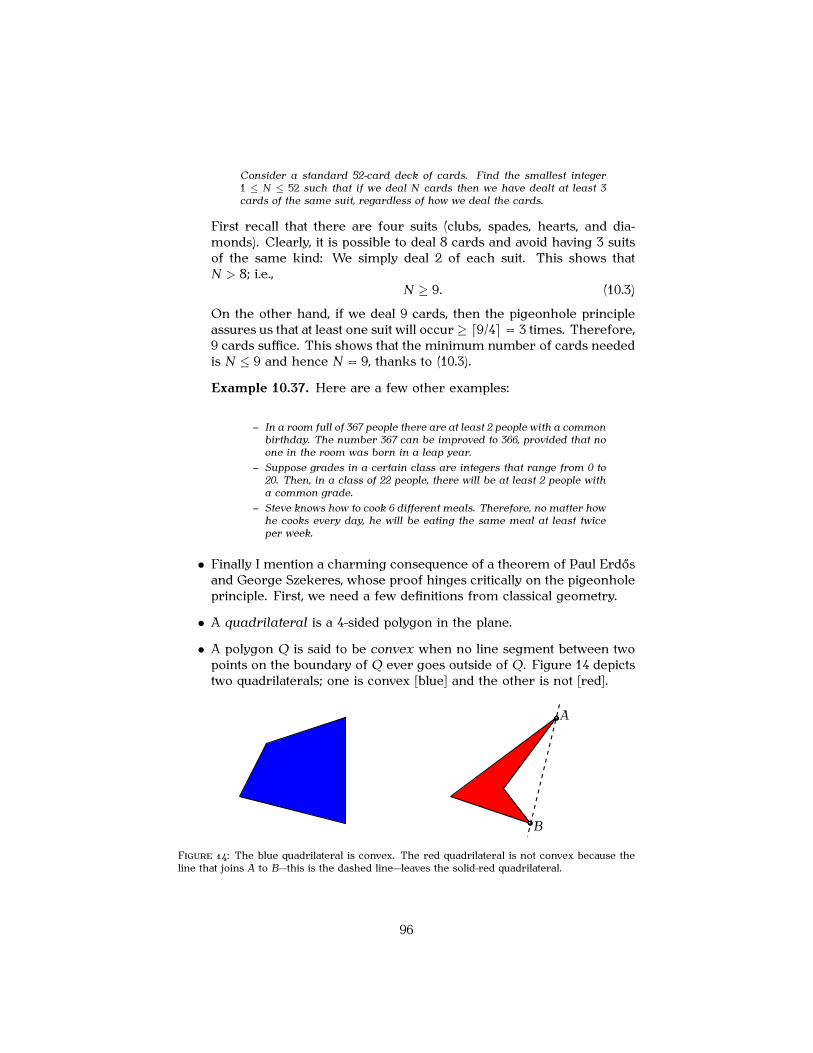
Consider a standard 52-card deck of cards. Find the smallest integer1 ≤ N ≤ 52 such that if we deal N cards then we have dealt at least 3cards of the same suit, regardless of how we deal the cards.

First recall that there are four suits (clubs, spades, hearts, and dia-monds). Clearly, it is possible to deal 8 cards and avoid having 3 suitsof the same kind: We simply deal 2 of each suit. This shows thatN > 8; i.e.,

N ≥ 9� (10.3)

On the other hand, if we deal 9 cards, then the pigeonhole principleassures us that at least one suit will occur ≥ �9/4� = 3 times. Therefore,9 cards suffice. This shows that the minimum number of cards neededis N ≤ 9 and hence N = 9, thanks to (10.3).

Example 10.37. Here are a few other examples:

– In a room full of 367 people there are at least 2 people with a commonbirthday. The number 367 can be improved to 366, provided that noone in the room was born in a leap year.

– Suppose grades in a certain class are integers that range from 0 to20. Then, in a class of 22 people, there will be at least 2 people witha common grade.

– Steve knows how to cook 6 different meals. Therefore, no matter howhe cooks every day, he will be eating the same meal at least twiceper week.

• Finally I mention a charming consequence of a theorem of Paul Erdosand George Szekeres, whose proof hinges critically on the pigeonholeprinciple. First, we need a few definitions from classical geometry.

• A quadrilateral is a 4-sided polygon in the plane.

• A polygon Q is said to be convex when no line segment between twopoints on the boundary of Q ever goes outside of Q. Figure 14 depictstwo quadrilaterals; one is convex [blue] and the other is not [red].

A

B

F����� ��: The blue quadrilateral is convex. The red quadrilateral is not convex because theline that joins A to B—this is the dashed line—leaves the solid-red quadrilateral.

96

• The following discovery of Esther Klein [1932/1933] is a consequenceof the pigeonhole principle:Proposition 10.38 (Klein, 1932/1933). Each set of 5 points in the planehas a subset of 4 points that form the vertices of a convex quadri-lateral.

F����� ��: The two figures show the same 5 planar points in two different ways in order tohighlight the content of Proposition 10.38. The blue dots of the figure on the left are 5 planarpoints. The red dots of the figure on the right form the vertices of a convex quadrilateral [alsoin red]

• There is a generalization of this fact which ultimately led to a great dealof modern mathematics. In order to descibe that generalization, firstlet � ≥ 2 be an integer and define N� to be the smallest integer � ≥ 1such that every non-degenerate �-sided polygon has the property that� of its vertices form the vertices of a convex subpolygon. If such aninteger � does not exist, then set N� := ∞.

• N� ≥ � for all � ≥ 2 because we need at least � vertices in our polygonbefore we can look for � vertices of a convex subpolygon.

• Esther Klein’s theorem [Proposition 10.38] tells us that N4 ≤ 5. And itis possible to construct a 4-sided polygon P whose vertices are not thevertices of a convex polygon [just make sure that P itself is not convex].Therefore, N4 = 5. Endre Makai (1933/1934) proved that N5 = 9.

• A few weeks hence, George Szekeres proved that N� < ∞ for all inte-gers � ≥ 2. A short while after that, Paul Erdos proved the followingremarkable result using “probabilistic methods.”Theorem 10.39 (Erdos, 1934). For every integer � ≥ 2,

N� ≤�

2� − 4� − 2

�+ 1�

• Erdos and Szekeres published their findings jointly in 1935. Erdoscalled Theorem 10.39 the happy end theorem, because Esther Kleinand George Szekeres married soon after the theorem was proved.Erdos’s ideas led to an avalanche of new mathematics that is nowadaysreferred to as Ramsey theory, combinatorial number theory, . . . .

• And so it is that our story too has come to a happy end.

97

List of Figures

1 A graphical representation of a function . . . . . . . . . . . . . . 302 A function from 3 points to 2 . . . . . . . . . . . . . . . . . . . . . 303 A plot of � (�) = �3 . . . . . . . . . . . . . . . . . . . . . . . . . . . 324 A discrete function . . . . . . . . . . . . . . . . . . . . . . . . . . . 335 The floor function . . . . . . . . . . . . . . . . . . . . . . . . . . . . 336 A function on three points. . . . . . . . . . . . . . . . . . . . . . . 347 A plot of � (�) = �2 . . . . . . . . . . . . . . . . . . . . . . . . . . . 368 A function inverse . . . . . . . . . . . . . . . . . . . . . . . . . . . 369 The composition of � and � . . . . . . . . . . . . . . . . . . . . . . 3710 A listing of Q ∩ [0 � ∞) . . . . . . . . . . . . . . . . . . . . . . . . . 4011 Navigation through Q ∩ [0 � ∞) . . . . . . . . . . . . . . . . . . . . 4012 A decorated binary tree . . . . . . . . . . . . . . . . . . . . . . . . 43

13 Rolling four Dice . . . . . . . . . . . . . . . . . . . . . . . . . . . . 8814 A convex and a non-convex quadrilateral . . . . . . . . . . . . . 9615 An illustration of the Happy End Theorem . . . . . . . . . . . . 97

98