math 141 - lecture 24: model comparisons and the f jones/courses/p24.pdfmath 141 lecture 24: model...
TRANSCRIPT

Math 141Lecture 24: Model Comparisons and The F-test
Albyn Jones1
1Library [email protected]
www.people.reed.edu/∼jones/courses/141
Albyn Jones Math 141

Nested Models
Two linear models are Nested if one (the restricted model) isobtained from the other (the full model) by setting someparameters to zero (i.e. removing terms from the model), orsome other constraint on the parameters.
We can compare nested models fit to the same dataset with theF test.
Albyn Jones Math 141

Example
# Full ModelMfull <- lm(Y ˜ X + W + Z + T,
data = MyDataSet)
# Restricted ModelMres <- lm(Y ˜ X + W, data = MyDataSet )
Fitting the restricted model is equivalent to forcing βZ = βT = 0in the full model.
Albyn Jones Math 141

Comparing Nested Models
The crucial question is whether the residual sum of squares forthe restricted model (RSSR) is substantially larger than theresidual sum of squares for the full model (RSSF ).
R. A. Fisher worked out the distribution of a ratio of the twounder the null hypothesis that the restricted model is correct,which typically corresponds to the statement that someparameters are zero.
As usual, this story depends on the residuals having a at leastan approximately normal distribution.
Albyn Jones Math 141

The F-Test
Assuming model validity, the F-ratio (F is for Fisher, by the way)
FdfN ,dfF =(RSSR − RSSF )/(dfR − dfF )
RSSF/dfF
has an F distribution with degrees of freedom (dfN ,dfF ) if therestricted model is correct.Note: dfN = dfR − dfF , and dfF and dfR are residual df from thetwo models.
Reject: if F > qf (.95,dfN ,dfF )
Note: dfR − dfF is always the number of constraints on theparameters that converts the full model to the restricted model.
Albyn Jones Math 141

The F density
0 1 2 3 4 5
0.0
0.1
0.2
0.3
0.4
0.5
0.6
0.7
F(5,20) density
X
dens
ity
Rejection Region
Albyn Jones Math 141

Analogy
0 1 2 3 4 5
0.0
0.2
0.4
0.6
0.8
X
dens
ity
F(5,20) density vs Chisq(5)/5
Fk ,n is to χ2k as tn is to N(0,1). The denominator estimates σ2.
If we knew σ2, the ratio would have a χ2 distribution.
Albyn Jones Math 141

Connection to the t Distribution: F1,k is t2k
lm(formula = ht18 ˜ ht2, data = Berkeley)
Coefficients:Estimate Std. Error t value Pr(>|t|)
(Intercept) 32.1203 26.6572 1.205 0.233ht2 1.5998 0.3031 5.278 2.2e-06---
Residual standard error: 7.572on 56 degrees of freedom
F-statistic: 27.86 on 1 and 56 DF, p-value: 2.2e-06
> 5.278ˆ2[1] 27.85728
Albyn Jones Math 141

Example, CPS wage data summary
Call:lm(formula = wage ˜ race*sex + educ + age + union,
data = CPS)
Coefficients:Estimate Std. Error t value Pr(>|t|)
(Intercept) -7.09772 1.46620 -4.841 < .001raceW 0.06191 0.89024 0.070 0.94458sexM 0.59693 1.10624 0.540 0.58970educ 0.82717 0.07405 11.170 < .001age 0.10481 0.01672 6.268 < .001unionUnion 1.59479 0.51016 3.126 0.00187raceW:sexM 1.77023 1.17363 1.508 0.13207
Albyn Jones Math 141

Plot Residuals!
●
●
●
●●
●
●●
●
●
●
●
●
●
●
●●
●
● ●●
●
●
●
●
●
●
●
●
●
●
●
●
●
●
●
●
●●
●
●
●
●
●
● ●
●
●
●
●
●
●
●
●●
●
●
●
●
● ●
●
●
●
●
●
●
●●
●
●
●
●
●●
●
●
●
●
●
●
●
●●
● ●
●
●
●●
●●
●
●
●
●
●
●
●
● ●
●
●
●
●
●
● ●
●
●
●
●
●
●
●
●
●
●●● ●
●
●●
●
●●
●
●
●
●
●
●
●
●●
●
● ●
●
●
●
●
●
●●
●
●
●●
●
●
●
●
●
●
●●
●
●
●
●
●
●
●
●
●●
●
●●●
●
●
●
●
●
●
●
●
●●
●
●
●
●
●
●
●
●
●●
●
●
●●
●
●
●
●
●
●
●
●
●
●●●●
●
●
●
●
●
●
●
●
●
●●
●●
●
●
●
●
●
●
●
●
●
●
●
●
●
●
●●
●
●
●
●
●●
●●● ●
●
●
●
●●
●
●
●
●
●
●
●
●
●●
●●
●
●●
●
●
●
●
●
●●
●
●●
●●
●
●
●
●● ●
●●
●
●●
●
●
●● ●
●
●
●
●
●
●
●
●
●
●
●
●
●
●
●●
●
●
●
●
●
●
●
●
●
●
● ●
●
●
●
●
●
●
●
● ●●●
●
●
●
●
●
●
●
●
●
●●
●
●●
●●
●
●●
●
● ● ●●
●●
●●●●
●
●
●
●
●●●●●
●
●
●
●
●
●●
●●
●● ●
●
●
●
●
●
●
●
●
●
●
●
● ●
●●
●
●
●
●
●
●
●
●
●
●
●
●●
●
●
●
●
●
●
●
●
●● ●
●
●
●●●
●
●
●
●
●
●●
● ●
●●●
● ●
●
●
●
●
●
●
●
●
●
●
● ●
●
●●
●
●
●●●
●
●
●●
●
●
●
●●
●●
●
●●
●
●
●
●
●
●
●
●●
●
●
●
●●
●
●
●
●
●
●●
●
●
●
●
●
●
●
●
●
●
●
●
●
●
●
●●
●
●
●
●● ●●
●
●
●
●
●
●
●
●
●●
●
0 5 10 15
−10
010
2030
fitted(CPS.lmf)
resi
dual
s(C
PS
.lmf)
CPS wage residuals
What Next?
Albyn Jones Math 141
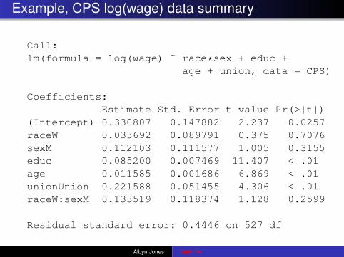
Example, CPS log(wage) data summary
Call:lm(formula = log(wage) ˜ race*sex + educ +
age + union, data = CPS)
Coefficients:Estimate Std. Error t value Pr(>|t|)
(Intercept) 0.330807 0.147882 2.237 0.0257raceW 0.033692 0.089791 0.375 0.7076sexM 0.112103 0.111577 1.005 0.3155educ 0.085200 0.007469 11.407 < .01age 0.011585 0.001686 6.869 < .01unionUnion 0.221588 0.051455 4.306 < .01raceW:sexM 0.133519 0.118374 1.128 0.2599
Residual standard error: 0.4446 on 527 df
Albyn Jones Math 141

Plot Residuals Again!
●
●●
●
●
●
● ●●
●
●●
●
●
●
●
●
●
●
●●
●
●
●
●
●
●
●
●
●
●
●
●
●
●
●
●
●●
●
●
●●
●
●
●
●
●
●
●
●
●●
● ●
●
●
●
●
● ●
●
●
●
●
●
●
●
●
●
●
●
●
●●
●
●
●
●
●
●
●
●
●
●●
● ●
●
●
●●
●
● ●
●
●
●
●
●●
●●
●
●
●
●
●
●
●
●
●
●
●
●●
●
●
●
● ●●
●●●
●
●
●
●
●
●
●
●
●
●●
●
●
●
●
●
●
●
●
●●
●
●
●●
●
●
●
●
●
●
●
●
●
●
●
●
●
●
●
●●●
●
●
● ●
●
●
●
●
●
●● ●
●
● ●
●
●
●
●
●
●
●
●●
●
●
●●
●
●
●
●
●
●
●
●
●
●●
●●
●
●
●
●
●
●
●
●
●
●●●
●
●
●
●
●
●
●
●
●
●
●
●
●
●
●
●●
●
●
●
●
●●
●●
●●
●
●
●
●
●
●
●
●
●
●
●
●
●
●
●●
●
●
●
●
●
●
●
●
●
●
●
●
●●
●
●
●
●
●
●
●
●
●
●
●●●
●
●
●
● ●
●
●
●
●
●
●
●
●
●
●
●
●
●
●●
●●
●
●
●
●
●
●
●
●
●
●●
● ●
● ●
●
●
●
●●
●●
●●
●
●
●
●
● ●
●
●●
●
●●
●
●
●
●
●●
●
●●
●
●●
●●
●●
●
●
●●
●●
●
●●
●
●
●
●
●
●●
●
●
●
● ●
●
●
●
●
●
●
●
●●
●
●
●
●
● ●
●
●●
●
●
●
●
●
●
●
●
●
●
●
●
●
●
●
●
●
●
●
●●
●● ●●● ●
●
●
●
●
●●
● ●
●
●
●
●
●
●
●
●
●
●
●
●
●
●
●
●●
●
●●
●
●
●
●●
●
●
●
●●
●
●
●
●
●
●
●
●●
●
●
●
●
●
●
●
●● ●
●●
●●
●
●
●
●
●
●
●
●
●
●
● ●
●
●
●
●
●
●
●
●
●
●●●
●
●
●●
●
●●
●
●
● ●
●
●
●
●
●
●
●
1.0 1.5 2.0 2.5 3.0
−2
−1
01
2
fitted(CPS.lmf)
resi
dual
s(C
PS
.lmf)
CPS log wage residuals
Better?
Albyn Jones Math 141

Looking for a parsimonius model?
None of the coefficients for race, sex, and the race*sexinteraction were statisticially significantly different from zero.Let’s fit a restricted model, dropping those non-significantexplanatory variables.
Albyn Jones Math 141

Example, CPS log(wage) Restricted Model
Call:lm(formula = log(wage) ˜ educ + age + union,
data = CPS)
Coefficients:Estimate Std. Error t value Pr(>|t|)
(Intercept) 0.511462 0.127785 4.003 < .01educ 0.084898 0.007694 11.034 < .01age 0.010742 0.001728 6.217 < .01unionUnion 0.260260 0.052135 4.992 < .01
Residual standard error: 0.4593 on 530 df
Albyn Jones Math 141

Model Comparison
> anova(CPS.loglmr,CPS.loglmf)Analysis of Variance Table
Model 1: log(wage) ˜ educ + age + unionModel 2: log(wage) ˜ race*sex + educ + age + unionRes.Df RSS Df Sum of Sq F Pr(>F)
1 530 111.812 527 104.16 3 7.6478 12.898 3.836e-08
Say WHAT? None of the omitted coefficients were statisticallysignificantly different from 0! How can this happen?
Albyn Jones Math 141

The Null and Alternative Hypotheses
What is H0?The restricted model is correct. Informally: the restricted modelfits as well as the full model.
Formally:H0: coefficients for the omitted terms are all 0.
Formally:H1: at least one omitted coefficient is not zero.
Albyn Jones Math 141

Important!
Individual t-tests are testing a null hypothesis for a singlecoefficient
H0 : β = 0
given we have controlled for the other variables in themodel!
Albyn Jones Math 141

What was missing?
formula = log(wage) ˜ sex + educ + age + union,data = CPS)
Coefficients:Estimate Std. Error t value Pr(>|t|)
(Intercept) 0.352998 0.126995 2.780 0.00564sexM 0.228555 0.039400 5.801 < .001educ 0.085473 0.007468 11.445 < .001age 0.011727 0.001686 6.957 < .001unionUnion 0.210191 0.051331 4.095 < .001
Albyn Jones Math 141

What happened?
The race*sex interaction was a distraction!
> cor(sex=="M",sex=="M" & race=="W")[1] 0.8638632
Strongly correlated explanatory variables can be distractors,each does part of the work of predicting the response, neitherseems important when the other is included.
Albyn Jones Math 141

Interpretation
The coefficient for the dummy variable for Males was about .23.What does that mean?
All other factors held equal, the difference between log(wage)for males and log(wage) for females is .23:
log(W ) = OtherStuff + .23 · sexM
Therefore
W = eOtherStuff+.23·sexM = eOtherStuff e.23·sexM
The dummy variable sexM is 1 for males and 0 for females, sothe difference is the multiplicative factor
e.23 ≈ 1.26
Conclusion: Males with the same education level, age andUnion status get paid about 26% more than correspondingfemales with the same covariate values.
Albyn Jones Math 141

R will try to prevent silliness
> anova(CPS.loglmr,CPS.lmf)Analysis of Variance Table
Response: log(wage)Df Sum Sq Mean Sq F value Pr(>F)
educ 1 21.481 21.4807 101.821 < .001age 1 9.898 9.8976 46.916 < .001union 1 5.257 5.2573 24.920 < .001Residuals 530 111.811 0.2110---
Warning message:In anova.lmlist(object, ...) :models with response "wage" removed becauseresponse differs from model 1
Albyn Jones Math 141

Michelson’s Data, full model
> summary(MF)Call:lm(formula = Speed ˜ Run, data = Michelson)
Coefficients:Estimate Std. Error t value Pr(>|t|)
(Intercept) 299909.00 16.60 18067.739 0.000Run2 -53.00 23.47 -2.258 0.026Run3 -64.00 23.47 -2.726 0.007Run4 -88.50 23.47 -3.770 0.000Run5 -77.50 23.47 -3.301 0.001
Albyn Jones Math 141

Michelson’s Data, restricted model
> Run1 <- Michelson$Run == 1
> summary(MR)
Call:lm(formula = Speed ˜ Run1, data = Michelson)
Coefficients:Estimate Std. Error t value Pr(>|t|)
(Intercept) 2.998e+05 8.283e+00 36197.63 < 2e-16Run1TRUE 7.075e+01 1.852e+01 3.82 0.000234
Albyn Jones Math 141

Model Comparison!
> anova(MR,MF)Analysis of Variance Table
Model 1: Speed ˜ Run1Model 2: Speed ˜ RunRes.Df RSS Df Sum of Sq F Pr(>F)
1 98 5379352 95 523510 3 14425 0.8726 0.4582
What was H0, and what do we conclude?
Albyn Jones Math 141

Summary
The F test compares nested models fit to the same dataset.
It allows us to test hypotheses involving multiple parameterssimultaneously.
If you wish to conclude that a collection of coefficients are allzero, or none of a subset of your explanatory variables predictthe response, an F-test is the appropriate tool.
Albyn Jones Math 141