materials engineering, science, processing and design
DESCRIPTION
Materials engineering, science, processing and designTRANSCRIPT
MaterialsEngineering, Science, Processing and Design
Michael Ashby, Hugh Shercliff and David Cebon
University of Cambridge, UK
AMSTERDAM • BOSTON • HEIDELBERG • LONDON • NEW YORK • OXFORD
PARIS • SAN DIEGO • SAN FRANCISCO • SINGAPORE • SYDNEY • TOKYOButterworth-Heinemann is an imprint of Elsevier
Prelims-H8391 1/16/07 12:16 PM Page i

Butterworth-Heinemann is an imprint of ElsevierLinacre House, Jordan Hill, Oxford OX2 8DP30 Corporate Drive, Suite 400, Burlington, MA 01803
First edition 2007
Copyright © 2007, Michael Ashby, Hugh Shercliff and David Cebon. Published by Elsevier Ltd. All rights reserved.
The right of Michael Ashby, Hugh Shercliff and David Cebon to be identified as the authors of this work has beenasserted in accordance with the Copyright, Designs and Patents Act 1988
No part of this publication may be reproduced, stored in a retrieval system, or transmitted in any form or by any means electronic, mechanical, photocopying, recording or otherwise without the prior written permission of the publisher
Permissions may be sought directly from Elsevier’s Science & Technology Rights Department in Oxford, UK: phone (44) (0) 1865 843830; fax: (44) (0) 1865 853333; email: [email protected] you can submit your request online by visiting the Elsevier web site at http://elsevier.com/locate/permissions, and selecting Obtaining permission to use Elsevier material
NoticeNo responsibility is assumed by the publisher for any injury and/or damage to persons or property as a matter of products liability, negligence or otherwise, or from any use or operation of any methods, products, instructions or ideas contained in the material herein. Because of rapid advances in the medical sciences,in particular, independent verification of diagnoses and drug dosages should be made
British Library Cataloguing in Publication DataA catalogue record for this book is available from the British Library
Library of Congress Cataloging-in-Publication DataA catalog record for this book is available from the Library of Congress
ISBN-13: 978-0-7506-8391-3ISBN-10: 0-7506-8391-0
For information on all Butterworth-Heinemann publicationsvisit our web site at http://books.elsevier.com
Typeset by Charon Tec Ltd (A Macmillan Company), Chennai, India.www.charontec.com
Printed and bound in the UK
07 08 09 10 10 9 8 7 6 5 4 3 2 1
Prelims-H8391 1/16/07 12:16 PM Page ii

Contents
Preface ixAcknowledgements xiResources that accompany this book xii
Chapter 1 Introduction: materials—history and character 11.1 Materials, processes and choice 21.2 Material properties 41.3 Design-limiting properties 91.4 Summary and conclusions 101.5 Further reading 101.6 Exercises 10
Chapter 2 Family trees: organizing materials and processes 132.1 Introduction and synopsis 142.2 Getting materials organized: the materials tree 142.3 Organizing processes: the process tree 182.4 Process–property interaction 212.5 Material property charts 222.6 Computer-aided information management for materials and processes 242.7 Summary and conclusions 252.8 Further reading 262.9 Exercises 262.10 Exploring design using CES 282.11 Exploring the science with CES Elements 28
Chapter 3 Strategic thinking: matching material to design 293.1 Introduction and synopsis 303.2 The design process 303.3 Material and process information for design 343.4 The strategy: translation, screening, ranking and documentation 363.5 Examples of translation 393.6 Summary and conclusions 433.7 Further reading 433.8 Exercises 443.9 Exploring design using CES 46
Prelims-H8391 1/16/07 12:16 PM Page iii

Chapter 4 Stiffness and weight: density and elastic moduli 474.1 Introduction and synopsis 484.2 Density, stress, strain and moduli 484.3 The big picture: material property charts 564.4 The science: what determines density and stiffness? 584.5 Manipulating the modulus and density 694.6 Summary and conclusions 734.7 Further reading 744.8 Exercises 744.9 Exploring design with CES 774.10 Exploring the science with CES Elements 78
Chapter 5 Flex, sag and wobble: stiffness-limited design 815.1 Introduction and synopsis 825.2 Standard solutions to elastic problems 825.3 Material indices for elastic design 895.4 Plotting limits and indices on charts 955.5 Case studies 995.6 Summary and conclusions 1065.7 Further reading 1075.8 Exercises 1075.9 Exploring design with CES 1095.10 Exploring the science with CES Elements 109
Chapter 6 Beyond elasticity: plasticity, yielding and ductility 1116.1 Introduction and synopsis 1126.2 Strength, plastic work and ductility: definition and measurement 1126.3 The big picture: charts for yield strength 1166.4 Drilling down: the origins of strength and ductility 1186.5 Manipulating strength 1276.6 Summary and conclusions 1356.7 Further reading 1366.8 Exercises 1376.9 Exploring design with CES 1386.10 Exploring the science with CES Elements 138
Chapter 7 Bend and crush: strength-limited design 1417.1 Introduction and synopsis 1427.2 Standard solutions to plastic problems 1427.3 Material indices for yield-limited design 1497.4 Case studies 1547.5 Summary and conclusions 1587.6 Further reading 159
iv Contents
Prelims-H8391 1/16/07 12:16 PM Page iv
7.7 Exercises 1597.8 Exploring design with CES 161
Chapter 8 Fracture and fracture toughness 1638.1 Introduction and synopsis 1648.2 Strength and toughness 1648.3 The mechanics of fracture 1668.4 Material property charts for toughness 1728.5 Drilling down: the origins of toughness 1748.6 Manipulating properties: the strength–toughness trade-off 1788.7 Summary and conclusions 1818.8 Further reading 1818.9 Exercises 1828.10 Exploring design with CES 1838.11 Exploring the science with CES Elements 183
Chapter 9 Shake, rattle and roll: cyclic loading, damage and failure 1859.1 Introduction and synopsis 1869.2 Vibration and resonance: the damping coefficient 1869.3 Fatigue 1879.4 Charts for endurance limit 1949.5 Drilling down: the origins of damping and fatigue 1959.6 Manipulating resistance to fatigue 1969.7 Summary and conclusions 1989.8 Further reading 1999.9 Exercises 1999.10 Exploring design with CES 202
Chapter 10 Keeping it all together: fracture-limited design 20310.1 Introduction and synopsis 20410.2 Standard solutions to fracture problems 20410.3 Material indices for fracture-safe design 20510.4 Case studies 20910.5 Summary and conclusions 22010.6 Further reading 22110.7 Exercises 22110.8 Exploring design with CES 224
Chapter 11 Rub, slither and seize: friction and wear 22711.1 Introduction and synopsis 22811.2 Tribological properties 22811.3 Charting friction and wear 22911.4 The physics of friction and wear3 231
Contents v
Prelims-H8391 1/16/07 12:16 PM Page v

11.5 Design and selection: materials to manage friction and wear 23511.6 Summary and conclusions 24011.7 Further reading 24111.8 Exercises 24111.9 Exploring design with CES 243
Chapter 12 Agitated atoms: materials and heat 24512.1 Introduction and synopsis 24612.2 Thermal properties: definition and measurement 24612.3 The big picture: thermal property charts 24912.4 Drilling down: the physics of thermal properties 25112.5 Manipulating thermal properties 25712.6 Design to exploit thermal properties 25812.7 Summary and conclusions 26812.8 Further reading 26912.9 Exercises 27012.10 Exploring design with CES 27112.11 Exploring the science with CES Elements 272
Chapter 13 Running hot: using materials at high temperatures 27513.1 Introduction and synopsis 27613.2 The temperature dependence of material properties 27613.3 Charts for creep behavior 28113.4 The science: diffusion and creep 28413.5 Materials to resist creep 29313.6 Design to cope with creep 29613.7 Summary and conclusions 30413.8 Further reading 30513.9 Exercises 30513.10 Exploring design with CES 30813.11 Exploring the science with CES Elements 308
Chapter 14 Conductors, insulators and dielectrics 31114.1 Introduction and synopsis 31214.2 Conductors, insulators and dielectrics 31314.3 Charts for electrical properties 31714.4 Drilling down: the origins and manipulation of electrical properties 32014.5 Design: using the electrical properties of materials 33114.6 Summary and conclusions 33814.7 Further reading 33814.8 Exercises 33914.9 Exploring design with CES 34114.10 Exploring the science with CES Elements 343
vi Contents
Prelims-H8391 1/16/07 12:16 PM Page vi

Chapter 15 Magnetic materials 34515.1 Introduction and synopsis 34615.2 Magnetic properties: definition and measurement 34615.3 Charts for magnetic properties 35115.4 Drilling down: the physics and manipulation of magnetic properties 35315.5 Materials selection for magnetic design 35815.6 Summary and conclusions 36315.7 Further reading 36315.8 Exercises 36415.9 Exploring design with CES 36515.10 Exploring the science with CES Elements 366
Chapter 16 Materials for optical devices 36716.1 Introduction and synopsis 36816.2 The interaction of materials and radiation 36816.3 Charts for optical properties 37316.4 Drilling down: the physics and manipulation of optical properties 37516.5 Optical design 38116.6 Summary and conclusions 38216.7 Further reading 38316.8 Exercises 38316.9 Exploring design with CES 38416.10 Exploring the science with CES Elements 385
Chapter 17 Durability: oxidation, corrosion and degradation 38717.1 Introduction and synopsis 38817.2 Oxidation, flammability and photo-degradation 38817.3 Oxidation mechanisms 39017.4 Making materials that resist oxidation 39217.5 Corrosion: acids, alkalis, water and organic solvents 39517.6 Drilling down: mechanisms of corrosion 39617.7 Fighting corrosion 40117.8 Summary and conclusions 40417.9 Further reading 40517.10 Exercises 40517.11 Exploring design with CES 40617.12 Exploring the science with CES Elements 407
Chapter 18 Heat, beat, stick and polish: manufacturing processes 40918.1 Introduction and synopsis 41018.2 Process selection in design 41018.3 Process attributes: material compatibility 41318.4 Shaping processes: attributes and origins 414
Contents vii
Prelims-H8391 1/16/07 12:16 PM Page vii

18.5 Joining processes: attributes and origins 42318.6 Surface treatment (finishing) processes: attributes and origins 42618.7 Estimating cost for shaping processes 42718.8 Computer-aided process selection 43218.9 Case studies 43418.10 Summary and conclusions 44318.11 Further reading 44418.12 Exercises 44518.13 Exploring design with CES 44618.14 Exploring the science with CES Elements 447
Chapter 19 Follow the recipe: processing and properties 44919.1 Introduction and synopsis 45019.2 Microstructure of materials 45019.3 Microstructure evolution in processing 45419.4 Processing for properties 46219.5 Case studies 46419.6 Making hybrid materials 47219.7 Summary and conclusions 47419.8 Further reading 47519.9 Exercises 47619.10 Exploring design with CES 477
Chapter 20 Materials, processes and the environment 47920.1 Introduction and synopsis 48020.2 Material consumption and its growth 48020.3 The material life cycle and criteria for assessment 48320.4 Definitions and measurement: embodied energy, process
energy and end of life potential 48420.5 Charts for embodied energy 49020.6 Design: selecting materials for eco-design 49320.7 Summary and conclusions 49720.8 Appendix: some useful quantities 49820.9 Further reading 49820.10 Exercises 49920.11 Exploring design with CES 501
Index 503
viii Contents
Prelims-H8391 1/16/07 12:16 PM Page viii

Preface
Science-led or Design-led? Two approaches to materials teaching
Most things can be approached in more than one way. In teaching this is especially true. The wayto teach a foreign language, for example, depends on the way the student wishes to use it—to readthe literature, say, or to find accommodation, order meals and buy beer. So it is with the teachingof this subject.
The traditional approach to it starts with fundamentals: the electron, the atom, atomic bonding,and packing, crystallography and crystal defects. Onto this is built alloy theory, the kinetics ofphase transformation and the development of microstructure on scales made visible by electron andoptical microscopes. This sets the stage for the understanding and control of properties at the mil-limeter or centimeter scale at which they are usually measured. The approach gives little emphasisto the behavior of structures, methods for material selection, and design.
The other approach is design-led. The starting point is the need: the requirements that materialsmust meet if they are to perform properly in a given design. To match materials to designs requiresa perspective of the range of properties they offer and the other information that will be needed aboutthem to enable successful selection. Once the importance of a property is established there is goodreason to ‘drill down’, so to speak, to examine the science that lies behind it—valuable because anunderstanding of the fundamentals itself informs material choice and usage.
There is sense in both approaches. It depends on the way the student wishes to use the information.If the intent is scientific research, the first is the logical way to go. If it is engineering design, the sec-ond makes better sense. This book follows the second.
What is different about this book?
There are many books about the science of engineering materials and many more about design.What is different about this one?
First, a design-led approach specifically developed to guide material selection and manipulation.The approach is systematic, leading from design requirements to a prescription for optimized materialchoice. The approach is illustrated by numerous case studies. Practice in using it is provided byExercises.
Second, an emphasis on visual communication and a unique graphical presentation of materialproperties as material property charts. These are a central feature of the approach, helpful both inunderstanding the origins of properties, their manipulation and their fundamental limits, as well asproviding a tool for selection and for understanding the ways in which materials are used.
Third, its breadth. We aim here to present the properties of materials, their origins and the waythey enter engineering design. A glance at the Contents pages will show sections dealing with:
• Physical properties• Mechanical characteristics• Thermal behavior
Prelims-H8391 1/16/07 12:16 PM Page ix
• Electrical, magnetic and optical response• Durability• Processing and the way it influences properties• Environmental issues
Throughout we aim for a simple, straightforward presentation, developing the materials science asfar as is it helpful in guiding engineering design, avoiding detail where this does not contribute tothis end.
And fourth, synergy with the Cambridge Engineering Selector (CES)1—a powerful and widelyused PC-based software package that is both a source of material and process information and atool that implements the methods developed in this book. The book is self-contained: access to thesoftware is not a prerequisite for its use. Availability of the CES EduPack software suite enhancesthe learning experience. It allows realistic selection studies that properly combine multiple con-straints on material and processes attributes, and it enables the user to explore the ways in whichproperties are manipulated.
The CES EduPack contains an additional tool to allow the science of materials to be explored inmore depth. The CES Elements database stores fundamental data for the physical, crystallographic,mechanical, thermal, electrical, magnetic and optical properties of all 111 elements. It allows inter-relationships between properties, developed in the text, to be explored in depth.
The approach is developed to a higher level in two further textbooks, the first relating to mechan-ical design2, the second to industrial design3.
x Preface
1 The CES EduPack 2007, Granta Design Ltd., Rustat House, 62 Clifton Court, Cambridge CB1 7EG, UK, www.grantadesign.com.
2 Ashby, M.F. (2005), Materials Selection in Mechanical Design, 3rd edition, Butterworth-Heinemann, Oxford, UK,Chapter 4. ISBN 0-7506-6168-2. (A more advanced text that develops the ideas presented here in greater depth.)
3 Ashby, M.F. and Johnson, K. (2002) Materials and Design—The Art and Science of Material Selection in ProductDesign, Butterworth-Heinemann, Oxford, UK. ISBN 0-7506-5554-2. (Materials and processes from an aestheticpoint of view, emphasizing product design.)
Prelims-H8391 1/16/07 12:16 PM Page x

Acknowledgements
No book of this sort is possible without advice, constructive criticism and ideas from others. Numerouscolleagues have been generous with their time and thoughts. We would particularly like to recog-nize suggestions made by Professors Mick Brown, Archie Campbell, Dave Cardwell, Ken Wallace andKen Johnson, all of Cambridge University, and acknowledge their willingness to help. Equally valu-able has been the contribution of the team at Granta Design, Cambridge, responsible for the devel-opment of the CES software that has been used to make the material property charts that are afeature of this book.
Prelims-H8391 1/16/07 12:16 PM Page xi

Resources that accompany this book
Exercises
Each chapter ends with exercises of three types: the first rely only on information, diagrams anddata contained in the book itself; the second makes use of the CES software in ways that use themethods developed here, and the third explores the science more deeply using the CES Elementsdatabase that is part of the CES system.
Instructor’s manual
The book itself contains a comprehensive set of exercises. Worked-out solutions to the exercises arefreely available to teachers and lecturers who adopt this book. To access this material online pleasevisit http://textbooks.elsevier.com and follow the instructions on screen.
Image Bank
The Image Bank provides adopting tutors and lecturers with jpegs and gifs of the figures from thebook that may be used in lecture slides and class presentations. To access this material please visithttp://textbooks.elsevier.com and follow the instructions on screen.
The CES EduPack
CES EduPack is the software-based package to accompany this book, developed by Michael Ashbyand Granta Design. Used together, Materials: Engineering, Science, Processing and Design and CESEduPack provide a complete materials, manufacturing and design course. For further informationplease see the last page of this book, or visit www.grantadesign.com.
Prelims-H8391 1/16/07 12:16 PM Page xii

Chapter 1Introduction: materials—
history and character
Chapter contents
1.1 Materials, processes and choice 21.2 Material properties 41.3 Design-limiting properties 91.4 Summary and conclusions 101.5 Further reading 101.6 Exercises 10
Professor James Stuart, the first Professorof Engineering at Cambridge.
Ch01-H8391 1/16/07 6:40 PM Page 1
2 Chapter 1 Introduction: materials—history and character
1.1 Materials, processes and choice
Engineers make things. They make them out of materials. The materials haveto support loads, to insulate or conduct heat and electricity, to accept or rejectmagnetic flux, to transmit or reflect light, to survive in often-hostile sur-roundings, and to do all this without damage to the environment or costingtoo much.
And there is the partner in all this. To make something out of a material youalso need a process. Not just any process—the one you choose has to be com-patible with the material you plan to use. Sometimes it is the process that is thedominant partner and a material-mate must be found that is compatible withit. It is a marriage. Compatibility is not easily found—many marriages fail—and material failure can be catastrophic, with issues of liability and compensa-tion. This sounds like food for lawyers, and sometimes it is: some specialistsmake their living as expert witnesses in court cases involving failed materials.But our aim here is not contention; rather, it is to give you a vision of the mate-rials universe (since, even on the remotest planets you will find the same ele-ments) and of the universe of processes, and to provide methods and tools forchoosing them to ensure a happy, durable union.
But, you may say, engineers have been making things out of materials forcenturies, and successfully so—think of Isambard Kingdom Brunel, ThomasTelford, Gustave Eiffel, Henry Ford, Karl Benz and Gottlieb Daimler, theWright brothers. Why do we need new ways to choose them? A little historyhelps here. Glance at the portrait with which this chapter starts: it shows JamesStuart, the first Professor of Engineering at Cambridge University from 1875 to1890 (note the cigar). In his day the number of materials available to engineerswas small—a few hundred at most. There were no synthetic polymers—thereare now over 45 000 of them. There were no light alloys (aluminum was firstestablished as an engineering material only in the 20th century)—now there arethousands. There were no high-performance composites—now there are hun-dreds of them. The history is developed further in Figure 1.1, the time-axis ofwhich spans 10 000 years. It shows roughly when each of the main classes ofmaterials first evolved. The time-scale is nonlinear—almost all the materials weuse today were developed in the last 100 years. And this number is enormous:over 160 000 materials are available to today’s engineer, presenting us with aproblem that Professor Stuart did not have: that of optimally selecting fromthis huge menu. With the ever-increasing drive for performance, economy andefficiency, and the imperative to avoid damage to the environment, making theright choice becomes very important. Innovative design means the imaginativeexploitation of the properties offered by materials.
These properties, today, are largely known and documented in handbooks;one such—the ASM Materials Handbook—runs to 22 fat volumes, and it is oneof many. How are we to deal with this vast body of information? Fortunatelyanother thing has changed since Prof. Stuart’s day: we now have digital informa-tion storage and manipulation. Computer-aided design is now a standard part
Ch01-H8391 1/16/07 6:40 PM Page 2

1.1 Materials, processes and choice 3
of an engineer’s training, and it is backed up by widely available packages forsolid modeling, finite-element analysis, optimization, and for material andprocess selection. Software for the last of these—the selection of materials andprocesses—draws on databases of the attributes of materials and processes, doc-umenting their mutual compatibility, and allows them to be searched and dis-played in ways that enable selections that best meet the requirements of a design.
If you travel by foot, bicycle or car, you take a map. The materials landscape,like the terrestrial one, can be complex and confusing; maps, here, are also a goodidea. This text presents a design-led approach to materials and manufacturing
5000BC10000BC 0 1000 1500 1800 1900 1940 1960 1980 1990 2000 2010
5000BC10000BC 0 1000 1500 1800 1900 1940 1960 1980 1990 2000 2010
Date
Gold CopperBronze
Iron Cast iron
Wood
SkinsFibers
GluesRubber
Straw-Brick Paper
Bakelite
StoneFlint
Pottery
GlassCement Refractories Portland
cementFusedsilica
Pyro-cerams
C-steelsAlloy steels
AluminumSuper-alloys
Titanium
Zirconium
Nylon
PE PMMA
AcrylicsPCPS
PP
Cermets
EpoxiesPolyesters
Technical ceramics:Al2O3, SiC, Si3N4, PSZ etc
GFRPCFRP
Kevlar-FRP
compositesMetal–matrix
Ceramic composites
High-moduluspolymers
High-temperaturepolymers: PEEK
Glassy metalsAl–Lithium alloys
Microalloyed steelsTin
MagnesiumMetal foams
PTFE
Metals
Polymers &elastomers
Ceramics &glasses
Hybrids
Neanderthalman
JuliusCaesar
Henry VIIIof England
Queen Victoria
FranklinRoosevelt
John F.Kennedy
George W.Bush
Figure 1.1 The development of materials over time. The materials of pre-history, on theleft, all occur naturally; the challenge for the engineers of that era was one ofshaping them. The development of thermochemistry and (later) of polymerchemistry enabled man-made materials, shown in the colored zones. Three—stone, bronze and iron—were of such importance that the era of theirdominance is named after them.
Ch01-H8391 1/16/07 6:40 PM Page 3

processes that makes use of maps: novel graphics to display the world of mate-rials and processes in easily accessible ways. They present the properties ofmaterials in ways that give a global view, that reveal relationships betweenproperties and that enable selection.
1.2 Material properties
So what are these properties? Some, like density (mass per unit volume) andprice (the cost per unit volume or weight) are familiar enough, but others arenot, and getting them straight is essential. Think first of those that have to dowith carrying load safely—the mechanical properties.
Mechanical propertiesA steel ruler is easy to bend elastically—‘elastic’ means that it springs backwhen released. Its elastic stiffness (here, resistance to bending) is set partly byits shape—thin strips are easy to bend—and partly by a property of the steelitself: its elastic modulus, E. Materials with high E, like steel, are intrinsicallystiff; those with low E, like polyethylene, are not. Figure 1.2(b) illustrates theconsequences of inadequate stiffness.
The steel ruler bends elastically, but if it is a good one, it is hard to give it apermanent bend. Permanent deformation has to do with strength, not stiffness.The ease with which a ruler can be permanently bent depends, again, on itsshape and on a different property of the steel—its yield strength, σy. Materialswith large σy, like titanium alloys, are hard to deform permanently even thoughtheir stiffness, coming from E, may not be high; those with low σy, like lead,can be deformed with ease. When metals deform, they generally get stronger(this is called ‘work hardening’), but there is an ultimate limit, called the tensilestrength, σts, beyond which the material fails (the amount it stretches before itbreaks is called the ductility). Figure 1.2(c) gives an idea of the consequences ofinadequate strength.
So far so good. One more. If the ruler were made not of steel but of glass orof PMMA (Plexiglas, Perspex), as transparent rulers are, it is not possible tobend it permanently at all. The ruler will fracture suddenly, without warning,before it acquires a permanent bend. We think of materials that break in thisway as brittle, and materials that do not as tough. There is no permanent defor-mation here, so σy is not the right property. The resistance of materials tocracking and fracture is measured instead by the fracture toughness, K1c. Steelsare tough—well, most are (steels can be made brittle)—they have a high K1c.Glass epitomizes brittleness; it has a very low K1c. Figure 1.2(d) suggests conse-quences of inadequate fracture and toughness.
We started with the material property density, mass per unit volume, symbolρ. Density, in a ruler, is irrelevant. But for almost anything that moves, weightcarries a fuel penalty, modest for automobiles, greater for trucks and trains,greater still for aircraft, and enormous in space vehicles. Minimizing weight has
4 Chapter 1 Introduction: materials—history and character
Ch01-H8391 1/16/07 6:40 PM Page 4
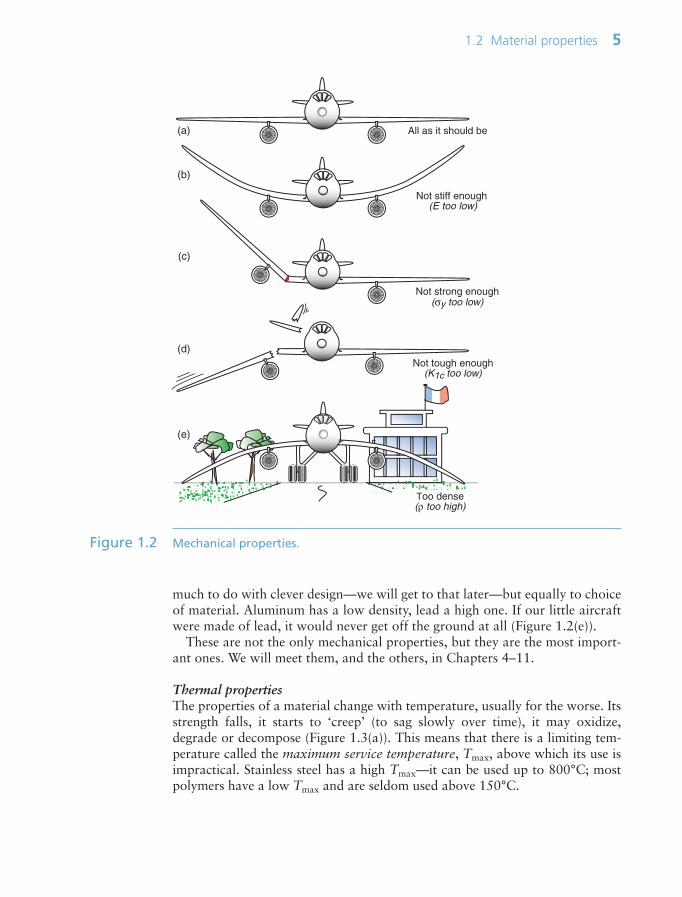
much to do with clever design—we will get to that later—but equally to choiceof material. Aluminum has a low density, lead a high one. If our little aircraftwere made of lead, it would never get off the ground at all (Figure 1.2(e)).
These are not the only mechanical properties, but they are the most import-ant ones. We will meet them, and the others, in Chapters 4–11.
Thermal propertiesThe properties of a material change with temperature, usually for the worse. Itsstrength falls, it starts to ‘creep’ (to sag slowly over time), it may oxidize,degrade or decompose (Figure 1.3(a)). This means that there is a limiting tem-perature called the maximum service temperature, Tmax, above which its use isimpractical. Stainless steel has a high Tmax—it can be used up to 800°C; mostpolymers have a low Tmax and are seldom used above 150°C.
1.2 Material properties 5
Not stiff enough (E too low)
All as it should be
Not strong enough(σy too low)
Not tough enough(K1c too low)
Too dense(ρ too high)
(a)
(b)
(c)
(d)
(e)
Figure 1.2 Mechanical properties.
Ch01-H8391 1/16/07 6:40 PM Page 5

Most materials expand when they are heated, but by differing amountsdepending on their thermal expansion coefficient, α. The expansion is small,but its consequences can be large. If, for instance, a rod is constrained, as inFigure 1.3(b), and then heated, expansion forces the rod against the con-straints, causing it to buckle. Railroad track buckles in this way if provision isnot made to cope with it.
Some materials—metals, for instance—feel cold; others—like woods—feelwarm. This feel has to do with two thermal properties of the material: thermalconductivity and heat capacity. The first, thermal conductivity, λ, measures therate at which heat flows through the material when one side is hot and theother cold. Materials with high λ are what you want if you wish to conductheat from one place to another, as in cooking pans, radiators and heat exchang-ers; Figure 1.3(c) suggests consequences of high and low λ for the cooking ves-sel. But low λ is useful too—low λ materials insulate homes, reduce the energyconsumption of refrigerators and freezers, and enable space vehicles to re-enterthe earth’s atmosphere.
6 Chapter 1 Introduction: materials—history and character
Low conductivity λ(c) High conductivity λ
Low T-diffusivity a(d) High T-diffusivity a
Low expansion coefficient α(b) High expansion coefficient α
W W
Low service temperature Tmax(a) High service temperature Tmax
Figure 1.3 Thermal properties.
Ch01-H8391 1/16/07 6:40 PM Page 6
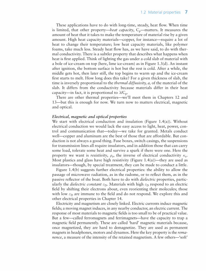
These applications have to do with long-time, steady, heat flow. When timeis limited, that other property—heat capacity, Cp—matters. It measures theamount of heat that it takes to make the temperature of material rise by a givenamount. High heat capacity materials—copper, for instance—require a lot ofheat to change their temperature; low heat capacity materials, like polymerfoams, take much less. Steady heat flow has, as we have said, to do with ther-mal conductivity. There is a subtler property that describes what happens whenheat is first applied. Think of lighting the gas under a cold slab of material witha bole of ice-cream on top (here, lime ice-cream) as in Figure 1.3(d). An instantafter ignition, the bottom surface is hot but the rest is cold. After a while, themiddle gets hot, then later still, the top begins to warm up and the ice-creamfirst starts to melt. How long does this take? For a given thickness of slab, thetime is inversely proportional to the thermal diffusivity, a, of the material of theslab. It differs from the conductivity because materials differ in their heatcapacity—in fact, it is proportional to λ/Cp.
There are other thermal properties—we’ll meet them in Chapters 12 and13—but this is enough for now. We turn now to matters electrical, magneticand optical.
Electrical, magnetic and optical propertiesWe start with electrical conduction and insulation (Figure 1.4(a)). Withoutelectrical conduction we would lack the easy access to light, heat, power, con-trol and communication that—today—we take for granted. Metals conductwell—copper and aluminum are the best of those that are affordable. But con-duction is not always a good thing. Fuse boxes, switch casings, the suspensionsfor transmission lines all require insulators, and in addition those that can carrysome load, tolerate some heat and survive a spark if there were one. Here theproperty we want is resistivity, ρe, the inverse of electrical conductivity κe.Most plastics and glass have high resistivity (Figure 1.4(a))—they are used asinsulators—though, by special treatment, they can be made to conduct a little.
Figure 1.4(b) suggests further electrical properties: the ability to allow thepassage of microwave radiation, as in the radome, or to reflect them, as in thepassive reflector of the boat. Both have to do with dielectric properties, partic-ularly the dielectric constant εD. Materials with high εD respond to an electricfield by shifting their electrons about, even reorienting their molecules; thosewith low εD are immune to the field and do not respond. We explore this andother electrical properties in Chapter 14.
Electricity and magnetism are closely linked. Electric currents induce magneticfields; a moving magnet induces, in any nearby conductor, an electric current. Theresponse of most materials to magnetic fields is too small to be of practical value.But a few—called ferromagnets and ferrimagnets—have the capacity to trap amagnetic field permanently. These are called ‘hard’ magnetic materials because,once magnetized, they are hard to demagnetize. They are used as permanentmagnets in headphones, motors and dynamos. Here the key property is the rema-nence, a measure of the intensity of the retained magnetism. A few others—‘soft’
1.2 Material properties 7
Ch01-H8391 1/16/07 6:40 PM Page 7

magnet materials—are easy to magnetize and demagnetize. They are the materi-als of transformer cores and the deflection coils of a TV tube. They have thecapacity to conduct a magnetic field, but not retain it permanently (Figure 1.4(c)).For these a key property is the saturation magnetization, which measures howlarge a field the material can conduct. These we meet again in Chapter 15.
Materials respond to light as well as to electricity and magnetism—hardlysurprising, since light itself is an electromagnetic wave. Materials that areopaque reflect light; those that are transparent refract it, and some have theability to absorb some wavelengths (colors) while allowing others to pass freely(Figure 1.4(d)). These are explored in more depth in Chapter 16.
Chemical propertiesProducts often have to function in hostile environments, exposed to corrosive flu-ids, to hot gases or to radiation. Damp air is corrosive, so is water; the sweat ofyour hand is particularly corrosive, and of course there are far more aggressiveenvironments than these. If the product is to survive for its design life it must bemade of materials—or at least coated with materials—that can tolerate the sur-roundings in which they operate. Figure 1.5 illustrates some of the commonest ofthese: fresh and salt water, acids and alkalis, organic solvents, oxidizing flames
8 Chapter 1 Introduction: materials—history and character
ON
OFF
N S
(a) Low resistivity ρe High resistivity ρe
(b) Low dielectric response High dielectric response
(c) ‘Hard’ magnetic behavior Soft magnetic behavior
(d) Refraction Absorption
Figure 1.4 Electrical, magnetic and optical properties.
Ch01-H8391 1/16/07 6:40 PM Page 8

and ultraviolet radiation. We regard the intrinsic resistance of a material to eachof these as material properties, measured on a scale of 1 (very poor) to 5 (verygood). Chapter 17 deals with the material durability.
1.3 Design-limiting properties
The performance of a component is limited by certain of the properties of thematerials of which it is made. This means that, to achieve a desired level of performance, the values of the design-limiting properties must meet certain targets—those that fail to do so are not suitable. In the cartoon of Figure 1.2,stiffness, strength and toughness are design limiting—if any one of them weretoo low, the plane won’t fly. In the design of power transmission lines electricalresistivity is design limiting; in the design of a camera lens, it is optical qualityand refractive index.
Materials are chosen by identifying the design-limiting properties and apply-ing limits to them, screening out those that do not meet the limits (Chapter 3).
1.3 Design-limiting properties 9
NITRICACID
PETROL
(a) Fresh water (b) Salt water
(c) Acids and alkalis (d) Organic solvents
(e) Oxidation (f) UV radiation
Figure 1.5 Chemical properties: resistance to water, acids, alkalis, organic solvents,oxidation and radiation.
Ch01-H8391 1/16/07 6:40 PM Page 9
Processes, too, have properties, although we have not met them yet. These toocan be design limiting, leading to a parallel scheme for choosing viableprocesses (Chapters 18 and 19).
1.4 Summary and conclusions
Engineering design depends on materials that are shaped, joined and finishedby processes. Design requirements define the performance required of the mate-rials, expressed as target values for certain design-limiting properties. A mate-rial is chosen because it has properties that meet these targets and is compatiblewith the processes required to shape, join and finish it.
This chapter introduced some of the design-limiting properties: physicalproperties (like density), mechanical properties (like modulus and yield strength)and functional properties (those describing the thermal, electrical, magneticand optical behavior). We examine all of these in more depth in the chaptersthat follow, but those just introduced are enough to be going on with. We turnnow to the materials themselves: the families, the classes and the members.
1.5 Further reading
The history and evolution of materials
A History of Technology (1954–2001) (21 volumes), edited by Singer, C., Holmyard, E.J.,Hall, A.R., Williams, T.I. and Hollister-Short, G. Oxford University Press, Oxford, UK. ISSN 0307-5451. (A compilation of essays on aspects of technology, includingmaterials.)
Delmonte, J. (1985) Origins of Materials and Processes, Technomic PublishingCompany, Pennsylvania, USA. ISBN 87762-420-8. (A compendium of informationabout materials in engineering, documenting the history.)
Tylecoate, R.F. (1992) A History of Metallurgy, 2nd edition, The Institute of Materials,London, UK. ISBN 0-904357-066. (A total-immersion course in the history of theextraction and use of metals from 6000 BC to 1976, told by an author with forensictalent and love of detail.)
1.6 Exercises
10 Chapter 1 Introduction: materials—history and character
Exercise E1.1 Use Google to research the history and uses of one of the following materials:
• Tin• Glass• Cement
Ch01-H8391 1/16/07 6:40 PM Page 10

1.6 Exercises 11
• Titanium• Carbon fiber.
Present the result as a short report of about 100–200 words (roughly half apage).
Exercise E1.2 What is meant by the design-limiting properties of a material in a given appli-cation?
Exercise E1.3 There have been many attempts to manufacture and market plastic bicycles. Allhave been too flexible. Which design-limiting property is insufficiently large?
Exercise E1.4 What, in your judgement, are the design-limiting properties for the materialfor the blade of a knife that will be used to gut fish?
Exercise E1.5 What, in your judgement, are the design-limiting properties for the materialof an oven glove?
Exercise E1.6 What, in your judgement, are the design-limiting properties for the materialof an electric lamp filament?
Exercise E1.7 A material is needed for a tube to carry fuel from the fuel tank to the carbure-tor of a motor mower. The design requires that the tube can bend and that thefuel be visible. List what you would think to be the design-limiting properties.
Exercise E1.8 A material is required as the magnet for a magnetic soap holder. Soap is mildlyalkaline. List what you would judge to be the design-limiting properties.
Exercise E1.9 The cases in which most CDs are sold have an irritating way of cracking andbreaking. Which design-limiting property has been neglected in selecting thematerial of which they are made?
Exercise E1.10 List three applications that, in your judgement, need high stiffness and lowweight.
Exercise E1.11 List three applications that, in your judgement, need optical quality glass.
Ch01-H8391 1/16/07 6:40 PM Page 11

This page intentionally left blank

Chapter 2Family trees: organizingmaterials and processes
Chapter contents
2.1 Introduction and synopsis 142.2 Getting materials organized: the
materials tree 142.3 Organizing processes: the process tree 182.4 Process–property interaction 212.5 Material property charts 222.6 Computer-aided information
management for materials and processes 24
2.7 Summary and conclusions 252.8 Further reading 262.9 Exercises 262.10 Exploring design using CES 282.11 Exploring the science with CES
Elements 28
Ch02-H8391.qxd 1/16/07 5:44 PM Page 13

14 Chapter 2 Family trees: organizing materials and processes
2.1 Introduction and synopsis
A successful product—one that performs well, is good value for money andgives pleasure to the user—uses the best materials for the job, and fully exploitstheir potential and characteristics.
The families of materials—metals, polymers, ceramics and so forth—areintroduced in Section 2.2. What do we need to know about them if we are todesign products using them? That is the subject of Section 2.3, in which distinc-tions are drawn between various types of materials information. But it is not,in the end, a material that we seek; it is a certain profile of properties—the onethat best meets the needs of the design. Each family has its own characteristicprofile—the ‘family likeness’—useful to know when deciding which family touse for a given design. Section 2.2 explains how this provides the starting pointfor a classification scheme for materials, allowing information about them tobe organized and manipulated.
Choosing a material is only half the story. The other half is the choice of aprocess route to shape, join and finish it. Section 2.3 introduces process fami-lies and their attributes. Choice of material and process are tightly coupled: agiven material can be processed in some ways but not others, and a givenprocess can be applied to some materials but not to others. On top of that, theact of processing can change, even create, the properties of the material. Processfamilies, too, exhibit family likenesses—commonality in the materials thatmembers of a family can handle or the shapes they can make. Section 2.3 intro-duces a classification for processes that parallels that for materials.
Family likenesses are most strikingly seen in material property charts, a cen-tral feature of this book (Section 2.5). These are charts with material propertiesas axes showing the location of the families and their members. Materials havemany properties, which can be thought of as the axes of a ‘material–property’space—one chart is a two-dimensional slice through this space. Each materialfamily occupies a discrete part of the space, distinct from the other families.The charts give an overview of materials and their properties; they revealaspects of the science underlying the properties, and they provide a powerfultool for materials selection. Process attributes can be treated in a similar way tocreate process–attribute charts—we leave these for Chapter 18.
The classification systems of Sections 2.2 and 2.3 provide a structure forcomputer-based information management, introduced in Section 2.6. Thechapter ends with a summary, further reading and exercises.
2.2 Getting materials organized: the materials tree
Classifying materialsIt is conventional to classify the materials of engineering into the six broad fam-ilies shown in Figure 2.1: metals, polymers, elastomers, ceramics, glasses and
Ch02-H8391.qxd 1/16/07 5:44 PM Page 14

2.2 Getting materials organized: the materials tree 15
hybrids—composite materials made by combining two or more of the others.There is sense in this: the members of a family have certain features in common:similar properties, similar processing routes and, often, similar applications.Figure 2.2 shows examples of each family.
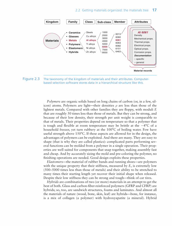
Figure 2.3 illustrates how the families are expanded to show classes, sub-classes and members, each of which is characterized by a set of attributes: itsproperties. As an example, the Materials universe contains the family ‘Metals’,which in turn contains the class ‘Aluminum alloys’, sub-classes such as the‘6000 series’ within which we find the particular member ‘Alloy 6061’. It, andevery other member of the universe, is characterized by a set of attributes thatinclude not only the properties mentioned in Chapter 1, but also its processingcharacteristics, the environmental consequences of its use and its typical appli-cations. We call this its property profile. Selection involves seeking the best matchbetween the property profiles of the materials in the universe and that requiredby the design. As already mentioned, the members of one family have certaincharacteristics in common. Here, briefly, are some of these.
Metals have relatively high stiffness, measured by the modulus, E. Most, whenpure, are soft and easily deformed, meaning that σy is low. They can be madestrong by alloying and by mechanical and heat treatment, increasing σy, butthey remain ductile, allowing them to be formed by deformation processes. And,broadly speaking, they are tough, with a usefully high fracture toughness K1c.They are good electrical and thermal conductors. But metals have weaknessestoo: they are reactive; most corrode rapidly if not protected.
Ceramics are non-metallic, inorganic solids, like porcelain or alumina—thematerial of spark-plug insulators. They have many attractive features. They arestiff, hard and abrasion resistant, they retain their strength to high temperatures,
SteelsCast ironsAl alloys
Cu alloysZn alloysTi alloys
Metals
Elastomers
AluminasSilicon carbides
Silicon nitridesZirconias
Ceramics CompositesSandwiches
Segmented structuresLattices and
foams
Hybrids
PE, PP, PET,PC, PS, PEEK
PA (nylons)
PolyestersPhenolicsEpoxies
Polymers
Soda glassBorosilicate glass
Silica glassGlass-ceramics
Glasses
IsopreneNeoprene
Butyl rubber
Natural rubberSilicones
EVA
Figure 2.1 The menu of engineering materials. The basic families of metals, ceramics,glasses, polymers and elastomers can be combined in various geometries tocreate hybrids.
Ch02-H8391.qxd 1/16/07 5:44 PM Page 15

and they resist corrosion well. Most are good electrical insulators. They, too,have their weaknesses: unlike metals, they are brittle, with low K1c. This givesceramics a low tolerance for stress concentrations (like holes or cracks) or forhigh contact stresses (at clamping points, for instance). For this reason it ismore difficult to design with ceramics than with metals.
Glasses are non-crystalline (‘amorphous’) solids, a term explained more fullyin Chapter 4. The commonest are the soda-lime and borosilicate glasses famil-iar as bottles and Pyrex ovenware, but there are many more. The lack of crys-tal structure suppresses plasticity, so, like ceramics, glasses are hard andremarkably corrosion resistant. They are excellent electrical insulators and, ofcourse, they are transparent to light. But like ceramics, they are brittle and vulnerable to stress concentrations.
16 Chapter 2 Family trees: organizing materials and processes
Elastomers
Polymers
Metals
Hybrids
Glasses
Ceramics
Figure 2.2 Examples of each material family. The arrangement follows the general patternof Figure 2.1. The central hybrid here is a sandwich structure made bycombining stiff, strong face sheets of aluminum with a low-density core ofbalsa wood.
Ch02-H8391.qxd 1/16/07 5:44 PM Page 16
Polymers are organic solids based on long chains of carbon (or, in a few, sil-icon) atoms. Polymers are light—their densities ρ are less than those of thelightest metals. Compared with other families they are floppy, with moduli Ethat are roughly 50 times less than those of metals. But they can be strong, andbecause of their low density, their strength per unit weight is comparable tothat of metals. Their properties depend on temperature so that a polymer thatis tough and flexible at room temperature may be brittle at the 4°C of ahousehold freezer, yet turn rubbery at the 100°C of boiling water. Few haveuseful strength above 150°C. If these aspects are allowed for in the design, theadvantages of polymers can be exploited. And there are many. They are easy toshape (that is why they are called plastics): complicated parts performing sev-eral functions can be molded from a polymer in a single operation. Their prop-erties are well suited for components that snap together, making assembly fastand cheap. And by accurately sizing the mold and pre-coloring the polymer, nofinishing operations are needed. Good design exploits these properties.
Elastomers—the material of rubber bands and running shoes—are polymerswith the unique property that their stiffness, measured by E, is extremely low(500–5000 times less than those of metals) and their ability to be stretched tomany times their starting length yet recover their initial shape when released.Despite their low stiffness they can be strong and tough—think of car tires.
Hybrids are combinations of two (or more) materials in an attempt to get thebest of both. Glass and carbon-fiber-reinforced polymers (GFRP and CFRP) arehybrids; so, too, are sandwich structures, foams and laminates. And almost allthe materials of nature (wood, bone, skin, leaf) are hybrids—bone, for instance,is a mix of collagen (a polymer) with hydroxyapatite (a mineral). Hybrid
2.2 Getting materials organized: the materials tree 17
Materials
•
•
•
•
•
•
Ceramics
Glasses
Metals
Polymers
Elastomers
Hybrids
Steels
Cu alloys
Al alloys
Ti alloys
Ni alloys
Zn alloys
10002000300040005000600070008000
Material records
Density
Mechanical props.
Thermal props.
Electrical props.
Optical props.
Corrosion props.
-- specific
-- general
6013606060616063608261516463
Family Class Member AttributesSub-classKingdom
Density
Mechanical props.
Thermal props.
Electrical props.
Optical props.
Corrosion props.
Documentation
– specific
– general
Al 6061
Figure 2.3 The taxonomy of the kingdom of materials and their attributes. Computer-based selection software stores data in a hierarchical structure like this.
Ch02-H8391.qxd 1/16/07 5:44 PM Page 17

components are expensive and they are relatively difficult to form and join. Sodespite their attractive properties the designer will use them only when theadded performance justifies the added cost. Today’s growing emphasis on highperformance and fuel efficiency provides increasing drivers for their use.
2.3 Organizing processes: the process tree
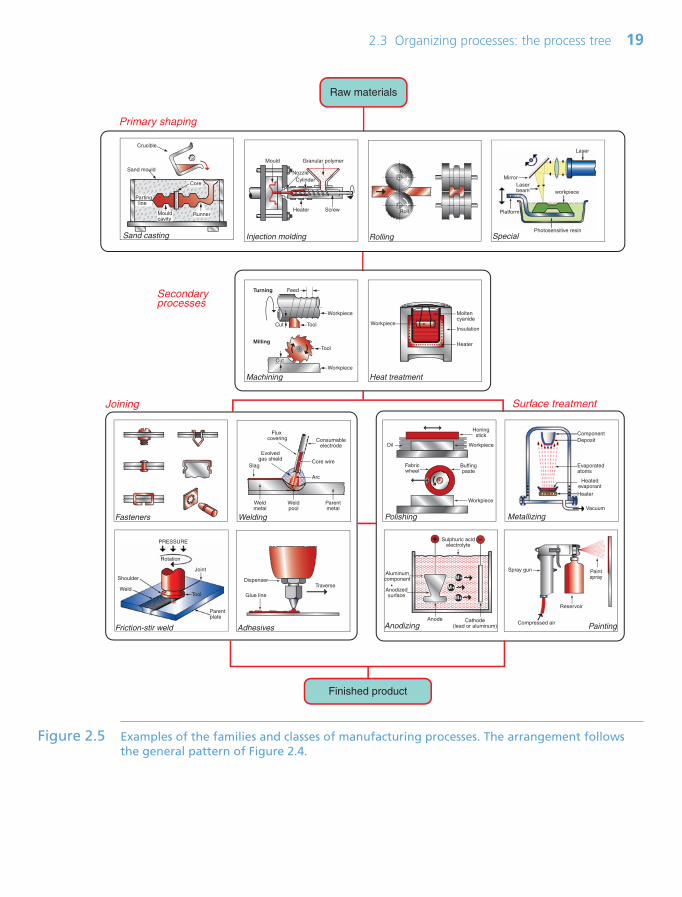
A process is a method of shaping, joining or finishing a material. Casting, injec-tion molding, fusion welding and electro-polishing are all processes; there arehundreds of them (Figures 2.4 and 2.5). It is important to choose the rightprocess-route at an early stage in the design before the cost-penalty of makingchanges becomes large. The choice, for a given component, depends on thematerial of which it is to be made, on its shape, dimensions and precision, andon how many are to be made—in short, on the design requirements.
18 Chapter 2 Family trees: organizing materials and processes
Raw materials
Castingmethods:
SandDie
Investment
Machining:Cut, turn, plane
drill, grind
Heat treat:Quench, temper,
age-harden
Moldingmethods:
InjectionCompressionBlow molding
Deformationmethods:
RollingForgingDrawing
Powdermethods:
SinteringHIPing
Slip casting
Specialmethods:
Rapid prototypeLay-up
Electro-form
Polishing,
Texturing
Plating,
Metallizing
Anodize,
Chromizing
Painting,
Printing
Fastening,
Riveting
Welding,
Heat bonding
Snap fits,
Friction bond
Adhesives,
Cements
Primary shaping
Secondary processes
Surface treatmentJoining
Finished product
Compositeforming:
Hand lay-upFilament winding
RTM
Figure 2.4 The classes of process. The first row contains the primary shaping processes;below lie the secondary processes of machining and heat treatment, followedby the families of joining and finishing processes.
Ch02-H8391.qxd 1/16/07 5:44 PM Page 18
2.3 Organizing processes: the process tree 19
Glue line
DispenserTraverse
Workpiece
Fabricwheel
Buffingpaste
Honingstick
Oil
Workpiece
M+
M+
M+Anodizedsurface
Sulphuric acidelectrolyte
Anode Cathode(lead or aluminum)
Aluminumcomponent
Reservoir
Spray gun
Compressed air
Paintspray
Weldmetal
Consumableelectrode
Flux covering
Core wire
Arc
Slag
Weldpool
Parentmetal
Evolvedgas shield
Vacuum
ComponentDeposit
Evaporatedatoms
HeatedevaporantHeater
Parentplate
Joint
PRESSURE
Shoulder
WeldTool
Rotation
Cut
Turning
Milling
Workpiece
Feed
Cut Tool
Tool
Workpiece
Moltencyanide
Insulation
Heater
Workpiece
Mouldcavity
Runner
Sand mould
Parting line
Core
Crucible
Heater Screw
Granular polymerMould
NozzleCylinder
Roll
Roll
Laser
workpieceLaser beam
Mirror
Platform
Photosensitive resin
Finished product
Raw materials
Primary shaping
Secondaryprocesses
Joining Surface treatment
Sand casting Injection molding Rolling Special
Heat treatmentMachining
Fasteners
Friction-stir weld
Welding
Adhesives
Polishing Metallizing
PaintingAnodizing
Figure 2.5 Examples of the families and classes of manufacturing processes. The arrangement followsthe general pattern of Figure 2.4.
Ch02-H8391.qxd 1/16/07 5:44 PM Page 19

The choice of material limits the choice of process. Polymers can be molded,other materials cannot. Ductile materials can be forged, rolled and drawn butthose that are brittle must be shaped in other ways. Materials that melt at mod-est temperatures to low-viscosity liquids can be cast; those that do not have tobe processed by other routes. Shape, too, influences the choice of process.Slender shapes can be made easily by rolling or drawing but not by casting.Hollow shapes cannot be made by forging, but they can by casting or molding.
Classifying processesManufacturing processes are organized under the headings shown in Figure 2.4.Primary processes create shapes. The first row lists six primary forming processes:casting, molding, deformation, powder methods, methods for forming com-posites, special methods including rapid prototyping. Secondary processesmodify shapes or properties; here they are shown as ‘machining’, which addsfeatures to an already shaped body, and ‘heat treatment’, which enhances sur-face or bulk properties. Below these come joining and, finally, surface treat-ment. Figure 2.5 illustrates some of these; it is organized in the same way asFigure 2.4. The merit of Figure 2.4 is as a flow chart: a progression through amanufacturing route. It should not be treated too literally: the order of thesteps can be varied to suit the needs of the design. The point it makes is thatthere are three broad process families: those of shaping, joining and finishing.
To organize information about processes, we need a hierarchical classifica-tion like that used for materials, giving each process a place. Figure 2.6 showspart of the hierarchy. The Process universe has three families: shaping, joiningand surface treatment. In this figure, the shaping family is expanded to showclasses: casting, deformation, molding etc. One of these—molding—is againexpanded to show its members: rotation molding, blow molding, injectionmolding and so forth. Each process is characterized by a set of attributes: thematerials it can handle, the shapes it can make, their size, precision and an eco-nomic batch size (the number of units that it can make most economically).
The other two families are partly expanded in Figure 2.7. There are threebroad classes of joining process: adhesives, welding and fasteners. In this figureone of them—welding—is expanded to show its members. As before eachmember has attributes. The first is the material or materials that the process canjoin. After that the attribute list differs from that for shaping. Here the geome-try of the joint and the way it will be loaded are important, as are requirementsthat the joint can or cannot be disassembled, be watertight and be electricallyconducting.
The lower part of the figure expands the family of finishing processes. Someof the classes it contains are shown; one—coating—is expanded to show someof its members. Finishing adds cost: the only justification for applying a finish-ing process is that it hardens, or protects, or decorates the surface in ways thatadd value. As with joining, the material to be coated is an important attributebut the others again differ.
We return to process selection in Chapters 18 and 19.
20 Chapter 2 Family trees: organizing materials and processes
Ch02-H8391.qxd 1/16/07 5:44 PM Page 20

2.4 Process–property interaction
Processing can change properties. If you hammer a metal (‘forging’) it get harder;if you then heat it up it gets softer again (‘annealing’). If polyethylene—the stuff
2.4 Process–property interaction 21
Process
Joining
Shaping
Surfacetreatment
Casting
Deformation
Molding
Composite
Powder
Prototyping
CompressionRotationTransferInjectionFoamExtrusionResin casting
Blow moldingThermo-forming
A process record
Material
Shape
Size range
Minimum section
Tolerance
Roughness
Documentation
Family Class Member AttributesKingdom
Minimum batch sizeCost model
Figure 2.6 The taxonomy of the kingdom of process with part of the shaping familyexpanded. Each member is characterized by a set of attributes. Processselection involves matching these to the requirements of the design.
Process records
Heat treat
Paint/print
Coat
Polish
Texture ...
Electroplate
Anodize
Powder coat
Metallize...
Material
Purpose of treatment
Coating thickness
Surface hardness
Relative cost ...
Supporting information
Material
Purpose of treatment
Coating thickness
Surface hardness
Relative cost ...
Documentation
Adhesives
Welding
Fasteners
Braze
GasArc
e-beam Hot gas
Material
Joint geometry
Size Range
Section thickness
Relative cost ...
Supporting information
Material
Joint geometry
Size range
Section thickness
Relative cost ...
Documentation
Class AttributesMemberKingdom
Surfacetreatment
Joining
Family
ShapingProcess
Solder
Hot bar...
Figure 2.7 The taxonomy of the process kingdom again, with the families of joining andfinishing partly expanded.
Ch02-H8391.qxd 1/16/07 5:44 PM Page 21

of plastic bags—is drawn to a fiber, its strength is increased by a factor of 5.Soft, stretchy rubber is made hard and brittle by vulcanizing. Heat-treatingglass in a particular way can give it enough impact resistance to withstand aprojectile (‘bullet-proof glass’). And composites like carbon-fiber-reinforcedepoxy have no useful properties at all until processed—prior to processing theyare just a soup of resin and a sheaf of fibers.
Joining, too, changes properties. Welding involves the local melting and re-solidifying of the faces of the parts to be joined. As you might expect, the weldzone has properties that differ from those of the material far from the weld—usuallyworse. Surface treatments, by contrast, are generally chosen to improve properties:electroplating to improve corrosion resistance, carburizing to improve wear.
Process–property interaction appears in a number of chapters. We return toit specifically in Chapter 19.
2.5 Material property charts
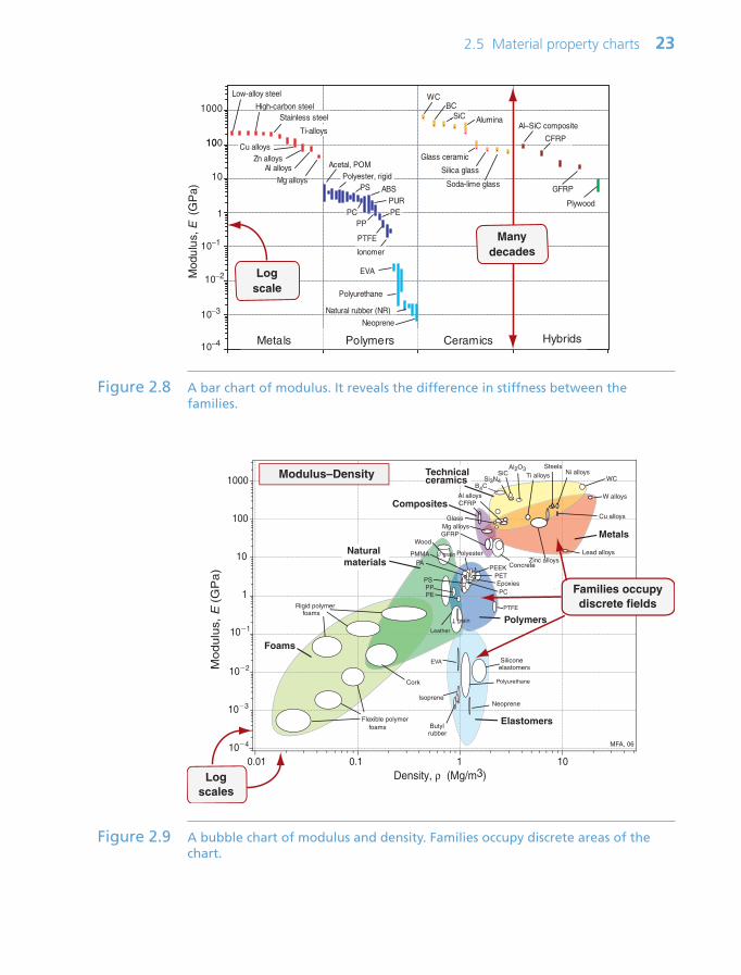
Data sheets for materials list their properties; they give no perspective and pres-ent no comparisons. The way to achieve these is to plot material propertycharts. They are of two types: bar charts and bubble charts.
A bar chart is simply a plot of one property for all the materials of the uni-verse. Figure 2.8 shows an example: it is a bar chart for modulus, E. The largestis more than 10 million times greater than the smallest—many other propertieshave similar ranges—so it makes sense to plot them on logarithmic1, not linearscales, as here. The length of each bar shows the range of the property for eachmaterial, here segregated by family. The differences between the families nowbecome apparent. Metals and ceramics have high moduli. Those of polymersare smaller, by a factor of about 50, than those of metals; those of elastomersare some 500 times smaller still.
More information is packed into the picture if two properties are plotted to givea bubble chart, as in Figure 2.9, here showing modulus E and density ρ. As before,the scales are logarithmic. Now families are more distinctly separated: all metalslie in the reddish zone near the top right; all polymers lie in the dark blue enve-lope in the center, elastomers in the lighter blue envelope below, ceramics in theyellow envelope at the top. Each family occupies a distinct, characteristic field.
Material property charts like these are a core tool, used throughout this book.
• They give an overview of the physical, mechanical and functional propertiesof materials, presenting the information about them in a compact way.
• They reveal aspects of the physical origins of properties, helpful in under-standing the underlying science.
• They become a tool for optimized selection of materials to meet given designrequirements, and they help understand the use of materials in existing products.
22 Chapter 2 Family trees: organizing materials and processes
1Logarithmic means that the scale goes up in constant multiples, usually of 10. We live in alogarithmic world—our senses, for instance, all respond in that way.
Ch02-H8391.qxd 1/16/07 5:44 PM Page 22
2.5 Material property charts 23
10
100
1000
Low alloy steel
Mg alloys
Al alloysZn-alloys
Cu-alloys
Stainless steelHigh-carbon steel
Acetal, POM
Polyurethane
EVA
IonomerPTFE
WC
Alumina
Glass Ceramic
Silica glass
Soda-Lime glassPolyester, rigid
PC
PS
PURPE
ABS
PP
BCSiC
Al-SiC Composite
CFRP
GFRP
Plywood
Natural Rubber (NR)
CompositesPolymersMetals Ceramics & glassMetals Polymers Ceramics Hybrids
10
Low-alloy steel
Zn alloysCu-alloys
Acetal, POM
EVA
IonomerPTFE
WC
Alumina
Glass ceramic
Soda-lime glassPolyester, rigid
PC
PS
PURPE
ABS
PP
BCSiC
Al-SiC Composite
CFRP
Neoprene
Natural rubber (NR)
CompositesPolymersMetals Ceramics & glass
Cu alloys
Acetal, POM
EVA
Ionomer
PTFE
Alumina
Polyester, rigidPS
PURPE
ABS
PP
SiCAl–SiC composite
CompositesPolymersMetals Ceramics & glass
1
10−1
Acetal, POM
EVA
PTFE
Polyester, rigid
PP
CompositesPolymersMetals Ceramics & glass
Mod
ulu
s, E
(G
Pa)
Metals Polymers Ceramics Hybrids
10−2
10−3
10−4
Stainless steel
Ti-alloys
Logscale
Manydecades
Figure 2.8 A bar chart of modulus. It reveals the difference in stiffness between thefamilies.
Density, ρ (Mg/m3)0.01
Mo
du
lus,
E (
GP
a)
104
0.1 1 10
103
102
101
1
10
100
1000
Polyester
Foams
Polymers
Metals
Technicalceramics
Composites
Lead alloys
W alloys
SteelsTi alloys
Mg alloys
CFRP
GFRP
Al alloys
Rigid polymer foams
Flexible polymer foams
Ni alloys
Cu alloys
Zinc alloysPAPEEK
PMMA
PC
PET
Cork
Wood
Butyl rubber
Silicone elastomers
Concrete
WC
Al2O3SiC
Si3N4Modulus–Density
B4C
EpoxiesPS
PTFE
EVA
NeopreneIsoprene
Polyurethane
Leather
MFA, 06
PPPE
Glass
// grain
grainT
Elastomers
Natural materials
Families occupydiscrete fields
Logscales
Figure 2.9 A bubble chart of modulus and density. Families occupy discrete areas of thechart.
Ch02-H8391.qxd 1/16/07 5:44 PM Page 23
These two charts, and all the others in the book, were made using the CESsoftware, which allows charts of any pair of properties, or of functions of prop-erties (like E/ρ) to be created at will. Their uses, and the operations they allow,will emerge in the chapters that follow.
2.6 Computer-aided information management for materials and processes
Classification is the first step in creating an information management systemfor materials and processes. In it records for the members of each universe areindexed, so to speak, by their position in the tree-like hierarchies of Figures 2.3,2.6 and 2.7. Each record has a unique place, making retrieval easy.
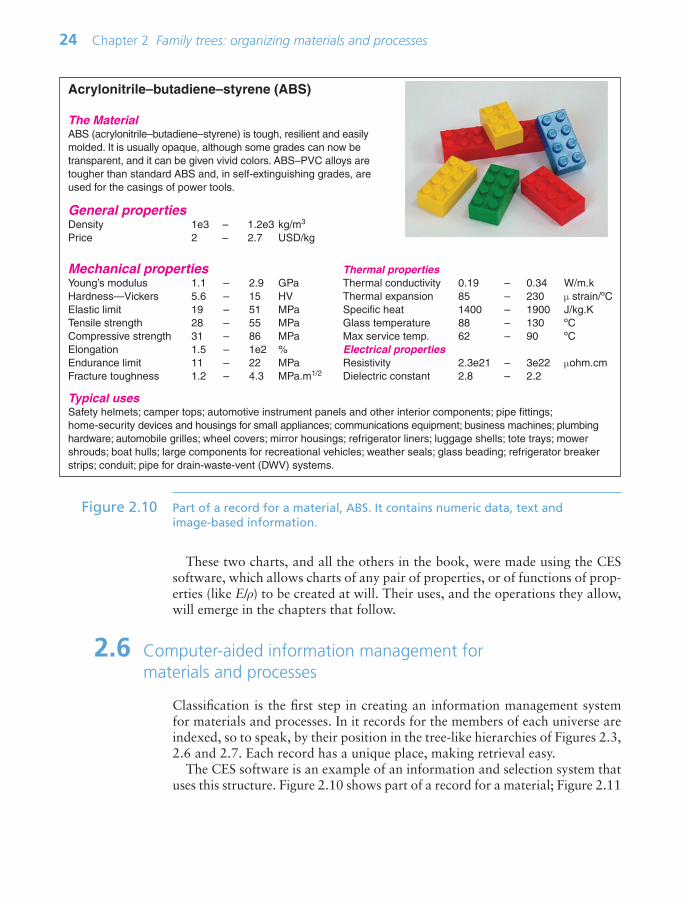
The CES software is an example of an information and selection system thatuses this structure. Figure 2.10 shows part of a record for a material; Figure 2.11
24 Chapter 2 Family trees: organizing materials and processes
Acrylonitrile–butadiene–styrene (ABS)
The MaterialABS (acrylonitrile–butadiene–styrene) is tough, resilient and easilymolded. It is usually opaque, although some grades can now betransparent, and it can be given vivid colors. ABS–PVC alloys aretougher than standard ABS and, in self-extinguishing grades, areused for the casings of power tools.
General propertiesDensity 1e3 – 1.2e3 kg/m3
Price 2 – 2.7 USD/kg
Mechanical properties Thermal propertiesYoung’s modulus 1.1 – 2.9 GPa Thermal conductivity 0.19 – 0.34 W/m.kHardness—Vickers 5.6 – 15 HV Thermal expansion 85 – 230 µ strain/ºCElastic limit 19 – 51 MPa Specific heat 1400 – 1900 J/kg.KTensile strength 28 – 55 MPa Glass temperature 88 – 130 ºCCompressive strength 31 – 86 MPa Max service temp. 62 – 90 ºCElongation 1.5 – 1e2 % Electrical propertiesEndurance limit 11 – 22 MPa Resistivity 2.3e21 – 3e22 µohm.cmFracture toughness 1.2 – 4.3 MPa.m1/2 Dielectric constant 2.8 – 2.2
Typical usesSafety helmets; camper tops; automotive instrument panels and other interior components; pipe fittings;home-security devices and housings for small appliances; communications equipment; business machines; plumbinghardware; automobile grilles; wheel covers; mirror housings; refrigerator liners; luggage shells; tote trays; mowershrouds; boat hulls; large components for recreational vehicles; weather seals; glass beading; refrigerator breakerstrips; conduit; pipe for drain-waste-vent (DWV) systems.
Figure 2.10 Part of a record for a material, ABS. It contains numeric data, text andimage-based information.
Ch02-H8391.qxd 1/16/07 5:44 PM Page 24
shows the same for a process. A record is found by opening the tree,following the branches until the desired record is located (‘browsing’) or bylocating it by name using a text-search facility (‘searching’).
Don’t worry for the moment about the detailed content of the records—theyare explained in later chapters. Note only that each contains data of two types.Structured data are numeric, Boolean (Yes/No) or discrete (e.g. Low / Medium /High), and can be stored in tables. Later chapters show how structured data areused for selection. Unstructured data take the form of text, images, graphs andschematics. Such information cannot so easily be used for selection but it isessential for the step we refer to in the next chapter as ‘documentation’.
2.7 Summary and conclusions
There are six broad families of materials for design: metals, ceramics, glasses,polymers, elastomers and hybrids that combine the properties of two or more ofthe others. Processes, similarly, can be grouped into families: those that createshape, those that join and those that modify the surface to enhance its properties
2.7 Summary and conclusions 25
Injection molding
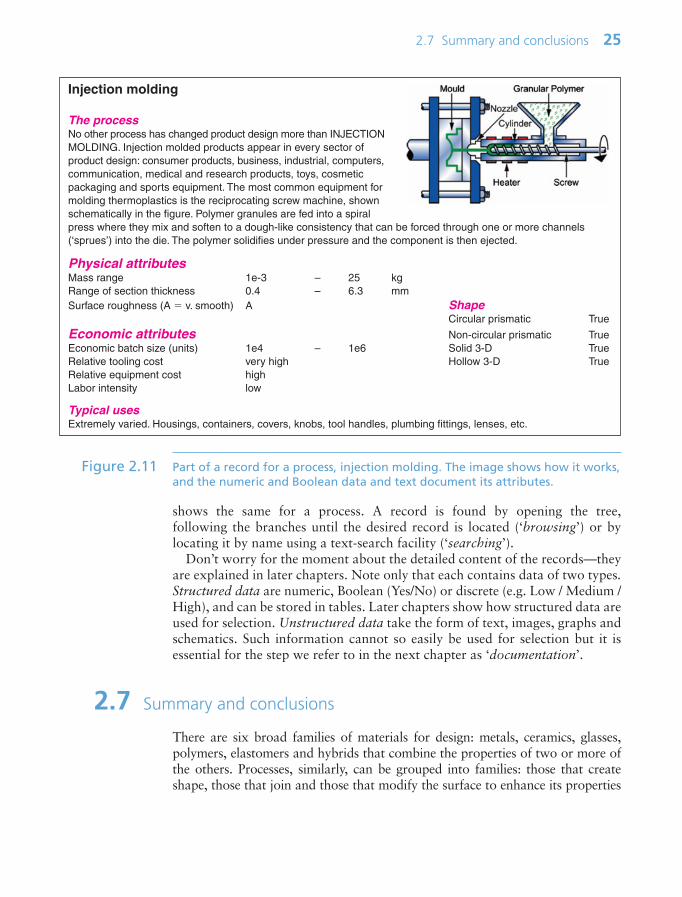
The processNo other process has changed product design more than INJECTIONMOLDING. Injection molded products appear in every sector ofproduct design: consumer products, business, industrial, computers,communication, medical and research products, toys, cosmeticpackaging and sports equipment. The most common equipment formolding thermoplastics is the reciprocating screw machine, shownschematically in the figure. Polymer granules are fed into a spiralpress where they mix and soften to a dough-like consistency that can be forced through one or more channels(‘sprues’) into the die. The polymer solidifies under pressure and the component is then ejected.
Physical attributesMass range 1e-3 – 25 kgRange of section thickness 0.4 – 6.3 mmSurface roughness (A v. smooth) A Shape
Circular prismatic True
Economic attributes Non-circular prismatic TrueEconomic batch size (units) 1e4 – 1e6 Solid 3-D TrueRelative tooling cost very high Hollow 3-D TrueRelative equipment cost highLabor intensity low
Typical usesExtremely varied. Housings, containers, covers, knobs, tool handles, plumbing fittings, lenses, etc.
Figure 2.11 Part of a record for a process, injection molding. The image shows how it works,and the numeric and Boolean data and text document its attributes.
Ch02-H8391.qxd 1/16/07 5:44 PM Page 25
or to protect or decorate it. The members of the families can be organized into ahierarchical tree-like catalog, allowing them to be ‘looked up’ in much the sameway that you would look up a member of a company in the companies manage-ment sheet. A record for a member stores information about it: numeric and othertabular data for its properties, text, graphs and images to describe its use andapplications. This structure forms the basis of computer-based selection systems ofwhich the CES system is an example. It enables a unique way of presenting datafor materials and processes as property charts, two of which appear in this chapter.They become one of the central features of the chapters that follow.
2.8 Further reading
Ashby, M.F. and Johnson, K. (2002) Materials and Design—The Art and Science ofMaterial Selection in Product Design, Butterworth-Heinemann, Oxford, UK. ISBN0-7506-5554-2. (Materials and processes from an aesthetic point of view, emphasizingproduct design.)
Bralla, J.G. (1998) Design for Manufacturability Handbook, 2nd edition, McGraw-Hill, New York, USA. ISBN 0-07-007139-X. (Turgid reading, but a rich mine ofinformation about manufacturing processes.)
Callister, W.D. (2003) Materials Science and Engineering, An Introduction, 6th edition,John Wiley, New York, USA. ISBN 0-471-13576-3. (A well-respected materials text,now in its 6th edition, widely used for materials teaching in North America.)
Charles, J.A., Crane, F.A.A. and Furness, J.A.G. (1997) Selection and Use ofEngineering Materials, 3rd edition, Butterworth-Heinemann, Oxford, UK. ISBN0-7506-3277-1. (A Materials Science approach to the selection of materials.)
Dieter, G.E. (1991) Engineering Design, A Materials and Processing Approach, 2nd edi-tion, McGraw-Hill, New York, USA. ISBN 0-07-100829-2. (A well-balanced andrespected text focusing on the place of materials and processing in technical design.)
Farag, M.M. (1989) Selection of Materials and Manufacturing Processes forEngineering Design, Prentice-Hall, Englewood Cliffs, NJ, USA. ISBN 0-13-575192-6.(A Materials Science approach to the selection of materials.)
Kalpakjian, S. and Schmid, S.R. (2003) Manufacturing Processes for EngineeringMaterials, 4th edition, Prentice-Hall, Pearson Education, New Jersey, USA. ISBN0-13-040871-9. (A comprehensive and widely used text on material processing.)
26 Chapter 2 Family trees: organizing materials and processes
2.9 Exercises
Exercise E2.1 List the six main classes of engineering materials. Use your own experienceto rank them approximately:`(a) By stiffness (modulus, E).(b) By thermal conductivity (λ).
Ch02-H8391.qxd 1/16/07 5:44 PM Page 26
2.9 Exercises 27
Exercise E2.2 Examine the material property chart of Figure 2.9. By what factor are polymersless stiff than metals? Is wood denser or less dense than polyethylene (PE)?
Exercise E2.3 What is meant by a shaping process? Look around you and ask yourself howthe things you see were shaped.
Exercise E2.4 Almost all products involve several parts that are joined. Examine the prod-ucts immediately around you and list the joining methods used to assemblethem.
Exercise E2.5 How many different surface treatment processes can you think of, based onyour own experience? List them and annotate the list with the materials towhich they are typically applied.
Exercise E2.6 How many ways can you think of for joining two sheets of a plastic likepolyethylene? List each with an example of an application that might use it.
Exercise E2.7 A good classification looks simple—think, for instance, of the Periodic Tableof the elements. Creating it in the first place, however, is another matter. Thischapter introduced two classification schemes that work, meaning that everymember of the scheme has a unique place in it, and any new member can beinserted into its proper position without disrupting the whole. Try one foryourself. Here are some scenarios. Make sure that each level of the hierarchyproperly contains all those below it. There may be more than one way to dothis, but one is usually better than the others. Test it by thinking how youwould use it to find the information you want.(a) You run a bike shop that stocks bikes of many types, prices and sizes.
You need a classification system to allow customers to look up yourbikes on the internet. How would you do it?
(b) You are asked to organize the inventory of fasteners in your company.There are several types (snap, screw, rivet) and, within each, a range ofmaterials and sizes. Devise a classification scheme to store informationabout them.
Ch02-H8391.qxd 1/16/07 5:44 PM Page 27
28 Chapter 2 Family trees: organizing materials and processes
2.10 Exploring design using CES
Designers need to be able to find data quickly and reliably. That is where the clas-sifications come in. The CES system uses the classification scheme described inthis chapter. Before trying these exercises, open the Materials Universe in CES andexplore it. The opening screen offers options—take the Edu Level 1: Materials.
Exercise E2.8 Use the ‘Browse’ facility in Level 1 of the CES Software to find the record forCopper. What is its thermal conductivity? What is its price?
Exercise E2.9 Use the ‘Browse’ facility in Level 1 of the CES Software to find the record forthe thermosetting polymer Phenolic. Are they cheaper or more expensivethan Epoxies?
Exercise E2.10 Use the ‘Browse’ facility to find records for the polymer-shaping processesRotational molding. What, typically, is it used to make?
Exercise E2.11 Use the ‘Search’ facility to find out what Plexiglas is. Do the same for Pyroceram.
Exercise E2.12 Use the ‘Search’ facility to find out about the process Pultrusion. Do the samefor TIG welding. Remember that you need to search the Process Universe,not the Material Universe.
Exercise E2.13 Compare Young’s modulus E (the stiffness property) and thermal conductiv-ity λ (the heat transmission property) of aluminum alloys (a non-ferrousmetal), alumina (a technical ceramic), polyethylene (a thermoplastic polymer)and neoprene (an elastomer) by retrieving values from CES Level 1. Which has thehighest modulus? Which has the lowest thermal conductivity?
2.11 Exploring the science with CES Elements
The CES system contains a database for the Periodic Table. The records con-tain fundamental data for each of the elements. We will use this in the book todelve a little deeper into the science that lies behind material properties.
Exercise E2.14 Refresh your memory of the Periodic Table, perhaps the most significant classi-fication of all time. Select CES Elements (File Change database CESElements) and double-click on Periodic Table to see the table. This database,like the others described in this chapter, has a tree-like structure. Use this to findthe record for Aluminum (Row 3, Atomic number 13) and explore its contents.Many of the properties won’t make sense yet. We introduce them graduallythroughout the book.
Ch02-H8391.qxd 1/16/07 5:44 PM Page 28

Chapter 3Strategic thinking: matching
material to design
Images embodying the concepts described in the text:pull, geared pull, shear and pressure. (Image courtesy
of A-Best Fixture Co. 424 West Exchange Street,Akron, Ohio, 44302, USA.)
Chapter contents
3.1 Introduction and synopsis 303.2 The design process 303.3 Material and process information
for design 343.4 The strategy: translation, screening,
ranking and documentation 363.5 Examples of translation 393.6 Summary and conclusions 433.7 Further reading 433.8 Exercises 443.9 Exploring design using CES 46
Ch03-H8391.qxd 1/17/07 11:38 AM Page 29

30 Chapter 3 Strategic thinking: matching material to design
3.1 Introduction and synopsis
Our aim in this chapter is to develop a strategy for selecting materials andprocesses that is design-led; that is, the strategy uses, as inputs, the require-ments of the design. To do so we must first look briefly at design itself. Thischapter introduces some of the words and phrases—the vocabulary—of design,the stages in its implementation and the ways in which materials selection linkswith these.
Design starts with a market need. The need is analyzed, expressing it as a setof design requirements. Ways to meet these (‘concepts’) are sought, developed(‘embodied’) and refined (‘detailed’) to give a product specification. The choiceof material and process evolves in parallel with this process, in the way detailedin this chapter.
With this background we can develop the selection strategy. It involves foursteps: translation, screening, ranking and documentation. These steps areexplained and the first, that of translation, is illustrated with examples.
3.2 The design process
Original design starts from a new concept and develops the information neces-sary to implement it. Evolutionary design (or redesign) starts with an existingproduct and seeks to change it in ways that increase its performance, reduce itscost, or both.
Original designOriginal design starts from scratch. It involves a new idea or working principle(the audio tape, the compact disc and the MP3 player were all, in their day,completely new). Original design can be stimulated by new materials. Thus, high-purity silicon enabled the transistor; high-purity glass, the optical fiber; highcoercive-force magnets, the miniature earphone; solid-state lasers, the compactdisc. Sometimes the new material suggests the new product. Sometimes insteadthe new product demands the development of a new material: nuclear technologydrove the development of new zirconium alloys and new stainless steels; spacetechnology stimulated the development of beryllium alloys and lightweightcomposites; turbine technology today drives development of high-temperaturealloys and ceramics.
The central column of Figure 3.1 shows the design process. The starting pointis a market need or a new idea; the end point is the full product specificationfor a product that fills the need or embodies the idea. A need must be identifiedbefore it can be met. It is essential to define the need precisely—that is, to formu-late a need statement, often in the form: ‘a device is required to perform task X’,expressed as a set of design requirements. Between the need statement and theproduct specification lie the set of stages shown in Figure 3.1: the stages of con-ceptual design, embodiment design and detailed design, explained in a moment.
Ch03-H8391.qxd 1/17/07 11:38 AM Page 30

3.2 The design process 31
At the conceptual design stage, all options are open: the designer considersalternative concepts and the ways in which these might be separated or com-bined. The next stage, embodiment, takes the promising concepts and seeks toanalyze their operation at an approximate level. This involves sizing the com-ponents and a preliminary selection of materials and processes, examining theimplications for performance and cost. The embodiment stage ends with a feas-ible layout, which becomes the input to the detailed design stage. Here specifi-cations and dimensions for each component are drawn up. Critical componentsmay be subjected to precise mechanical or thermal analysis. Optimization meth-ods are applied to components and groups of components to maximize perfor-mance, minimize cost and ensure safety. A final choice of geometry and materialis made, and the methods of production are analyzed and costed. The stageends with a detailed product specification.
RedesignMost design is not ‘original’ in the sense of starting from a totally new idea. Itis redesign, starting with an existing product and correcting its shortcomings,refining it, enhancing its performance or reducing its cost, without discardingthe principles on which it operates or—frequently—many of its components.
Market need:problem definition
Productspecification
Conceptexplore working
principles
Embodimentdefine general
layout and scale
Detailoptimize form,
manufacture and assembly
Choice of material family
(metals, ceramics... )
Choice of materialclass
(steel, Al alloy, Nl alloy)
Material data needs
Choice of singlematerial
(6061 Al; 304 stainless)
Choice of processfamily
(casting, molding... )
Choice of processclass
(die cast, sand cast... )
Process data needs
Choice of singleprocess
(pressure die cast ... )
Figure 3.1 The design flow chart, showing how material and process selection enter.Information about materials is needed at each stage, but at very different levelsof breadth and precision. The broken lines suggest the iterative nature oforiginal design and the path followed in redesign.
Ch03-H8391.qxd 1/17/07 11:38 AM Page 31

Here are some scenarios that call for redesign. First, the most obvious, the‘product recall’ scenario. If a product, once released to the market, fails to meetsafety standards, urgent redesign is required. Often the problem is a materialfailure; then an alternative must be found that retains the desirable features ofthe original but overcomes its weaknesses. Then there is the ‘poor value formoney’ scenario: the product performs safely but offers performance that, at itsprice, is perceived to be mediocre, requiring redesign to enhance performance.There is, too, the ‘inadequate profit margin’ scenario in which the cost of man-ufacture exceeds the price that the market will bear. Much of the cost of a mass-produced product derives from the materials of which it is made and theprocesses chosen to make it; the response is to re-examine both, with cost-cutting as the objective. Then there is the ‘stay ahead of the competition’ sce-nario. Makers of household products and electronic gadgetry (electric kettles,mobile phones) release new editions annually; those that make cars producenew models every two or three years. In a market environment in which manyalmost identical products compete for the consumers’ attention, it is visual andstylistic character that sets some products above others. Much creative think-ing goes into this ‘industrial design’ and in it the choice of material, or of achange of material, is dictated mainly by aesthetics: color, texture, feel and theability to be shaped or finished in a given way.
Much of redesign has to do with detail—the last of the three boxes in thecentral window of Figure 3.1. But not all. The necessary changes may require achange of configuration and layout—the embodiment phase—or even of basicconcept, replacing one of the ways of performing a function by another. So theflow chart in Figure 3.1 remains a useful summary to keep in mind. It hasanother use, too—as a tool (one of several) for analyzing existing designs andunderstanding how sometimes quirky details of the final product have their ori-gins in decisions made in the concept or embodiment stages.
Described in the abstract, these ideas are not easy to grasp. An example willhelp. Here it is.
Devices to open corked bottlesWhen you buy a bottle of wine you find, generally, that it is sealed with a cork.This creates a market need: it is the need to gain access to the wine inside. Wemight state it thus: ‘A device is required to allow access to wine in a corked bot-tle’ and might add, ‘with convenience, at modest cost, and without contaminat-ing the wine’.
Three concepts for doing this are shown in Figure 3.2. In order, they are: toremove the cork by axial traction (pulling); to remove it by shear tractions; topush it out from below. In the first, a screw is threaded into the cork to whichan axial pull is applied; in the second, slender elastic blades inserted down thesides of the cork apply shear tractions when pulled; and in the third, the corkis pierced by a hollow needle through which a gas is pumped to push it out.
Figure 3.3 shows embodiment sketches for devices based on concept (a), thatof axial traction. The first is a direct pull; the other three use some sort of
32 Chapter 3 Strategic thinking: matching material to design
Ch03-H8391.qxd 1/17/07 11:38 AM Page 32
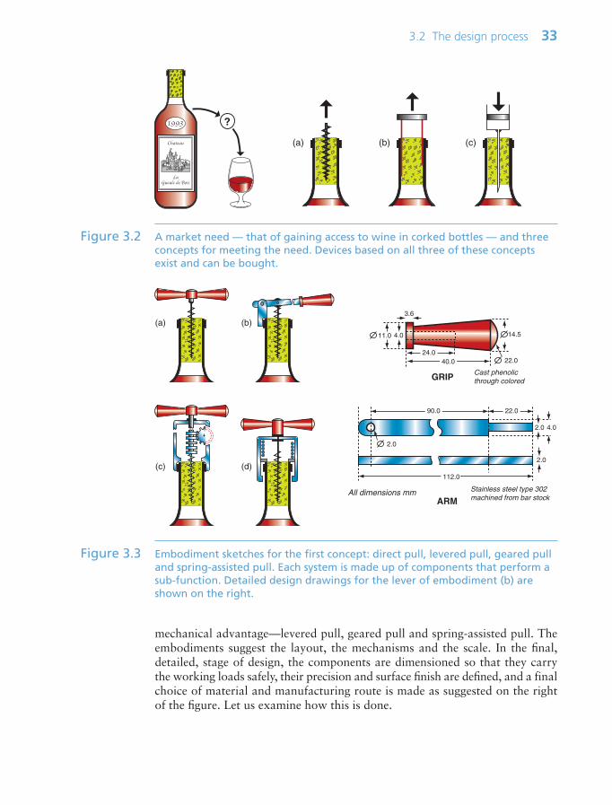
mechanical advantage—levered pull, geared pull and spring-assisted pull. Theembodiments suggest the layout, the mechanisms and the scale. In the final,detailed, stage of design, the components are dimensioned so that they carrythe working loads safely, their precision and surface finish are defined, and a finalchoice of material and manufacturing route is made as suggested on the rightof the figure. Let us examine how this is done.
3.2 The design process 33
?
(a) (b) (c)
Figure 3.2 A market need — that of gaining access to wine in corked bottles — and threeconcepts for meeting the need. Devices based on all three of these conceptsexist and can be bought.
(a) (b)
(c) (d)
4.02.0
2.0
22.0
24.0
90.0
112.0
2.0
Stainless steel type 302machined from bar stockARM
40.0
3.6
4.011.0 14.5
22.0
Cast phenolicthrough coloredGRIP
All dimensions mm
Figure 3.3 Embodiment sketches for the first concept: direct pull, levered pull, geared pulland spring-assisted pull. Each system is made up of components that perform asub-function. Detailed design drawings for the lever of embodiment (b) areshown on the right.
Ch03-H8391.qxd 1/17/07 11:38 AM Page 33
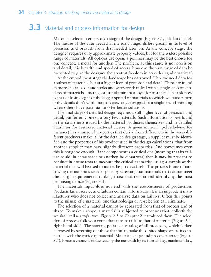
3.3 Material and process information for design
Materials selection enters each stage of the design (Figure 3.1, left-hand side).The nature of the data needed in the early stages differs greatly in its level ofprecision and breadth from that needed later on. At the concept stage, thedesigner requires only approximate property values, but for the widest possiblerange of materials. All options are open: a polymer may be the best choice forone concept, a metal for another. The problem, at this stage, is not precisionand detail, it is breadth and speed of access: how can the vast range of data bepresented to give the designer the greatest freedom in considering alternatives?
At the embodiment stage the landscape has narrowed. Here we need data fora subset of materials, but at a higher level of precision and detail. These are foundin more specialized handbooks and software that deal with a single class or sub-class of materials—metals, or just aluminum alloys, for instance. The risk nowis that of losing sight of the bigger spread of materials to which we must returnif the details don’t work out; it is easy to get trapped in a single line of thinkingwhen others have potential to offer better solutions.
The final stage of detailed design requires a still higher level of precision anddetail, but for only one or a very few materials. Such information is best foundin the data sheets issued by the material producers themselves and in detaileddatabases for restricted material classes. A given material (polyethylene, forinstance) has a range of properties that derive from differences in the ways dif-ferent producers make it. At the detailed design stage, a supplier must be identi-fied and the properties of his product used in the design calculations; that fromanother supplier may have slightly different properties. And sometimes eventhis is not good enough. If the component is a critical one (meaning that its fail-ure could, in some sense or another, be disastrous) then it may be prudent toconduct in-house tests to measure the critical properties, using a sample of thematerial that will be used to make the product itself. The process is one of nar-rowing the materials search space by screening out materials that cannot meetthe design requirements, ranking those that remain and identifying the mostpromising choice (Figure 3.4).
The materials input does not end with the establishment of production.Products fail in service and failures contain information. It is an imprudent man-ufacturer who does not collect and analyze data on failures. Often this pointsto the misuse of a material, one that redesign or re-selection can eliminate.
The selection of a material cannot be separated from that of process and ofshape. To make a shape, a material is subjected to processes that, collectively,we shall call manufacture. Figure 2.5 of Chapter 2 introduced them. The selec-tion of process follows a route that runs parallel to that of material (Figure 3.1,right-hand side). The starting point is a catalog of all processes, which is thennarrowed by screening out those that fail to make the desired shape or are incom-patible with the choice of material. Material, shape and process interact (Figure3.5). Process choice is influenced by the material: by its formability, machinability,
34 Chapter 3 Strategic thinking: matching material to design
Ch03-H8391.qxd 1/17/07 11:38 AM Page 34
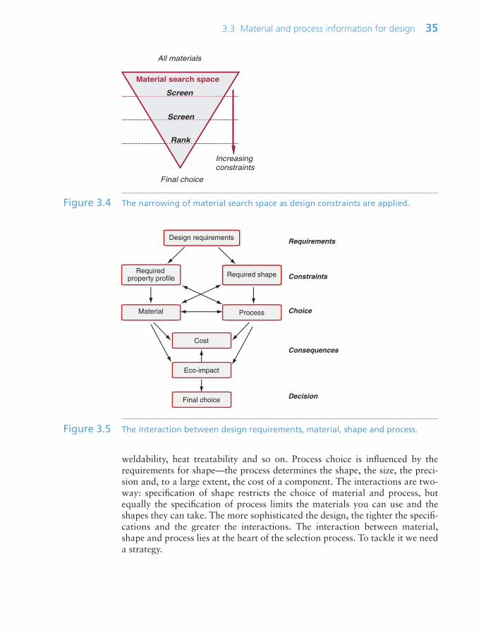
weldability, heat treatability and so on. Process choice is influenced by therequirements for shape—the process determines the shape, the size, the preci-sion and, to a large extent, the cost of a component. The interactions are two-way: specification of shape restricts the choice of material and process, butequally the specification of process limits the materials you can use and theshapes they can take. The more sophisticated the design, the tighter the specifi-cations and the greater the interactions. The interaction between material,shape and process lies at the heart of the selection process. To tackle it we needa strategy.
3.3 Material and process information for design 35
Final choice
Material search space
Screen
Screen
Rank
All materials
Material search space
Screen
Screen
Rank
Material search space
Screen
Screen
Rank
Increasing constraints
Design requirements
Required property profile Required shape
Material Process
Cost
Eco-impact
Final choice
Requirements
Constraints
Choice
Consequences
Decision
Figure 3.4 The narrowing of material search space as design constraints are applied.
Figure 3.5 The interaction between design requirements, material, shape and process.
Ch03-H8391.qxd 1/17/07 11:38 AM Page 35

3.4 The strategy: translation, screening, ranking and documentation
Selection involves seeking the best match between the attribute profiles of the materials and processes—bearing in mind that these must be mutuallycompatible—and those required by the design. The strategy, applied to materi-als, is sketched in Figure 3.6. The first task is that of translation: converting thedesign requirements into a prescription for selecting a material. This proceedsby identifying the constraints that the material must meet and the objectivesthat the design must fulfill. These become the filters: materials that meet theconstraints and rank highly in their ability to fulfill the objectives are potentialcandidates for the design. The second task, then, is that of screening: eliminat-ing the material that cannot meet the constraints. This is followed by the rank-ing step, ordering the survivors by their ability to meet a criterion of excellence,such as that of minimizing cost. The final task is to explore the most promisingcandidates in depth, examining how they are used at present, how best todesign with them, case histories of failures and a step we call documentation.
36 Chapter 3 Strategic thinking: matching material to design
Translate design requirements:express as function, constraints,
objectives and free variables
All materials
Final material choice
Screen using constraints: eliminate materials that
cannot do the job
Rank using objective:find the screened materials
that do the job best
Seek documentation: research the family history of
top-ranked candidates
Figure 3.6 The strategy applied to materials. The same strategy is later adapted to selectprocesses. There are four steps: translation, screening, ranking and supportinginformation. All can be implemented in software, allowing large populations ofmaterials to be investigated.
Ch03-H8391.qxd 1/17/07 11:38 AM Page 36

Process selection follows a parallel route. In this case translation means iden-tifying the geometric and other constraints—dimensions, shape, precision andmaterial compatibility—that must be met, using these to screen out processesthat cannot provide them. We return to process selection in Chapters 18 and19. For now we stick to materials.
TranslationAny engineering component has one or more functions: to support a load, tocontain a pressure, to transmit heat and so forth. This must be achieved subjectto constraints: that certain dimensions are fixed, that the component mustcarry the design loads without failure, the need to insulate against or to con-duct heat or electricity, that it can function in a certain range of temperatureand in a given environment, and many more. In designing the component, thedesigner has one or more objectives: to make it as cheap as possible, perhaps,or as light, or as safe, or some combination of these. Certain parameters can beadjusted in order to optimize the objective—the designer is free to vary dimen-sions that are not constrained by design requirements and, most importantly,free to choose the material for the component and the process to shape it. Werefer to these as free variables.
Constraints, objectives and free variables (Table 3.1) define the boundaryconditions for selecting a material and—in the case of load-bearing components—a shape for its cross-section.
It is important to be clear about the distinction between constraints and objec-tives. A constraint is an essential condition that must be met, usually expressedas a limit on a material or process attribute. An objective is a quantity for whichan extreme value (a maximum or minimum) is sought, frequently cost, mass orvolume, but there are others (Table 3.2). Getting it right can take a little thought.In choosing materials for a super-light sprint bicycle, for example, the objectiveis to minimize mass, with an upper limit on cost, thus treating cost as a constraint.But in choosing materials for a cheap ‘shopping’ bike the two are reversed: nowthe objective is to minimize cost with a (possible) upper limit on mass, thus treat-ing it as a constraint (Figure 3.7).
The outcome of the translation step is a list of the design-limiting propertiesand the constraints they must meet. The first step in relating design requirementsto material properties is therefore a clear statement of function, constraints,objectives and free variables.
3.4 The strategy: translation, screening, ranking and documentation 37
Function • What does the component do?
Constraints • What non-negotiable conditions must be met?
Objective • What is to be maximized or minimized?
Free variables • What parameters of the problem is the designer free to change?
Table 3.1 Function, constraints, objectives and free variables
Ch03-H8391.qxd 1/17/07 11:38 AM Page 37
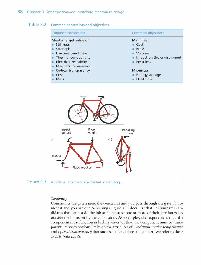
ScreeningConstraints are gates: meet the constraint and you pass through the gate, fail tomeet it and you are out. Screening (Figure 3.6) does just that: it eliminates can-didates that cannot do the job at all because one or more of their attributes liesoutside the limits set by the constraints. As examples, the requirement that ‘thecomponent must function in boiling water’ or that ‘the component must be trans-parent’ imposes obvious limits on the attributes of maximum service temperatureand optical transparency that successful candidates must meet. We refer to theseas attribute limits.
38 Chapter 3 Strategic thinking: matching material to design
Common constraints Common objectives
Meet a target value of Minimize• Stiffness • Cost• Strength • Mass• Fracture toughness • Volume• Thermal conductivity • Impact on the environment• Electrical resistivity • Heat loss• Magnetic remanence• Optical transparency Maximize• Cost • Energy storage• Mass • Heat flow
Table 3.2 Common constraints and objectives
Road reaction
Riderweight
Impactmoment
Pedallingtorque
Impact
(a) (b)
Figure 3.7 A bicycle. The forks are loaded in bending.
Ch03-H8391.qxd 1/17/07 11:38 AM Page 38
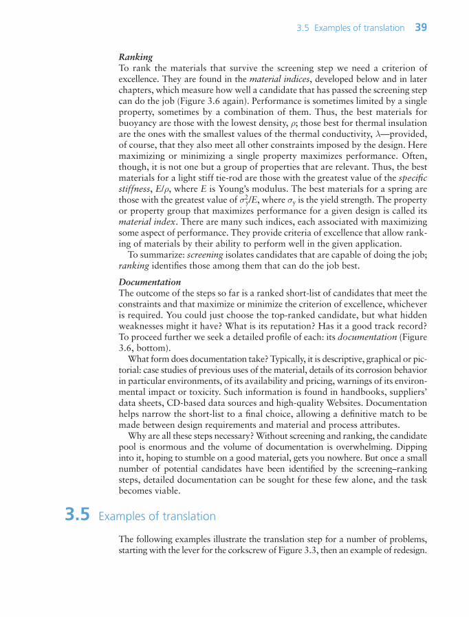
RankingTo rank the materials that survive the screening step we need a criterion ofexcellence. They are found in the material indices, developed below and in laterchapters, which measure how well a candidate that has passed the screening stepcan do the job (Figure 3.6 again). Performance is sometimes limited by a singleproperty, sometimes by a combination of them. Thus, the best materials forbuoyancy are those with the lowest density, ρ; those best for thermal insulationare the ones with the smallest values of the thermal conductivity, λ—provided,of course, that they also meet all other constraints imposed by the design. Heremaximizing or minimizing a single property maximizes performance. Often,though, it is not one but a group of properties that are relevant. Thus, the bestmaterials for a light stiff tie-rod are those with the greatest value of the specificstiffness, E/ρ, where E is Young’s modulus. The best materials for a spring arethose with the greatest value of σ2
y/E, where σy is the yield strength. The propertyor property group that maximizes performance for a given design is called itsmaterial index. There are many such indices, each associated with maximizingsome aspect of performance. They provide criteria of excellence that allow rank-ing of materials by their ability to perform well in the given application.
To summarize: screening isolates candidates that are capable of doing the job;ranking identifies those among them that can do the job best.
DocumentationThe outcome of the steps so far is a ranked short-list of candidates that meet theconstraints and that maximize or minimize the criterion of excellence, whicheveris required. You could just choose the top-ranked candidate, but what hiddenweaknesses might it have? What is its reputation? Has it a good track record?To proceed further we seek a detailed profile of each: its documentation (Figure3.6, bottom).
What form does documentation take? Typically, it is descriptive, graphical or pic-torial: case studies of previous uses of the material, details of its corrosion behaviorin particular environments, of its availability and pricing, warnings of its environ-mental impact or toxicity. Such information is found in handbooks, suppliers’data sheets, CD-based data sources and high-quality Websites. Documentationhelps narrow the short-list to a final choice, allowing a definitive match to bemade between design requirements and material and process attributes.
Why are all these steps necessary? Without screening and ranking, the candidatepool is enormous and the volume of documentation is overwhelming. Dippinginto it, hoping to stumble on a good material, gets you nowhere. But once a smallnumber of potential candidates have been identified by the screening–rankingsteps, detailed documentation can be sought for these few alone, and the taskbecomes viable.
3.5 Examples of translation
The following examples illustrate the translation step for a number of problems,starting with the lever for the corkscrew of Figure 3.3, then an example of redesign.
3.5 Examples of translation 39
Ch03-H8391.qxd 1/17/07 11:38 AM Page 39
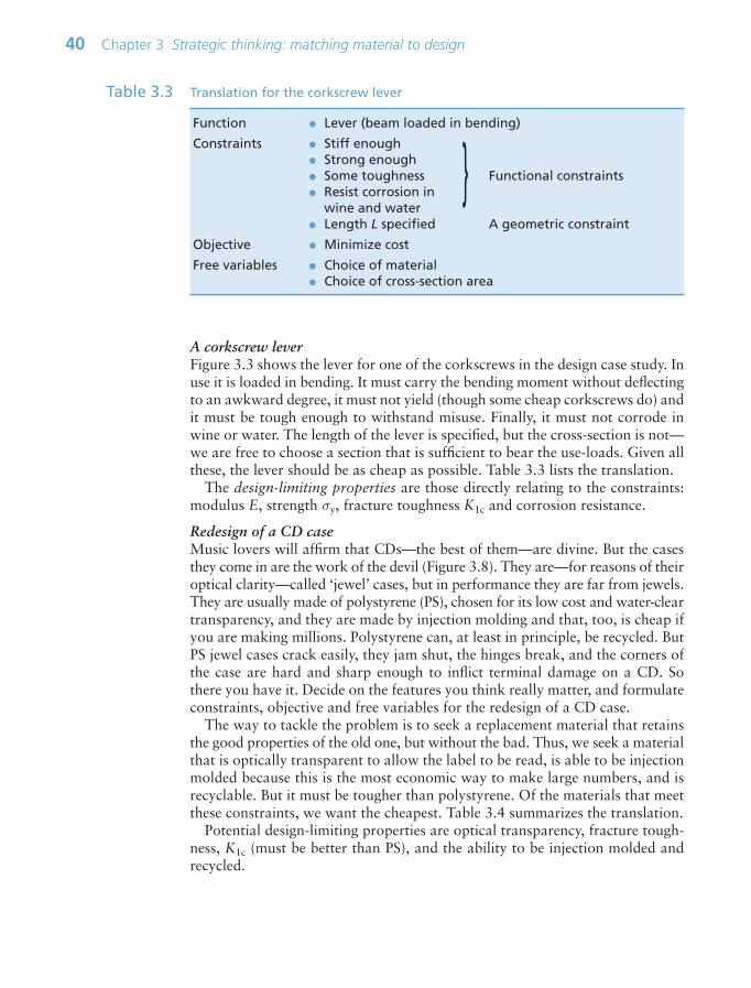
Function • Lever (beam loaded in bending)
Constraints • Stiff enough• Strong enough • Some toughness Functional constraints• Resist corrosion in
wine and water• Length L specified A geometric constraint
Objective • Minimize cost
Free variables • Choice of material• Choice of cross-section area
Table 3.3 Translation for the corkscrew lever
A corkscrew leverFigure 3.3 shows the lever for one of the corkscrews in the design case study. Inuse it is loaded in bending. It must carry the bending moment without deflectingto an awkward degree, it must not yield (though some cheap corkscrews do) andit must be tough enough to withstand misuse. Finally, it must not corrode inwine or water. The length of the lever is specified, but the cross-section is not—we are free to choose a section that is sufficient to bear the use-loads. Given allthese, the lever should be as cheap as possible. Table 3.3 lists the translation.
The design-limiting properties are those directly relating to the constraints:modulus E, strength σy, fracture toughness K1c and corrosion resistance.
Redesign of a CD caseMusic lovers will affirm that CDs—the best of them—are divine. But the casesthey come in are the work of the devil (Figure 3.8). They are—for reasons of theiroptical clarity—called ‘jewel’ cases, but in performance they are far from jewels.They are usually made of polystyrene (PS), chosen for its low cost and water-cleartransparency, and they are made by injection molding and that, too, is cheap ifyou are making millions. Polystyrene can, at least in principle, be recycled. ButPS jewel cases crack easily, they jam shut, the hinges break, and the corners ofthe case are hard and sharp enough to inflict terminal damage on a CD. Sothere you have it. Decide on the features you think really matter, and formulateconstraints, objective and free variables for the redesign of a CD case.
The way to tackle the problem is to seek a replacement material that retainsthe good properties of the old one, but without the bad. Thus, we seek a materialthat is optically transparent to allow the label to be read, is able to be injectionmolded because this is the most economic way to make large numbers, and isrecyclable. But it must be tougher than polystyrene. Of the materials that meetthese constraints, we want the cheapest. Table 3.4 summarizes the translation.
Potential design-limiting properties are optical transparency, fracture tough-ness, K1c (must be better than PS), and the ability to be injection molded andrecycled.
40 Chapter 3 Strategic thinking: matching material to design
Ch03-H8391.qxd 1/17/07 11:38 AM Page 40
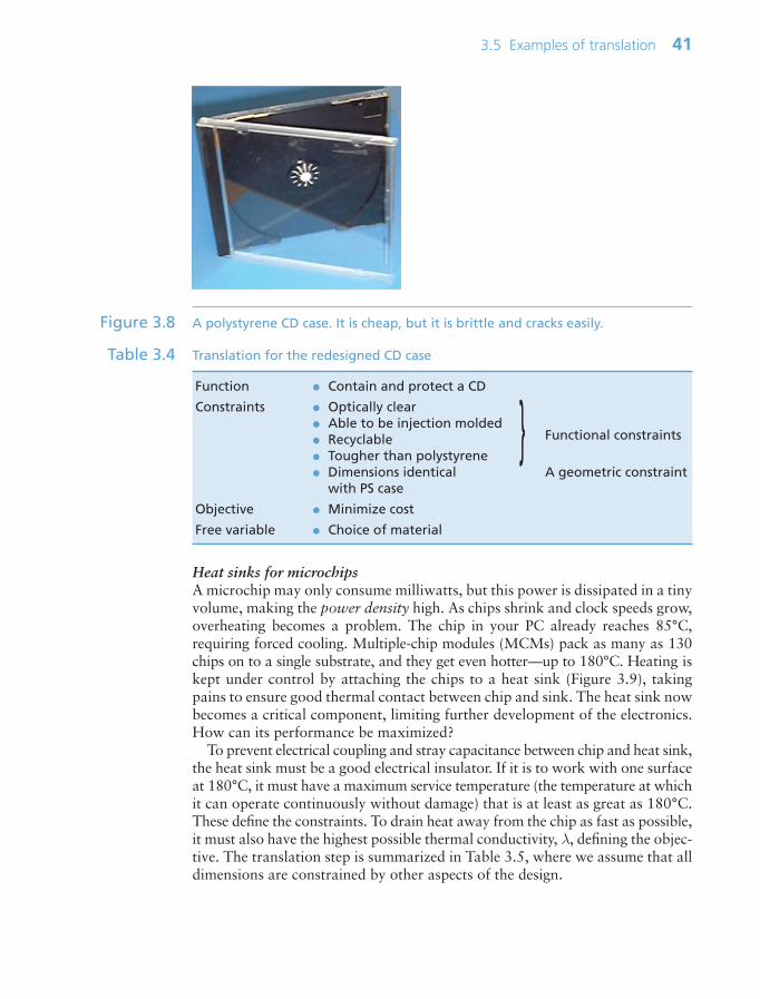
Heat sinks for microchipsA microchip may only consume milliwatts, but this power is dissipated in a tinyvolume, making the power density high. As chips shrink and clock speeds grow,overheating becomes a problem. The chip in your PC already reaches 85°C,requiring forced cooling. Multiple-chip modules (MCMs) pack as many as 130chips on to a single substrate, and they get even hotter—up to 180°C. Heating iskept under control by attaching the chips to a heat sink (Figure 3.9), takingpains to ensure good thermal contact between chip and sink. The heat sink nowbecomes a critical component, limiting further development of the electronics.How can its performance be maximized?
To prevent electrical coupling and stray capacitance between chip and heat sink,the heat sink must be a good electrical insulator. If it is to work with one surfaceat 180°C, it must have a maximum service temperature (the temperature at whichit can operate continuously without damage) that is at least as great as 180°C.These define the constraints. To drain heat away from the chip as fast as possible,it must also have the highest possible thermal conductivity, λ, defining the objec-tive. The translation step is summarized in Table 3.5, where we assume that alldimensions are constrained by other aspects of the design.
3.5 Examples of translation 41
Figure 3.8 A polystyrene CD case. It is cheap, but it is brittle and cracks easily.
Function • Contain and protect a CD
Constraints • Optically clear• Able to be injection molded Functional constraints• Recyclable• Tougher than polystyrene• Dimensions identical A geometric constraint
with PS case
Objective • Minimize cost
Free variable • Choice of material
Table 3.4 Translation for the redesigned CD case
Ch03-H8391.qxd 1/17/07 11:38 AM Page 41
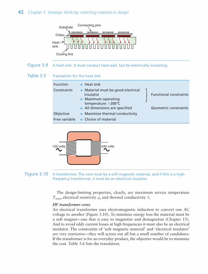
The design-limiting properties, clearly, are maximum service temperatureTmax, electrical resistivity ρe and thermal conductivity λ.
HF transformer coresAn electrical transformer uses electromagnetic induction to convert one ACvoltage to another (Figure 3.10). To minimize energy loss the material must bea soft magnet—one that is easy to magnetize and demagnetize (Chapter 15).And to avoid eddy current losses at high frequencies it must also be an electricalinsulator. The constraints of ‘soft magnetic material’ and ‘electrical insulator’are very restrictive—they will screen out all but a small number of candidates.If the transformer is for an everyday product, the objective would be to minimizethe cost. Table 3.6 lists the translation.
42 Chapter 3 Strategic thinking: matching material to design
Connecting pinsSubstrate
Chips
Cooling fins
Heatsink
Figure 3.9 A heat sink. It must conduct heat well, but be electrically insulating.
Function • Heat sink
Constraints • Material must be good electricalinsulator Functional constraints
• Maximum operatingtemperature 200°C
• All dimensions are specified Geometric constraints
Objective • Maximize thermal conductivity
Free variable • Choice of material
Table 3.5 Translation for the heat sink
120 volts 240 volts
Figure 3.10 A transformer. The core must be a soft magnetic material, and if this is a high-frequency transformer, it must be an electrical insulator.
Ch03-H8391.qxd 1/17/07 11:38 AM Page 42

These translations are the first step in selection. In them we have identified theconstraints; they will be used for screening. We have also identified the objective;it will be used for ranking. We will return to all four of these examples in laterchapters when we know how to screen and rank.
3.6 Summary and conclusions
The starting point of a design is a market need captured in a set of design require-ments. Concepts for a product that meet the need are devised. If initial estimatesand exploration of alternatives suggest that the concept is viable, the design pro-ceeds to the embodiment stage: working principles are selected, size and layoutare decided, and initial estimates of performance and cost are made. If the out-come is successful, the designer proceeds to the detailed design stage: optimizationof performance, full analysis of critical components, preparation of detailed pro-duction drawings (usually as a CAD file), showing dimensions, specifying preci-sion, and identifying material and manufacturing path. But design is not a linearprocess, as Figure 3.1 might suggest. Some routes lead to a dead end, requiringreiteration of earlier steps. And, frequently, the task is one of redesign, requir-ing that constraints be rethought and objectives realigned.
The selection of material and process runs parallel to this set of stages. Initiallythe search space for both is wide, encompassing all possible candidates. As thedesign requirements are formulated in increasing detail, constraints emerge thatboth must meet, and one or more objectives is formulated. The constraints nar-row the search space and the objective(s) allow ranking of those that remain.Identifying the constraints, the objectives and free variables (the process we called‘translation’) is the first step in selection. This chapter ended with examples oftranslation when the task was that of choosing a material; the exercises suggestmore. When the task is the choice of process, a similar translation is needed; wereturn to this in Chapter 18. The other steps—screening, ranking and docu-mentation—are discussed in chapters that follow.
3.7 Further reading
Ashby, M.F. (2005) Materials Selection in Mechanical Design, 3rd edition, Butterworth-Heinemann, Oxford, UK, Chapter 4. ISBN 0-7506-6168-2. (A more advanced textthat develops the ideas presented here in greater depth.)
3.7 Further reading 43
Function • HF transformer core
Constraints • Soft magnetic material Functional constraints• Electrical insulator• All dimensions are specified Geometric constraints
Objective • Minimize cost
Free variable • Choice of material
Table 3.6 Translation for the transformer core
Ch03-H8391.qxd 1/17/07 11:38 AM Page 43

Cross, N. (2000) Engineering Design Methods, 3rd edition, Wiley, Chichester, UK.ISBN 0-471-87250-3. (A durable text describing the design process, with emphasis ondeveloping and evaluating alternative solutions.)
French, M.J. (1985) Conceptual Design for Engineers, The Design Council, London,UK and Springer, Berlin, Germany. ISBN 0-85072-155-5 and 3-540-15175-3. (Theorigin of the ‘Concept—Embodiment—Detail’ block diagram of the design process.The book focuses on the concept stage, demonstrating how simple physical principlesguide the development of solutions to design problems.)
Pahl, G. and Beitz, W. (1997) Engineering design, 2nd edition, translated by K. Wallaceand L. Blessing, The Design Council, London, UK and Springer, Berlin, Germany.ISBN 0-85072-124-5 and 3-540-13601-0. (The Bible—or perhaps more exactly theOld Testament—of the technical design field, developing formal methods in the rigor-ous German tradition.)
Ullman, D.G. (2003) The Mechanical Design Process, 3rd edition, McGraw-Hill, New York, USA. ISBN 0-07-112281-8. (An American view of design, developingways in which an initially ill-defined problem is tackled in a series of steps, much inthe way suggested by Figure 3.1 of the present text.)
Ulrich, K.T. and Eppinger, S.D. (1995) Product Design and Development, McGraw-Hill,New York, USA. ISBN 0-07-065811-0. (A readable, comprehensible text on productdesign, as taught at MIT. Many helpful examples but almost no mention of materials.)
44 Chapter 3 Strategic thinking: matching material to design
Exercise E3.1 What are the steps in developing an original design?
Exercise E3.2 Describe and illustrate the ‘translation’ step of the material selection strategy.
Exercise E3.3 What is meant by an objective and what by a constraint in the requirementsfor a design? How do they differ?
Exercise E3.4 You are asked to design a fuel-saving cooking pan with the goal of wastingas little heat as possible while cooking. What objective would you choose,and what constraints would you think must be met?
Exercise E3.5 Bikes come in many forms, each aimed at a particular sector of the market:• Sprint bikes.• Touring bikes.• Mountain bikes.• Shopping bikes.• Children’s bikes.• Folding bikes.
Use your judgement to identify the primary objective and the constraints thatmust be met for each of these.
3.8 Exercises
Ch03-H8391.qxd 1/17/07 11:38 AM Page 44
3.8 Exercises 45
Exercise E3.6 A material is required for the windings of an electric air-furnace capable oftemperatures up to 1000°C. Think out what attributes a material must haveif it is to be made into windings and function properly in a furnace. List thefunction and the constraints; set the objective to ‘minimize material price’and the free variable to ‘choice of material’.
Exercise E3.7 A material is required to manufacture office scissors. Paper is an abrasivematerial and scissors sometimes encounter hard obstacles like staples. Listfunction and constraints; set the objective to ‘minimize material price’ and thefree variable to ‘choice of material’.
Exercise E3.8 A material is required for a heat exchanger to extract heat from geo-ther-mally heated, saline, water at 120°C (and thus under pressure). List functionand constraints; set the objective to ‘minimize material price’ and the free vari-able to ‘choice of material’.
Exercise E3.9 A material is required for a disposable fork for a fast-food chain. List the objec-tive and the constraints that you would see as important in this application.
Exercise E3.10 Formulate the constraints and objective you would associate with the choiceof material to make the forks of a racing bicycle.
Exercise E3.11 Cheap coat-hangers used to be made of wood—now it is only expensive onesthat use this material. Most coat-hangers are now metal or plastic, and bothdiffer in shape from the wooden ones, and from each other. Examine wood,metal and plastic coat-hangers, comparing the designs, and comment on theways in which the choice of material has influenced them.
Exercise E3.12 Cyclists carry water in bottles that slot into bottle holders on their bicycles.Examine metal and plastic bottle holders, comparing the designs, and com-ment on the ways in which the choice of material has influenced them.
Ch03-H8391.qxd 1/17/07 11:38 AM Page 45

3.9 Exploring design using CES
46 Chapter 3 Strategic thinking: matching material to design
The ‘Search’ facility of CES allows a full-text search of all records, identify-ing those that contain the search string. The default setting applies the searchto the Materials universe only. The pull-down menu headed ‘Look in table:’allows this to be reset to the Process universe or to All tables.
Exercise E3.13 A company wishes to enhance its image by replacing oil-based plastics in itsproducts by polymers based on natural materials. Use the ‘Search’ facility inCES to find biopolymers (search on ‘Biopolymer’). List the material you find.
Exercise E3.14 A maker of garden furniture is concerned that the competition is stealing partof his market with furniture made by RTM, a term with which he is unfamil-iar. Use the ‘Search’ facility in CES to find out what RTM is, and whether itis used to make things like garden furniture. (Remember that it is the Processuniverse that must be searched, since this is a process.)
Exercise E3.15 Use the ‘Search’ facility in CES to find materials for furnace windings.
Exercise E3.16 Use the ‘Search’ facility in CES to find materials for scissors and knife blades.
Exercise E3.17 Use the ‘Search’ facility in CES to find materials for heat exchangers.
Exercise E3.18 Use the ‘Search’ facility in CES to find materials for flooring.
Ch03-H8391.qxd 1/17/07 11:38 AM Page 46

Chapter 4Stiffness and weight: density
and elastic moduli
Tensilemember, or tie
Compressionmember, or column
Flexural member,or beam
Pressurevessel
Torsion member,or shaft
Tensile member, or tie Compression member,or column
Flexural member,or beam
Modes of loading. (Image of Stansted Airportcourtesy of Norman Foster and Partners, London, UK)
Chapter contents
4.1 Introduction and synopsis 484.2 Density, stress, strain and moduli 484.3 The big picture: material property charts 564.4 The science: what determines
density and stiffness? 584.5 Manipulating the modulus and density 694.6 Summary and conclusions 734.7 Further reading 744.8 Exercises 744.9 Exploring design with CES 774.10 Exploring the science with CES Elements 78
Ch04-H8391 1/17/07 10:46 AM Page 47

48 Chapter 4 Stiffness and weight: density and elastic moduli
4.1 Introduction and synopsis
Stress causes strain. If you are human, the ability to cope with stress withoutundue strain is called resilience. If you are a material, it is called elastic modulus.
Stress is something that is applied to a material by loading it. Strain—a changeof shape—is its response; it depends on the magnitude of the stress and the wayit is applied—the mode of loading. The cover picture illustrates the commonones. Ties carry tension—often, they are cables. Columns carry compression—tubes are more efficient as columns than solid rods because they don’t buckle aseasily. Beams carry bending moments, like the wing spar of the plane or the hor-izontal roof beams of the airport. Shafts carry torsion, as in the drive shaft ofcars or the propeller shaft of the plane. Pressure vessels contain a pressure, asin the tires of the plane. Often they are shells: curved, thin-walled structures.
Stiffness is the resistance to change of shape that is elastic, meaning that the material returns to its original shape when the stress is removed. Strength(Chapter 6) is its resistance to permanent distortion or total failure. Stress andstrain are not material properties; they describe a stimulus and a response.Stiffness (measured by the elastic modulus E, defined in a moment) and strength(measured by the elastic limit σy or tensile strength σts) are material properties.Stiffness and strength are central to mechanical design, often in combination withthe density, ρ. This chapter introduces stress and strain and the elastic modulithat relate them. These properties are neatly summarized in a material propertychart—the modulus–density chart—the first of many that we shall explore inthis book.
Density and elastic moduli reflect the mass of the atoms, the way they arepacked in a material and the stiffness of the bonds that hold them together. Thereis not much you can do to change any of these, so the density and moduli of purematerials cannot be manipulated at all. If you want to control these properties youcan either mix materials together, making composites, or disperse space withinthem, making foams. Property charts are a good way to show how this works.
4.2 Density, stress, strain and moduli
DensityMany applications (e.g. sports equipment, transport systems) require low weightand this depends in part on the density of the materials of which they are made.Density is mass per unit volume. It is measured in kg/m3 or sometimes, for con-venience, Mg/m3 (1 Mg/m3 1000 kg/m3).
The density of samples with regular shapes can be determined using precisionmass balance and accurate measurements of the dimensions (to give the volume),but this is not the best way. Better is the ‘double weighing’ method: the sample isfirst weighed in air and then when fully immersed in a liquid of known density.When immersed, the sample feels an upwards force equal to the weight of
Ch04-H8391 1/17/07 10:46 AM Page 48
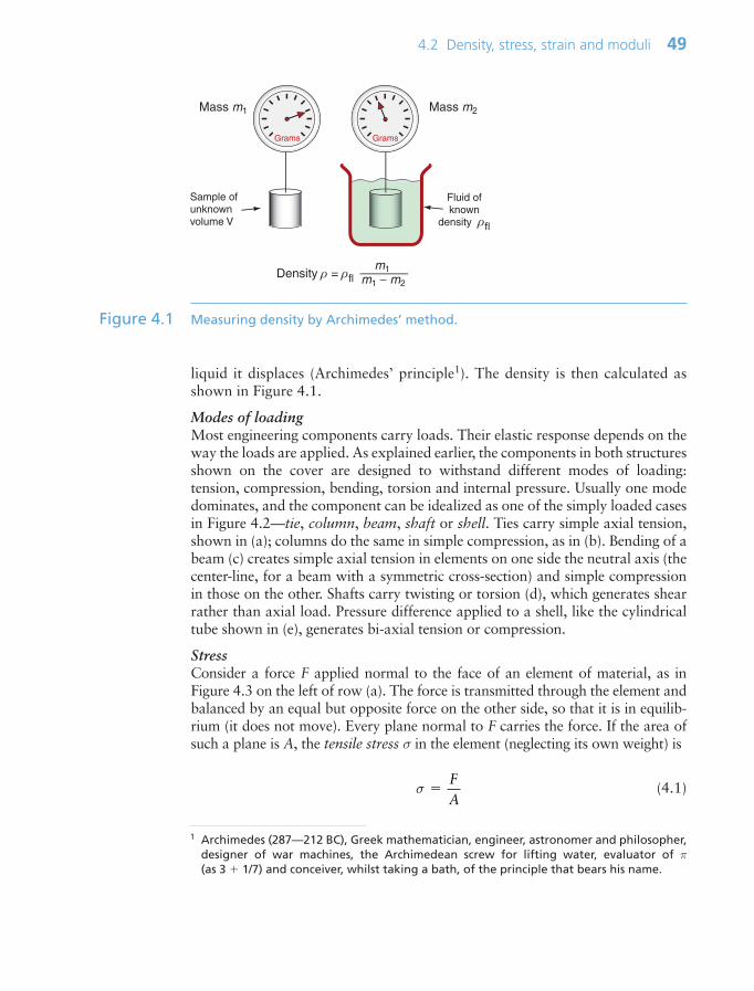
4.2 Density, stress, strain and moduli 49
liquid it displaces (Archimedes’ principle1). The density is then calculated asshown in Figure 4.1.
Modes of loadingMost engineering components carry loads. Their elastic response depends on theway the loads are applied. As explained earlier, the components in both structuresshown on the cover are designed to withstand different modes of loading: tension, compression, bending, torsion and internal pressure. Usually one modedominates, and the component can be idealized as one of the simply loaded casesin Figure 4.2—tie, column, beam, shaft or shell. Ties carry simple axial tension,shown in (a); columns do the same in simple compression, as in (b). Bending of abeam (c) creates simple axial tension in elements on one side the neutral axis (the center-line, for a beam with a symmetric cross-section) and simple compressionin those on the other. Shafts carry twisting or torsion (d), which generates shearrather than axial load. Pressure difference applied to a shell, like the cylindricaltube shown in (e), generates bi-axial tension or compression.
StressConsider a force F applied normal to the face of an element of material, as inFigure 4.3 on the left of row (a). The force is transmitted through the element andbalanced by an equal but opposite force on the other side, so that it is in equilib-rium (it does not move). Every plane normal to F carries the force. If the area ofsuch a plane is A, the tensile stress σ in the element (neglecting its own weight) is
(4.1)σ FA
Sample of unknown volume V
Grams Grams
Fluid of known
density ρfl
Mass m1 Mass m2
Density ρ = ρfl m1
m1 − m2
Figure 4.1 Measuring density by Archimedes’ method.
1 Archimedes (287—212 BC), Greek mathematician, engineer, astronomer and philosopher,designer of war machines, the Archimedean screw for lifting water, evaluator of π(as 3 1/7) and conceiver, whilst taking a bath, of the principle that bears his name.
Ch04-H8391 1/17/07 10:46 AM Page 49

50 Chapter 4 Stiffness and weight: density and elastic moduli
(a) A tie
F
F
F
F(b) A column (c) A beam
MM
(d) A shaft (e) A shell
po
p i
T T
Figure 4.2 Modes of loading and states of stress.
If the sign of F is reversed, the stress is compressive and given a negative sign.Forces2 are measured in newtons (N), so stress has the dimensions of N/m2. Buta stress of 1 N/m2 is tiny—atmospheric pressure is 105N/m2—so the usual unitis MN/m2 (106N/m2), called megapascals, symbol MPa3.
If, instead, the force lies parallel to the face of the element, three other forcesare needed to maintain equilibrium (Figure 4.3, row (b)). They create a state ofshear in the element. The shaded plane, for instance, carries the shear stress τ of
(4.2)
The units, as before, are MPa.One further state of multi-axial stress is useful in defining the elastic response
of materials: that produced by applying equal tensile or compressive forces toall six faces of a cubic element, as in Figure 4.3, row (c). Any plane in the cubenow carries the same state of stress—it is equal to the force on a cube facedivided by its area. The state of stress is one of hydrostatic pressure, symbol p,
τ F
As
2 Isaac Newton (1642–1727), scientific genius and alchemist, formulator of the laws ofmotion, the inverse-square law of gravity (though there is some controversy about this),laws of optics, the differential calculus, and much more.
3 Blaise Pascal (1623–1662), philosopher, mathematician and scientist, who took a certainpleasure in publishing his results without explaining how he reached them. Almost all,however, proved to be correct.
Ch04-H8391 1/17/07 10:46 AM Page 50

again with the units of MPa. There is an unfortunate convention here. Pressuresare positive when they push—the reverse of the convention for simple tensionand compression.
Engineering components can have complex shapes and can be loaded inmany ways, creating complex distributions of stress. But no matter how com-plex, the stresses in any small element within the component can always bedescribed by a combination of tension, compression and shear. Commonly thesimple cases of Figure 4.3 suffice, using superposition of two cases to capture,for example, bending plus compression.
StrainStrain is the response of materials to stress (second column of Figure 4.3). A tensile stress σ applied to an element causes the element to stretch. If the ele-ment in Figure 4.3(a), originally of side Lo, stretches by δL L Lo, the nom-inal tensile strain is
4.2 Density, stress, strain and moduli 51
Fs
FsFs
Area A
F
F
Area A
Tensile stress σ = F/A usual units MPa
Shear stress τ = Fs/A usual units MPa
p
p
p
p
pp
Pressure pusual units MPa
L
Lo
Tensile strain ε = (L − Lo)/Lo
Shear strain γ = w/Lo
Lo
w
Volume strain (dilatation) ∆ = (V −Vo)/Vo
Elastic deformationStress Strain
σ = E εE = Young’s modulus
τ = G γG = Shear modulus
p = K ∆K = Bulk modulus
Slope Eσ
ε
Slope Gτ
γ
Slope Kp
∆
(a)
(b)
(c)
Volume VVolume Vo
Figure 4.3 The definitions of stress, strain and elastic moduli.
Ch04-H8391 1/17/07 10:46 AM Page 51

(4.3)
A compressive stress shortens the element; the nominal compressive strain(negative) is defined in the same way. Since strain is the ratio of two lengths, itis dimensionless.
A shear stress causes a shear strain γ (Figure 4.3(b)). If the element shears bya distance w, the shear strain
(4.4)
In practice tan γ γ because strains are almost always small. Finally, a hydro-static pressure p causes an element of volume V to change in volume by δV. Thevolumetric strain, or dilatation (Figure 4.3(c)), is
(4.5)
Stress–strain curves and moduliFigure 4.4 shows typical tensile stress–strain curves for a ceramic, a metal anda polymer. The initial part, up to the elastic limit σel, is approximately linear(Hooke’s4 law), and it is elastic, meaning that the strain is recoverable—thematerial returns to its original shape when the stress is removed. Stresses above theelastic limit cause permanent deformation (ductile behavior) or brittle fracture.
Within the linear elastic regime, strain is proportional to stress (Figure 4.3,third column). The tensile strain is proportional to the tensile stress:
σ E (4.6)
and the same is true in compression. The constant of proportionality, E, iscalled Young’s5 modulus. Similarly, the shear strain γ is proportional to theshear stress τ:
τ Gγ (4.7)
and the dilatation ∆ is proportional to the pressure p:
p K∆ (4.8)
∆ δVV
tano
( )γ γwL
≈
ε δLLo
52 Chapter 4 Stiffness and weight: density and elastic moduli
4 Robert Hooke (1635–1703), able but miserable man, inventor of the microscope, and per-haps, too, of the idea of the inverse-square law of gravity. He didn’t get along with Newton.
5 Thomas Young (1773–1829), English scientist, expert on optics and deciphering ancientEgyptian hieroglyphs (among them, the Rosetta stone). It seems a little unfair that themodulus carries his name, not that of Hooke.
Ch04-H8391 1/17/07 10:46 AM Page 52

4.2 Density, stress, strain and moduli 53
Str
ess
σ =
F/A
o
FAo
FAo
L
*Elastic limit, σel (fracture)
Stress of order 300 MPa
Strain of order 0.0005
Slope E = σ/ε
Brittle ceramics
Str
ess
σ =
F/A
o
L
Ductile metals
Yield strength, σy
Slope E = σ/ε
Of order 300 MPa
Tensile strength, σts
*
Stress of order 500 MPa
Strain oforder 0.2
Str
ess
σ =
F/A
o
Strain ε = δL/L
Strain ε = δL/L
Strain ε = δL/L
FAo
L
Ductile polymers
Yield stress, σy
Slope E = σ/ε
*
Stress oforder 50 MPa
Strain of order 3.0
Figure 4.4 Tensile stress–strain curves for ceramics, metals and polymers.
Ch04-H8391 1/17/07 10:46 AM Page 53
where G is the shear modulus and K the bulk modulus, as illustrated in the thirdcolumn of Figure 4.3. All three of these moduli have the same dimensions as stress,that of force per unit area (N/m2 or Pa). As with stress it is convenient to use alarger unit, this time an even bigger one, that of 109 N/m2, gigapascals, or GPa.
Young’s modulus, the shear modulus and the bulk modulus are related, but torelate them we need one more quantity, Poisson’s6 ratio. When stretched in onedirection, the element of Figure 4.3(a) generally contracts in the other two direc-tions, as it is shown doing here. Poisson’s ratio, ν, is the negative of the ratio ofthe lateral or transverse strain, t, to the axial strain, , in tensile loading:
(4.9)
Since the transverse strain itself is negative, ν is positive—it is typically about 1/3.In an isotropic material (one for which the moduli do not depend on the direc-
tion in which the load is applied) the moduli are related in the following ways:
(4.10)
Commonly ν 1/3 when
(4.11a)
Elastomers are exceptional. For these ν 1/2 when
(4.11b)
This means that rubber (an elastomer) is easy to stretch in tension (low E), butif constrained from changing shape, or loaded hydrostatically, it is very stiff(large K)—a feature designers of shoes have to allow for.
Data sources like CES list values for all four moduli. In this book we exam-ine data for E; approximate values for the others can be derived from equations(4.11) when needed.
Elastic energyIf you stretch an elastic band, energy is stored in it. The energy can be consid-erable: catapults can kill people. The super-weapon of the Roman arsenal atone time was a wind-up mechanism that stored enough elastic energy to hurl a10 kg stone projectile 100 yards or more.
G E K E≈13
and
G E K E≈ ≈38
and
GE
KE
2 1 3 1 2( )
;( )ν ν
ν εεt
54 Chapter 4 Stiffness and weight: density and elastic moduli
6 Siméon Denis Poisson (1781–1840), French mathematician, known both for his constantand his distribution. He was famously uncoordinated, failed geometry at Universitybecause he could not draw, and had to abandon experimentation because of the disastersresulting from his clumsiness.
Ch04-H8391 1/17/07 10:46 AM Page 54
How do you calculate this energy? A force F acting through a displacementdL does work F dL. A stress σ F/A acting through a strain incrementd dL/L does work per unit volume
(4.12)
with units of J/m3. If the stress is acting on an elastic material, this work isstored as elastic energy. The elastic part of all three stress–strain curves ofFigure 4.4—the part of the curve before the elastic limit—is linear; in it σ E.The work done per unit volume as the stress is raised from zero to a final valueσ* is the area under the stress–strain curve:
(4.13)
This is the energy that is stored, per unit volume, in an elastically strained mate-rial. The energy is released when the stress is relaxed.
Measurement of Young’s modulusYou might think that the way to measure the elastic modulus of a materialwould be to apply a small stress (to be sure to remain in the linear elastic regionof the stress–strain curve), measure the strain and divide one by the other. Inreality, moduli measured as slopes of stress–strain curves are inaccurate, oftenby a factor of 2 or more, because of contributions to the strain from materialcreep or deflection of the test machine. Accurate moduli are measured dynam-ically: by measuring the frequency of natural vibrations of a beam or wire, orby measuring the velocity of sound waves in the material. Both depend onE/ρ, so if you know the density ρ you can calculate E.
Stress-free strainStress is not the only stimulus that causes strain. Certain materials respond toa magnetic field by undergoing strain—an effect known as magneto-striction.Others respond to an electrostatic field in the same way—they are known aspiezo-electric materials. In each case a material property relates the magnitudeof the strain to the intensity of the stimulus (Figure 4.5). The strains are smallbut can be controlled with great accuracy and, in the case of magneto-strictionand piezo-electric strain, can be changed with a very high frequency. This isexploited in precision positioning devices, acoustic generators and sensors—applications we return to in Chapters 14 and 15.
A more familiar effect is that of thermal expansion: strain caused by changeof temperature. The thermal strain T is linearly related to the temperaturechange ∆T by the expansion coefficient, α:
T α ∆T (4.14)
where the subscript ‘T ’ is a reminder that the strain is caused by temperaturechange, not stress.
WE E
σσ σ σσ σ
dd 1
2*
* *
ε0 0
2
∫ ∫( )
dd
dWF LAL
σ ε
4.2 Density, stress, strain and moduli 55
Ch04-H8391 1/17/07 10:46 AM Page 55

The term ‘stress-free strain’ is a little misleading. It correctly conveys the ideathat the strain is not caused by stress but by something else. But these strainscan none the less give rise to stresses if the body suffering the strain is con-strained. Thermal stress—stress arising from thermal expansion—particularly,can be a problem, causing mechanisms to jam and railway tracks to buckle. Weanalyze it in Chapter 12.
4.3 The big picture: material property charts
We met the idea of material property charts in Section 2.5. Now is the time touse them. If we want materials that are stiff and light, we first need an overviewof what’s available. What moduli do materials offer? What are their densities?The modulus–density chart shows them.
The modulus–density chartFigure 4.6 shows that the modulus E of engineering materials spans sevendecades7, from 0.0001 to nearly 1000 GPa; the density ρ spans a factor of2000, from less than 0.01 to 20 Mg/m3. The members of the ceramics and met-als families have high moduli and densities; none have a modulus less than10 GPa or a density less than 1.7 Mg/m3. Polymers, by contrast, all have mod-uli below 10 GPa and densities that are lower than those of any metal orceramic—most are close to 1 Mg/m3. Elastomers have roughly the same density
56 Chapter 4 Stiffness and weight: density and elastic moduli
Thermal field Expansioncoefficient
Piezo-electricconstant
Magnetostrictiveconstant
Elasticmoduli
Magnetic field
Electric field
Stress field
Strain
Stimulus
Materialproperty
Response
Figure 4.5 Stimuli leading to strain.
7 Very low density foams and gels (which can be thought of as molecular-scale, fluid-filled,foams) can have lower moduli than this. As an example, gelatine (as in Jello) has a modulusof about 105GPa.
Ch04-H8391 1/17/07 10:46 AM Page 56

as other polymers but their moduli are lower by a further factor of 100 ormore. Materials with a lower density than polymers are porous: man-madefoams and natural cellular structures like wood and cork.
This property chart gives an overview, showing where families and theirmembers lie in E–ρ space. It helps in the common problem of material selectionfor stiffness-limited applications in which weight must be minimized. More onthis in Chapter 5.
The modulus–relative cost chartOften it is minimizing cost, not weight, that is the overriding objective of a design.The chart of Figure 4.7 shows, on the x-axis, the relative prices per unit volume ofmaterials, normalized to that of the metal used in larger quantities than any other:mild steel. Concrete and wood are among the cheapest; polymers, steels and alu-minum alloys come next; special metals like titanium, most technical ceramics anda few polymers like PTFE and PEEK are expensive. The chart allows the selectionof materials that are stiff and cheap. Chapter 5 gives examples.
AnisotropyGlasses and most polymers have disordered structures with no particular direc-tionality about the way the atoms are arranged. They have properties that areisotropic, meaning the same no matter which direction they are measured.Most materials are crystalline—made up of ordered arrays of atoms. Metals
4.3 The big picture: material property charts 57
Density, ρ (Mg/m3)0.01
Yo
un
g’s
mo
du
lus,
E (
GP
a)
10−4
0.1 1 10
10−3
10−2
10−1
1
10
100
1000
Polyester
Foams
Polymers
Metals
Technicalceramics
Composites
Natural materials
Lead alloys
W alloys
SteelsTi alloys
Mg alloys
CFRP
GFRP
Al alloys
Rigid polymer foams
Flexible polymer foams
Ni alloys
Cu alloysyCu alloys
Zinc alloysPAPEEKPET
PMMA
PC
Cork
Wood
Butyl rubber
Silicone elastomers
Concrete
WC
Al2O3SiC
Si3N4Young’s modulus–Density
B4C
EpoxiesPS
PTFE
EVA
NeopreneIsoprene
Polyurethane
Leather
MFA, 07
PP
PE
Glass
// grain
grainT
Elastomers
Wood
Non-technicalceramics
Figure 4.6 The modulus–density chart.
Ch04-H8391 1/17/07 10:46 AM Page 57
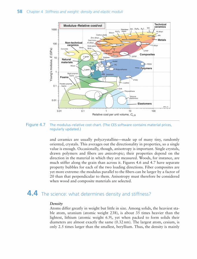
and ceramics are usually polycrystalline—made up of many tiny, randomly oriented, crystals. This averages out the directionality in properties, so a singlevalue is enough. Occasionally, though, anisotropy is important. Single crystals,drawn polymers and fibers are anisotropic; their properties depend on thedirection in the material in which they are measured. Woods, for instance, aremuch stiffer along the grain than across it. Figures 4.6 and 4.7 have separateproperty bubbles for each of the two loading directions. Fiber composites areyet more extreme: the modulus parallel to the fibers can be larger by a factor of20 than that perpendicular to them. Anisotropy must therefore be consideredwhen wood and composite materials are selected.
4.4 The science: what determines density and stiffness?
DensityAtoms differ greatly in weight but little in size. Among solids, the heaviest sta-ble atom, uranium (atomic weight 238), is about 35 times heavier than thelightest, lithium (atomic weight 6.9), yet when packed to form solids theirdiameters are almost exactly the same (0.32 nm). The largest atom, cesium, isonly 2.5 times larger than the smallest, beryllium. Thus, the density is mainly
58 Chapter 4 Stiffness and weight: density and elastic moduli
Relative cost per unit volume, Cv,R
You
ng’s
mod
ulus
, E (
GP
a)
0.01 0.1 1 10 100
0.01
0.1
1
10
100
1000
Foams
Polymers
Metals
Technicalceramics
Composites
Natural materials
Lead alloys
W alloys
Carbon steels
Ti alloys
Mg alloysCFRP
GFRP
Al alloys
Rigid polymer foams
Flexible polymer foams
Zinc alloys
PS
PTFE
PCWood
Silicone elastomers
Concrete
Al2O3
SiC Si3N4
Modulus–Relative cost/volB4C
PP
EVAPolyurethane
Leather
Non-technical ceramics
MFA, 07
Cast irons
WC
Soda glass
Silica glass
Silicon
Stone Brick
ABS
Epoxies
Ionomers
AlN
Stainless steels
PEEK
PE
PMMA
Polyurethanes
Acetal
// grain
grainT
Elastomers
Figure 4.7 The modulus–relative cost chart. (The CES software contains material prices,regularly updated.)
Ch04-H8391 1/17/07 10:46 AM Page 58

determined by the atomic weight and is influenced to a lesser degree by the atomsize and the way in which they are packed. Metals are dense because they aremade of heavy atoms, packed densely together (iron, for instance, has an atomicweight of 56). Polymers have low densities because they are largely made of lightcarbon (atomic weight: 12) and hydrogen (atomic weight: 1) in low-densityamorphous or semi-crystalline packings. Ceramics, for the most part, have lowerdensities than metals because they contain light Si, O, N or C atoms. Even thelightest atoms, packed in the most open way, give solids with a density of around1 Mg/m3—the same as that of water (see Figure 4.6). Materials with lower densi-ties than this are foams, made up of cells containing a large fraction of pore space.
Atom packing in metals and the unit cellAtoms often behave as if they were hard, spherical balls. The balls on a pooltable, when set, are arranged as a close-packed layer, as in Figure 4.8(a). Theatoms of many metals pack in this way, forming layers that are far more exten-sive. There is no way to pack atoms more closely than this, so this particulararrangements is called ‘close packed’. Atomic structures are close packed notjust in two dimensions but in three. Surprisingly, there are two ways to do this.The depressions where three atoms meet in the first layer, layer A, allow theclosest nesting for a second layer, B. A third layer can be added such that itsatoms are exactly above those in the first layer, so that it, too, is in the A orien-tation, and the sequence repeated to give a crystal with ABABAB . . . stacking,as in Figure 4.8(b); it is called close packed hexagonal, or CPH (or sometimesHCP) for short, for reasons explained in a moment. There is also an alterna-tive. In placing the second layer, layer B, there are two choices of position. If thethird layer, C, is nested onto B so that it lies in the alternative position, the stack-ing becomes (on repeating) ABCABCABC . . . as shown in (c) in the figure; it iscalled face-centered cubic or FCC for short. Many metals, such as copper, silver,aluminum and nickel, have the FCC structure; many others, such as magnesium,zinc and titanium, have the CPH structure. The two alternative structures have
4.4 The science: what determines density and stiffness? 59
(a) Close-packed layer A (b) Layer B on layer A to give ABABAB ... or CPH packing
(c) Layer C on layers A and B to give ABCABC ... or FCC packing
Figure 4.8 (a) A close-packed layer of spheres, layer A; atoms often behave as if hard andspherical. (b) A second layer, B, nesting in the first; repeating this sequence givesABAB . . . or CPH stacking. (c) A third layer, C, can be nested so that it does notlie above A or B; if repeated this gives ABCABC . . . or FCC stacking.
Ch04-H8391 1/17/07 10:46 AM Page 59

exactly the same packing fraction, 0.74, meaning that the spheres occupy 74%of the available space. But the small difference in layout influences properties,particularly those to do with plastic deformation (Chapter 6).
Not all structures are close packed. Figure 4.9 shows one of these, made bystacking square-packed layers with a lower packing density than the hexagonallayers of the FCC and HCP structures. An ABABAB . . . stacking of these lay-ers builds the body-centered cubic structure, BCC for short, with a packingfraction of 0.68. Iron and most steels have this structure. There are many othercrystal structures, but for now these three are enough.
Any regular packing of atoms that repeats itself is called a crystal. It is poss-ible to pack atoms in a non-crystallographic way to give what is called an amor-phous structure, sketched in Figure 4.10. This is not such an efficient way to fillspace with spheres: the packing fraction is 0.64 at best.
The characterizing unit of a crystal structure is called its unit cell. Figure 4.11shows three; the red lines define the cell (the atoms have been shrunk to revealit more clearly). In the first, shown in (a), the cell is a hexagonal prism. Theatoms in the top, bottom and central planes form close-packed layers like that
60 Chapter 4 Stiffness and weight: density and elastic moduli
(a) Non-close-packed layer A (b) Layer B on layer A to give ABABAB... or BCC packing
Figure 4.9 (a) A square grid of spheres; it is a less efficient packing than that of the previousfigure. (b) A second layer, B, nesting in the first, A; repeating this sequence givesABAB . . . packing. If the sphere spacing is adjusted so that the gray spheres lie on the corners of a cube, the result is the non-close-packed BCC structure.
(a) A non-crystallographic layer A
(b) An amorphous or non-crystallographic structure
Figure 4.10 (a) An irregular arrangement of spheres. (b) Extending this in three dimensionsgives a random or amorphous structure.
Ch04-H8391 1/17/07 10:46 AM Page 60

of Figure 4.8(b), with ABAB . . . stacking. For these reasons, the structure is calledclose-packed hexagonal (CPH). The second, shown in (b), is also made up ofclose-packed layers, though this is harder to see: the shaded triangular plane isone of them. If we think of this as an A plane, atoms in the plane above it nest inthe B position and those in the plane above that, in the C, giving ABCABC . . .stacking, as in Figure 4.8(c). The unit cell itself is a cube with an atom at each cor-ner and one at the center of each face—for this reason it is called face-centeredcubic (FCC). The final cell, shown in (c), is the characterizing unit of the square-layer structure of Figure 4.9; it is a cube with an atom at each corner and one inthe middle, and is called, appropriately, body-centered cubic (BCC).
Unit cells pack to fill space as in Figure 4.12; the resulting array is called thecrystal lattice; the points at which cell edges meet are called lattice points. The
4.4 The science: what determines density and stiffness? 61
(b) The FCC unit cell (c) The BCC unit cell(a) The CPH unit cell
Figure 4.11 Unit cells. All the atoms are of the same type, but are shaded differently toemphasize their positions. (a) The close-packed hexagonal (CPH) structure. (b) The close-packed face-centered cubic (FCC) structure. (c) The non-close-packed body-centered cubic (BCC) structure. Arrows show nearest neighbors.
(a) (b) (c)
Figure 4.12 Unit cells stacked to fill space. (a) The hexagonal cell. (b) The cubic cell. (c) A cellwith edges of differing length that do not meet at right angles.
Ch04-H8391 1/17/07 10:46 AM Page 61
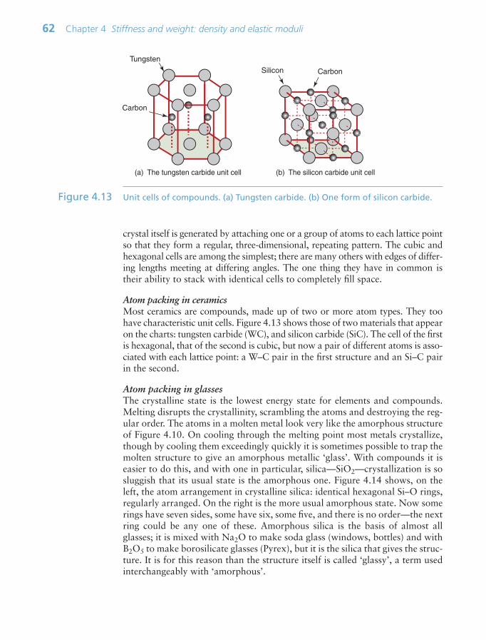
crystal itself is generated by attaching one or a group of atoms to each lattice pointso that they form a regular, three-dimensional, repeating pattern. The cubic andhexagonal cells are among the simplest; there are many others with edges of differ-ing lengths meeting at differing angles. The one thing they have in common istheir ability to stack with identical cells to completely fill space.
Atom packing in ceramicsMost ceramics are compounds, made up of two or more atom types. They toohave characteristic unit cells. Figure 4.13 shows those of two materials that appearon the charts: tungsten carbide (WC), and silicon carbide (SiC). The cell of the firstis hexagonal, that of the second is cubic, but now a pair of different atoms is asso-ciated with each lattice point: a W–C pair in the first structure and an Si–C pairin the second.
Atom packing in glassesThe crystalline state is the lowest energy state for elements and compounds.Melting disrupts the crystallinity, scrambling the atoms and destroying the reg-ular order. The atoms in a molten metal look very like the amorphous structureof Figure 4.10. On cooling through the melting point most metals crystallize,though by cooling them exceedingly quickly it is sometimes possible to trap themolten structure to give an amorphous metallic ‘glass’. With compounds it iseasier to do this, and with one in particular, silica—SiO2—crystallization is sosluggish that its usual state is the amorphous one. Figure 4.14 shows, on theleft, the atom arrangement in crystalline silica: identical hexagonal Si–O rings,regularly arranged. On the right is the more usual amorphous state. Now somerings have seven sides, some have six, some five, and there is no order—the nextring could be any one of these. Amorphous silica is the basis of almost allglasses; it is mixed with Na2O to make soda glass (windows, bottles) and withB2O5 to make borosilicate glasses (Pyrex), but it is the silica that gives the struc-ture. It is for this reason than the structure itself is called ‘glassy’, a term usedinterchangeably with ‘amorphous’.
62 Chapter 4 Stiffness and weight: density and elastic moduli
(a) The tungsten carbide unit cell
Tungsten
Carbon
(b) The silicon carbide unit cell
Silicon Carbon
Figure 4.13 Unit cells of compounds. (a) Tungsten carbide. (b) One form of silicon carbide.
Ch04-H8391 1/17/07 10:46 AM Page 62

Atom packing in polymersPolymer structures are quite different. The backbone of a ‘high’ polymer (‘high’means high molecular weight) is a long chain of carbon atoms, to which sidegroups are attached. Figure 4.15 shows a segment of the simplest: polyethylene,PE, (!CH2!)n. The chains have ends; the ends of this one are capped with aCH3 group. PE is made by the polymerization (snapping together) of ethylenemolecules, CH2RCH2; the R symbol is a double bond, broken by polymeriza-tion to give the links to more carbon neighbors to the left and right. Figure 4.16shows the chain structure of five of the most widely used linear polymers.
Polymer molecules bond together to form solids. The chains of a linear polymer,103 to 106 !CH2! units in length, are already strongly bonded along the chainitself. Separated chains attract each other, but weakly so (Figure 4.17(a))—theyare sticky, but not very sticky; the ‘hydrogen’ bonds that make them stick areeasily broken or rearranged. The resulting structure is sketched in Figure4.18(a): a dense spaghetti-like tangle of molecules with no order or crystallinity;it is amorphous. This is the structure of thermoplastics like those of Figure 4.16;the weak bonds melt easily, allowing the polymer to be molded, retaining itsnew shape on cooling.
4.4 The science: what determines density and stiffness? 63
(a) Crystalline (b) Amorphous
Silicon
Oxygen Oxygen
Silicon
Figure 4.14 Two alternative structures for silica, the basis of most glasses. (a) Crystallinesilica. (b) Glassy or amorphous silica.
Carbon Hydrogen
– C – C – C – C – C – C – C – C –
H
-
H
H
-
H
H
-
H
H
-
H
H
-
H
H
-
H
H
-
H
H
-
H–
(– CH2 –)n
Figure 4.15 Polymer chains have a carbon–carbon backbone with hydrogen or other sidegroups. The figure shows three alternative representations of the polyethylenemolecule.
Ch04-H8391 1/17/07 10:46 AM Page 63

64 Chapter 4 Stiffness and weight: density and elastic moduli
– C – C – C – C – C – C – C – C –H
–
H
–
H
–
H
–
H
–
H
–
H
–
H
–
H
–
H
–
H
–
H
–
H
–
H
–
H
–
H
–– C – C – C – C – C – C – C – C –
F F F
–
F
–
–
F
–
–
F
–
F
–
F
–
F
–
F
–
F
–
F
–
F
–
F
–
F–
F
–
– C – C – C – C – C – C – C – C –H
–
H
–
H
–
Cl
–
H
–
H
–
Cl
–
H
–
H–
H
–H
–
Cl
–
H
–H
–
Cl
–
H
–
CH3CH3
– C – C – C – C – C – C – C – C –H
–
H
–
H
–
H
–
H
– –
H
––C6H5
– C – C – C – C – C – C – C – C –H
–
H
–
H–
H
–
H
–
H–
H
–
H
–
H
––
–
H
–
H
–
H
––
–
C6H5
C6H5
CH3 CH3H–
H
–
H
–
H
– –
H
–
H
––C6H5
Polyethylene, PE
Polypropylene, PP
Polystyrene, PS
Polyvinyl chloride, PVC
Polytetrafluoroethylene, PTFE
Figure 4.16 Five common polymers, showing the chemical make-up. The strongcarbon–carbon bonds are shown in red.
Strong covalent bond
Weak hydrogenbond
Strong covalent bond
Strong covalentcross-link
(b)
(a)
Figure 4.17 (a) Polymer chains have strong covalent ‘backbones’, but bond to each otheronly with weak hydrogen bonds unless they become cross-linked. (b) Cross-linksbond the chains tightly together. The strong carbon–carbon bonds are shown assolid red lines.
Ch04-H8391 1/17/07 10:46 AM Page 64

The weak bonds of thermoplastics, do, however, try to line molecules up, as theyare shown in Figure 4.17(a). The molecules are so long that total alignment is notpossible, but segments of molecules manage it, giving small crystalline regions, asin Figure 4.18(b). These crystallites, as they are called, are small—often between 1and 10 µm across, just the right size to scatter light. So amorphous polymers withno crystallites can be transparent—polycarbonate (PC), polymethyl-methacrylate(PMMA; Plexiglas) and polystyrene (PS) are examples. Those with some crys-tallinity, like polyethylene (PE) and nylon (PA), scatter light and are translucent.
The real change comes when chains are cross-linked by replacing some of theweak hydrogen bonds by much more muscular covalent C!C bonds, as in Figure4.17(b), making the whole array into one huge, multiply connected network.Elastomers (rubbery polymers) have relatively few cross-links, as in Figure 4.18(c).
4.4 The science: what determines density and stiffness? 65
(a) Non-cross-linked
Polymer chains
Cross-links
(d) Highly cross-linked
Cross-links
(c) Slightly cross-linked
AmorphousCrystallite
(b) Partly crystalline
Figure 4.18 (a) Chains in polymers like polypropylene form spaghetti-like tangles with noregular repeating pattern—that structure is amorphous or ‘glassy’. (b) Somepolymers have the ability to form regions in which the chains line up andregister, giving crystalline patches. The sketch shows a partly crystalline polymerstructure. (c) Elastomers have occasional cross-links between chains, but theseare far apart, allowing the chains between them to stretch. (d) Heavily cross-linkedpolymers like epoxy inhibit chain sliding.
Ch04-H8391 1/17/07 10:46 AM Page 65

Thermosets like epoxies and phenolics have many cross-links, as in Figure 4.18(d),making them stiffer and stronger than thermoplastics. The cross-links are not bro-ken by heating, so once the links have formed thermosets cannot be thermallymolded or (for that reason) recycled.
Cohesive energy and elastic moduli: crystals and glassesAtoms bond together, some weakly, some strongly. The cohesive energy meas-ures the strength of this bonding. It is defined as the energy per mol (a mol is6 1023 atoms) required to separate the atoms of a solid completely, givingneutral atoms at infinity. Equally it is the energy released if the neutral, widelyspaced atoms are brought together to form the solid.
The greater the cohesive energy, the stronger are the bonds between the atomsand the higher is the modulus. Think of the bonds as little springs (Figure 4.19).The atoms have equilibrium spacing ao; a force F pulls them apart a little, toao δ, but when it is released they jump back to their original spacing. The samehappens in compression because the potential energy of the bond increases nomatter which direction the force is applied, as the curve in the figure suggests.The bond energy is a minimum at the equilibrium spacing. A spring that stretchesby δ under a force F has a stiffness, S, of
(4.15)
and this is the same in compression as in tension.
SF
δ
66 Chapter 4 Stiffness and weight: density and elastic moduli
Force F
Displacement δ
Displacement δ
Springstiffness S
Energy U
Energy U = F δ/2
Tension
Compression
Equilibriumatom position
ao
ao+ δ
F F
0
Figure 4.19 Atoms in crystals and glasses are linked by atomic bonds that behave likesprings. The bond stiffness is S F/δ. Stretching or compressing the bond by adisplacement δ stores energy U Fδ/2. The equilibrium (no force) atomseparation is at the bottom of the energy well.
Ch04-H8391 1/17/07 10:46 AM Page 66
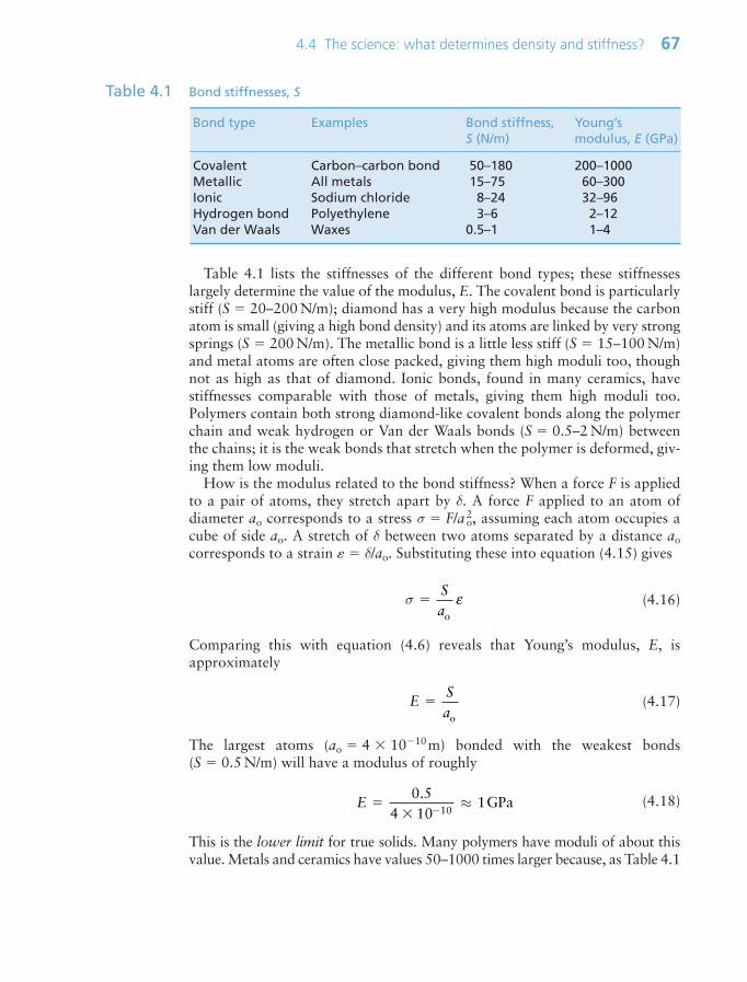
Table 4.1 lists the stiffnesses of the different bond types; these stiffnesseslargely determine the value of the modulus, E. The covalent bond is particularlystiff (S 20–200 N/m); diamond has a very high modulus because the carbonatom is small (giving a high bond density) and its atoms are linked by very strongsprings (S 200 N/m). The metallic bond is a little less stiff (S 15–100 N/m)and metal atoms are often close packed, giving them high moduli too, thoughnot as high as that of diamond. Ionic bonds, found in many ceramics, havestiffnesses comparable with those of metals, giving them high moduli too.Polymers contain both strong diamond-like covalent bonds along the polymerchain and weak hydrogen or Van der Waals bonds (S 0.5–2 N/m) betweenthe chains; it is the weak bonds that stretch when the polymer is deformed, giv-ing them low moduli.
How is the modulus related to the bond stiffness? When a force F is appliedto a pair of atoms, they stretch apart by δ. A force F applied to an atom ofdiameter ao corresponds to a stress σ F/a2
o, assuming each atom occupies acube of side ao. A stretch of δ between two atoms separated by a distance aocorresponds to a strain δ/ao. Substituting these into equation (4.15) gives
(4.16)
Comparing this with equation (4.6) reveals that Young’s modulus, E, isapproximately
(4.17)
The largest atoms (ao 4 1010m) bonded with the weakest bonds(S 0.5 N/m) will have a modulus of roughly
(4.18)
This is the lower limit for true solids. Many polymers have moduli of about thisvalue. Metals and ceramics have values 50–1000 times larger because, as Table 4.1
E
0 54 10
110
.≈ GPa
ESa
o
σ Sao
ε
4.4 The science: what determines density and stiffness? 67
Bond type Examples Bond stiffness, Young’s S (N/m) modulus, E (GPa)
Covalent Carbon–carbon bond 50–180 200–1000Metallic All metals 15–75 60–300Ionic Sodium chloride 8–24 32–96Hydrogen bond Polyethylene 3–6 2–12Van der Waals Waxes 0.5–1 1–4
Table 4.1 Bond stiffnesses, S
Ch04-H8391 1/17/07 10:46 AM Page 67
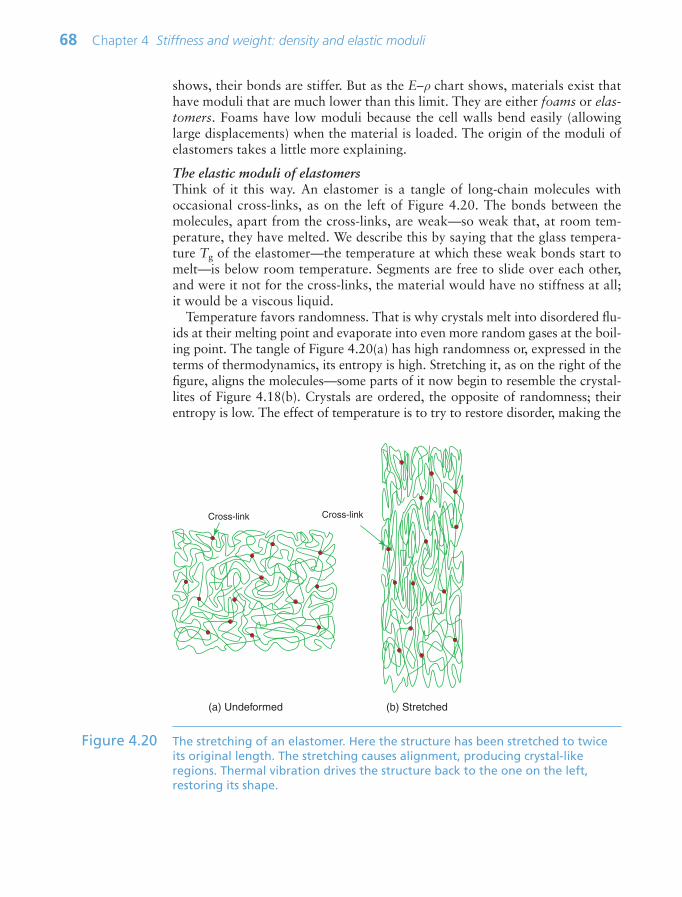
shows, their bonds are stiffer. But as the E–ρ chart shows, materials exist thathave moduli that are much lower than this limit. They are either foams or elas-tomers. Foams have low moduli because the cell walls bend easily (allowinglarge displacements) when the material is loaded. The origin of the moduli ofelastomers takes a little more explaining.
The elastic moduli of elastomersThink of it this way. An elastomer is a tangle of long-chain molecules withoccasional cross-links, as on the left of Figure 4.20. The bonds between themolecules, apart from the cross-links, are weak—so weak that, at room tem-perature, they have melted. We describe this by saying that the glass tempera-ture Tg of the elastomer—the temperature at which these weak bonds start tomelt—is below room temperature. Segments are free to slide over each other,and were it not for the cross-links, the material would have no stiffness at all;it would be a viscous liquid.
Temperature favors randomness. That is why crystals melt into disordered flu-ids at their melting point and evaporate into even more random gases at the boil-ing point. The tangle of Figure 4.20(a) has high randomness or, expressed in theterms of thermodynamics, its entropy is high. Stretching it, as on the right of thefigure, aligns the molecules—some parts of it now begin to resemble the crystal-lites of Figure 4.18(b). Crystals are ordered, the opposite of randomness; theirentropy is low. The effect of temperature is to try to restore disorder, making the
68 Chapter 4 Stiffness and weight: density and elastic moduli
Cross-link
(a) Undeformed (b) Stretched
Cross-link
Figure 4.20 The stretching of an elastomer. Here the structure has been stretched to twiceits original length. The stretching causes alignment, producing crystal-likeregions. Thermal vibration drives the structure back to the one on the left,restoring its shape.
Ch04-H8391 1/17/07 10:46 AM Page 68

material revert to a random tangle, and the cross-links give it a ‘memory’ of thedisordered shape it had to start with. So there is a resistance to stretching—astiffness—that has nothing to do with bond stretching, but with strain-inducedordering. A full theory is complicated—it involves the statistical mechanics of long-chain tangles—so it is not easy to calculate the value of the modulus.The main thing to know is that the moduli of elastomers are low because theyhave this strange origin and that they increase with temperature (because of theincreasing tendency to randomness), whereas those of true solids decrease(because of thermal expansion).
Mixtures of atomsMost engineering materials are not pure but contain two or more different ele-ments. Often they dissolve in each other, like sugar in tea, but as the material issolid we call it a solid solution—examples are brass (a solution of zinc in cop-per), solder (a solution of tin in lead) and stainless steel (a solution of nickel andchromium in iron).
As we shall see later, some material properties are changed a great deal bymaking solid solutions. Modulus and density are not. As a general rule the den-sity ρ of a solid solution lies between the densities ρA and ρB of the materialsthat make it up, following a rule of mixtures (an arithmetic mean, weighted byvolume fraction) known, in this instance, as Vegard’s law:
(4.19)
where f is the fraction of A atoms. Modulus is a bit more complicated—purematerials have only one kind of bond, A!A say; mixtures of A and B atomshave three: A!A, B!B and A!B. Within each bond type of Table 4.1 the stiff-ness ranges are not large, so mixtures of bonds again average out to valuesbetween those of the pure elements.
Alloying is not therefore a route to manipulating the modulus and densityvery much. To do this, mixtures must be made at a more macroscopic scale tomake a hybrid material. We can mix two discrete solids together to make com-posites, or we can mix in some space to make foams. The effects on modulusand density are illustrated via the property chart in the next section.
4.5 Manipulating the modulus and density
CompositesComposites are made by embedding fibers or particles in a continuous matrixof a polymer (polymer matrix composites, PMCs), a metal (MMCs) or a ceramic(CMCs), as in Figure 4.21. The development of high-performance compositesis one of the great material developments of the last 40 years, now reachingmaturity. Composites have high stiffness and strength per unit weight, and—inthe case of MMCs and CMCs—high temperature performance. Here, then, weare interested in stiffness and weight.
ρ ρ ρ f fA B( )1
4.5 Manipulating the modulus and density 69
Ch04-H8391 1/17/07 10:46 AM Page 69
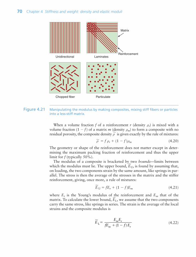
When a volume fraction f of a reinforcement r (density ρr) is mixed with a volume fraction (1 f ) of a matrix m (density ρm) to form a composite with noresidual porosity, the composite density ρ is given exactly by the rule of mixtures:
ρ f ρr (1 f )ρm (4.20)
The geometry or shape of the reinforcement does not matter except in deter-mining the maximum packing fraction of reinforcement and thus the upperlimit for f (typically 50%).
The modulus of a composite is bracketed by two bounds—limits betweenwhich the modulus must lie. The upper bound, E
U, is found by assuming that,
on loading, the two components strain by the same amount, like springs in par-allel. The stress is then the average of the stresses in the matrix and the stifferreinforcement, giving, once more, a rule of mixtures:
E
U fEr (1 f )Em (4.21)
where Er is the Young’s modulus of the reinforcement and Em that of thematrix. To calculate the lower bound, E
L, we assume that the two components
carry the same stress, like springs in series. The strain is the average of the localstrains and the composite modulus is
(4.22)EE E
fE f Em r
m r
L
( )1
70 Chapter 4 Stiffness and weight: density and elastic moduli
Chopped fiber Particulate
Unidirectional Laminates
Matrix
Reinforcement
Figure 4.21 Manipulating the modulus by making composites, mixing stiff fibers or particlesinto a less-stiff matrix.
Ch04-H8391 1/17/07 10:46 AM Page 70

Figure 4.22 shows the range of composite properties that could, in principle,be obtained by mixing two materials together—the boundaries are calculatedfrom equations (4.20)–(4.22). Composites can therefore fill in some of the oth-erwise empty spaces on the E–ρ chart, opening up new possibilities in design.There are practical limits of course—the matrix and reinforcement must bechemically compatible and available in the right form, and processing the mix-ture must be achievable at a sensible cost. Fiber-reinforced polymers are well-established examples—Figure 4.6 shows GFRP and CFRP, sitting in the compositesbubble between the polymers bubble and the ceramics bubble. They are as stiffas metals, but lighter.
FoamsFoams are made much as you make bread: by mixing a matrix material (thedough) with a foaming agent (the yeast), and controlling what then happens insuch a way as to trap the bubbles. Polymer foams are familiar as insulation andflotation and as the filler in cushions and packaging. You can, however, makefoams from other materials: metals, ceramics and even glass. They are light forthe obvious reason that they are, typically, 90% space, and they have low mod-uli. This might make them sound as though they are of little use, but that is mis-taken: if you want to cushion or to protect a delicate object (such as yourself)what you need is a material with a low, controlled, stiffness and strength. Foamsprovide it.
4.5 Manipulating the modulus and density 71
Density, ρ (Mg/m3)
Yo
un
g’s
mo
du
lus,
E (
GP
a)
10–1
1
1 10
10
100
1000
Polymers
Er
Em
ρrρm
Eu
El
Matrix m
Reinforcement r
Ceramics
Figure 4.22 Composites made from a matrix m with a reinforcement r have moduli anddensities, depending on the volume fraction and form of the reinforcement,that lie within the gray shaded lozenge bracketed by equations (4.21) and(4.22). Here the matrix is a polymer and the reinforcement a ceramic, but thesame argument holds for any combination.
Ch04-H8391 1/17/07 10:46 AM Page 71

Figure 4.23 shows an idealized cell of a low-density foam. It consists of solidcell walls or edges surrounding a void containing a gas. Cellular solids are char-acterized by their relative density, the fraction of the foam occupied by thesolid. For the structure shown here (with t L) it is
(4.23)ρρ
s
tL
⎛
⎝⎜⎜⎜
⎞
⎠⎟⎟⎟⎟
2
72 Chapter 4 Stiffness and weight: density and elastic moduli
Opencell face
Cell edge
t
L
t
FF
F
F
Cell edgebending
δ
L
L
L
L
Figure 4.23 Manipulating the modulus by making a foam—a lattice of material with celledges that bend when the foam is loaded.
Density, ρ (Mg/m3)
Yo
un
g’s
mo
du
lus,
E (
GP
a)
0.01 0.1 110−4
10−3
10−2
10−1
1
10
Polymers
Foams
Elastomers
Foam with relative density 0.1
Solid polymer
Es
ρsρ
E
Factor 10
Factor 100
Figure 4.24 Foaming creates new materials with lower modulus and density. Low modulus is good for making packaging and protective shielding; low density is good forlightweight design and for flotation. The red arrow is a plot of equation (4.24).
Ch04-H8391 1/17/07 10:46 AM Page 72

where ρ is the density of the foam, ρs is the density of the solid of which it ismade, L is the cell size and t is the thickness of the cell edges.
When the foam is loaded, the cell walls bend, as shown on the right of thefigure. This behavior can be modeled (we will be able to do so by the end of thenext chapter), giving the foam modulus E
:
(4.24)
where Es is the modulus of the solid from which the foam is made. This givesus a second way of manipulating the modulus, in this case, decreasing it. At arelative density of 0.1 (meaning that 90% of the material is empty space), themodulus of the foam is only 1% of that of the material in the cell wall, assketched in Figure 4.24. The range of modulus and density for real foams isillustrated in the chart of Figure 4.6—as expected, they fall below and to theleft of the polymers of which they are made.
4.6 Summary and conclusions
When a solid is loaded, it initially deforms elastically. ‘Elastic’ means that,when the load is removed, the solid springs back to its original shape. Thematerial property that measures stiffness is the elastic modulus—and becausesolids can be loaded in different ways, we need three of them:
• Young’s modulus, E, measuring resistance to stretching;• the shear modulus, G, measuring resistance to twisting; and• the bulk modulus, K, measuring the resistance to hydrostatic compression.
Many applications require stiffness at low weight, particularly ground, air andspace vehicles, and that means a high modulus and a low density.
The density of a material is the weight of its atoms divided by the volumethey occupy. Atoms do not differ much in volume, but they differ a great dealin weight. Thus, the density is principally set by the atomic weight; the furtherdown the Periodic Table we go the greater becomes the density.
The moduli have their origins in the stiffness of the bonds between atoms in asolid and in the number of atoms (and thus bonds) per unit volume. The atomicvolume, as we have said, does not vary much from one solid to another, so themoduli mainly reflect the stiffness of the bonds. Bonding can take several forms,depending on how the electrons of the atoms interact. The metallic, covalent andionic bonds are generally stiff, hydrogen and Van der Waals bonds are much lessso—that is why steel has high moduli and polyethylene has low.
There is very little that can be done to change the bond stiffness or atomicweight of a solid, so at first sight we are stuck with the moduli and densities ofthe materials we already have. But there are two ways to manipulate them: by
EE
s s
ρρ
⎛
⎝⎜⎜⎜⎜
⎞
⎠⎟⎟⎟⎟⎟
2
4.6 Summary and conclusions 73
Ch04-H8391 1/17/07 10:46 AM Page 73
mixing two materials to make composites, or by mixing a material with spaceto make foams. Both are powerful ways of creating ‘new’ materials that occupyregions of the E–ρ map that were previously empty.
4.7 Further reading
Ashby, M.F. and Jones, D.R.H. (2006) Engineering Materials 1, 3rd edition, ElsevierButterworth-Heinemann, Oxford, UK. ISBN 0-7506-6380-4. (One of a pair of intro-ductory texts dealing with the engineering properties and processing of materials.)
Askeland, D.R. and Phule, P.P. (2006) The Science of Engineering Materials, 5th edition,Thompson Publishing, Toronto, Canada. (A mature text dealing with the science ofmaterials, and taking a science-led rather than a design-led approach.)
Callister, W.D. Jr (2007) Materials Science and Engineering, An Introduction, 7th edi-tion, Wiley, New York, USA. ISBN 0-471-73696-1. (A long established and highlyrespected introduction to materials, taking the science-based approach.)
74 Chapter 4 Stiffness and weight: density and elastic moduli
4.8 Exercises
Exercise E4.1 Identify which of the five modes of loading (Figure 4.2) is dominant in thefollowing components:
• Fizzy drinks container.• Overhead electric cable.• Shoe soles.• Wind turbine blade.• Climbing rope.• Bicycle forks.• Aircraft fuselage.
Can you think of another example for each mode of loading?
Exercise E4.2 The cable of a hoist has a cross-section of 80 mm2. The hoist is used to lift acrate weighing 500 kg. What is the stress in the cable? The free length of thecable is 3 m. How much will it extend if it is made of steel (modulus200 GPa)? How much if it is made of polypropylene, PP (modulus 1.2 GPa)?
Exercise E4.3 Water has a density of 1000 kg/m3. What is the hydrostatic pressure at adepth of 100 m?
Exercise E4.4 A catapult has two rubber arms, each with a square cross-section with a width4 mm and length 300 mm. In use its arms are stretched to three times their orig-inal length before release. Assume the modulus of rubber is 103GPa and thatit does not change when the rubber is stretched. How much energy is stored inthe catapult just before release?
Ch04-H8391 1/17/07 10:46 AM Page 74
4.8 Exercises 75
Exercise E4.5 Use the modulus–density chart of Figure 4.6 to find, from among the materi-als that appear on it:
(a) The material with the highest density.(b) The metal with the lowest modulus.(c) The polymer with the highest density.(d) The approximate ratio of the modulus of woods measured parallel to the
grain and perpendicular to the grain.(e) The approximate range of modulus of elastomers.
Exercise E4.6 Use the modulus–relative cost chart of Figure 4.7 to find, from among thematerials that appear on it:
(a) The cheapest material with a modulus greater than 1 GPa.(b) The cheapest metal.(c) The cheapest polymer.(d) Whether magnesium alloys are more or less expensive than aluminum
alloys.(e) Whether PEEK (a high-performance engineering polymer) is more or less
expensive than PTFE.
Exercise E4.7 What is meant by:
• A crystalline solid?• An amorphous solid?• A thermoplastic?• A thermoset?• An elastomer?
Exercise E4.8 The stiffness S of an atomic bond in a particular material is 50 N/m and itscenter-to-center atom spacing is 0.3 nm. What, approximately, is its elasticmodulus?
Exercise E4.9 Derive the upper and lower bounds for the modulus of a composite quotedas in equations (4.21) and (4.22) of the text. To derive the first, assume thatthe matrix and reinforcement behave like two springs in parallel (so thateach must strain by the same amount), each with a stiffness equal to its mod-ulus E multiplied by its volume fraction, f. To derive the second, assume thatthe matrix and reinforcement behave like two springs in series (so that bothare stressed by the same amount), again giving each a stiffness equal to itsmodulus E multiplied by its volume fraction, f.
Exercise E4.10 A volume fraction f 0.2 of silicon carbide (SiC) particles is combined with analuminum matrix to make a metal matrix composite. The modulus and densityof the two materials are listed in the table. The modulus of particle-rein-forced composites lies very close to the lower bound, equation (4.22), dis-cussed in the text. Calculate the density and approximate modulus of the
Ch04-H8391 1/17/07 10:46 AM Page 75

76 Chapter 4 Stiffness and weight: density and elastic moduli
composite. Is the specific modulus, E/ρ, of the composite greater than that ofunreinforced aluminum? How much larger is the specific modulus if thesame volume fraction of SiC in the form of continuous fibers is used instead?For continuous fibers the modulus lies very close to the upper bound, equa-tion (4.21).
Exercise E4.11 Read the modulus E for polypropylene (PP) from the E–ρ chart of Figure 4.6.Estimate the modulus of a PP foam with a relative density ρ~/ρs of 0.2.
Density (Mg/m3) Modulus (GPa)
Aluminum 2.70 70Silicon carbide 3.15 420
Ch04-H8391 1/17/07 10:46 AM Page 76

4.9 Exploring design with CES 77
4.9 Exploring design with CES (use Level 2, Materials, throughout)
Exercise E4.12 Make an E–ρ chart using the CES software. Use a box selection to find threematerials with densities between 1000 and 3000 kg/m3 and the highest possiblemodulus.
Exercise E4.13 Data estimation. The modulus E is approximately proportional to the melt-ing point Tm in Kelvin (because strong inter-atomic bonds give both stiffnessand resistance to thermal disruption). Use CES to make an E–Tm chart for metals and estimate a line of slope 1 through the data for materials. Usethis line to estimate the modulus of cobalt, given that it has a melting pointof 1760 K.
Exercise E4.14 Sanity checks for data. A text reports that nickel, with a melting point of1720 K, has a modulus of 5500 GPa. Use the E–Tm correlation of the previousquestion to check the sanity of this claim. What would you expect it to be?
Exercise E4.15 Explore the potential of PP–SiC (polypropylene–silicon carbide) fiber com-posites in the following way. Make a modulus–density (E–ρ) chart andchange the axis ranges so that they span the range 1 E 1000 GPa and500 ρ 5000 kg/m3. Find and label PP and SiC, then print it. Retrievevalues for the modulus and density of PP and of SiC from the records forthese materials (use the means of the ranges). Calculate the density ρ and upperand lower bounds for the modulus E
at a volume fraction f of SiC of 0.5 and
plot this information on the chart. Sketch by eye two arcs starting from (E,ρ) for PP, passing through each of the (E
, ρ) points you have plotted and end-
ing at the (E, ρ) point for SiC. PP–SiC composites can populate the areabetween the arcs roughly up to f 0.5 because it is not possible to insertmore than this.
Exercise E4.16 Explore the region that can be populated by making PP foams. Expand an E–ρplot so that it spans the range 104 E 10 GPa and 10 ρ 2000 kg/m3.Find and label PP, then print the chart. Construct a band starting with the PPbubble by drawing lines corresponding to the scaling law for foam modulusE
ρ2 (equation 4.24) touching the top and the bottom of the PP bubble.The zone between these lines can be populated by PP foams.
Ch04-H8391 1/17/07 10:46 AM Page 77
78 Chapter 4 Stiffness and weight: density and elastic moduli
4.10 Exploring the science with CES Elements
Exercise E4.17 The text cited the following approximate relationships between the elasticconstants Young’s modulus, E, the shear modulus, G, the bulk modulus, Kand Poisson’s ratio, ν:
Use CES to make plots with the bit on the left-hand side of each equation onone axis and the bit on the right on the other. To do this you will need to usethe ‘Advanced’ facility in the dialog box for choosing the axes to create func-tions on the right of the two equations. How good an approximation are they?
Exercise E4.18 The cohesive energy Hc is the energy that binds atoms together in a solid.Young’s modulus E measures the force needed to stretch the atomic bondsand the melting point, Tm, is a measure of the thermal energy needed to dis-rupt them. Both derive from the cohesion, so you might expect E and Tm tobe related. Use CES to plot one against the other to see (use absolute meltingpoint, not centigrade or fahrenheit).
Exercise E4.19 The force required to stretch an atomic bond is
where dH is the change in energy of the bond when it is stretched by da. Thisforce corresponds to a stress
The modulus E is
The binding energy per atom in a crystal, Ha, is
HH
Nac
A
Ea a a
Ha a
dd
dd
ddo o o
σ σε ( / ) ( / )
13
2
2
σ Fa a
Ha a
Ha ao o o o
dd
dd2 2 3
1 1( / )
FHa
dd
GE
KE
2 1 3 1 2( )
;( )ν ν
Ch04-H8391 1/17/07 10:46 AM Page 78
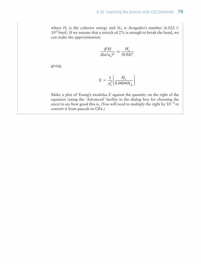
4.10 Exploring the science with CES Elements 79
where Hc is the cohesive energy and NA is Avogadro’s number (6.022 1023/mol). If we assume that a stretch of 2% is enough to break the bond, wecan make the approximation:
giving
Make a plot of Young’s modulus E against the quantity on the right of theequation (using the ‘Advanced’ facility in the dialog box for choosing theaxes) to see how good this is. (You will need to multiply the right by 109 toconvert it from pascals to GPa.)
Ea
H
N
10 00043
o
c
A.
⎛
⎝⎜⎜⎜⎜
⎞
⎠⎟⎟⎟⎟⎟
dd o
c2
2 20 02H
a a
H
( / ) ( . )≈
Ch04-H8391 1/17/07 10:46 AM Page 79

This page intentionally left blank

Chapter 5Flex, sag and wobble:
stiffness-limited design
Chapter contents
5.1 Introduction and synopsis 825.2 Standard solutions to elastic problems 825.3 Material indices for elastic design 895.4 Plotting limits and indices on charts 955.5 Case studies 995.6 Summary and conclusions 1065.7 Further reading 1075.8 Exercises 1075.9 Exploring design with CES 1095.10 Exploring the science with CES
Elements 109
A pole vaulter – the pole stores elastic energy. (Imagecourtesy of Gill Athletics, 2808 Gemini Court,
Champaign, IL 61822-9648, USA)
Ch05-H8391 1/17/07 10:45 AM Page 81
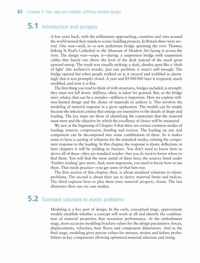
82 Chapter 5 Flex, sag and wobble: stiffness-limited design
5.1 Introduction and synopsis
A few years back, with the millennium approaching, countries and cites aroundthe world turned their minds to iconic building projects. In Britain there were sev-eral. One was—well, is—a new pedestrian bridge spanning the river Thames,linking St Paul’s Cathedral to the Museum of Modern Art facing it across theriver. The design was—oops, is—daring: a suspension bridge with suspensioncables that barely rise above the level of the deck instead of the usual greatupward sweep. The result was visually striking: a sleek, slender, span like a ‘shaftof light’ (the architect’s words). Just one problem: it wasn’t stiff enough. Thebridge opened but when people walked on it, it swayed and wobbled so alarm-ingly that it was promptly closed. A year and $5 000 000 later it reopened, muchmodified, and now it is fine.
The first thing you tend to think of with structures, bridges included, is strength:they must not fall down. Stiffness, often, is taken for granted. But, as the bridgestory relates, that can be a mistake—stiffness is important. Here we explore stiff-ness-limited design and the choice of materials to achieve it. This involves themodeling of material response in a given application. The models can be simplebecause the selection criteria that emerge are insensitive to the details of shape andloading. The key steps are those of identifying the constraints that the materialmust meet and the objective by which the excellence of choice will be measured.
We saw at the beginning of Chapter 4 that there are certain common modes ofloading: tension, compression, bending and torsion. The loading on any realcomponent can be decomposed into some combination of these. So it makessense to have a catalog of solutions for the standard modes, relating the compo-nent response to the loading. In this chapter, the response is elastic deflection; inlater chapters it will be yielding or fracture. You don’t need to know how toderive all of these—they are standard results—but you do need to know where tofind them. You will find the most useful of them here; the sources listed under‘Further reading’ give more. And, most important, you need to know how to usethem. That needs practice—you get some of that here too.
The first section of this chapter, then, is about standard solutions to elasticproblems. The second is about their use to derive material limits and indices.The third explains how to plot them onto material property charts. The lastillustrates their use via case studies.
5.2 Standard solutions to elastic problems
Modeling is a key part of design. In the early, conceptual stage, approximatemodels establish whether a concept will work at all and identify the combina-tion of material properties that maximize performance. At the embodimentstage, more accurate modeling brackets values for the design parameters: forces,displacements, velocities, heat fluxes and component dimensions. And in thefinal stage, modeling gives precise values for stresses, strains and failure proba-bilities in key components allowing optimized material selection and sizing.
Ch05-H8391 1/17/07 10:45 AM Page 82
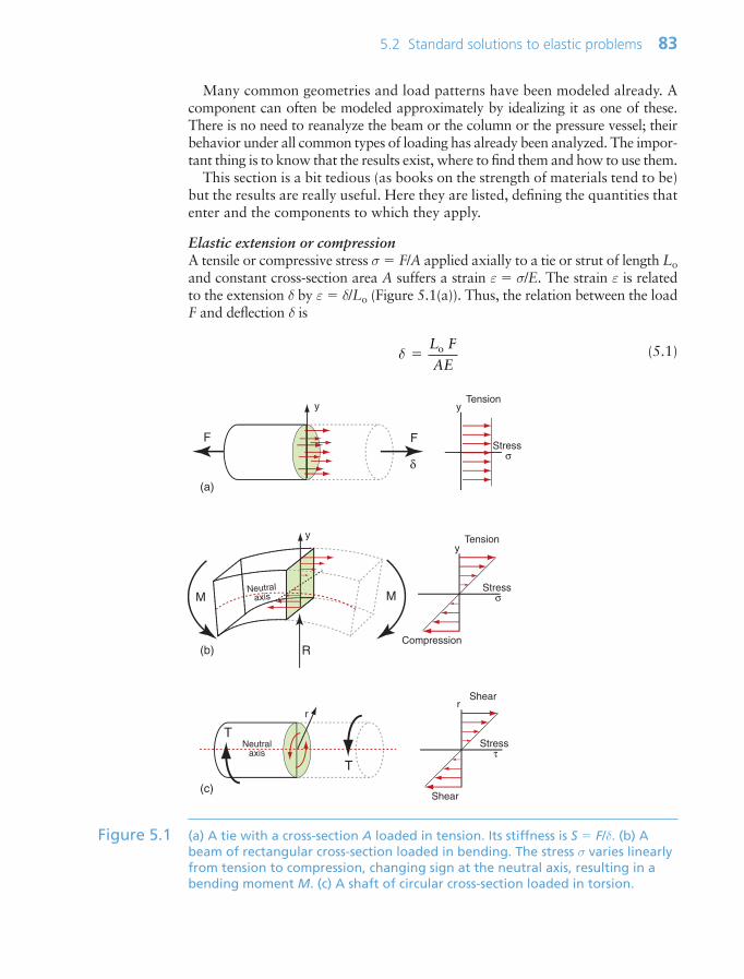
5.2 Standard solutions to elastic problems 83
Many common geometries and load patterns have been modeled already. Acomponent can often be modeled approximately by idealizing it as one of these.There is no need to reanalyze the beam or the column or the pressure vessel; theirbehavior under all common types of loading has already been analyzed. The impor-tant thing is to know that the results exist, where to find them and how to use them.
This section is a bit tedious (as books on the strength of materials tend to be)but the results are really useful. Here they are listed, defining the quantities thatenter and the components to which they apply.
Elastic extension or compressionA tensile or compressive stress σ F/A applied axially to a tie or strut of length Loand constant cross-section area A suffers a strain ε σ/E. The strain ε is relatedto the extension δ by ε δ/Lo (Figure 5.1(a)). Thus, the relation between the loadF and deflection δ is
(5.1)δ L F
AEo
Stress σ
yTension
y
FF
δ
(a)
R
yy
Tension
Compression
M MNeutral
axisStress
σ
(b)
rr
Stress τ
Neutralaxis
Shear
Shear(c)
T
T
Figure 5.1 (a) A tie with a cross-section A loaded in tension. Its stiffness is S F/δ. (b) Abeam of rectangular cross-section loaded in bending. The stress σ varies linearlyfrom tension to compression, changing sign at the neutral axis, resulting in abending moment M. (c) A shaft of circular cross-section loaded in torsion.
Ch05-H8391 1/17/07 10:45 AM Page 83
The stiffness S is defined as
(5.2)
Note that the shape of the cross-section area does not matter because the stressis uniform over the section.
Elastic bending of beamsWhen a beam is loaded by a bending moment M, its initially straight axis isdeformed to a curvature κ (Figure 5.1(b))
where u is the displacement parallel to the y-axis. The curvature generates a lin-ear variation of axial strain ε (and thus stress σ) across the section, with tensionon one side and compression on the other—the position of zero stress being theneutral axis. The stress increases with distance y from the neutral axis. Materialis more effective at resisting bending the further it is from that axis, so theshape of the cross-section is important. Elastic beam theory gives the stress σcaused by a moment M in a beam made of material of Young’s modulus E, as
(5.3)
where I is the second moment of area, defined as
(5.4)
The distance y is measured vertically from the neutral axis and b(y) is the widthof the section at y. The moment I characterizes the resistance of the section tobending—it includes the effect of both size and shape. Examples for four com-mon sections are listed in Figure 5.2 with expressions for the cross-section areaA and the second moment of area, I.
I y b y y 2section
( ) d∫
Eu
x
dd
2
2
σκ
yMI
E
κ dd
2
2
ux
SF AE
L
δ o
84 Chapter 5 Flex, sag and wobble: stiffness-limited design
Ch05-H8391 1/17/07 10:45 AM Page 84

5.2 Standard solutions to elastic problems 85
Section shape Area Am
Moment Im42
Moment Km4
bh12hb 3
)bh(
)hb58 .01(
3hb 3
−
2rπ 4r4π 4r
2π
tr2
)rr( 2i
20
π-π
tr
)rr(4
3
4i
40
π
−π
tr2
)rr(2
3
4i
40
π
−π
h
b
2r
2ro
t
2ri
h
b
t4
22 )
ht
1((b +h)
hbt2
2t (h+b)(h,b >>t)
h3t (1 3 ) hb
61
Figure 5.2 Cross-section area and second moments of sections for four section shapes.
48
F, δ
3845
3
C1L
F, δ
F, δ
Figure 5.3 Elastic deflection of beams. The deflection δ of a span L under a force F dependson the flexural stiffness EI of the cross-section and the way the force isdistributed. The constant C1 is defined in equation (5.5).
The ratio of moment to curvature, M/κ, is called the flexural rigidity, EI. Figure5.3 shows three possible distributions of load F, each creating a distribution ofmoment M(x). The maximum deflection, δ, is found by integrating equation (5.3)twice for a particular M(x). For a beam of length L with a transverse load F, the
Ch05-H8391 1/17/07 10:45 AM Page 85

stiffness is
(5.5)
The result is the same for all simple distributions of load; the only thing thatdepends on the distribution is the value of the constant C1; the figure lists val-ues for the three distributions. We will find in Section 5.3 that the best choiceof material is independent of the value of C1 with the happy result that the bestchoice for a complex distribution of loads is the same as that for a simple one.
Torsion of shaftsA torque, T, applied to the ends of an isotropic bar of uniform section gener-ates a shear stress τ (Figures 5.1(c) and 5.4). For circular sections, the shearstress varies with radial distance r from the axis of symmetry is
(5.6)
where K measures the resistance of the section to twisting (the torsional equiv-alent to I, for bending). K is easiest to calculate for circular sections, when it isequal to the polar second moment of area:
(5.7)
where r is measured radially from the center of the circular section. For non-circular sections, K is less than J. Figure 5.2 gives expressions for K for fourstandard shapes.
J r r 2 d3section
π∫
τr
TK
SF C EI
L
δ1
3
86 Chapter 5 Flex, sag and wobble: stiffness-limited design
T,θT
T,θT
L
Figure 5.4 Elastic torsion of circular shafts. The stress in the shaft and the twist per unitlength depend on the torque T and the torsional rigidity GK.
Ch05-H8391 1/17/07 10:45 AM Page 86

The shear stress acts in the plane normal to the axis of the bar. It causes thebar, with length L, to twist through an angle θ. The twist per unit length, θ/L,is related to the shear stress and the torque by
(5.8)
where G is the shear modulus. The ratio of torque to twist, T/θ, per unit length,is equal to GK, called the torsional rigidity.
Buckling of columns and plateIf sufficiently slender, an elastic column or plate, loaded in compression, fails byelastic buckling at a critical load, Fcrit. Beam theory shows that the criticalbuckling load depends on the length L and flexural rigidity, EI:
(5.9)
where n is a constant that depends on the end constraints: clamped, or free torotate, or free also to translate (Figure 5.5). The value of n is just the numberof half-wavelengths of the buckled shape (the half-wavelength is the distancebetween inflection points).
Some of the great engineering disasters have been caused by buckling. It canoccur without warning and slight misalignment is enough to reduce the load atwhich it happens. When dealing with compressive loads on columns or in-plane compression of plates it is advisable to check that you are well away fromthe buckling load.
Fn EI
Lcrit
2 2
2
π
τ θr
TK
GL
5.2 Standard solutions to elastic problems 87
1
nL
12
F
F
2F
Figure 5.5 The buckling load of a column of length L depends on the flexural rigidity EIand on the end constraints; three are shown here, together with the value of n.
Ch05-H8391 1/17/07 10:45 AM Page 87
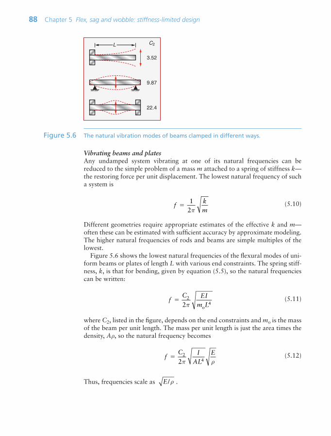
Vibrating beams and platesAny undamped system vibrating at one of its natural frequencies can bereduced to the simple problem of a mass m attached to a spring of stiffness k—the restoring force per unit displacement. The lowest natural frequency of sucha system is
(5.10)
Different geometries require appropriate estimates of the effective k and m—often these can be estimated with sufficient accuracy by approximate modeling.The higher natural frequencies of rods and beams are simple multiples of thelowest.
Figure 5.6 shows the lowest natural frequencies of the flexural modes of uni-form beams or plates of length L with various end constraints. The spring stiff-ness, k, is that for bending, given by equation (5.5), so the natural frequenciescan be written:
(5.11)
where C2, listed in the figure, depends on the end constraints and mo is the massof the beam per unit length. The mass per unit length is just the area times thedensity, Aρ, so the natural frequency becomes
(5.12)
Thus, frequencies scale as .E/ρ
fC I
ALE
242π ρ
fC EI
m L 2
o42π
fkm
1
2π
88 Chapter 5 Flex, sag and wobble: stiffness-limited design
L
3.52
C2
9.87
22.4
Figure 5.6 The natural vibration modes of beams clamped in different ways.
Ch05-H8391 1/17/07 10:45 AM Page 88

5.3 Material indices for elastic design
We can now start to implement the steps outlined in Chapter 3 and summa-rized in Figure 3.6:
• Translation• Screening, based on constraints• Ranking, based on objectives, and• Documentation to give greater depth.
The first two were fully described in Chapter 3. The third—ranking based onobjectives—requires simple modeling to identify the material index.
An objective, it will be remembered, is a criterion of excellence for the designas a whole, something to be minimized (like cost, weight or volume) or maxi-mized (like energy storage). Here we explore those for elastic design.
Minimizing weight: a light, stiff tie-rodThink first of choosing a material for a cylindrical tie-rod like one of those inthe cover picture of Chapter 4. Its length Lo is specified and it must carry a ten-sile force F without extending elastically by more than δ. Its stiffness must be atleast S* F/δ (Figure 5.7(a)). This is a load-carrying component, so it will needto have some toughness. The objective is to make it as light as possible. The
5.3 Material indices for elastic design 89
Section area A Force F
Lo
δDeflection
h
Force F
L
b
d
L
Square sectionarea A b2
b
Force F
b
d
(a)
(b) (c)
Figure 5.7 (a) A tie with cross-section area A, loaded in tension. Its stiffness is S F/δ whereF is the load and δ is the extension. (b) A panel loaded in bending. Its stiffness isS F/δ, where F is the total load and δ is the bending deflection. (c) A beam ofsquare section, loaded in bending. Its stiffness is S F/δ, where F is the load andδ is the bending deflection.
Ch05-H8391 1/17/07 10:45 AM Page 89

cross-section area A is free. The design requirements, translated, are listed inTable 5.1.
We first seek an equation that describes the quantity to be maximized or mini-mized, here the mass m of the tie. This equation, called the objective function, is
(5.13)
where A is the area of the cross-section and ρ is the density of the material ofwhich it is made. We can reduce the mass by reducing the cross-section, butthere is a constraint: the section area A must be sufficient to provide a stiffnessof S*, which, for a tie, is given by equation (5.2):
(5.14)
If the material has a low modulus, a large A is needed to give the necessary stiff-ness; if E is high, a smaller A is needed. But which gives the lower mass? To findout, we eliminate the free variable A between these two equations, giving
(5.15)
Both S* and Lo are specified. The lightest tie that will provide a stiffness S* isthat made of the material with the smallest value of ρ /E. We could define thisas the material index of the problem, seeking the material with a minimum value,but it is more usual to express indices in a form for which a maximum is sought.We therefore invert the material properties in equation (5.15) and define the mate-rial index Mt (subscript ‘t’ for tie), as:
(5.16)ME
t ρ
m S LE
*o2 ρ⎛
⎝⎜⎜⎜
⎞
⎠⎟⎟⎟⎟
SAEL
*
o
m AL oρ
90 Chapter 5 Flex, sag and wobble: stiffness-limited design
Function • Tie-rod
Constraints • Stiffness S* specified Functional constraints• Some toughness• Length Lo specified Geometric constraint
Objective • Minimize mass
Free variables • Choice of material• Choice of cross-section area A
Table 5.1 Design requirements for the light stiff tie
Ch05-H8391 1/17/07 10:45 AM Page 90

It is called the specific stiffness. Materials with a high value of Mt are the bestchoice, provided that they also meet any other constraints of the design, in thiscase the need for some toughness.
The mode of loading that most commonly dominates in engineering is not ten-sion, but bending—think of floor joists, of wing spars, of golf club shafts. Theindex for bending differs from that for tension, and this (significantly) changes theoptimal choice of material. We start by modeling panels and beams, specifyingstiffness and seeking to minimize weight.
Minimizing weight: a light, stiff panelA panel is a flat slab, like a table top. Its length L and width b are specified butits thickness h is free. It is loaded in bending by a central load F (Figure 5.7(b)).The stiffness constraint requires that it must not deflect more than δ under theload F and the objective is again to make the panel as light as possible. Table 5.2summarizes the design requirements.
The objective function for the mass of the panel is the same as that for the tie:
m ALρ bhLρ (5.17)
Its bending stiffness S is given by equation (5.5). It must be at least:
(5.18)
The second moment of area, I, for a rectangular section (Table 5.2) is
(5.19)
The stiffness S*, the length L and the width b are specified; only the thicknessh is free. We can reduce the mass by reducing h, but only so far that the stiff-ness constraint is still met. Using the last two equations to eliminate h in theobjective function for the mass gives
(5.20)mS
C bbL
E
12 *
1
1/3
21/3
⎛
⎝⎜⎜⎜⎜
⎞
⎠⎟⎟⎟⎟⎟
⎛
⎝⎜⎜⎜
⎞
⎠⎟( )
ρ⎟⎟⎟⎟
Ibh
3
12
SC EI
L* 1
3
5.3 Material indices for elastic design 91
Function • Panel
Constraints • Stiffness S* specified Functional constraint• Length L and width b specified Geometric constraint
Objective • Minimize mass
Free variables • Choice of material• Choice of panel thickness h
Table 5.2 Design requirements for the light stiff panel
Ch05-H8391 1/17/07 10:45 AM Page 91
The quantities S*, L, b and C1 are all specified; the only freedom of choice leftis that of the material. The best materials for a light, stiff panel are those withthe smallest values of ρ/E1/3 (again, so long as they meet any other constraints).As before, we will invert this, seeking instead large values of the material indexMp for the panel:
(5.21)
This doesn’t look much different from the previous index, E/ρ, but it is. It leadsto a different choice of material, as we shall see in a moment. For now, note theprocedure. The length of the panel was specified but we were free to vary thesection area. The objective is to minimize its mass, m. Use the stiffness con-straint to eliminate the free variable, here h. Then read off the combination ofmaterial properties that appears in the objective function—the equation for themass. It is the index for the problem.
It sounds easy, and it is—so long as you are clear from the start what the con-straints are, what you are trying to maximize or minimize, and which parame-ters are specified and which are free.
Now for another bending problem, in which the freedom to choose shape israther greater than for the panel.
Minimizing weight: a light, stiff beamBeams come in many shapes: solid rectangles, cylindrical tubes, I-beams and more.Some of these have too many free geometric variables to apply the method abovedirectly. However, if we constrain the shape to be self-similar (such that all dimen-sions change in proportion as we vary the overall size), the problem becomestractable again. We therefore consider beams in two stages: first, to identify theoptimum materials for a light, stiff beam of a prescribed simple shape (such as asquare section); then, second, we explore how much lighter it could be made, forthe same stiffness, by using a more efficient shape.
Consider a beam of square section A b b that may vary in size but withthe square shape retained. It is loaded in bending over a span of fixed length Lwith a central load F (Figure 5.7(c)). The stiffness constraint is again that it mustnot deflect more than δ under the load F, with the objective that the beam shouldagain be as light as possible. Table 5.3 summarizes the design requirements.
Proceeding as before, the objective function for the mass is:
m ALρ b2Lρ (5.22)
The beam bending stiffness S (equation (5.5)) is
(5.23)SC EI
L* 1
3
ME
p
1/3
ρ
92 Chapter 5 Flex, sag and wobble: stiffness-limited design
Ch05-H8391 1/17/07 10:45 AM Page 92

The second moment of area, I, for a square section beam is
(5.24)
For a given length L, the stiffness S* is achieved by adjusting the size of thesquare section. Now eliminating b (or A) in the objective function for the massgives
(5.25)
The quantities S*, L and C1 are all specified—the best materials for a light, stiffbeam are those with the smallest values of ρ/E1/2. Inverting this, we requirelarge values of the material index Mb for the beam:
(5.26)
This analysis was for a square beam, but the result in fact holds for anyshape, so long as the shape is held constant. This is a consequence of equation(5.24)—for a given shape, the second moment of area I can always beexpressed as a constant times A2, so changing the shape just changes the con-stant C1 in equation (5.25), not the resulting index.
As noted above, real beams have section shapes that improve their efficiencyin bending, requiring less material to get the same stiffness. By shaping thecross-section it is possible to increase I without changing A. This is achieved bylocating the material of the beam as far from the neutral axis as possible, as inthin-walled tubes or I-beams. Some materials are more amenable than others tobeing made into efficient shapes. Comparing materials on the basis of the indexin equation (5.26) therefore requires some caution—materials with lower values
ME
b
1/2
ρ
mS LC
LE
12 * 3
1
1/2
1/2
⎛
⎝⎜⎜⎜⎜
⎞
⎠⎟⎟⎟⎟⎟
⎛
⎝⎜⎜⎜
⎞
⎠⎟⎟( )
ρ⎟⎟⎟
Ib A
4 2
12 12
5.3 Material indices for elastic design 93
Function • Beam
Constraints • Stiffness S* specified Functional constraint• Length L Geometric constraints• Section shape square
Objective • Minimize mass
Free variables • Choice of material• Area A of cross-section
Table 5.3 Design requirements for the light stiff beam
Ch05-H8391 1/17/07 10:45 AM Page 93

of the index may ‘catch up’ by being made into more efficient shapes. So weneed to get an idea of the effect of shape on bending performance.
Figure 5.8 shows a solid square beam, of cross-section area A. If we turnedthe same area into a tube, as shown in the left of the figure, the mass of thebeam is unchanged (equation (5.22)). The second moment of area, I, however,is now much greater—and so is the stiffness (equation 5.23). We define theratio of I for the shaped section to that for a solid square section with the samearea (and thus mass) as the shape factor Φ. The more slender the shape thelarger is Φ, but there is a limit—make it too thin and the tube will buckle—sothere is a maximum shape factor for each material that depends on its proper-ties. Table 5.4 lists some typical values.
Shaping is also used to make structures lighter: it is a way to get the samestiffness with less material (Figure 5.8, right). The mass ratio is given by thereciprocal of the square root of the maximum shape factor, Φ1/2 (because C1,which is proportional to the shape factor, appears as (C1)1/2 in equation(5.25)). Table 5.4 lists the factor by which a beam can be made lighter, for thesame stiffness, by shaping. Metals and composites can all be improved signifi-cantly (though the metals do a little better), but wood has more limited poten-tial because it is more difficult to shape it into efficient, thin-walled shapes. So,when comparing materials for light, stiff beams using the index in equation(5.26), the performance of wood is not as good as it looks because other mate-rials can be made into more efficient shapes. As we will see, composites (partic-ularly CFRP) have very high values of all three indices Mt, Mp and Mb, but thisadvantage relative to metals is reduced a little by the effect of shape.
Minimizing material costWhen the objective is to minimize cost rather than weight, the indices change. Ifthe material price is Cm $/kg, the cost of the material to make a component of mass
94 Chapter 5 Flex, sag and wobble: stiffness-limited design
Area A0Second moment I0
Area A0Second moment I 2.5I0
Area A A0 /4Second moment I I0
Figure 5.8 The effect of section shape on bending stiffness EI: a square-section beamcompared, left, with a tube of the same area (but 2.5 times stiffer) and, right, atube with the same stiffness (but four times lighter).
Ch05-H8391 1/17/07 10:45 AM Page 94

m is just mCm. The objective function for the material cost C of the tie, panel orbeam then becomes
C mCm ALCmρ (5.27)
Proceeding as in the three previous examples then leads to indices which arejust those of equations (5.16), (5.21) and (5.26), with ρ replaced by Cmρ.
The material cost is only part of the cost of a shaped component; there is alsothe manufacturing cost—the cost to shape, join and finish it. We leave these toa later chapter.
5.4 Plotting limits and indices on charts
Screening: attribute limits on chartsAny design imposes certain non-negotiable demands (‘constraints’) on the materialof which it is made. These limits can be plotted as horizontal or vertical lines onmaterial property charts, as illustrated in Figure 5.9, which shows a schematic ofthe E–Relative cost chart of Figure 4.7. We suppose that the design imposes limitson these of E 10 GPa and Relative cost 3, shown on the figure. All materials inthe window defined by the limits, labeled ‘Search region’, meet both constraints.
Later chapters of this book show charts for many other properties. Theyallow limits to be imposed on other properties.
Ranking: indices on chartsThe next step is to seek, from the subset of materials that meet the propertylimits, those that maximize the performance of the component. We will use thedesign of light, stiff components as examples; the other material indices areused in a similar way.
Figure 5.10 shows a schematic of the E–ρ chart of Figure 4.6. The logarith-mic scales allow all three of the indices E/ρ, E1/3/ρ and E1/2/ρ, derived in the lastsection, to be plotted onto it. Consider the condition
ME
C ρ
constant,
5.4 Plotting limits and indices on charts 95
Material Typical maximum shape factor Typical mass ratio by shaping (stiffness relative to that of a (relative to that of a solid solid square beam) square beam)
Steels 64 1/8Al alloys 49 1/7Composites (GFRP, CFRP) 36 1/6Wood 9 1/3
Table 5.4 The effect of shaping on stiffness and mass of beams in different structuralmaterials
Ch05-H8391 1/17/07 10:45 AM Page 95

96 Chapter 5 Flex, sag and wobble: stiffness-limited design
Relative cost 3
Relative cost per unit volume
Yo
un
g’s
mo
du
lus,
E (
GP
a)
10−4
10−3
10−2
10−1
1
10
100
1000
Metals
Polymers
Naturalmaterials
Composites
Foams
Ceramics
Elastomers
Modulus–Cost
MFA 07
0.01 0.1 1 10 100
ModulusE 10 GPa
Searchregion
Figure 5.9 A schematic ERelative cost chart showing a lower limit for E and an upper onefor Relative cost.
Density, ρ (Mg/m3)
Yo
un
g’s
mo
du
lus,
E (
GP
a)
0.01 0.1 1 1010−4
10−3
10−2
10−1
1
10
100
1000
Metals
Polymers
Naturalmaterials
Composites
Foams
Ceramics
Elastomers
Modulus–Density
MFA 07
Mb E1/2/ρ
Mt E/ρ
Guidelines for minimum mass
design
1
2
3
Mp E1/3/ρ
Figure 5.10 A schematic Eρ chart showing guidelines for three material indices for stiff,lightweight structures.
Ch05-H8391 1/17/07 10:45 AM Page 96

i.e. a particular value of the specific stiffness. Taking logs,
(5.28)
This is the equation of a straight line of slope 1 on a plot of log(E) againstlog(ρ), as shown in the figure. Similarly, the condition
becomes, on taking logs,
(5.29)
This is another straight line, this time with a slope of 3, also shown. And byinspection, the third index E1/2/ρ will plot as a line of slope 2. We refer to theselines as selection guidelines. They give the slope of the family of parallel linesbelonging to that index.
It is now easy to read off the subset of materials that maximize performancefor each loading geometry. For example, all the materials that lie on a line ofconstant M E1/3/ρ perform equally well as a light, stiff panel; those above theline perform better, those below less well. Figure 5.11 shows a grid of lines
log log( ) 3 log( ) 3 ( )E C ρ
ME
C 1/3
constant,ρ
log log log( ) ( ) ( )E C ρ
5.4 Plotting limits and indices on charts 97
Density, ρ (Mg/m3)
Yo
un
g’s
mo
du
lus,
E (
GP
a)
0.01 0.1 1 1010−4
10−3
10−2
10−1
1
10
100
1000
Metals
Polymers
Naturalmaterials
Composites
Foams
Ceramics
Elastomers
Modulus–Density
Mp E1/3/ρ(GPa)1/3/(Mg/m3)
Increasing valuesof index E1/3/ρ
Searchregion
4.6 10.46
MFA 07
2.2
0.22
3
Figure 5.11 A schematic Eρ chart showing a grid of lines for the index E1/3/ρ. The units are(GPa)1/3/(Mg/m3).
Ch05-H8391 1/17/07 10:45 AM Page 97

corresponding to values of M E1/3/ρ from M 0.22 to M 4.6 in units ofGPa1/3/(Mg/m3). A material with M 3 in these units gives a panel that hasone-tenth the weight of one with M 0.3. The case studies in the next sectiongive practical examples.
Computer-aided selectionThe charts give an overview, but the number of materials that can be shown on anyone of them is obviously limited. Selection using them is practical when there arevery few constraints, but when there are many—as there usually are—checkingthat a given material meets them all is cumbersome. Both problems are overcomeby a computer implementation of the method.
The CES material and process selection software1 is an example of such animplementation. Its database contains records for materials, organized in thehierarchical manner shown in Figure 2.3 in Chapter 2. Each record containsproperty data for a material, each property stored as a range spanning its typi-cal (or, often, permitted) values. It also contains limited documentation in theform of text, images and references to sources of information about the mate-rial. The data are interrogated by a search engine that offers the search interfacesshown schematically in Figure 5.12. On the left is a simple query interface for
98 Chapter 5 Flex, sag and wobble: stiffness-limited design
All materials
Selected materials
Density kg/m3
Price $/kg
Modulus GPa
Strength MPa
Max service T. °C
T-expansion 106/°C
Resistivity µΩ.cm
General properties Min Max
Mechanical properties
Thermal properties
Electrical properties
1019
2 10
120
50
0.1
100
Mat
eria
l pric
e ($
/kg)
Titanium
Nickel
Glass
Aluminum
Search region
Limit onmaterial price
TitaniumAluminum
CFRP
Steel
PE
Search region
Contour of E1/2/ρ
0.01
1000
You
ng’s
mod
ulus
(G
Pa)
Density (Mg/m3)0.01 50
Foams
Polymers
Elastomers
Ceramics
Metals
Steel
Wood
Concrete
Naturalrubber
PEE
Figure 5.12 Computer-aided selection using the CES software. The schematic shows thethree types of selection window. They can be used in any order and anycombination. The selection engine isolates the subset of materials that pass allthe selection stages.
1 Granta Design Ltd, Cambridge, UK (www.grantadesign.com).
Ch05-H8391 1/17/07 10:45 AM Page 98
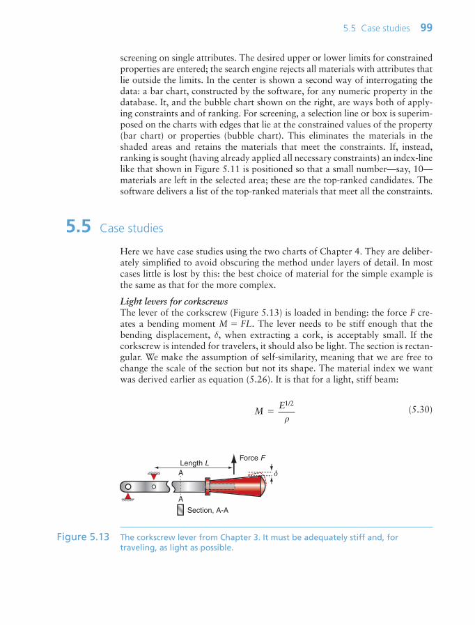
screening on single attributes. The desired upper or lower limits for constrainedproperties are entered; the search engine rejects all materials with attributes thatlie outside the limits. In the center is shown a second way of interrogating thedata: a bar chart, constructed by the software, for any numeric property in thedatabase. It, and the bubble chart shown on the right, are ways both of apply-ing constraints and of ranking. For screening, a selection line or box is superim-posed on the charts with edges that lie at the constrained values of the property(bar chart) or properties (bubble chart). This eliminates the materials in theshaded areas and retains the materials that meet the constraints. If, instead,ranking is sought (having already applied all necessary constraints) an index-linelike that shown in Figure 5.11 is positioned so that a small number—say, 10—materials are left in the selected area; these are the top-ranked candidates. Thesoftware delivers a list of the top-ranked materials that meet all the constraints.
5.5 Case studies
Here we have case studies using the two charts of Chapter 4. They are deliber-ately simplified to avoid obscuring the method under layers of detail. In mostcases little is lost by this: the best choice of material for the simple example isthe same as that for the more complex.
Light levers for corkscrewsThe lever of the corkscrew (Figure 5.13) is loaded in bending: the force F cre-ates a bending moment M FL. The lever needs to be stiff enough that thebending displacement, δ, when extracting a cork, is acceptably small. If thecorkscrew is intended for travelers, it should also be light. The section is rectan-gular. We make the assumption of self-similarity, meaning that we are free tochange the scale of the section but not its shape. The material index we wantwas derived earlier as equation (5.26). It is that for a light, stiff beam:
(5.30)ME
1/2
ρ
5.5 Case studies 99
Force F
δ
Section, A-A
A
A
Length L
Figure 5.13 The corkscrew lever from Chapter 3. It must be adequately stiff and, fortraveling, as light as possible.
Ch05-H8391 1/17/07 10:45 AM Page 99
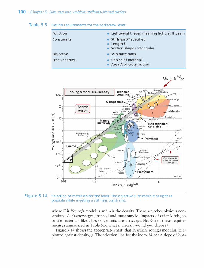
where E is Young’s modulus and ρ is the density. There are other obvious con-straints. Corkscrews get dropped and must survive impacts of other kinds, sobrittle materials like glass or ceramic are unacceptable. Given these require-ments, summarized in Table 5.5, what materials would you choose?
Figure 5.14 shows the appropriate chart: that in which Young’s modulus, E, isplotted against density, ρ. The selection line for the index M has a slope of 2, as
100 Chapter 5 Flex, sag and wobble: stiffness-limited design
Function • Lightweight lever, meaning light, stiff beam
Constraints • Stiffness S* specified• Length L• Section shape rectangular
Objective • Minimize mass
Free variables • Choice of material• Area A of cross-section
Table 5.5 Design requirements for the corkscrew lever
Density, ρ (Mg/m3)0.01
You
ng’s
mod
ulus
, E (
GP
a)
10−4
0.1 1 10
10−3
10−2
10−1
1
10
100
1000
Polyester
Foams
Polymers
Metals
Technicalceramics
Composites
Natural materials
Lead alloys
W alloys
SteelsTi alloys
Mg alloys
CFRP
GFRP
Al alloys
Rigid polymer foams
Flexible polymer foams
Ni alloys
Cu alloys
Zinc alloysPAPEEK
PMMA
PC
PET
Cork
Wood
Butyl rubber
Silicone elastomers
Concrete
WC
Al2O3SiC
Si3N4Young’s modulus–Density
B4C
EpoxiesPS
PTFE
EVA
NeopreneIsoprene
Polyurethane
Leather
MFA, 07
PP
PE
Glass
grain
grainT
Elastomers
Wood
Non-technicalceramics
Polyeo
ss Ni a
PSWo
Searchregion
Mb E1/2/ρ
E1/3
ρ
E1/2
ρ
Eρ
Guidelines for minimum mass
design2
∼∼
Figure 5.14 Selection of materials for the lever. The objective is to make it as light aspossible while meeting a stiffness constraint.
Ch05-H8391 1/17/07 10:45 AM Page 100

explained in Section 5.3; it is positioned so that a small group of materials is leftabove it. They are the materials with the largest values of M, and it is these thatare the best choice, provided they satisfy the other constraints. Three classes ofmaterials lie above the line: woods, carbon-fiber reinforced polymers (CFRPs)and a number of ceramics. Ceramics are brittle and expensive, ruling them out.The recommendation is clear. Make your the lever out of wood or—better—outof CFRP.
Cost: structural materials for buildingsThe most expensive thing that most people ever buy is the house they live in.Roughly half the cost of a house is the cost of the materials of which it is made,and these are used in large quantities (family house: around 200 tonnes; largeapartment block: around 20 000 tonnes). The materials are used in three ways:structurally to hold the building up; as cladding, to keep the weather out; andas ‘internals’, to insulate against heat and sound, and to provide comfort anddecoration.
Consider the selection of materials for the structure (Figure 5.15). They mustbe stiff, strong and cheap. Stiff, so that the building does not flex too muchunder wind loads or internal loading. Strong, so that there is no risk of it col-lapsing. And cheap, because such a lot of material is used. The structural frameof a building is rarely exposed to the environment, and is not, in general, vis-ible, so criteria of corrosion resistance or appearance are not important here.The design goal is simple: stiffness and strength at minimum cost. To be morespecific: consider the selection of material for floor joists, focusing on stiffness.Table 5.6 summarizes the requirements.
5.5 Case studies 101
Floorjoists
Figure 5.15 The materials of a building are chosen to perform three different roles. Thosefor the structure are chosen to carry loads. Those for the cladding provideprotection from the environment. Those for the interior control heat, light andsound. Here we explore structural materials.
Ch05-H8391 1/17/07 10:45 AM Page 101
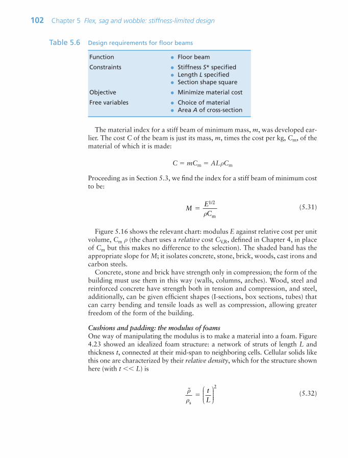
The material index for a stiff beam of minimum mass, m, was developed ear-lier. The cost C of the beam is just its mass, m, times the cost per kg, Cm, of thematerial of which it is made:
C mCm ALρCm
Proceeding as in Section 5.3, we find the index for a stiff beam of minimum costto be:
(5.31)
Figure 5.16 shows the relevant chart: modulus E against relative cost per unitvolume, Cm ρ (the chart uses a relative cost CV,R, defined in Chapter 4, in placeof Cm but this makes no difference to the selection). The shaded band has theappropriate slope for M; it isolates concrete, stone, brick, woods, cast irons andcarbon steels.
Concrete, stone and brick have strength only in compression; the form of thebuilding must use them in this way (walls, columns, arches). Wood, steel andreinforced concrete have strength both in tension and compression, and steel,additionally, can be given efficient shapes (I-sections, box sections, tubes) thatcan carry bending and tensile loads as well as compression, allowing greaterfreedom of the form of the building.
Cushions and padding: the modulus of foamsOne way of manipulating the modulus is to make a material into a foam. Figure4.23 showed an idealized foam structure: a network of struts of length L andthickness t, connected at their mid-span to neighboring cells. Cellular solids likethis one are characterized by their relative density, which for the structure shownhere (with t L) is
(5.32)ρρs
2
tL
⎛
⎝⎜⎜⎜
⎞
⎠⎟⎟⎟⎟
MEC
1/2
mρ
102 Chapter 5 Flex, sag and wobble: stiffness-limited design
Function • Floor beam
Constraints • Stiffness S* specified• Length L specified• Section shape square
Objective • Minimize material cost
Free variables • Choice of material• Area A of cross-section
Table 5.6 Design requirements for floor beams
Ch05-H8391 1/17/07 10:45 AM Page 102
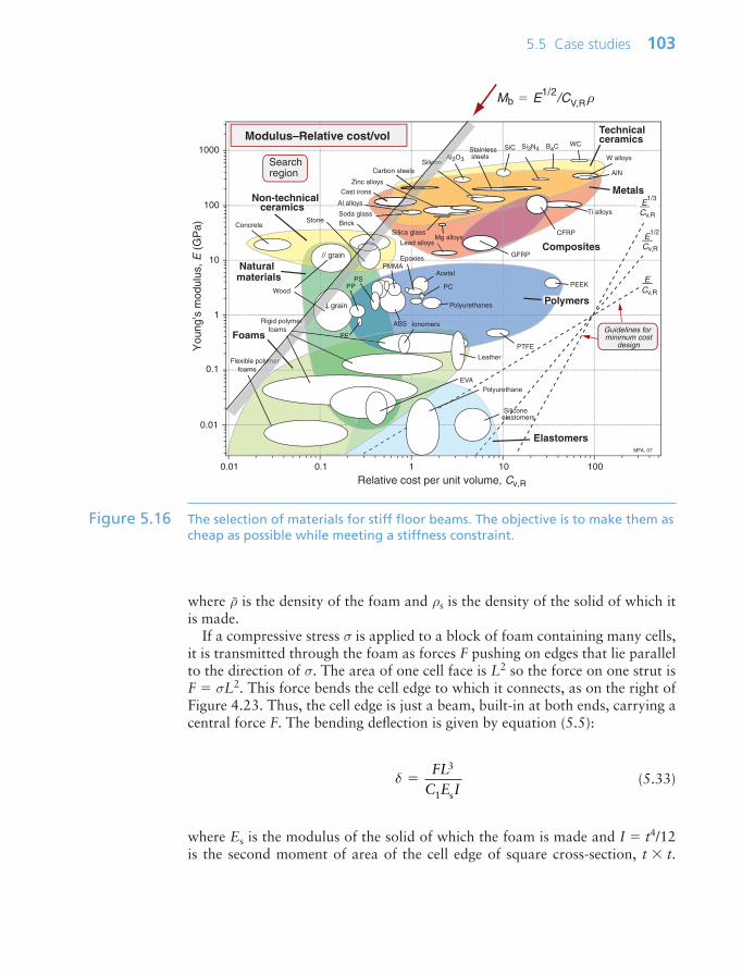
where ρ~ is the density of the foam and ρs is the density of the solid of which itis made.
If a compressive stress σ is applied to a block of foam containing many cells,it is transmitted through the foam as forces F pushing on edges that lie parallelto the direction of σ. The area of one cell face is L2 so the force on one strut isF σL2. This force bends the cell edge to which it connects, as on the right ofFigure 4.23. Thus, the cell edge is just a beam, built-in at both ends, carrying acentral force F. The bending deflection is given by equation (5.5):
(5.33)
where Es is the modulus of the solid of which the foam is made and I t4/12is the second moment of area of the cell edge of square cross-section, t t.
δ FL
C E I
3
1 s
5.5 Case studies 103
Relative cost per unit volume, Cv,R
You
ng’s
mod
ulus
, E (
GP
a)
0.01 0.1 1 10 100
0.01
0.1
1
10
100
1000
E1/3
Cv,R
E1/2
Cv,R
ECv,R
Guidelines for minimum cost
designFoams
Polymers
Metals
Technicalceramics
Composites
Natural materials
Lead alloys
W alloys
Carbon steels
Ti alloys
Mg alloysCFRP
GFRP
Al alloys
Rigid polymer foams
Flexible polymer foams
Zinc alloys
PS
PTFE
PCWood
Silicone elastomers
Concrete
Al2O3
SiC Si3N4
Modulus–Relative cost/volB4C
PP
EVAPolyurethane
Leather
Non-technical ceramics
MFA, 07
Cast irons
WC
Soda glass
Silica glass
Silicon
Stone Brick
ABS
Epoxies
Ionomers
AlN
Stainless steels
PEEK
PE
PMMA
Polyurethanes
Acetal
// grain
grainT
Elastomers
ymer
er
Alcon
T
Mb E1/2/CV,R ρ
Searchregion
Figure 5.16 The selection of materials for stiff floor beams. The objective is to make them ascheap as possible while meeting a stiffness constraint.
Ch05-H8391 1/17/07 10:45 AM Page 103
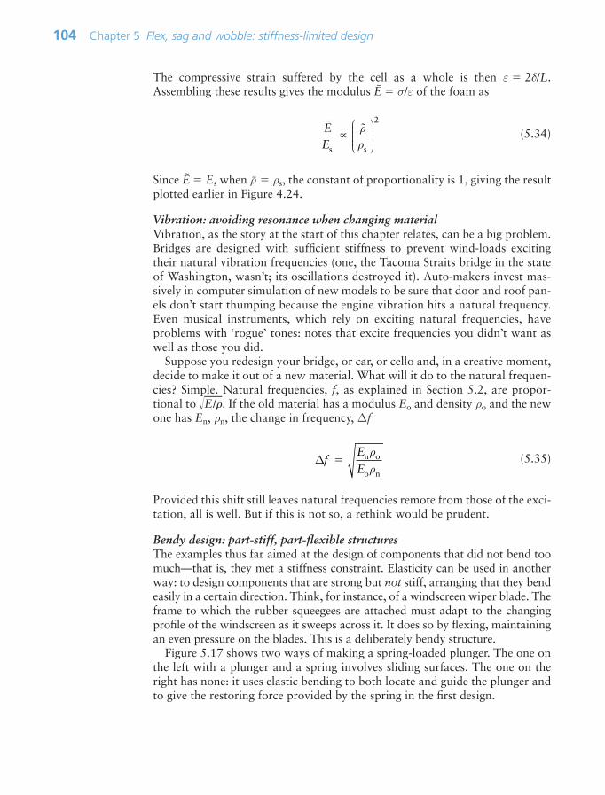
The compressive strain suffered by the cell as a whole is then ε 2δ/L.Assembling these results gives the modulus E
~ σ/ε of the foam as
(5.34)
Since E~
Es when ρ~ ρs, the constant of proportionality is 1, giving the resultplotted earlier in Figure 4.24.
Vibration: avoiding resonance when changing materialVibration, as the story at the start of this chapter relates, can be a big problem.Bridges are designed with sufficient stiffness to prevent wind-loads excitingtheir natural vibration frequencies (one, the Tacoma Straits bridge in the stateof Washington, wasn’t; its oscillations destroyed it). Auto-makers invest mas-sively in computer simulation of new models to be sure that door and roof pan-els don’t start thumping because the engine vibration hits a natural frequency.Even musical instruments, which rely on exciting natural frequencies, haveproblems with ‘rogue’ tones: notes that excite frequencies you didn’t want aswell as those you did.
Suppose you redesign your bridge, or car, or cello and, in a creative moment,decide to make it out of a new material. What will it do to the natural frequen-cies? Simple. Natural frequencies, f, as explained in Section 5.2, are propor-tional to E
—/–. If the old material has a modulus Eo and density ρo and the new
one has En, ρn, the change in frequency, ∆f
(5.35)
Provided this shift still leaves natural frequencies remote from those of the exci-tation, all is well. But if this is not so, a rethink would be prudent.
Bendy design: part-stiff, part-flexible structuresThe examples thus far aimed at the design of components that did not bend toomuch—that is, they met a stiffness constraint. Elasticity can be used in anotherway: to design components that are strong but not stiff, arranging that they bendeasily in a certain direction. Think, for instance, of a windscreen wiper blade. Theframe to which the rubber squeegees are attached must adapt to the changingprofile of the windscreen as it sweeps across it. It does so by flexing, maintainingan even pressure on the blades. This is a deliberately bendy structure.
Figure 5.17 shows two ways of making a spring-loaded plunger. The one onthe left with a plunger and a spring involves sliding surfaces. The one on theright has none: it uses elastic bending to both locate and guide the plunger andto give the restoring force provided by the spring in the first design.
∆fE
E n o
o n
ρρ
EEs s
2
ρρ
⎛
⎝⎜⎜⎜⎜
⎞
⎠⎟⎟⎟⎟⎟
104 Chapter 5 Flex, sag and wobble: stiffness-limited design
Ch05-H8391 1/17/07 10:45 AM Page 104
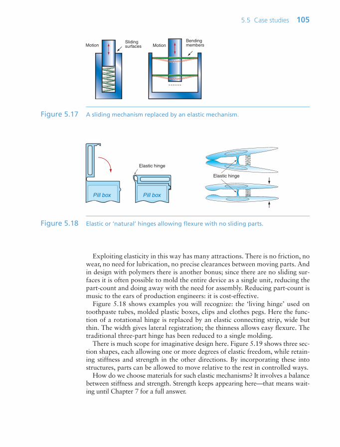
Exploiting elasticity in this way has many attractions. There is no friction, nowear, no need for lubrication, no precise clearances between moving parts. Andin design with polymers there is another bonus; since there are no sliding sur-faces it is often possible to mold the entire device as a single unit, reducing thepart-count and doing away with the need for assembly. Reducing part-count ismusic to the ears of production engineers: it is cost-effective.
Figure 5.18 shows examples you will recognize: the ‘living hinge’ used ontoothpaste tubes, molded plastic boxes, clips and clothes pegs. Here the func-tion of a rotational hinge is replaced by an elastic connecting strip, wide butthin. The width gives lateral registration; the thinness allows easy flexure. Thetraditional three-part hinge has been reduced to a single molding.
There is much scope for imaginative design here. Figure 5.19 shows three sec-tion shapes, each allowing one or more degrees of elastic freedom, while retain-ing stiffness and strength in the other directions. By incorporating these intostructures, parts can be allowed to move relative to the rest in controlled ways.
How do we choose materials for such elastic mechanisms? It involves a balancebetween stiffness and strength. Strength keeps appearing here—that means wait-ing until Chapter 7 for a full answer.
5.5 Case studies 105
Sliding surfacesMotion
Bending membersMotion
Figure 5.17 A sliding mechanism replaced by an elastic mechanism.
Elastic hinge
Pill boxPill box
Elastic hinge
Figure 5.18 Elastic or ‘natural’ hinges allowing flexure with no sliding parts.
Ch05-H8391 1/17/07 10:45 AM Page 105
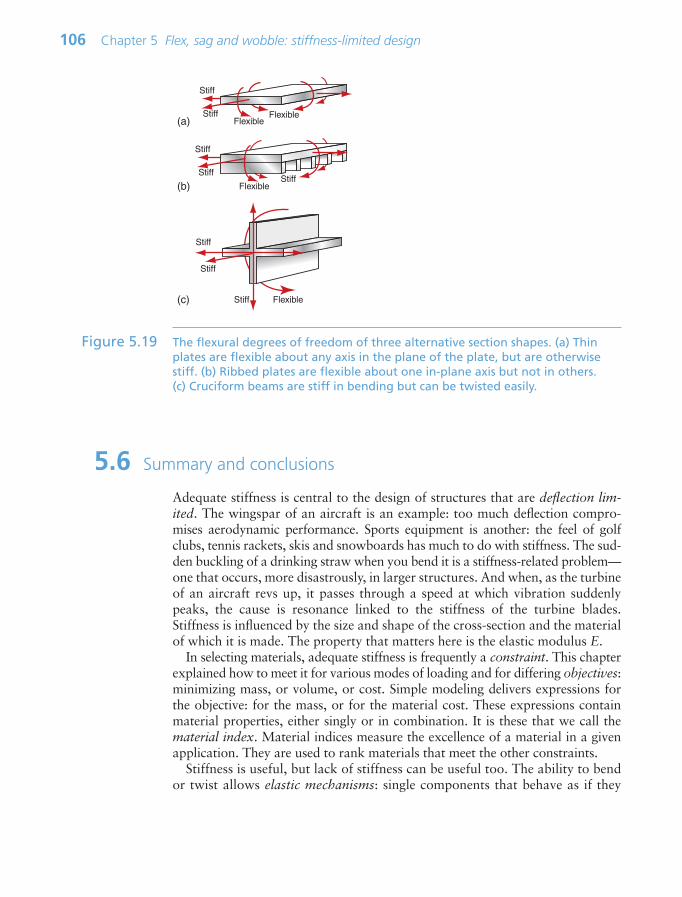
5.6 Summary and conclusions
Adequate stiffness is central to the design of structures that are deflection lim-ited. The wingspar of an aircraft is an example: too much deflection compro-mises aerodynamic performance. Sports equipment is another: the feel of golfclubs, tennis rackets, skis and snowboards has much to do with stiffness. The sud-den buckling of a drinking straw when you bend it is a stiffness-related problem—one that occurs, more disastrously, in larger structures. And when, as the turbineof an aircraft revs up, it passes through a speed at which vibration suddenlypeaks, the cause is resonance linked to the stiffness of the turbine blades.Stiffness is influenced by the size and shape of the cross-section and the materialof which it is made. The property that matters here is the elastic modulus E.
In selecting materials, adequate stiffness is frequently a constraint. This chapterexplained how to meet it for various modes of loading and for differing objectives:minimizing mass, or volume, or cost. Simple modeling delivers expressions forthe objective: for the mass, or for the material cost. These expressions containmaterial properties, either singly or in combination. It is these that we call thematerial index. Material indices measure the excellence of a material in a givenapplication. They are used to rank materials that meet the other constraints.
Stiffness is useful, but lack of stiffness can be useful too. The ability to bendor twist allows elastic mechanisms: single components that behave as if they
106 Chapter 5 Flex, sag and wobble: stiffness-limited design
Stiff
Stiff
Stiff
Flexible
Stiff
StiffFlexible
Flexible
StiffFlexible
Stiff
Stiff
(a)
(b)
(c)
Figure 5.19 The flexural degrees of freedom of three alternative section shapes. (a) Thinplates are flexible about any axis in the plane of the plate, but are otherwisestiff. (b) Ribbed plates are flexible about one in-plane axis but not in others. (c) Cruciform beams are stiff in bending but can be twisted easily.
Ch05-H8391 1/17/07 10:45 AM Page 106

had moving parts with bearings. Elastic mechanisms have limitations, but—where practical—they require no assembly, they have no maintenance require-ments and they are cheap.
The chapter ended by illustrating how indices are plotted onto material prop-erty charts to find the best selection. The method is a general one that we applyin later chapters to strength thermal, electrical, magnetic and optical properties.
5.7 Further reading
Ashby, M.F. (2005) Materials Selection in Mechanical Design, 3rd edition, Butterworth-Heinemann, Oxford, UK, Chapter 4. ISBN 0-7506-6168-2. (A more advanced textthat develops the ideas presented here, including a much fuller discussion of shapefactors and an expanded catalog of simple solutions to standard problems.)
Gere, J.M. (2006) Mechanics of Materials, 6th edition, Thompson Publishing, Toronto,Canada. ISBN 0-534-41793-0. (An intermediate level text on statics of structures byone of the fathers of the field; his books with Timoshenko introduced an entire gen-eration to the subject.)
Hosford, W.F. (2005) Mechanical Behavior of Materials, Cambridge University Press,Cambridge, UK. ISBN 0-521-84670-6. (A text that nicely links stress–strain behaviorto the micromechanics of materials.)
Jenkins, C.H.M. and Khanna, S.K. (2006) Mechanics of Materials, Elsevier Academic,Boston, MA, USA. ISBN 0-12-383852-5. (A simple introduction to mechanics,emphasizing design.)
Riley, W.F., Sturges, L.D. and Morris, D.H. (2003) Statics and Mechanics of Materials,2nd edition, McGraw-Hill, Hoboken, NJ, USA. ISBN 0-471-43446-9. (An intermedi-ate level text on the stress, strain and the relationships between them for many modesof loading. No discussion of micromechanics—response of materials to stress at themicroscopic level.)
Vable, M. (2002) Mechanics of Materials, Oxford University Press, Oxford, UK. ISBN0-19-513337-4. (An introduction to stress–strain relations, but without discussion ofthe micromechanics of materials.)
Young W.C. (1989) Roark’s Formulas for Stress and Strain, 6th edition, McGraw-Hill,New York, USA. ISBN 0-07-100373-8. (This is the ‘Yellow Pages’ of formulae forelastic problems—if the solution is not here, it doesn’t exist.)
5.8 Exercises
5.8 Exercises 107
Exercise E5.1 Distinguish between tension, torsion, bending and buckling.
Exercise E5.2 What is meant by a material index?
Exercise E5.3 Plot the index for a light, stiff panel on a copy of the modulus–density chart,positioning the line such that six materials are left above it. What classes dothey belong to?
Ch05-H8391 1/17/07 10:45 AM Page 107

108 Chapter 5 Flex, sag and wobble: stiffness-limited design
Exercise E5.4 The objective in selecting a material for a panel of given in-plane dimensionsfor the casing of a portable computer is that of minimizing the panel thick-ness h while meeting a constraint on bending stiffness, S*. What is the appro-priate material index?
Exercise E5.5 Derive the material index for a torsion bar with a solid circular section. Thelength L and the stiffness S* are specified, and the torsion bar is to be as lightas possible. Follow the steps used in the text for the beam, but replace thebending stiffness S* F/δ by the torsional stiffness S* T/(/L) (equation(5.8)), using the expression for K given in Figure 5.2.
Exercise E5.6 The speed of longitudinal waves in a material is proportional to E—
/–. Plot
contours of this quantity onto a copy of an E–ρ chart allowing you to readoff approximate values for any material on the chart. Which metals haveabout the same sound velocity as steel? Does sound move faster in titaniumor glass?
Exercise E5.7 A material is required for a cheap column with a solid circular cross-section thatmust support a load Fcrit without buckling. It is to have a height L. Write downan equation for the material cost of the column in terms of its dimensions, theprice per kg of the material, Cm, and the material density ρ. The cross-sectionarea A is a free variable—eliminate it by using the constraint that the bucklingload must not be less than Fcrit (equation (5.9)). Hence read off the index forfinding the cheapest tie. Plot the index on a copy of the appropriate chart andidentify three possible candidates.
Exercise E5.8 Devise an elastic mechanism that, when compressed, shears in a direction at rightangles to the axis of compression.
Exercise E5.9 Universal joints usually have sliding bearings. Devise a universal joint thatcould be molded as a single elastic unit, using a polymer.
Ch05-H8391 1/17/07 10:45 AM Page 108

5.9 Exploring design with CES (use Level 2, Materials, throughout)
5.10 Exploring the science with CES Elements 109
Exercise E5.10 Use a ‘Limit’ stage to find materials with modulus E 180 GPa and priceCm 3 $/kg.
Exercise E5.11 Use a ‘Limit’ stage to find materials with modulus E 2 GPa, densityρ 1000 kg/m3 and Price 3/kg.
Exercise E5.12 Make a bar chart of modulus, E. Add a tree stage to limit the selection topolymers alone. Which three polymers have the highest modulus?
Exercise E5.13 Make a chart showing modulus E and density ρ. Apply a selection line of slope1, corresponding to the index E/ρ positioning the line such that six materialsare left above it. Which are they and what families do they belong to?
Exercise E5.14 A material is required for a tensile tie to link the front and back walls of abarn to stabilize both. It must meet a constraint on stiffness and be as cheapas possible. To be safe the material of the tie must have a fracture toughnessK1c 18 MPa.m1/2 (defined in Chapter 8). The relevant index is
Construct a chart of E plotted against Cmρ. Add the constraint of adequatefracture toughness, meaning K1c 18 MPa.m1/2, using a ‘Limit’ stage. Thenplot an appropriate selection line on the chart and report the three materialsthat are the best choices for the tie.
ME
Cm
ρ
5.10 Exploring the science with CES Elements
Exercise E5.15 There is nothing that we can do to change the modulus or the density of thebuilding blocks of all materials: the elements. We have to live with the ones wehave got. Make a chart of modulus E plotted against the atomic number An toexplore the modulus across the Periodic Table. (Use a linear scale for An. To doso, change the default log scale to linear by double-clicking on the axis name toreveal the axis-choice dialog box and choose ‘Linear’.) Which element has thehighest modulus? Which has the lowest?
Exercise E5.16 Repeat Exercise E5.15, exploring instead the density ρ. Which solid elementhas the lowest density? Which has the highest?
Exercise E5.17 Make a chart of the sound velocity (E/ρ)1/2, for the elements. To do so, constructthe quantity (E/ρ)1/2 on the y-axis using the ‘Advanced’ facility in the axis-choicedialog box, and plot it against atomic number An. Use a linear scale for An asexplained in Exercise E5.15. (Multiply E by 109 to give the velocity in m/s).
Ch05-H8391 1/17/07 10:45 AM Page 109

This page intentionally left blank

Chapter 6Beyond elasticity: plasticity,
yielding and ductility
Chapter contents
6.1 Introduction and synopsis 1126.2 Strength, plastic work and ductility: 112
definition and measurement6.3 The big picture: charts for yield strength 1166.4 Drilling down: the origins of strength
and ductility 1186.5 Manipulating strength 1276.6 Summary and conclusions 1356.7 Further reading 1366.8 Exercises 1376.9 Exploring design with CES 1386.10 Exploring the science with
CES Elements 138
Dislocations in the intermetallic compound, Ni3Al. (Image courtesy of C. Rentenberger and H.P.
Karnthaler, Institute of Materials Physics, University ofVienna, Austria.)
Ch06-H8391.qxd 1/16/07 5:48 PM Page 111

112 Chapter 6 Beyond elasticity: plasticity, yielding and ductility
6.1 Introduction and synopsis
The verb ‘to yield’ has two, seemingly contradictory, meanings. To yield underforce is to submit to it, to surrender. To yield a profit has a different, more com-fortable, connotation: to bear fruit, to be useful. The yield strength, when speak-ing of a material, is the stress beyond which it becomes plastic. The term is wellchosen: yield and the plasticity that follows can be profitable—it allows metalsto be shaped and it allows structures to tolerate impact and absorb energy. Butthe unplanned yield of the span of a bridge or of the wing-spar of an aircraft orof the forks of your bicycle spells disaster.
This chapter is about yield and plasticity. For that reason it is mainly (but notwholly) about metals: it is the plasticity of iron and steel that made them thestructural materials on which the Industrial Revolution was built, enabling theengineering achievements of the likes of Telford1 and Brunel2. The dominance ofmetals in engineering, even today, derives from their ability to be rolled, forged,drawn and stamped.
6.2 Strength, plastic work and ductility: definition and measurement
Yield properties and ductility are measured using the standard tensile tests intro-duced in Chapter 4, with the materials taken to failure. Figures 6.1–6.3 showthe types of stress–strain behavior observed in different material classes. Theyield strength σy (or elastic limit σel)—units: MPa or MN/m2—requires carefuldefinition. For metals, the onset of plasticity is not always distinct so we identifyσy with the 0.2% proof stress—that is, the stress at which the stress–strain curvefor axial loading deviates by a strain of 0.2% from the linear elastic line asshown in Figure 6.1. It is the same in tension and compression. When strainedbeyond the yield point, most metals work harden, causing the rising part of thecurve, until a maximum, the tensile strength, is reached. This is followed in ten-sion by non-uniform deformation (necking) and fracture.
For polymers, σy is identified as the stress at which the stress–strain curvebecomes markedly nonlinear: typically, a strain of 1% (Figure 6.2). The behavior
1 Thomas Telford (1757–1834), Scottish engineer, brilliant proponent of the suspensionbridge at a time when its safety was a matter of debate. Telford may himself have haddoubts—he was given to lengthy prayer on the days that the suspension chains werescheduled to take the weight of the bridge. Most of his bridges, however, still stand.
2 Isambard Kingdom Brunel (1806–1859), perhaps the greatest engineer of the IndustrialRevolution (circa 1760–1860) in terms of design ability, personality, power of executionand sheer willingness to take risks—the Great Eastern, for example, was five times largerthan any previous ship ever built. He took the view that ‘great things are not done bythose who simply count the cost’. Brunel was a short man and self-conscious about hisheight; he favored tall top hats to make himself look taller.
Ch06-H8391.qxd 1/16/07 5:48 PM Page 112
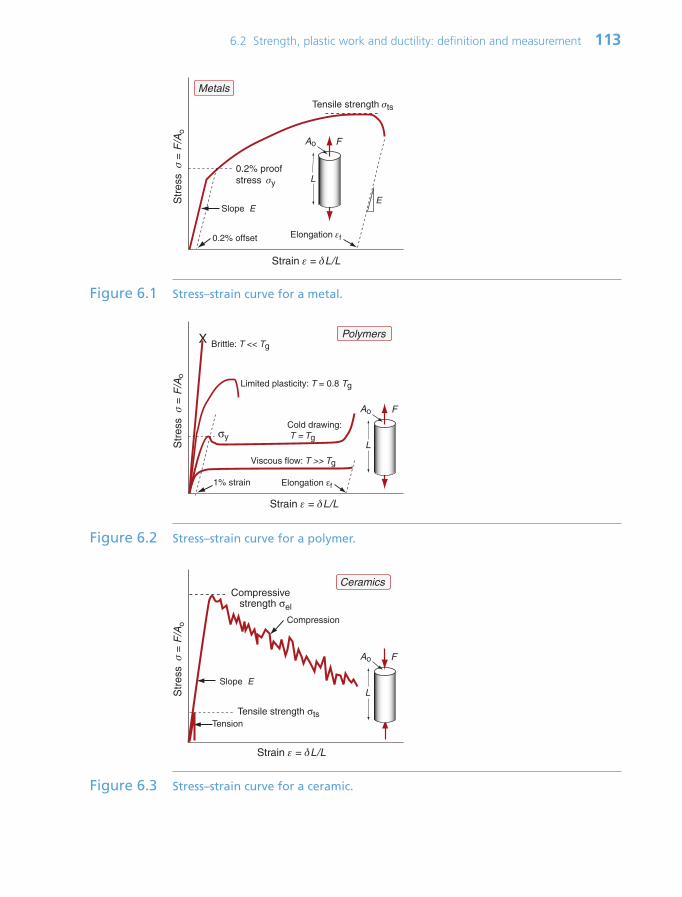
6.2 Strength, plastic work and ductility: definition and measurement 113
Str
ess
σ =
F/A
o
Strain ε = δL/L
Slope E
0.2% offset
FAo
L0.2% proof stress σy
Tensile strength σts
Metals
Elongation εf
E
Figure 6.1 Stress–strain curve for a metal.
Str
ess
σ =
F/A
o
Strain ε = δL/L
Brittle: T << Tg
Limited plasticity: T = 0.8 Tg
Cold drawing: T = Tg
Viscous flow: T >> Tg
1% strain
FAo
Lσy
PolymersX
Elongation εf
Figure 6.2 Stress–strain curve for a polymer.
Str
ess
σ =
F/A
o
Strain ε = δL/L
Slope E
Tension
Compression
FAo
L
Compressive strength σel
Tensile strength σts
Ceramics
Figure 6.3 Stress–strain curve for a ceramic.
Ch06-H8391.qxd 1/16/07 5:48 PM Page 113
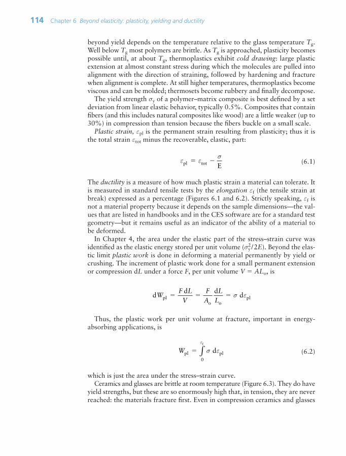
beyond yield depends on the temperature relative to the glass temperature Tg.Well below Tg most polymers are brittle. As Tg is approached, plasticity becomespossible until, at about Tg, thermoplastics exhibit cold drawing: large plasticextension at almost constant stress during which the molecules are pulled intoalignment with the direction of straining, followed by hardening and fracturewhen alignment is complete. At still higher temperatures, thermoplastics becomeviscous and can be molded; thermosets become rubbery and finally decompose.
The yield strength σy of a polymer–matrix composite is best defined by a setdeviation from linear elastic behavior, typically 0.5%. Composites that containfibers (and this includes natural composites like wood) are a little weaker (up to30%) in compression than tension because the fibers buckle on a small scale.
Plastic strain, εpl is the permanent strain resulting from plasticity; thus it isthe total strain εtot minus the recoverable, elastic, part:
(6.1)
The ductility is a measure of how much plastic strain a material can tolerate. Itis measured in standard tensile tests by the elongation εf (the tensile strain atbreak) expressed as a percentage (Figures 6.1 and 6.2). Strictly speaking, εf isnot a material property because it depends on the sample dimensions—the val-ues that are listed in handbooks and in the CES software are for a standard testgeometry—but it remains useful as an indicator of the ability of a material tobe deformed.
In Chapter 4, the area under the elastic part of the stress–strain curve wasidentified as the elastic energy stored per unit volume (σy
2/2E). Beyond the elas-tic limit plastic work is done in deforming a material permanently by yield orcrushing. The increment of plastic work done for a small permanent extensionor compression dL under a force F, per unit volume V ALo, is
Thus, the plastic work per unit volume at fracture, important in energy-absorbing applications, is
(6.2)
which is just the area under the stress–strain curve.Ceramics and glasses are brittle at room temperature (Figure 6.3). They do have
yield strengths, but these are so enormously high that, in tension, they are neverreached: the materials fracture first. Even in compression ceramics and glasses
Wpl pl0
df
σ εε
∫
dd d
dplo o
plWF LV
FA
LL
σ ε
ε εσ
pl tot E
114 Chapter 6 Beyond elasticity: plasticity, yielding and ductility
Ch06-H8391.qxd 1/16/07 5:48 PM Page 114
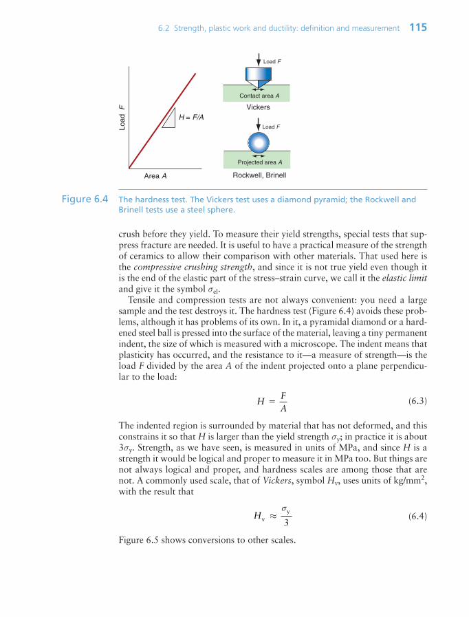
crush before they yield. To measure their yield strengths, special tests that sup-press fracture are needed. It is useful to have a practical measure of the strengthof ceramics to allow their comparison with other materials. That used here isthe compressive crushing strength, and since it is not true yield even though itis the end of the elastic part of the stress–strain curve, we call it the elastic limitand give it the symbol σel.
Tensile and compression tests are not always convenient: you need a largesample and the test destroys it. The hardness test (Figure 6.4) avoids these prob-lems, although it has problems of its own. In it, a pyramidal diamond or a hard-ened steel ball is pressed into the surface of the material, leaving a tiny permanentindent, the size of which is measured with a microscope. The indent means thatplasticity has occurred, and the resistance to it—a measure of strength—is theload F divided by the area A of the indent projected onto a plane perpendicu-lar to the load:
(6.3)
The indented region is surrounded by material that has not deformed, and thisconstrains it so that H is larger than the yield strength σy; in practice it is about3σy. Strength, as we have seen, is measured in units of MPa, and since H is astrength it would be logical and proper to measure it in MPa too. But things arenot always logical and proper, and hardness scales are among those that arenot. A commonly used scale, that of Vickers, symbol Hv, uses units of kg/mm2,with the result that
(6.4)
Figure 6.5 shows conversions to other scales.
Hvy
3≈
σ
HFA
6.2 Strength, plastic work and ductility: definition and measurement 115
Load
F
Area A
H = F/A
Load F
Contact area A
Load F
Projected area A
Vickers
Rockwell, Brinell
Figure 6.4 The hardness test. The Vickers test uses a diamond pyramid; the Rockwell andBrinell tests use a steel sphere.
Ch06-H8391.qxd 1/16/07 5:48 PM Page 115

The hardness test has the advantage of being non-destructive, so strength canbe measured without destroying the component, and it requires only a tiny vol-ume of material. But the information it provides is less accurate and less com-plete than the tensile test, so it is not used to provide critical design data.
6.3 The big picture: charts for yield strength
Strength can be displayed on material property charts. Two are particularlyuseful.
The strength–density chartFigure 6.6 shows the yield strength σy or elastic limit σel plotted against density ρ.The range of strength for engineering materials, like that of the modulus, spansabout six decades: from less than 0.01 MPa for foams, used in packaging andenergy-absorbing systems, to 104MPa for diamond, exploited in diamond tool-ing for machining and as the indenter of the Vickers hardness test. Members ofeach family again cluster together and can be enclosed in envelopes, each ofwhich occupies a characteristic part of the chart.
Comparison with the modulus–density chart (Figure 4.7) reveals some markeddifferences. The modulus of a solid is a well-defined quantity with a narrow rangeof values. The strength is not. The strength range for a given class of metals, suchas stainless steels, can span a factor of 10 or more, while the spread in stiffness
116 Chapter 6 Beyond elasticity: plasticity, yielding and ductility
Vickers
Brinell
Mohs
Rockwell A
Rockwell C
Approx. yieldstrength, MPa
100
200
300
400
500
600
700
800
900
12
3
4
5
6
7
8
9
100
200
300
400
500
600
700
800
900
1000
0
1600
1500
1400
1300
1200
1100
1800
1700
1900
2000
10203040
50
60
70
80
606570
75
80
85
90
500
1000
1500
2000
2500
3000
3500
0
5500
5000
4500
4000
6000
Figure 6.5 Common hardness scales compared with the yield strength.
Ch06-H8391.qxd 1/16/07 5:48 PM Page 116
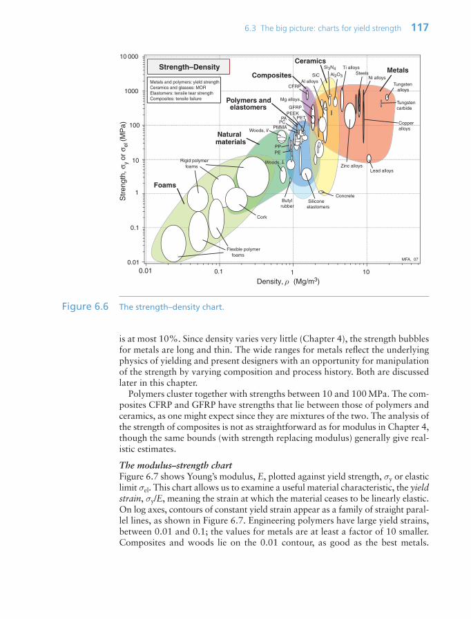
is at most 10%. Since density varies very little (Chapter 4), the strength bubblesfor metals are long and thin. The wide ranges for metals reflect the underlyingphysics of yielding and present designers with an opportunity for manipulationof the strength by varying composition and process history. Both are discussedlater in this chapter.
Polymers cluster together with strengths between 10 and 100 MPa. The com-posites CFRP and GFRP have strengths that lie between those of polymers andceramics, as one might expect since they are mixtures of the two. The analysis ofthe strength of composites is not as straightforward as for modulus in Chapter 4,though the same bounds (with strength replacing modulus) generally give real-istic estimates.
The modulus–strength chartFigure 6.7 shows Young’s modulus, E, plotted against yield strength, σy or elasticlimit σel. This chart allows us to examine a useful material characteristic, the yieldstrain, σy/E, meaning the strain at which the material ceases to be linearly elastic.On log axes, contours of constant yield strain appear as a family of straight paral-lel lines, as shown in Figure 6.7. Engineering polymers have large yield strains,between 0.01 and 0.1; the values for metals are at least a factor of 10 smaller.Composites and woods lie on the 0.01 contour, as good as the best metals.
6.3 The big picture: charts for yield strength 117
Density, ρ (Mg/m3)
0.01
Str
engt
h, σ
y or
σel
(MP
a)
0.01
100.1 1
0.1
1
10
100
1000
10 000
PPPE
Woods,
T
Foams
Polymers and elastomers
MetalsCeramics
Composites
Natural materials
Lead alloys
Tungsten alloys
SteelsTi alloys
Mg alloys
CFRP
GFRP
Al alloys
Rigid polymer foams
Flexible polymer foams
Ni alloys
Copper alloys
Zinc alloys
PAPEEK
PMMAPC
PET
Cork
Woods, ll
Butyl rubber
Silicone elastomers
Concrete
Tungstencarbide
Al2O3SiC
Si3N4Strength–Density
MFA, 07
Metals and polymers: yield strengthCeramics and glasses: MORElastomers: tensile tear strengthComposites: tensile failure
Figure 6.6 The strength–density chart.
Ch06-H8391.qxd 1/16/07 5:48 PM Page 117
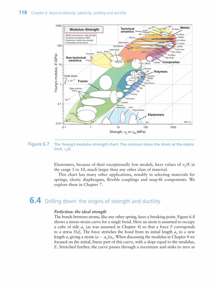
Elastomers, because of their exceptionally low moduli, have values of σy/E inthe range 1 to 10, much larger than any other class of material.
This chart has many other applications, notably in selecting materials forsprings, elastic diaphragms, flexible couplings and snap-fit components. Weexplore these in Chapter 7.
6.4 Drilling down: the origins of strength and ductility
Perfection: the ideal strengthThe bonds between atoms, like any other spring, have a breaking point. Figure 6.8shows a stress–strain curve for a single bond. Here an atom is assumed to occupya cube of side ao (as was assumed in Chapter 4) so that a force F corresponds to a stress F/a2
o. The force stretches the bond from its initial length ao to a newlength a, giving a strain (a ao)/ao. When discussing the modulus in Chapter 4 wefocused on the initial, linear part of this curve, with a slope equal to the modulus,E. Stretched further, the curve passes through a maximum and sinks to zero as
118 Chapter 6 Beyond elasticity: plasticity, yielding and ductility
Strength, σy or σel (MPa)
You
ng’s
mod
ulus
, E (
GP
a)
0.1 1 10 100 10000.01
0.1
1
10
100
1000
= 10 −4
Yield strainσy
10−3
10−210−1
Non-technical ceramics
MFA, 07
Foams
Polymers
MetalsTechnicalceramics
Composites
Lead alloys
W alloys
Ti alloys
Mg alloys
CFRP
GFRP
Al alloys
Rigid polymer foams
Ni alloys
Cu alloys
Zinc alloys
PMMA
Cork
Wood
Polyurethane
Silicone elastomers
Concrete
Al2O3
SiC
AlN
Modulus–StrengthB4C
EVA
Leather
Cast irons
WC
Soda glass
Silica glass
Silicon
Stone Brick
Epoxies
Ionomers
Steels
Polyurethane
PA
PC
PE
PTFE
PSPP
Phenolic
Metals and polymers: yield strengthCeramics and glasses: MORElastomers: tensile tear strengthComposites: tensile failure
Elastomers
101
E
Figure 6.7 The Young’s modulus–strength chart. The contours show the strain at the elasticlimit, σy/E.
Ch06-H8391.qxd 1/16/07 5:48 PM Page 118

the atoms lose communication. The peak is the bond strength—if you pullharder than this it will break. The same is true if you shear it rather than pullit.
The distance over which inter-atomic forces act is small—a bond is broken ifit is stretched to more than about 10% of its original length. So the forceneeded to break a bond is roughly:
(6.5)
where S, as before, is the bond stiffness. On this basis the ideal strength of asolid should therefore be roughly
(remembering that E So/ao, equation (4.17)).
or(6.6)
This doesn’t allow for the curvature of the force–distance curve; more refinedcalculations give a ratio of 1/15.
Figure 6.9 shows σy/E for metals, polymers and ceramics. None achieve theideal value of 1/10; most don’t even come close. Why not? It’s a familiar story:like most things in life, materials are imperfect.
Crystalline imperfection: defects in metals and ceramicsCrystals contain imperfections of several kinds. Figure 6.10 introduces thebroad families, distinguished by their dimensionality. At the top left are point
σideal 110E
≈
σidealmax
o2
o10 10≈
F
aSa
E
FS a
≈ o
10
6.4 Drilling down: the origins of strength and ductility 119
ao
a
F F
Strain
Equilibrium spacing, ao
Spacing atfailure, a*
Modulus E ao
ao
Str
ess
σ =
F/a
o2
a − aoao
0.2 0.3 0.40 0.1
Fmax/ao2
Figure 6.8 The stress–strain curve for a single atomic bond (it is assumed that each atomoccupies a cube of side aa).
Ch06-H8391.qxd 1/16/07 5:48 PM Page 119
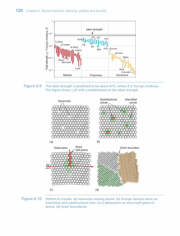
120 Chapter 6 Beyond elasticity: plasticity, yielding and ductility
Metals Polymers Ceramics
Yie
ld s
treng
th, σ
y / Y
oung
’s m
odul
us, E
10−4
10−3
1
10−2
10−1
Ideal strength
PTFE
PEPP
PS
PVC
PET
ABS
PA
Ti alloysLA steels
Lead
Copper
Al alloys
Mild steelBrass
Glass
Zirconia
Alumina
ConcreteBrick
Figure 6.9 The ideal strength is predicted to be about E/15, where E is Young’s modulus.The figure shows σy/E with a shaded band at the ideal strength.
Vacancies
(a)
Dislocation Extra half-plane
Slip
plane
(c)
Grain boundary
(d)
Substitutionalsolute
Interstitialsolute
(b)
Figure 6.10 Defects in crystals. (a) Vacancies–missing atoms. (b) Foreign (solute) atom oninterstitial and substitutional sites. (c) A dislocation–an extra half-plane ofatoms. (d) Grain boundaries.
Ch06-H8391.qxd 1/16/07 5:48 PM Page 120

defects. All crystals contain vacancies, shown in (a): sites at which an atom ismissing. They play a key role in diffusion, creep and sintering (Chapter 13), butwe don’t need them for the rest of this chapter because they do not influencestrength. The others do.
No crystal is totally, 100%, pure and perfect. Some impurities are inheritedfrom the process by which the material was made; more usually they are delib-erately added, creating alloys: a material in which a second (or third or fourth)element is dissolved. ‘Dissolved’ sounds like salt in water, but these are solidsolutions. Figure 6.10(b) shows both a substitutional solid solution (the dissolvedatoms replace those of the host) and an interstitial solid solution (the dissolvedatoms squeeze into the spaces or ‘interstices’ between the host atoms). The dis-solved atoms or solute rarely have the same size as those of the host material, sothey distort the surrounding lattice. The red atoms here are substitutional solute,some bigger and some smaller than those of the host; the cages of host atomsimmediately surrounding them, shown green, are distorted. If the solute atomsare particularly small, they don’t need to replace a host atom; instead, they dissolveinterstitially like the black atoms in the figure, again distorting the surroundinglattice. So solute causes local distortion; this distortion is one of the reasons thatalloys are stronger than pure materials, as we shall see in a moment.
Now to the key player, portrayed in Figure 6.10(c): the dislocation. ‘Dislocated’means ‘out of joint’ and this is not a bad description of what is happening here.The upper part of the crystal has one more double-layer of atoms than thelower part (the double-layer is needed to get the top-to-bottom registry right).It is dislocations that make metals soft and ductile. Dislocations distort thelattice—here the green atoms are the most distorted—and because of this theyhave elastic energy associated with them. If they cost energy, why are theythere? To grow a perfect crystal just one cubic centimeter in volume from a liq-uid or vapor, about 1023 atoms have to find their proper sites on the perfect lattice, and the chance of this happening is just too small. Even with the great-est care in assembling them, all crystals contain point defects, solute atoms anddislocations.
Most contain yet more drastic defects, among them grain boundaries. Figure6.10(d) shows such boundaries. Here three perfect, but differently oriented,crystals meet; the individual crystals are called grains, the meeting surfaces aregrain boundaries. In this sketch the atoms of the three crystals have been givendifferent colors to distinguish them, but here they are the same atoms. In realitygrain boundaries form in pure materials (when all the atoms are the same) andin alloys (when the mixture of atoms in one grain may differ in chemical com-position from those of the next).
Now put all this together. The seeming perfection of the steel of a precisionmachine tool or of the polished case of a gold watch is an illusion: they are rid-dled with defects. Imagine all of the frames of Figure 6.10 superimposed andyou begin to get the picture. Between them they explain diffusion, strength,ductility, electrical resistance, thermal conductivity and much more.
So defects in crystals are influential. For the rest of this section we focus ongetting to know just one of them: the dislocation.
6.4 Drilling down: the origins of strength and ductility 121
Ch06-H8391.qxd 1/16/07 5:48 PM Page 121
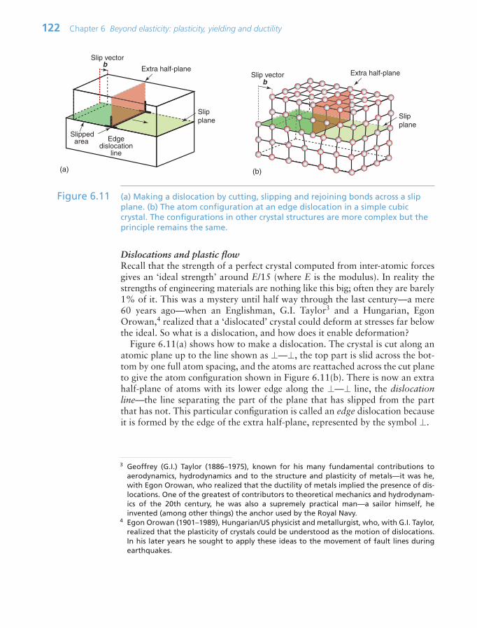
Dislocations and plastic flowRecall that the strength of a perfect crystal computed from inter-atomic forcesgives an ‘ideal strength’ around E/15 (where E is the modulus). In reality thestrengths of engineering materials are nothing like this big; often they are barely1% of it. This was a mystery until half way through the last century—a mere60 years ago—when an Englishman, G.I. Taylor3 and a Hungarian, EgonOrowan,4 realized that a ‘dislocated’ crystal could deform at stresses far belowthe ideal. So what is a dislocation, and how does it enable deformation?
Figure 6.11(a) shows how to make a dislocation. The crystal is cut along anatomic plane up to the line shown as ⊥—⊥, the top part is slid across the bot-tom by one full atom spacing, and the atoms are reattached across the cut planeto give the atom configuration shown in Figure 6.11(b). There is now an extrahalf-plane of atoms with its lower edge along the ⊥—⊥ line, the dislocationline—the line separating the part of the plane that has slipped from the partthat has not. This particular configuration is called an edge dislocation becauseit is formed by the edge of the extra half-plane, represented by the symbol ⊥.
122 Chapter 6 Beyond elasticity: plasticity, yielding and ductility
3 Geoffrey (G.I.) Taylor (1886–1975), known for his many fundamental contributions toaerodynamics, hydrodynamics and to the structure and plasticity of metals—it was he,with Egon Orowan, who realized that the ductility of metals implied the presence of dis-locations. One of the greatest of contributors to theoretical mechanics and hydrodynam-ics of the 20th century, he was also a supremely practical man—a sailor himself, heinvented (among other things) the anchor used by the Royal Navy.
4 Egon Orowan (1901–1989), Hungarian/US physicist and metallurgist, who, with G.I. Taylor,realized that the plasticity of crystals could be understood as the motion of dislocations. In his later years he sought to apply these ideas to the movement of fault lines during earthquakes.
Extra half-plane
Edgedislocation
line
Slipped area
bSlip vector
(a)
Slip plane
Extra half-planeb
Slip vector
(b)
Slip plane
Figure 6.11 (a) Making a dislocation by cutting, slipping and rejoining bonds across a slipplane. (b) The atom configuration at an edge dislocation in a simple cubiccrystal. The configurations in other crystal structures are more complex but theprinciple remains the same.
Ch06-H8391.qxd 1/16/07 5:48 PM Page 122
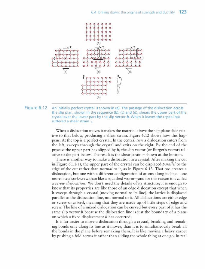
When a dislocation moves it makes the material above the slip plane slide rela-tive to that below, producing a shear strain. Figure 6.12 shows how this hap-pens. At the top is a perfect crystal. In the central row a dislocation enters fromthe left, sweeps through the crystal and exits on the right. By the end of theprocess the upper part has slipped by b, the slip vector (or Burger’s vector) rel-ative to the part below. The result is the shear strain γ shown at the bottom.
There is another way to make a dislocation in a crystal. After making the cutin Figure 6.11(a), the upper part of the crystal can be displaced parallel to theedge of the cut rather than normal to it, as in Figure 6.13. That too creates adislocation, but one with a different configuration of atoms along its line—onemore like a corkscrew than like a squashed worm—and for this reason it is calleda screw dislocation. We don’t need the details of its structure; it is enough toknow that its properties are like those of an edge dislocation except that whenit sweeps through a crystal (moving normal to its line), the lattice is displacedparallel to the dislocation line, not normal to it. All dislocations are either edgeor screw or mixed, meaning that they are made up of little steps of edge andscrew. The line of a mixed dislocation can be curved but every part of it has thesame slip vector b because the dislocation line is just the boundary of a planeon which a fixed displacement b has occurred.
It is far easier to move a dislocation through a crystal, breaking and remak-ing bonds only along its line as it moves, than it is to simultaneously break allthe bonds in the plane before remaking them. It is like moving a heavy carpetby pushing a fold across it rather than sliding the whole thing at one go. In real
6.4 Drilling down: the origins of strength and ductility 123
(a)
(b) (c) (d)
(e)
τ τ τ
b b
γ
Figure 6.12 An initially perfect crystal is shown in (a). The passage of the dislocation acrossthe slip plan, shown in the sequence (b), (c) and (d), shears the upper part of thecrystal over the lower part by the slip vector b. When it leaves the crystal hassuffered a shear strain γ.
Ch06-H8391.qxd 1/16/07 5:48 PM Page 123

crystals it is easier to make and move dislocations on some planes than onothers. The preferred planes are called slip planes and the preferred directionsof slip in these planes are called slip directions. A slip plane is shown in grayand a slip direction as an arrow on the fcc and bcc unit cells of Figure 4.11.
Slip displacements are tiny—one dislocation produces a displacement of about1010m. But if large numbers of dislocations traverse a crystal, moving on manydifferent planes, the shape of a material changes at the macroscopic length scale.Figure 6.14 shows just two dislocations traversing a sample loaded in tension.The slip steps (here very exaggerated) cause the sample to get a bit thinner andlonger. Repeating this millions of times on many planes gives the large plasticextensions observed in practice. Since none of this changes the average atomicspacing, the volume remains unchanged.
Why does a shear stress make a dislocation move?Crystals resist the motion of dislocations with a friction-like resistance f perunit length—we will examine its origins in a moment. For yielding to take placethe external stress must overcome the resistance f.
124 Chapter 6 Beyond elasticity: plasticity, yielding and ductility
S
S
Screw dislocation
line
Slipped area
Slip vector b
Slip plane
Figure 6.13 A screw dislocation. The slip vector b is parallel to the dislocation line S—S.
Figure 6.14 Dislocation motion causes extension
Ch06-H8391.qxd 1/16/07 5:48 PM Page 124

Imagine that one dislocation moves right across a slip plane, traveling thedistance L2, as in Figure 6.15. In doing so, it shifts the upper half of the crystalby a distance b relative to the lower half. The shear stress τ acts on an areaL1L2, giving a shear force Fs τ L1L2 on the surface of the block. If the dis-placement parallel to the block is b, the force does work
W τ L1L2 b (6.7)
This work is done against the resistance f per unit length, or f L1 on the lengthL1, and it does so over a displacement L2 (because the dislocation line movesthis far against f ), giving a total work against f of f L1L2. Equating this to thework W done by the applied stress τ gives
τ b f (6.8)
This result holds for any dislocation—edge, screw or mixed. So, provided theshear stress τ exceeds the value f/b it will make dislocations move and cause thecrystal to shear.
Line tension.The atoms near the core of a dislocation are displaced from their proper positions,as shown by green atoms back in Figure 6.10(c), and thus they have higher poten-tial energy. To keep the potential energy of the crystal as low as possible, thedislocation tries to be as short as possible—it behaves as if it had a line tension, T,like an elastic band. The tension can be calculated but it needs advanced elas-ticity theory to do it (the books listed under ‘Further reading’ give the analysis).We just need the answer. It is that the line tension, an energy per unit length(just as a surface tension is an energy per unit area), is
(6.9)T Eb≈12
2
6.4 Drilling down: the origins of strength and ductility 125
(a)
Slip plane
(b)
Dislocation line
Force τbper unit length
bSlip vector
Resistance fper unit length
Shearstress τ
L1L2
Force τbper unit length
Resistance fper unit length
Dislocation line
Slipped area of plane
L2
L1
Figure 6.15 The force on a dislocation. (a) Perspective view. (b) Plan view of slip plane.
Ch06-H8391.qxd 1/16/07 5:48 PM Page 125
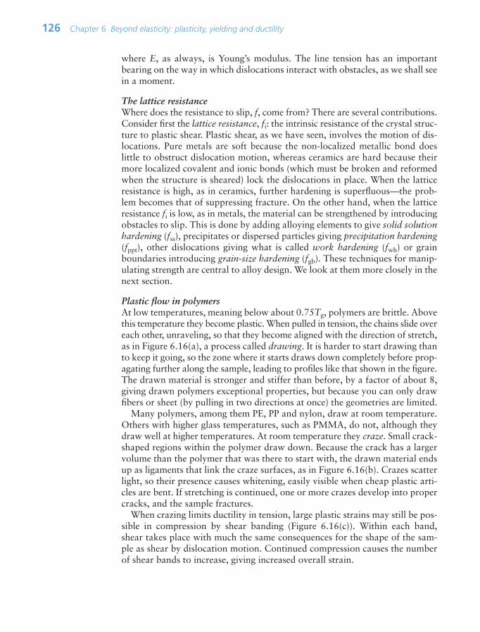
where E, as always, is Young’s modulus. The line tension has an importantbearing on the way in which dislocations interact with obstacles, as we shall seein a moment.
The lattice resistanceWhere does the resistance to slip, f, come from? There are several contributions.Consider first the lattice resistance, fi: the intrinsic resistance of the crystal struc-ture to plastic shear. Plastic shear, as we have seen, involves the motion of dis-locations. Pure metals are soft because the non-localized metallic bond doeslittle to obstruct dislocation motion, whereas ceramics are hard because theirmore localized covalent and ionic bonds (which must be broken and reformedwhen the structure is sheared) lock the dislocations in place. When the latticeresistance is high, as in ceramics, further hardening is superfluous—the prob-lem becomes that of suppressing fracture. On the other hand, when the latticeresistance fi is low, as in metals, the material can be strengthened by introducingobstacles to slip. This is done by adding alloying elements to give solid solutionhardening (fss), precipitates or dispersed particles giving precipitation hardening(fppt), other dislocations giving what is called work hardening (fwh) or grainboundaries introducing grain-size hardening (fgb). These techniques for manip-ulating strength are central to alloy design. We look at them more closely in thenext section.
Plastic flow in polymersAt low temperatures, meaning below about 0.75Tg, polymers are brittle. Abovethis temperature they become plastic. When pulled in tension, the chains slide overeach other, unraveling, so that they become aligned with the direction of stretch,as in Figure 6.16(a), a process called drawing. It is harder to start drawing thanto keep it going, so the zone where it starts draws down completely before prop-agating further along the sample, leading to profiles like that shown in the figure.The drawn material is stronger and stiffer than before, by a factor of about 8,giving drawn polymers exceptional properties, but because you can only drawfibers or sheet (by pulling in two directions at once) the geometries are limited.
Many polymers, among them PE, PP and nylon, draw at room temperature.Others with higher glass temperatures, such as PMMA, do not, although theydraw well at higher temperatures. At room temperature they craze. Small crack-shaped regions within the polymer draw down. Because the crack has a largervolume than the polymer that was there to start with, the drawn material endsup as ligaments that link the craze surfaces, as in Figure 6.16(b). Crazes scatterlight, so their presence causes whitening, easily visible when cheap plastic arti-cles are bent. If stretching is continued, one or more crazes develop into propercracks, and the sample fractures.
When crazing limits ductility in tension, large plastic strains may still be pos-sible in compression by shear banding (Figure 6.16(c)). Within each band,shear takes place with much the same consequences for the shape of the sam-ple as shear by dislocation motion. Continued compression causes the numberof shear bands to increase, giving increased overall strain.
126 Chapter 6 Beyond elasticity: plasticity, yielding and ductility
Ch06-H8391.qxd 1/16/07 5:48 PM Page 126
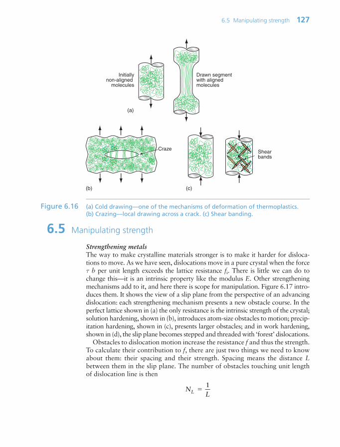
6.5 Manipulating strength
Strengthening metalsThe way to make crystalline materials stronger is to make it harder for disloca-tions to move. As we have seen, dislocations move in a pure crystal when the forceτ b per unit length exceeds the lattice resistance fi. There is little we can do tochange this—it is an intrinsic property like the modulus E. Other strengtheningmechanisms add to it, and here there is scope for manipulation. Figure 6.17 intro-duces them. It shows the view of a slip plane from the perspective of an advancingdislocation: each strengthening mechanism presents a new obstacle course. In theperfect lattice shown in (a) the only resistance is the intrinsic strength of the crystal;solution hardening, shown in (b), introduces atom-size obstacles to motion; precip-itation hardening, shown in (c), presents larger obstacles; and in work hardening,shown in (d), the slip plane becomes stepped and threaded with ‘forest’ dislocations.
Obstacles to dislocation motion increase the resistance f and thus the strength.To calculate their contribution to f, there are just two things we need to knowabout them: their spacing and their strength. Spacing means the distance Lbetween them in the slip plane. The number of obstacles touching unit lengthof dislocation line is then
NLL 1
6.5 Manipulating strength 127
Drawn segment with aligned molecules
Initiallynon-aligned
molecules
Shear bands
Craze
(a)
(b) (c)
Figure 6.16 (a) Cold drawing—one of the mechanisms of deformation of thermoplastics.(b) Crazing—local drawing across a crack. (c) Shear banding.
Ch06-H8391.qxd 1/16/07 5:48 PM Page 127
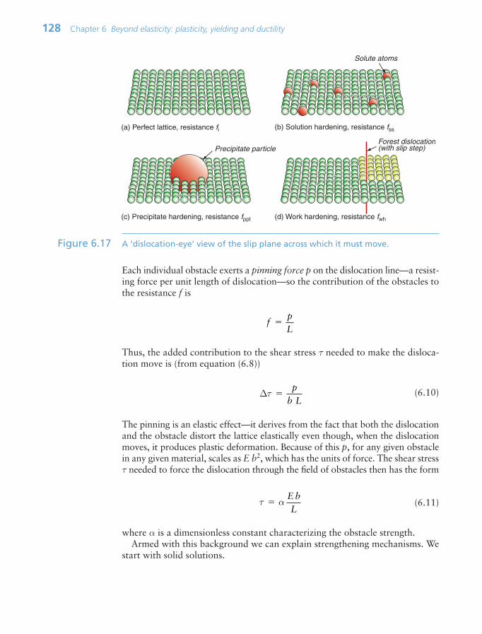
Each individual obstacle exerts a pinning force p on the dislocation line—a resist-ing force per unit length of dislocation—so the contribution of the obstacles tothe resistance f is
Thus, the added contribution to the shear stress τ needed to make the disloca-tion move is (from equation (6.8))
(6.10)
The pinning is an elastic effect—it derives from the fact that both the dislocationand the obstacle distort the lattice elastically even though, when the dislocationmoves, it produces plastic deformation. Because of this p, for any given obstaclein any given material, scales as E b2, which has the units of force. The shear stressτ needed to force the dislocation through the field of obstacles then has the form
(6.11)
where α is a dimensionless constant characterizing the obstacle strength.Armed with this background we can explain strengthening mechanisms. We
start with solid solutions.
τ αE bL
∆τ p
b L
fpL
128 Chapter 6 Beyond elasticity: plasticity, yielding and ductility
(a) Perfect lattice, resistance fi
Precipitate particle
(c) Precipitate hardening, resistance fppt
(b) Solution hardening, resistance fss
Solute atoms
Forest dislocation(with slip step)
(d) Work hardening, resistance fwh
Figure 6.17 A ‘dislocation-eye’ view of the slip plane across which it must move.
Ch06-H8391.qxd 1/16/07 5:48 PM Page 128
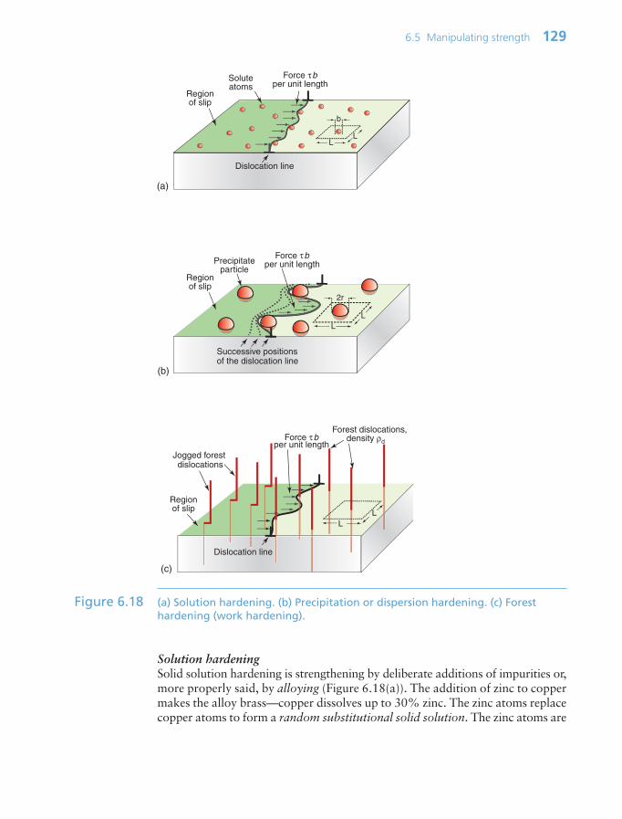
Solution hardeningSolid solution hardening is strengthening by deliberate additions of impurities or,more properly said, by alloying (Figure 6.18(a)). The addition of zinc to coppermakes the alloy brass—copper dissolves up to 30% zinc. The zinc atoms replacecopper atoms to form a random substitutional solid solution. The zinc atoms are
6.5 Manipulating strength 129
LL
b
Soluteatoms
Regionof slip
Dislocation line
Force τbper unit length
LL
2r
Precipitateparticle
Regionof slip
Successive positions of the dislocation line
Force τbper unit length
Force τbper unit length
LL
Forest dislocations,density ρd
Regionof slip
Dislocation line
Jogged forest dislocations
(a)
(b)
(c)
Figure 6.18 (a) Solution hardening. (b) Precipitation or dispersion hardening. (c) Foresthardening (work hardening).
Ch06-H8391.qxd 1/16/07 5:48 PM Page 129

bigger that those of copper and, in squeezing into the copper lattice, they distortit. This roughens the slip plane, so to speak, making it harder for dislocations tomove, thereby adding an additional resistance fss, opposing dislocation motion.The figure illustrates that the concentration of solute, expressed as an atomfraction, is on average:
where L is the spacing of obstacles in the slip plane and b is the atom size. Thus,
Plugging this into equation (6.11) relates the contribution of solid solution tothe shear stress required to move the dislocation:
τss α E c1/2 (6.12)
τss increases as the square root of the solute concentration. Brass, bronze andstainless steels, and many other metallic alloys, derive their strength in this way.They differ only in the extent to which the solute distorts the crystal, describedby the constant α.
Dispersion and precipitate strengtheningA more effective way to impede dislocations is to disperse small, strong part-icles in their path. One way to make such a microstructure is to disperse smallsolid particles of a high melting point compound into a liquid metal, and to cast itto shape, trapping the particles in place—it is the way that metal–matrix com-posites such as Al–SiC are made. An alternative is to form the particles in situ bya precipitation process. If a solute (copper, say) is dissolved in a metal (aluminum,for instance) at high temperature when both are molten, and the alloy is solidifiedand cooled to room temperature, the solute precipitates as small particles,much as salt will crystallize from a saturated solution when it is cooled. Analloy of aluminum containing 4% copper, treated in this way, gives very small,closely spaced precipitates of the hard compound CuAl2. Copper alloyed witha little beryllium, similarly treated, gives precipitates of the compound CuBe.Most steels are strengthened by precipitates of carbides, obtained in this way.The precipitates give a large contribution to f.
Figure 6.18(b) shows how particles obstruct dislocation motion. If the particlesare too strong for the dislocation to slice through them, the force τ b pushes thedislocation between them, bending it to a tighter and tighter radius against itsline tension (equation (6.9)). The radius is at a minimum when it reaches halfthe particle spacing, L; after that it can expand under lower stress. It is a bit likeblowing up a bicycle inner tube when the outer tire has a hole in it: once you reach
Lb
c
1/2
cbL
2
2
130 Chapter 6 Beyond elasticity: plasticity, yielding and ductility
Ch06-H8391.qxd 1/16/07 5:48 PM Page 130

the pressure that balloons the inner tube through the hole, the balloon needs asmaller pressure to get bigger still. The critical configuration is the semicircularone: here the total force τ b L on one segment of length L is just balanced by theforce 2T due to the line tension (equation (6.10)), acting on either side of thebulge, as in Figure 6.19. The dislocation escapes when
(6.13)
The obstacles thus exert a resistance of fppt 2T/L. Precipitation hardening isan effective way to increasing strength: precipitate-hardened aluminum alloyscan be 15 times stronger than pure aluminum.
Work hardeningThe rising part of the stress–strain curve of Figure 6.1 is caused by work harden-ing: it is caused by the accumulation of dislocations generated by plastic defor-mation. The dislocation density, ρd, is defined as the length of dislocation lineper unit volume (m/m3). Even in an annealed soft metal, the dislocation densityis around 1010m/m3, meaning that a 1 cm cube (the size of a cube of sugar) con-tains about 10 km of dislocation line. When metals are deformed, dislocationsmultiply, causing their density to grow to as much as 1017m/m3 or more—100million km per cubic centimeter. A moving dislocation now finds that its slipplane is penetrated by a forest of intersecting dislocations with an average spacingL ρd
1/2 (since ρd is a number per unit area). Figure 6.18(c) suggests the pic-ture. If a moving dislocation advances, it shears the material above the slip planerelative to that below, and that creates a little step called a jog in each forest dis-location. The jogs have potential energy—they are tiny segments of dislocation oflength b—with the result that each exerts a pinning force p E b2/2 on themoving dislocation. Assembling these results into equation (6.10) gives
(6.14)τ ρwh d2
≈E b
τppt2
T
b LE bL
≈
6.5 Manipulating strength 131
Force τbL
T
T
(a) (b) (c)
LRegionof slip
Regionof slip
Figure 6.19 Successive positions of a dislocation as it bypasses particles that obstruct its motion.The critical configuration is that with the tightest curvature, shown in (b).
Ch06-H8391.qxd 1/16/07 5:48 PM Page 131

The greater the density of dislocations, the smaller the spacing between them,and so the greater their contribution to τwh.
All metals work harden. It can be a nuisance: if you want to roll thin sheet,work hardening quickly raises the yield strength so much that you have to stopand anneal the metal (heat it up to remove the accumulated dislocations) beforeyou can go on—a trick known to blacksmiths for centuries. But it is also use-ful: it is a potent strengthening method, particularly for alloys that cannot beheat-treated to give precipitation hardening.
Grain boundary hardeningAlmost all metals are polycrystalline, made up of tiny, randomly oriented, crystals,or grains, meeting at grain boundaries like those of Figure 6.10(d). The grain size,D, is typically 10–100 µm. These boundaries obstruct dislocation motion. A dis-location in one grain—call it grain 1—can’t just slide into the next (grain 2)because the slip planes don’t line up. Instead, new dislocations have to nucleatein grain 2 with slip vectors that, if superimposed, match that of the dislocationin grain 1 so that the displacements match at the boundary. This gives anothercontribution to strength, τgb, that is found to scale as D1/2, giving
(6.15)
where kp is called the Petch constant, after the man who first measured it. Fornormal grain sizes τgb is small and not a significant source of strength, but formaterials that are microcrystalline (D 1 µm) or nanocrystalline (D approach-ing 1 nm) it becomes significant.
Relationship between dislocation strength and yield strengthTo a first approximation the strengthening mechanisms add up, giving a shearyield strength, τy, of
τy τi τss τppt τwh τgb (6.16)
Strong materials either have a high intrinsic strength, τi (like diamond), or theyrely on the superposition of solid solution strengthening τss, precipitates τppt andwork hardening τwh (like high-tensile steels). Nanocrystalline solids exploit, inaddition, the contribution of τgb.
Before we can use this information, one problem remains: we have calculatedthe yield strength of one crystal, loaded in shear. We want the yield strength ofa polycrystalline material in tension. To link them there are two simple steps.First, a uniform tensile stress σ creates a shear stress on planes that lie at an angleto the tensile axis; dislocations will first move on the slip plane on which thisshear stress is greatest. Figure 6.20 shows how this is calculated. A tensile force Facting on a rod of cross-section A, if resolved parallel to a plane with a normal
τgb k
D
p
132 Chapter 6 Beyond elasticity: plasticity, yielding and ductility
Ch06-H8391.qxd 1/16/07 5:48 PM Page 132

that lies at an angle θ to the axis of tension, gives a force F sin θ in the plane.The area of this plane is A/cos θ, so the shear stress is
where σ F/A is the tensile stress. The value of τ is plotted against θ in the fig-ure. The maximum lies at an angle of 45°, when τ σ/2.
Second, when this shear stress acts on an aggregate of crystals, some crystalswill have their slip planes oriented favorably with respect to the shear stress, otherswill not. This randomness of orientation jacks up the strength by a further fac-tor of 1.5 (called the Taylor factor — see the footnote on p. 122). Combiningthese results, the tensile stress to cause yielding of a sample that has manygrains is approximately three times the shear strength of a single crystal:
σy 3 τy
Thus, the superposition of strengthening mechanisms in equation (6.16) appliesequally to the yield strength, σy.
Strength and ductility of alloysOf all the properties that materials scientists and engineers have sought tomanipulate, the strength of metals and alloys is probably the most explored. Itis easy to see why—Table 6.1 gives a small selection of the applications of metalsand their alloys. Their importance in engineering design is enormous. The hard-ening mechanisms are often used in combination. This is illustrated graphically
τθθ
σ θ θ FA
sin/cos
sin cos
6.5 Manipulating strength 133
θ
F sin θ
F cos θF
Force F
F
Area A
cos θA
Area Shear
stress τ
Tensilestress σ
θ = 45οθ = 0ο
θ = 90ο
τ =
σ s
in θ
cos
θ
τ = σ/2
Angle θ0 9045
θ
Figure 6.20 The resolution of stress. A tensile stress σ gives a maximum shear stress τ σ/2on a plane at 45° to the tensile axis.
Ch06-H8391.qxd 1/16/07 5:48 PM Page 133
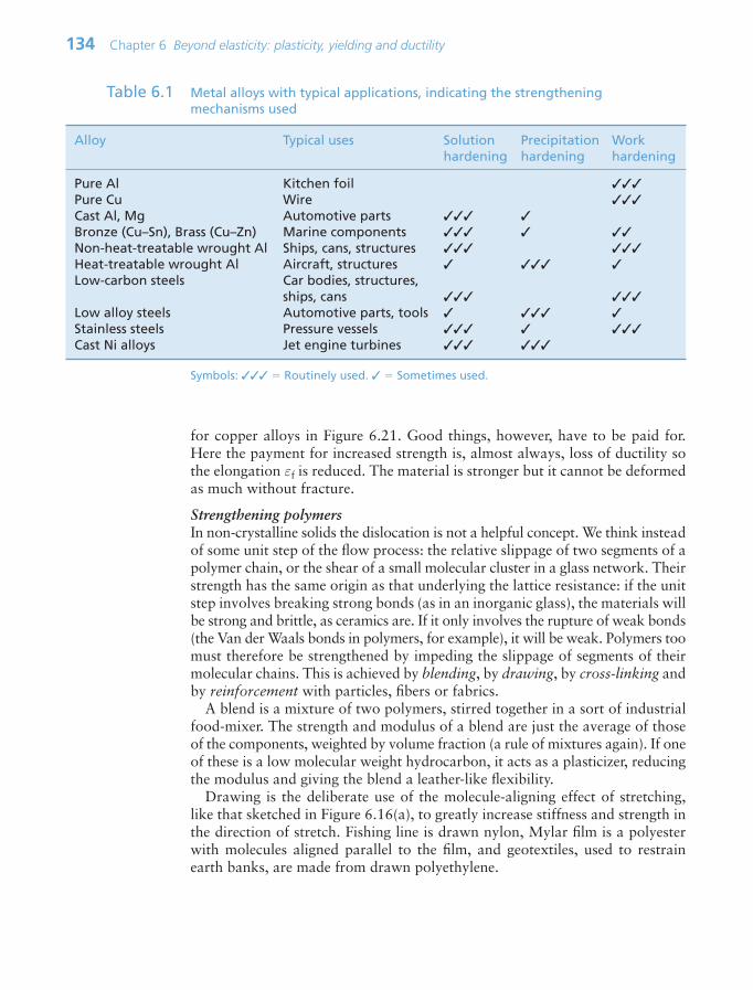
134 Chapter 6 Beyond elasticity: plasticity, yielding and ductility
Alloy Typical uses Solution Precipitation Workhardening hardening hardening
Pure Al Kitchen foil
Pure Cu Wire
Cast Al, Mg Automotive parts
Bronze (Cu–Sn), Brass (Cu–Zn) Marine components
Non-heat-treatable wrought Al Ships, cans, structures
Heat-treatable wrought Al Aircraft, structures
Low-carbon steels Car bodies, structures,ships, cans
Low alloy steels Automotive parts, tools
Stainless steels Pressure vessels
Cast Ni alloys Jet engine turbines
Table 6.1 Metal alloys with typical applications, indicating the strengthening mechanisms used
Symbols: Routinely used. Sometimes used.
for copper alloys in Figure 6.21. Good things, however, have to be paid for.Here the payment for increased strength is, almost always, loss of ductility sothe elongation εf is reduced. The material is stronger but it cannot be deformedas much without fracture.
Strengthening polymersIn non-crystalline solids the dislocation is not a helpful concept. We think insteadof some unit step of the flow process: the relative slippage of two segments of apolymer chain, or the shear of a small molecular cluster in a glass network. Theirstrength has the same origin as that underlying the lattice resistance: if the unitstep involves breaking strong bonds (as in an inorganic glass), the materials willbe strong and brittle, as ceramics are. If it only involves the rupture of weak bonds(the Van der Waals bonds in polymers, for example), it will be weak. Polymers toomust therefore be strengthened by impeding the slippage of segments of theirmolecular chains. This is achieved by blending, by drawing, by cross-linking andby reinforcement with particles, fibers or fabrics.
A blend is a mixture of two polymers, stirred together in a sort of industrialfood-mixer. The strength and modulus of a blend are just the average of thoseof the components, weighted by volume fraction (a rule of mixtures again). If oneof these is a low molecular weight hydrocarbon, it acts as a plasticizer, reducingthe modulus and giving the blend a leather-like flexibility.
Drawing is the deliberate use of the molecule-aligning effect of stretching,like that sketched in Figure 6.16(a), to greatly increase stiffness and strength inthe direction of stretch. Fishing line is drawn nylon, Mylar film is a polyesterwith molecules aligned parallel to the film, and geotextiles, used to restrainearth banks, are made from drawn polyethylene.
Ch06-H8391.qxd 1/16/07 5:48 PM Page 134

Cross-linking, sketched in Figures 4.18 and 4.19, creates strong bonds betweenmolecules that were previously linked by weak Van der Waals forces. Vulcanizedrubber is rubber that has been cross-linked, and the superior strength of epox-ies derives from cross-linking.
Reinforcement is possible with particles of cheap fillers—sand, talc or wooddust. Far more effective is reinforcement with fibers—usually glass or carbon—either continuous or chopped, as explained in Chapter 4.
6.6 Summary and conclusions
Load-bearing structures require materials with reliable, reproducible strength.There is more than one measure of strength. Elastic design requires that no partof the structure suffers plastic deformation, and this means that the stresses init must nowhere exceed the yield strength, σy, of ductile materials or the elasticlimit of those that are not ductile. Plastic design, by contrast, allows some partsof the structure to deform plastically so long as the structure as a whole doesnot collapse. Then two further properties become relevant: the ductility, εf,and the tensile strength, σts, which are the maximum strain and the maximumstress the material can tolerate before fracture. The tensile strength is generallylarger than the yield strength because of work hardening.
6.6 Summary and conclusions 135
1 10 10020
50
100
200
500
1000
2000
Yie
ld s
treng
th σ
y, te
nsio
n (M
Pa)
Elongation εf (%)
Pure, softcopper
Copper–beryllium alloys
Work hardening
Brass, work hardened
Brass, soft
Pure copper, work hardened
Solution hardening
Precipitation hardening
Figure 6.21 Strengthening mechanisms and the consequent drop in ductility, here shown forcopper alloys. The mechanisms are frequently combined. The greater thestrength, the lower the ductility (the elongation to fracture, εf).
Ch06-H8391.qxd 1/16/07 5:48 PM Page 135

Charts plotting strength, like those plotting modulus, show that materialfamilies occupy different areas of material property space, depending on thestrengthening mechanisms on which they rely. Crystal defects—particularlydislocations—are central to the understanding of these. It is the motion of dis-locations that gives plastic flow in crystalline solids, giving them unexpectedlylow strengths. When strength is needed it has to be provided by the strengthen-ing mechanism that impedes dislocation motion.
First among these is the lattice resistance—the intrinsic resistance of the crys-tal to dislocation motion. Others can be deliberately introduced by alloyingand heat treatment. Solid solution hardening, dispersion and precipitationhardening, work hardening and grain boundary hardening add to the latticeresistance. The strongest materials combine them all.
Non-crystalline solids—particularly polymers—deform in a less organizedway by the pulling of the tangled polymer chains into alignment with the direc-tion of deformation. This leads to cold drawing with substantial plastic strainand, at lower temperatures, to crazing. The stress required to do this is signifi-cant, giving polymers a considerable intrinsic strength. This can be enhancedby blending, cross-linking and reinforcement with particles or fibers to give theengineering polymers we use today.
6.7 Further reading
Ashby, M.F. and Jones, D.R.H. (2006) Engineering materials, Volumes I and II,Butterworth-Heinemann, Oxford UK. ISBN 7-7506-6380-4 and ISBN 0-7506-6381-2.(An introduction to mechanical properties and processing of materials.)
Cottrell, A.H. (1953) Dislocations and Plastic Flow in Crystals, Oxford UniversityPress, Oxford, UK. (Long out of print but worth a search: the book that first pre-sented a coherent picture of the mechanisms of plastic flow and hardening.)
Friedel, J. (1964) Dislocations, Addison-Wesley, Reading, MA, USA. Library ofCongress No. 65-21133. (A book that, with that of Cottrell, first established the the-ory of dislocations.)
Hertzberg, R.W. (1989) Deformation and Fracture of Engineering Materials, 3rd edi-tion, Wiley, New York, USA. ISBN 0-471-61722-9. (A readable and detailed coverageof deformation, fracture and fatigue.)
Hull, D. and Bacon, D.J. (2001) Introduction to Dislocations, 4th edition, Butterworth-Heinemann, Oxford, UK. ISBN 0-750-064681-0. (An introduction to dislocationmechanics.)
Hull, D. and Clyne, T.W. (1996) An Introduction to Composite Materials, 2nd edition,Cambridge University Press, Cambridge, UK. ISBN 0-521-38855-4. (A concise andreadable introduction to composites that takes an approach that minimizes the math-ematics and maximizes the physical understanding.)
Young, R.J. (1981) Introduction to Polymers, Chapman & Hall, London, UK. ISBN0-412-22180-2. (A good starting point for more information on the chemistry, structureand properties of polymers.)
136 Chapter 6 Beyond elasticity: plasticity, yielding and ductility
Ch06-H8391.qxd 1/16/07 5:48 PM Page 136

6.8 Exercises
6.8 Exercises 137
Exercise E6.1 Sketch a stress–strain curve for a typical metal. Mark on it the yield strengthσy, the tensile strength σts and the ductility εf. Indicate on it the work doneper unit volume in deforming the material up to a strain of ε εf (pick yourown strain ε).
Exercise E6.2 What is meant by the ideal strength of a solid? Which material class mostclosely approaches it?
Exercise E6.3 Use the yield strength–density chart or the yield strength–modulus chart(Figures 6.6 and 6.7) to find:
• The metal with the lowest strength.• The approximate range of strength of the composite GFRP.• Whether there are any polymers that are stronger than wood measured
parallel to the grain.• How the strength of GFRP compares with that of wood.• Whether elastomers, that have moduli that are far lower than polymers,
are also far lower in strength.
Exercise E6.4 The lattice resistance of copper, like that of most FCC metals, is small. When10% of nickel is dissolved in copper to make a solid solution, the strength ofthe alloy is 150 MPa. What would you expect the strength of an alloy with20% nickel to be?
Exercise E6.5 A metal–matrix composite consists of aluminum containing hard particles ofsilicon carbide (SiC) with a mean spacing of 3 µm. The composite has astrength of 180 MPa. If a new grade of the composite with a particle spacingof 2 µm were developed, what would you expect its strength to be?
Exercise E6.6 Nanocrystalline materials have grain sizes in the range 0.01–0.1 µm. If thecontribution of grain boundary strengthening in an alloy with grains of0.1 µm is 20 MPa, what would you expect it to be if the grain size werereduced to 0.01 µm?
Exercise E6.7 Polycarbonate, PC (yield strength 70 MPa) is blended with polyester (PET;yield strength 50 MPa) in the ratio 30%/70%. If the strength of blends followsa rule of mixtures, what would you expect the yield strength of this blend to be?
Ch06-H8391.qxd 1/16/07 5:48 PM Page 137
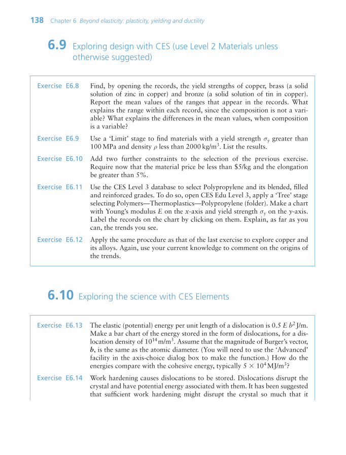
6.10 Exploring the science with CES Elements
6.9 Exploring design with CES (use Level 2 Materials unlessotherwise suggested)
138 Chapter 6 Beyond elasticity: plasticity, yielding and ductility
Exercise E6.8 Find, by opening the records, the yield strengths of copper, brass (a solidsolution of zinc in copper) and bronze (a solid solution of tin in copper).Report the mean values of the ranges that appear in the records. Whatexplains the range within each record, since the composition is not a vari-able? What explains the differences in the mean values, when compositionis a variable?
Exercise E6.9 Use a ‘Limit’ stage to find materials with a yield strength σy greater than100 MPa and density ρ less than 2000 kg/m3. List the results.
Exercise E6.10 Add two further constraints to the selection of the previous exercise.Require now that the material price be less than $5/kg and the elongationbe greater than 5%.
Exercise E6.11 Use the CES Level 3 database to select Polypropylene and its blended, filledand reinforced grades. To do so, open CES Edu Level 3, apply a ‘Tree’ stageselecting Polymers—Thermoplastics—Polypropylene (folder). Make a chartwith Young’s modulus E on the x-axis and yield strength σy on the y-axis.Label the records on the chart by clicking on them. Explain, as far as youcan, the trends you see.
Exercise E6.12 Apply the same procedure as that of the last exercise to explore copper andits alloys. Again, use your current knowledge to comment on the origins ofthe trends.
Exercise E6.13 The elastic (potential) energy per unit length of a dislocation is 0.5 E b2J/m.Make a bar chart of the energy stored in the form of dislocations, for a dis-location density of 1014m/m3. Assume that the magnitude of Burger’s vector,b, is the same as the atomic diameter. (You will need to use the ‘Advanced’facility in the axis-choice dialog box to make the function.) How do theenergies compare with the cohesive energy, typically 5 104MJ/m3?
Exercise E6.14 Work hardening causes dislocations to be stored. Dislocations disrupt thecrystal and have potential energy associated with them. It has been suggestedthat sufficient work hardening might disrupt the crystal so much that it
Ch06-H8391.qxd 1/16/07 5:48 PM Page 138

6.10 Exploring the science with CES Elements 139
becomes amorphous. To do this, the energy associated with the dislocationswould have to be about equal to the heat of fusion, since this is the differ-ence in energy between the ordered crystal and the disordered liquid. Theenergy per unit length of a dislocation is 0.5 E b2J/m. Explore this in the fol-lowing way:
(a) Calculate and plot the energy associated with a very high dislocationdensity of 1017m/m3 for the elements, i.e. plot a bar chart of0.5 1017 E b2 on the y-axis using twice atomic radius as equal toBurger’s vector b. Remember that you must convert GPa into kPa andatomic radius from nm to m to get the energy in kJ/m3.
(b) Now add, on the x-axis, the heat of fusion energy. Convert it fromkJ/mol to kJ/m3 by multiplying Hc by 1000/molar volume, with molarvolume in m3/kmol (as it is in the database). What, approximately, isthe ratio of the dislocation energy to the energy of fusion? Would youexpect this very high dislocation density to be enough to make thematerial turn amorphous?
Ch06-H8391.qxd 1/16/07 5:48 PM Page 139

This page intentionally left blank

Chapter 7Bend and crush:
strength-limited design
Chapter contents
7.1 Introduction and synopsis 1427.2 Standard solutions to plastic problems 1427.3 Material indices for yield-limited
design 1497.4 Case studies 1547.5 Summary and conclusions 1587.6 Further reading 1597.7 Exercises 1597.8 Exploring design with CES 161
Elastic design, avoiding plasticity, ensures that thecabin of the car does not deform in a crash. Plasticityabsorbs the energy of impact, and allows metals tobe shaped and polymers to be molded. (Image of
crash testing courtesy AutoNews; image of hot rollingcourtesy of Tanis Inc., Delafield, WI.)
Ch07-H8391.qxd 1/16/07 5:53 PM Page 141

142 Chapter 7 Bend and crush: strength-limited design
7.1 Introduction and synopsis
Stiffness-limited design, described in Chapter 5, is design to avoid excessiveelastic deflection. Strength-limited design, our concern here, is design to avoidplastic collapse. That generally means design to avoid yield, arranging that thecomponent remains elastic throughout, when it is called elastic design. Elasticdesign is not always possible or necessary: local yielding may be permissibleprovided general yield is avoided.
That is half the picture. The other half is design to permit controlled plastic col-lapse. The safety of modern cars relies on the front of the car absorbing the kineticenergy in a collision by plastic deformation. And the manufacturing processesof metal rolling, forging, extrusion and pressing use plastic flow. Here, strainsare large, elastic deformation irrelevant, and the focus is on the forces andwork necessary to achieve a prescribed change of shape (see cover picture).
Plasticity problems are solved in more than one way. When yield is to beavoided, we analyze the elastic state of stress in a component and make sure thatthis nowhere exceeds the yield strength. Full plasticity, by contrast, requiresgeneral yield. Then the mechanism of plastic collapse must be identified and thecollapse load calculated by requiring that yield does occur where it needs to.
Chapter 5 introduced elastic solutions for common modes of loading: ten-sion, compression, bending, torsion or internal pressure. Not surprisingly thereare equivalent results for plastic design, and we start with these. As before, youdon’t need to know how to derive them, just where to find them and how to usethem. We use them to develop material indices for strength-limited design andapply them via case studies.
7.2 Standard solutions to plastic problems
Yielding of ties and columnsA tie is a rod loaded in tension, a column is a rod loaded in compression. Thestate of stress within them is uniform, as was shown in Figure 5.1(a). If thisstress, σ, is below the yield strength σy the component remains elastic; if itexceeds σy, it yields. Yield in compression is only an issue for short, squatcolumns. Slender columns and panels in compression are more likely to buckleelastically first (Chapter 5).
Yielding of beams and panelsThe stress state in bending was introduced in Chapter 5. A bending moment Mgenerates a linear variation of longitudinal stress σ across the section (Figure7.1(a)) defined by
(7.1)σκ
yMI
E
Ch07-H8391.qxd 1/16/07 5:53 PM Page 142

7.2 Standard solutions to plastic problems 143
where y is the distance from the neutral axis, and the influence of the cross-section shape is captured by I, the second moment of area. For elastic deflec-tion, we were interested in the last term in the equation—that containing thecurvature κ. For yielding, it is the first term. The maximum longitudinal stressσmax occurs at the surface (Figure 7.1(a)), at the greatest distance ym from theneutral axis
(7.2)
The quantity Ze I/ym is called the elastic section modulus (not to be confusedwith the elastic modulus of the material, E). If σmax exceeds the yield strengthσy of the material of the beam, small zones of plasticity appear at the surfacewhere the stress is highest, as in Figure 7.1(b). The beam is no longer elasticand, in this sense, is damaged even if it has not failed completely. If the momentis increased further, the linear profile is truncated—the stress near the surface
σmaxm
e
M y
IMZ
1/κ
σ
y Tension
Compression
σ
y Tension
Compression
σy
σy
σy
σy
(a) Elastic
(b) Onset of plasticity
(c) Full plasticity
Plastic zone
Plastic zone
yy Tension
Compression
M MNeutral
axisStress
σσ
Figure 7.1 A beam loaded in bending. The stress state is shown on the right for purelyelastic loading (a), the onset of plasticity (b), and full plasticity (c).
Ch07-H8391.qxd 1/16/07 5:53 PM Page 143
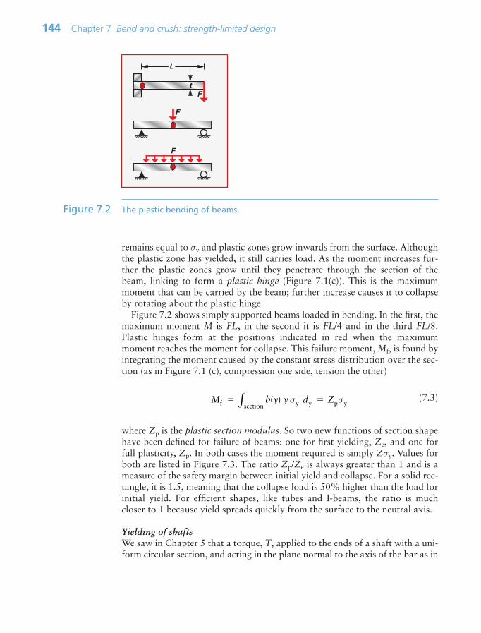
remains equal to σy and plastic zones grow inwards from the surface. Althoughthe plastic zone has yielded, it still carries load. As the moment increases fur-ther the plastic zones grow until they penetrate through the section of thebeam, linking to form a plastic hinge (Figure 7.1(c)). This is the maximummoment that can be carried by the beam; further increase causes it to collapseby rotating about the plastic hinge.
Figure 7.2 shows simply supported beams loaded in bending. In the first, themaximum moment M is FL, in the second it is FL/4 and in the third FL/8.Plastic hinges form at the positions indicated in red when the maximummoment reaches the moment for collapse. This failure moment, Mf, is found byintegrating the moment caused by the constant stress distribution over the sec-tion (as in Figure 7.1 (c), compression one side, tension the other)
(7.3)
where Zp is the plastic section modulus. So two new functions of section shapehave been defined for failure of beams: one for first yielding, Ze, and one forfull plasticity, Zp. In both cases the moment required is simply Zσy. Values forboth are listed in Figure 7.3. The ratio Zp/Ze is always greater than 1 and is ameasure of the safety margin between initial yield and collapse. For a solid rec-tangle, it is 1.5, meaning that the collapse load is 50% higher than the load forinitial yield. For efficient shapes, like tubes and I-beams, the ratio is muchcloser to 1 because yield spreads quickly from the surface to the neutral axis.
Yielding of shaftsWe saw in Chapter 5 that a torque, T, applied to the ends of a shaft with a uni-form circular section, and acting in the plane normal to the axis of the bar as in
M b y y d Zf y y p ysection( ) σ σ∫
144 Chapter 7 Bend and crush: strength-limited design
F
F
F
L
t
Figure 7.2 The plastic bending of beams.
Ch07-H8391.qxd 1/16/07 5:53 PM Page 144

Figure 7.4, produces a shear stress that increases linearly with distance r fromthe central axis:
(7.4)
where K is the polar second moment of area. The resulting elastic deformationwas described by the angle of twist per unit length θ/L. Failure occurs when the
τθ
T rK
G rK
7.2 Standard solutions to plastic problems 145
Section shapeArea A Elastic section
modulus Ze
Plastic sectionmodulus Zp m3
b h6hb 2
4hb 2
2rπ 3r4π 3r
3π
tr2
)rr( 2i
2o
π
−π
tr
)rr(r4
2
4i
4o
o
π
−π
tr
)rr(3
2
3i
3o
π
−π
m3m2
h
b
2r
2ro
t
2ri
Figure 7.3 The area A, section modulus Ze and fully plastic modulus Zp for three simplesections.
L
d i do
d
F
F,u
F
d
R
Shafts Helical springs
Yield
Fracture
T Tsfr
T Tsy
2
Figure 7.4 Elastic torsion of shafts. The stress in the shaft depends on the torque T and thepolar moment of area K. Helical springs are a special case of torsional loading.
Ch07-H8391.qxd 1/16/07 5:53 PM Page 145
maximum surface stress exceeds the yield strength σy of the material. The max-imum shear stress, τmax, is at the surface and has the value
(7.5)
where R is the radius of the shaft. From Chapter 6, the yield stress in shear, k,is half the tensile yield stress, so first yield occurs when τmax σy /2. When thetorque is increased further, plasticity spreads inwards. The maximum torquethat the shaft can carry occurs when τ k over the whole section. Any greatertorque than this causes the shaft to collapse in torsion by unrestrained rotation.For example, for a solid circular section, the collapse torque is
(7.6)
Helical springs are a special case of torsional loading (Figure 7.4): when thespring is loaded axially, the individual turns twist. It is useful to know the springstiffness, S. If the spring has n turns of wire of shear modulus G, each of diam-eter d, wound to give a spring of radius R, the stiffness is
where F is the axial force applied to the spring and u is its extension. The elas-tic extension is limited by the onset of plasticity. This occurs at the force
(7.7)
Spinning disks (flywheels)Spinning disks or rings store kinetic energy U (Figure 7.5). Centrifugal forcesgenerate a radial tensile stress in the disk that reaches a maximum value σmax.Analysis of a disk of density ρ, radius R and thickness t, rotating at an angularvelocity ω radians/second, gives the kinetic energy and the maximum stress(when Poisson’s ratio is taken as 1/3) as
(7.8)U t R R π
ρ ω σ ρ ω4
and 0.422 4max
2 2
Fd
Rcrit
3y
32
π σ
SFu
G dn R
4
364
T r k23
3π
τmax T RK
146 Chapter 7 Bend and crush: strength-limited design
Ch07-H8391.qxd 1/16/07 5:53 PM Page 146

The disk yields when σmax exceeds σy, and this defines the maximum allowableω and limits the inertial energy storage.
Contact stressesContact stress analysis is important in design of rolling and sliding contacts asin bearings, gears and railway track. Yielding at contacts is closely linked tofailure by wear and fatigue. When surfaces are placed in contact they touch ata few discrete points. If the surfaces are loaded, the contacts flatten elasticallyand the contact areas grow (Figure 7.6). The stress state beneath the contact iscomplex, first analyzed by the very same Hertz1 for whom the unit of frequencyis named. Consider a sphere of radius R made of material of Young’s modulus
7.2 Standard solutions to plastic problems 147
s
t
R
ω
Figure 7.5 Spinning disks, as in flywheels and gyroscopes, carry radial tensile stress causedby centrifugal force.
R
u
2a
F
ν = 13
Onset of plasticity
Figure 7.6 Contact stresses are another form of stress concentration. When elastic, thestresses and displacement of the surfaces towards each other can be calculated.
1 Heinrich Rudolph Hertz (1821–1894), German physicist, discoverer of radio waves andhow to generate them and inventor of the transmitter that started the radio age. In hisspare time he dabbled in mechanics.
Ch07-H8391.qxd 1/16/07 5:53 PM Page 147
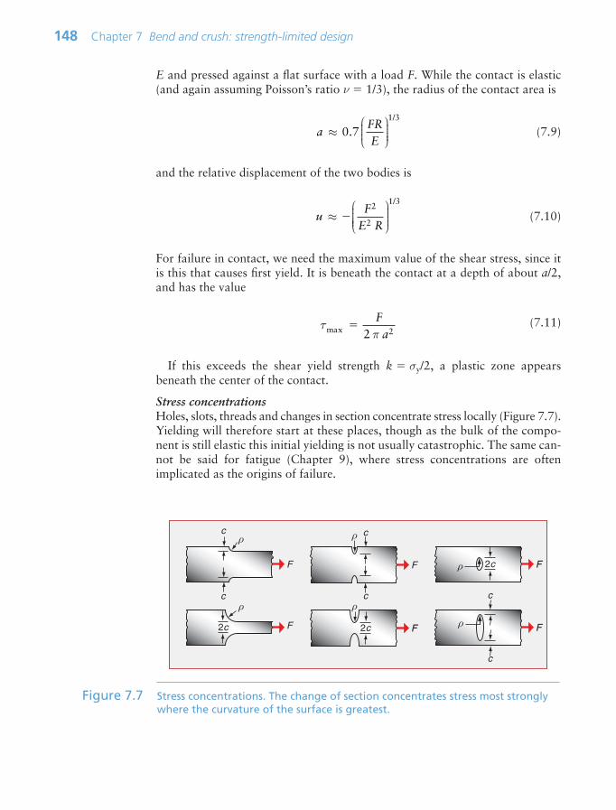
E and pressed against a flat surface with a load F. While the contact is elastic(and again assuming Poisson’s ratio ν 1/3), the radius of the contact area is
(7.9)
and the relative displacement of the two bodies is
(7.10)
For failure in contact, we need the maximum value of the shear stress, since itis this that causes first yield. It is beneath the contact at a depth of about a/2,and has the value
(7.11)
If this exceeds the shear yield strength k σy/2, a plastic zone appearsbeneath the center of the contact.
Stress concentrationsHoles, slots, threads and changes in section concentrate stress locally (Figure 7.7).Yielding will therefore start at these places, though as the bulk of the compo-nent is still elastic this initial yielding is not usually catastrophic. The same can-not be said for fatigue (Chapter 9), where stress concentrations are oftenimplicated as the origins of failure.
τπmax 22
F
a
uF
E R≈
⎛
⎝⎜⎜⎜⎜
⎞
⎠⎟⎟⎟⎟
2
2
1/3
aFRE
≈⎛
⎝⎜⎜⎜
⎞
⎠⎟⎟⎟⎟0.71/3
148 Chapter 7 Bend and crush: strength-limited design
F2c
ρ
F2cρF
c
c
ρ
Fρ
c
c
F
c
c
ρ
F2c
ρ
Figure 7.7 Stress concentrations. The change of section concentrates stress most stronglywhere the curvature of the surface is greatest.
Ch07-H8391.qxd 1/16/07 5:53 PM Page 148

We define the nominal stress in a component σnom as the load divided by thecross-section, ignoring features that cause the stress concentration. The maxi-mum local stress σmax is then found approximately by multiplying the nominalstress σnom by a stress concentration factor Ksc, where
(7.12)
Here ρsc is the minimum radius of curvature of the stress-concentrating featureand c is a characteristic dimension associated with it: either the half-thicknessof the remaining ligament, the half-length of a contained notch, the length ofan edge notch or the height of a shoulder, whichever is least (Figure 7.7). Thefactor α is roughly 2 for tension, but is nearer 1/2 for torsion and bending.Though inexact, the equation is an adequate working approximation for manydesign problems. More accurate stress concentration factors are tabulated incompilations such as Roark (see ‘Further reading’ at the end of this chapter).
As a simple example, consider a circular hole in a plate loaded in tension. Theradius of curvature of the feature is the hole radius, ρsc R, and the character-istic dimension is also the radius, c R. From equation (7.12), the local stressnext to the hole is thus three times the nominal tensile stress—however smallthe hole. Local yielding therefore occurs when the nominal stress is only σy/3.
7.3 Material indices for yield-limited design
Minimizing weight: a light, strong tie-rodMany structures rely on tie members that must carry a prescribed tensile loadwithout yielding—the cover picture of Chapter 4 showed two—often with therequirement that they be as light as possible. Consider a design that calls for acylindrical tie-rod of given length L that must carry a tensile force F as in Figure5.7(a), with the constraint that it must not yield, but remain elastic. The objec-tive is to minimize its mass. The length L is specified but the cross-section areaA is not (Table 7.1).
As before, we first seek an equation describing the quantity to be maximizedor minimized. Here it is the mass m of the tie
m ALρ (7.13)
where A is the area of the cross-section and ρ is the density of the material ofwhich it is made. We can reduce the mass by reducing the cross-section, butthere is a constraint: the section area A must be sufficient to carry the tensileload F without yielding, requiring that
Kc
scmax
nom sc
1/2
1 σσ
αρ
⎛
⎝⎜⎜⎜⎜
⎞
⎠⎟⎟⎟⎟⎟
7.3 Material indices for yield-limited design 149
Ch07-H8391.qxd 1/16/07 5:53 PM Page 149
(7.14)
where σy is the yield strength. Eliminating A between these two equations gives
(7.15)
The lightest tie that will carry F safely is that made of the material with thesmallest value of ρ/σy. We could define this as the material index of the prob-lem, seeking a minimum, but as in Chapter 5 we will invert it, seeking materi-als with the largest values of
(7.16)
This index, the specific strength, is plotted as a line of slope 1 in the chart ofFigure 7.8. A particular value of σy/ρ is identified, passing through the high-strength end of several major alloy systems—nickel alloys, high-strength steels,and aluminum and magnesium alloys. Titanium alloys are significantly betterthan the other metals; CFRP is better still. Ceramics and glasses have high val-ues of Mt but are impractical as structural ties because of their brittleness.
Tension, then, is straightforward. The real problem in elastic design is sel-dom tension; it is bending. We therefore revisit the bending of panels andbeams, applying a constraint on strength rather than stiffness.
Minimizing weight: light, strong panelsFigure 5.7(b) showed a panel supported at its edges, carrying a specified centralload. The width b and span L are fixed, but we are free to choose the thicknessh. The objective is to minimize the mass. Reducing the thickness reduces themass, but it must be sufficient for the maximum stress to be below the elasticlimit (Table 7.2).
Mty
σ
ρ
m F Lρ
σy
⎛
⎝
⎜⎜⎜⎜⎜
⎞
⎠
⎟⎟⎟⎟⎟⎟
FA
σy
150 Chapter 7 Bend and crush: strength-limited design
Function • Tie-rod
Constraints • Length L specified• Tie must support tensile load F without yielding
Objective • Minimize the mass m of the tie
Free variables • Choice of cross-section area, A• Choice of material
Table 7.1 Design requirements for the light tie
Ch07-H8391.qxd 1/16/07 5:53 PM Page 150

The procedure is much as before—set up an equation for the mass; find anexpression for the maximum stress (noting that for a rectangular section,I bh3/12); use this constraint to eliminate the free variable h and read off thematerial index. The analysis itself is left for the Exercises; the result is
(7.17)
This index is also shown by a shaded guideline in Figure 7.8. Now all the lightalloys (Mg, Al and Ti) outperform steel, as do GFRP and wood. CFRP stillleads the way.
Mpy1/2
σ
ρ
7.3 Material indices for yield-limited design 151
Density, ρ (Mg/m3)
0.01
Str
engt
h, σ
y or
σel
(MP
a)
0.01
100.1 1
0.1
1
10
100
1000
10000
PE
Woods,
T
Foams
Polymers and elastomers
MetalsCeramics
Composites
Natural materials
Lead alloys
Tungsten alloys
SteelsTi alloys
Mg alloys
CFRP
GFRP
Al alloys
Rigid polymer foams
Flexible polymer foams
Ni alloys
Copper alloys
Zinc alloys
PAPEEK
PMMAPC
PET
Cork
Woods, ll
Butyl rubber
Silicone elastomers
Concrete
Tungstencarbide
Al2O3SiC
Si3N4Strength–Density
MFA, 07
σf1/2
ρ
σf2/3
ρ
σfρ
Guide lines for minimum mass
design
Metals and polymers: yield strengthCeramics and glasses: MORElastomers: tensile tear strengthComposites: tensile failure
MssNi a
ETSearchregion
oams
s
Tun
A
T
Mb= σy /ρ2/3
Mt = σy /ρ
Mp= σy /ρ1/2
Figure 7.8 The strength–density chart with the indices σy/ρ, σ2/3y /ρ and σy
1/2/ρ plotted on it.
Function • Panel in bending
Constraints • Width b and span L specified• Panel must support bending load F without yielding
Objective • Minimize the mass m of the panel
Free variables • Choice of thickness h• Choice of material
Table 7.2 Design requirements for the light panel
Ch07-H8391.qxd 1/16/07 5:53 PM Page 151

Light, strong beams: the effect of shapeIn beam design we are free to choose the shape as well as the dimensions of thecross-section. First we consider beams of prescribed shape, with freedom tochange their size in a self-similar way. Then we explore how much better we canmake the design by using efficient shapes.
Start with the beam of square section A b b, which may vary in size,loaded in bending over a span of fixed length L with a central load F (Figure5.7(c) and Table 7.3).
The analysis is similar to the panel (see Exercises), with the modified secondmoment of area, I b4/12 A2/12. The resulting material index is
(7.18)
The chart in Figure 7.8 shows that the slope of this index lies between the othertwo, so the competition between metals, wood and composites changes again,with CFRP still on top.
But, you will say, no one uses solid, square-section, beams for minimum massdesign—and you are right. If you want to support bending loads it is better tochoose a shape that uses less material to provide the same strength. Woodenfloor-joists in houses are typically twice as deep as they are wide; standard steeland aluminum beams have an I-section or a box section; space frames, commonly,are made from tubes. Does this change the index? Well, yes and no. Start withthe no.
Equation (7.18) was derived by analyzing a square beam, but the result holdsfor any self-similar shape, meaning one in which all dimensions remain in pro-portion as the size is varied. Shaping a given cross-sectional area from a solidsquare beam into a tube or an I-beam increases the second moment of area,without changing the cross-sectional area or the mass. In Chapter 5, it wasshown that this provides greater stiffness with no mass penalty. It also makesthe beam stronger. Equation (7.2) shows that a bending moment gives a maxi-mum stress determined by the elastic section modulus, Ze I/ym. Consequentlythe gain in strength by increasing I is not quite as great as the gain in stiffness—shaping the section to an I-beam increases I, but usually makes the beam deeper
Mby2/3
σ
ρ
152 Chapter 7 Bend and crush: strength-limited design
Function • Beam in bending
Constraints • Span L specified, section shape square• Beam must support bending load F without yielding
Objective • Minimize the mass m of the beam
Free variables • Area A (or square section dimension b)• Choice of material
Table 7.3 Design requirements for the light strong beam
Ch07-H8391.qxd 1/16/07 5:53 PM Page 152
too, increasing ym. As before, we can define a ‘shape factor’ φ yB for strength—
the ratio of Ze for the shaped section to Ze for the same area of material in asolid square section:
Recall from Chapter 5 that materials are not all equally easy to shape; if theywere, all could be given the same efficient shape and the index in equation(7.18) would be sufficient. Table 7.4 gives typical upper values of the shape fac-tor for strength, for a range of competing materials.
The right-hand column of Table 7.4 shows the corresponding mass savingwe might achieve by shaping and using less material to carry the same load inbending. Metals and composites can all be improved significantly (thoughagain metals do a little better), but wood has more limited potential. So, whencomparing materials for light, strong beams using the index in equation (7.18),the performance of wood should not be overestimated; other materials allowmore efficient shapes.
Minimizing material cost or volumeWhen the objective is to minimize cost rather than weight, the indices changeexactly as before. The objective function for the material cost C of the tie, panelor beam becomes
C mCm ALCmρ (7.19)
where Cm is the cost per kg of the material. This leads to indices which are justthose of equations (7.16)–(7.18) with ρ replaced by Cm ρ.
If instead the objective is to minimize volume, density is no longer relevant.The indices for ties, panels and beams are then the same as those for minimummass with ρ deleted.
φBy e
shaped
esolid
Z
Z
7.3 Material indices for yield-limited design 153
Material Maximum failure shape Mass ratio by shapingfactor (failure moment (relative to solid squarerelative to solid square beam)beam) φy
B
Steels 13 0.18Al alloys 10 0.22Composites 9 0.23(GFRP, CFRP)Wood 3 0.48
Table 7.4 The effect of shaping on strength and mass of beams in different structuralmaterials
Ch07-H8391.qxd 1/16/07 5:53 PM Page 153

7.4 Case studies
Plasticity problems are of two types. In the first yield is avoided everywhere sothat the entire component remains elastic, meeting the condition σ σy every-where. Limited local plastic flow at stress concentrations may be allowed pro-vided that, once it has happened, the condition σ σy is met everywhere (beddingdown). In the second, full plasticity is the aim. Manufacturing processes suchas metal forging and extrusion are well-managed plasticity; crash barriers andpackaging, too, rely on full plasticity to absorb energy.
First a cautionary note. Carrying loads safely is not just a question of strength,but also of toughness—the resistance of the material to fracture. Strength andtoughness are not the same thing—we explain why in the next chapter. Fornow, it is enough to know that some materials may appear to be good optionsfor strength-limited design, but that they are impractical because they are toobrittle in tension or in shock loading.
Corkscrew levers again: strengthThe lever of the corkscrew of Figure 5.13 and described in Section 5.5 is loadedin bending. It needs some stiffness, but if it flexes slightly, no great harm is done.If, however, it yields, bending permanently before it extracts the cork, the userwill not be happy. So it must also meet a strength constraint.
The cross-section is rectangular. As in Chapter 5 we make the assumption ofself-similarity, meaning that we are free to change the scale of the section butnot its shape. Then the criterion for selection is that of the index of equation(7.18), Mb σ2/3
y/ρ. The index is plotted in Figure 7.8, isolating materials forlight, strong beams. The selection is almost the same as that for stiffness: CFRP,magnesium and aluminum alloys are the best choice.
But what about the stress-concentrating effect at the holes? A stress concen-tration factor Ksc means that yield starts when the nominal stress exceeds σy/Ksc.Changing the scale of the part does not change Ksc because it depends only onthe shape of the defect—the ratio ρ/c (its value for a circular hole is 3, regard-less of scale), with the result that the index remains unchanged and the selectionremains valid.
Elastic hinges and couplingsNature makes much use of elastic hinges: skin, muscle, cartilage all allow large,recoverable deflections. Man, too, designs with flexural and torsional hinges:ligaments that connect or transmit load between components while allowinglimited relative movement between them by deflecting elastically (Figures 5.18and 5.19). Which materials make good hinges?
Consider the hinge for the lid of a box. The box, lid and hinge are to be moldedin one operation—there are no separate screws or pins. The hinge is a thin lig-ament of material that flexes elastically as the box is closed, as in Figure 5.18, butit carries no significant axial loads. Then the best material is the one that (for givenligament dimensions) bends to the smallest radius without yielding or failing.
154 Chapter 7 Bend and crush: strength-limited design
Ch07-H8391.qxd 1/16/07 5:53 PM Page 154
When a ligament of thickness t is bent elastically to a radius R, the surfacestrain is
(7.20)
and—since the hinge is elastic—the maximum stress is
This must not exceed the yield or failure strength σy. Thus, the minimum radiusto which the ligament can be bent without damage is
(7.21)
The best material is the one that can be bent to the smallest radius—that is, theone with the greatest value of the index
(7.22)
Here we need the σy E chart (Figure 7.9). Candidates are identified by usingthe guideline of slope 1; a line is shown at the position M σy/E 3 102.The best choices for the hinge are all polymeric materials. The short-list includespolyethylene, polypropylene, nylon and, best of all, elastomers, though thesemay be too flexible for the body of the box itself. Cheap products with this sortof elastic hinge are generally molded from polyethylene, polypropylene or nylon.Spring steel and other metallic spring materials (like phosphor bronze) are pos-sibilities: they combine usable σy/E with high E, giving flexibility with goodpositional stability (as in the suspensions of relays).
ME
σy
Rt E
2 yσ
⎡
⎣
⎢⎢⎢
⎤
⎦
⎥⎥⎥
σ EtR2
ε tR2
7.4 Case studies 155
Function • Elastic hinge
Constraint • No failure, meaning σ σy throughout the hinge
Objectives • Maximize elastic flexure
Free variables • Choice of material
Table 7.5 Design requirements for elastic hinges
Ch07-H8391.qxd 1/16/07 5:53 PM Page 155

Materials for springsSprings come in many shapes (Figure 7.10) and have many purposes: axialsprings (a rubber band, for example), leaf springs, helical springs, spiralsprings, torsion bars. All depend on storing elastic energy when loaded, releas-ing it when unloaded again. The stored energy per unit volume in a materialcarrying a tensile stress σ was derived in Chapter 4—it is given by σ2/2E. If thespring yields it deforms permanently and ceases to fulfill its function, so themaximum value of σ must not exceed σy, when the stored energy is σ2
y/2E perunit volume. The best material for a spring of minimum volume (Table 7.6) istherefore that with the greatest value of
(7.23)
While it is less obvious, the index is the same for leaf springs, torsional springand coil springs—the best choice for one is the best choice for all.
ME
σy
2
156 Chapter 7 Bend and crush: strength-limited design
Strength, σy or σel (MPa)
You
ng’s
mod
ulus
, E (
GP
a)
0.1 1 10 100 10000.01
0.1
1
10
100
1000
= 104
Yield strainσy
E
103
102101
Non-technical ceramics
MFA, 07
Foams
Polymers
MetalsTechnicalceramics
Composites
Lead alloys
W alloys
Ti alloys
Mg alloys
CFRP
GFRP
Al alloys
Rigid polymer foams
Ni alloys
Cu alloys
Zinc alloys
PMMA
Cork
Wood
Polyurethane
Silicone elastomers
Concrete
Al2O3
SiC
AlN
Modulus–StrengthB4C
EVA
Leather
Cast irons
WC
Soda glass
Silica glass
Silicon
Stone Brick
Epoxies
Ionomers
Steels
Polyurethane
PA
PC
PE
PTFE
PSPP
Phenolic
Metals and polymers: yield strengthCeramics and glasses: MORElastomers: tensile tear strengthComposites: tensile failure
σy2
E
σyE σy
3/2
E
Design guidelines
Elastomers
C
Mg a
GFRP
Al alloo
Zinc alZ
oys
CFRPCast ir
PAnolic
Searchregion
σy /E
iconeastoma
Leat
Io
ood
W alW
Phenoh
σy / E2
Figure 7.9 Materials for elastic hinges and springs. Polymers are the best choice for theformer. High-strength steel, CFRP, and certain polymers and elastomers are thebest choice for the latter.
Ch07-H8391.qxd 1/16/07 5:53 PM Page 156

The choice of materials for springs of minimum volume is shown in Figure7.9. A family of lines of slope 2 link materials with equal values of σ2
y/E; thosewith the highest values of M lie towards the bottom right. The heavy line is oneof the family; it is positioned so that a subset of materials is left exposed. Thebest choices are a high-strength steel lying near the top end of the line. Othermaterials are suggested too: CFRP (now used for truck springs), titanium alloys(good but expensive) and nylon (children’s toys often have nylon springs), and,of course, elastomers. Note how the procedure has identified a candidate fromalmost every class of materials: metals, polymers, elastomers and composites.
Full plasticity: metal rollingPlate, sheet, I-sections and sections like that of railroad track are shaped byrolling. Figure 7.11 shows the rolling of plate with an initial thickness t0. Theplate emerges from the rolls with a lesser thickness t1, a reduction of∆t t0 t1. A lower bound for the torque T and power P required to do thisis found from the plastic work, σyεpl per unit volume that it takes to produce aplastic strain εpl of ∆t/t0. If the rolls rotate through ∆θ a length R∆θ (and thus
7.4 Case studies 157
F
F,u
F
F
T
Figure 7.10 Springs: leaf, helical, spiral and torsion bar. Springs store energy. The bestmaterial for a spring, regardless of its shape or the way it is loaded, is that of amaterial with a large value of σ2
el/E.
Function • Elastic spring
Constraint • No failure, meaning stress below yieldthroughout the spring
Objectives • Maximum stored elastic energy per unit volume
Free variables • Choice of material
Table 7.6 Design requirements for springs
Ch07-H8391.qxd 1/16/07 5:53 PM Page 157

of volume V R∆θt0 per unit width) is fed into the ‘bite’, where it is com-pressed to the emerging thickness t1. Equating the work done by the pair ofrolls, 2T∆θ, to the plastic work V σyεpl gives the torque per roll:
(7.24)
The power P is just the torque times the angular velocity ω radians per second,giving
P 2Tω Rω σy ∆t (7.25)
The torque and power increase with σy so hot rolling takes less power than coldrolling because σy is smaller and work hardening (the increase of yield strengthwith strain) is negligible.
The values of T and P calculated here are lower bounds. Most metal-workingoperations involve redundant work (plastic work that is not strictly necessarybut happens anyway), friction as the compressed metal expands laterally andspeeds up in the gap, sliding against the roll surfaces, and work hardening, allof which increase the forces and power that is needed.
7.5 Summary and conclusions
Elastic design is design to avoid yield. That means calculating the maximum stress,σ, in a loaded component and ensuring that it is less than σy, the yield strength.Standard solutions give this maximum stress for panels, beams, torsion bars,spinning disks and many other components in terms of their geometry and theloads applied to them. From these, indices are derived to guide material choice.
T R t12 yσ ∆
158 Chapter 7 Bend and crush: strength-limited design
to
∆θ
R
T, ω
T, ω
t1
Figure 7.11 Rolling.
Ch07-H8391.qxd 1/16/07 5:53 PM Page 158

The indices depend on objectives such as minimizing mass or cost, much asthey did for stiffness limited design in Chapter 5.
Sometimes, however, controlled plasticity is the aim. Then the requirement isthat the stress must exceed the yield strength over the entire section of the com-ponent. Metal-forming operations such as forging, rolling and deep drawingrely on full plasticity. The forces and power they require scales with the yieldstrength of the material being shaped. Thus, soft metals such as lead, or purealuminum or low-carbon steel are easy to shape by plastic deformation, but someof the hardest, like tool steels and the nickel based super-alloys used in gas tur-bines, have such high yield strengths that they have to be shaped in other ways.
7.6 Further reading
Ashby, M.F. (2005) Materials Selection in Mechanical Design, 3rd edition, Butterworth-Heinemann, Oxford, UK, Chapter 4. ISBN 0-7506-6168-2. (Appendix A of this textis an expanded catalog of simple solutions to standard problems.)
Gere, J.M. (2006) Mechanics of Materials, 6th edition, Thompson Publishing, Toronto,Canada. ISBN 0-534-41793-0. (An intermediate level text on statics of structures byone of the fathers of the field; his books with Timoshenko introduced an entire gen-eration to the subject.)
Hosford, W.F. (2005) Mechanical Behavior of Materials, Cambridge University Press,Cambridge, UK. ISBN 0-521-84670-6. (A text that nicely links stress–strain behaviorto the micromechanics of materials.)
Jenkins, C.H.M. and Khanna, S.K. (2006) Mechanics of Materials, Elsevier Academic,Boston, MA, USA. ISBN 0-12-383852-5. (A simple introduction to mechanics,emphasizing design.)
Riley, W.F., Sturges, L.D. and Morris, D.H. (2003) Statics and Mechanics of Materials,2nd edition, McGraw-Hill, Hoboken, NJ, USA. ISBN 0-471-43446-9. (An intermedi-ate level text on the stress, strain and the relationships between them for many modesof loading. No discussion of micromechanics—response of materials to stress at themicroscopic level.)
Vable, M. (2002) Mechanics of Materials, Oxford University Press, Oxford, UK. ISBN0-19-513337-4. (An introduction to stress–strain relations, but without discussion ofthe micromechanics of materials.)
Young W.C. (1989) Roark’s Formulas for Stress and Strain, 6th edition, McGraw-Hill,New York, USA. ISBN 0-07-100373-8. (This is the ‘Yellow Pages’ of formulae forelastic problems—if the solution is not here, it doesn’t exist.)
7.7 Exercises
7.7 Exercises 159
Exercise E7.1 What is meant by the elastic section modulus, Ze? A beam carries a bendingmoment M. In terms of Ze, what is the maximum value M can take withoutinitiating plasticity in the beam?
Exercise E7.2 Derive the index for selecting materials for a light, strong panel, equation(7.17), following the steps outlined above the equation in the text.
Ch07-H8391.qxd 1/16/07 5:53 PM Page 159

160 Chapter 7 Bend and crush: strength-limited design
Exercise E7.3 Derive the index for selecting materials for a light, strong beam with a squarecross-section, equation (7.18).
Exercise E7.4 Derive an index for selecting materials for a panel that meets a constraint onbending strength and is as thin as possible.
Exercise E7.5 Derive an index for selecting materials for a panel that meets a constraint onbending strength and is as cheap as possible.
Exercise E7.6 A centrifuge has a rotor that can be idealized as a uniform disk. It has adiameter of 200 mm and is made of a material of strength 450 MPa and den-sity 7900 kg/m3. How fast can it be spun (in radians per second) before thestresses it carries exceed its yield strength?
Exercise E7.7 A material is sought for a high-speed centrifuge. The objective is to achieveas high an angular velocity ω of the centrifuge disk as possible. The con-straint is that the stress created by the centrifugal force must not exceed theyield strength of the material of which it is made. Derive an index to guide thechoice of material to allow the maximum ω.
Exercise E7.8 The engine of a car is mounted on four shear bolts designed to fail in shearin a front-end collision, detaching the engine from the car, if the decelerationexceeds 10 g. Assume that all four bolts carry the same load. The mass of theengine is 80 kg. Because of space limitations, the maximum diameter of eachshear bolt cannot exceed 5 mm. (a) Calculate the constraint on the yieldstrength σy of the material of the shear bolt, assuming that the shear strengthis σy/2 and that the mounting is done in such a way that the shear can takeplace without friction. (b) If, to save weight, the shear bolts have to be aslight as possible, what metal (of those identified in the chart of Figure 7.8)would you choose to make them?
Exercise E7.9 A plate with a rectangular section 500 mm by 15 mm carries a tensile load of50 kN. It is made of a ductile metal with a yield strength of 50 MPa. Theplate contains an elliptical hole of length 100 mm and a minimum radius of1 mm, oriented as shown in the diagram. What is:(a) The nominal stress?(b) The maximum stress in the plate?
Will the plate start to yield? Will it collapse completely?
Exercise E7.10 Valve springs for high-performance automobileengines must be light to minimize inertial loads sincepart of their mass moves with the valves; at highengine speeds the valves, if heavy, bounce out of con-tact with the valve itself (‘valve bounce’), impeding the flow of gas into and outof the combustion chamber. Derive the index for light springs to guide choice forthese, remembering that engine temperatures can reach 200°C.
100mm
500 mm
Radius 1 mm
50 kN
15 mm
Ch07-H8391.qxd 1/16/07 5:53 PM Page 160
7.8 Exploring design with CES (use Level 2 unless otherwiseindicated)
7.8 Exploring design with CES 161
Exercise E7.11 Use the ‘Search’ facility in CES to search for materials that are used forsprings. Report what you find.
Exercise E7.12 Use the ‘Search’ facility in CES to search for materials that are used for lightsprings. Report what you find.
Exercise E7.13 Make a property chart with σy on one axis and E on the other. Use it to selectmaterials for springs, using the index σ2
y/E derived in the text. Which threemetals emerge as the best metallic choices?
Exercise E7.14 A material is required for a spring that must be as light as possible. To be stiffenough it must also have a Young’s modulus E 20 GPa. Make a bar chartwith the index σ2
y/Eρ for selecting light springs derived in Exercise E7.10 (youwill need to use the ‘Advanced’ facility in the axis-choice dialog box to do this).Add a ‘Limit’ stage to apply the constraint E 20 GPa. Hence find the twomaterials that are the best choices for this application.
Exercise E7.15 Exercise E7.10 describes the requirements for valve springs for high-per-formance engines. Apply the index derived there, σ2
y/ρE, by making anappropriate chart and plotting an appropriate selection line on it. Enginesare hot: add a ‘Limit’ stage on maximum service temperature of 250°C.Hence select metals for this application.
Exercise E7.16 Abrasives have high hardness, H. Make a bar chart of hardness and identifythe four materials with the highest values. They are prime choices for abra-sive wheels and pastes.
Exercise E7.17 The text showed that the power required to roll a metal is proportional to itsyield strength. Make a bar chart of yield strength, σy for metals. Open therecord for low-carbon steel, find the range of its yield strength and take theaverage. Normalize all the yield strengths in the database by dividing themby this value, using the ‘Advanced’ option in the dialog box for selecting theaxes, so that low-carbon steel now lies at the value 1 on the bar chart. Usethe chart to read off how much less power is required to roll: (a) commer-cially pure zinc and (b) commercially pure lead at room temperature.
Exercise E7.18 Crash barriers, auto fenders and other protective structures rely on absorb-ing kinetic energy by plastic deformation. The energy Wpl absorbed indeforming a material to fracture (the area under the stress–strain curve) canbe estimated approximately in CES as
Wpl y ts f12
( ) σ σ ε
Ch07-H8391.qxd 1/16/07 5:53 PM Page 161

162 Chapter 7 Bend and crush: strength-limited design
Make a chart with density on the x-axis and Wpl on the y-axis by using the‘Advanced’ facility in the axis-selection dialog box. Use a box selection tofind the three materials that absorb the most energy. Rank them by price,using a ‘Graph’ stage to plot price.
Exercise E7.19 If the crash barrier of the last exercise is part of a vehicle, fuel is saved if it islight. We then want the materials with the largest value of Wpl/ρ, where ρ isthe density. These are found by using a selection line of slope 1 on the chartmade in the last exercise and selecting the materials above the line. In thisapplication the materials must also have adequate stiffness so that they do notbend elastically too much, requiring a Young’s modulus of at least 2.5 GPa.Apply this requirement using a ‘Limit’ stage, return to the chart and move theselection line until only three materials remain. Comment on the choice.
Exercise E7.20 Now explore what Level 3 of the database can do. Leave all the selectionlines and criteria in example E7.19. Go to File Change Database CESEdu Level 3 Open. A dialog box asks if you wish to apply this to your cur-rent project. Click on Yes. Then list the materials that now appear in theresults window. Comment on the choice.
Ch07-H8391.qxd 1/16/07 5:53 PM Page 162

Chapter 8Fracture and fracture
toughness
Chapter contents
8.1 Introduction and synopsis 1648.2 Strength and toughness 1648.3 The mechanics of fracture 1668.4 Material property charts for toughness 1728.5 Drilling down: the origins of toughness 1748.6 Manipulating properties: the 178
strength–toughness trade-off8.7 Summary and conclusions 1818.8 Further reading 1818.9 Exercises 1828.10 Exploring design with CES 1838.11 Exploring the science with CES
Elements 183
Ch08-H8391.qxd 1/17/07 10:45 AM Page 163
164 Chapter 8 Fracture and fracture toughness
8.1 Introduction and synopsis
It is easy to set a value on the engineering science that enables success, that makesthings happen, much harder to value engineering science that prevents failure,that stops things happening. One of the great triumphs of recent engineeringscience has been the development from the 1960s onwards of a rigorousmechanics of material fracture. We have no numbers for the money and lives ithas saved by preventing failures; all we know is that, by any measure, it is enor-mous. This chapter is about the ways in which materials fail when loaded pro-gressively, and design methods to ensure that fracture won’t happen unless youwant it to.
Sometimes, of course, you do. Aircraft engines are attached to the wing byshear-bolts, designed to fail and shed the engine if it suddenly seizes. At a morefamiliar level, peel-top cans, seals on food containers and many other safetydevices rely on controlled tearing or fracture. And processes like machining andcutting use a combination of plasticity and fracture.
We start by distinguishing strength from toughness. Toughness—resistanceto fracture—requires a new material property, the fracture toughness devel-oped in Section 8.3, to describe it. This new property is explored in Section 8.4using charts like those we have already seen for modulus and strength. Theunderlying science mechanisms (Section 8.5) give insight into ways in whichtoughness can be manipulated (Section 8.6). The chapter ends in the usual waywith a summary, Further reading and Exercises.
8.2 Strength and toughness
Strength and toughness? Why both? What’s the difference?Strength, when speaking of a material, is its resistance to plastic flow. Think ofa sample loaded in tension. Increase the stress until dislocations sweep rightacross the section, meaning the sample just yields, and you measure the initialyield strength. Strength generally increases with plastic strain because of workhardening, reaching a maximum at the tensile strength. The area under the wholestress–strain curve up to fracture is the work of fracture. We’ve been herealready—it was the subject of Chapter 5.
Toughness is the resistance of a material to the propagation of a crack. Supposethat the sample of material contained a small, sharp crack, as in Figure 8.1(a).The crack reduces the cross-section A and, since stress σ is F/A, it increases thestress. But suppose the crack is small, hardly reducing the section, and the sam-ple is loaded as before. A tough material will yield, work harden and absorbenergy as before—the crack makes no significant difference. But if the materialis not tough (defined in a moment) then the unexpected happens; the crack sud-denly propagates and the sample fractures at a stress that can be far below theyield strength. Design based on yield is common practice. The possibility of fracture
Ch08-H8391.qxd 1/17/07 10:45 AM Page 164

8.2 Strength and toughness 165
at stresses below the yield strength is really bad news. And it has happened, onspectacular scales, causing boilers to burst, bridges to collapse, ships to breakin half, pipelines to split and aircraft to crash. We get to that in Chapter 10.
So what is the material property that measures the resistance to the propaga-tion of a crack? And just how concerned should you be if you read in the paperthat cracks have been detected in the track of the railway on which you com-mute or in the pressure vessels of the nuclear reactor of the power station a fewmiles away? If the materials are tough enough you can sleep in peace. But whatis ‘tough enough’?
This difference in material behavior, once pointed out, is only too familiar.Buy a CD, a pack of transparent folders or even a toothbrush: all come in per-fect transparent packaging. Try to get them out by pulling and you have a prob-lem: the packaging is strong. But nick it with a knife or a key or your teeth andsuddenly it tears easily. That’s why the makers of shampoo sachets do the nickfor you. What they forget is that the polymer of the sachet becomes tougherwhen wet, and that soapy fingers can’t transmit much force. But they had theright idea.
Tests for toughnessIf you were asked to devise a test to characterize toughness, you might dreamup something like those of Figure 8.2: notch the material, then yank it orwhack it till it breaks, measuring the energy to do so. Tests like these (there aremany variants) are in fact used for ranking and as an acceptance procedurewhen taking delivery of a new batch of material. The problem is that they donot measure a true material property, meaning one that is independent of thesize and shape of the test sample, so the energy measurements do not help withdesign. To get at the real, underlying, material properties we need the ideas ofstress intensity and fracture toughness.
Crack
Plasticity
(b) Tough behavior
Fracture
FF
(c) Brittle behavior(a) Cracked sample
Figure 8.1 Tough and brittle behavior. The crack in the tough material, shown in (b), doesnot propagate when the sample is loaded; that in the brittle material propagateswithout general plasticity, and thus at a stress less than the yield strength.
Ch08-H8391.qxd 1/17/07 10:45 AM Page 165

8.3 The mechanics of fracture
Stress intensity Kl and fracture toughness KlcCracks concentrate stress. A remote stress σ applies a force that is transmittedthrough a cracked material in the way suggested by Figure 8.3. The local stress,σlocal, which is proportional to the number of lines of force crossing unit lengthof cross-section, is non-uniform, rising steeply as the crack tip is approached.The stress concentration factor, defined for notches and holes in Chapter 7,does not help here—it is relevant only for features with a finite radius of curva-ture. Cracks are sharp—the radius at the tip is essentially zero. Analysis of thestress field ahead of a sharp crack of length c shows that the local stress at a dis-tance r from its tip caused by a remote uniform tensile stress σ is
(8.1)
where Y is a constant with a value near unity that depends weakly on the geom-etry of the cracked body. Far from the crack, where r c, the local stress fallsto the value σ, but near the tip, where r c, it rises steeply, as
(8.2)
So for any given value of r the local stress scales as which therefore is ameasure of the intensity of the local stress (the inclusion of the π is a convention
σ πc
σσ π
πlocal
2 Y
c
r
σ σππlocal 1
2 Y
cr
⎛
⎝
⎜⎜⎜⎜⎜
⎞
⎠
⎟⎟⎟⎟⎟
166 Chapter 8 Fracture and fracture toughness
Load
Extension
Initiation energy
Propagation energy
(a)
Impact energyU = m g ∆h ∆h
Mass m
Sample
(b)
Figure 8.2 (a) The tear test. (b) The impact test. Both are used as acceptance tests and forquality control, but neither measures a true material property.
Ch08-H8391.qxd 1/17/07 10:45 AM Page 166
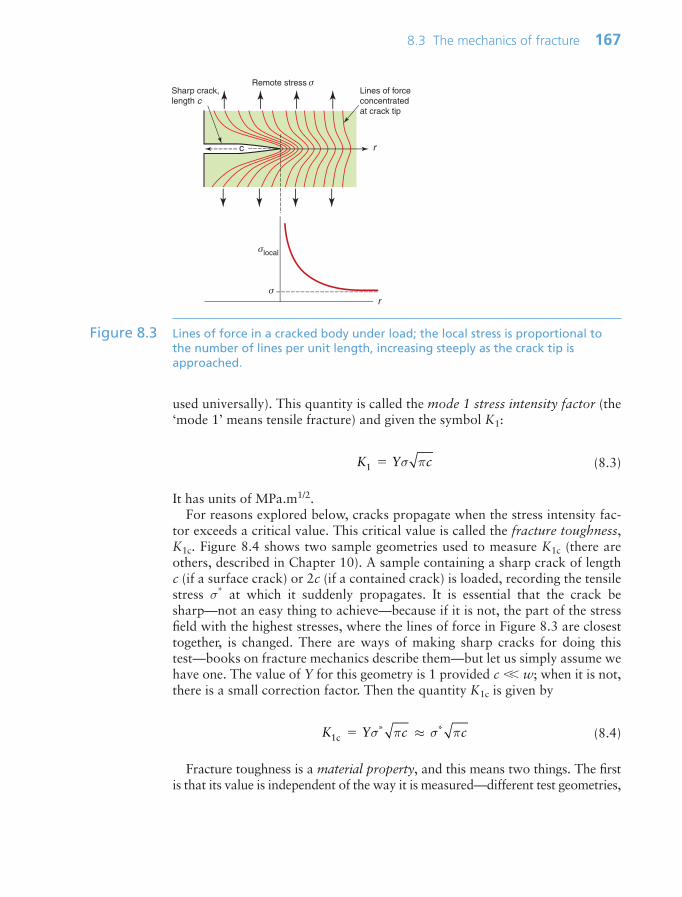
used universally). This quantity is called the mode 1 stress intensity factor (the‘mode 1’ means tensile fracture) and given the symbol K1:
(8.3)
It has units of MPa.m1/2.For reasons explored below, cracks propagate when the stress intensity fac-
tor exceeds a critical value. This critical value is called the fracture toughness,K1c. Figure 8.4 shows two sample geometries used to measure K1c (there areothers, described in Chapter 10). A sample containing a sharp crack of lengthc (if a surface crack) or 2c (if a contained crack) is loaded, recording the tensilestress σ* at which it suddenly propagates. It is essential that the crack besharp—not an easy thing to achieve—because if it is not, the part of the stressfield with the highest stresses, where the lines of force in Figure 8.3 are closesttogether, is changed. There are ways of making sharp cracks for doing thistest—books on fracture mechanics describe them—but let us simply assume wehave one. The value of Y for this geometry is 1 provided c w; when it is not,there is a small correction factor. Then the quantity K1c is given by
(8.4)
Fracture toughness is a material property, and this means two things. The firstis that its value is independent of the way it is measured—different test geometries,
K Y c c1c* * σ π σ π≈
K Y c1 σ π
8.3 The mechanics of fracture 167
Remote stress σLines of forceconcentrated at crack tip
c r
σlocal
σr
Sharp crack,length c
Figure 8.3 Lines of force in a cracked body under load; the local stress is proportional tothe number of lines per unit length, increasing steeply as the crack tip isapproached.
Ch08-H8391.qxd 1/17/07 10:45 AM Page 167
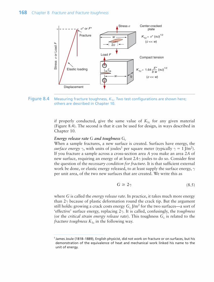
if properly conducted, give the same value of K1c for any given material (Figure 8.4). The second is that it can be used for design, in ways described inChapter 10.
Energy release rate G and toughness GcWhen a sample fractures, a new surface is created. Surfaces have energy, thesurface energy γ, with units of joules1 per square meter (typically γ 1 J/m2).If you fracture a sample across a cross-section area A you make an area 2A ofnew surface, requiring an energy of at least 2Aγ joules to do so. Consider firstthe question of the necessary condition for fracture. It is that sufficient externalwork be done, or elastic energy released, to at least supply the surface energy, γper unit area, of the two new surfaces that are created. We write this as
(8.5)
where G is called the energy release rate. In practice, it takes much more energythan 2γ because of plastic deformation round the crack tip. But the argumentstill holds: growing a crack costs energy Gc J/m2 for the two surfaces—a sort of‘effective’ surface energy, replacing 2γ. It is called, confusingly, the toughness(or the critical strain energy release rate). This toughness Gc is related to thefracture toughness K1c in the following way.
G 2γ
168 Chapter 8 Fracture and fracture toughness
K1c = σ* (πc)1/2
Str
ess
σ o
r Lo
ad F
Displacement
σ* or F*
Fracture
Elastic loading
2c
Stress σ
w
c
w b
(c << w)
Load F
(c << w)
K1c = 1.64 (πc)1/2 F*
b w
Center-cracked plate
Compact tension
Figure 8.4 Measuring fracture toughness, K1c. Two test configurations are shown here;others are described in Chapter 10.
1James Joule (1818–1889), English physicist, did not work on fracture or on surfaces, but hisdemonstration of the equivalence of heat and mechanical work linked his name to theunit of energy.
Ch08-H8391.qxd 1/17/07 10:45 AM Page 168

Think of a slab of material of unit thickness carrying a stress σ. The elasticenergy stored in it (Chapter 4) is
(8.6)
per unit volume. Now put in a crack of length c, as in Figure 8.5. The crackrelaxes the stress in a half-cylinder of radius about c—the reddish half-cylinderin the figure—releasing the energy it contained:
(8.7)
Suppose now that the crack extends by δc, releasing the elastic energy in theyellow segment. This energy must pay for the extra surface created, and thecost is Gc δc. Thus, differentiating the last equation, the condition for fracturebecomes
(8.8)
But σ2πc is just K1c2, so from equation (8.4), taking Y 1,
(8.9)
This derivation is an approximate one. A more rigorous (but much more com-plicated) one shows that the form of equation (8.9) is right, but that it is too
K
E1c2
c2G
δσ π
δ δUc
Ec G c
2
c2
U cE
c( )12
12
22
σπ⋅
UEv
212
σ
8.3 The mechanics of fracture 169
Remote stress σ
Elastic energy
σ2
2Eper m3
cc + δc
Energy released when crack advances δc
Figure 8.5 The release of elastic energy when a crack extends.
Ch08-H8391.qxd 1/17/07 10:45 AM Page 169

small by exactly a factor of 2. Thus, correctly, the result we want (taking thesquare root) is:
(8.10)
The crack tip plastic zoneThe intense stress field at the tip of a crack generates a process zone: a plasticzone in ductile solids, a zone of micro-cracking in ceramics, a zone of delami-nation, debonding and fiber pull-out in composites. Within the process zone,work is done against plastic and frictional forces; it is this that accounts for thedifference between the measured fracture energy Gc and the true surface energy2γ. We can estimate the size of a plastic zone that forms at the crack tip as fol-lows. The stress rises as 1/r as the crack tip is approached (equation (8.2)). Atthe point where it reaches the yield strength σy the material yields (Figure 8.6)and—except for some work hardening—the stress cannot climb higher thanthis. The distance from the crack tip where σlocal σy is found by setting equa-tion (8.2) equal to σy and solving for r. But the truncated part of the elasticstress field is redistributed, making the plastic zone larger. The analysis of thisis complicated but the outcome is simple: the radius ry of the plastic zone,
K EG1c c
170 Chapter 8 Fracture and fracture toughness
Remote stress σ
Plastic zone at crack tip
c
r
σlocal
σr
σy
ry
Figure 8.6 A plastic zone forms at the crack tip where the stress would otherwise exceedthe yield strength σy.
Ch08-H8391.qxd 1/17/07 10:45 AM Page 170

allowing for stress redistribution, is twice the value found from equation (8.2),giving
(8.11)
(taking Y 1). Note that the size of the zone shrinks rapidly as σy increases:cracks in soft metals have large plastic zones; those in ceramics and glasses havesmall zones or none at all.
The property K1c has well-defined values for brittle materials and for those inwhich the plastic zone is small compared to all dimensions of the test sample sothat most of the sample is elastic. When this is not so, a more complex character-ization is needed. In very ductile materials the plastic zone size exceeds the widthof the sample; then the crack does not propagate at all—the sample simply yields.
When cracks are small, materials yield before they fracture; when they arelarge, the opposite is true. But what is ‘small’? Figure 8.7 shows how the ten-sile failure stress varies with crack size. When the crack is small, this stress isequal to the yield stress; when large, it falls off according to equation (8.4),which we write (taking Y 1 again) as
(8.12)
The transition from yield to fracture is smooth, as shown in the figure, butoccurs around the intersection of the two curves, when σf σy, giving the tran-sition crack length
(8.13)cK
crit1c2
y2
πσ
σπ
f1c
K
c
rc K
y
2
y2
12
y2
22
σ π
πσ πσ
⎛
⎝
⎜⎜⎜⎜⎜
⎞
⎠
⎟⎟⎟⎟⎟⎟
8.3 The mechanics of fracture 171
Str
engt
h σ f
c
σy
ccrit
Yield
Fracture
Transition region
σf = K1c
Y πc
Figure 8.7 The transition from yield to fracture at the critical crack length ccrit.
Ch08-H8391.qxd 1/17/07 10:45 AM Page 171

This is the same as the plastic zone size at fracture (equation (8.11)), whenK1 K1c.
Table 8.1 lists the range of values for the main material classes. These cracklengths are a measure of the damage tolerance of the material. Tough metals areable to contain large cracks but still yield in a predictable, ductile, manner.Ceramics (which always contain small cracks) fail in a brittle way at stresses farbelow their yield strengths. Glass can be used structurally, but requires carefultreatment to prevent surface flaws developing. Polymers are perceived as tough,due to their resistance to impact when they are not cracked. But the table showsthat defects less than 1 mm can be sufficient to cause some polymers to fail in abrittle manner.
8.4 Material property charts for toughness
The fracture toughness–modulus chartThe fracture toughness K1c is plotted against modulus E in Figure 8.8. Therange of K1c is large: from less than 0.01 to over 100 MPa.m1/2. At the lowerend of this range are brittle materials, which, when loaded, remain elastic untilthey fracture. For these, linear elastic fracture mechanics works well, and thefracture toughness itself is a well-defined property. At the upper end lie thesuper-tough materials, all of which show substantial plasticity before theybreak. For these the values of K1c are approximate but still helpful in provid-ing a ranking of materials. The figure shows one reason for the dominance ofmetals in engineering; they almost all have values of K1c above 15 MPa.m1/2,a value often quoted as a minimum for conventional design.
The log scales of Figure 8.8 allow us to plot contours of toughness, Gc, theapparent fracture surface energy (since Gc K1c
2/E). The diagonal broken lineson the chart show that the values of the toughness start at 103kJ/m2 (aboutequal to the surface energy, γ) and range through almost five decades to over100 kJ/m2. On this scale, ceramics (103 – 101kJ/m2) are much lower thanpolymers (101 – 10 kJ/m2); this is part of the reason polymers are more widelyused in engineering than ceramics, a point we return to in Chapter 10.
The fracture toughness–strength chartStrength-limited design relies on the component yielding before it fractures.This involves a comparison between strength and toughness—Figure 8.9 shows
172 Chapter 8 Fracture and fracture toughness
Material class Transition crack length,ccrit (mm)
Metals 1–1000Polymers 0.1–10Ceramics 0.01–0.1Composites 0.1–10
Table 8.1 Approximate crack lengths for transition between yield and fracture
Ch08-H8391.qxd 1/17/07 10:45 AM Page 172
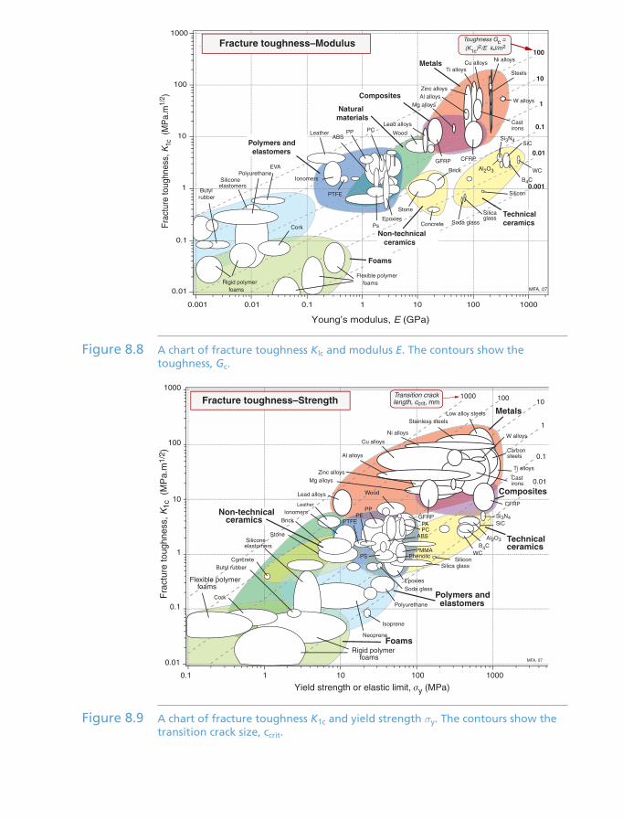
100
10
1
0.1
0.01
Young’s modulus, E (GPa)
Frac
ture
toug
hnes
s, K
1c (
MP
a.m
1/2 )
0.001 0.01 0.1 1 10 100 1000
0.01
0.1
1
10
100
1000
Polymers and elastomers
Metals
Technicalceramics
Composites
Natural materials
Lead alloys
W alloys
SteelsTi alloys
Mg alloys
CFRPGFRP
Al alloys
Rigid polymer foams
Flexible polymer foams
Ni alloysCu alloys
Zinc alloys
Ps
PTFE
PC
Cork
Wood
Butyl rubber
Silicone elastomers
Concrete
Al2O3
SiCSi3N4
Fracture toughness–Modulus
B4C
PP
EVAPolyurethane
Leather
Non-technical ceramics
Cast irons
WC
Soda glass
Silica glass
Silicon
Stone
Brick
ABS
Epoxies
Ionomers
MFA, 07
Toughness Gc =
(K1c)2/E kJ/m2
Foams
0.001
Figure 8.8 A chart of fracture toughness Klc and modulus E. The contours show thetoughness, Gc.
Yield strength or elastic limit, σy (MPa)
Fra
ctur
e to
ughn
ess,
K1c
(M
Pa.
m1/
2 )
0.1 1 10 100 1000
0.01
0.1
1
10
100
1000100 10
1
0.1
0.01
1000Transition cracklength, ccrit, mm
Non-technical ceramics
Foams
Polymers and elastomers
Metals
Technicalceramics
CompositesLead alloys
W alloys
Stainless steels
Ti alloys
Mg alloys
CFRP
GFRP
Al alloys
Rigid polymer foams
Flexible polymer foams
Ni alloys
Cu alloys
Zinc alloys
PMMA
Cork
Wood
Butyl rubber
Silicone elastomers
Concrete
Al2O3
SiCSi3N4
Fracture toughness–Strength
B4C
Neoprene
Isoprene
Leather
Castirons
WC
Soda glass
Silica glassSilicon
Stone
Brick
ABS
Epoxies
Ionomers
Low alloy steels
Carbon steels
Polyurethane
PAPC
PEPTFE
PS
PP
Phenolic
MFA, 07
Figure 8.9 A chart of fracture toughness K1c and yield strength σy. The contours show thetransition crack size, ccrit.
Ch08-H8391.qxd 1/17/07 10:45 AM Page 173

them on a property chart. Metals are both strong and tough—that is why theyhave become the workhorse materials of mechanical and structural engineering.
The stress at which fracture occurs depends on both K1c and the crack lengthc (equation (8.12)). The transition crack length ccrit at which ductile behavior isreplaced by brittle is given by equation (8.13). It is plotted on the chart as bro-ken lines labeled ‘Transition crack length’. The values vary enormously, fromnear-atomic dimensions for brittle ceramics and glasses to almost a meter forthe most ductile of metals like copper or lead. Materials towards the bottomright have high strength and low toughness; they fracture before they yield.Those towards the top left do the opposite: they yield before they fracture.
The diagram has application in selecting materials for the safe design of load-bearing structures (Chapter 10). The strength–fracture toughness chart is also useful for assessing the influence of composition and processing on properties.
8.5 Drilling down: the origins of toughness
Surface energyThe surface energy of a solid is the energy it costs to make it. It is an energy perunit area, units J/m2. Think of taking a 1 m cube of material and cutting it inhalf to make two new surfaces, one above and one below, as in Figure 8.10. Todo so we have to provide the cohesive energy associated with the bonds thatpreviously connected across the cut. The atoms are bonded on all sides so thesurface atoms lose one-sixth of their bonds when the cut is made. This meansthat we have to provide one-sixth of the cohesive energy Hc (an energy per unit
174 Chapter 8 Fracture and fracture toughness
Unit cube1 m3
Cut hereNew surface,energy γ/m2
New surface
of bondsbroken
16
Figure 8.10 When new surface is created as here, atomic bonds are broken, requiring somefraction of the cohesive energy, Hc.
Ch08-H8391.qxd 1/17/07 10:45 AM Page 174
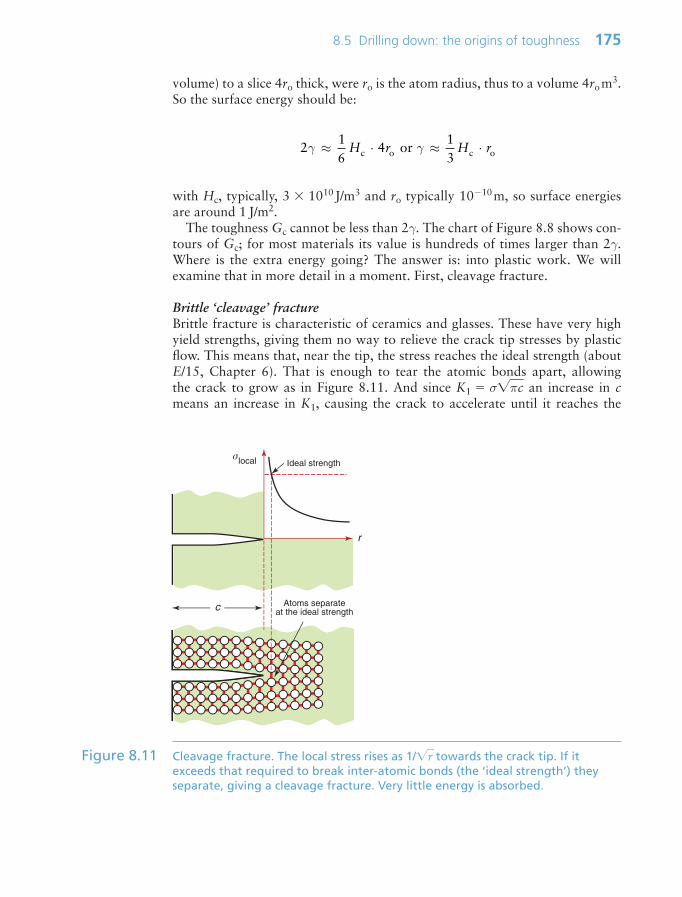
volume) to a slice 4ro thick, were ro is the atom radius, thus to a volume 4rom3.So the surface energy should be:
with Hc, typically, 3 1010J/m3 and ro typically 1010m, so surface energiesare around 1 J/m2.
The toughness Gc cannot be less than 2γ. The chart of Figure 8.8 shows con-tours of Gc; for most materials its value is hundreds of times larger than 2γ.Where is the extra energy going? The answer is: into plastic work. We willexamine that in more detail in a moment. First, cleavage fracture.
Brittle ‘cleavage’ fractureBrittle fracture is characteristic of ceramics and glasses. These have very highyield strengths, giving them no way to relieve the crack tip stresses by plasticflow. This means that, near the tip, the stress reaches the ideal strength (aboutE/15, Chapter 6). That is enough to tear the atomic bonds apart, allowing the crack to grow as in Figure 8.11. And since K1 σπc an increase in cmeans an increase in K1, causing the crack to accelerate until it reaches the
216
4 or13c o c oγ γ≈ ⋅ ≈ ⋅H r H r
8.5 Drilling down: the origins of toughness 175
c
r
σlocal Ideal strength
Atoms separateat the ideal strength
Figure 8.11 Cleavage fracture. The local stress rises as 1/r towards the crack tip. If itexceeds that required to break inter-atomic bonds (the ‘ideal strength’) theyseparate, giving a cleavage fracture. Very little energy is absorbed.
Ch08-H8391.qxd 1/17/07 10:45 AM Page 175

speed of sound—that is why brittle materials fail with a bang. Some polymersare brittle, particularly the amorphous ones. The crack tip stresses unzip theweak van der Waals bonds between the molecules.
Tough ‘ductile’ fractureTo understand how cracks propagate in ductile materials, think first of pullinga sample with no crack, as in Figure 8.12. Ductile metals deform plasticallywhen loaded above their yield strength, work hardening until the tensilestrength is reached. Thereafter, they weaken and fail. What causes the weaken-ing? If ultra-pure, the metal may simply thin down until the cross-section goesto zero. Engineering alloys are not ultra-pure; almost all contain inclusions—small, hard particles of oxides, nitrides, sulfides and the like. As the material—here shown as a test specimen—is stretched, it deforms at first in a uniform way,building up stress at the inclusions, which act as stress concentrations. Theseeither separate from the matrix or fracture, nucleating tiny holes. The holesgrow as strain increases, linking and weakening the part of the specimen in whichthey are most numerous until they finally coalesce to give a ductile fracture.Many polymers, too, are ductile. They don’t usually contain inclusions becauseof the way in which they are made. But when stretched they craze—tiny cracksopen up in the most stretched regions, whitening them if the polymer is trans-parent, simply because the Van der Waals bonds that link their long chains toeach other are weak and pull apart easily. The details differ but the results arethe same: the crazes nucleate, grow and link to give a ductile fracture.
Return now to the cracked sample, shown in Figure 8.13. The stress still risesas 1/r as the crack tip is approached, but at the point that it exceeds the yieldstrength σy the material yields and a plastic zone develops. Within the plastic
176 Chapter 8 Fracture and fracture toughness
(d)(b) (c)
(a)
Inclusions Plasticity VoidsVoid
linkage
FF
F
Figure 8.12 Ductile fracture. Plasticity, shown in red, concentrates stress on inclusions thatfracture or separate from the matrix, nucleating voids that grow and link,ultimately causing fracture.
Ch08-H8391.qxd 1/17/07 10:45 AM Page 176

zone the same sequence as that of Figure 8.12 takes place: voids nucleate, growand link to give a ductile fracture. The crack advances and the process repeatsitself. The plasticity blunts the crack and the stress-concentrating effect of ablunt crack is less severe than that of a sharp one, so that at the crack tip itselfthe stress is just sufficient to keep plastically deforming the material there. Thisplastic deformation absorbs energy, increasing the toughness Gc.
The ductile-to-brittle transitionA cleavage fracture is much more dangerous than one that is ductile: it occurswithout warning or any prior plastic deformation. At low temperatures somemetals and all polymers become brittle and the fracture mode switches fromone that is ductile to one of cleavage—in fact only those metals with an fccstructure (copper, aluminum, nickel and stainless steel, for example) remainductile to the lowest temperatures. All others have yield strengths that increaseas the temperature falls, with the result that the plastic zone at any crack theycontain shrinks until it becomes so small that the fracture mode switches, giv-ing a ductile-to-brittle transition. For some steels that transition temperature isas high as 0°C (though for most it is considerably lower), with the result thatsteel ships, bridges and oil rigs are more likely to fail in winter than in summer.Polymers, too, have a ductile-to-brittle transition, a consideration in selectingthose that are to be used in freezers and fridges.
8.5 Drilling down: the origins of toughness 177
c
r
σlocal
Yield strength σy
Plastic zone Inclusions
ry
Figure 8.13 If the material is ductile a plastic zone forms at the crack tip. Within it voidsnucleate, grow and link, advancing the crack in a ductile mode, absorbingenergy in the process.
Ch08-H8391.qxd 1/17/07 10:45 AM Page 177

Embrittlement of other kindsChange of temperature can lead to brittleness; so, too, can chemical segrega-tion. When metals solidify, the grains start as tiny solid crystals suspended inthe melt, and grow outwards until they impinge to form grain boundaries. Theboundaries, being the last bit to solidify, end up as the repository for the impu-rities in the alloy. This grain boundary segregation can create a network of low-toughness paths through the material so that, although the bulk of the grains istough, the material as a whole fails by brittle intergranular fracture (Figure8.14). The locally different chemistry of grain boundaries causes other prob-lems, such as corrosion (Chapter 17)—one way in which cracks can appear ininitially defect-free components.
8.6 Manipulating properties: the strength–toughness trade-off
MetalsIt is not easy to make materials that are both strong and tough. The energyabsorbed by a crack when it advances, giving toughness, derives from the defor-mation that occurs in the plastic zone at its tip. Equation (8.11) showed thatincreasing the yield strength causes the zone to shrink and the smaller thezone, the smaller the toughness. Figure 8.15 shows strength and toughness forwrought and cast aluminum alloys, indicating the strengthening mechanisms.All the alloys have a higher strength and lower toughness than pure aluminum.The wrought alloys show a slight drop in toughness with increasing strength; forthe cast alloys the drop is much larger because of intergranular fracture.
Separation within the plastic zone, allowing crack advance, results from thegrowth of voids that nucleate at inclusions (Figure 8.13). Toughness isincreased with no loss of strength if the inclusions are removed, delaying thenucleation of the voids. ‘Clean’ steels, superalloys and aluminum alloys, made
178 Chapter 8 Fracture and fracture toughness
Intergranularcrack
Segregationat boundaries
Grains
Figure 8.14 Chemical segregation can cause brittle intergranular cracking.
Ch08-H8391.qxd 1/17/07 10:45 AM Page 178

8.6 Manipulating properties: the strength–toughness trade-off 179
Fra
ctur
e to
ughn
ess
K1c
(M
Pa.
m1/
2 )
20
30
70
100
10
50
Yield strength σy (MPa)10003001003010
Castingalloys
Wrought alloys
7075 T6
6082 T62024 T6
Precipitatestrengthened
Solid solutionstrengthened
1050, soft
1050, workhardened
Pure Al
Work hardening
5083
A201
A356
S413
Aluminum alloys
Figure 8.15 The strength and toughness of wrought and cast aluminum alloys.
by filtering the molten metal before casting, have significantly higher toughnessthan those made by conventional casting methods.
Polymers and compositesThe microstructures and properties of polymers are manipulated by cross-link-ing and by adjusting the molecular weight and degree of crystallinity. Figures8.8 and 8.9 showed that the strengths of polymers span around a factor of 5,while fracture toughnesses spans a factor of 20. More dramatic changes arepossible by blending, by adding fillers and by reinforcement with chopped orcontinuous fibers to form composites. Figure 8.16 shows how these influencethe modulus E and fracture toughness K1c of polypropylene (PP). Blending orco-polymerization with elastomers such as EPR or EDPM (‘impact modifiers’)reduces the modulus but increases the fracture toughness K1c and toughness Gc.Filling with cheap powdered glass, talc or calcium carbonate more than dou-bles the modulus, but at the expense of some loss of toughness.
Reinforcement with glass or carbon fibers most effectively increases bothmodulus and fracture toughness K1c, and in the case of glass, the toughness Gcas well. How is it that a relatively brittle polymer (K1c 3MPa.m1/2) mixed witheven more brittle fibers (glass K1c 0.8 MPa.m1/2) can give a composite K1c ashigh as 10 MPa.m1/2? The answer is illustrated in Figure 8.17. The fine fiberscontain only tiny flaws and consequently have high strengths. When a crackgrows in the matrix, the fibers remain intact and bridge the crack. This promotes
Ch08-H8391.qxd 1/17/07 10:45 AM Page 179

multiple cracking—each contributing its own energy and thereby raising theoverall dissipation. When the fibers do break, the breaks are statistically dis-tributed, leaving ligaments of fiber buried in the matrix. Fiber pull-out, as thecracks open up, dissipates more energy by friction. Composites are processed tocontrol adhesion between the fibers and the matrix to maximize the toughen-ing by these mechanisms.
180 Chapter 8 Fracture and fracture toughness
Matrix
Fibers
Crack
Fiber fracture
Debondingand pull-out
Frictionalshear force
Figure 8.17 Toughening by fibers. The pull-out force opposes the opening of the crack.
Young’s modulus E (GPa)0.2 0.5 1 2 5 10 20
Fra
ctur
e to
ughn
ess
K1c
(M
Pa.
m1/
2 )
0.5
1
2
5
10
PP homopolymer
PP co-polymer
PP with EPR
Fillers
Impact modifiers
Carbon fibers
Glass fibers
Polypropylene
10% CaCO3
20% CaCO3
40% CaCO3
40% Talc
40% long glass fiber
20% longglass fiber
30% PAN carbon fiber
Gc = 1 kJ/m2
Gc = 10 kJ/m2
Figure 8.16 The strength and toughness of polypropylene, showing the effect of fillers,impact modifiers and fibers.
Ch08-H8391.qxd 1/17/07 10:45 AM Page 180
8.7 Summary and conclusions
Toughness is the resistance of a material to the propagation of a crack. Toughmaterials are forgiving: they tolerate the presence of cracks, they absorb impactwithout shattering and, if overloaded, they yield rather than fracture. The dom-inance of steel as a structural material derives from its unbeatable combinationof low cost, high stiffness and strength, and high toughness.
Toughness is properly measured by loading a pre-cracked sample with one ofa number of standard geometries, measuring the load at which the crack firstpropagates. From this is calculated the fracture toughness, K1c, as the value ofthe stress intensity, K1, at which the crack advances. Values of K1c above about15 MPa.m1/2 are desirable for damage-tolerant design—design immune to thepresence of small cracks. The charts of Figures 8.8 and 8.9 show that most met-als and fiber-reinforced composites meet this criterion, but polymers andceramics fall below it. We shall see in Chapter 10 that some designs require ahigh value not of K1c but of the toughness Gc K2
1c/E, also shown in the chartof Figure 8.8. Polymers do well by this criterion and it is in applications thatrequire it that they become a good choice. Ceramics are poor by this criteriontoo, making design with them much more difficult.
High toughness means that crack advance absorbs energy. It does so in theplastic zone that forms at the crack tip; the larger this becomes, the higher is thefracture toughness. As the material within the plastic zone deforms, voidsnucleate at inclusions and link, advancing the crack; the cleaner the material,the fewer are the inclusions, contributing further to high toughness. The higherthe yield strength, the smaller is the zone until, in ceramics, which have veryhigh yield strengths, the zone becomes vanishingly small, the stresses approachthe ideal strength and the material fails by brittle cleavage fracture.
This is the background we need for design. That comes in Chapter 10, afterwe have examined fracture under cyclic loads.
8.8 Further reading
Broek, D. (1981) Elementary Engineering Fracture Mechanics, 3rd edition, MartinusNijhoff, Boston, USA. ISBN 90-247-2580-1. (A standard, well-documented, intro-duction to the intricacies of fracture mechanics.)
Ewalds, H.L. and Wanhill, R.J.H. (1984) Fracture Mechanics, Edward Arnold, London,UK. ISBN 0-7131-3515-8. (An introduction to fracture mechanics and testing forboth static and cyclic loading.)
Hertzberg, R.W. (1989) Deformation and Fracture of Engineering Materials, 3rd edi-tion, Wiley, New York, USA. ISBN 0-471-63589-8. (A readable and detailed coverageof deformation, fracture and fatigue.)
Kinloch, A.J. and Young, R.J. (1983) Fracture Behavior of Polymers, Elsevier AppliedScience, London, UK. ISBN 0-85334-186-9. (An introduction both to fracturemechanics as it is applied to polymeric systems and to the fracture behavior of differ-ent classes of polymers and composites.)
8.8 Further reading 181
Ch08-H8391.qxd 1/17/07 10:45 AM Page 181

Knott, J.F. (1973) The Mechanics of Fracture, Butterworths, London, UK. ISBN 0-408-70529-9. (One of the first texts to present a systematic development of the mechanicsof fracture; dated, but still a good introduction.)
Tada, H., Paris, G. and Irwin, G.R. (2000) The Stress Analysis of Cracks Handbook,3rd edition. ISBN 1-86058-304-0. (Here we have another ‘Yellow Pages’, like Roarkfor stress analysis of uncracked bodies—this time of stress intensity factors for a greatrange of geometries and modes of loading.)
8.9 Exercises
182 Chapter 8 Fracture and fracture toughness
Exercise E8.1 What is meant by toughness? How does it differ from strength?
Exercise E8.2 Why does a plastic zone form at the tip of a crack when the cracked body isloaded in tension?
Exercise E8.3 Why is there a transition from ductile to brittle behavior at a transition cracklength, ccrit?
Exercise E8.4 A tensile sample of width 10 mm contains an internal crack of length0.3 mm. When loaded in tension the crack suddenly propagates when thestress reaches 450 MPa. What is the fracture toughness K1c of the material ofthe sample? If the material has a modulus E of 200 GPa, what is its tough-ness Gc? (Assume Y 1).
Exercise E8.5 Use the K1c–E chart of Figure 8.8 to establish:
• Whether CFRP has higher fracture toughness K1c than aluminum alloys?• Whether polypropylene (PP) has a higher toughness Gc than aluminum
alloys.• Whether polycarbonate (PC) has a higher fracture toughness K1c than
glass.
Exercise E8.6 Find epoxy, soda glass and GFRP (epoxy reinforced with glass fibers) on thechart of Figure 8.8 and read off an approximate mean value for the tough-ness Gc for each. Explain how it is that the toughness of the GFRP is so muchlarger than that of either of its components.
Exercise E8.7 Use the chart of Figure 8.8 to compare the fracture toughness, K1c, of the twocomposites GFRP and CFRP. Do the same for their toughness, Gc. What dothe values suggest about applications they might best fill?
Exercise E8.8 Use the K1c–σy chart of Figure 8.9 to find:
• The range of transition crack sizes for stainless steel.• The range of transition crack sizes for polycarbonate (PC).• The range of transition crack sizes for silicon nitride (Si3N4).
Ch08-H8391.qxd 1/17/07 10:45 AM Page 182

8.11 Exploring the science with CES Elements 183
Exercise E8.9 Make a bar chart with σf K1c/πc for an internal crack of length2c 1 mm plotted on the y-axis (use the ‘Advanced’ facility to form thefunction
Fracture toughness /( (3.142 0.0005)^0.5).Which materials have the highest values? Add an axis of density, ρ. Use thenew chart to find the two materials with highest values of σf /ρ.
Exercise E8.10 Suppose that the resolution limit of the non-destructive testing facility avail-able to you is 1 mm, meaning that it can detect cracks of this length or larger.You are asked to explore which materials will tolerate cracks equal to orsmaller than this without brittle fracture. Make a bar chart withσf K1c/πc for an internal crack of length 2c 1 mm plotted on the y-axis, as in the previous exercise. Add yield strength, σy, on the x-axis. Thematerial will fracture in tension if σf σy, and it will yield, despite beingcracked, if σf σy. Plot either on a print out of the chart or in CES (using theline selection tool) a line of slope 1 along which σf σy. All the materialsabove the line will yield, all those below will fracture. Do age-hardened alu-minum alloys lie above the line? Does CFRP?
Exercise E8.11 Find data for PVCs in the Level 3 database and make a plot like that ofFigure 8.16 showing how fillers, blending and fibers influence modulus andtoughness.
Exercise E8.12 Exploring the origins of surface energy, γ J/m2. The toughness, Gc, cannot beless than 2γ because two new surfaces are created when a material is frac-tured. What determines γ and how big is it? The text explained how bondsare broken and atoms separated when a new surface is created. It was shownin Section 8.4 that
where Hc is the cohesive energy in J/m3 and ro is the atomic radius in m. Toconvert Hc in kJ/mol (as it is in the database) into these units, multiply it by
≈ ⋅13 c oH r
8.10 Exploring design with CES (use the Level 2 database unlessotherwise stated)
8.11 Exploring the science with CES Elements
Ch08-H8391.qxd 1/17/07 10:45 AM Page 183

184 Chapter 8 Fracture and fracture toughness
106/ molar volume and to convert ro from nm into m multiply by 109. Allthis can be done using the ‘Advanced’ facility in the axis-choice dialog box.
Make a chart with γ calculated in this way on the x-axis and the mea-sured value, ‘Surface energy, solid’ on the y-axis, and see how good theagreement is.
Exercise E8.13 If you pull on an atomic bond, it breaks completely at a strain of about 0.1.If the atom spacing is ao, then breaking it requires a displacement δ 0.1aoand doing so creates two new surfaces, each of area a2
o. If the bond stiffnessis S, then the work done to stretch the bonds to breaking point, and hence tocreate the new surfaces, per unit area, is
(using equation (4.17) for S), where ro is the atomic radius. Use the CESElements database to explore whether real surface energies can be explained inthis way. (Watch out for the units.)
Exercise E8.14 Observe the general magnitudes of surface energies γ: they are about1.5 J/m2. Thus, the minimum value for Gc should be about 2γ or 3 J/m2.Return to the CES Edu Level 3 database and find the material with the low-est value of Gc, which you can calculate as Klc
2/E. Is it comparable with 2γ?Limit the selection to metals and alloys, polymers, technical ceramics andglasses only, using a ‘Tree’ stage (materials such as foam have artificially lowvalues of Gc because they are mostly air).
21 1
2 201
10o2
oo ≈
⎛
⎝⎜⎜⎜
⎞
⎠⎟⎟⎟⎟a
SEa
Er
Ch08-H8391.qxd 1/17/07 10:45 AM Page 184

Chapter 9Shake, rattle and roll: cyclicloading, damage and failure
Chapter contents
9.1 Introduction and synopsis 1869.2 Vibration and resonance: the
damping coefficient 1869.3 Fatigue 1879.4 Charts for endurance limit 1949.5 Drilling down: the origins of
damping and fatigue 1959.6 Manipulating resistance to fatigue 1969.7 Summary and conclusions 1989.8 Further reading 1999.9 Exercises 1999.10 Exploring design with CES 201
A bolt that has failed by fatigue. The fatigue crackinitiated at the root of a thread, which acts as anotch, concentrating stress. (Image courtesy Bolt
Science (www.Boltscience.com))
Ch09-H8391.qxd 1/16/07 6:04 PM Page 185

186 Chapter 9 Shake, rattle and roll: cyclic loading, damage and failure
9.1 Introduction and synopsis
German engineering was not always what it is today. The rapidly expandingrailway system of the mid-19th century was plagued, in Germany and else-where, by accidents, many catastrophic, caused by the failure of the axles of thecoaches. The engineer August Wöhler1 was drafted in to do something about it.It was his systematic tests that first established the characteristics of what wenow call fatigue.
Repetition is tiring, the cause of many human mistakes and accidents.Materials, too, grow tired if repeatedly stressed, with failure as a consequence.This chapter is about the energy that is dissipated, and the damage and failurethat can result, when materials are loaded in a cyclic, repetitive way. Even whenthe amplitude of the cycles is very small, some energy dissipation or dampingoccurs. Larger amplitudes cause the slow accumulation of damage, a little oneach cycle, until a critical level is reached at which a crack forms. Continuedcycling causes the crack to grow until the component suddenly fails. Fatiguefailure is insidious—there is little sign that anything is happening until, bang, itdoes. So when the clip breaks off your pen or your office chair collapses, it isprobably fatigue that is responsible (cover picture).
We start with cyclic loading at very small amplitudes and the energy loss ordamping that goes with it. We then turn to the accumulation of damage andcracking that is associated with fatigue loading proper.
9.2 Vibration and resonance: the damping coefficient
Bells, traditionally, are made of bronze. They can be (and sometimes are) madeof glass, and they could (if you could afford it) be made of silicon carbide.Metals, glasses and ceramics all, under the right circumstances, have low mate-rial damping or ‘internal friction’, an important material property when struc-tures vibrate. By contrast, leather, wood (particularly when green or wet) andmost foams, elastomers and polymers have high damping, useful when youwant to kill vibration.
We are speaking here of elastic response. Until now we have thought of the elas-tic part of the stress–strain curve as linear and completely reversible so that theelastic energy stored on loading is completely recovered when the load is removed.No material is so perfect—some energy is always lost in a load–unload cycle. Ifyou load just once, you might not notice the loss, but in vibration at, say, acousticfrequencies, the material is loaded between 20 and 20 000 times per second, as instress cycle (a) of Figure 9.1. Then the energy loss becomes only too obvious.
1 August Wöhler (1819–1914), German engineer, and from 1854 to 1889 Director of thePrussian Imperial Railways. It was Wöhler’s systematic studies of metal fatigue that firstgave insight into design methods to prevent it.
Ch09-H8391.qxd 1/16/07 6:04 PM Page 186

9.3 Fatigue 187
The mechanical loss coefficient or damping coefficient, η (a dimensionlessquantity), measures the degree to which a material dissipates vibrational energy.If an elastic material is loaded, energy is stored (Chapter 5). If it is unloaded, theenergy is returned—it is how springs work. But materials have ways of cheatingon this: the amount of energy returned is slightly less. The difference is called theloss coefficient, η. It is the fraction of the stored elastic energy that is not returnedon unloading. If you seek materials for bells, you choose those with low η, butif you want to damp vibration, then you choose those with high.
9.3 Fatigue
The problem of fatigueLow-amplitude vibration causes no permanent damage in materials. Increasethe amplitude, however, and the material starts to suffer fatigue. You will, atsome time or other, have used fatigue to flex the lid off a sardine can or to breakan out-of-date credit card in two. The cyclic stress hardens the material andcauses damage in the form of dislocation tangles to accumulate, from which acrack nucleates and grows until it reaches the critical size for fracture. Anythingwhich is repeatedly loaded (like an oil rig loaded by the waves or a pressure ves-sel that undergoes pressure cycles), or rotates under load (like an axle), orreciprocates under load (like an automobile connecting rod), or vibrates (likethe rotor of a helicopter) is a potential candidate for fatigue failure.
Figure 9.2 shows in a schematic way how the stress on the underside of anaircraft wing might vary during a typical flight, introducing some important
Time, tS
tres
s, σ
σts
−σts
σy
−σy
(a)
(b)
(c)
Figure 9.1 Cyclic loading. (a) Very low amplitude acoustic vibration. (b) High-cycle fatigue:cycling well below general yield, σy. (c) Low cycle fatigue: cycling above generalyield (but below the tensile strength σts).
Ch09-H8391.qxd 1/16/07 6:04 PM Page 187

practicalities of fatigue. First, the amplitude of the stress varies as the aircrafttakes off, cruises at altitude, bumps its way through turbulence and finallylands. Second, on the ground the weight of the engines (and the wings them-selves) bends them downwards, putting the underside in compression. Once inflight, aerodynamic lift bends them upwards, putting the underside in tension.The amplitude of the stress cycles and their mean values change during flight.Fatigue failure depends on both. And of course it depends on the total numberof cycles. Aircraft wings bend to and fro at a frequency of a few hertz. In atrans-Atlantic flight, tens of thousands of loading cycles take place; in the life-time of the aircraft, it is millions. For this reason, fatigue testing needs to applytens of millions of fatigue cycles to provide meaningful design data.
The food can and credit card are examples of low-cycle fatigue, meaning thatthe component only survives for a small number of cycles. It is typical of cyclingat stresses above the yield stress, σy, like that shown in Figure 9.1(c). More sig-nificant in engineering terms is high-cycle fatigue: here the stresses remain gen-erally elastic and may be well below σy, as in cycle (b) of Figure 9.1; cracksnonetheless develop and cause failure, albeit taking many more cycles to do so,as in Wöhler’s railway axles.
In both cases we are dealing with components that are initially undamaged,containing no cracks. In these cases, most of the fatigue life is spent generatingthe crack. Its growth to failure occurs only at the end. We call this initiation-controlled fatigue. Some structures contain cracks right from the word go, or areso safety-critical (like aircraft) that they are assumed to have small cracks. Thereis then no initiation stage—the crack is already there—and the fatigue life ispropagation controlled, i.e. it depends on the rate at which the crack grows. Adifferent approach to design is then called for—we return to this below.
188 Chapter 9 Shake, rattle and roll: cyclic loading, damage and failure
Str
ess,
σ
Taxiing Taxiing
Cruising Turbulence
LandingTake-off
Time t
Figure 9.2 Schematic of stress cycling on the underside of a wing during flight.
Ch09-H8391.qxd 1/16/07 6:04 PM Page 188

High-cycle fatigue and the S–N curveFigure 9.3 shows how fatigue characteristics are measured and plotted. A sam-ple is cyclically stressed with amplitude ∆σ/2 about a mean value σm, and thenumber of cycles to cause fracture is recorded. The data are presented as ∆σ –Nf (‘S–N’) curves, where ∆σ is the peak-to-peak range over which the stressvaries and Nf is the number of cycles to failure. Most tests use a sinusoidallyvarying stress with an amplitude σa of
(9.1)
and a mean stress σm of
(9.2)
all defined in the figure. Fatigue data are usually reported for a specified R-value:
(9.3)
An R-value of 1 means that the mean stress is zero; an R-value of 0 means thestress cycles from 0 to σmax. For many materials there exists a fatigue or
R σσ
min
max
σσ σ
mmax min
2
σσ σ σ
amax min
∆2 2
9.3 Fatigue 189
Str
ess
am
plitu
de σ
a
Cycles to failure, Nf (log scale)
σts
σe
1 108
107
cycles
∆σ
Endurance limit
∆σ
σmax
σminTime
σmσa
10 102 103 104 105 106 107
Figure 9.3 Fatigue strength at 107 cycles, the endurance limit, σe.
Ch09-H8391.qxd 1/16/07 6:04 PM Page 189

endurance limit, σe (units: MPa). It is the stress amplitude σa, about zero meanstress, below which fracture does not occur at all, or occurs only after a very largenumber (Nf 107) cycles. Design against high-cycle fatigue is therefore verysimilar to strength-limited design, but with the maximum stresses limited bythe endurance limit σe rather than the yield stress σy.
Experiments show that the high-cycle fatigue life is approximately related tothe stress range by what is called Basquin’s law:
∆σ Nbf C1 (9.4)
where b and C1 are constants; the value of b is small, typically 0.07 and 0.13.Dividing ∆σ by the modulus E gives the strain range ∆ε (since the sample iselastic):
(9.5)
or, taking logs,
Log(∆ε) b Log(Nf) Log(C1/E)
This is plotted in Figure 9.4, giving the right-hand, high-cycle fatigue part ofthe curve with a slope of b.
∆∆
εσ
E
C E
Nb1 /
f
190 Chapter 9 Shake, rattle and roll: cyclic loading, damage and failure
Log
(Str
ain
ampl
itude
, ∆ε)
Log (cycles to failure, N f )
Coffinslope-c
Basquinslope-b
Low-cyclefatigue
High-cyclefatigue
Bulk of sampleplastic
Bulk of sampleelastic
1 108102 104 106 1010
E∆ε = ∆σ
Figure 9.4 The low- and high-cycle regimes of fatigue and their empirical description offatigue.
Ch09-H8391.qxd 1/16/07 6:04 PM Page 190

Low-cycle fatigueIn low-cycle fatigue the peak stress exceeds yield, so at least initially (beforework hardening raises the strength), the entire sample is plastic. Basquin is nohelp to us here; we need another empirical law, this time that of Dr Lou Coffin:
(9.6)
where ∆εpl means the plastic strain range—the total strain minus the (usuallysmall) elastic part. For our purposes we can neglect that distinction and plot itin Figure 9.4 as well, giving the left-hand branch. Coffin’s exponent, c, is muchlarger than Basquin’s; typically it is 0.5.
These laws adequately describe the fatigue failure of uncracked componentscycled at constant amplitude about a mean stress of zero. But as we saw, realloading histories are often much more complicated (Figure 9.2). How do wemake some allowance for variations in mean stress and stress range? Here weneed yet more empirical laws, courtesy this time of Goodman and Miner.Goodman’s rule relates the stress range ∆σσm for failure under a mean stress σmto that for failure at zero mean stress ∆σσo:
(9.7)
where σts is the tensile stress, giving a correction to the stress range. Increasingσm causes a small stress range ∆σσm to be as damaging as a larger ∆σσo appliedwith zero mean (Figure 9.5(a)). The corrected stress range may then be pluggedinto Basquin’s law.
∆ ∆σ σσσσ σm
m
ts
0
1⎛
⎝⎜⎜⎜⎜
⎞
⎠⎟⎟⎟⎟⎟
∆εpl
f
C
Nc2
9.3 Fatigue 191
σmax
σmin
∆σσo
σmax
σmin
∆σσm
0
0
σm
σm= 0
∆σ2
∆σ3
∆σ1
(a) (b) Str
ess,
σ
Figure 9.5 (a) The endurance limit refers to a zero mean stress. Goodman’s law scales ofthe stress range to a mean stress σm. (b) When the cyclic stress amplitudechanges, the life is calculated using Miner’s cumulative damage rule.
Ch09-H8391.qxd 1/16/07 6:04 PM Page 191
The variable amplitude problem can be addressed approximately with Miner’srule of cumulative damage. Figure 9.5(b) shows an idealized loading history withthree stress amplitudes (all about zero mean). Basquin’s law gives the numberof cycles to failure if each amplitude was maintained throughout the life of thecomponent. So if N1 cycles are spent at stress amplitude ∆σ1 a fraction N1/Nf,1of the available life is used up, where Nf,1 is the number of cycles to failure atthat stress amplitude. Miner’s rule assumes that damage accumulates in thisway at each level of stress. Then failure will occur when the sum of the damagefractions reaches 1—that is, when
(9.8)
Goodman’s law and Miner’s rule are adequate for preliminary design, but theyare approximate; in safety-critical applications, tests replicating service con-ditions are essential. It is for this reason that new models of cars and trucks are driven over rough ‘durability tracks’ until they fail—it is a test of fatigueperformance.
The discussion so far has focused on initiation-controlled fatigue failure ofuncracked components. Now it is time to look at those containing cracks.
Fatigue loading of cracked componentsIn fabricating large structures like bridges, ships, oilrigs, pressure vessels andsteam turbines, cracks and other flaws cannot be avoided. Cracks in castingsappear because of differential shrinkage during solidification and entrapmentof oxide and other inclusions. Welding, a cheap, widely-used joining process,can introduce both cracks and internal stresses caused by the intense local heat-ing. If the cracks are sufficiently large that they can be found it may be possibleto repair them, but finding them is the problem. All non-destructive testing(NDT) methods for detecting cracks have a resolution limit; they cannot tell usthat there are no cracks, only that there are none longer than the resolutionlimit, clim. Thus, it is necessary to assume an initial crack exists and design thestructure to survive a given number of loadings. So how is the propagation ofa fatigue crack characterized?
Fatigue crack growth is studied by cyclically loading specimens containing asharp crack of length c like that shown in Figure 9.6. We define the cyclic stressintensity range, ∆K, using equation (8.4), as
(9.9)
The range ∆K increases with time under constant cyclic stress because the crackgrows in length: the growth per cycle, dc/dN, increases with ∆K in the wayshown in Figure 9.7. The rate is zero below a threshold cyclic stress intensity
∆ ∆K max min K K cσ π
N
Ni
ii
n
f,
1
1∑
192 Chapter 9 Shake, rattle and roll: cyclic loading, damage and failure
Ch09-H8391.qxd 1/16/07 6:04 PM Page 192

∆Kth, useful if you want to make sure it does not grow at all. Above it, there is asteady-state regime described by the Paris law:
(9.10)
where K and m are constants. At high ∆K the growth rate accelerates as themaximum applied K approaches the fracture toughness K1c. When it reachesK1c the sample fails in a single load cycle.
dd
cN
A Km ∆
9.3 Fatigue 193
Kmax
Kmin
∆K
0
Km
σmax
σmin
∆σ
0
σm
c
∆σ
∆σ
Sharp crack
Time
Time
Figure 9.6 Cyclic loading of a cracked component. A constant stress amplitude gives anincreasing amplitude of stress intensity, K c as the crack grows inlength.
Threshold ∆K
Fast fracture
dcdN
= A ∆Km
Log ∆K
Log
dc dN
Kmax = K1c
Figure 9.7 Crack growth during cyclic loading.
Ch09-H8391.qxd 1/16/07 6:04 PM Page 193

Safe design against fatigue failure in potentially cracked components meanscalculating the number of loading cycles that can safely be applied without thecrack growing to a dangerous length. We return to this in Chapter 10.
9.4 Charts for endurance limit
The most important single property characterizing fatigue strength is theendurance limit, σe, at 107 cycles and zero mean stress (an R-value of 1). Giventhis and the ability to scale it to correct for mean stress, and sum contributionswhen stress amplitude changes (equations (9.7) and (9.8)), enables design tocope with high-cycle fatigue.
Not surprisingly endurance limit and strength are related. The strongest corre-lation is with the tensile strength σts, shown in the chart of Figure 9.8. The datafor metals and polymers cluster around the line
σe 0.33 σts
shown on the chart. For ceramics and glasses
194 Chapter 9 Shake, rattle and roll: cyclic loading, damage and failure
Tensile strength σts (MPa)0.1 1 10 100 1000 10000
End
uran
ce li
mit
σ e (M
Pa)
0.1
1
10
100
1000
Non-technical ceramics
Foams
Polymers
Metals
Technicalceramics
Lead alloys
W alloys
Stainless steels
Ti alloys
Mg alloys CFRP
GFRP
Wrought Al alloys
Rigid polymer foams
Flexible polymer foams
Ni based superalloys
Cu alloys
Zinc alloys
PMMA
Butyl rubber
Concrete
Al2O3
Si3N4
Endurance limit–Strength
B4C
Neoprene
Isoprene
Cast irons
Soda glass
Silica glass
StoneBrick
Low alloy steels
Carbon steels
PET
PA
PC
PP
MFA, 07
Cast Al alloys
Al3N4
PE
DMC
ABS
Wood, -grainT
Wood, -grainll
Elastomers
σe = 0.33 σts
Figure 9.8 The endurance limit plotted against the tensile strength. Almost all materialsfail in fatigue at stresses well below the tensile strength.
Ch09-H8391.qxd 1/16/07 6:04 PM Page 194
σe 0.9 σts
In the next section we examine why.
9.5 Drilling down: the origins of damping and fatigue
Material damping: the mechanical loss coefficientThere are many mechanisms of material damping. Some are associated with aprocess that has a specific time constant; then the energy loss is centered about acharacteristic frequency. Others are frequency independent; they absorb energy atall frequencies. In metals a large part of the loss is caused by small-scale disloca-tion movement: it is high in soft metals like lead and pure aluminum. Heavilyalloyed metals like bronze and high-carbon steels have low loss because thesolute pins the dislocations; these are the materials for bells. Exceptionally highloss is found in some cast irons, in manganese–copper alloys and in magnesium,making them useful as materials to dampen vibration in machine tools and testrigs. Engineering ceramics have low damping because the dislocations in themare immobilized by the high lattice resistance (which is why they are hard).Porous ceramics, on the other hand, are filled with cracks, the surfaces of whichrub, dissipating energy, when the material is loaded. In polymers, chain seg-ments slide against each other when loaded; the relative motion dissipatesenergy. The ease with which they slide depends on the ratio of the temperatureT to the glass temperature, Tg, of the polymer. When T/Tg 1, the secondarybonds are ‘frozen’, the modulus is high and the damping is relatively low. WhenT/Tg 1, the secondary bonds have melted, allowing easy chain slippage; themodulus is low and the damping is high.
Fatigue damage and cracking
A perfectly smooth sample with no changes of section, and containing no inclu-sions, holes or cracks, would be immune to fatigue provided neither σmax norσmin exceeds its yield strength. But that is a vision of perfection that is unachiev-able. Blemishes, small as they are, can be deadly. Rivet holes, sharp changes insection, threads, notches and even surface roughness concentrate stress in the waydescribed in Chapter 7, Figure 7.7. Even though the general stress levels arebelow yield, the locally magnified stresses can lead to reversing plastic deforma-tion. Dislocation motion is limited to a small volume near the stress concentra-tion, but that is enough to cause damage that finally develops into a tiny crack.
In high-cycle fatigue, once a crack is present it propagates in the way shownin Figure 9.9(a). During the tensile part of a cycle a tiny plastic zone forms atthe crack tip, stretching it open and thereby creating a new surface. On the com-pressive part of the cycle the crack closes again and the newly formed surfacefolds forwards, advancing the crack. Repeated cycles make it inch forward,leaving tiny ripples on the crack face marking its position on each cycle. These
9.5 Drilling down: the origins of damping and fatigue 195
Ch09-H8391.qxd 1/16/07 6:04 PM Page 195
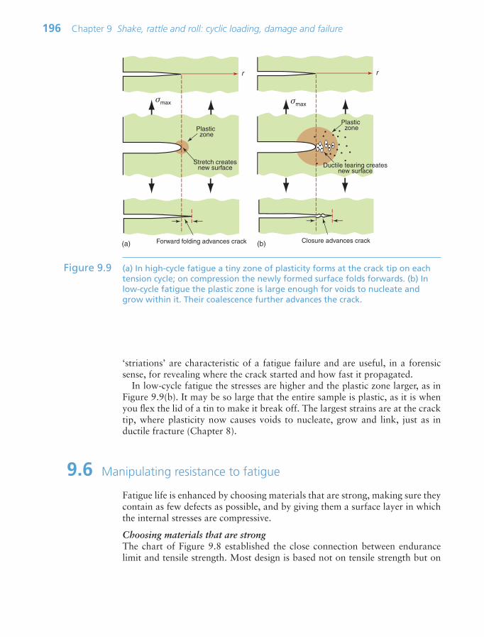
‘striations’ are characteristic of a fatigue failure and are useful, in a forensicsense, for revealing where the crack started and how fast it propagated.
In low-cycle fatigue the stresses are higher and the plastic zone larger, as inFigure 9.9(b). It may be so large that the entire sample is plastic, as it is whenyou flex the lid of a tin to make it break off. The largest strains are at the cracktip, where plasticity now causes voids to nucleate, grow and link, just as in ductile fracture (Chapter 8).
9.6 Manipulating resistance to fatigue
Fatigue life is enhanced by choosing materials that are strong, making sure theycontain as few defects as possible, and by giving them a surface layer in whichthe internal stresses are compressive.
Choosing materials that are strongThe chart of Figure 9.8 established the close connection between endurancelimit and tensile strength. Most design is based not on tensile strength but on
196 Chapter 9 Shake, rattle and roll: cyclic loading, damage and failure
r
Plastic zone
Stretch createsnew surface
Forward folding advances crack
r
Plastic zone
Ductile tearing createsnew surface
σmax
Closure advances crack
σmax
(a) (b)
Figure 9.9 (a) In high-cycle fatigue a tiny zone of plasticity forms at the crack tip on eachtension cycle; on compression the newly formed surface folds forwards. (b) Inlow-cycle fatigue the plastic zone is large enough for voids to nucleate andgrow within it. Their coalescence further advances the crack.
Ch09-H8391.qxd 1/16/07 6:04 PM Page 196

yield strength, and here the correlation is less strong. We define the fatigueratio, Fr, as
Figure 9.10 shows data for Fr for an age-hardening aluminum alloy and a lowalloy steel. Both can be heat-treated to increase their yield strength, and higherstrength invites higher design stresses. The figure, however, shows that the fatigueratio Fr falls as strength σy increases, meaning that the gain in endurance limit isconsiderably less than that in yield strength. In propagation-controlled fatigue,too, the combination of higher stress and lower fracture toughness implies thatsmaller crack sizes will propagate, causing failure (and the resolution of inspec-tion techniques may not be up to the job).
Making sure they contain as few defects as possibleMention has already been made of clean alloys—alloys with carefully controlledcompositions that are filtered when liquid to remove unwanted particles that, in the solid, can nucleate fatigue cracks. Non-destructive testing using X-rayimaging or ultrasonic sensing detects dangerous defects, allowing the part to be
Fre
y
Endurance limit
Yield strength
σσ
9.6 Manipulating resistance to fatigue 197
Yield strength, σy (MPa)50 100 200 500 1000 2000
Fat
igue
rat
io,
Fr
0.2
0.5
1
6061 Aluminum alloy AISI 4340 low-alloy steel
Soft (T4)condition
Hard(T6)condition
Tempered 650°C
Tempered 540°C
Tempered 315°C
Tempered 425°C
Tempered 205°C
AnnealedNormalized
Figure 9.10 The drop in fatigue ratio with increase in yield strength for an aluminum alloyand a steel, both of which can be treated to give a range of strengths.
Ch09-H8391.qxd 1/16/07 6:04 PM Page 197
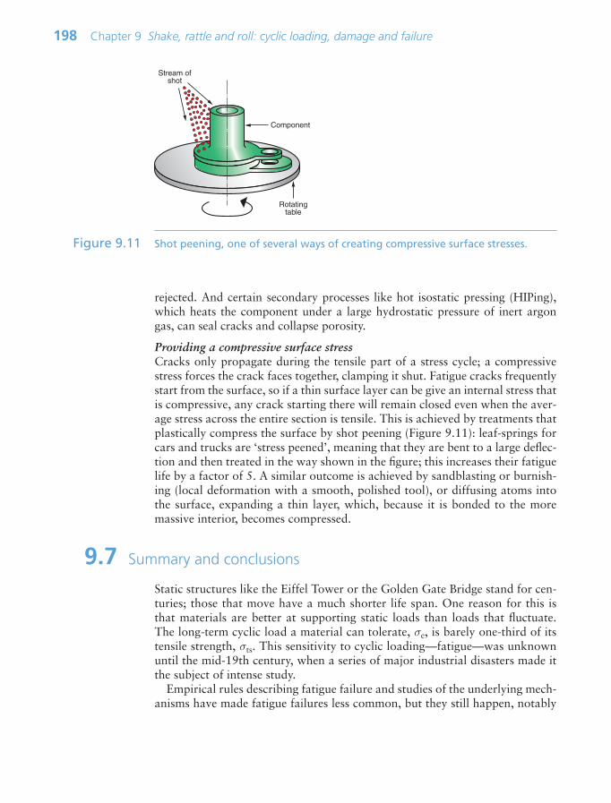
rejected. And certain secondary processes like hot isostatic pressing (HIPing),which heats the component under a large hydrostatic pressure of inert argongas, can seal cracks and collapse porosity.
Providing a compressive surface stressCracks only propagate during the tensile part of a stress cycle; a compressivestress forces the crack faces together, clamping it shut. Fatigue cracks frequentlystart from the surface, so if a thin surface layer can be give an internal stress thatis compressive, any crack starting there will remain closed even when the aver-age stress across the entire section is tensile. This is achieved by treatments thatplastically compress the surface by shot peening (Figure 9.11): leaf-springs forcars and trucks are ‘stress peened’, meaning that they are bent to a large deflec-tion and then treated in the way shown in the figure; this increases their fatiguelife by a factor of 5. A similar outcome is achieved by sandblasting or burnish-ing (local deformation with a smooth, polished tool), or diffusing atoms intothe surface, expanding a thin layer, which, because it is bonded to the moremassive interior, becomes compressed.
9.7 Summary and conclusions
Static structures like the Eiffel Tower or the Golden Gate Bridge stand for cen-turies; those that move have a much shorter life span. One reason for this isthat materials are better at supporting static loads than loads that fluctuate.The long-term cyclic load a material can tolerate, σe, is barely one-third of itstensile strength, σts. This sensitivity to cyclic loading—fatigue—was unknownuntil the mid-19th century, when a series of major industrial disasters made itthe subject of intense study.
Empirical rules describing fatigue failure and studies of the underlying mech-anisms have made fatigue failures less common, but they still happen, notably
198 Chapter 9 Shake, rattle and roll: cyclic loading, damage and failure
Stream ofshot
Component
Rotatingtable
Figure 9.11 Shot peening, one of several ways of creating compressive surface stresses.
Ch09-H8391.qxd 1/16/07 6:04 PM Page 198
in rail track, rolling stock, engines and airframes. It is now known that cyclingcauses damage that slowly accumulates until a crack nucleates, grows slowlyand suddenly runs unstably. This is pernicious behavior: the cracks are almostinvisible until final failure occurs without warning.
The rules and data for their empirical constants, described in this chapter, givea basis for design to avoid fatigue failure. The scientific studies provide insightthat guides the development of materials with greater resistance to fatigue fail-ure. Surface treatments to inhibit crack formation are now standard practice.We return to these in the next chapter, in which the focus is on design issues.
9.8 Further reading
Hertzberg, R.W. (1989) Deformation and Fracture of Engineering Materials, 3rd edition,Wiley, New York, USA. ISBN 0-471-63589-8. (A readable and detailed coverage ofdeformation, fracture and fatigue.)
Suresh, S. (1998) Fatigue of Materials, 2nd edition, Cambridge University Press, Cambridge,UK. ISBN 0-521-57847-7. (The place to start for an authoritative introduction to thematerials science of fatigue in both ductile and brittle materials.)
Tada, H., Paris, G. and Irwin, G.R. (2000) The Stress Analysis of Cracks Handbook, 3rdedition. ISBN 1-86058-304-0. (Here we have another ‘Yellow Pages’, like Roark forstress analysis of uncracked bodies—this time of stress intensity factors for a great rangeof geometries and modes of loading.)
9.9 Exercises 199
9.9 Exercises
Exercise E9.1 What is meant by the mechanical loss coefficient, η, of a material? Give exam-ples of designs in which it would play a role as a design-limiting property.
Exercise E9.2 What is meant by the endurance limit, σe, of a material?
Exercise E9.3 What is the fatigue ratio? If the tensile strength σts of an alloy is 900 MPa,what, roughly, would you expect its endurance limit σe to be?
Exercise E9.4 The figure shows an S–N curve for AISI 4340 steel, hardened to a tensilestrength of 1800 MPa.
• What is the endurance limit?• If cycled for 100 cycles at an amplitude of 1200 MPa and a zero mean
stress, will it fail?• If cycled for 100 000 cycles at an amplitude of 900 MPa and zero mean
stress, will it fail?• If cycled for 100 000 cycles at an amplitude of 800 MPa and a mean
stress of 300 MPa, will it fail?
Ch09-H8391.qxd 1/16/07 6:04 PM Page 199

200 Chapter 9 Shake, rattle and roll: cyclic loading, damage and failure
Exercise E9.5 The high-cycle fatigue life, Nf, of an aluminum alloy is described by Basquin’slaw:
(stress in MPa). How many cycles will the material tolerate at a stress ampli-tude σa of 70 MPa and zero mean stress? How will this change if the meanstress is 10 MPa? What if the mean stress is 10 MPa?
Exercise E9.6 The low-cycle fatigue of an aluminum alloy is described by Coffin’s law:
(stress in MPa). How many cycles will the material tolerate at a stress ampli-tude σa of 100 MPa?
Exercise E9.7 A material with a tensile stress σts 350 MPa is loaded cyclically about amean stress of 70 MPa. If the stress range that will cause fatigue fracture in105 cycles under zero mean stress is 60 MPa, what stress range about themean of 70 MPa will give the same life?
Exercise E9.8 A component made of the AISI 4340 steel with a tensile strength of 1800 MPaand the S–N curve shown in Exercise E9.4 is loaded cyclically between 0 and
∆σσ
2600
0 33
a fN( ) .
∆σσ
2480
0 12
a fN( ) .
Number of cycles to failure, Nf
400
500
600
700
800
900
1000
1100
1200
1300
1400
1500
103 104 105 106 107 108102
Str
ess
ampl
itude
, σa
(MP
a)
4340 Low-alloy steel,quenched and tempered 425°C Stress ratio R 1
Ch09-H8391.qxd 1/16/07 6:04 PM Page 200

9.9 Exercises 201
1200 MPa. What is the R-value and the mean stress, σm? Use Goodman’s ruleto find the equivalent stress amplitude for an R-value of 1, and read off thefatigue life from the S–N curve.
Exercise E9.9 A material has a threshold cyclic stress intensity ∆Kth of 2.5 MPam1/2. If it con-tains an internal crack of length 1 mm will it be safe (meaning, no failure) if sub-jected to continuous cyclic range of tensile stress ∆σ of 50 MPa?
Ch09-H8391.qxd 1/16/07 6:04 PM Page 201

202 Chapter 9 Shake, rattle and roll: cyclic loading, damage and failure
9.10 Exploring design with CES
Exercise E9.10 Make a bar chart of mechanical loss coefficient, η. Low loss materials are usedfor vibrating systems where damping is to be minimized—bells, high-frequencyrelays and resonant systems. High loss materials are used when damping isdesired—sound deadening cladding for buildings, cars and machinery, forinstance. Use the chart to find:
(a) The metal with the lowest loss coefficient.(b) The metal with the highest loss coefficient.
Exercise E9.11 Use the ‘Search’ facility to search materials that are used for:
(a) Bells.(b) Cladding.
Exercise E9.12 Use a ‘Limit’ stage, applied to the Surface treatment data table, to find sur-face treatment processes that enhance fatigue resistance. To do this:
(a) Change the selection table to Process Universe Level 2 Surfacetreatment, open a ‘Limit’ stage, locate Function of treatment and clickon Fatigue resistance Apply. Copy and report the results.
(b) Repeat, using the Level 3 Surface treatment data table.
Exercise E9.13 Explore the relationship between fatigue ratio and strength for a heat-treat-able low alloy steel AISI 4340. The endurance limit σe is stored in the data-base under the heading ‘Fatigue strength at 107 cycles’.
(a) Plot the fatigue ratio σe /σy against the yield strength σy.(b) Plot the fatigue ratio σe /σts against the tensile strength σts.
Use Level 3 of the database, apply a ‘Tree’ stage to isolate the folder for thelow alloy steel, AISI 4340, then make the two charts, hiding all the othermaterials. How do you explain the trends?
Ch09-H8391.qxd 1/16/07 6:04 PM Page 202
Chapter 10Keeping it all together: fracture-limited design
Chapter contents
10.1 Introduction and synopsis 20410.2 Standard solutions to fracture
problems 20410.3 Material indices for fracture-safe
design 20510.4 Case studies 20910.5 Summary and conclusions 22010.6 Further reading 22110.7 Exercises 22110.8 Exploring design with CES 224
Fractured pipe (Image courtesy Prof. Robert Akid,School of Engineering, Sheffield Hallam University,
Sheffield UK).
Ch10-H8391 1/17/07 11:39 AM Page 203

204 Chapter 10 Keeping it all together: fracture-limited design
10.1 Introduction and synopsis
It is very hard to build a structure that is completely without cracks. As explainedin Chapter 8, cracks caused by shrinkage in casting and welding, by the crackingof inclusions during rolling, or just caused by careless machining are common-place. And even if there are no cracks to start with, cyclic loading (Chapter 9)and corrosion (Chapter 17) can introduce them later.
This creates the need for design methods to deal with cracked structures. Theidea of the tensile stress intensity K1 caused by a crack was introduced inChapter 8. It depends on crack length, component geometry and the way thecomponent is loaded. We start with standard solutions for the stress intensityK1 associated with generic configurations—there are others, but this is enoughto get started. Cracks will not propagate if this K1 is kept below the fracturetoughness K1c of the material of the structure.
This might suggest that the best material to resist fracture is the one with thehighest K1c, and in load-limited design it is. But sometimes the requirement isnot to carry a given load without failure, but to store a given energy (springs)or allow a given deflection (elastic couplings) without failure. Then the bestchoice of material involves combinations of K1c and Young’s modulus E, as wewill see in Section 10.3.
Cyclic loading, too, causes fracture. Chapter 9 explained how accumulatingfatigue damage causes cracks to form and grow, a little on each cycle, until thelength is such that the stress intensity exceeds K1c, when fast fracture follows.Stress intensities in cyclic loading are given by the same standard solutions asfor static loading. Cracks will not propagate if the cyclic stress intensity range,∆K, is below the threshold range ∆Kth.
The chapter concludes with case studies illustrating how these ideas enableno-fail or fail-safe design.
10.2 Standard solutions to fracture problems
As we saw in Chapter 8, sharp cracks concentrate stress in an elastic body. Tosummarize, the local stress falls off as 1/r1/2 with radial distance r from thecrack tip. A tensile stress σ, applied normal to the plane of a crack of length 2ccontained in an infinite plate, gives rise to a local stress field σl that is tensile inthe plane containing the crack and given by
(10.1)
where r is measured from the crack tip and Y is a constant. The mode 1 stressintensity factor, K1, is defined as
(10.2)K Y c1 σ π
σσ π
π1
2
Y c
r
Ch10-H8391 1/17/07 11:39 AM Page 204
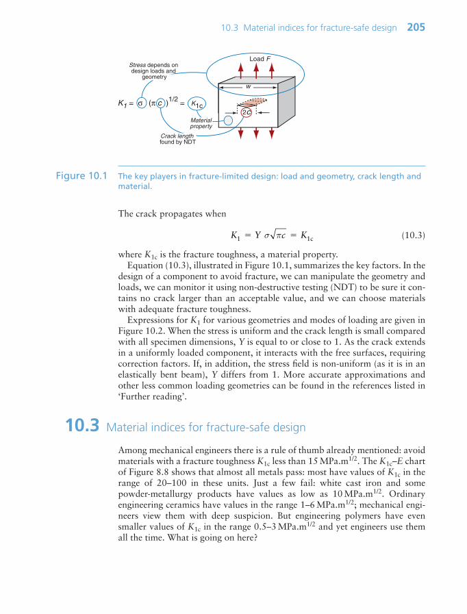
10.3 Material indices for fracture-safe design 205
The crack propagates when
(10.3)
where K1c is the fracture toughness, a material property.Equation (10.3), illustrated in Figure 10.1, summarizes the key factors. In the
design of a component to avoid fracture, we can manipulate the geometry andloads, we can monitor it using non-destructive testing (NDT) to be sure it con-tains no crack larger than an acceptable value, and we can choose materialswith adequate fracture toughness.
Expressions for K1 for various geometries and modes of loading are given inFigure 10.2. When the stress is uniform and the crack length is small comparedwith all specimen dimensions, Y is equal to or close to 1. As the crack extendsin a uniformly loaded component, it interacts with the free surfaces, requiringcorrection factors. If, in addition, the stress field is non-uniform (as it is in anelastically bent beam), Y differs from 1. More accurate approximations andother less common loading geometries can be found in the references listed in‘Further reading’.
10.3 Material indices for fracture-safe design
Among mechanical engineers there is a rule of thumb already mentioned: avoidmaterials with a fracture toughness K1c less than 15 MPa.m1/2. The K1c–E chartof Figure 8.8 shows that almost all metals pass: most have values of K1c in therange of 20–100 in these units. Just a few fail: white cast iron and some powder-metallurgy products have values as low as 10 MPa.m1/2. Ordinaryengineering ceramics have values in the range 1–6 MPa.m1/2; mechanical engi-neers view them with deep suspicion. But engineering polymers have evensmaller values of K1c in the range 0.5–3 MPa.m1/2 and yet engineers use themall the time. What is going on here?
K Y c K1 1c σ π
K1 = σ (π c )1/2 = K1c 2c
Load F
w
Materialproperty
Stress depends on design loads and
geometry
Crack length found by NDT
Figure 10.1 The key players in fracture-limited design: load and geometry, crack length andmaterial.
Ch10-H8391 1/17/07 11:39 AM Page 205

In a load-limited design—the structural member of a bridge or the wing-sparof an aircraft, for instance (Figure 10.3 (a, b))—the part will fail in a brittle wayif the stress exceeds that given by equation (10.3). To maximize the load wewant materials with highest values of
M1 K1c (10.4)
206 Chapter 10 Keeping it all together: fracture-limited design
Continued through crackK1 σπc (c w)
Single edge notchK1 1.1σπc (c w)
Through crack with pressure pK1 pπc (c w)
Cracked beam with central load F; b thickness
K1 3 FL——bw2
πc (c w)
Contained, penny-shaped crackK1 0.7σπc (c w)
σ
σ
σ
2w
2cr
2w
c
p
2w
2c
p
F
c
Lt
F/2F/2
2c
2w
σ
Figure 10.2 Stress intensities K1 associated with short cracks.
Ch10-H8391 1/17/07 11:39 AM Page 206

But not all designs are load limited; some are energy limited, others aredeflection limited. Then the criterion for selection changes. Consider, then, theother two scenarios sketched in Figure 10.3.
Energy-limited designNot all design is load limited. Springs and containment systems for turbinesand flywheels (to catch the bits if they disintegrate) are energy limited. Take thespring (Figure 10.3(c)) as an example. The elastic energy Ue stored in it is theintegral over the volume of the energy per unit volume, Ue, where
The stress is limited by the fracture stress of equation (10.3) so that—if ‘failure’means ‘fracture’—the maximum energy per unit volume that the spring canstore is
For a given initial flaw size c, the energy is maximized by choosing materialswith large values of
(10.5)
where Gc is the toughness, defined in Chapter 8.
MK
EG2
2 1c
c≈
UY
c
K
Eemax 1c
2 2
2π
⎛
⎝⎜⎜⎜⎜
⎞
⎠⎟⎟⎟⎟⎟
UEe
12
12
2σε
σ
10.3 Material indices for fracture-safe design 207
F(a)
(b)
(c) (d)
FF
Figure 10.3 (a, b) Load-limited design. (c) Energy-limited design. (d) Displacement-limiteddesign. Each must perform its function without fracturing.
Ch10-H8391 1/17/07 11:39 AM Page 207

Displacement-limited designThere is a third scenario: that of displacement-limited design (Figure 10.3(d)).Snap-on bottle tops, elastic hinges and couplings are displacement limited: theymust allow sufficient elastic displacement to permit the snap-action or flexurewithout failure, requiring a large failure strain εf. The strain is related to thestress by Hooke’s law, ε σ/E, and the stress is limited by the fracture equation(10.3). Thus, the failure strain is
The best materials for displacement-limited design are those with large values of
(10.6)
Plotting indices on chartsFigure 10.4 shows the K1c–E chart again. It allows materials to be compared by values of fracture toughness, M1, by toughness, M2, and by values of thedeflection-limited index, M3. As the engineer’s rule of thumb demands, almostall metals have values of K1c that lie above the 15 MPa.m1/2 acceptance level for load-limited design, shown as a horizontal selection line in the figure. Poly-mers and ceramics do not.
MK
E3 1c
επ
fmax
1cC
c
K
E
208 Chapter 10 Keeping it all together: fracture-limited design
100
10
1
0.1
0.01
Young's modulus, E (GPa)
Frac
ture
toug
hnes
s, K
1c (
MP
a.m
1/2 )
0.001 0.01 0.1 1 10 100 1000
0.01
0.1
1
10
100
1000
Foams
Polymers and elastomers
Metals
Technicalceramics
Composites Natural materials
Lead alloys
W alloys
SteelsTi alloys
Mg alloys
CFRPGFRP
Al alloys
Rigid polymer foams
Flexible polymer foams
Ni alloysCu alloys
Zinc alloys
PS
PTFE
PC
Cork
Wood
Butyl rubber
Silicone elastomers
Concrete
Al2O3
SiCSi3N4
Fracture toughness–Modulus
B4C
PP
EVAPolyurethane
Leather
Non-technical ceramics
Cast irons
WC
Soda glassSilica glass
Silicon
Stone
Brick
ABS
Epoxies
Ionomers
MFA, 07
Toughness Gc = (K1c)2/E kJ/m2
GFR
Cork
Cast Ca
WoodLeather0.1
merer
i alloys
K1c
K1c /E
K1c/E2
PA
Figure 10.4 The K1c–E chart showing the three indices M1, M2 and M3.
Ch10-H8391 1/17/07 11:39 AM Page 208
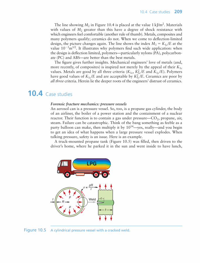
The line showing M2 in Figure 10.4 is placed at the value 1 kJ/m2. Materialswith values of M2 greater than this have a degree of shock resistance withwhich engineers feel comfortable (another rule of thumb). Metals, composites andmany polymers qualify; ceramics do not. When we come to deflection-limiteddesign, the picture changes again. The line shows the index M3 K1c/E at thevalue 103m1/2. It illustrates why polymers find such wide application: whenthe design is deflection limited, polymers—particularly nylons (PA), polycarbon-ate (PC) and ABS—are better than the best metals.
The figure gives further insights. Mechanical engineers’ love of metals (and,more recently, of composites) is inspired not merely by the appeal of their K1cvalues. Metals are good by all three criteria (K1c, K2
1c /E and K1c /E). Polymershave good values of K1c/E and are acceptable by K2
1c /E. Ceramics are poor byall three criteria. Herein lie the deeper roots of the engineers’ distrust of ceramics.
10.4 Case studies
Forensic fracture mechanics: pressure vesselsAn aerosol can is a pressure vessel. So, too, is a propane gas cylinder, the bodyof an airliner, the boiler of a power station and the containment of a nuclearreactor. Their function is to contain a gas under pressure—CO2, propane, air,steam. Failure can be catastrophic. Think of the bang something as feeble as aparty balloon can make, then multiply it by 1014—yes, really—and you beginto get an idea of what happens when a large pressure vessel explodes. Whentalking pressure, safety is an issue. Here is an example.
A truck-mounted propane tank (Figure 10.5) was filled, then driven to thedriver’s home, where he parked it in the sun and went inside to have lunch,
10.4 Case studies 209
Rt
p
p
c
t
pRt
σ =
Weld
Figure 10.5 A cylindrical pressure vessel with a cracked weld.
Ch10-H8391 1/17/07 11:39 AM Page 209

leaving the engine running. As he was drinking his coffee the tank exploded,causing considerable property damage and one death. The tank was made ofrolled AISI 1030 steel plate, closed by a longitudinal weld and two domesjoined to the rolled plate by girth welds. The failure occurred through the lon-gitudinal weld, causing the tank to burst (see cover picture). Subsequent exam-ination showed that the weld had contained a surface crack of depth 10 mmthat had been there for a long time, as indicated by discoloration and by stria-tions showing that it was growing slowly by fatigue each time the tank wasemptied and refilled. At first sight it appears that the crack was the direct causeof the failure.
That’s where fracture mechanics comes in. Measurements on a section of thetank wall gave a fracture toughness of 45 MPa.m1/2. The dimensions of the tankare listed in Table 10.1. It was designed for a working pressure of 1.4 MPa, lim-ited at 1.5 MPa by a pressure release valve.
The tensile stress in the wall of a thin-walled cylindrical pressure vessel ofradius R and wall thickness t containing a pressure p (Figure 10.5) was given inChapter 4. With the values listed above the stress in the tank wall is
(10.7)
A plate with a fracture toughness 45 MPa.m1/2 containing a surface crack ofdepth 10 mm will fail at the stress
This is 2.5 times higher than the stress in the tank wall. The pressure needed togenerate this stress is 3.8 MPa—far higher than the safety limit of 1.5 MPa.
At first it appears that the calculations cannot be correct since the tank hada relief valve set at the working pressure, but the discrepancy prompted theinvestigators to look further. An inspection of the relief valve showed rust andcorrosion, rendering it inoperative. Further tests confirmed that heat from thesun and from the exhaust system of the truck raised the temperature of thetank, vaporizing the liquefied gas and driving the pressure past the value of3.8 MPa needed to make the crack propagate. The direct cause of the failurewas the jammed pressure release valve. The crack would not have propagatedat the normal operating pressure.
σπ
K
c1c MPa
1 1231
.
σ pRt
90 MPa
210 Chapter 10 Keeping it all together: fracture-limited design
Maximum design pressure, p 1.5 MPaWall thickness, t 14 mm (thicker at weld)Outer diameter, 2R 1680 mmLength, L 3710 mm
Table 10.1 Tank dimensions
Ch10-H8391 1/17/07 11:39 AM Page 210
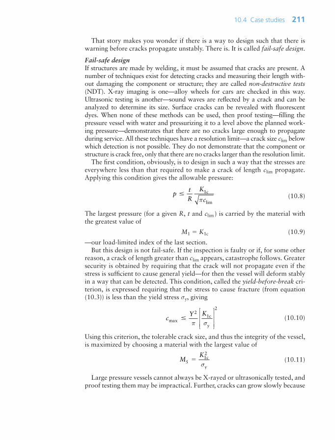
That story makes you wonder if there is a way to design such that there iswarning before cracks propagate unstably. There is. It is called fail-safe design.
Fail-safe designIf structures are made by welding, it must be assumed that cracks are present. Anumber of techniques exist for detecting cracks and measuring their length with-out damaging the component or structure; they are called non-destructive tests(NDT). X-ray imaging is one—alloy wheels for cars are checked in this way.Ultrasonic testing is another—sound waves are reflected by a crack and can beanalyzed to determine its size. Surface cracks can be revealed with fluorescentdyes. When none of these methods can be used, then proof testing—filling thepressure vessel with water and pressurizing it to a level above the planned work-ing pressure—demonstrates that there are no cracks large enough to propagateduring service. All these techniques have a resolution limit—a crack size clim belowwhich detection is not possible. They do not demonstrate that the component orstructure is crack free, only that there are no cracks larger than the resolution limit.
The first condition, obviously, is to design in such a way that the stresses areeverywhere less than that required to make a crack of length clim propagate.Applying this condition gives the allowable pressure:
(10.8)
The largest pressure (for a given R, t and clim ) is carried by the material withthe greatest value of
M1 K1c (10.9)
—our load-limited index of the last section.But this design is not fail-safe. If the inspection is faulty or if, for some other
reason, a crack of length greater than clim appears, catastrophe follows. Greatersecurity is obtained by requiring that the crack will not propagate even if thestress is sufficient to cause general yield—for then the vessel will deform stablyin a way that can be detected. This condition, called the yield-before-break cri-terion, is expressed requiring that the stress to cause fracture (from equation(10.3)) is less than the yield stress σy, giving
(10.10)
Using this criterion, the tolerable crack size, and thus the integrity of the vessel,is maximized by choosing a material with the largest value of
(10.11)
Large pressure vessels cannot always be X-rayed or ultrasonically tested, andproof testing them may be impractical. Further, cracks can grow slowly because
MK
5 1c2
yσ
cY K
max1c
y
2
2
π σ
⎡
⎣
⎢⎢⎢
⎤
⎦
⎥⎥⎥
ptR
K
c 1c
π lim
10.4 Case studies 211
Ch10-H8391 1/17/07 11:39 AM Page 211

of corrosion or cyclic loading, so that a single examination at the beginning ofservice life is not sufficient. Then safety can be ensured by arranging that acrack just large enough to penetrate both the inner and the outer surface of thevessel is still stable, because the leak caused by the crack can be detected. Thiscondition, called the leak-before-break criterion, is achieved by setting 2c tin equation (10.3), giving
(10.12)
The wall thickness t of the pressure vessel must also contain the pressure p with-out yielding. From equation (10.7), this means that
Substituting this into the previous equation (with σ σf) gives
The pressure is carried most safely by the material with the greatest value of
(10.13)
Both M4 and M5 could be made large by making the yield strength of thewall, σy, very small: lead, for instance, has high values of both, but you wouldnot choose it for a pressure vessel. That is because the vessel wall must also bethin, both for economy of material and to keep it light. The thickness of thewall, from equation (10.7), is inversely proportional to the yield strength, σy.Thus, we wish also to maximize
M6 σy (10.14)
narrowing further the choice of material.The way to explore these criteria is to use the K1c – σy chart introduced in
Chapter 8. The indices M1, M4, M5 and M6 can be plotted onto it as lines ofslope 0, 1, 1/2 and as lines that are vertical. Take ‘leak-before-break’ as anexample. A diagonal line corresponding to a constant value of M5 K2
1c /σylinks materials with equal performance; those above the line are better. The lineshown in the figure excludes everything but the toughest steels, copper, nickeland titanium alloys. A second selection line for M6 at σy 200 MPa narrows theselection further. Exercises at the end of this chapter develop further examples ofthe use of the others.
Boiler failures used to be commonplace—there are even songs about it. Nowthey are rare, though when safety margins are pared to a minimum (rockets) or
MK
5 1c2
yσ
pYR
K
4 2 2
π σ1c
y
⎛
⎝
⎜⎜⎜⎜⎜
⎞
⎠
⎟⎟⎟⎟⎟⎟
tpR
2σy
σπ
Y K
t1c
/2
212 Chapter 10 Keeping it all together: fracture-limited design
Ch10-H8391 1/17/07 11:39 AM Page 212

maintenance is neglected (the propane tank) pressure vessels still occasionally fail.This (relative) success is one of the major contributions of fracture mechanicsto engineering practice.
Materials to resist fatigue: con-rods for high-performance enginesThe engine of a family car is designed to tolerate speeds up to about6000 rpm—100 revolutions per second. That of a Formula 1 racing car revs toabout three times that. Comparing an F1 engine to that of a family car is likecomparing a Rolex watch to an alarm clock, and their cost reflects this: about$200 000 per engine. Performance, here, is everything.
The connecting rods of a high-performance engine are critical components:if one fails the engine self-destructs. Yet to minimize inertial forces and bearingloads, each must weigh as little as possible. This implies the use of light, strongmaterials, stressed near their limits. When minimizing cost not maximizing per-formance is the objective, con-rods are made from cast iron. But here we wantperformance. What, then, are the best materials for such con-rods?
An F1 engine is not designed to last long—about 30 hours—but 30 hours ataround 15 000 rpm means about 3 106 cycles of loading and that meanshigh-cycle fatigue. For simplicity, assume that the shaft has a uniform section
10.4 Case studies 213
Yield strength or elastic limit, σy (MPa)
Fra
ctur
e to
ughn
ess,
K1c
(M
Pa.
m1/
2 )
0.1 1 10 100 1000
0.01
0.1
1
10
100
1000
0.01
Non-technical ceramics
Foams
Polymers and elastomers
Metals
Technicalceramics
CompositesLead alloys
W alloys
Stainless steels
Ti alloys
Mg alloys
CFRP
GFRP
Al alloys
Rigid polymer foams
Flexible polymer foams
Ni alloys
Cu alloys
Zinc alloys
PMMA
Cork
Wood
Butyl rubber
Silicone elastomers
Concrete
Al2O3
SiCSi3N4
Fracture toughness–Strength
B4C
Neoprene
Isoprene
Leather
Castirons
WC
Soda glass
Silica glassSilicon
Stone
Brick
ABS
Epoxies
Ionomers
Low alloy steels
Carbon steels
Polyurethane
PAPC
PEPTFE
PS
PP
Phenolic
MFA, 07
Leather
B
IonomersRP
A
ss
c
σy
K1c /σy2
Figure 10.6 Selecting the best materials for leak-before-break design. The additionalrequirement of high yield strength is also shown. The best choices are thematerials in the small area at the top right.
Ch10-H8391 1/17/07 11:39 AM Page 213

of area A and length L (Figure 10.7) and that it carries a cyclic load F. Itsmass is
m AL ρ (10.15)
where ρ is the density. The fatigue constraint requires that
where σe is the endurance limit of the material of which the con-rod is made.Using this to eliminate A in equation (10.15) gives an equation for the mass:
containing the material index
(10.16)
Materials with high values of this index are identified by creating a chart withσe and ρ as axes, applying an additional, standard, constraint that the fracturetoughness exceeds 15 MPa.m1/2 (Figure 10.8). Materials near the top-left cornerare attractive candidates: high-strength magnesium, aluminum and ultra-high-strength steels; best of all are titanium alloys and CFRP. This last material has beenidentified by others as attractive in this application. To go further we need S–Ncurves for the most attractive candidates. Figure 10.9 shows such a curve for themost widely used of titanium alloys: the alloy Ti–6Al–4V. The safe stress ampli-tude at R 1 for a design life of 2.5 106 cycles can be read off: it is 620 MPa.
M σρe
m F ρσe
⎛
⎝⎜⎜⎜⎜
⎞
⎠⎟⎟⎟⎟⎟
FA
σe
214 Chapter 10 Keeping it all together: fracture-limited design
Cross-sectionarea A
L
Figure 10.7 A connecting rod.
Ch10-H8391 1/17/07 11:39 AM Page 214
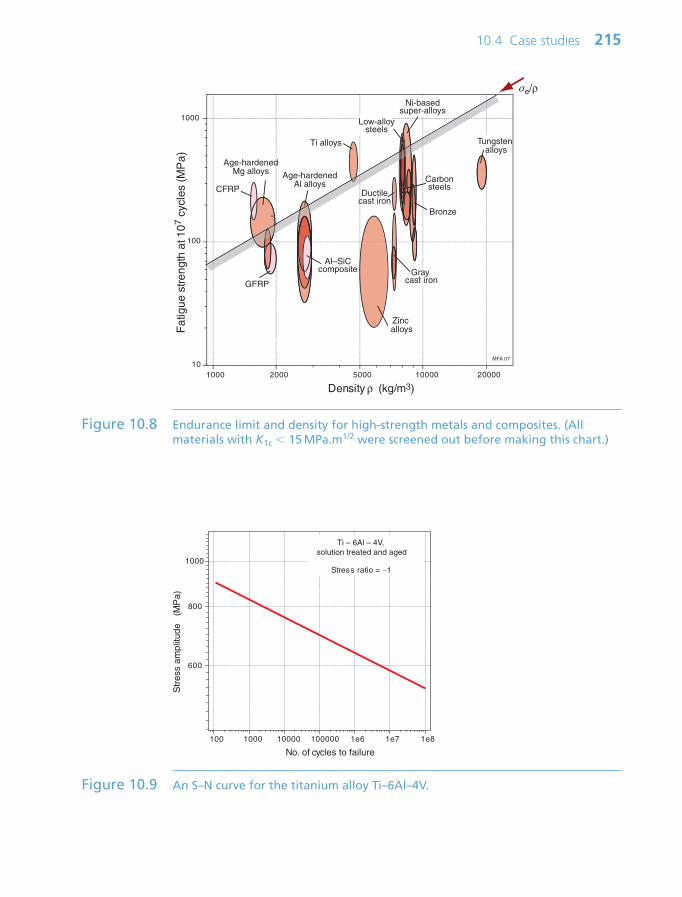
10.4 Case studies 215
No. of cycles to failure
100 1000 10000 100000 1e6 1e7 1e8
600
800
1000
Str
ess
ampl
itude
(M
Pa)
Ti – 6Al – 4V, solution treated and aged
Stress ratio = −1
Figure 10.9 An S–N curve for the titanium alloy Ti–6Al–4V.
Density ρ (kg/m3)1000 2000 5000 10000 20000
Fat
igue
stre
ngth
at 1
07 c
ycle
s (M
Pa)
10
100
1000
Age-hardenedAl alloys
Zinc alloys
CFRP
GFRP
Age-hardenedMg alloys
Ti alloys Tungsten alloys
Low-alloysteels
Ni-basedsuper-alloys
Gray cast iron
Bronze
Ductilecast iron
Carbonsteels
Al–SiCcomposite
σe/ρ
MFA 07
Figure 10.8 Endurance limit and density for high-strength metals and composites. (Allmaterials with K1c 15 MPa.m1/2 were screened out before making this chart.)
Ch10-H8391 1/17/07 11:39 AM Page 215
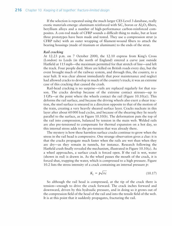
If the selection is repeated using the much larger CES Level 3 database, reallyexotic materials emerge: aluminum reinforced with SiC, boron or Al2O3 fibers,beryllium alloys and a number of high-performance carbon-reinforced com-posites. A con-rod made of CFRP sounds a difficult thing to make, but at leastthree prototypes have been made and tested. They use a compression strut (aCFRP tube) with an outer wrapping of filament-wound fibers to attach thebearing housings (made of titanium or aluminum) to the ends of the strut.
Rail crackingAt 12.23 p.m. on 7 October 2000, the 12.10 express from King’s Cross(London) to Leeds (in the north of England) entered a curve just outsideHatfield at 115 mph—the maximum permitted for that stretch of line—and leftthe track. Four people died. More are killed on British roads every day, but theevent brought much of the railway system, and through this, the country, to anear halt. It was clear almost immediately that poor maintenance and neglecthad allowed cracks to develop in much of the country’s track; it was an extremecase of this cracking that caused the crash.
Rail-head cracking is no surprise—rails are replaced regularly for that rea-son. The cracks develop because of the extreme contact stresses—up to1 GPa—at the point where the wheels contact the rail (Figure 10.10(a)). Thisdeforms the rail surface, and because the driving wheels also exert a shear trac-tion, the steel surface is smeared in a direction opposite to that of the motion ofthe train, creating a very heavily sheared surface layer. Cracks nucleate in thislayer after about 60 000 load cycles, and because of the shearing they lie nearlyparallel to the surface, as in Figure 10.10(b). The deformation puts the top ofthe rail into compression, balanced by tension in the main web. Welded railsare also pre-tensioned to compensate for thermal expansion on a hot day, sothis internal stress adds to the pre-tension that was already there.
The mystery is how these harmless surface cracks continue to grow when thestress in the rail head is compressive. One strange observation gives a clue: it isthat the cracks propagate much faster when the rails are wet than when theyare dry—as they remain in tunnels, for instance. Research following theHatfield crash finally revealed the mechanism, illustrated in Figure 10.10(c). Asa wheel approaches, a surface crack is forced open. If the rail is wet, water(shown in red) is drawn in. As the wheel passes the mouth of the crack, it isforced shut, trapping the water, which is compressed to a high pressure. Figure10.2 lists the stress intensity of a crack containing an internal pressure p:
(10.17)
So although the rail head is compressed, at the tip of the crack there is tension—enough to drive the crack forward. The crack inches forward anddownward, driven by this hydraulic pressure, and in doing so it grows out ofthe compression field of the head of the rail and into the tensile field of the web.It is at this point that it suddenly propagates, fracturing the rail.
K p cl π
216 Chapter 10 Keeping it all together: fracture-limited design
Ch10-H8391 1/17/07 11:39 AM Page 216

The answer—looking at equation (10.17)—is to make sure the surface cracksdo not get too long; Kl for a short pressurized crack is small, for a long one itis large. Proper rail maintenance involves regularly grinding the top surface ofthe track to remove the cracks, and when this has caused significant loss of sec-tion, replacing the rails altogether.
Fatigue crack growth: living with cracksThe crack in the LPG tank of the earlier case study showed evidence of stria-tions: ripples marking the successive positions of the crack front as it slowlyadvanced, driven by the cyclic pressurizing of the tank. The cause of the explo-sion was over-pressure caused by poor maintenance, but suppose maintenancehad been good and no over-pressure had occurred. How long would it havelasted before fatigue grew the crack to an unstable size? We calculate this size,c*, by inverting equation (10.3):
(10.18)cK
Y* lc
2
2 2πσ
10.4 Case studies 217
Railhead
Wheel
Contact zone
Web
Compressedsurface layer
Main body of rail in tension
Direction of traffic
Surfacecracks
Crackpenetrating rail
Direction of traffic
Crack opens, sucks in water
Crack closes, compresses water
K1
(a)
(b)
(c)
Figure 10.10 Rail cracking. (a) The rolling contact. (b) The surface cracks, one of which haspenetrated the part of the rail that is in tension. (c) The mechanism by whichthe crack advances.
Ch10-H8391 1/17/07 11:39 AM Page 217

With Klc 45 MPa.m1/2, σ 90 MPa and Y 1, the answer is c* 80 mm.How long will it take to grow that big? A week? A month? Twenty years?
This sort of question arises in assessing the safety of large plant that (becauseof welds) must be assumed to contain cracks: the casing of steam turbines, chem-ical engineering equipment, boilers and pipe-work. The cost of replacement of alarge turbine casing is considerable and there is associated down-time. It does notmake sense to take it out of service if, despite the crack, it is perfectly safe.
Fatigue crack growth was described in Chapter 9. Its rate is described by theequation
(10.19)
in which the cyclic stress intensity range, ∆K, is
Inserting this into equation (10.19) gives
(10.20)
The residual life, NR, is found by integrating this between c ci (the initialcrack length) and c c*, the value at which fast fracture will occur:
(10.21)
We shall suppose the steel of which the tank is made has a crack-growth expo-nent m 4 and a value of A 2.5 106 when ∆σ is in MPa. Taking the ini-tial crack length as 10 mm, the integral gives
Assuming that the tank is pressurized once per day, it will last forever.The calculation illustrates how life-limited fatigue crack growth is calcu-
lated. It ignored the fact that the tank wall was only 12 mm thick. The crackwill penetrate the wall, releasing propane and revealing its presence, longbefore it is 80 mm long. In this sense, the tank is fail-safe provided the stressamplitude does not exceed 1.5 MPa.
Designing for fractureManufacturers who distribute their products packaged in toughened envelopes,sheathed in plastic, or contained in aluminum or steel cans, need to design thecontainment so that the purchaser can get at the contents. As you will know,not all do—even getting the wrapper off a newly purchased CD is a pain. And
NA c cR
i
cycles 1 1 1
7 104
6
∆σ *
⎛
⎝⎜⎜⎜⎜
⎞
⎠⎟⎟⎟⎟⎟
N NA
cc
N
m mc
c
R /
*R d
d( )i
0 2
1∫ ∫∆σ π
dd
( ) /cN
A cm m ∆σ π 2
∆ ∆K K K c max min σ π
dd
cN
A Km ∆
218 Chapter 10 Keeping it all together: fracture-limited design
Ch10-H8391 1/17/07 11:39 AM Page 218

there is a more serious dimension. Producers of foods, drugs, chemicals, evenwashing powder, now package their products in ‘break to access’ packaging sothat the purchaser knows that it has not been tampered with. How do youarrange protection and yet enable fracture? One part of the answer is to choosethe right material; the other is to provide stress concentrations to focus stresson the break-lines or to use adhesives that have high shear strength but low peelresistance.
Start with material: materials with low ductility, in thin sheets, tear easily. If‘opening’ means pulling in such a way as to tear (as it often does), then the firststep is a to choose a material with adequate stiffness, strength and durability,but low ductility. The lids of top-opening drinks cans are made of a differentalloy than the can itself for exactly this reason.
Next, stress concentration. This means reducing the section by grooving orserrating the package locally along the line where tearing is wanted. Toiletpaper, as we all know, hardly ever tears along the perforations, but it was theright idea. The sardine can on the cover of this chapter is made of low-ductilityaluminum alloy with a groove with a sharp radius of curvature along the tearline to provide a stress concentration factor (Chapter 7) of
(10.22)
where c is the groove depth and ρ its root radius and the factor 1⁄2 appearsbecause the loading is shear rather than tension. A 0.2 mm groove with rootradius of 0.02 mm gives a local stress that is 2.5 times higher than that else-where, localizing the tearing at the groove.
The peel-strip of a CD wrapper is not a groove; it is an additional thickerstrip. How does this apparent reinforcement make it easier to tear open thepackage? Figure 7.7 provides the answer: it is because any sudden change of sec-tion concentrates stress. If the strip thickness is c and the radius where it joinsthe wrapping is ρ, the stress concentration is still given by equation (10.22).
The alternative to tearing is adhesive peeling. Figure 10.11 shows an adhe-sive joint before and during peeling. The adhesive has shear strength σs* andtoughness Gc*. Adhesively bonded packaging must accept in-plane tension,since to protect the content it must support the mass of its contents and hand-ling loads. The in-plane pull force Ft that the joint can carry without failing is
Ft σs* A σs* w L
where A wL is the area of the bonded surface. To open it, a peel force Fp isapplied. The lower part of Figure 10.11 shows how Fp does work when the jointis peeled back by a distance δx, creating new surface of area w δx. This requiresand energy Gc* w δx (since Gc*, the toughness, is the energy to create unit areaof new surface). The work done by Fp must provide this energy, giving
Kc
sc ≈⎛
⎝
⎜⎜⎜⎜⎜
⎞
⎠
⎟⎟⎟⎟⎟1
12
ρ
10.4 Case studies 219
Ch10-H8391 1/17/07 11:39 AM Page 219

Fp δx Gc* w δx
Thus, Fp w Gc* The ratio of the peel force to the tensile force is
Adhesive joints are designed to have a particular value for this ratio. The choiceof adhesive sets the values of Gc* and σs*, allowing the length L to be chosen togive tensile strength with ease of peeling.
10.5 Summary and conclusions
Elastic deformation is recoverable. Plastic deformation is gradual anddetectable before really bad things happen. Failure by fast fracture is none ofthese. It has been the cause of many great engineering disasters: collapsedbridges, burst boilers, rail accidents, aircraft crashes.
A component will fail by fast fracture if the stress intensity K1 at any crack-like defect it contains exceeds the fracture toughness K1c of the material ofwhich it is made. The understanding of fast fracture and the development ofdesign methods to deal with it are relatively new—before 1950 little wasknown. Both are now on a solid basis. This chapter introduced them, describ-ing the ways in which K1 is calculated, how K1c is measured and the variousscenarios in which it is relevant. It ended with examples of their application.
Much the same is true of failure by fatigue. A seemingly healthy component,one that has served its purpose well, fails without warning because an initiallysmall and harmless crack has grown until it reached the size at which fast fracture
F
F
G
Lp
t
c
s
*
σ∗
220 Chapter 10 Keeping it all together: fracture-limited design
Fp
Ft FtL
w
δx
δx
Adhesive
Figure 10.11 Peeling of an adhesive bond.
Ch10-H8391 1/17/07 11:39 AM Page 220

takes over. Small components may, initially, be crack free, but cyclic loadingcan lead to crack nucleation and subsequent growth; design is then based onthe S–N curve of the material. Larger structures, particularly those that arewelded, cannot be assumed to be crack free; then the life is estimated from thepredicted rate of crack growth, integrating it to find the number of cycles togrow the crack to a dangerous size.
Fracture, however, is not always bad. Enabling fracture allows you to get atthe contents of shrink-wrapped packages, access food and drugs in tamper-proof containers and at drinks in pop-top cans. Here the trick is to design-instress concentrations that create locally high stresses along the desired fracturepath, and to choose a material with adequate strength but low ductility.
10.6 Further reading
Broek, D. (1981) Elementary Engineering Fracture Mechanics, 3rd edition, MartinusNijhoff, Boston, USA. ISBN 90-247-2580-1. (A standard, well-documented, intro-duction to the intricacies of fracture mechanics.)
Ewalds, H.L. and Wanhill, R.J.H. (1984) Fracture Mechanics, Edward Arnold, London,UK. ISBN 0-7131-3515-8. (An introduction to fracture mechanics and testing forboth static and cyclic loading.)
Hertzberg, R.W. (1989) Deformation and Fracture of Engineering Materials, 3rd edi-tion, Wiley, New York, USA. ISBN 0-471-63589-8. (A readable and detailed coverageof deformation, fracture and fatigue.)
Hudson, C.M. and Rich, T.P. (eds) (1986) Case Histories Involving Fatigue andFracture Mechanics, ASTM STP 918, American Society for Testing and Materials,USA. ISBN 0-8031-0485-5. (A compilation of case studies of fatigue failures, many ofthem disastrous, analyzing what went wrong.)
Suresh, S. (1998) Fatigue of Materials, 2nd edition, Cambridge University Press,Cambridge, UK. ISBN 0-521-57847-7. (The place to start for an authoritative introduction to the materials science of fatigue in both ductile and brittle materials,with case studies.)
Tada, H., Paris, G. and Irwin, G.R. (2000) The Stress Analysis of Cracks Handbook,3rd edition. ISBN 1-86058-304-0. (A comprehensive catalog of stress intensity fac-tors for a great range of geometries and modes of loading.)
10.7 Exercises
10.7 Exercises 221
Exercise E10.1 Supersonic wind tunnels store air under high pressure in cylindrical pressurevessels—the pressure, when released, produces hypersonic rates of flow. Thepressure vessels are routinely proof tested to ensure that they are safe. If sucha cylinder, of diameter 400 mm and wall thickness 20 mm, made of a steel
Ch10-H8391 1/17/07 11:39 AM Page 221

222 Chapter 10 Keeping it all together: fracture-limited design
with a fracture toughness of 42 MPa.m1/2, survives a proof test to 40 MPa(400 atmospheres), what is the length of the largest crack it might contain?
Exercise E10.2 You are asked to select a polymer to make a flexible coupling. The polymermust have a modulus greater than 2 GPa. The objective is to maximize theavailable flexure without fracture. Use the chart of Figure 10.4 to identifytwo good choices to meet these requirements. Are there any metals that areas good?
Exercise E10.3 Crash barriers like car fenders must absorb energy without total fracture.The most effective are those that deform plastically, absorbing energy in plas-tic work, but they are not reusable. Fenders that remain elastic spring backafter impact. For practical reasons the material must have a modulus greaterthan 10 GPa. Use the chart of Figure 10.4 to find non-metallic materials forelastic fenders, assuming that the overriding consideration is that the dis-placement before fracture is as great as possible (the constraint on modulusensures that it absorbs enough energy).
Exercise E10.4 Materials with high toughness Gc generally have high modulus. Sometimes,however, the need is for high toughness with low modulus, so that the com-ponent has some flexibility. Use the chart of Figure 10.4 to find the material(from among those on the chart) that has a modulus less than 0.5 GPa andthe highest toughness Gc. List applications of this material that you can thinkof that exploit this combination of properties.
Exercise E10.5 If you want to support a precision optical system (laser metrology equip-ment, for instance) on a stable platform, you put it on a granite slab sup-ported on end plinths to bring it to working height. (Granite can be groundto a flat surface and is thermally very stable and hard wearing.) The granitechosen for one such table has a fracture toughness of 0.9 MPa.m1/2 and isknown, from NDT procedures, to contain internal cracks up to 5 mm inlength. If the table is 2 m long and 1 m deep, simply supported at its ends andmust carry a uniformly distributed load of 2000 N on its upper surface (as inFigure 7.2 of the text), what is the minimum thickness the slab must have?Include the self-weight of the slab in the analysis. Assume that at least one ofthe cracks will lie in the part of the beam that carries the highest tensilestress—that is, at the lower surface (the density of granite is 2700 kg/m3).
Exercise E10.6 The figure below shows, in (a), a cylindrical tie-rod with diameter 20 mm.The plan is to use it to carry a cyclic load with a stress range 200 kN. Thefigure also shows the S–N curve of the material of which it is to be made.Will it survive without failure for at least 105 cycles?
Ch10-H8391 1/17/07 11:39 AM Page 222

Exercise E10.7 The component of the previous exercise was made and tested. It failed in lessthan 105 cycles. A post-mortem revealed that it had fractured at the root of athreaded end, shown in (b) in the figure. The threads have a depth of 1.5 mmand a root radius of 0.2 mm. Given this additional information, how manycycles would you expect it to survive?
Exercise E10.8 An adhesive has a toughness Gc 100 J/m2 and a shear strengthσs 0.1 MPa. What must the dimensions of the bonded area of a lap-jointbe if it is to carry an in-plane tensile Ft of 100 N but allow peeling at a forceFp of 5 N?
Exercise E10.9 The figure on next page shows a component to be made from the high-strength aerospace alloy Ti–6Al–4V. It will be loaded cyclically at a nominalstress range of 210 MPa. How long will it last?
10.7 Exercises 223
20 mm
20 mm
Thread depth 1.5 mmRoot radius 0.2 mm
(a) (b)
Cyclic loading ±600 N
Number of cycles to failure, Nf
400
500
600
700
800
900
1000
1100
1200
1300
1400
1500
103 104 105 106 107 108102
Str
ess
ampl
itude
, σa
(MP
a)
4340 Low-alloy steel,quenched and tempered 425°C Stress ratio R = −1
Ch10-H8391 1/17/07 11:39 AM Page 223

224 Chapter 10 Keeping it all together: fracture-limited design
10.8 Exploring design with CES (use Level 2, Materials, for allselections)
Exercise E10.10 Use the ‘Search’ facility in CES to find materials that are used for:
(a) Pressure vessels.(b) Connecting rods.(c) Rail track.
(Search using the singular—e.g. pressure vessel—since that will find the plural too.)
Exercise E10.11 You are asked, as in Exercise E10.2, to select a polymer to make a flexiblecoupling. The polymer must have a modulus E greater than 2 GPa. Theobjective is to maximize, the available flexure without fracture, and thatmeans materials with high K1c/E. Use a ‘Limit’ stage to impose the constrainton E, then use a ‘Graph’ stage to make a chart for K1c and E, put on anappropriate selection line and move it until only three materials remain inthe Results window. What are they? Rank them by price.
Exercise E10.12 You are asked to recommend materials that have yield strength above500 MPa and perform best in a design based on the leak-before-break crite-rion. Construct an appropriate limit stage and chart, put on the necessaryselection line and list the three materials you would recommend.
24 mm
16 mm
Radius3 mm
± 210 MPa
No. of cycles to failure100 1000 10000 100000 1e6 1e7 1e8
600
800
1000
Str
ess
ampl
itude
(M
Pa)
Ti – 6Al – 4V, solution treated and aged
Stress ratio = −1
Ch10-H8391 1/17/07 11:39 AM Page 224

10.8 Exploring design with CES 225
Exercise E10.13 Repeat the previous selection, applying instead a yield-before-break selec-tion criterion.
Exercise E10.14 A material is sought for a high-performance con-rod, requiring that theindex has a high value of the index σe/ρ, where σe is the endurance limit (thefatigue strength at 107 cycles). It must have enough toughness to toleratestress concentrations, requiring that K1c 15 MPa.m1/2. Make the appropri-ate selection stages and list the three materials that best meet the criteria.
Ch10-H8391 1/17/07 11:39 AM Page 225

This page intentionally left blank

Chapter 11Rub, slither and seize:
friction and wear
Chapter contents
11.1 Introduction and synopsis 22811.2 Tribological properties 22811.3 Charting friction and wear 22911.4 The physics of friction and wear 23111.5 Design and selection: materials to
manage friction and wear 23511.6 Summary and conclusions 24011.7 Further reading 24111.8 Exercises 24111.9 Exploring design with CES 243
A disc brake (image courtesy Paul Turnbull, SEMTA,Watford, UK. www.gcseinenginering)
Ch11-H8391.qxd 1/16/07 6:05 PM Page 227

228 Chapter 11 Rub, slither and seize: friction and wear
11.1 Introduction and synopsis
God, it is said, created materials, but their surfaces are the work of the devil.They are certainly the source of many problems. When surfaces touch andslide, there is friction; and where there is friction, there is wear. Tribologists—the collective noun for those who study friction and wear—are fond of citingthe enormous cost, through lost energy and worn equipment, for which thesetwo phenomena are responsible. It is certainly true that, if friction could beeliminated, the efficiency of engines, gearboxes, drive trains and the like wouldincrease enormously; and if wear could be eradicated, they would also lastmuch longer. But before accepting this negative image, one should rememberthat, without wear, pencils would not write on paper or chalk on blackboards;and without friction, one would slither off the slightest incline.
Tribological properties are not attributes of one material alone, but of onematerial sliding on another with—almost always—a third in between. Thenumber of combinations is far too great to allow choice in a simple, systematicway. The selection of materials for bearings, drives and sliding seals relies heav-ily on experience. This experience is captured in reference sources (for which,see ‘Further reading’); in the end it is these that must be consulted. But it doeshelp to have a feel for the magnitude of friction coefficients and wear rates, andan idea of how these relate to material class. This chapter provides it.
11.2 Tribological properties
When two surfaces are placed in contact under a normal load Fn and one ismade to slide over the other, a force Fs opposes the motion. This force Fs is pro-portional to Fn but does not depend on the area of the surface, facts discoveredby none other than Leonardo da Vinci1, then forgotten, then rediscovered 200years later by Amontons2, whose name they carry. The coefficient of friction µis defined as in Figure 11.1:
(11.1)
When surfaces slide, they wear. Material is lost from both surfaces, evenwhen one is much harder than the other. The wear rate, W, is conventionallydefined as
µ F
Fs
n
1 Leonardo da Vinci (1452–1519), Renaissance painter, architect, engineer, mathematician,philosopher and prolific inventor.
2 Guillaume Amontons (1663–1705), French scientific instrument maker and physicist, per-fector of the clepsydra or water clock—a device for measuring time by letting water flowfrom a container through a tiny hole.
Ch11-H8391.qxd 1/16/07 6:05 PM Page 228
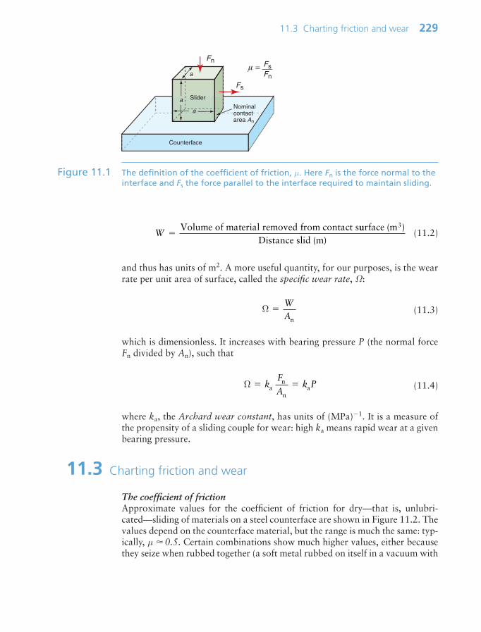
11.3 Charting friction and wear 229
(11.2)
and thus has units of m2. A more useful quantity, for our purposes, is the wearrate per unit area of surface, called the specific wear rate, Ω:
(11.3)
which is dimensionless. It increases with bearing pressure P (the normal forceFn divided by An), such that
(11.4)
where ka, the Archard wear constant, has units of (MPa)1. It is a measure ofthe propensity of a sliding couple for wear: high ka means rapid wear at a givenbearing pressure.
11.3 Charting friction and wear
The coefficient of frictionApproximate values for the coefficient of friction for dry—that is, unlubri-cated—sliding of materials on a steel counterface are shown in Figure 11.2. Thevalues depend on the counterface material, but the range is much the same: typ-ically, µ 0.5. Certain combinations show much higher values, either becausethey seize when rubbed together (a soft metal rubbed on itself in a vacuum with
Ω kF
Ak Pa
n
na
Ω WAn
W Volume of material removed from contact suurface m
Distance slid m( )
( )
3
Fs
µ = Fn
FsFn
Nominal contactarea An
Counterface
Slider
a
a
a
Figure 11.1 The definition of the coefficient of friction, µ. Here Fn is the force normal to theinterface and Fs the force parallel to the interface required to maintain sliding.
Ch11-H8391.qxd 1/16/07 6:05 PM Page 229

no lubrication, for instance) or because one surface has a sufficiently low mod-ulus that it conforms to the rough surface of the other (rubber on rough con-crete). At the other extreme are sliding combinations with exceptionally lowcoefficients of friction, such as PTFE, or bronze bearings loaded with graphite,sliding on polished steel. Here the coefficient of friction falls as low as 0.04,though this is still high compared with friction for lubricated surfaces, as notedat the bottom of the diagram.
The wear rate – hardness chartFigure 11.3 shows the Archard wear constant ka plotted against hardness, hereexpressed in MPa. (Hardness in MPa 10 Vickers hardness, HV.) The bear-ing pressure P is the quantity specified by the design. The ability of a surface toresist a static contact pressure is measured by its hardness, so the maximumbearing pressure Pmax is just the hardness H of the softer surface. Thus, thewear rate of a bearing surface can be written:
Two material properties appear in this equation: the wear constant ka and thehardness, H—they are the axes of the chart. The diagonal contours show theproduct
K ka H (11.5)
Ω k P kP
PHa a
max
⎛
⎝⎜⎜⎜⎜
⎞
⎠⎟⎟⎟⎟⎟
230 Chapter 11 Rub, slither and seize: friction and wear
Coe
ffici
ent o
f fric
tion
on d
ry s
teel
, µ
0.01
0.1
1
10
Lead alloys
Low carbon steels
Al alloys
Cu alloys
PA
PMMA
Wood
Butyl rubber
Cast irons
WC
Coefficient of friction
PTFE
Leather
MFA, 07
PP
PE
Soda glass
Natural rubber
Borosilicate glass
PS
µ for boundary lubrication = 0.01–0.1µ for full hydrodynamic lubrication = 0.001–0.01
Figure 11.2 The coefficient of friction µ of materials sliding on an unlubricated steel surface.
Ch11-H8391.qxd 1/16/07 6:05 PM Page 230

The best materials for bearings for a given bearing pressure P are those with thelowest value of ka—that is, those nearest the bottom of the diagram. On theother hand, an efficient bearing, in terms of size or weight, will be loaded to asafe fraction of its maximum bearing pressure—that is, to a constant value ofP/Pmax—and for these, materials with the lowest values of the product ka H arebest. Materials of a given class (metals, for instance) tend to lie along a down-ward sloping diagonal across the figure, reflecting the fact that low wear rate isassociated with high hardness.
11.4 The physics of friction and wear3
FrictionSurfaces, no matter how meticulously honed and polished, are never perfectlyflat. The roughness, defined in Chapter 18, depends on how the surface was
11.4 The physics of friction and wear 231
Hardness, H (MPa)
Wea
r rat
e co
nsta
nt ,
k a (1
/(MP
a))
10 100 1000 10 000 100 00010−11
10−10
10−9
10−8
10−7
10−6
10−5
10−4
10−6
10−7
10−5
10−4
10−3Dimensionless
wear constant K = kaH
Polymers and elastomers
Metals
Technicalceramics
Stainless steels
Al alloys
Cu alloys
PMMA
Al2O3
SiC
Wear rate–Hardness
Castirons
WC
Silica glass
Low-alloy steels
Tool steels
Low-carbon steels
PA
PC
PE
PTFE
PP
MFA, 07
Medium carbon steels
High-carbon steels
Bronze
Filledthermoplastics
Unfilledthermoplastics
Figure 11.3 The normalized wear rate for lubricated sliding, ka plotted against hardness H,here expressed in MPa rather than Vickers (H in MPa 10 Hv). The chart givesan overview of the way in which common engineering materials behave.
3 We owe our understanding of friction and wear to the work of many engineers and sci-entists, above all to the remarkably durable and productive collaboration between theAustralian Philip Bowden (1903–1968) and David Tabor (1913–2005), English ofLithuanian descent, between 1936 and 1968 in Melbourne and Cambridge.
Ch11-H8391.qxd 1/16/07 6:05 PM Page 231

made—a sand-casting has a very rough surface, one that is precision-machinedhas a much smoother one. But none—none—are perfectly smooth. Magnifiedvertically, they look like Figure 11.4(a)—an endless range of asperity peaks andtroughs. Thus, when two surfaces are placed in contact, no matter how care-fully they have been crafted, they touch only at points where asperities meet as in Figure 11.4(b). The load Fn is supported solely by the contacting asperi-ties. The real contact area Ar is only a tiny fraction of the apparent, nominal,area An.
What is this fraction? When they first touch the asperities deform elastically.But even small loads cause large contact stresses, enough to cause plastic defor-mation as in Figure 11.5(a). The contact points flatten, forming junctions with
232 Chapter 11 Rub, slither and seize: friction and wear
Contact points
Surface 2
Surface 1
Mic
rons
Millimeters
Asperities
(a)
(b)
Mic
rons
Millimeters
Figure 11.4 (a) The profile of a surface, much magnified vertically. (b) Two surfaces incontact touch only at asperities.
Fn Fn
Contact pointswith high local stress
Junction growthby plasticity-
work hardened zones
Real contact area Ar
(a) (b)
Figure 11.5 When surfaces first touch, high contact stresses appear, as in (a). These causeplasticity and junction growth until the junction area Ar can just support theload Fn without further plasticity, as in (b).
Ch11-H8391.qxd 1/16/07 6:05 PM Page 232

a total area Ar, as in Figure 11.5(b). The total load transmitted across the surface is
(11.6)
where σy is the yield strength. Thus, the real contact area is
(11.7)
To see how small this is, return to the cube of Figure 11.1. Its mass is m ρ a3,so the force needed to support it is Fn ρ g a3 ρ g a An Ar σy, whereAn a2 is the nominal contact area and g is the acceleration due to gravity(9.81 m/s2). Thus, the ratio of real to nominal contact areas is
Thus, a 100 mm cube of ordinary steel (density 7900 kg/m3, yield strength200 MPa), weighing a hefty 7.9 kg, contacts any hard surface on which it restsover only 0.4 mm2.
Now think of sliding one surface over the other. If the junctions weld together(as they do when surfaces are clean), it will need a shear stress Fs equal to the shearyield strength k of the material to shear them or, if the materials differ, one that isequal to the shear strength of the softer material. Thus, for unlubricated sliding
or, since k σy/2,
(11.8)
Dividing this by equation (11.6) gives
(11.9)
a value right in the middle of the spread in Figure 11.2.So far we have spoken of sliding friction—Fs is the force to maintain a steady
rate of sliding. If surfaces are left in static contact, the junctions tend to grow
µ F
Fs
n
≈ 0 5.
F As r y≈12
σ
F
Aks
r
≈
A
Agar
n y
ρσ
AF
rn
y
σ
F An r y σ
11.4 The physics of friction and wear 233
Ch11-H8391.qxd 1/16/07 6:05 PM Page 233
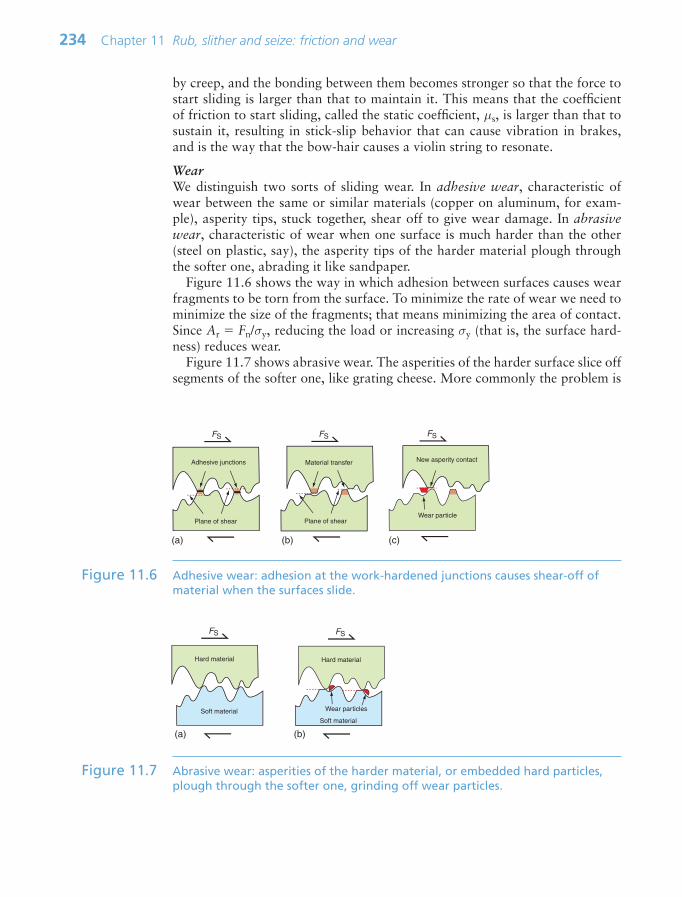
by creep, and the bonding between them becomes stronger so that the force tostart sliding is larger than that to maintain it. This means that the coefficient of friction to start sliding, called the static coefficient, µs, is larger than that tosustain it, resulting in stick-slip behavior that can cause vibration in brakes,and is the way that the bow-hair causes a violin string to resonate.
WearWe distinguish two sorts of sliding wear. In adhesive wear, characteristic ofwear between the same or similar materials (copper on aluminum, for exam-ple), asperity tips, stuck together, shear off to give wear damage. In abrasivewear, characteristic of wear when one surface is much harder than the other(steel on plastic, say), the asperity tips of the harder material plough throughthe softer one, abrading it like sandpaper.
Figure 11.6 shows the way in which adhesion between surfaces causes wearfragments to be torn from the surface. To minimize the rate of wear we need tominimize the size of the fragments; that means minimizing the area of contact.Since Ar Fn/σy, reducing the load or increasing σy (that is, the surface hard-ness) reduces wear.
Figure 11.7 shows abrasive wear. The asperities of the harder surface slice offsegments of the softer one, like grating cheese. More commonly the problem is
234 Chapter 11 Rub, slither and seize: friction and wear
FS
Adhesive junctions
Plane of shear
FS
New asperity contact
FS
Material transfer
Plane of shearWear particle
(a) (b) (c)
Figure 11.6 Adhesive wear: adhesion at the work-hardened junctions causes shear-off ofmaterial when the surfaces slide.
Hard material
Soft material
FS
Hard material
Soft material
FS
Wear particles
(a) (b)
Figure 11.7 Abrasive wear: asperities of the harder material, or embedded hard particles,plough through the softer one, grinding off wear particles.
Ch11-H8391.qxd 1/16/07 6:05 PM Page 234

one of contamination: hard particles that sneak into the surface—dust, sand,oxidized wear particles—embed themselves in one surface and plough throughthe other. It is to prevent this that cars have air and oil filters.
11.5 Design and selection: materials to manage friction and wear
Bearings allow two components to move relative to each other in one or twodimensions while constraining them in the others. The key criteria are low fric-tion coupled with the ability to support the bearing load Fn without yielding,overheating or wearing excessively. Brakes and clutches, by contrast, rely onhigh friction, but there is more to their design than that, as we shall see in amoment. But first, bearings.
Dry sliding, as we have seen, generally leads to friction with a coefficient µ ofabout 0.5. If the bearings of the drive-train of your car had a µ of this magni-tude, negligible power would reach the wheels—almost all would be lost asheat in the bearing surfaces. In reality, about 15% of the power of the engine islost in friction because of two innovations: lubrication and the replacement ofsliding by rolling bearings.
LubricationMost lubricants are viscous oils containing additives with polar groups (fattyacids with –OH groups not unlike ordinary soap) that bind to metal surfacesto create a chemisorbed boundary layer (Figure 11.8). A layer of the lubricantbetween the surfaces allows easy shear, impeded only by the viscosity of the oil,giving a coefficient of fraction in the range 0.001–0.01. When the sliding sur-faces are static, the bearing load Fn tends to squeeze the oil out of the bearing,but the bonding of the additive is strong enough to resist, leaving the two sur-faces separated by a double-layer of lubricating molecules. This boundary-layerlubrication is sufficient to protect the surfaces during start-up and sliding atlow loads, but it is not something to rely on for continuous use or high per-formance. For this you need hydrodynamic lubrication.
11.5 Design and selection: materials to manage friction and wear 235
Fn
Chemisorbed monolayersof polar molecules
Figure 11.8 The formation of a boundary layer of chemisorbed, polar molecules; the red dotrepresents the polar group, the tail the hydrocarbon chain attached to it.
Ch11-H8391.qxd 1/16/07 6:05 PM Page 235

The viscosity of the oil is both a curse and a blessing—a curse because it exertsa drag (and thus friction) on the sliding components; a blessing because, with-out it, hydrodynamic lubrication would not be possible. Figure 11.9 explains(an explanation first provided by Reynolds4). Sliding bearings are designed sothat the surfaces are slightly inclined. Oil is dragged along the wedge-shapedregion between them from the wide to the narrow end, as in Figure 11.9(a).The rise in pressure as the oil is compressed forces the surfaces apart against theforce of the normal load carried by the bearing. The maximum pressure isreached just behind the center of the slider, where the color is most intense inthe figure. The same principle governs the self-alignment of a rotating journalbearing, as in Figure 11.9(b). Again, the lubricant is dragged by viscosity intothe wide end of the wedge-shaped region and swept towards the narrow end,where the rise of pressure pushes the journal back onto the axis of the bearing.The result is that the surfaces never touch but remain separated by a thin filmof oil or other lubricating fluid.
236 Chapter 11 Rub, slither and seize: friction and wear
Oil film Slider
Pre
ssur
e
Distance(a)
Pre
ssur
e
Radial distance
Oil film
(b)
Figure 11.9 The distribution of pressure under a sliding and a rotating bearing withhydrodynamic lubrication.
4 Osborne Reynolds (1842–1912), Northern Irishman, brilliant mathematician and engineerbut awful lecturer, known for his contributions to lubrication, turbulence and for hiscelebrated Number—the dimensionless group describing the transition from laminar toturbulent flow.
Ch11-H8391.qxd 1/16/07 6:05 PM Page 236

At high temperatures, hydrocarbon lubricants decompose. Solid lubricants—PTFE, molybdenum disulfide (MoS2) and graphite (one form of carbon)—extend the operating temperature to 500°C. PTFE, good to about 250°C, hasan intrinsically low coefficient of friction. Moly-disulfide (up to 300°C) andgraphite (to 500°C) rely on their lamellar (layer-like) crystal structure, able toshear easily on certain crystal planes, to provide coefficients of friction well below0.1. All these can be applied as lubricants or incorporated into the pores ofporous bearings (made by sintering powdered metal like bronze and cast iron)to give self-lubricating bearings.
That’s the background. So what materials are good for bearings? Thatdepends—plane bearings or roller bearings?
Plane bearingsThe surfaces of sliding bearings, if properly lubricated, do not touch. Thenalmost any material that meets the other constraints of the design will do—steel,cast iron, brass, bronze. The key material properties are strength (to carry thebearing loads), corrosion resistance and conformability—the ability to adapt toslight misalignment. Full hydrodynamic lubrication breaks down under staticloads or when sliding velocities are small, and long-term reliance on boundarylubrication is risky. Bearing materials are designed to cope with this.
When soft metals slide over each other (lead on lead, for instance), the junc-tions are weak but their area of contact is large so µ is large. When hard met-als slide (e.g. steel on steel), the junctions are small but they are strong, and againµ is large. The way to get low friction with high strength is to support a softmetal with a hard one, giving weak junctions of small area. White-metal bear-ings, for example, consist of soft lead or tin supported in a matrix of a strongermaterial; leaded-bronze bearings consist of a matrix of strong, corrosion-resistantbronze containing particles of soft lead that smear out to give an easily shearedsurface film when asperities touch; polymer-impregnated porous bearings aremade by partly sintering bronze and then forcing a polymer (usually PTFE) intoits pores. Bearings like these are not designed to run dry, but if they do, the softcomponent saves them, at least for a while.
Rolling bearingsIn rolling element bearings the load is carried by a set of balls or rollers trappedbetween an inner and an outer race by a cage, as in Figure 11.10. When theloading is radial the load is carried at any instant by half the balls or rollers, butnot equally: the most heavily loaded one carries about 5/Z times the appliedload, where Z is the total number of balls or rollers in the bearing. Its contactarea with the race is small, so the contact stresses are high.
The main requirement is that the deformation of the components of the bear-ing remain at all times elastic, so the criterion for material choice is that of highhardness. That usually means a high-carbon steel or a tool steel. If the environ-ment is corrosive or the temperature high, stainless steel or ceramic (silicon car-bide or silicon nitride) are used. When the loads are very light the races can be
11.5 Design and selection: materials to manage friction and wear 237
Ch11-H8391.qxd 1/16/07 6:05 PM Page 237
made from thermoplastic—polypropylene or acetal—with the advantage thatno lubrication is needed (cheap bike pedals sometimes have such bearings).
When rolling element bearings fail, it is usually because of fatigue—therepeated loading and unloading of ball and race as the bearing rotates causescracks to nucleate, splitting the balls or pitting the races. Inclusions in the mate-rial are sources of fatigue cracks, so steels for rolling bearings are processed tobe as clean and inclusion free as possible by processing under vacuum.
High friction: materials for brakes and clutches
Applying friction sounds easy—just rub. Brakes for horse-drawn carriages didjust that—spoon-shaped blocks of wood, sometimes faced with leather (bigger µ),were wound down with a screw to rub on the rim of the carriage wheel. Butbrake materials today do much more.
The friction coefficient of materials for brake linings is—surprisingly—notspecial: µ is about 0.4. The key thing is not µ but the ability to apply it withoutvibration, wear or fade. That is not easy when you reckon that, to stop a one-tonne car from 100 kph (60 mph) requires that you find somewhere to put about0.4 MJ. That’s enough (if you don’t lose any) to heat 1 kg of steel to 800°C.Brake materials must apply friction at temperatures that can approach suchvalues, and they must do so consistently and without the stick-slip that causes‘brake squeal’—not acceptable in even the cheapest car. That means materialsthat can tolerate heat, conduct it away to limit temperature rise and—curiously—lubricate, since it is this that quenches squeal.
For most of the history of the automobile, brake linings were made of com-pacted asbestos (able to tolerate 2000°C ) mixed with brass or copper particlesor wires for heat conduction and strength. When it became apparent thatasbestos dust—the product of brake wear—was perhaps not so good for you,new materials appeared. They are an example of hybrid material design meth-ods: no one material can do what you want, so we synthesize one that does.
Today’s materials are a synthesis: a matrix, an abrasive additive to increasefriction, a reinforcement—one to help conduct heat if possible—and a lubricant
238 Chapter 11 Rub, slither and seize: friction and wear
Ball
Inner race
Outer race
Cage
Contactstress
Figure 11.10 A rolling-contact bearing. The contact stresses are high, requiring materials withhigh hardness and resistance to fatigue failure.
Ch11-H8391.qxd 1/16/07 6:05 PM Page 238

to suppress vibration. Intimate details are trade secrets, but here is the idea. Thebrake pads on your bike are made up of a synthetic rubber with particles of acheap silicate to reduce pad wear and give wet friction. Those on your car havea phenolic matrix with particles of silicates, silicon carbide (sandpaper grit) tocontrol friction and graphite or MoS2 as a lubricant. Those on a military jet, a747 or an F1 car are carbon or ceramic—here high temperature is the problem;replacement every 10 days is acceptable if they stand the heat (try calculatinghow much aluminum you could melt with the energy dissipated in bringing a200-tonne 747 to rest from 200 kph).
Waging war on wearAs explained earlier, the rate of wear increases with the bearing pressure P(equation (11.4)). It also increases with sliding velocity v because the faster thesliding, the more work is done against friction and it all turns into heat. A givenbearing material has an acceptable P–v envelope within which it is usable; ven-ture outside it and seizure or catastrophic wear awaits you (Figure 11.11(a)). Toextend the envelope upwards, we select materials with higher strength; toextend it laterally, we choose materials with higher thermal conductivity andmelting point—or lower friction.
Lubrication, of course, reduces friction. Figure 11.11(b) shows that this doesnot increase the admissible bearing pressure—that is a static property of thematerial—but it does increase the permissible sliding velocity. Boundary lubri-cation expands the envelope a little; hydrodynamic lubrication expands itmuch more—but note its drop-off at low velocities because there is not enoughsliding speed to build up the pressure profiles of Figure 11.9.
At very high rotational velocities, approached in ultra-centrifuges, gyro-scopic navigation systems and super-flywheels for energy storage, there is an
11.5 Design and selection: materials to manage friction and wear 239
0.01
0.1
1
10
100
1000
0.01 0.1 1 10 100Sliding velocity v (m/s)
Bea
ring
pres
sure
P (
MP
a)
1000 10 000
Dry sliding
Boundarylubrication
Full hydrodynamiclubrication
Burst velocity
0.01
0.1
1
10
100
1000
0.01 0.1 1 10 100
Sliding velocity v (m/s)
Bea
ring
pres
sure
P (
MP
a)
(a) (b)
Safe usearea
Pressure limitedby yield
Velocity limitedby overheating
Figure 11.11 (a) A P–v curve for a bearing material. (b) P–v envelopes for various lubricatedand unlubricated sliding, ultimately limited by the disintegration of the bearingunder centrifugal force at very high velocities.
Ch11-H8391.qxd 1/16/07 6:05 PM Page 239
ultimate cut-off. It is the speed at which centrifugal forces exceed the strengthof the material and the whole system disintegrates.
Hard materials have low wear rates but they tend to be brittle. Soft ones aretougher but they wear rapidly. Wear is a surface property, toughness a propertyof the bulk. So the way to fight wear is to take a tough material and give it ahard surface coating, using techniques of surface treatment. High-carbon steelsare surface hardened by rapidly heating with a flame, an electron beam or alaser beam and then quenching the surface. Carburizing, nitriding and boridinggive wear resistance to components like crankshafts or ball races by diffusingcarbon, nitrogen or boron atoms into a thin surface layer, where they react togive particles of carbides, nitrides or borides. Hard, corrosion-resistant layersof alloys rich in tungsten, cobalt or chromium can be sprayed onto surfaces,but a refinishing process is then necessary to restore dimensional precision.Hard ceramic coatings of alumina (Al2O3) or of tungsten or titanium carbide(WC, TiC) can be applied by plasma spraying to give both wear resistance andresistance to chemical attack, and chemical and physical vapor deposition meth-ods allow surface coatings of other metals and ceramics, including diamond-like carbon.
Records for all these treatments (and more) are contained in the CES soft-ware under the heading ‘Surface treatment’. The software allows selection ofcoatings to meet given design requirements, of which wear resistance is one ofthe more important. We return to these in Chapter 18 on selecting processes.
11.6 Summary and conclusions
When surfaces slide, there is friction and there is wear. Eliminate all frictionand a spinning wheel would spin forever. Eliminate all wear and it would lastforever too. Both are about as probable as living forever while eating nothing.So we have to learn to live with them: to use them when they are useful, to min-imize the problems they cause when they are a nuisance.
The remarkable thing about friction is that, if you slide one surface overanother, the force to do so depends only on the normal force pushing the sur-faces together, not on the area of the surface. That is because surfaces are notperfectly smooth; they touch only at points (flattened a little by the pressure)—just enough of them to support the normal force. Changing the area does notchange the number of contact points. The sliding force is the force to shear thecontact points, so it, too, is independent of area.
The points of contact are where wear happens. When surfaces slide thepoints shear off, becoming wear particles. This process can be useful—it helpssurfaces bed down and conform by what is called ‘run-in’. But if the wear par-ticles or particles from elsewhere (dust, grit) get between the surfaces, thegrinding action continues and the surfaces wear.
Soft materials—lead, polyethylene, PTFE, graphite—shear easily. Impregnatinga sliding material with one of these reduces friction—skis and snow boards
240 Chapter 11 Rub, slither and seize: friction and wear
Ch11-H8391.qxd 1/16/07 6:05 PM Page 240

have polyethylene surfaces for just this reason. Better still is hydrodynamiclubrication: floating the sliding surfaces apart by dragging fluid between them.Flotation requires that the surfaces slide; if they stop the fluid is squeezed out.Clever lubricants overcome this by bonding to the surfaces, leaving a thin bound-ary layer that is enough to separate the surfaces until hydrodynamic lubricationgets going.
Friction, wear and corrosion cause more damage to mechanisms than any-thing else. They are the ultimate determinants of the life of products—or theywould be, if we kept them until they wore out. But in today’s society, manyproducts are binned before they are worn out; many when they still work per-fectly well. More on that subject in Chapter 20.
11.7 Further reading
Bowden, F.P. and Tabor, D. (1950 and 1964) The Friction and Lubrication of Solids,Parts 1 and 2, Oxford, University Press, Oxford, UK. ISBN 0-19-851204-X. (Twovolumes that establish the cornerstones of tribology: contact between solids; frictionof metals and non-metals; frictional temperature rise; boundary lubrication and otherchemical effects; adhesion; sliding wear; and hardness.)
Hutchings, I.M. (1992) Tribology: Friction and Wear of Engineering Materials, Arnold,London, UK. ISBN 0-340-56184-X. (An introduction to the mechanics and materialsscience of friction, wear and lubrication.)
Neale, M.J. (1995) The Tribology Handbook, 2nd edition, Butterworth-Heinemann,Oxford, UK. ISBN 0-7506-1198-7. (A tribological bible: materials, bearings, drives,brakes, seals, lubrication failure and repair.)
11.8 Exercises
11.8 Exercises 241
Exercise E11.1 Define the coefficient of friction. Explain why it is independent of the area ofcontact of the sliding surfaces.
Exercise E11.2 Woods—both resinous wood from the pine family and hardwoods likelignum vitae (it is so dense it sinks in water)—were, historically, used forbearings; even clocks had hardwood bearings. Why? Think of your ownideas, then research the Web.
Exercise E11.3 Give examples, based on your experience in sport (tennis, golf, swimming,skiing, rock climbing, hang-gliding, etc.) of instances in which friction iswanted and when it is not.
Exercise E11.4 Now a more challenging one. Do the same, based again on your experiencein sport, of instances in which wear is desirable and in which it is not.
Exercise E11.5 What are the characteristics of materials that are a good choice for use asbrake pads?
Ch11-H8391.qxd 1/16/07 6:05 PM Page 241

242 Chapter 11 Rub, slither and seize: friction and wear
Exercise E11.6 A 30 mm diameter plane bearing of length 20 mm is to be made of a materialwith the P – v characteristics shown in Figure 11.11 (b). If the bearing loadis 300 N and the maximum rotation rate is 500 rpm, is it safe to run it dry?If not, is boundary lubrication sufficient? (Remember that the bearing pres-sure is the load divided by the projected area normal to the load.)
Exercise E11.7 A bronze statue weighing 4 tonnes with a base of area 0.8 m2 is placed on agranite museum floor. The yield strength of the bronze is 240 MPa. What isthe true area of contact, Ar, between the base and the floor?
Exercise E11.8 The statue of the previous example was moved to a roof courtyard with alead floor. The yield strength of the lead is 6 MPa. What now is the true areaof contact?
Exercise E11.9 How would you measure the true area of contact Ar between two surfacespressed into contact? Use your imagination to devise ways.
Ch11-H8391.qxd 1/16/07 6:05 PM Page 242

11.9 Exploring design with CES 243
11.9 Exploring design with CES (use Level 2 unless otherwise stated)
Exercise E11.10 Use the ‘Search’ facility to find materials that are used as ball bearings.(Search on the singular—ball bearing—since that picks up the plural as well.)
Exercise E11.11 Use the ‘Search’ facility to find materials that are used as for brake pads. Dothe same for brake discs.
Exercise E11.12 Use a ‘Limit’ selection stage applied to the Surface Treatment data table tofind processes that enhance wear resistance. (To do this, click on ‘Select’ inthe main toolbar, then on ‘Selection Data’, just below it. Select Level 2Surface treatment in the dialog box. Open a ‘Limit’ stage, open Function oftreatment, and click on Wear resistance.) Explore the record for laser-basedmethods. What are its typical uses?
Exercise E11.13 Follow the same procedure as that of the previous example to search forprocesses used to control friction. Explore the record for grinding andmechanical polishing. What are grinding wheels made of?
Ch11-H8391.qxd 1/16/07 6:05 PM Page 243

Ch11-H8391.qxd 1/16/07 6:05 PM Page 244

Chapter 12Agitated atoms:
materials and heat
Chapter contents
12.1 Introduction and synopsis 24612.2 Thermal properties: definition and
measurement 24612.3 The big picture: thermal property
charts 24912.4 Drilling down: the physics of
thermal properties 25112.5 Manipulating thermal properties 25712.6 Design to exploit thermal properties 25812.7 Summary and conclusions 26812.8 Further reading 26912.9 Exercises 27012.10 Exploring design with CES 27112.11 Exploring the science with
CES Elements 272
A heat exchanger. (Image courtesy of theInternational Copper Development Association)
Ch12-H8391.qxd 1/16/07 6:07 PM Page 245
246 Chapter 12 Agitated atoms: materials and heat
12.1 Introduction and synopsis
Thermal properties quantify the response of materials to heat. Heat, untilabout 1800, was thought to be a physical substance called ‘caloric’ that somehowseeped into things when they were exposed to flame. It took the AmericanBenjamin Thompson1, backed up by none other than the formidable Carnot2, tosuggest what we now know to be true: that heat is atoms or molecules in motion.In gases, they are flying between occasional collisions with each other. In solids,by contrast, they vibrate about their mean positions; the higher the temperature,the greater the amplitude of vibrations. From this perception emerges all of ourunderstanding of thermal properties of solids: their heat capacity, expansioncoefficient, conductivity, even melting.
Heat affects mechanical and physical properties too. As temperature rises,materials expand, the elastic modulus decreases, the strength falls and thematerial starts to creep, deforming slowly with time at a rate that increases asthe melting point is approached until, on melting, the solid loses all stiffnessand strength. This we leave for Chapter 13.
Thermal design, the ultimate topic of this chapter, is design to cope properlywith the effects of heat or, where possible, to exploit them. The chapter open-ing page shows an example: a copper heat exchanger, designed to transfer heatefficiently between two circulating fluids.
12.2 Thermal properties: definition and measurement
Two temperatures, the melting temperature, Tm, and the glass temperature, Tg(units for both: kelvin3, K, or centigrade, °C) are fundamental points of refer-ence because they relate directly to the strength of the bonds in the solid.Crystalline solids have a sharp melting point, Tm. Non-crystalline solids do not;the glass temperature Tg characterizes the transition from true solid to very vis-cous liquid. It is helpful, in engineering design, to define two further tempera-tures: the maximum and minimum service temperatures, Tmax and Tmin (unitsfor both: K or °C). The first tells us the highest temperature at which the mate-rial can be used continuously without oxidation, chemical change or excessive
1 Benjamin Thompson (1753–1814), later Lord Rumford, while in charge of the boring ofcannons at the Watertown Arsenal near Boston, Mass., noted how hot they became andformulated the ‘mechanical equivalent of heat’—what we now call the heat capacity.
2 Sadi Nicolas Léonhard Carnot (1796–1832), physicist and engineer, formulator of theCarnot cycle and the concept of entropy, the basis of the optimization of heat engines. Hedied of cholera, a fate most physicists today are, mercifully, spared.
3 William Thompson, Lord Kelvin (1824–1907), Scottish mathematician who contributed tomany branches of physics; he was known for a self-confidence that led him to claim (in1900) that there was nothing more to be discovered in physics—he already knew it all.
Ch12-H8391.qxd 1/16/07 6:07 PM Page 246
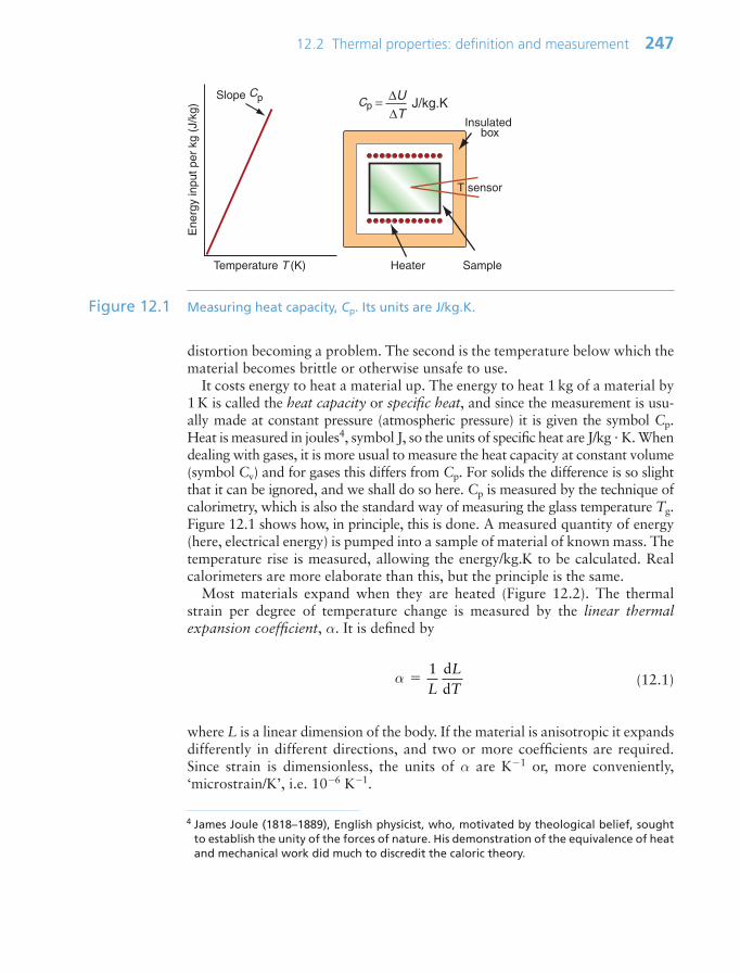
12.2 Thermal properties: definition and measurement 247
Temperature T (K)
Slope Cp
Ene
rgy
inpu
t per
kg
(J/k
g)
Cp∆U∆T
Heater Sample
Insulated box
T sensor
J/kg.K=
Figure 12.1 Measuring heat capacity, Cp. Its units are J/kg.K.
distortion becoming a problem. The second is the temperature below which thematerial becomes brittle or otherwise unsafe to use.
It costs energy to heat a material up. The energy to heat 1 kg of a material by1 K is called the heat capacity or specific heat, and since the measurement is usu-ally made at constant pressure (atmospheric pressure) it is given the symbol Cp.Heat is measured in joules4, symbol J, so the units of specific heat are J/kg K. Whendealing with gases, it is more usual to measure the heat capacity at constant volume(symbol Cv) and for gases this differs from Cp. For solids the difference is so slightthat it can be ignored, and we shall do so here. Cp is measured by the technique ofcalorimetry, which is also the standard way of measuring the glass temperature Tg.Figure 12.1 shows how, in principle, this is done. A measured quantity of energy(here, electrical energy) is pumped into a sample of material of known mass. Thetemperature rise is measured, allowing the energy/kg.K to be calculated. Realcalorimeters are more elaborate than this, but the principle is the same.
Most materials expand when they are heated (Figure 12.2). The thermalstrain per degree of temperature change is measured by the linear thermalexpansion coefficient, α. It is defined by
(12.1)
where L is a linear dimension of the body. If the material is anisotropic it expandsdifferently in different directions, and two or more coefficients are required.Since strain is dimensionless, the units of α are K1 or, more conveniently,‘microstrain/K’, i.e. 106 K1.
α 1L
LT
dd
4 James Joule (1818–1889), English physicist, who, motivated by theological belief, soughtto establish the unity of the forces of nature. His demonstration of the equivalence of heatand mechanical work did much to discredit the caloric theory.
Ch12-H8391.qxd 1/16/07 6:07 PM Page 247

Power is measured in watts5; 1 watt (W) is 1 joule/second. The rate at whichheat is conducted through a solid at steady-state (meaning that the temperatureprofile does not change with time) is measured by the thermal conductivity, λ(units: W/m.K). Figure 12.3 shows how it is measured: by recording the heatflux q (W/m2) flowing through the material from a surface at higher temperature
248 Chapter 12 Agitated atoms: materials and heat
Temperature change ∆T (K)
Slope α
The
rmal
str
ain
ε =
δL
/L
Insulation
HeaterSample
∆L
L
α = ∆L∆TL
1 K1
Figure 12.2 Measuring the thermal expansion coefficient, α. Its units are 1/K or, moreusually, 106/K (microstrain/K).
Hea
t flu
x q
(W
/m2 )
T-gradient (T1 T2)/X (K/m)
Slope λ
Insulation Sample
Heatinput
q W/m2
Heatsink
q W/m2
T1 T2
X
∆Tq = λ ∆X
W/m2
Figure 12.3 Measuring the thermal conductivity, λ. Its units are W/m K.
5 James Watt (1736–1819), instrument maker and inventor of the condenser steam engine(the idea came to him whilst ‘walking on a fine Sabbath afternoon’), which he doggedlydeveloped. Unlike so many of the characters footnoted in this book, Watt, in his finalyears, was healthy, happy and famous.
Ch12-H8391.qxd 1/16/07 6:07 PM Page 248

T1 to a lower one at T2 separated by a distance x. The conductivity is calculatedfrom Fourier’s6 law:
(12.2)
(where q is the heat flux per unit area (units: W/m2))Thermal conductivity, as we have said, governs the flow of heat through a mate-
rial at steady-state. The property governing transient heat flow (when temperaturevaries with time) is the thermal diffusivity, a (units: m2/s). The two are related by
(12.3)
where ρ is the density and Cp is, as before, the heat capacity. The thermal diffusiv-ity can be measured directly by measuring the time it takes for a temperature pulseto traverse a specimen of known thickness when a heat source is applied briefly tothe one side; or it can be calculated from λ (and ρCp) via equation (12.3).
12.3 The big picture: thermal property charts
Three charts give an overview of thermal properties and their relationship tostrength.
Thermal expansion, α, and thermal conductivity, λFigure 12.4 maps thermal expansion, α, and thermal conductivity, λ. Metalsand technical ceramics lie towards the lower right: they have high conductivi-ties and modest expansion coefficients. Polymers and elastomers lie at theupper left: their conductivities are 100 times less and their expansion coeffi-cients 10 times greater than those of metals. The chart shows contours of λ/α,a quantity important in designing against thermal distortion—a subject wereturn to in Section 12.6. An extra material, Invar (a nickel alloy), has beenadded to the chart because of its uniquely low expansion coefficient at and nearroom temperature, a consequence of a trade-off between normal expansionand a contraction associated with a magnetic transformation.
Thermal conductivity, λ, and thermal diffusivity, aFigure 12.5 shows the room temperature values of thermal conductivity, λ, andthermal diffusivity, a, with contours of volumetric heat capacity ρCp, equal tothe ratio of the two, λ/α (from equation (12.3)). The data span almost fivedecades in λ and a. Solid materials are strung out along the line
aC
λ
ρ p
qTx
T T
x
λ λ
dd
( )1 2
12.3 The big picture: thermal property charts 249
6 Baron Jean Baptiste Joseph Fourier (1768–1830), mathematician and physicist; he nearlycame to grief during the French Revolution but survived to become one of the savantswho accompanied Napoleon Bonaparte in his conquest of Egypt.
Ch12-H8391.qxd 1/16/07 6:07 PM Page 249
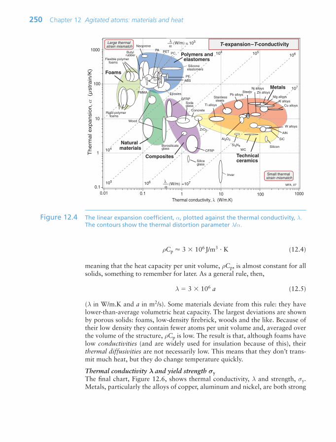
ρCp 3 106J/m3 K (12.4)
meaning that the heat capacity per unit volume, ρCp, is almost constant for allsolids, something to remember for later. As a general rule, then,
λ 3 106 a (12.5)
(λ in W/m.K and a in m2/s). Some materials deviate from this rule: they havelower-than-average volumetric heat capacity. The largest deviations are shownby porous solids: foams, low-density firebrick, woods and the like. Because oftheir low density they contain fewer atoms per unit volume and, averaged overthe volume of the structure, ρCp is low. The result is that, although foams havelow conductivities (and are widely used for insulation because of this), theirthermal diffusivities are not necessarily low. This means that they don’t trans-mit much heat, but they do change temperature quickly.
Thermal conductivity λ and yield strength σyThe final chart, Figure 12.6, shows thermal conductivity, λ and strength, σy.Metals, particularly the alloys of copper, aluminum and nickel, are both strong
250 Chapter 12 Agitated atoms: materials and heat
Thermal conductivity, λ (W/m.K)
0.01
Therm
al e
xpansi
on,
α (µ
stra
in/K
)
0.1
10.1 10 100 1000
1
10
100
1000
= 103Large thermal strain mismatch
Small thermal strain mismatch
λα
(W/m)
λα
(W/m)
104 105106
106
107
=107
104
105
Foams
Polymers and elastomers
Metals
Technicalceramics
Composites
Natural materials
W alloys
Steels
Ti alloys
Mg alloys
CFRP
GFRPAl alloys
Rigid polymer foams
Flexible polymer foams
Ni alloys
Cu alloys
Zn alloys
PA
PMMA
PCPET
Wood
Butyl rubber
Silicone elastomers
Concrete
WC
Al2O3 SiC
Si3N4
T- expansion –T- conductivity
Pb alloysStainless steels
Silicaglass
Silicon
AlN
Sodaglass
Neoprene
PE
Epoxies
ABS
MFA, 07
Invar
Borosilicateglass
ZrO2
Figure 12.4 The linear expansion coefficient, α, plotted against the thermal conductivity, λ.The contours show the thermal distortion parameter λ/α.
Ch12-H8391.qxd 1/16/07 6:07 PM Page 250
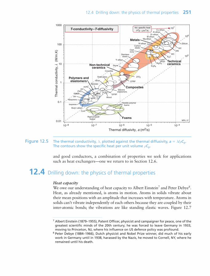
12.4 Drilling down: the physics of thermal properties 251
Thermal diffusivity, a (m2/s)
The
rmal
con
duct
ivity
, λ (
W/m
.K)
10−8 10−7 10−6 10−5 10−4
0.01
0.1
1
10
100
1000107
106
105
Vol. specific heatρCp (J/m3.K)
Foams
Polymers and elastomers
Metals
Technicalceramics
Composites
Lead alloys
W alloys
Carbon steels
Ti alloys
Mg alloys
CFRP
GFRP
Al alloys
Rigid polymer foams
Flexible polymer foams
Ni alloys
Cu alloys
Zn alloys
PTFEPC
Cork
Wood
Butyl rubber
Silicone elastomers
Concrete
Al2O3
SiC
Si3N4
T-conductivity –T-diffusivity
B4C
PP
Isoprene
Non-technical ceramics
MFA, 07
Cast irons
WC
Soda glass
Stone
Brick
Epoxies
Stainless steels
AlN
Silicon
Neoprene
PMMAPVC
ZrO2
Figure 12.5 The thermal conductivity, λ, plotted against the thermal diffusivity, a λ/ρCp.The contours show the specific heat per unit volume ρCp.
and good conductors, a combination of properties we seek for applicationssuch as heat exchangers—one we return to in Section 12.6.
12.4 Drilling down: the physics of thermal properties
Heat capacityWe owe our understanding of heat capacity to Albert Einstein7 and Peter Debye8.Heat, as already mentioned, is atoms in motion. Atoms in solids vibrate abouttheir mean positions with an amplitude that increases with temperature. Atoms insolids can’t vibrate independently of each others because they are coupled by theirinter-atomic bonds; the vibrations are like standing elastic waves. Figure 12.7
7 Albert Einstein (1879–1955), Patent Officer, physicist and campaigner for peace, one of thegreatest scientific minds of the 20th century; he was forced to leave Germany in 1933,moving to Princeton, NJ, where his influence on US defence policy was profound.
8 Peter Debye (1884–1966), Dutch physicist and Nobel Prize winner, did much of his earlywork in Germany until in 1938, harassed by the Nazis, he moved to Cornell, NY, where heremained until his death.
Ch12-H8391.qxd 1/16/07 6:07 PM Page 251

252 Chapter 12 Agitated atoms: materials and heat
Yield strength, σy (MPa)0.01 0.1 1 10 100 1000
The
rmal
con
duct
ivity
, λ (
W/m
.K)
0.01
0.1
1
10
100
1000
MFA 07
Foams
Polymers
Metals
Technical ceramics
Composites
Natural materials
Lead alloys
W alloys
Carbon steels
Ti alloys
Mg alloys
CFRP
GFRP
Al alloys
Rigid polymer foams
Flexible polymer foams
Cu alloys
Zn alloys
PA
PMMAPET
Cork
Wood
Butyl rubber
Concrete
Tungstencarbide
Al2O3
SiC
Si3N4
T-Conductivity –Strength
Stainless steels
Al nitrideSilicon
PP PS
PE
Neoprene
Stone
Soda glass
Ni basedsuperalloys
Elastomers
Non-technical ceramics
ZrO2
PC
Cement
Brick
Figure 12.6 Thermal conductivity λ and strength σy.
a(b)
(a)
(c)
(d)
Figure 12.7 (a) An atom vibrating in the ‘cage’ of atoms that surround it with three degrees offreedom. (b) A row of atoms at rest. (c) A longitudinal wave. (d) One of twotransverse waves (in the other the atoms oscillate normal to the page).
Ch12-H8391.qxd 1/16/07 6:07 PM Page 252
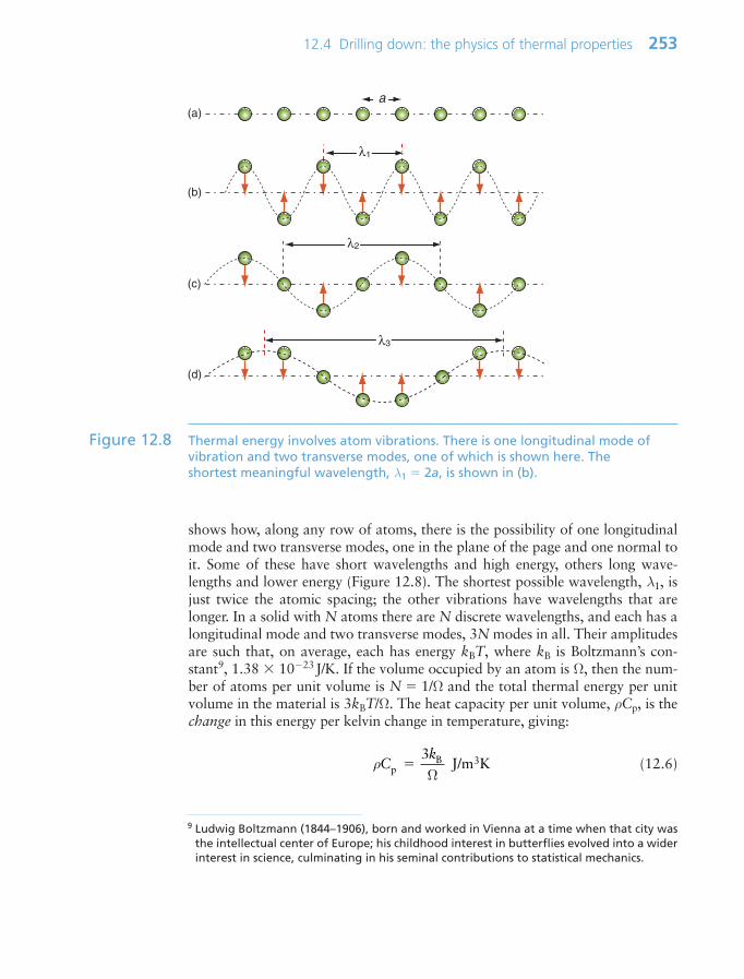
shows how, along any row of atoms, there is the possibility of one longitudinalmode and two transverse modes, one in the plane of the page and one normal toit. Some of these have short wavelengths and high energy, others long wave-lengths and lower energy (Figure 12.8). The shortest possible wavelength, λ1, isjust twice the atomic spacing; the other vibrations have wavelengths that arelonger. In a solid with N atoms there are N discrete wavelengths, and each has alongitudinal mode and two transverse modes, 3N modes in all. Their amplitudesare such that, on average, each has energy kBT, where kB is Boltzmann’s con-stant9, 1.38 1023J/K. If the volume occupied by an atom is Ω, then the num-ber of atoms per unit volume is N 1/Ω and the total thermal energy per unitvolume in the material is 3kBT/Ω. The heat capacity per unit volume, ρCp, is thechange in this energy per kelvin change in temperature, giving:
(12.6)ρCk
pB J/m K
3 3
Ω
12.4 Drilling down: the physics of thermal properties 253
a
λ1
λ2
λ3
(a)
(b)
(c)
(d)
Figure 12.8 Thermal energy involves atom vibrations. There is one longitudinal mode ofvibration and two transverse modes, one of which is shown here. The shortest meaningful wavelength, λ1 2a, is shown in (b).
9 Ludwig Boltzmann (1844–1906), born and worked in Vienna at a time when that city wasthe intellectual center of Europe; his childhood interest in butterflies evolved into a widerinterest in science, culminating in his seminal contributions to statistical mechanics.
Ch12-H8391.qxd 1/16/07 6:07 PM Page 253

Atomic volumes do not vary much; all lie within a factor of 3 of the value2 1029/m3, giving a volumetric heat capacity
(12.7)
The chart of Figure 12.5 showed that this is indeed the case.
Thermal expansionIf a solid expands when heated (and almost all do) it must be because the atoms aremoving further apart. Figure 12.9 shows how this happens. It looks very like anearlier one, Figure 4.22, but there is a subtle difference: the force–spacing curve, astraight line in the earlier figure, is not in fact quite straight; the bonds becomestiffer when the atoms are pushed together and less stiff when they are pulledapart. Atoms vibrating in the way described earlier oscillate about a mean spacingthat increases with the amplitude of oscillation, and thus with increasing temper-atures. So thermal expansion is a nonlinear effect; if the bonds between atomswere linear springs, there would be no expansion.
ρCp J/m K≈ 2 106 3
254 Chapter 12 Agitated atoms: materials and heat
Force F
Spacing, a
Spacing, a ao
Springstiffness S
Energy U
Tension
Compression
Thermal oscillationsEnergy U = F dδ
Mean spacingof oscillatingatoms at T1
Mean spacing, a
Increasingtemperature
To
T1
T2
T3
Figure 12.9 Thermal expansion results from the oscillation of atoms in an unsymmetricalenergy well.
Ch12-H8391.qxd 1/16/07 6:07 PM Page 254

The stiffer the springs, the steeper is the force–displacement curve and the nar-rower is the energy well in which the atom sits, giving less scope for expansion.Thus, materials with high modulus (stiff springs) have low expansion coeffi-cient, those with low modulus (soft springs) have high expansion—indeed, to agood approximation
(12.8)
(E in GPa, α in K1). It is an empirical fact that all crystalline solids expand byabout the same amount on heating from absolute zero to their melting point: itis about 2%. The expansion coefficient is the expansion per degree kelvin,meaning that
(12.9)
For example, tungsten, with a melting point of around 3330°C (3600 K) hasα 5 106/°C, while lead, with a melting point of about 330°C (600 K, six times lower) expands six times more (α 30 106/°C). Equation (12.9)(with Tm in kelvin, of course) is a remarkably good approximation for theexpansion coefficient. Note in passing that equations (12.8) and (12.9) indicatethat E is expected to scale with Tm—try exploring how well these approxima-tions hold using the CES Elements database.
Thermal conductivityHeat is transmitted through solids in three ways: by thermal vibrations; by themovement of free electrons in metals; and, if they are transparent, by radiation.Transmission by thermal vibrations involves the propagation of elastic waves.When a solid is heated the heat enters as elastic wave packets or phonons. Thephonons travel through the material and, like any elastic wave, they move withthe speed of sound, co(co E/ρ). If this is so, why does heat not diffuse at thesame speed? It is because phonons travel only a short distance before they arescattered by the slightest irregularity in the lattice of atoms through which theymove, even by other phonons. On average they travel a distance called themean free path, m, before bouncing off something, and this path is short: typ-ically less than 0.01 µm (108m).
We calculate the conductivity by using a net flux model, much as you wouldcalculate the rate at which cars accumulate in a car park by counting the rateat which they enter and subtracting the rate at which they leave. Phonon con-duction can be understood in a similar way, as suggested by Figure 12.10. Herea rod with unit cross-section carries a uniform temperature gradient dT/dxbetween its ends. Phonons within it have three degrees of freedom of motion(they can travel in the x, the y and the z directions). Focus on the midplaneM–M. On average, one-sixth of the phonons are moving in the x direction;
α ≈0 02.
mT
α 1 6 10 3.E
12.4 Drilling down: the physics of thermal properties 255
Ch12-H8391.qxd 1/16/07 6:07 PM Page 255
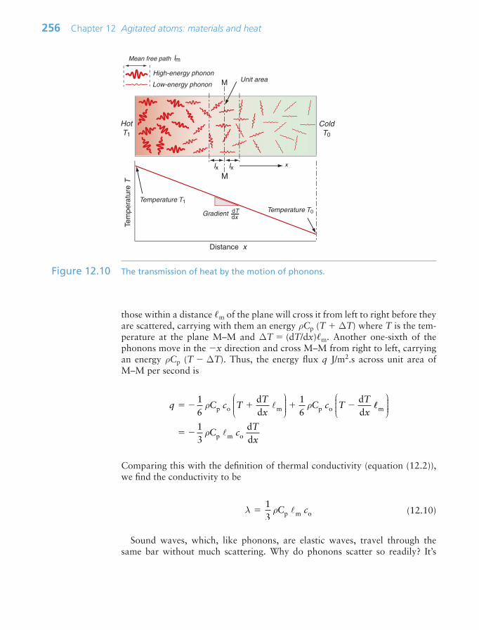
those within a distance m of the plane will cross it from left to right before theyare scattered, carrying with them an energy ρCp (T ∆T) where T is the tem-perature at the plane M–M and ∆T (dT/dx)m. Another one-sixth of thephonons move in the x direction and cross M–M from right to left, carryingan energy ρCp (T ∆T). Thus, the energy flux q J/m2.s across unit area ofM–M per second is
Comparing this with the definition of thermal conductivity (equation (12.2)),we find the conductivity to be
(12.10)
Sound waves, which, like phonons, are elastic waves, travel through thesame bar without much scattering. Why do phonons scatter so readily? It’s
λ ρ13 p m oC c
q C c TTx
C c TTx
16
ρ ρp o m p odd
16
dd
⎛
⎝⎜⎜⎜
⎞
⎠⎟⎟⎟⎟
m
p m o1 d
d
⎛
⎝⎜⎜⎜
⎞
⎠⎟⎟⎟⎟
3
ρC cTx
256 Chapter 12 Agitated atoms: materials and heat
High-energy phonon
Low-energy phonon
Mean free path
Unit area
Temperature T1
Distance x
Temperature T0
lxlx
lm
M
M
Gradient dTdx
x
Tem
pera
ture
THotT1
ColdT0
Figure 12.10 The transmission of heat by the motion of phonons.
Ch12-H8391.qxd 1/16/07 6:07 PM Page 256
because waves are scattered most by obstacles with a size comparable withtheir wavelengths—that is how diffraction gratings work. Audible sound waveshave wavelengths of meters, not microns; they are scattered by buildings(which is why you can’t always tell where a police siren is coming from) but notby the atom-scale obstacles that scatter phonons, with wavelengths starting attwo atomic spacings (Figure 12.8).
Elastic waves contribute little to the conductivity of pure metals such as cop-per or aluminum because the heat is carried more rapidly by the free electrons.Equation (12.10) still applies but now Cp, co and m become the thermal capac-ity, the velocity and the mean free path of the electrons. Free electrons also con-duct electricity, with the result that metals with high electrical conductivity alsohave high thermal conductivity (the Wiedemann–Franz law), as will be illus-trated in Chapter 14.
12.5 Manipulating thermal properties
Thermal expansionExpansion, as already mentioned, can generate thermal stress and cause distor-tion, undesirable in precise mechanisms and instruments. The expansion coef-ficient α, like modulus or melting point, depends on the stiffness and strengthof atomic bonds. There’s not much you can do about these, so the expansioncoefficient, normally, is beyond our control. Some few materials have excep-tionally low expansion—borosilicate glass (Pyrex), silica and carbon fibers, forexample—but they are hard to use in engineering structures. There is oneexception: the family of alloys called Invars with very low expansion. Theyachieve this by the trick of canceling the thermal expansion (which is, in fact,happening) with a contraction caused by the gradual loss of magnetism as thematerial is heated.
Thermal conductivity and heat capacityEquation (12.10) describes thermal conductivity. Which of the terms it con-tains can be manipulated and which cannot? The volumetric heat capacity ρCp,as we have seen, is almost the same for all solid materials. The sound velocityco E/ρ) depends on two properties that are not easily changed. That leavesthe mean free path, m, of the phonons or, in metals, of the electrons.Introducing scattering centers such as impurity atoms or finely dispersed part-icles achieves this. Thus, the conductivity of pure iron is 80 W/m.K, while thatof stainless steel—iron with up to 30% of nickel and chromium—is only18 W/m.K. Certain materials can exist in a glassy state, and here the disorderednature of the glass makes every molecule a scattering center and the mean freepath is reduced to a couple of atom spacings; the conductivity is correspond-ingly low.
Chapter 6 showed how strength is increased by defects such as solute atoms, precipitates and work hardening. Some of these reduce the thermal
12.5 Manipulating thermal properties 257
Ch12-H8391.qxd 1/16/07 6:07 PM Page 257
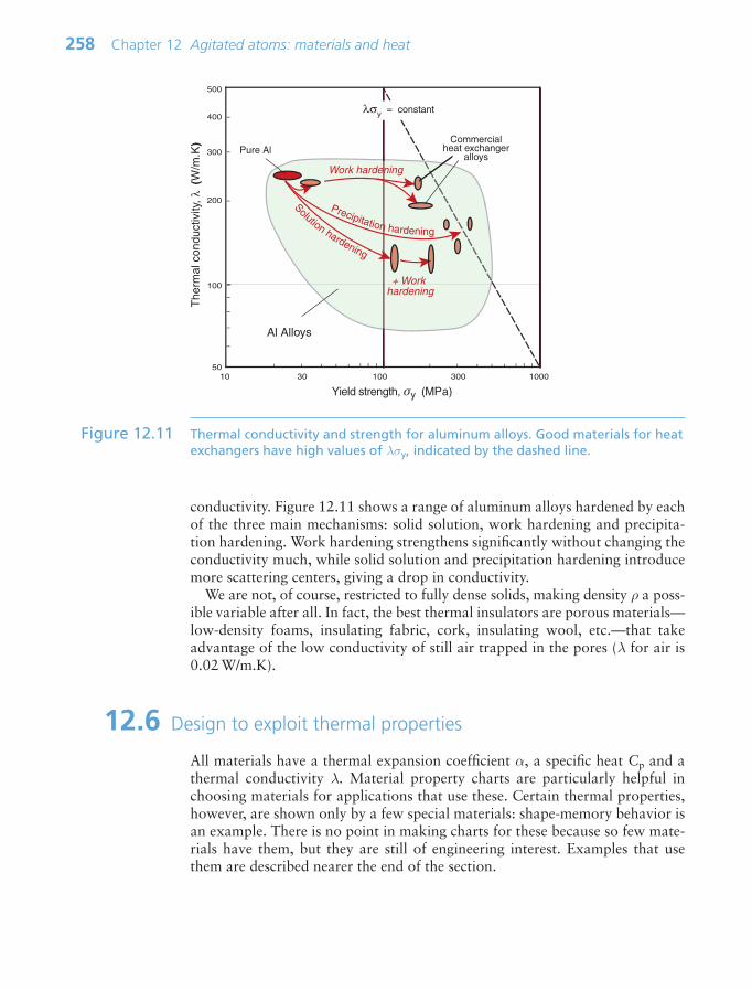
conductivity. Figure 12.11 shows a range of aluminum alloys hardened by eachof the three main mechanisms: solid solution, work hardening and precipita-tion hardening. Work hardening strengthens significantly without changing theconductivity much, while solid solution and precipitation hardening introducemore scattering centers, giving a drop in conductivity.
We are not, of course, restricted to fully dense solids, making density ρ a poss-ible variable after all. In fact, the best thermal insulators are porous materials—low-density foams, insulating fabric, cork, insulating wool, etc.—that takeadvantage of the low conductivity of still air trapped in the pores (λ for air is0.02 W/m.K).
12.6 Design to exploit thermal properties
All materials have a thermal expansion coefficient α, a specific heat Cp and athermal conductivity λ. Material property charts are particularly helpful inchoosing materials for applications that use these. Certain thermal properties,however, are shown only by a few special materials: shape-memory behavior isan example. There is no point in making charts for these because so few mate-rials have them, but they are still of engineering interest. Examples that usethem are described nearer the end of the section.
258 Chapter 12 Agitated atoms: materials and heat
10 100 1000
The
rmal
con
duct
ivity
, λ (
W/m
.K)
Al Alloys
Pure Al
100
50
500
Work hardening
Commercialheat exchanger
alloys
+ Work hardening
Yield strength, σy (MPa)
200
300
400
30 300
λσy = constant
Precipitation hardening
Solution hardening
Figure 12.11 Thermal conductivity and strength for aluminum alloys. Good materials for heatexchangers have high values of λσy, indicated by the dashed line.
Ch12-H8391.qxd 1/16/07 6:07 PM Page 258

Managing thermal stressMost structures, small or large, are made of two or more materials that areclamped, welded or otherwise bonded together. This causes problems whentemperatures change. Railway track will bend and buckle in exceptionally hotweather (steel, high α, clamped to mother earth with a much lower α).Overhead transmission lines sag for the same reason—a problem for high-speed electric trains. Bearings seize, doors jam. Thermal distortion is a particu-lar problem in equipment designed for precise measurement or registration likethat used to make masks for high-performance computer chips, causing loss ofaccuracy when temperatures change.
All of these derive from differential thermal expansion, which, if constrained(clamped in a way that stops it happening) generates thermal stress. As anexample, many technologies involve coating materials with a thin surface layerof a different material to impart wear resistance, or resistance to corrosion oroxidation. The deposition process often operates at a high temperature. Oncooling, the substrate and the surface layer contract by different amountsbecause their expansion coefficients differ and this puts the layer under stress.This residual stress calculated as follows.
Think of a thin film bonded onto a component that is much thicker than thefilm, as in Figure 12.12(a). First imagine that the layer is detached, as in Figure12.12(b). A temperature drop of ∆T causes the layer to change in length byδL1 α1L0∆T. Meanwhile, the substrate to which it was previously bonded
12.6 Design to exploit thermal properties 259
Length at temp T1 Lo (1 α1∆T )
σ
Lo (1 − α2∆T )
σ
L0 L0
Massive body with thincoating all at temperature To
Separate
Cool body to T1
Strain (α1 α2) ∆T
Stretch film Rebond
Stress E (α1 α2) ∆T
T1T1T1
To
x
(a) (b)
(c) (d) (e)
Figure 12.12 Thermal stresses in thin films arise on cooling or heating when their expansioncoefficients differ. Here that of the film is α1 and that of the substrate, a massivebody, is α2.
Ch12-H8391.qxd 1/16/07 6:07 PM Page 259
contracts by δL2 α2L0∆T. If α1 α2 the surface layer shrinks more than thesubstrate. If we want to stick the film back on the much-more-massive sub-strate, covering the same surface as before, we must stretch it by the strain
This requires a stress10 in the film of
α1 E1(α1 α2)∆T (12.11)
The stress can be large enough to crack the surface film. The pattern of cracksseen on glazed tiles arises in this way.
So if you join dissimilar materials you must expect thermal stress when theyare heated or cooled. The way to avoid it is to avoid material combinationswith very different expansion coefficients. The α–λ chart of Figure 12.4 hasexpansion α as one of its axes: benign choices are those that lie close togetheron this axis, dangerous ones are those that lie far apart.
But avoiding materials with α mismatch is not always possible. Think of join-ing glass to metal—Pyrex to stainless steel, say—a common combination in highvacuum equipment. Their expansion coefficients can be read from the α–λ chartof Figure 12.4: for Pyrex (borosilicate glass), α 4 106/K; for stainless steel,α 20 106/K: a big mismatch. Vacuum equipment has to be ‘baked out’ todesorb gases and moisture, requiring that it be heated to about 150°C, enoughfor the mismatch to crack the Pyrex. The answer is to grade the joint with oneor more materials with expansion that lies between the two: first join the Pyrexto a glass of slightly higher expansion and the stainless to a metal of lowerexpansion—the chart suggests soda glass for the first and a nickel alloy for thesecond—and then diffusion-bond these to each other, as in Figure 12.13. Thegraded joint spreads the mismatch, lowering the stress and the risk of damage.
There is an alternative, although it is not always practical. It is to put a com-pliant layer—rubber, for instance—in the joint; it is the way windows aremounted in cars. The difference in expansion is taken up by distortion in therubber, transmitting very little of the mismatch to the glass or surrounding steel.
Thermal sensing and actuationThermal expansion can be used to sense (to measure temperature) and to actu-ate (to open or close valves or electrical circuits, for instance). The direct ther-mal displacement δ αLo∆T is small; it would help to have a way to magnifyit. Figure 12.14 shows one way to do this. Two materials, deliberately chosen tohave different expansion coefficients α1 and α2, are bonded together in the form
εδ δ
α α
L L
LT1 2
01 2∆ ( )
260 Chapter 12 Agitated atoms: materials and heat
10 Strictly, E should be replaced by E/(1 ν), where ν is Poisson’s ratio, because the loadingis bi-axial.
Ch12-H8391.qxd 1/16/07 6:07 PM Page 260

of a bi-material strip, of thickness 2t, as in Figure 12.14(a). When the tempera-ture changes by ∆T (T1 To), one expands more than the other, causing thestrip to bend. The mid-thickness planes of each strip (dotted in Figure 12.14(b))differ in length by Lo (α2 α1)∆T. Simple geometry then shows that
R tR
T
1 2 1( )α α ∆
12.6 Design to exploit thermal properties 261
Radius R
Expansion coefficient α1
Expansion coefficient α2
δmax
Radius R + t
(a)Temperature To
(b)Temperature T1
δmax = (α2 − α1) ∆TL2
8 to
Displacement
L0
t
t
Figure 12.14 The thermal response of a bi-material strip when the expansion coefficients ofthe two materials differ. The configuration magnifies the thermal strain.
Stainless steel
Low α nickel alloy
High α glass
Pyrex
Figure 12.13 A graded joint. The high expansion stainless steel is bonded to a nickel alloy of lower expansion, the low expansion Pyrex (a borosilicate glass) is bonded to a glass with higher expansion, and the set are assembled to give a stepwisegraded expansion joint.
Ch12-H8391.qxd 1/16/07 6:07 PM Page 261
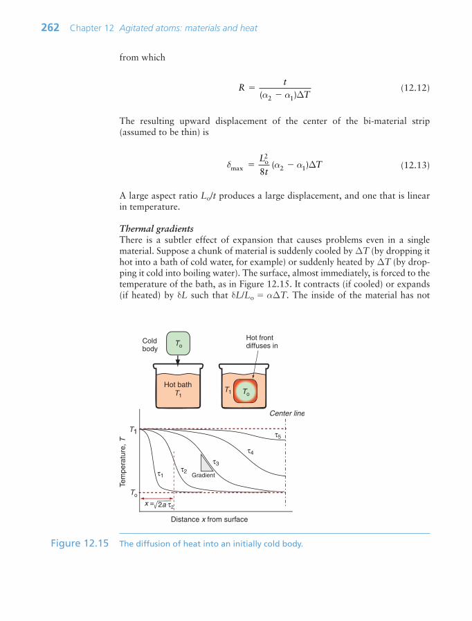
from which
(12.12)
The resulting upward displacement of the center of the bi-material strip(assumed to be thin) is
(12.13)
A large aspect ratio Lo/t produces a large displacement, and one that is linearin temperature.
Thermal gradientsThere is a subtler effect of expansion that causes problems even in a singlematerial. Suppose a chunk of material is suddenly cooled by ∆T (by dropping ithot into a bath of cold water, for example) or suddenly heated by ∆T (by drop-ping it cold into boiling water). The surface, almost immediately, is forced to thetemperature of the bath, as in Figure 12.15. It contracts (if cooled) or expands(if heated) by δL such that δL/Lo α∆T. The inside of the material has not
δ α αmaxo2
2 18
L
tT( )∆
Rt
T
( )α α2 1 ∆
262 Chapter 12 Agitated atoms: materials and heat
To
T1
Tem
pera
ture
, T
Distance x from surface
Center line
τ1τ2
τ3
τ4
τ5
Cold body
Hot bath
Hot frontdiffuses inTo
T1T1
Gradient
x = 2a τ2
To
Figure 12.15 The diffusion of heat into an initially cold body.
Ch12-H8391.qxd 1/16/07 6:07 PM Page 262
expanded yet—there has not been time for the heat to diffuse into it. That meansthere is a temperature gradient, and even though the material has just one expan-sion coefficient, there are different strains in different places. Since the surface isstuck to the interior, it is constrained, so thermal stresses appear in it just as theydid in the thin film of Figure 12.12. In brittle materials, these stresses can causefracture. The ability of a material to resist this, its thermal shock resistance, ∆Ts(units: K or °C), is the maximum sudden change of temperature to which such amaterial can be subjected without damage.
Even if the stresses do not cause failure, temperature gradients lead to distor-tion. Which properties minimize this? Figure 12.15 shows the temperature pro-file in the quenched body at successive times τ11, τ22 . . . τ55. A cooling or heatingfront propagates inwards from the surface by the process of heat diffusion dis-cussed earlier—and while it is happening there is a temperature gradient andconsequent thermal stress. If the material remains elastic, then the stresses fadeaway when the temperature is finally uniform—though the component may bythen have cracked. If the material partially yields, the stresses never go away,even when the temperature profile has smoothed out, because the surface hasyielded but the center has not. This residual stress is a major problem in metalprocessing, particularly welding, causing distortion and failure in service.
The important new variable here is time—it is this that distinguishes the con-tours in Figure 12.15. The material property that determines this time is thethermal diffusivity a that we encountered earlier:
(12.14)
with units of m2/s. The bigger the conductivity, λ, the faster the diffusivity, a,but why is ρCp on the bottom? If this quantity, the heat capacity per unit vol-ume, is large, a lot of heat has to diffuse in or out of unit volume to change thetemperature much. The more that has to diffuse, the longer it takes to do so, sothat the diffusivity a is reduced. If you solve transient heat flow problems (ofwhich this is an example), a general result emerges: it is that the characteristicdistance x (in meters) that heat diffuses in a time τ (in seconds) is
(12.15)
This is a particularly useful little formula, and although approximate (becausethe constant of proportionality, here 2, actually depends somewhat on thegeometry of the body into which the heat is diffusing), it is perfectly adequatefor first estimates of heating and cooling times.
Thermal distortion due to thermal gradients is a problem in precision equip-ment in which heat is generated by the electronics, motors, actuators or sensorsthat are necessary for its operation: different parts of the equipment are at
x a≈ 2 τ
aC
λ
ρ p
12.6 Design to exploit thermal properties 263
Ch12-H8391.qxd 1/16/07 6:07 PM Page 263

different temperatures and so expand by different amounts. The answer is tomake the equipment from materials with low expansion α (because this mini-mizes the expansion difference in a given temperature gradient) and with highconductivity λ (because this spreads the heat further, reducing the steepness ofthe gradient). It can be shown that the best choice is that of materials with highvalues of the ratio λ/α, just as our argument suggests.
The α–λ chart of Figure 12.4 guides selection for this too. The diagonal con-tours show the quantity λ/α. Materials with the most attractive values lie towardsthe bottom right. Copper, aluminum, silicon, aluminum nitride and tungsten aregood—they distort the least; stainless steel and titanium are much less good.
Conduction with strength: heat exchangersA heat exchanger transfers heat from one fluid to another while keeping the flu-ids physically separated. You find them in central heating systems, power-gen-erating plants, and cooling systems in car and marine engines. Heat istransferred most efficiently if the material separating the fluids is kept thin andif the surface area for heat conduction is large—a good solution is a tubularcoil. At least one of the fluids is under pressure, so the tubes must be strongenough to withstand it. Here there is a conflict in the design: thinner walls con-duct heat faster, thicker walls are stronger. How is this trade-off optimized bychoosing the tube material?
Consider the idealized heat exchanger made of thin-walled tubes shown inFigure 12.16. The tubes have a given radius r, a wall thickness t (which may bevaried) and must support an internal pressure of p, with a temperature differenceof ∆T between the fluids. The objective is to maximize the heat transferred perunit surface area of tube wall. The heat flow rate per unit area is given by
(12.16)qTx
Tt
λ λdd
≈∆
264 Chapter 12 Agitated atoms: materials and heat
Fluid 2
Fluid 1
tT = T1 − T2p = p1 − p2
Pressure p2, Temperature T2
Pressure p1, Temperature T1
2r
Figure 12.16 A heat exchanger. It must transmit heat yet withstand the pressure p.
Ch12-H8391.qxd 1/16/07 6:07 PM Page 264
The stress due to the internal pressure in a cylindrical thin-walled tube(Chapter 10, equation (10.7)) is
This stress must not exceed the yield strength σy of the material of which it ismade, so the minimum thickness t needed to support the pressure p is
(12.17)
Combining equations (12.16) and (12.17) to eliminate the free variable t gives
(12.18)
The best materials are therefore those with the highest values of the index λσy.They are the ones at the top right of the λ–σy chart of Figure 12.6—metals and cer-tain ceramics. Ceramics are brittle and difficult to shape into thin-walled tubes,leaving metals as the only viable choice. The chart shows that the best of these arethe alloys of copper and of aluminum. Both offer good corrosion resistance, butaluminum wins where cost and weight are to be kept low—in automotive radia-tors, for example. Commercial aluminum alloys used for this application are iden-tified in Figure 12.11. They do not offer quite the highest values of λ σy amongstthe aluminum alloys—other factors are at work here. One is the continuous expo-sure to temperature during service, which can soften the precipitation-hardenedalloys; another is that an efficient manufacturing route for thin-walled multi-chan-nel tubing is extrusion, for which high ductility is needed.
Many aluminum alloys corrode in salt water. Marine heat exchangers usecopper alloys even though they are heavier and more expensive because of theirresistance to corrosion in seawater.
Insulation: thermal wallsBefore 1940 few people had central heating or air-conditioning. Now mosthave both, and saunas and freezers and lots more. All consume power, and con-suming power is both expensive and hard on the environment (Chapter 20). Tosave on both, it pays to insulate. Consider, as an example, the oven of Figure12.17. The power lost per m2 by conduction through its wall is
(12.19)
where t is the thickness of the insulation, T0 is the temperature of the outside and Ti that of the inside. For a given wall thickness t the power consumption is
qT T
t
λ
( )i o 2W/m
qpR
λσy∆Τ
t pR
σy
σ pRt
12.6 Design to exploit thermal properties 265
Ch12-H8391.qxd 1/16/07 6:07 PM Page 265
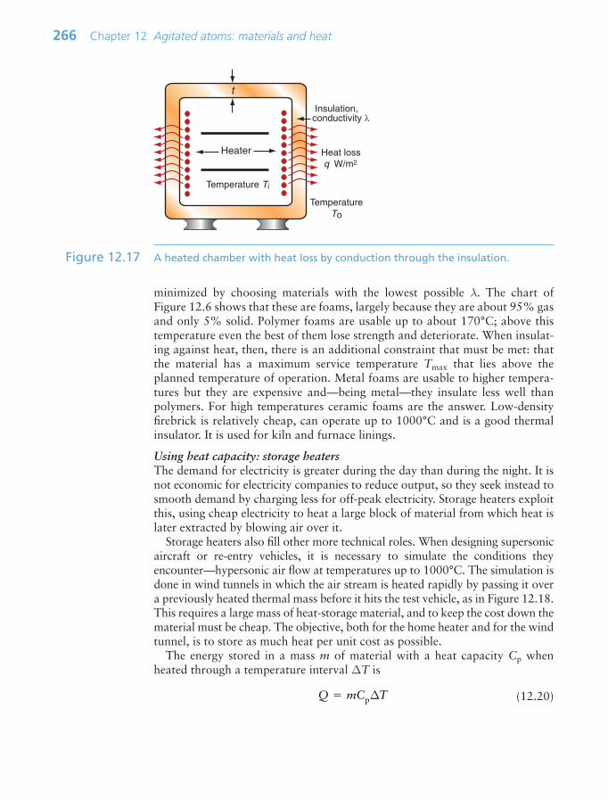
minimized by choosing materials with the lowest possible λ. The chart ofFigure 12.6 shows that these are foams, largely because they are about 95% gasand only 5% solid. Polymer foams are usable up to about 170°C; above thistemperature even the best of them lose strength and deteriorate. When insulat-ing against heat, then, there is an additional constraint that must be met: thatthe material has a maximum service temperature Tmax that lies above theplanned temperature of operation. Metal foams are usable to higher tempera-tures but they are expensive and—being metal—they insulate less well thanpolymers. For high temperatures ceramic foams are the answer. Low-densityfirebrick is relatively cheap, can operate up to 1000°C and is a good thermalinsulator. It is used for kiln and furnace linings.
Using heat capacity: storage heatersThe demand for electricity is greater during the day than during the night. It isnot economic for electricity companies to reduce output, so they seek instead tosmooth demand by charging less for off-peak electricity. Storage heaters exploitthis, using cheap electricity to heat a large block of material from which heat islater extracted by blowing air over it.
Storage heaters also fill other more technical roles. When designing supersonicaircraft or re-entry vehicles, it is necessary to simulate the conditions theyencounter—hypersonic air flow at temperatures up to 1000°C. The simulation isdone in wind tunnels in which the air stream is heated rapidly by passing it overa previously heated thermal mass before it hits the test vehicle, as in Figure 12.18.This requires a large mass of heat-storage material, and to keep the cost down thematerial must be cheap. The objective, both for the home heater and for the windtunnel, is to store as much heat per unit cost as possible.
The energy stored in a mass m of material with a heat capacity Cp whenheated through a temperature interval ∆T is
(12.20)Q mC T p∆
266 Chapter 12 Agitated atoms: materials and heat
Temperature Ti
Temperature To
Insulation,conductivity λ
Heater
t
Heat loss q W/m2
Figure 12.17 A heated chamber with heat loss by conduction through the insulation.
Ch12-H8391.qxd 1/16/07 6:07 PM Page 266

The cost of mass m of material with a cost per kg of Cm is
Thus, the heat stored per unit material cost is
(12.21)
The best choice of material is simply that with the largest heat capacity, Cp, andlowest price, Cm. There is one other obvious constraint: the material must beable to tolerate the temperature to which it will be heated—say, Tmax 150°Cfor the home heater, Tmax 1000°C for the air tunnel. It is hard to do thisselection with the charts provided here, but easy to do it with the CES software:apply the limit on Tmax then use the index
to isolate the cheapest candidates. You will find that the best choice for thehome heater is concrete (cast to a shape that provides some air channels). Forthe wind tunnel, in which temperatures are much higher, the best choice is arefractory brick with air channels for rapid heat extraction.
Using phase change: thermal buffersWhen materials vaporize, or melt, or change their crystal structure while remain-ing solid (all of which are known as ‘phase changes’), many things happen, and
MC
C
p
m
QC
C
C
p
m
C mC m
12.6 Design to exploit thermal properties 267
Testvehicle
Heat-storing material: high Cp, adequate Tmax
Fan
Hotair
Coldair
Figure 12.18 A wind tunnel with storage heating. The thermal mass is pre-heated, giving upits heat to the air blast when the fan is activated.
Ch12-H8391.qxd 1/16/07 6:07 PM Page 267
they can be useful. They change in volume. If solid, they may change in shape.And they absorb or release heat, the latent heat L (J/kg) of the phase change,without changing temperature.
Suppose you want to keep something at a fixed temperature without exter-nal power. Perfect insulation is not just impractical, it is impossible. But—ifkeeping things warm is the problem—the answer is to surround them by a liq-uid that solidifies at the temperature that you want to maintain. As it solidifiesit releases its latent heat of fusion, holding the temperature precisely at its solid-ification temperature (i.e. its melting point) until all the liquid is solid—it is theprinciple on which some food warmers and ‘back-woods’ hand warmers work.The reverse is also practical: using latent heat of melting to keep things cool.For this, choose a solid that melts, absorbing latent heat, at the temperatureyou want to maintain—‘cool bag’ inserts for holiday travel work in this way. Inboth cases, change of phase is used as a thermal buffer.
Shape-memory and super-elastic materialsAlmost all materials expand on heating and shrink on cooling. Some few havea different response, one that comes from a solid-state phase change. Shape-memory materials are alloys based on titanium or nickel that can, while stillsolid, exist in two different crystal configurations with different shapes, calledallotropes. If you bend the material it progressively changes structure from theone allotrope to the other, allowing enormous distortion. Shape-memory alloyshave a critical temperature. If below this critical temperature, the distorted mate-rial just stays in its new shape. Warm it up and, at its critical temperature, thestructure reverts to the original allotrope and the sample springs back to its orig-inal shape. This has obvious application in fire alarms, sprinkler systems andother temperature-controlled safety systems, and they are used for all of these.
But what if room temperature is already above this critical temperature?Then the material does not sit waiting for heat, but springs back to its originalshape as soon as released, just as if it were elastic. The difference is that thephase change allowed distortions which are larger, by a factor of 100 or more,than straightforward elasticity without the phase change. The material is super-elastic. It is just what is needed for eyeglass frames that get sat on and other-wise mistreated, or springs that must allow very large displacements atconstant restoring force—and these, indeed, are the main applications for thesematerials.
12.7 Summary and conclusions
All materials have:
• A specific heat, Cp: the amount of energy it takes to heat unit mass by unittemperature.
• A thermal expansion, α: the change in its dimensions with change of temperature.
268 Chapter 12 Agitated atoms: materials and heat
Ch12-H8391.qxd 1/16/07 6:07 PM Page 268

• A thermal conductivity λ and thermal diffusivity a: the former characterizinghow fast heat is transmitted through the solid, the latter how long it takes forthe temperature, once perturbed, to settle back to a steady pattern.
• Characteristic temperatures of its changes of phase or behavior: for a crys-talline solid, its melting point Tm, and for non-crystalline solids, a glass transi-tion temperature Tg; for design in all materials, an empirical temperature maybe defined, the maximum service temperature Tmax, above which, for reasonsof creep or degradation, continuous use is impractical.
• Latent heats of melting and of vaporization: the energy absorbed or releasedat constant temperature when the solid melts or evaporates.
These properties can be displayed as material property charts—examples ofwhich are utilized in this chapter. The charts illustrate the great range of thermalproperties and the ways they are related. To explain these we need an under-standing of the underlying physics. The key concepts are that thermal energy isatomic-level vibration, that increasing the amplitude of this vibration causesexpansion, and that the vibrations propagate as phonons, giving conduction. Inmetals the free electrons—the ones responsible for electrical conduction—alsotransport heat, and they do so more effectively than phonons, giving metals theirhigh thermal conductivities. Thermal properties are manipulated by interferingwith these processes: alloying to scatter phonons and electrons; foaming todilute the solid with low-conductivity, low-specific-heat gases.
The thermal response can be a problem in design—thermal stress, forinstance, causes cracking. It can also be useful—thermal distortion can be usedfor actuation or sensing. It is the specific heat that makes an oven take 15 min-utes to warm up, but it also stores heat in a way that can be recovered ondemand. Good thermal conduction is not what you want in a coffee cup, butwhen it cools the engine of your car or the chip in your computer it is a big help.
This chapter has been about the thermal properties of materials. Heat, as wehave said, also changes other properties, mechanical and electrical. We lookmore deeply into that in Chapter 13.
12.8 Further reading
Cottrell, A.H. (1964) The Mechanical Properties of Matter, Wiley, London, UK. Libraryof Congress number 64-14262. (The best introduction to the physical understandingof the properties of materials, now out of print but worth searching for.)
Hollman, J.P. (1981) Heat Transfer, 5th edition, McGraw-Hill, New York, USA. ISBN0-07-029618-9. (A good starting point: an elementary introduction to the principlesof heat transfer.)
Tabor, D. (1969) Gases, Liquids and Solids, Penguin Books, Harmondsworth, UK.ISBN 14-080052-2. (A concise introduction to the links between inter-atomic forcesand the bulk properties of materials.)
12.8 Further reading 269
Ch12-H8391.qxd 1/16/07 6:07 PM Page 269

270 Chapter 12 Agitated atoms: materials and heat
12.9 Exercises
Exercise E12.1 Define specific heat. What are its units? How would you calculate the spe-cific heat per unit volume from the specific heat per unit mass? If youwanted to select a material for a compact heat storing device, which of thetwo would you use as a criterion of choice?
Exercise E12.2 What two metals would you choose from the λ–a chart of Figure 12.5 tomaximize the thermal displacement of a bi-metallic strip actuator? If thebimetallic strip has thickness 2 mm and average thermal diffusivity a of5 105/°C, how long will it take to respond when the temperature sud-denly changes?
Exercise E12.3 A new alloy has a density of 7380 kg/m3. Its specific heat has not yet beenmeasured. How would you make an approximate estimate of its value inthe normal units of J/kg.K? What value would you then report?
Exercise E12.4 The same new alloy of the last exercise has a melting point of 1540 K. Its ther-mal expansion coefficient has not yet been measured. How would you makean approximate estimate of its value? What value would you then report?
Exercise E12.5 Interior wall insulation should insulate well, meaning low thermal conduc-tivity, λ, but require as little heat as possible to warm up when the centralheating system is turned on (if the wall absorbs heat the room stays cold).Use the λ–a chart of Figure 12.5 to find the materials that do this best (thecontours will help).
Exercise E12.6 You notice that the ceramic coffee mugs in the office get too hot to hold about10 seconds after pouring in the hot coffee. The wall thickness of the cup is 2mm.
(a) What, approximately, is the thermal diffusivity of the ceramic of the mug?(b) Given that the volume specific heat of solids, ρCp, is more or less constant
at 2 106J/m3 K, what approximately is the thermal conductivity ofthe cup material?
(c) If the cup were made of a metal with a thermal diffusivity of2 105m2/s, how long could you hold it?
Exercise E12.7 A structural material is sought for a low-temperature device for use at 20°Cthat requires high strength but low thermal conductivity. Use the λ–σy chartof Figure 12.6 to suggest two promising candidates (reject ceramics on thegrounds that they are too brittle for structural use in this application).
Exercise E12.8 A material is needed for a small, super-efficient pressurized heat exchanger.The text explained that the index for this application is M λσy. Plot con-tours of this index onto a copy of the λ–σy chart of Figure 12.6 and hencefind the two classes of materials that maximize M.
Ch12-H8391.qxd 1/16/07 6:07 PM Page 270
12.10 Exploring design with CES 271
12.10 Exploring design with CES (use Level 2, Materials, for all selections)
Exercise E12.9 Use the ‘Search’ facility of CES to find materials for:
(a) Thermal insulation.(b) Heat exchangers.
Exercise E12.10 The analysis of storage heaters formulated the design constraints for theheat-storage material, which can be in the form of a particle bed or a solidblock with channels to pass the air to be heated. Use the selector to find thebest materials. Here is a summary of the design requirements. List the topsix candidates in ranked order.
Exercise E12.11 The requirements for a material for an automobile radiator, described inthe text, are summarized in the table. Use CES to find appropriate materi-als to make them. List the top four candidates in ranked order.
Exercise E12.12 A structural material is sought for a low-temperature device for use at20°C that requires high tensile strength σts but low thermal conductivityλ. For reasons of damage tolerance the fracture toughness K1c must begreater than 15 MPa.m1/2. Apply the constraint on K1c using a ‘Limit’stage, then make a chart with σts on the x-axis and λ on the y-axis, andobserve which materials best meet the requirements. Which are they?
Function • Automobile heat exchanger
Constraints • Elongation 10%• Maximum use temperature 180°C• Price $5/kg• Durability in fresh water very good
Objective • Maximize thermal conductivity yieldstrength, λσy
• Wall thickness, t
Free variables • Choice of material
Function • Storage heater
Constraints • Maximum service temperature 150°C• Non-flammable (a durability rating)
Objective • Maximize specific heat/material cost, Cp/Cm
Free variables • Choice of material
Ch12-H8391.qxd 1/16/07 6:07 PM Page 271
272 Chapter 12 Agitated atoms: materials and heat
Exercise E12.13 Interior wall insulation should insulate well, meaning low thermal conduc-tivity, λ, but require as little heat as possible to warm up to the desired roomtemperature when the central heating system is turned on—that means lowspecific heat. The thickness of the insulation is almost always limited by thecavity space between the inner and outer wall, so it is the specific heat per unitvolume, not per unit mass, that is important here. To be viable the materialmust have enough stiffness and strength to support its own weight and beeasy to install—take that to mean a modulus E 0.01 GPa and a strengthσy 0.1 MPa. Make a selection based on this information. List the materialsyou find that best meet the design requirements.
Exercise E12.14 Here is the gist of an email one of the authors received as this chapter wasbeing written. ‘We manufacture wood-burning stoves and fireplaces thatare distributed all over Europe. We want to select the best materials forour various products. The important characteristics for us are: specificheat, thermal conductivity, density . . . and price, of course. What canyour CES software suggest?’
Form your judgement about why these properties matter to them. Rankthem, deciding which you would see as constraints and which as the objec-tive. Consider whether there are perhaps other properties they have neg-lected. Then—given your starting assumptions of just how these stoves areused—use CES to make a selection. Justify your choice.
There is no ‘right’ answer to this question—it depends on the assump-tions you make. The essence is in the last sentence of the last paragraph:justify your choice.
12.11 Exploring the science with CES Elements
Exercise E12.15 The text says that materials expand about 2% between 0 K and their melt-ing point. Use CES Elements to explore the truth of this by making a barchart of the expansion at the melting point, αTm/106 (the 106 is to correctfor the units of α used in the database).
Exercise E12.16 When a solid vaporizes, the bonds between its atoms are broken. Youmight then expect that latent heat of vaporization, Lv, should be nearly thesame as the cohesive energy, Hc, since it is the basic measure of the strengthof the bonding. Plot one against the other, using CES Elements. How closeare they?
Ch12-H8391.qxd 1/16/07 6:07 PM Page 272

12.11 Exploring the science with CES Elements 273
Exercise E12.17 When a solid melts, some of the bonds between its atoms are broken, butnot all—liquids still have a bulk modulus, for example. You might thenexpect that the latent heat of melting, Lm, should be less than the cohesiveenergy, Hc, since it is the basic measure of the strength of the bonding. Plotone against the other, using CES Elements (Lm is called the heat of fusion inthe database). By what factor is Lm less than Hc? What does this tell youabout cohesion in the liquid?
Exercise E12.18 The latent heat of melting (heat of fusion), Lm, of a material is said to beabout equal to the heat required to heat it from absolute zero to its melt-ing point, CpTm, where Cp is the specific heat and Tm is the absolute melt-ing point. Make a chart with Lm on one axis and Cp Tm on the other. Tomake the comparison right we have to change the units of Lm in makingthe chart to J/kg instead of kJ/mol. To do this multiply Lm by
using the ‘Advanced’ facility when defining axes in CES. Is the statement true?
Exercise E12.19 The claim was made in the text that the modulus E is roughly proportionalto the absolute melting point Tm. If you use CES Elements to explore this cor-relation you will find that it is not, in fact, very good (try it). That is becauseTm and E are measured in different units and, from a physical point of view,the comparison is meaningless. To make a proper comparison, we use insteadkBTm and EΩ, where kB is Boltzmann’s (1.38 1023J/K) constant andΩm3/atom is the atomic volume. These two quantities are both energies, thefirst proportional to the thermal energy per atom at the melting point and thesecond proportional to the work to elastically stretch an atomic bond. Itmakes better sense, from a physical standpoint, to compare these.
Make a chart for the elements with kBTm on the x-axis and EΩ on the y-axis to explore how good this correlation is. Correlations like these (if good)that apply right across the Periodic Table provide powerful tools for check-ing data, and for predicting one property (say, E) if the other (here, Tm ) isknown. Formulate an equation relating the two energies that could be usedfor these purposes.
Exercise E12.20 Above the Debye temperature, the specific heat is predicted to be 3R,where R is in units of kJ/kmol.K. Make a plot for the elements with Debyetemperature on the x-axis and specific heat in these units on the y-axis toexplore this. You need to insert a conversion factor because of the units.Here it is, expressed in the units contained in the database:
Specific heat in kJ/kmol.K Specific heat in J/kg.K Atomic weight in kg/kmol /1000.
10Atomic weight in kg/kmol
6
Ch12-H8391.qxd 1/16/07 6:07 PM Page 273

Form this quantity, dividing the result by R 8.314 kJ/kmol.K, andplot it against the Debye temperature. The result should be 3 except formaterials with high Debye temperatures. Is it? Fit a curve by eye to thedata. At roughly what temperature does the drop-off first begin?
Exercise E12.21 Explore the mean free path of phonons m in the elements using equation(12.10) of the text. Inverting it gives
in which the speed of sound co E/ρ. Use the ‘Advanced’ facility whendefining the axes in CES to make a bar chart of m for the elements. Whichmaterials have the longest values? Which have the shortest?
mp o
3λ
ρC c
274 Chapter 12 Agitated atoms: materials and heat
Ch12-H8391.qxd 1/16/07 6:07 PM Page 274

Chapter 13Running hot: using materials
at high temperatures
Chapter contents
13.1 Introduction and synopsis 27613.2 The temperature dependence of
material properties 27613.3 Charts for creep behavior 28113.4 The science: diffusion and creep 28413.5 Materials to resist creep 29313.6 Design to cope with creep 29613.7 Summary and conclusions 30413.8 Further reading 30513.9 Exercises 30513.10 Exploring design with CES 30813.11 Exploring the science with
CES Elements 308
Shuttle flame. (Image courtesy of C. MichaelHoloway, NASA Langley, USA.)
Ch13-H8391.qxd 1/16/07 1:42 PM Page 275

276 Chapter 13 Running hot: using materials at high temperatures
13.1 Introduction and synopsis
Material properties change with temperature. Some do so in a simple linear way,easy to allow for in design: the density, the modulus and the electrical conduc-tivity are examples. But others, particularly the yield strength and the rates ofoxidation and corrosion, change in more sudden ways that, if not allowed for,can lead to disaster.
This chapter explores the ways in which properties change with temperatureand design methods to deal with the changes. To do this we must first understanddiffusion—the intermixing of atoms in solids—and the ways it allows creep andcreep fracture. This understanding lies behind procedures for high-temperaturedesign with metals and ceramics. Polymers are a little more complicated in theirbehavior, but semi-empirical methods allow safe design with these too.
13.2 The temperature dependence of material properties
Maximum and minimum service temperaturesFirst, the simplest measure of tolerance to temperature: the maximum and mini-mum service temperatures, Tmax and Tmin. The former tells us the highest temper-ature at which the material can reasonably be used without oxidation, chemicalchange or excessive deflection or ‘creep’ becoming a problem (the continuoususe temperature, or CUT, is a similar measure). The latter is the temperaturebelow which the material becomes brittle or otherwise unsafe to use. These areempirical, with no universally accepted definitions. The minimum service tem-perature for carbon steels is the ductile-to-brittle-transition temperature—atemperature below which the fracture toughness falls steeply. For elastomers itis about 0.8 Tg, where Tg is the glass temperature; below Tg they cease to berubbery and become hard and brittle.
Linear and nonlinear temperature dependenceSome properties depend on temperature T in a linear way, meaning that
(13.1)
where P is the value of the property, Po its low-temperature value and β is aconstant. Figure 13.1 shows four examples: density, modulus, refractive indexand—for metals—electrical resistivity. Thus, the density ρ and refractive indexn decrease by about 6% on heating from cold to the melting point Tm(β 0.06), the modulus E falls by a factor of 2 (β 0.5), and the resistiv-ity R increases by a factor of about 7 (β 6). These changes cannot be neg-lected, but are easily accommodated by using the value of the property at thetemperature of the design.
P PTTo≈
⎛
⎝⎜⎜⎜⎜
⎞
⎠⎟⎟⎟⎟⎟
1m
β
Ch13-H8391.qxd 1/16/07 1:42 PM Page 276
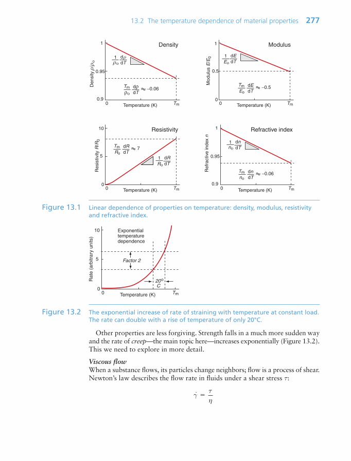
13.2 The temperature dependence of material properties 277
Other properties are less forgiving. Strength falls in a much more sudden wayand the rate of creep—the main topic here—increases exponentially (Figure 13.2).This we need to explore in more detail.
Viscous flowWhen a substance flows, its particles change neighbors; flow is a process of shear.Newton’s law describes the flow rate in fluids under a shear stress τ:
γη
.
τ
dρdT
Tmρο
−0.06
Temperature (K)0 Tm
d ρdT
Den
sity
ρ/ρ
ο
1
0.9
0.95
ρο1
Temperature (K)0 Tm
10
0
5
Res
istiv
ity R
/R0
dRdT
TmRo
7
dRdTRο
1
Temperature (K)0 Tm0
0.5
dEdT
Mod
ulus
E/E
0
dEdT
TmEo
−0.5
Eο1
1
dndT
Tmnο
−0.06
Temperature (K)0 Tm
dndT
Ref
ract
ive
inde
x n
1
0.9
0.95
nο1
Density Modulus
Resistivity Refractive index
Figure 13.1 Linear dependence of properties on temperature: density, modulus, resistivityand refractive index.
Temperature (K)0 Tm
10
0
5
Rat
e (a
rbitr
ary
units
)
Exponential temperature dependence
Factor 2
20o C
Figure 13.2 The exponential increase of rate of straining with temperature at constant load.The rate can double with a rise of temperature of only 20°C.
Ch13-H8391.qxd 1/16/07 1:42 PM Page 277
where γ. is the shear rate and η the viscosity. This is a linear law, like Hooke’slaw, with the modulus replaced by the viscosity and the strain by strain rate (unitss1). Viscous flow occurs at constant volume (Poisson’s ratio 0.5) and thismeans that problems of viscous flow can be solved by taking the solution forelastic deformation and replacing the strain ε by the strain rate
.ε and, using
equation (4.10), Young’s modulus E by 3η. Thus, the rate at which a rod of avery viscous fluid, like tar, extends when pulled in tension is
(13.2)
The factor 1/3 appears because of the conversion from shear to normal stressand strain.
CreepAt room temperature, most metals and ceramics deform in a way that dependson stress but not on time. As the temperature is raised, loads that are too smallto give permanent deformation at room temperature cause materials to creep: toundergo slow, continuous deformation with time, ending in fracture. It is usualto refer to the time-independent behavior as ‘low-temperature’ response, and thetime-dependent flow as ‘high-temperature’ response. But what, in this context,is ‘low’ and what is ‘high’? The melting point of tungsten, used for lamp filaments,is over 3000°C. Room temperature, for tungsten, is a very low temperature.The filament temperature in a tungsten lamp is about 2000°C. This, for tungsten,is a high temperature: the filament slowly sags over time under its own weightuntil the turns of the coil touch and the lamp burns out.
To design against creep we need to know how the strain rate ε or time to failuretf depends on the stress σ and temperature T to which it is exposed. That requirescreep testing.
Creep testing and creep curvesCreep is measured in the way shown in Figure 13.3. A specimen is loadedin tension or compression, usually at constant load, inside a furnace which ismaintained at a constant temperature, T. The extension is measured as a func-tion of time. Metals, polymers and ceramics all have creep curves with the gen-eral shape shown in the figure.
The initial elastic and the primary creep strains occur quickly and can be treatedin much the way that elastic deflection is allowed for in a structure. Thereafter,the strain increases steadily with time in what is called the secondary creepor the steady-state creep regime. Plotting the log of the steady-state creep rate, εss, against the log of the stress, σ, at constant T, as in Figure 13.4(a),shows that
(13.3)ε ss B nσ
ε ση3
278 Chapter 13 Running hot: using materials at high temperatures
Ch13-H8391.qxd 1/16/07 1:42 PM Page 278

where n, the creep exponent, usually lies between 3 and 8 and for that reasonthis behavior is called power-law creep. At low σ there is a tail with slope n 1(the part of the curve labeled ‘Diffusional flow’ in Figure 13.4(a)). By plotting thenatural logarithm (ln) of ε.ss against the reciprocal of the absolute temperature(1/T) at constant stress, as in Figure 13.4(b), we find that:
(13.4)
Here R–
is the gas constant (8.31 J/mol/K) and Qc is called the activationenergy for creep, with units of J/mol. The creep rate ε.ss increases exponentially
ε sscexpC
Q
RT
⎛
⎝⎜⎜⎜⎜
⎞
⎠⎟⎟⎟⎟
13.2 The temperature dependence of material properties 279
Time t (s)
Str
ain
ε
FAo
L
1 104 106 108102
0.1
0.05
0
0.15
Initial elastic strain
Primary strainTime to
fracture, tf
Steady-state creep
Fracture
εss
Tertiarycreep
Figure 13.3 Creep testing and the creep curve, showing how strain ε increases with time tup to the fracture time tf.
Reciprocal temperature, 1/T (1/K)Log stress, σ
Ln ε. ss
Log
ε. ss
Slope - Qc
R
Power-lawcreep
Diffusionalflow
Slope n = 1
Slope n = 3 to 8
Stress dependence
Temperature dependence
(a) (b)
Figure 13.4 The stress and temperature dependence of the creep rate.
Ch13-H8391.qxd 1/16/07 1:42 PM Page 279
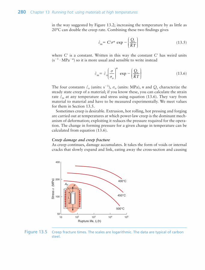
in the way suggested by Figure 13.2; increasing the temperature by as little as20°C can double the creep rate. Combining these two findings gives
(13.5)
where C is a constant. Written in this way the constant C has weird units(s1 MPan) so it is more usual and sensible to write instead
(13.6)
The four constants ε.o (units: s1), σo (units: MPa), n and Qc characterize thesteady state creep of a material; if you know these, you can calculate the strainrate ε.ss at any temperature and stress using equation (13.6). They vary frommaterial to material and have to be measured experimentally. We meet valuesfor them in Section 13.5.
Sometimes creep is desirable. Extrusion, hot rolling, hot pressing and forgingare carried out at temperatures at which power-law creep is the dominant mech-anism of deformation; exploiting it reduces the pressure required for the opera-tion. The change in forming pressure for a given change in temperature can becalculated from equation (13.6).
Creep damage and creep fractureAs creep continues, damage accumulates. It takes the form of voids or internalcracks that slowly expand and link, eating away the cross-section and causing
ε ε sscexpo
o
nQ
RTσσ
⎛
⎝⎜⎜⎜⎜
⎞
⎠⎟⎟⎟⎟⎟
⎛
⎝⎜⎜⎜⎜
⎞
⎠⎟⎟⎟⎟⎟
ε sscexpC
Q
RTnσ
⎛
⎝⎜⎜⎜⎜
⎞
⎠⎟⎟⎟⎟
280 Chapter 13 Running hot: using materials at high temperatures
Rupture life, tf (h)
Str
ess
σ (M
Pa)
FAo
L
10 103 104 105102
200
100
50
400
400°C
450°C
500°C
Figure 13.5 Creep fracture times. The scales are logarithmic. The data are typical of carbonsteel.
Ch13-H8391.qxd 1/16/07 1:42 PM Page 280

the stress to rise. This makes the creep rate accelerate as shown in the tertiarystage of the creep curve of Figure 13.3. Since ε. σn with n 5, the creep rategoes up even faster than the stress: an increase of stress of 10% gives an increasein creep rate of 60%.
Times to failure, tf, are normally presented as creep–rupture diagrams(Figure 13.5). Their application is obvious: if you know the stress and tempera-ture you can read off the life. If instead you wish to design for a certain life at acertain temperature, you can read off the design stress. Experiments show that
(13.7)
which is called the Monkman–Grant law. The Monkman–Grant constant, C, istypically 0.05–0.3. Knowing it, the creep life (meaning tf) can be estimatedfrom equation (13.6).
13.3 Charts for creep behavior
Melting pointFigure 13.6 shows melting points for metals, ceramics and polymers. Mostmetals and ceramics have high melting points and, because of this, they start tocreep only at temperatures well above room temperature. Lead, however, has amelting point of 327°C (600 K), so room temperature is almost half its absolute
ε ss ft C
13.3 Charts for creep behavior 281
Mel
ting
poin
t (°C
)
0
500
1000
1500
2000
2500
3000
3500
Ceramics PolymersMetals
Tungsten
Lead
Tungsten carbide
Alumina
Silicon nitrideZirconia
Concrete
Granite
Titanium alloys
C-steel
Nickel alloysStainless steel
Copper alloys
Aluminum alloys
Cast iron
Magnesium alloysZinc alloys
Silicon nitride
Silicon
BrickCement
Marble
PEEK
PTFE
PET Acetal PE PU
PPNylon
Figure 13.6 Melting points of ceramics, metals and polymers.
Ch13-H8391.qxd 1/16/07 1:42 PM Page 281
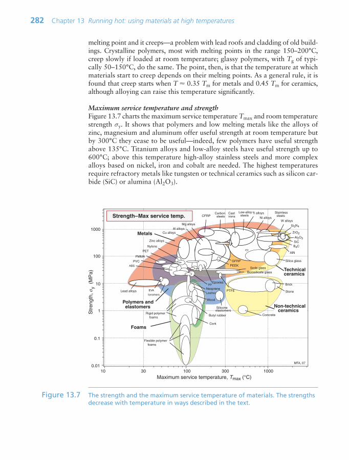
melting point and it creeps—a problem with lead roofs and cladding of old build-ings. Crystalline polymers, most with melting points in the range 150–200°C,creep slowly if loaded at room temperature; glassy polymers, with Tg of typi-cally 50–150°C, do the same. The point, then, is that the temperature at whichmaterials start to creep depends on their melting points. As a general rule, it isfound that creep starts when T 0.35 Tm for metals and 0.45 Tm for ceramics,although alloying can raise this temperature significantly.
Maximum service temperature and strengthFigure 13.7 charts the maximum service temperature Tmax and room temperaturestrength σy. It shows that polymers and low melting metals like the alloys ofzinc, magnesium and aluminum offer useful strength at room temperature butby 300°C they cease to be useful—indeed, few polymers have useful strengthabove 135°C. Titanium alloys and low-alloy steels have useful strength up to600°C; above this temperature high-alloy stainless steels and more complexalloys based on nickel, iron and cobalt are needed. The highest temperaturesrequire refractory metals like tungsten or technical ceramics such as silicon car-bide (SiC) or alumina (Al2O3).
282 Chapter 13 Running hot: using materials at high temperatures
Maximum service temperature, Tmax (°C)
Str
engt
h, σ
y (
MP
a)
0.01
0.1
1
10
100
1000
10 100 300 100030
Foams
Polymers and elastomers
Metals
Technicalceramics
Lead alloys
W alloys
Stainless steels
Ti alloys
Mg alloys
CFRP
GFRP
Al alloys
Cast irons
Cu alloys
Zinc alloys
PMMA
Epoxies
PET
Cork
Wood
Silicone elastomers
Concrete
AlN
Al2O3SiC
Si3N4
Strength–Max service temp.
Rigid polymer foams
Flexible polymer foams
ABS
Butyl rubber
EVA NeopreneLeather
Ionomers
PP
Soda glass
Silica glass
Non-technical ceramics
Brick
MFA, 07
Carbon steels Ni alloys
Low-alloy steels
B4C
Stone
Borosilicate glass
PTFE
PEEK
Nylons
PVC
ZrO2
Figure 13.7 The strength and the maximum service temperature of materials. The strengthsdecrease with temperature in ways described in the text.
Ch13-H8391.qxd 1/16/07 1:42 PM Page 282
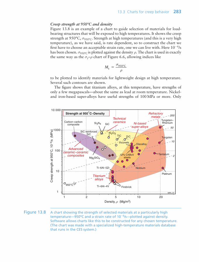
Creep strength at 950°C and densityFigure 13.8 is an example of a chart to guide selection of materials for load-bearing structures that will be exposed to high temperatures. It shows the creepstrength at 950°C, σ950°C. Strength at high temperatures (and this is a very hightemperature), as we have said, is rate dependent, so to construct the chart wefirst have to choose an acceptable strain rate, one we can live with. Here 106/shas been chosen. σ950°C is plotted against the density ρ. The chart is used in exactlythe same way as the σy–ρ chart of Figure 6.6, allowing indices like
to be plotted to identify materials for lightweight design at high temperature.Several such contours are shown.
The figure shows that titanium alloys, at this temperature, have strengths ofonly a few megapascals—about the same as lead at room temperature. Nickel-and iron-based super-alloys have useful strengths of 100 MPa or more. Only
Mt950 C σρ
13.3 Charts for creep behavior 283
Density, ρ (Mg/m3)
Cre
ep s
treng
th a
t 950
°C, 1
0−6/s
(M
Pa)
1 2 10 20
1
10
100
1000
10 000
σ950°C/ρ
Carbon–carboncomposite SiCSi3N4
Mg2SiO4
FirebrickTi–6Al–4V
Ti–6Al–5Zr Niobium
Platinum
Tungsten
Tantalum
Tungsten–Rhenium
Al2O3TiC ZrC
SiC reinforcedSiC
Strength at 950°C–Density
MFA, 07
Titaniumalloys
Refractorymetals
Ni-basedsuper-alloys
Technicalceramics
Advancedceramic–ceramic
composites 12% CrMoV steels
DiscalloyInconels
2
10
200
50
5
Figure 13.8 A chart showing the strength of selected materials at a particularly hightemperature—950ºC and a strain rate of 106/s—plotted against density.Software allows charts like this to be constructed for any chosen temperature.(The chart was made with a specialized high-temperature materials databasethat runs in the CES system.)
Ch13-H8391.qxd 1/16/07 1:42 PM Page 283

refractory metals like alloys of tungsten, technical ceramics like SiC and advanced(and very expensive) ceramic–ceramic composites offer high strength.
At room temperature we need only one strength–density chart. For high temper-ature design we need one that is constructed for the temperature and acceptablestrain rate or life required by the design. It is here that computer-aided methodsbecome particularly valuable, because they allow charts like Figure 13.8 to beconstructed and manipulated for any desired set of operating conditions quicklyand efficiently.
13.4 The science: diffusion and creep
Viscous flow and creep require the relative motion of atoms. How does thishappen, and what is its rate? Think first of the unit step—one atom changingits position relative to those around it by what is called diffusion.
DiffusionDiffusion is the spontaneous intermixing of atoms over time. In gases and liq-uids intermixing is familiar—the dispersion of smoke in still air, the dispersionof an ink drop in water—and understood as the random motion of the atomsor molecules (Brownian motion). But in crystalline solids atoms are confined tolattice sites—how then are they going to mix? In practice they do. If atoms oftype A are plated onto a block of atoms of type B and the A–B couple is heated,the atoms interdiffuse at a rate described by Fick’s law:1
(13.8)
Here J is the atom flux (the number of atoms of type A diffusing across unitarea of surface per second), D is the diffusion coefficient and dc/dx is the gra-dient in concentration c of A atoms in the x direction.
Heat, as we have said, is atoms in motion. In a solid they vibrate about theirmean position with a frequency ν (about 1013 per second) with an averageenergy, kinetic plus potential, of kBT in each mode of vibration, where kB isBoltzmann’s constant (1.38 1023 J/atom K). This is the average, but at anyinstant some atoms have less, some more. Statistical mechanics gives the distri-bution of energies. The Maxwell–Boltzmann equation describes the probabilityp that a given atom has an energy greater than a value q joules:
(13.9)pq
k T exp
B
⎛
⎝⎜⎜⎜⎜
⎞
⎠⎟⎟⎟⎟⎟
J Dcx
dd
284 Chapter 13 Running hot: using materials at high temperatures
1 Adolph Eugen Fick (1829–1901), German physicist, physiologist and inventor of the con-tact lens. He formulated the law that describes the passage of gas through a membrane,but which also describes the heat-activated mixing of atoms in solids.
Ch13-H8391.qxd 1/16/07 1:42 PM Page 284
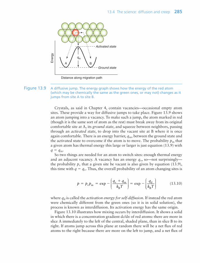
Crystals, as said in Chapter 4, contain vacancies—occasional empty atomsites. These provide a way for diffusive jumps to take place. Figure 13.9 showsan atom jumping into a vacancy. To make such a jump, the atom marked in red(though it is the same sort of atom as the rest) must break away from its originalcomfortable site at A, its ground state, and squeeze between neighbors, passingthrough an activated state, to drop into the vacant site at B where it is onceagain comfortable. There is an energy barrier, qm, between the ground state andthe activated state to overcome if the atom is to move. The probability pm thata given atom has thermal energy this large or larger is just equation (13.9) withq qm.
So two things are needed for an atom to switch sites: enough thermal energyand an adjacent vacancy. A vacancy has an energy qv, so—not surprisingly—the probability pv that a given site be vacant is also given by equation (13.9),this time with q qv. Thus, the overall probability of an atom changing sites is
(13.10)
where qd is called the activation energy for self-diffusion. If instead the red atomwere chemically different from the green ones (so it is in solid solution), theprocess is known as interdiffusion. Its activation energy has the same origin.
Figure 13.10 illustrates how mixing occurs by interdiffusion. It shows a solidin which there is a concentration gradient dc/dx of red atoms: there are more inslice A immediately to the left of the central, shaded plane, than in slice B to itsright. If atoms jump across this plane at random there will be a net flux of redatoms to the right because there are more on the left to jump, and a net flux of
p p pq q
k T
q
k T
v m
v m dexp expB B
⎛
⎝⎜⎜⎜⎜
⎞
⎠⎟⎟⎟⎟⎟
⎛
⎝⎝⎜⎜⎜⎜
⎞
⎠⎟⎟⎟⎟⎟
13.4 The science: diffusion and creep 285
A BEne
rgy
Distance along migration path
qm
Ground state
Activated state
Figure 13.9 A diffusive jump. The energy graph shows how the energy of the red atom(which may be chemically the same as the green ones, or may not) changes as itjumps from site A to site B.
Ch13-H8391.qxd 1/16/07 1:42 PM Page 285

white atoms in the opposite direction. The number of red atoms in slice A, perunit area, is nA 2rocA and that in slice B is nB 2rocB, where 2ro, the atomsize, is the thickness of the slices, and cA and cB are the concentration of redatoms on the two planes expressed as atom fractions. The difference is
(since cA cB 2ro(dc/dx)). The number of times per second that an atom onslice A oscillates towards B, or one on B towards A, is ν/6, since there are sixpossible directions in which an atom can oscillate in three dimensions, only oneof which is in the right direction. Thus, the net flux of red atoms from left toright is
It is usual to list the activation energy per mole, Qd, rather than that per atom,qd, so we write Qd NAqd and
–R NAkB (where NA is Avogadro’s number,
6.02 1023), and assemble the terms 4νr2o/6 into a single constant Do to give
Jq
k Tr
cxo
v6
exp 4dd
d 2
B
⎛
⎝⎜⎜⎜⎜
⎞
⎠⎟⎟⎟⎟⎟
n n r c c rcxo oA B A B
22 4dd
( )
286 Chapter 13 Running hot: using materials at high temperatures
Con
cent
ratio
n of
bla
ck a
tom
s
0 x
dcdx
cB
cA
Unit
area
A B
Figure 13.10 Diffusion in a concentration gradient.
Ch13-H8391.qxd 1/16/07 1:42 PM Page 286
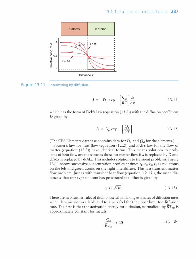
(13.11)
which has the form of Fick’s law (equation (13.8)) with the diffusion coefficientD given by
(13.12)
(The CES Elements database contains data for Do and Qd for the elements.)Fourier’s law for heat flow (equation (12.2)) and Fick’s law for the flow of
matter (equation (13.8)) have identical forms. This means solutions to prob-lems of heat flow are the same as those for matter flow if a is replaced by D anddT/dx is replaced by dc/dx. This includes solutions to transient problems. Figure13.11 shows successive concentration profiles at times t1, t2, t3, t4 as red atomson the left and green atoms on the right interdiffuse. This is a transient matterflow problem. Just as with transient heat flow (equation (12.15)), the mean dis-tance x that one type of atom has penetrated the other is given by
(13.13a)
There are two further rules of thumb, useful in making estimates of diffusion rateswhen data are not available and to give a feel for the upper limit for diffusionrate. The first is that the activation energy for diffusion, normalized by
–RTm, is
approximately constant for metals:
(13.13b)Q
RTd
m
18≈
x Dt≈
D DQ
RTo exp d⎛
⎝⎜⎜⎜⎜
⎞
⎠⎟⎟⎟⎟
J DQ
RTcxo exp
dd
d⎛
⎝⎜⎜⎜⎜
⎞
⎠⎟⎟⎟⎟
13.4 The science: diffusion and creep 287
t2 t1t3t4
t = 0
0
0.5
1
A atoms B atoms
Distance x
Rel
ativ
e co
nc. o
f A
t =
Figure 13.11 Intermixing by diffusion.
Ch13-H8391.qxd 1/16/07 1:42 PM Page 287

The second is that the diffusion coefficient of metals, evaluated at their meltingpoint, is also approximately constant:
(13.13c)
Diffusion in liquids and non-crystalline solidsThe vacancies in a crystal can be thought of as free volume—free because it is ableto move, as it does when an atom jumps. The free volume in a crystal is thus inthe form of discrete units, all of the same size—a size into which an atom withenough thermal energy can jump. Liquids and non-crystalline solids, too, containfree volume, but because there is no lattice or regular structure it is dispersedrandomly between all the atoms or molecules. Experiments show that the energybarrier to atom movement in liquids is not the main obstacle to diffusion or flow.There is actually plenty of free volume among neighbors of any given particle, butit is of little use for particle jumps except when, by chance, it comes together tomake an atom-sized hole—a temporary vacancy. This is a fluctuation problemjust like that of the Maxwell–Boltzmann problem, but a fluctuation of free vol-ume rather than thermal energy, and with a rather similar solution: diffusion inliquids is described by
(13.14)
where vf is the average free volume per particle, va is the volume of the temp-orary vacancy, and ro and v have the same meaning as before.
Diffusion driven by other fieldsSo far we have thought of diffusion driven by a concentration gradient. Con-centration c is a field quantity; it has discrete values at different points in space(the concentration field). The difference in c between two nearby points dividedby the distance between them defines the local concentration gradient, dc/dx.
Diffusion can be driven by other field gradients. A stress gradient, as we shallsee in a moment, drives diffusional flow and power-law creep. An electric fieldgradient can drive diffusion in non-conducting materials. Even a temperaturegradient can drive diffusion of matter as well as diffusion of heat.
Diffusional flowLiquids and hot glasses are wobbly structures, a bit like a bag loosely filled withbeans. If atoms (or beans) move inside the structure, the shape of the whole struc-ture changes in response. Where there is enough free volume, a stress favors themovements that change the shape in the direction of the stress, and opposes thosethat do the opposite, giving viscous flow. The higher the temperature, the moreis the free volume and the faster the flow.
D rv
vo 46
exp2 a
f
ν⎛
⎝⎜⎜⎜⎜
⎞
⎠⎟⎟⎟⎟⎟
D DQ
RToTmd
m
12 2exp m /s ⎛
⎝⎜⎜⎜⎜
⎞
⎠⎟⎟⎟⎟⎟
≈ 10
288 Chapter 13 Running hot: using materials at high temperatures
Ch13-H8391.qxd 1/16/07 1:42 PM Page 288

But how do jumping atoms change the shape of a crystal? A crystal is not likea bag of loose beans—the atoms have well-defined sites on which they sit. Inthe cluster of atoms in Figure 13.9 an atom has jumped but the shape of thecluster has not changed. At first sight, then, diffusion will not change the shapeof a crystal. In fact it does, provided the material is polycrystalline—made upof many crystals meeting at grain boundaries. This is because the grain bound-aries act as sources and sinks for vacancies. If a vacancy joins a boundary, anatom must leave it; repeat this many times and that face of the crystal is eatenaway. If instead a vacancy leaves a boundary, an atom must join it and—repeated—that face grows. Figure 13.12 shows the consequences: the slow exten-sion of the polycrystal in the direction of stress. It is driven by a stress gradient:the difference between the tensile stress σ on the horizontal boundaries fromwhich vacancies flow and that on the others, essentially zero, to which they go.If the grain size is d the stress gradient is σ/d. The flux of atoms, and thus therate at which each grain extends, δd/δt, is proportional to Dσ/d. The strain rate,.ε, is the extension rate divided by the original grain size, d, giving
(13.15)
where C is a constant. This is a sort of viscous flow, linear in stress. The smallerthe grain size, the faster it goes.
ε CDd
Cd
DQ
RToσ σ2 2
dexp⎛
⎝⎜⎜⎜⎜
⎞
⎠⎟⎟⎟⎟
13.4 The science: diffusion and creep 289
Originalshape
Newshape
Stress σ
Grain sized
Diffusing atoms
δdδt
Stress = σ
Stress = 0
Figure 13.12 Deformation by diffusion alone, giving diffusional flow.
Ch13-H8391.qxd 1/16/07 1:42 PM Page 289

Dislocation climb and power-law creepPlastic flow, as we saw in Chapter 5, is the result of the motion of dislocations.Their movement is resisted by dissolved solute atoms, precipitate particles, grainboundaries and other dislocations; the yield strength is the stress needed to forcedislocations past or between them. Diffusion can unlock dislocations from obsta-cles in their path, making it easier for them to move. Figure 13.13 shows howit happens. Here a dislocation is obstructed by a particle. The glide force τb perunit length is balanced by the reaction fo from the precipitate. But if the atomsof the extra half-plane diffuse away, thus eating a slot into the half-plane, thedislocation can continue to glide even though it now has a step in it. The stressgradient this time is less obvious—it is the difference between the local stresswhere the dislocation is pressed against the particle and that on the dislocationremote from it. The process is called ‘climb’ and, since it requires diffusion, it canoccur at a measurable rate only when the temperature is above about 0.35TM.
Climb unlocks dislocations from the obstacles that pin them, allowing furtherslip. After a little slip, of course, the unlocked dislocations encounter the nextobstacles, and the whole cycle repeats itself. This explains the progressive, con-tinuous, nature of creep. The dependence on diffusion explains the dependenceof creep rate on temperature, with
290 Chapter 13 Running hot: using materials at high temperatures
Extra half-plane
Edgedislocation
line
Slip plane
bSlip vector
Extra half-plane
Edgedislocation
line
Slip plane
Diffusion of atoms
Figure 13.13 Climb of a dislocation: the extra half-plane is eaten away by diffusion, allowingthe dislocation to pass the obstacle. The result is power-law creep.
Ch13-H8391.qxd 1/16/07 1:42 PM Page 290

(13.16)
with Qc Qd. The power-law dependence on stress σ is harder to explain. Itarises partly because the stress gradient driving diffusion increases with σ andpartly because the density of dislocations itself increases too.
Deformation mechanism diagramsLet us now pull all this together. Materials can deform by dislocation plasticity(Chapter 6) or, if the temperature is high enough, by diffusional flow or power-lawcreep. If the stress and temperature are too low for any of these, the deformationis elastic. This competition between mechanisms is summarized in deformationmechanism diagrams, of which Figure 13.14 is an example. It shows the rangeof stress and temperature in which we expect to find each sort of deformation andthe strain rate that any combination of them produces (the contours). Diagramslike these are available for many metals and ceramics, and are a useful sum-mary of creep behavior, helpful in selecting a material for high-temperatureapplications—one appears in the examples at the end of this chapter.
Creep fractureDiffusion, we have seen, gives creep. It also gives creep fracture. You mightthink that a creeping material would behave like toffee or chewing gum—that
ε sscexpA
Q
RTnσ
⎛
⎝⎜⎜⎜⎜
⎞
⎠⎟⎟⎟⎟
13.4 The science: diffusion and creep 291
Yielding by dislocation plasticity
Power-law creep
Diffusional flow
Elasticdeformation
T/Tm0 10.5
σ/E
10−5
10−4
10−3
10−1
10−2
Yield strength
1
10
1000
100
Temperature °C
Str
ess,
MP
a
0 200 400 600 800 12001000 1400 1600200200
104
102
1/sec
106
108
1010/sec
3
30
300
0.3
Figure 13.14 A deformation mechanism map, showing the regime in which each mechanismoperates.
Ch13-H8391.qxd 1/16/07 1:42 PM Page 291

it would stretch a long way before breaking in two—but for crystalline materialsthis is very rare. Indeed, creep fracture (in tension) can happen at unexpectedlysmall strains, often only 2–5%, by the mechanism shown in Figure 13.15. Voidsnucleate on grain boundaries that lie normal to the tensile stress. These are theboundaries to which atoms diffuse to give diffusional creep, coming from theboundaries that lie more nearly parallel to the stress. But if the tensile boundarieshave voids on them, they act as sources of atoms too, and in doing so, they grow.The voids cannot support load, so the stress rises on the remaining intact bitsof boundary, making the voids grow more and more quickly until finally (bang)they link.
Many engineering components (e.g. tie-bars in furnaces, super-heater tubes,high-temperature pressure vessels in chemical reaction plants) are expected towithstand moderate creep loads for long times (say 20 years) without failure. Theloads or pressure they can safely carry are calculated by methods such as thosewe have just described. One would like to be able to test new materials for theseapplications without having to wait for 20 years to get the results. It is thustempting to speed up the tests by increasing the load or the temperature to getobservable creep in a short test time, and this is done. But there are risks. Testscarried out on the steep n 3–8 branch of Figure 13.4(a), if extrapolated to lowerstresses where n 1, greatly underestimate the creep rate.
292 Chapter 13 Running hot: using materials at high temperatures
Stress σ
Voids on
boundaries
Void growth by diffusion
Figure 13.15 Creep fracture caused by the diffusive growth of voids on grain boundaries.
Ch13-H8391.qxd 1/16/07 1:42 PM Page 292

Creep mechanisms: polymersCreep in crystalline materials, as we have seen, is closely related to diffusion. Thesame is true of polymers, but because most of them are partly or wholly amor-phous, diffusion is controlled by free volume (equation (13.14)). Free volumeincreases with temperature (its fractional change per degree is just the volumet-ric thermal expansion, 3α) and it does so most rapidly at the glass transitiontemperature Tg. Thus, polymers start to creep as the temperature approachesTg and that, for most, is a low temperature: 50–150°C.
This means that the temperature range in which most polymers are used isthat near Tg when they are neither simple elastic solids nor viscous liquids; theyare visco-elastic solids. If we represent the elastic behavior by a spring and theviscous behavior by a dash-pot, then visco-elasticity (at its simplest) is describedby a coupled spring and dash-pot as in Figure 13.16. Applying a load causes creep,but at an ever-decreasing rate because the spring takes up the tension. Releasingthe load allows slow reverse creep, caused by the extended spring.
Real polymers require more elaborate systems of springs and dash-pots todescribe them. This approach of polymer rheology can be developed to providecriteria for design, but these are complex. A simpler approach is to use graphicaldata for what is called the creep modulus, Ec, to provide an estimate of the defor-mation during the life of the structure. Figure 13.17 shows data for Ec as a func-tion of temperature T and time t. Creep modulus data allow elastic solutions to beused for design against creep. The service temperature and design life are chosen,the resulting creep modulus is read from the graph, and this is used instead ofYoung’s modulus in any of the solutions to design problems listed in Chapter 5.
13.5 Materials to resist creep
Metals and ceramics to resist creepDiffusional flow is important when grains are small (as they often are in ceramics)and when the component is subject to high temperatures at low loads. Equation
13.5 Materials to resist creep 293
SpringDash-pot(damper)
Figure 13.16 Visco-elastic behavior can be modeled as a spring (the elastic part) in parallelwith a dash-pot (the viscous part).
Ch13-H8391.qxd 1/16/07 1:42 PM Page 293
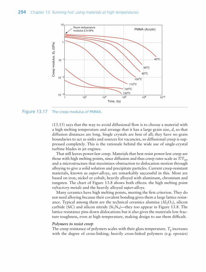
(13.15) says that the way to avoid diffusional flow is to choose a material witha high melting temperature and arrange that it has a large grain size, d, so thatdiffusion distances are long. Single crystals are best of all; they have no grainboundaries to act as sinks and sources for vacancies, so diffusional creep is sup-pressed completely. This is the rationale behind the wide use of single-crystalturbine blades in jet engines.
That still leaves power-law creep. Materials that best resist power-law creep arethose with high melting points, since diffusion and thus creep rates scale as T/Tm,and a microstructure that maximizes obstruction to dislocation motion throughalloying to give a solid solution and precipitate particles. Current creep-resistantmaterials, known as super-alloys, are remarkably successful in this. Most arebased on iron, nickel or cobalt, heavily alloyed with aluminum, chromium andtungsten. The chart of Figure 13.8 shows both effects: the high melting pointrefractory metals and the heavily alloyed super-alloys.
Many ceramics have high melting points, meeting the first criterion. They donot need alloying because their covalent bonding gives them a large lattice resist-ance. Typical among them are the technical ceramics alumina (Al2O3), siliconcarbide (SiC) and silicon nitride (Si3N4)—they too appear in Figure 13.8. Thelattice resistance pins down dislocations but it also gives the materials low frac-ture toughness, even at high temperature, making design to use them difficult.
Polymers to resist creepThe creep resistance of polymers scales with their glass temperature. Tg increaseswith the degree of cross-linking; heavily cross-linked polymers (e.g. epoxies)
294 Chapter 13 Running hot: using materials at high temperatures
1 102 104 106 108 1010103
1
10
102
101
Time, t (s)
Cre
ep m
odul
us, E
c (G
Pa)
40oC
60oC
80oC
100oC
110oC
120oC
130oC
Room temperature modulus 2.9 GPa PMMA (Acrylic)
Figure 13.17 The creep modulus of PMMA.
Ch13-H8391.qxd 1/16/07 1:42 PM Page 294

with high Tg are therefore more creep resistant at room temperature than thosethat are not (like polyethylene). The viscosity of polymers above Tg increaseswith molecular weight, so the rate of creep is reduced by having a high molecularweight. Finally, crystalline or partly crystalline polymers (e.g. high-density poly-ethylene) are more creep resistant than those which are entirely glassy (e.g. low-density polyethylene).
The creep rate of polymers is reduced by filling them with powderedglass, silica (sand) or talc, roughly in proportion to the amount of filler. PTFEon saucepans and polypropylene used for automobile components are bothstrengthened in this way. Much better creep resistance is obtained with com-posites containing chopped or continuous fibers (GFRP and CFRP), becausemuch of the load is now carried by the fibers that, being very strong, do notcreep at all.
Selecting materials to resist creepClasses of industrial applications tend to be associated with certain charac-teristic temperature ranges. There is the cryogenic range, between 273°C androughly room temperature, associated with the use of liquid gases like hydro-gen, oxygen or nitrogen. Here the issue is not creep, but the avoidance of brittlefracture. There is the regime at and near room temperature (20 to 150°C)associated with conventional mechanical and civil engineering: householdappliances, sporting goods, aircraft structures and housing are examples. Abovethis is the range 150–400°C, associated with automobile engines and with foodand industrial processing. Higher still are the regimes of steam turbines andsuperheaters (typically 400–650°C), and of gas turbines and chemical reactors(650–1000°C). Special applications (lamp filaments, rocket nozzles) requirematerials which withstand even higher temperatures, extending as high as2800°C.
Materials have evolved to fill the needs of each of these temperature ranges(Figure 13.18). Certain polymers, and composites based on them, can be usedin applications up to 250°C, and now compete with magnesium and aluminumalloys and with the much heavier cast irons and steels, traditionally used inthose ranges. Temperatures above 400°C require special creep-resistant alloys:ferritic steels, titanium alloys (lighter, but more expensive) and certain stainlesssteels. Stainless steels and ferrous super-alloys really come into their own in thetemperature range above this, where they are widely used in steam turbinesand heat exchangers. Gas turbines require, in general, nickel-based or cobalt-based super-alloys. Above 1000°C, the refractory metals and ceramics becomethe only candidates. Materials used at high temperatures will, generally, per-form perfectly well at lower temperatures too, but are not used there becauseof cost.
The chart of Figure 13.8 showed the performance of materials able to sup-port load at 950°C. Charts like this are used in design in the same way as thosefor low-temperature properties.
13.5 Materials to resist creep 295
Ch13-H8391.qxd 1/16/07 1:42 PM Page 295
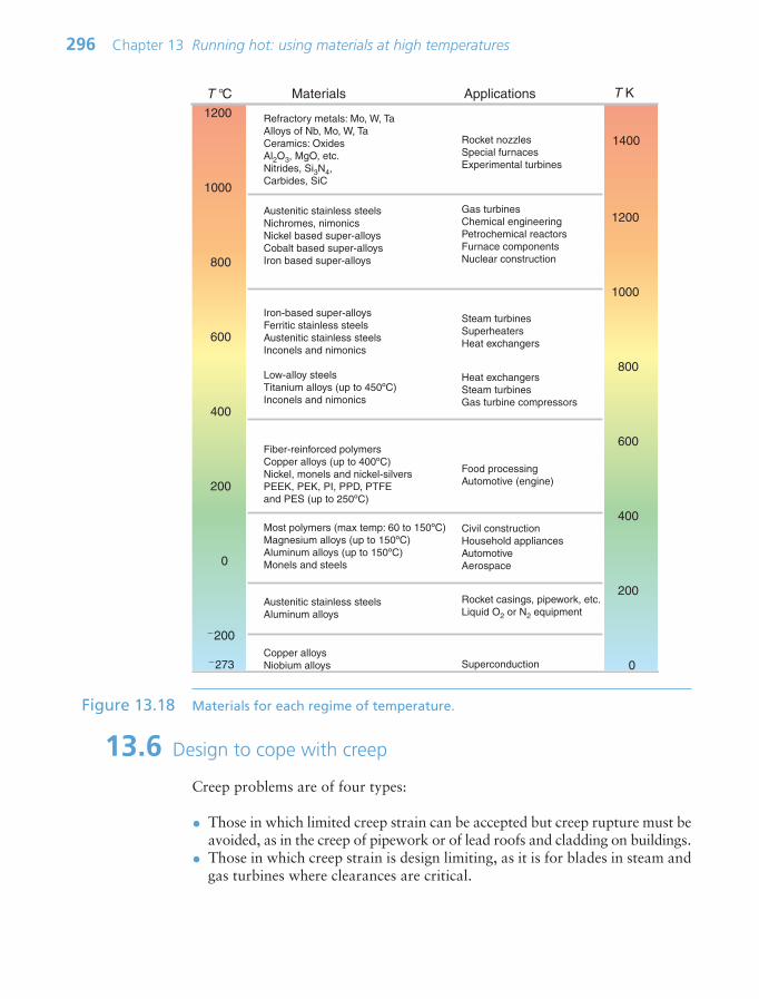
13.6 Design to cope with creep
Creep problems are of four types:
• Those in which limited creep strain can be accepted but creep rupture must beavoided, as in the creep of pipework or of lead roofs and cladding on buildings.
• Those in which creep strain is design limiting, as it is for blades in steam andgas turbines where clearances are critical.
296 Chapter 13 Running hot: using materials at high temperatures
1200
1000
800
600
400
200
0
200
273
Rocket casings, pipework, etc.Liquid O2 or N2 equipment
Superconduction
Civil constructionHousehold appliancesAutomotiveAerospace
Food processingAutomotive (engine)
Heat exchangersSteam turbinesGas turbine compressors
Steam turbinesSuperheatersHeat exchangers
Gas turbinesChemical engineeringPetrochemical reactorsFurnace componentsNuclear construction
Copper alloysNiobium alloys
Austenitic stainless steelsAluminum alloys
Most polymers (max temp: 60 to 150ºC)Magnesium alloys (up to 150ºC)Aluminum alloys (up to 150ºC)Monels and steels
Fiber-reinforced polymersCopper alloys (up to 400ºC)Nickel, monels and nickel-silversPEEK, PEK, PI, PPD, PTFE and PES (up to 250ºC)
Low-alloy steelsTitanium alloys (up to 450ºC)Inconels and nimonics
Iron-based super-alloysFerritic stainless steelsAustenitic stainless steelsInconels and nimonics
Austenitic stainless steelsNichromes, nimonicsNickel based super-alloysCobalt based super-alloysIron based super-alloys
Refractory metals: Mo, W, TaAlloys of Nb, Mo, W, TaCeramics: Oxides Al2O3, MgO, etc.Nitrides, Si3N4, Carbides, SiC
Rocket nozzlesSpecial furnacesExperimental turbines
T °C Materials Applications
1200
1000
800
600
400
200
0
1400
T K
Figure 13.18 Materials for each regime of temperature.
Ch13-H8391.qxd 1/16/07 1:42 PM Page 296

• Those involving more complex problems of creep strain, loss of stiffness andrisk of buckling—a potential problem with space-frames of supersonic air-craft and space vehicles.
• Those involving stress relaxation—the loss of tension in a pre-tightened bolt,for instance.
Predicting life of high temperature pipeworkChemical engineering and power generation plants have pipework that carries hotgases and liquids under high pressure. A little creep, expanding the pipe slightly,can be accepted; rupture, with violent release of hot, high-pressure fluid, cannot.We take, as an example, pipework in a steam-turbine power-generating station.Pipes in a typical 600 MW unit carry steam at 650°C and a pressure p of 15 MPa.The stress in the wall of a thin-walled pipe with a radius R and a wall thickness tcarrying a pressure p, as in Figure 13.19, is
(13.17)
Suppose you have been asked to recommend a pipe required as a temporaryfix while modifications are made to the plant. Space is constrained: the pipecannot be more than 300 mm in diameter. The design life is 6 months. A littlecreep does not matter, but the pipe must not rupture. Type 304 stainless steel pipewith a diameter of 300 mm and a wall thickness of 10 mm is available. Will itfunction safely for the design life?
The stress in the pipe wall with these dimensions, from equation (13.17), is225 MPa. Figure 13.20 shows stress–rupture data for Type 304 stainless steel.Enter 225 MPa at 650°C and read off the rupture life: about 7 hours. Not so good.
So how thick should the pipe be? To find out, reverse the reasoning. The designlife is 6 months—4380 hours. A safety-critical component such as this one needsa safety factor, so double it: 8760 hours. Enter this and the temperature on thestress–rupture plot and read off the acceptable stress: 80 MPa. Put this into
σ pRt
13.6 Design to cope with creep 297
15 MPa650oC
t
2R
σ
Figure 13.19 A pressurized pipe.
Ch13-H8391.qxd 1/16/07 1:42 PM Page 297
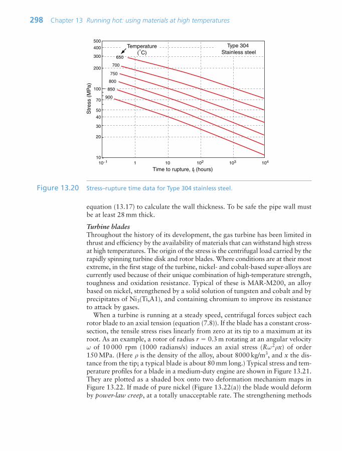
equation (13.17) to calculate the wall thickness. To be safe the pipe wall mustbe at least 28 mm thick.
Turbine bladesThroughout the history of its development, the gas turbine has been limited inthrust and efficiency by the availability of materials that can withstand high stressat high temperatures. The origin of the stress is the centrifugal load carried by therapidly spinning turbine disk and rotor blades. Where conditions are at their mostextreme, in the first stage of the turbine, nickel- and cobalt-based super-alloys arecurrently used because of their unique combination of high-temperature strength,toughness and oxidation resistance. Typical of these is MAR-M200, an alloybased on nickel, strengthened by a solid solution of tungsten and cobalt and byprecipitates of Ni3(Ti,A1), and containing chromium to improve its resistanceto attack by gases.
When a turbine is running at a steady speed, centrifugal forces subject eachrotor blade to an axial tension (equation (7.8)). If the blade has a constant cross-section, the tensile stress rises linearly from zero at its tip to a maximum at itsroot. As an example, a rotor of radius r 0.3 m rotating at an angular velocityω of 10 000 rpm (1000 radians/s) induces an axial stress (Rω2ρx) of order150 MPa. (Here ρ is the density of the alloy, about 8000 kg/m3, and x the dis-tance from the tip; a typical blade is about 80 mm long.) Typical stress and tem-perature profiles for a blade in a medium-duty engine are shown in Figure 13.21.They are plotted as a shaded box onto two deformation mechanism maps inFigure 13.22. If made of pure nickel (Figure 13.22(a)) the blade would deformby power-law creep, at a totally unacceptable rate. The strengthening methods
298 Chapter 13 Running hot: using materials at high temperatures
110−1 102 103 10410
Time to rupture, tf (hours)
Type 304 Stainless steel
20
30
100
10
200
300
400
500
40
70
50Str
ess
(MP
a)
650
700
750
800
850
900
Temperature(°C)
Figure 13.20 Stress–rupture time data for Type 304 stainless steel.
Ch13-H8391.qxd 1/16/07 1:42 PM Page 298

used in MAR-M200 with a typical as-cast grain size of 0.1 mm (Figure 13.22(b))reduce the rate of power-law creep by a factor of 106 and change the dominantmechanism of flow from power-law creep to diffusional flow. Further solutionstrengthening or precipitation hardening is now ineffective unless it slows thismechanism. A new strengthening method is needed: the obvious one is to increase
13.6 Design to cope with creep 299
Root TipBlade
0 10 20 30 40 50Distance (mm)
Str
ess
(MP
a)Te
mpe
ratu
re (
°C)
0
50
100
150
700
800
900
1000
Figure 13.21 A turbine blade, showing the stress and temperature profiles.
Yielding by dislocation plasticity
Power-lawcreep
Diffusional flow
Elasticdeformation
T/Tm0 10.5
σ /E
10−5
10−4
10−3
10−1
10−2
Yield strength
1
10
1000
100
Temperature T, oC
Str
ess
σ, M
Pa
0 400 600 800 12001000 1400200−200
10−4
10−2
1/sec
10−6
10−810−10/sec
3
30
300
0.3
Pure nickelgrain size 0.1mm
MFA 07
Yielding by dislocation plasticity Power-lawcreep
Diffusional flow Elastic
deformation
T/Tm0 10.5
σ /E
10−5
10−4
10−3
10−1
10−2
Yield strength
1
10
1000
100
Temperature T, oC
Str
ess
σ, M
Pa
0 400 600 800 12001000200−200
10−410−2
1/sec
10−6
10−10/sec
3
30
300
0.3
MAR-M200grain size 0.1mm
MFA 07
10−8
10−7
10−9
10000
3000
(a) (b)
Figure 13.22 (a) The stress–temperature profile of the blade plotted onto a deformation mapfor pure nickel. (b) The same profile plotted on a map for the alloy MAR-M200.The strain rates differ by a factor of almost 106.
Ch13-H8391.qxd 1/16/07 1:42 PM Page 299

the grain size or remove grain boundaries altogether by using a single crystal. Thisslows diffusional flow or stops it altogether, while leaving the other flow mech-anisms unchanged. The power-law creep field expands and the rate of creep ofthe turbine blade falls to a negligible level.
The point to remember is that creep has contributions from several distinctmechanisms; the one that is dominant depends on the stress and temperatureapplied to the material. If one is suppressed, another will take its place. Streng-thening methods are selective: a method that works well in one range of stressand temperature may be ineffective in another. A strengthening method shouldbe regarded as a way of attacking a particular flow mechanism. Materials withgood creep resistance combine strengthening mechanisms in order to attack themall; single-crystal MAR-M200 is a good example of this.
Thermal barrier coatingsThe efficiency and power-to-weight ratio of advanced gas turbines, as alreadysaid, is limited by the burn temperature and this in turn is limited by the mate-rials of which the rotor and stator blades are made. Heat enters the blade from theburning gas, as shown in Figure 13.23. Blades are cooled by pumping air throughinternal channels, leading to the temperature profile shown on the left. The sur-face temperature of the blade is set by a balance between the heat transfer coef-ficient between gas and blade (determining the heat in) and conduction within
300 Chapter 13 Running hot: using materials at high temperatures
Thermal barriercoating (TBC)
Bond coat
Super-alloy blade
Coolingchannel
Hot gas
Cooling gas temp.
Burning gas temp.
Temp. profile in blade
Temp. profile in blade
Cooling gas temp.
Burning gas temp.
Tem
pera
ture
Tem
pera
ture
Distance from cooling channel Distance from cooling channel
Heat transfer
Heat transfer
Conduction in blade
Conduction in blade
Conduction in TBC
TBC
Figure 13.23 A cross-section of a turbine blade with a thermal barrier coating (TBC). Thetemperature profile for the uncoated blade is shown on the left, that for thecoated blade on the right.
Ch13-H8391.qxd 1/16/07 1:42 PM Page 300

the blade to the cooling channel (determining the heat out). The temperature stepat the surface is increased by bleeding a trickle of the cooling air through holes inthe blade surface. This technology is already quite remarkable—air-cooled bladesoperate in a gas stream at a temperature that is above the melting point of the alloyof which they are made. How could the burn temperature be increased yet further?
Many ceramics have higher melting points than any metal and some have lowthermal conductivity. Ceramics are not tough enough to make the whole blade,but coating the metal blade with a ceramic to form a thermal barrier coating(TBC) allows an increase in gas temperature with no increase in that of the blade,as shown on the right. How is the ceramic chosen? The first considerations arethose of a low thermal conductivity, a maximum service temperature above thatof the gas (providing some safety margin) and adequate strength. The α–λ chart(Figure 12.4) shows that the technical ceramic with by far the lowest thermalconductivity is zirconia (ZrO2). The Tmax–σf chart (Figure 13.7) confirms that itis usable up to very high temperature and has considerable strength. Zirconialooks like a good bet—and indeed it is this ceramic that is used for TBCs.
As always, it is not quite so simple. Other problems must be overcome tomake a good TBC. It must stick to the blade, and that is not easy. To achieve itthe blade surface is first plated with a thin bond coat (a complex Ni–Cr–Al–Yalloy); it is the glue, so to speak, between blade and coating, shown in Figure13.23. Most ceramics have a lower expansion coefficient than the super-alloy ofthe blade (compare α for ZrO2 and Ni in Figure 12.4) so when the blade heatsup it expands more than the coating and we know what that means: thermalstresses and cracking. The problem is solved (amazingly) by arranging that thecoating is already cracked on a fine scale, with all the cracks running perpendi-cular to its surface, making an array of interlocking columns like a microscopicGiant’s Causeway. When the blade expands the columns separate very slightly,but not enough for hot gas to penetrate to any significant extent; its protectivethermal qualities remain. Next time you fly, reflect on all this—the plane youare in almost certainly has coated blades.
AirframesIf you want to fly at speeds above Mach 1 (760 mph), aerodynamic heatingbecomes a problem. It is easiest to think of a static structure in a wind tunnelwith a supersonic air stream flowing over it. In the boundary layer immediatelyadjacent to the structure, the velocity of the air is reduced to zero and its kineticenergy appears as heat, much of which is dumped into the skin of the structure.The surface temperature Ts can be calculated; it is approximately
Here Ma is the Mach number and To the ambient temperature. Supersonicflight is usually at altitudes above 35 000 ft, where To 50°C. Figure 13.24shows what Ts looks like.
This, not surprisingly, causes problems. First, creep causes a gradual changein dimension over time; wing deflection can increase, affecting aerodynamic
T M Ts a2
o1 0.2≈ ( )
13.6 Design to cope with creep 301
Ch13-H8391.qxd 1/16/07 1:42 PM Page 301

performance. Second, thermal stress caused by expansion can lead to furthercreep damage because it adds to aerodynamic loads. Finally, the drop in modulus,E, brings greater elastic deflection and changes the buckling and flutter (meaningvibration) characteristics.
In a large aircraft, the wing-tip displacement between ground and steady flightis about 0.5 m, corresponding to a strain in the wing-spar (which is loaded inbending) of about 0.1%. To avoid loss of aerodynamic quality, the creep strainover the life of the aircraft must be kept below this. Figure 13.25 illustrates howthe strength of three potential structural materials influences the choice. Where thestrength is flat with temperature (on the left) the material is a practical choice.The temperature at which it drops off limits the Mach number, plotted acrossthe top. Aluminum is light, titanium twice as dense, super-alloys four times so,so increasing the Mach number requires an increase in weight. A heavier structureneeds more power and therefore fuel and fuel, too, has weight—the structuralweight of an aircraft designed to fly at Mach 3 is about three times that of onedesigned for Mach 1. Thus, it appears that there is a practical upper limit on speed.It has been estimated that sustained flight may be limited by the weight penaltyto speeds below Mach 3.5.
Creep relaxationCreep causes pre-tensioned components to relax over time: bolts in hot turbinecasings must be regularly tightened; pipe connectors carrying hot fluids must bereadjusted. It takes only tiny creep strain εcr to relax the stress—a fraction ofthe elastic strain εel caused by pre-tensioning is enough, and εel is seldom muchgreater than 103. Figure 13.26 shows a bolt that is tightened onto a rigid com-ponent so that the initial stress in its shank is σi. The elastic strain is then
εσ
eli
E
302 Chapter 13 Running hot: using materials at high temperatures
−200
0
200
400
600
800
1000
0 1 2 3 4 5Mach number
Adi
abat
ic w
all t
empe
ratu
re
C
Figure 13.24 Adiabatic heating as a function of speed.
Ch13-H8391.qxd 1/16/07 1:42 PM Page 302

If creep strain εcr replaces part of εel the stress relaxes. At any time t
εtot εel εcr
This total strain εtot is fixed because the component on which the bolt is clampedis rigid. Differentiating with respect to time, inserting equation (13.3) for
.εcr gives
13.6 Design to cope with creep 303
0 200 400 600 800 10000
200
400
600
800
10002 3 4 5
Mach number
Temperature (oC)
Tens
ile s
tren
gth
(MP
a)
Al alloys(7075 T6)Density 2800 kg/m3
Ti alloys(Ti–6Al–4V)
Density 4430 kg/m3
Inconel X-750(Ni-based-super-alloy)Density 8250 kg/m3
Figure 13.25 The strength of alloys as a function of temperature.
σ
0 2 4 6 8 100
0.2
0.4
0.6
0.8
1.0
n = 10
n = 4
n = 2
σσi
Time t/to
Figure 13.26 Stress relaxation by creep.
Ch13-H8391.qxd 1/16/07 1:42 PM Page 303

The time t for the stress to relax from σi to σ, for n 1, is found by integratingover time:
Solving for σ/σi as a function of t gives
The stress σ/σi is plotted as a function of t/to in Figure 13.26, for three values of n.The relaxation is most extensive when n is small. As it rises, the drop in stressbecomes less until, as n approaches infinity, meaning rate-independent plasticity,it disappears. Since transient creep is neglected, these curves overestimate therelaxation time for the first tightening of the bolt, but improve for longer times.
13.7 Summary and conclusions
All material properties depend on temperature. Some, like the density and themodulus, change relatively little and in a predictable way, making compensationeasy. Transport properties, meaning thermal conductivity and conductivity formatter flow (which we call diffusion), change in more complex ways. The last ofthese—diffusion—has a profound effect on mechanical properties when temper-atures are high. To understand and use diffusion we need the idea of thermalactivation—the ability of atoms to jump from one site to another, using thermalenergy as the springboard. In crystals, atoms jump from vacancy to vacancy, but inglasses, with no fixed lattice sites, the jumps occur when enough free volume comestogether to make an atom-sized hole. This atom motion allows the intermixing ofatoms in a concentration gradient. External stress, too, drives a flux of atoms,causing the material to change shape in a way that allows the stress to do work.
Diffusion plays a fundamental role in the processing of materials, the subjectof Chapters 18 and 19. It is also diffusion that causes creep and creep fracture.Their rates increase exponentially with temperature, introducing the first chal-lenge for design: that of predicting the rates with useful accuracy. Exponentialrates require precise data—small changes in activation energy give large changesin rates—and these data are hard to measure and are sensitive to slight changesof composition. And there is more than one mechanism of creep, compoundingthe problem. The mechanisms compete, the one giving the fastest rate winning.If you design using data and formulae for one, but under service conditions
σσ
σi
1 i1
1with ( 1)
1
1( / ) /( )t tt n B E
on o
n
tn BE n n
1( )1
1 11
i1σ σ
⎛
⎝⎜⎜⎜⎜
⎞
⎠⎟⎟⎟⎟⎟
ε ε ε tot el cr 0σ
σE
B n
304 Chapter 13 Running hot: using materials at high temperatures
Ch13-H8391.qxd 1/16/07 1:42 PM Page 304

another is dominant, you are in trouble. Deformation mechanism maps helphere, identifying both the mechanism and the approximate rate of creep.
A consequence of all this is that materials selection for high-temperaturedesign, and the design itself, is largely based on empirical data rather than onmodeling of the sort used for elastic and plastic design in Chapters 5, 7 and 10.Empirical data means plots, for individual alloys, of the creep strain rate andlife as functions of temperature and stress. For polymers a different approach is used. Because their melting points and glass temperatures are low, they are visco-elastic at room temperature. Then design can be based on plots of the creep modulus—the equivalent of Young’s modulus for a creeping material.The creep modulus at a given temperature and time is read off the plot and used in standard solutions for elastic problems (Chapter 5) to assess stress ordeflection.
The chapter ends with examples of the use of some of these methods.
13.8 Further reading
Cottrell, A.H. (1964) The Mechanical Properties of Matter, Wiley, London, UK. Libraryof Congress Number 64-14262. (Now 40 years old, inevitably somewhat dated, andnow out of print, but still the best introduction to the mechanical properties of mat-ter that I have ever found. Worth hunting for.)
Finnie, I. and Heller, W.R. (1959) Creep of Engineering Materials, McGraw-Hill, NewYork, USA. Library of Congress No. 58-11171. (Old and somewhat dated, but stillan excellent introduction to creep in an engineering context.)
Frost, H.J. and Ashby, M.F. (1982) Deformation Mechanism Maps, Pergamon Press,Oxford, UK. ISBN 0-08-029337-9. (A monograph compiling deformation mecha-nism maps for a wide range of materials, with explanation of their construction.)
Penny, R.K. and Marriott, D.L. (1971) Design for Creep, McGraw-Hill, New York,USA. ISBN 07-094157-2. (A monograph bringing together the mechanics and thematerials aspects of creep and creep fracture.)
Waterman, N.A. and Ashby, M.F. (1991) The Elsevier Materials Selector, ElsevierApplied Science, Barking, UK. ISBN 1-85166-605-2. (A three-volume compilation ofdata and charts for material properties, including creep and creep fracture.)
13.9 Exercises
13.9 Exercises 305
Exercise E13.1 The self-diffusion constants for aluminum are Do 1.7 104m2/s andQd 142 kJ/mol. What is the diffusion coefficient in aluminum at 400°C?
Exercise E13.2 A steel component is nickel plated to give corrosion protection. To increasethe strength of the bond between the steel and the nickel, the component isheated for 4 hours at 1000°C. If the diffusion parameters for nickel in ironare Do 1.9 104m2/s and Qd 284 kJ/mol, how far would you expectthe nickel to diffuse into the steel in this time?
Ch13-H8391.qxd 1/16/07 1:42 PM Page 305

306 Chapter 13 Running hot: using materials at high temperatures
Exercise E13.3 The diffusion coefficient at the melting point for materials is approximatelyconstant, with the value D 1012m2/s. What is the diffusiondistance if a material is held for 12 hours at just below its melting tempera-ture? This distance gives an idea of the maximum distance over which con-centration gradients can be smoothed by diffusion.
Exercise E13.4 What are the requirements of a creep-resistant material? What materialswould you consider for use at 550°C?
Exercise E13.5 Pipework with a radius of 20 mm and a wall thickness of 4 mm made of 2 1/4Cr Mo steel contains a hot fluid under pressure. The pressure is 10 MPa at atemperature of 600°C. The table lists the creep constants for this steel.Calculate the creep rate of the pipe wall, assuming steady-state power-lawcreep.
Material Reference Reference Rupture Activationstrain stress, σo exponent, energy, Qcrate, .εo (1/s) (MPa) m (kJ/mol)
21/4 Cr Mo steel 3.48 1010 169 7.5 280
Exercise E13.6 There is concern that the pipework described in the previous exercise mightrupture in less than the design life of 1 year. If the Monkman– Grant constantfor 21/4 Cr Mo steel is 0.06, how long will it last before it ruptures?
Exercise E13.7 If the creep rate of a component made of 21/4 Cr Mo steel must not exceed108/second at 500°C, what is the greatest stress that it can safely carry? Usethe data listed in the previous two examples to find out.
Yielding by dislocation plasticity
Power-law creep
Diffusional flow
Elasticdeformation
T/Tm0 10.5
σ/E
10−5
10−4
10−3
10−1
10−2
Yield strength
1
10
1000
100
Temperature °C
Str
ess,
MP
a
0 400 600 800 12001000 1400200−200
10−4
10−2
1/sec
10−-6
10−8
10−10/sec
3
30
300
0.3
Stainless steel grain size 10 µm
Ch13-H8391.qxd 1/16/07 1:42 PM Page 306

13.9 Exercises 307
Exercise E13.8 A stainless steel suspension cable in a furnace is subjected to a stress of100 MPa at 700°C. Its creep rate is found to be unacceptably high. By whatmechanism is creep occurring? What action would you suggest to tackle theproblem? The figure shows the deformation mechanism map for the material.
Exercise E13.9 The wall of a pipe of the same stainless steel as that of the previous exercisecarries a stress of 3 MPa at the very high temperature of 1000°C. In this appli-cation it, too, creeps at a rate that is unacceptably high. By what mechanismis creep occurring? What action would you suggest to tackle the problem?
Exercise E13.10 It is proposed to make a shelf for a hot-air drying system from acrylic sheet.The shelf is simply supported, as in the diagram, and has a width w 500 mm,a thickness t 8 mm and a depth b 200 mm. It must carry a distributedload of 50 N at 60°C with a design life of 800 hours(about a year) of continuous use. Use the creepmodulus plotted in Figure 13.17 and the solution tothe appropriate elastic problem (Chapter 5) to findout how much it will sag in that time. w
F
tδ
Ch13-H8391.qxd 1/16/07 1:42 PM Page 307

308 Chapter 13 Running hot: using materials at high temperatures
Exercise E13.15 The claim is made in the text (equation (13.13b)) that the activation energyfor self-diffusion, normalized by
–RTm, is approximately constant for metals:
Make a bar chart of this quantity and explore the degree to which it is true.
Exercise E13.16 The claim is made in the text (equation (13.13c)) that the diffusion coefficientof metals, evaluated at their melting point, is also approximately constant:
D DQ
RToTmd
m
12 2exp m /s ⎛
⎝⎜⎜⎜⎜
⎞
⎠⎟⎟⎟⎟⎟
≈ 10
Q
RTd
m
18≈
13.11 Exploring the science with CES Elements
13.10 Exploring design with CES (use Level 2 unless otherwisestated)
Exercise E13.11 Use the Search facility in CES to find:
(a) Materials for turbine blades.(b) Materials for thermal barrier coatings.
Exercise E13.12 Use the CES software to make a bar chart for the glass temperatures ofpolymers like that for melting point in the text (Figure 13.6). What is therange of glass temperatures for polymers?
Exercise E13.13 The analysis of thermal barrier coatings formulated the design constraints.Use the selector to find the best material. Here is a summary of the con-straints and the objective.
Function • Thermal barrier coating
Constraints • Maximum service temperature 1300°C• Adequate strength: σy 400 MPa
Objective • Minimize thermal conductivity λ
Free variable • Choice of material
Exercise E13.14 Find materials with Tmax 500°C and the lowest possible thermal conduc-tivity. Switch the database to Level 3 to get more detail. Report the threematerials with the lowest thermal conductivity.
Ch13-H8391.qxd 1/16/07 1:42 PM Page 308

13.11 Exploring the science with CES Elements 309
Make a bar chart of this quantity and explore the degree to which it is true.
Exercise E13.17 What is a ‘typical’ value for the pre-exponential, Do? Is it roughly constantfor the elements? Make a chart with the activation energy for diffusion, Qd,on the x-axis and the pre-exponential Do on the y-axis to explore this.
Exercise E13.18 The diffusive jump shown in Figure 13.9 requires that the diffusing atombreaks its bonds in its starting position in order to jump into its final one.You might, then, expect that there would be at least an approximate pro-portionality between the activation energy for self-diffusion Qd and thecohesive energy Hc of the material. Make a chart with Hc on the x-axis andQd on the y-axis. Report what you find.
Ch13-H8391.qxd 1/16/07 1:42 PM Page 309

This page intentionally left blank
Chapter 14Conductors, insulators
and dielectrics
Chapter contents
14.1 Introduction and synopsis 31214.2 Conductors, insulators and dielectrics 31314.3 Charts for electrical properties 31714.4 Drilling down: the origins and
manipulation of electrical properties 32014.5 Design: using the electrical properties
of materials 33114.6 Summary and conclusions 33814.7 Further reading 33814.8 Exercises 33914.9 Exploring design with CES 34114.10 Exploring the science with
CES Elements 343
Conductors and insulators. Copper, aluminum andsilver (if you can afford it) make good conductors.Pyrex, porcelain and ceramics like alumina makegood insulators – they are dielectrics. (Images
courtesy of the Copper Development Association.)
Ch14-H8391.qxd 1/16/07 6:10 PM Page 311
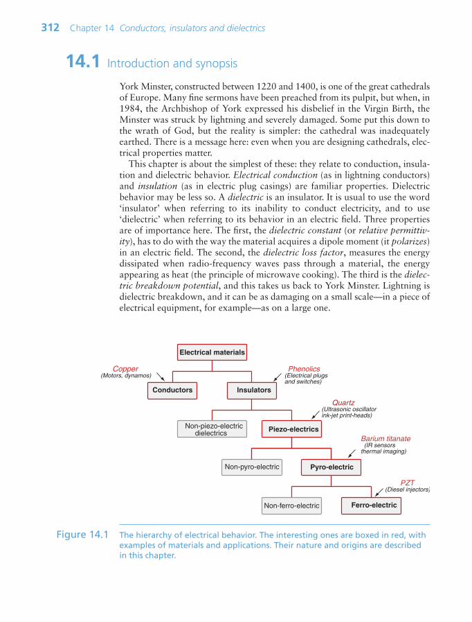
312 Chapter 14 Conductors, insulators and dielectrics
14.1 Introduction and synopsis
York Minster, constructed between 1220 and 1400, is one of the great cathedralsof Europe. Many fine sermons have been preached from its pulpit, but when, in1984, the Archbishop of York expressed his disbelief in the Virgin Birth, theMinster was struck by lightning and severely damaged. Some put this down tothe wrath of God, but the reality is simpler: the cathedral was inadequatelyearthed. There is a message here: even when you are designing cathedrals, elec-trical properties matter.
This chapter is about the simplest of these: they relate to conduction, insula-tion and dielectric behavior. Electrical conduction (as in lightning conductors)and insulation (as in electric plug casings) are familiar properties. Dielectricbehavior may be less so. A dielectric is an insulator. It is usual to use the word‘insulator’ when referring to its inability to conduct electricity, and to use‘dielectric’ when referring to its behavior in an electric field. Three propertiesare of importance here. The first, the dielectric constant (or relative permittiv-ity), has to do with the way the material acquires a dipole moment (it polarizes)in an electric field. The second, the dielectric loss factor, measures the energydissipated when radio-frequency waves pass through a material, the energyappearing as heat (the principle of microwave cooking). The third is the dielec-tric breakdown potential, and this takes us back to York Minster. Lightning isdielectric breakdown, and it can be as damaging on a small scale—in a piece ofelectrical equipment, for example—as on a large one.
Electrical materials
Conductors Insulators
Non-piezo-electric dielectrics Piezo-electrics
Non-pyro-electric Pyro-electric
Non-ferro-electric Ferro-electric
Phenolics(Electrical plugs and switches)
Quartz(Ultrasonic oscillatorink-jet print-heads)
PZT(Diesel injectors)
Barium titanate (IR sensorsthermal imaging)
Copper(Motors, dynamos)
Figure 14.1 The hierarchy of electrical behavior. The interesting ones are boxed in red, withexamples of materials and applications. Their nature and origins are describedin this chapter.
Ch14-H8391.qxd 1/16/07 6:10 PM Page 312

14.2 Conductors, insulators and dielectrics 313
There are many different kinds of electrical behavior, all of them useful.Figure 14.1 gives an overview, with examples of materials and applications.The chapter introduces electrical properties and their physical origins, andexamples of design for electrical performance.
14.2 Conductors, insulators and dielectrics
Resistivity and conductivityThe electrical resistance R (units: ohms,1 symbol Ω) of a rod of material is thepotential drop V (volts2) across it, divided by the current i (amps3) passingthrough it, as in Figure 14.2. This relationship is Ohm’s law:
(14.1)
The material property that determines resistance is the electrical resistivity, ρe.It is related to the resistance by
(14.2) eAL
R
RVi
Pot
entia
l diff
eren
ce V
Current
Resistance R = V/
Current
Area A
VL
Resistivity
ρe = A
LR
+
−
i.
i.
i.
Figure 14.2 Electrical resistivity, ρe. Its value ranges from 1 to 1024 µΩ.cm.
1 George Simon Ohm (1787–1854), dropped out of his studies at the University of Erlangen,preferring billiards to mathematics, but later became absorbed in the theory of electricityand magnetism.
2 Alessandro Guiseppe Antonio Anastasio Volta (1745–1827), Italian physicist, inventor ofthe battery or, as it was then known, the Voltaic Pile. His face used to appear on the10 000 lire note.
3 André Marie Ampère (1775–1836), mathematician and physicist, who, it was said, hadmastered all known mathematics by the age of 14. His life was not a happy one: fatherguillotined during the French Revolution, miserably married and with difficult children—yet he remained extensively productive up to his death.
Ch14-H8391.qxd 1/16/07 6:10 PM Page 313

where A is the section and L the length of a test rod of material—think of it asthe resistance of a unit cube of the material. Its units in the metric system areΩ.m, but it is commonly reported in units of µΩ.cm. It has an immense range,from a little more than 108 in units of Ω.m for good conductors (equivalent to 1 µΩ.cm, which is why these units are still used) to more than 1016Ω.m (1024 µΩ.cm) for the best insulators. The electrical conductivity κe is simply thereciprocal of the resistivity. Its units are siemens per meter S/m or (Ω.m)1).
Dielectric propertiesFirst, a reminder of what is meant by a field: it is a region of space in which objectsexperience forces if they have the right properties. Charge creates an electric field,E. The electric field strength between two oppositely charged plates separated bya distance t and with a potential difference V between them is
(14.3)
and is independent of position except near the edge of the plates.Two conducting plates separated by a dielectric make a capacitor (Figure 14.3).
Capacitors (sometimes called condensers) store charge. The charge Q (coulombs4)is directly proportional to the potential difference between the plates, V (volts):
Q CV (14.4)
EVt
314 Chapter 14 Conductors, insulators and dielectrics
t
Cha
rge
Q
Capacity C = Q/V
Charge Q
Dielectric material
Dielectric constant
εr = C (dielectric in place)
C (no dielectric)
Potential difference V
*Breakdown
Area A
V
+
−
Figure 14.3 Dielectric constant and dielectric breakdown. The capacitance of a condenser isproportional to the dielectric constant, and the maximum charge it can hold islimited by breakdown.
4 Charles Augustin Coulomb (1736–1806), military physicist, laid the foundations of both themathematical description of electrostatic forces and the laws of friction. Despite his appoint-ment as Intendant des Eaux et Fontaines de Paris, he made no known contributions to hydro-dynamics.
Ch14-H8391.qxd 1/16/07 6:10 PM Page 314
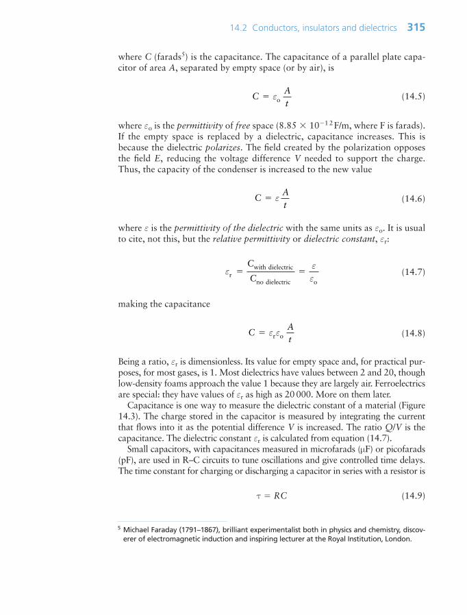
where C (farads5) is the capacitance. The capacitance of a parallel plate capa-citor of area A, separated by empty space (or by air), is
(14.5)
where εo is the permittivity of free space (8.85 101 2F/m, where F is farads).If the empty space is replaced by a dielectric, capacitance increases. This isbecause the dielectric polarizes. The field created by the polarization opposesthe field E, reducing the voltage difference V needed to support the charge.Thus, the capacity of the condenser is increased to the new value
(14.6)
where ε is the permittivity of the dielectric with the same units as εo. It is usualto cite, not this, but the relative permittivity or dielectric constant, εr:
(14.7)
making the capacitance
(14.8)
Being a ratio, εr is dimensionless. Its value for empty space and, for practical pur-poses, for most gases, is 1. Most dielectrics have values between 2 and 20, thoughlow-density foams approach the value 1 because they are largely air. Ferroelectricsare special: they have values of εr as high as 20 000. More on them later.
Capacitance is one way to measure the dielectric constant of a material (Figure14.3). The charge stored in the capacitor is measured by integrating the currentthat flows into it as the potential difference V is increased. The ratio Q/V is thecapacitance. The dielectric constant εr is calculated from equation (14.7).
Small capacitors, with capacitances measured in microfarads (µF) or picofarads(pF), are used in R–C circuits to tune oscillations and give controlled time delays.The time constant for charging or discharging a capacitor in series with a resistor is
τ RC (14.9)
CAt
ε εr o
εεεr
with dielectric
no dielectric o
C
C
CAt
ε
CAt
εo
14.2 Conductors, insulators and dielectrics 315
5 Michael Faraday (1791–1867), brilliant experimentalist both in physics and chemistry, discov-erer of electromagnetic induction and inspiring lecturer at the Royal Institution, London.
Ch14-H8391.qxd 1/16/07 6:10 PM Page 315
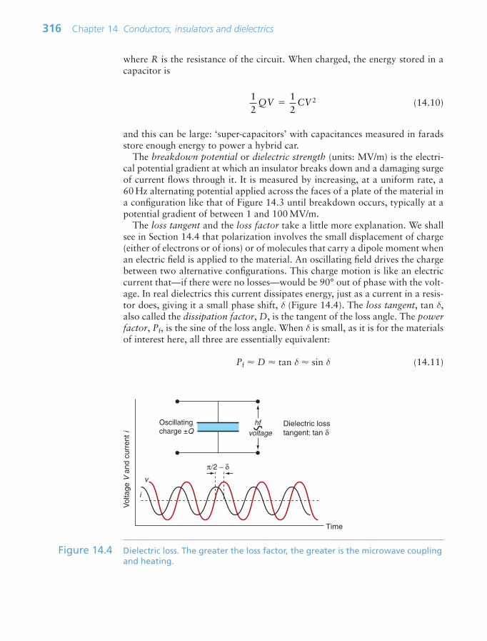
where R is the resistance of the circuit. When charged, the energy stored in acapacitor is
(14.10)
and this can be large: ‘super-capacitors’ with capacitances measured in faradsstore enough energy to power a hybrid car.
The breakdown potential or dielectric strength (units: MV/m) is the electri-cal potential gradient at which an insulator breaks down and a damaging surgeof current flows through it. It is measured by increasing, at a uniform rate, a60 Hz alternating potential applied across the faces of a plate of the material ina configuration like that of Figure 14.3 until breakdown occurs, typically at apotential gradient of between 1 and 100 MV/m.
The loss tangent and the loss factor take a little more explanation. We shallsee in Section 14.4 that polarization involves the small displacement of charge(either of electrons or of ions) or of molecules that carry a dipole moment whenan electric field is applied to the material. An oscillating field drives the chargebetween two alternative configurations. This charge motion is like an electriccurrent that—if there were no losses—would be 90° out of phase with the volt-age. In real dielectrics this current dissipates energy, just as a current in a resis-tor does, giving it a small phase shift, δ (Figure 14.4). The loss tangent, tan δ,also called the dissipation factor, D, is the tangent of the loss angle. The powerfactor, Pf, is the sine of the loss angle. When δ is small, as it is for the materialsof interest here, all three are essentially equivalent:
Pf D tan δ sin δ (14.11)
12
12
2QV CV
316 Chapter 14 Conductors, insulators and dielectrics
Vol
tage
V a
nd c
urre
nt i
Dielectric losstangent: tan δ
Oscillatingcharge ±Q
hfvoltage
v
i
π/2 − δ
Time
Figure 14.4 Dielectric loss. The greater the loss factor, the greater is the microwave couplingand heating.
Ch14-H8391.qxd 1/16/07 6:10 PM Page 316

More useful, for our purposes, is the loss factor L, which is the loss tangenttimes the dielectric constant:
L εr tan δ (14.12)
It measures the energy dissipated in a dielectric when in an oscillating field. Ifyou want to select materials to minimize or maximize dielectric loss, then themeasure you want is L.
When a dielectric material is placed in a cyclic electric field of amplitude Eand frequency f, power P is dissipated and the field is correspondingly attenu-ated. The power dissipated per unit volume, in W/m3, is
P f E2 ε tan δ f E2 εo εr tan δ f E2 εo L (14.13)
where, as before, εr is the dielectric constant of the material and tan δ is its losstangent. This power appears as heat and is generated uniformly through thevolume of the material. Thus, the higher the frequency or the field strength andthe greater the loss factor εr tan δ, the greater is the heating and energy loss.This dielectric loss is exploited in processing—for example, in radio-frequencywelding of polymers.
All dielectrics change shape in an electric field, a consequence of the small shiftin charge that allows them to polarize; the effect is called electrostriction.Electrostriction is a one-sided relationship in that an electric field causes deforma-tion, but deformation does not produce an electric field. Piezo-electric materials,by contrast, display a two-sided relationship between polarization and deforma-tion: a field induces deformation and deformation induces charge differencesbetween its surfaces, thus creating a field. The piezo-electric coefficient is thestrain per unit of electric field, and although it is very small, it is a true lineareffect, and this makes it useful: when you want to position or move a probe withnanoscale precision it is just what you need. Pyro-electric materials contain mol-ecules with permanent dipole moments that, in a single crystal, are aligned, giv-ing the crystal a permanent polarization. When the temperature is changed thepolarization changes, creating surface charges or, if the surfaces are connectedelectrically, a pyro-electric current—the principle of intruder detection systemsand of thermal imaging. Ferro-electric materials, too, have a natural dipolemoment—they are polarized to start with, and the individual polarized moleculesline up so that their dipole moments are parallel, like magnetic moments in amagnet. Their special feature is that the direction of polarization can be changedby applying an electric field, and the change causes a change of shape.Applications of all of these are described in Section 14.5.
14.3 Charts for electrical properties
All materials have an electrical resistivity and all dielectrics have a dielectricconstant and loss factor. Property charts for these are useful because they allow
14.3 Charts for electrical properties 317
Ch14-H8391.qxd 1/16/07 6:10 PM Page 317
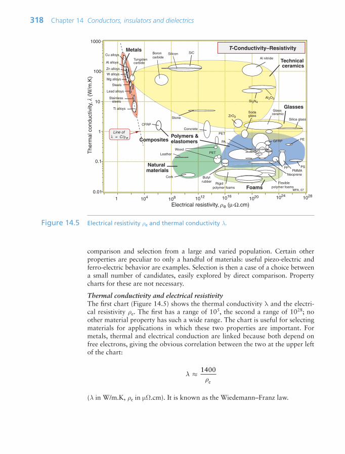
comparison and selection from a large and varied population. Certain otherproperties are peculiar to only a handful of materials: useful piezo-electric andferro-electric behavior are examples. Selection is then a case of a choice betweena small number of candidates, easily explored by direct comparison. Propertycharts for these are not necessary.
Thermal conductivity and electrical resistivityThe first chart (Figure 14.5) shows the thermal conductivity λ and the electri-cal resistivity ρe. The first has a range of 105, the second a range of 1028; noother material property has such a wide range. The chart is useful for selectingmaterials for applications in which these two properties are important. Formetals, thermal and electrical conduction are linked because both depend onfree electrons, giving the obvious correlation between the two at the upper leftof the chart:
(λ in W/m.K, ρe in µΩ.cm). It is known as the Wiedemann–Franz law.
λρ
≈1400
e
318 Chapter 14 Conductors, insulators and dielectrics
ZrO2
Foams
Polymers &elastomers
Metals
Technical ceramics
Composites
Natural materials
Lead alloys
W alloys
Steels
Ti alloys
Mg alloys
CFRP
GFRP
Al alloys
Rigid polymer foams
Flexible polymer foams
Cu alloys
Zn alloys
PA
PMMA
PET
PET
Cork
Wood
Butyl rubber
Concrete
Tungstencarbide
Al2O3
SiC
Si3N4
T-Conductivity–Resistivity
Stainless steels
Al nitrideSilicon
PP PS
PE
Glass ceramic
Leather
Boron carbide
Neoprene
1000
100
10
1
0.1
0.01
1 104 108 1012 1016 1020 1024 1028
Electrical resistivity, ρe (µ-Ω.cm)
The
rmal
con
duct
ivity
, λ (
W/m
.K)
Stone
Glasses
Silica glass
Soda glass
Line of λ = C/ρe
MFA, 07
Figure 14.5 Electrical resistivity ρe and thermal conductivity λ.
Ch14-H8391.qxd 1/16/07 6:10 PM Page 318

Strength and electrical resistivityThe second chart (Figure 14.6) shows electrical resistivity ρe and strength σel.Metals lie at the extreme left: copper and silver (not shown) have the lowest resis-tivities, with aluminum only just above. The strongest alloys have resistivities thatare 10–100 times larger. Ceramics such as alumina, aluminum nitride and silica,at the upper right, have very high resistivities and are strong; they are used formaking insulators for power lines and substrates for electronic circuitry. Belowthem lie polymers that are less strong, but are flexible, easily molded and excel-lent insulators; they are used for cable sheathing, insulation of switch gear andthe like.
Strength and dielectric lossThe final chart (Figure 14.7) shows dielectric loss factor L and strength σy or σel. Materials that are transparent to microwaves (radar uses microwave frequencies) lie at the left: polymer foams, certain polymers (PP, PE, PTFE) and some ceramics have particularly low values. Materials that absorbmicrowaves, becoming hot in the process, lie at the right: polymers containinga polar group, like nylon and polyurethane, and natural materials like woods(woods are dried by microwave heating). Water, which has a polar molecule,
14.3 Charts for electrical properties 319
Stre
ngth
σy
or σ
el (M
Pa)
0.01
0.1
1
10
100
1000
10 000
1 103 106 109 1012 10181015 1021 1024 1028
Electrical resistivity, ρe (µΩ.cm)
Foams
Polymersand
elastomers
MetalsTechnical ceramics
Natural materials
Lead alloys
Brass
SteelsTi alloys
Mg alloys
CFRP
GFRP
Al alloys
Rigid polymer foams
Flexible polymer foams
Cu alloys
Zn alloys
PA
PMMA
PC
Cork
Wood
ZrO2
Al2O3
SiC Si3N4
Strength–Resistivity
Stainless steels
Al nitride
Silicon
PP
PS
PE
Leather
Boron carbide
Neoprene
Stone
Glasses
Silica glass
Soda glass
MFA, 07
Ni alloys
PTFE
ABS
EpoxyPhenolic
Figure 14.6 Material property chart for electrical resistivity ρe and yield strength σy or elasticlimit σel.
Ch14-H8391.qxd 1/16/07 6:10 PM Page 319

has a particularly large loss factor, which is why most foods can be cooked in amicrowave oven.
14.4 Drilling down: the origins and manipulation of electricalproperties
Electrical conductivityAn electric field, E (volts/m), exerts a force Ee on a particle carrying a charge.Solids are made up of atoms containing electrons that carry a charge e and anucleus containing protons, each with a positive charge e. If charge carrierscan move, the force Ee causes them to flow through the material—that is, itconducts. Metals are electron conductors, meaning that the charge carriers arethe electrons. In ionic solids (which are composed of negatively and positivelycharged ions like Na Cl) the diffusive motion of ions allows ionic conduc-tion, but this is only possible at temperatures at which diffusion is rapid. Manymaterials have no mobile electrons, and at room temperature they are too cold
320 Chapter 14 Conductors, insulators and dielectrics
Dielectric loss factor εr tan δ10−4 10−3 10−2 10−1 1
0.01
0.1
1
10
100
1000
10 000
Foams
Polymers and elastomers
Technical ceramics
Natural materials
GFRP
Rigid polymerfoams
Flexible polymer
foams
NylonsPMMA
PTFE
Cork
Wood
Butyl rubber
Concrete
Al2O3 SiCSi3N4
Strength–Dielectric loss
Al nitride
PP
PU
PE
Boron carbide
Neoprene
Stone
Silica glass
Soda glass
MFA, 07
ZrO2
Isoprene
PS ABSPC
PEEKEpoxy
Stre
ngth
σy
or σ
el (M
Pa)
Figure 14.7 Material property chart for dielectric loss, εr tan δ and yield strength σy or elasticlimit σel.
Ch14-H8391.qxd 1/16/07 6:10 PM Page 320
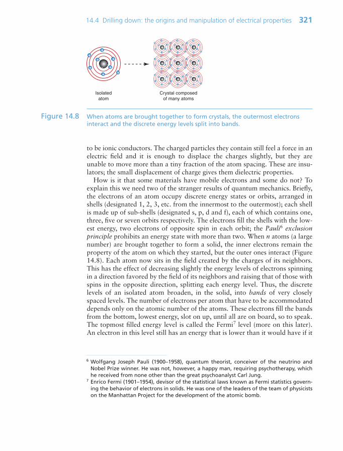
to be ionic conductors. The charged particles they contain still feel a force in anelectric field and it is enough to displace the charges slightly, but they areunable to move more than a tiny fraction of the atom spacing. These are insu-lators; the small displacement of charge gives them dielectric properties.
How is it that some materials have mobile electrons and some do not? Toexplain this we need two of the stranger results of quantum mechanics. Briefly,the electrons of an atom occupy discrete energy states or orbits, arranged inshells (designated 1, 2, 3, etc. from the innermost to the outermost); each shellis made up of sub-shells (designated s, p, d and f), each of which contains one,three, five or seven orbits respectively. The electrons fill the shells with the low-est energy, two electrons of opposite spin in each orbit; the Pauli6 exclusionprinciple prohibits an energy state with more than two. When n atoms (a largenumber) are brought together to form a solid, the inner electrons remain theproperty of the atom on which they started, but the outer ones interact (Figure14.8). Each atom now sits in the field created by the charges of its neighbors.This has the effect of decreasing slightly the energy levels of electrons spinningin a direction favored by the field of its neighbors and raising that of those withspins in the opposite direction, splitting each energy level. Thus, the discretelevels of an isolated atom broaden, in the solid, into bands of very closelyspaced levels. The number of electrons per atom that have to be accommodateddepends only on the atomic number of the atoms. These electrons fill the bandsfrom the bottom, lowest energy, slot on up, until all are on board, so to speak.The topmost filled energy level is called the Fermi7 level (more on this later). An electron in this level still has an energy that is lower than it would have if it
14.4 Drilling down: the origins and manipulation of electrical properties 321
Isolatedatom
Crystal composedof many atoms
Figure 14.8 When atoms are brought together to form crystals, the outermost electronsinteract and the discrete energy levels split into bands.
6 Wolfgang Joseph Pauli (1900–1958), quantum theorist, conceiver of the neutrino andNobel Prize winner. He was not, however, a happy man, requiring psychotherapy, whichhe received from none other than the great psychoanalyst Carl Jung.
7 Enrico Fermi (1901–1954), devisor of the statistical laws known as Fermi statistics govern-ing the behavior of electrons in solids. He was one of the leaders of the team of physicistson the Manhattan Project for the development of the atomic bomb.
Ch14-H8391.qxd 1/16/07 6:10 PM Page 321

were isolated in a vacuum far from the atoms. This energy difference is called,for historical reasons, the work function because it is the work that you have todo to remove an electron from the Fermi level to infinity. If you want to createan electron beam by pulling electrons out of a metal by using a high electricfield (called a field-emission electron gun) you have to provide the work func-tion to do it.
Whether the material is a conductor or an insulator depends on how full thebands are, and whether or not they overlap. In Figure 14.9 the central columndescribes an isolated atom and the outer ones illustrate the possibilities createdby bringing atoms together into an array, with the energies spread into energybands. Conductors like copper, shown on the left, have an unfilled outer band; there are many very closely spaced levels just above the last full one,and—when accelerated by a field—electrons can use these levels to move freelythrough the material. In insulators, shown on the right, the outermost bandwith electrons in it is full, and the nearest empty band is separated from it in energy by a wide band gap. Semiconductors, too, have a band gap, but it is narrower—narrow enough that thermal energy can pop a few electrons into the empty band, where they conduct. Deliberate doping (adding trace lev-els of impurities) creates new levels in the band gap, reducing the energy bar-rier to entering the empty states and thus allowing more carriers to becomemobile.
Electrical resistanceIf a field E exerts a force Ee on an electron, why does it not accelerate forever,giving a current that continuously increases with time? This is not what hap-pens; instead, switching on a field causes a current that almost immediately
322 Chapter 14 Conductors, insulators and dielectrics
Electronicconductor
Insulator(dielectric)
Unsplitlevels
Unsplitlevels
Filledband
Filledband
Partlyfilledband
Bandgap
Isolatedatom
Energy
Empty
Filled
Filled
Filled
Filled
Figure 14.9 Conductors, on the left, have a partly filled outer band—electrons in it canmove easily. Insulators, on the right, have an outer filled band, separated fromthe nearest unfilled band by a band gap. (Red bands are filled, blue bands areempty.)
Ch14-H8391.qxd 1/16/07 6:10 PM Page 322
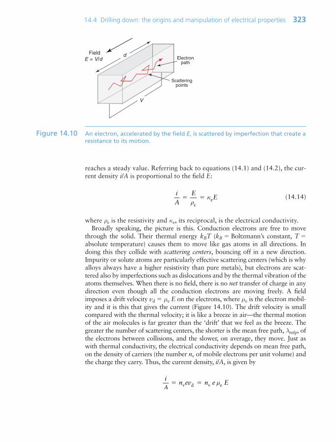
reaches a steady value. Referring back to equations (14.1) and (14.2), the cur-rent density i/A is proportional to the field E:
(14.14)
where ρe is the resistivity and κe, its reciprocal, is the electrical conductivity.Broadly speaking, the picture is this. Conduction electrons are free to move
through the solid. Their thermal energy kBT (kB Boltzmann’s constant, T absolute temperature) causes them to move like gas atoms in all directions. Indoing this they collide with scattering centers, bouncing off in a new direction.Impurity or solute atoms are particularly effective scattering centers (which is whyalloys always have a higher resistivity than pure metals), but electrons are scat-tered also by imperfections such as dislocations and by the thermal vibration of theatoms themselves. When there is no field, there is no net transfer of charge in anydirection even though all the conduction electrons are moving freely. A fieldimposes a drift velocity vd µe E on the electrons, where µe is the electron mobil-ity and it is this that gives the current (Figure 14.10). The drift velocity is smallcompared with the thermal velocity; it is like a breeze in air—the thermal motionof the air molecules is far greater than the ‘drift’ that we feel as the breeze. Thegreater the number of scattering centers, the shorter is the mean free path, λmfp, ofthe electrons between collisions, and the slower, on average, they move. Just aswith thermal conductivity, the electrical conductivity depends on mean free path,on the density of carriers (the number nv of mobile electrons per unit volume) andthe charge they carry. Thus, the current density, i/A, is given by
iA
n ev n e E v d v eµ
iA
EE
ρκ
ee
14.4 Drilling down: the origins and manipulation of electrical properties 323
V
V/d Field E =
d Electronpath
Scatteringpoints
Figure 14.10 An electron, accelerated by the field E, is scattered by imperfection that create aresistance to its motion.
Ch14-H8391.qxd 1/16/07 6:10 PM Page 323

Comparing this with equation (14.14) gives the conductivity:
κe nv e µe (14.15)
Thus the conductivity is proportional to the density of free electrons and to theelectron mobility, and this is directly proportional to the mean free path. Thepurer and more perfect the conductor, the higher is the conductivity.
Metals are strengthened (Chapter 7) by solid solution hardening, work harden-ing or precipitation hardening. All of these change the resistivity too. By ‘zoomingin’ on part of the strength–resistivity chart, we can see how both properties areaffected—Figure 14.11 shows this for two of the best conductors: copper and alu-minum. Adding solute to either metal increases its solute atoms also act as scatter-ing centers, increasing the electrical resistivity too. Dislocations add strength (bywhat we called work hardening) and they too scatter electrons a little, though notas much as solute. Precipitates offer the greatest gain in strength; their effect onresistivity varies, depending on their size and spacing compared to the electronmean free path and on the amount of residual solute left in the lattice. Precipitationhardening (with low residual solute) or work hardening are therefore the best waysto strengthen conductors. The two figures show that commercial conductor alloyshave much greater strength, and only slightly greater resistivity than the puremetals.
The resistivity of metals increases with temperature because thermal vibrationscatters electrons. Resistance decreases as temperature falls, which is why very-high-powered electromagnets are pre-cooled in liquid nitrogen. As absolute zero
324 Chapter 14 Conductors, insulators and dielectrics
Yie
ld s
treng
th,
tens
ion
(MP
a)
Electrical resistivity (µohm.cm)1 2 5 10 20 50
20
100
1000
Wor
kha
rden
ing
Precip
itate
har
deni
ng
Solute hardening
Copper–beryllium
Pure, softcopper
Hard drawncopper
Brasses,bronzes,
soft
Brasses,bronzes,
hard drawn
Copper–nickel,
soft
Copper–nickel,
hard drawn
Copper alloys
Work
hard
enin
g
Conductormaterials
Yie
ld s
treng
th,
tens
ion
(MP
a)
10
100
1000
Electrical resistivity (µohm.cm)1 2 5 10
Aluminum alloys
Wor
kha
rden
ing
Pure, softaluminum
Wrought(1050 H9)
Al–Si–Mg–Mn(6082 T6)
Al–Cu–Mg(2024 T861)
Al–Zn–Mg–Cu(7075 T6)
Al–Mg, soft(5083 H0)
Al–Mg, wrought(5083 H343)
Pre
cipi
tate
har
deni
ng
Solute harde
ning
Conductormaterials
Figure 14.11 The best choice of material for a cable is one with high strength and lowresistivity, but strengthening mechanisms increase resistivity. Work hardeningand precipitation hardening do so less than solute hardening.
Ch14-H8391.qxd 1/16/07 6:10 PM Page 324

is approached most metals retain some resistivity, but a few, at between 0 and4 K, suddenly lose all resistance and become superconducting. The resistivity ofsemiconductors, by contrast, decreases as temperature increases because, asexplained earlier, thermal energy allows more carriers to cross the band gap.
Dielectric behaviorDielectrics are insulators. So what happens to their electrons when a field E isapplied? In zero field, the electrons and protons in most dielectrics are symmet-rically distributed, so the material carries no net or dipole moment. A fieldexerts a force on a charge, pushing positive charges in the direction of the fieldand negative charges in the opposite direction. The effect is easiest to see inionic crystals, since here neighboring ions carry opposite charges, as on the leftof Figure 14.12. Switch on the field and the positive ions (charge q) are pulledin the field direction, the negative ones (charge q) in the reverse, until therestoring force of the inter-atomic bonds just balances the force due to the fieldat a displacement of ∆x, as on the right of the figure. Two charges qseparated by a distance ∆x create a dipole with dipole moment, d, given by
d q∆x (14.16)
The polarization of the material, P, is the volume-average of all the dipolemoments it contains:
Even in materials that are not ionic, like silicon, a field produces a dipolemoment because the nucleus of each atom is displaced a tiny distance in thedirection of the field and its surrounding electrons are displaced in the opposite
Pd
∑
Volume
14.4 Drilling down: the origins and manipulation of electrical properties 325
+ + + +
+ + + +
+ + + +
++++
++++
++++
+
Vx
(b)
+ + + +
+ + + +
+ + + +
++++
++++
++++
(a)
Figure 14.12 An ionic crystal in zero applied field, (a) and when a field V/x is applied (b). Theelectric field displaces charge, causing the material to acquire a dipole moment.
Ch14-H8391.qxd 1/16/07 6:10 PM Page 325

direction. The resulting dipole moment depends on the magnitude of the dis-placement and the number of charges per unit volume, and it is this that deter-mines the dielectric constant. The bigger the shift, the bigger the dielectricconstant. Thus, compounds with ionic bonds and polymers that contain polargroups like –OH and –NH (nylon, for example) have larger dielectric constants than those that do not.
Dielectric lossThink now of polarization in an alternating electric field. When the upper plateof Figure 14.12(b) is negative, the displacements are in the direction shown inthe figure. When its polarity is reversed, it is the negative ions that are displacedupwards, the positive ions downwards; in an oscillating field, the ions oscillate.If their oscillations were exactly in phase with the field, no energy would be lost,but this is never exactly true, and often the phase shift is considerable. Materialswith high dielectric loss usually contain awkwardly shaped molecules that them-selves have a dipole moment—the water molecule is an example (Figure 14.13).These respond to the oscillating field by rotating, but because of their shape theyinterfere with each other (you could think of it as molecular friction) and thisdissipates energy that appears as heat—that is how microwave heating works.As equation (14.13) showed, the energy that is dissipated depends on the fre-quency of the electric field; generally speaking, the higher the frequency, thegreater the power dissipated (because power is work per second, and the moretimes the molecules shuttle, the more energy is lost), but there are peaks at cer-tain frequencies that are characteristic of the material structure.
Dielectric breakdownIn metals, as we have seen, even the smallest field causes electrons to flow. Ininsulators they can’t, because of the band gap. But if, at some weak spot, oneelectron is torn free from its parent atom, the force Ee exerted by the field Eaccelerates it, giving it kinetic energy; it continues to accelerate until it collideswith another atom. A sufficiently large field can give the electron so muchkinetic energy that, in the collision, it kicks one or more new electrons out ofthe atom it hits, and they, in turn, are accelerated and gain energy. The result,sketched in Figure 14.14, is a cascade—an avalanche of charge. It is sufficientlyviolent that it can damage the material permanently.
The critical field strength to make this happen, called the breakdown poten-tial, is hard to calculate: it is that at which the first electron breaks free at the
326 Chapter 14 Conductors, insulators and dielectrics
H+ H+
O−
Equivalent dipole
Watermolecule
Figure 14.13 A water molecule. The asymmetry gives it a dipole moment.
Ch14-H8391.qxd 1/16/07 6:10 PM Page 326

weak spot—a defect in the material such as a tiny crack, void or inclusion thatlocally concentrates the field. The necessary fields are large, typically 1–15 MV/m.That sounds a lot, but such fields are found in two very different circumstances:when the voltage is very high or the distances are very small. In power trans-mission, the voltages are sufficiently high—20 000 volts or so—that breakdowncan occur at the insulators that support the line, while in microcircuits andthin-film devices the distances between components are very small: a 1 V differ-ence across a distance of 1 µm gives a field of 1 MV/m.
Piezo-electric materialsThe word ‘Quartz’ on the face of your watch carries the assurance that its time-steps are set by the oscillations of a piezo-electric quartz crystal. Piezo-electricbehavior is found in crystals in which the ions are unsymmetrically distributed(the crystal structure lacks a center of symmetry), so that each molecule carriesa permanent dipole moment (Figure 14.15(a)). If you cut a little cube from such
14.4 Drilling down: the origins and manipulation of electrical properties 327
Vx
Figure 14.14 Breakdown involves a cascade of electrons like a lightning strike.
d
+--
+-
+-
+-
+-
+-
+-
+-
+-
+-
+-
+-
+-
+-
+-
+-
+-
+-
+ +++ ++(a)
V
+-+-
+-+-
+-+-
+-+-
+-+-
+-+-
+-
+-
+-
+-
+-
+-
+ +++ ++
F
d − δd
(b)
+ +++ ++
+-
+-
+-
+-
+-
+-
+-
+-
+-
+-
+-
+-
+-
+-
+-
+-
+-
+-
+ +++ ++(c)
d + δd
Figure 14.15 A piezo-electric material has unsymmetrically distributed charge, giving it anatural dipole moment. The surface charge associated with this is neutralizedby pick-up of ions, but if it is deformed, as in (b), the dipole moment changesand the surfaces become charged. The inverse is also true: a field induces achange of shape, the basis of piezo-electric actuation, as in (c).
Ch14-H8391.qxd 1/16/07 6:10 PM Page 327
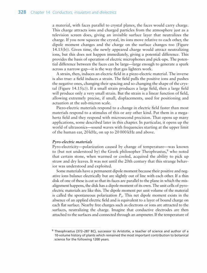
a material, with faces parallel to crystal planes, the faces would carry charge.This charge attracts ions and charged particles from the atmosphere just as atelevision screen does, giving an invisible surface layer that neutralizes thecharge. If you now squeeze the crystal, its ions move relative to each other, thedipole moment changes and the charge on the surface changes too (Figure14.15(b)). Given time, the newly appeared charge would attract neutralizingions, but this does not happen immediately, giving a potential difference. Thisprovides the basis of operation of electric microphones and pick-ups. The poten-tial difference between the faces can be large—large enough to generate a sparkacross a narrow gap—it is the way that gas lighters work.
A strain, then, induces an electric field in a piezo-electric material. The inverseis also true: a field induces a strain. The field pulls the positive ions and pushesthe negative ones, changing their spacing and so changing the shape of the crys-tal (Figure 14.15(c)). If a small strain produces a large field, then a large fieldwill produce only a very small strain. But the strain is a linear function of field,allowing extremely precise, if small, displacements, used for positioning andactuation at the sub-micron scale.
Piezo-electric materials respond to a change in electric field faster than mostmaterials respond to a stimulus of this or any other kind. Put them in a mega-hertz field and they respond with microsecond precision. That opens up manyapplications, some described later in this chapter. In particular, it opens up theworld of ultrasonics—sound waves with frequencies starting at the upper limitof the human ear, 20 kHz, on up to 20 000 kHz and above.
Pyro-electric materialsPyro-electricity—polarization caused by change of temperature—was knownto (but not understood by) the Greek philosopher Theophrastus,8 who notedthat certain stone, when warmed or cooled, acquired the ability to pick upstraw and dry leaves. It was not until the 20th century that this strange behav-ior was understood and exploited.
Some materials have a permanent dipole moment because their positive and neg-ative ions balance electrically but are slightly out of line with each other. If a thindisk of one of these is cut so that its faces are parallel to the plane in which the mis-alignment happens, the disk has a dipole moment of its own. The unit cells of pyro-electric materials are like this. The dipole moment per unit volume of the materialis called the spontaneous polarization Ps. This net dipole moment exists in theabsence of an applied electric field and is equivalent to a layer of bound charge oneach flat surface. Nearby free charges such as electrons or ions are attracted to thesurfaces, neutralizing the charge. Imagine that conductive electrodes are thenattached to the surfaces and connected through an ampmeter. If the temperature of
328 Chapter 14 Conductors, insulators and dielectrics
8 Theophrastus (372–287 BC), successor to Aristotle, a teacher of science and author of a 10-volume history of plants which remained the most important contribution to botanicalscience for the following 1200 years.
Ch14-H8391.qxd 1/16/07 6:10 PM Page 328
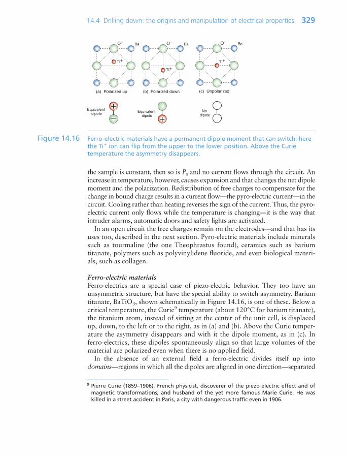
the sample is constant, then so is Ps and no current flows through the circuit. Anincrease in temperature, however, causes expansion and that changes the net dipolemoment and the polarization. Redistribution of free charges to compensate for thechange in bound charge results in a current flow—the pyro-electric current—in thecircuit. Cooling rather than heating reverses the sign of the current. Thus, the pyro-electric current only flows while the temperature is changing—it is the way thatintruder alarms, automatic doors and safety lights are activated.
In an open circuit the free charges remain on the electrodes—and that has itsuses too, described in the next section. Pyro-electric materials include mineralssuch as tourmaline (the one Theophrastus found), ceramics such as bariumtitanate, polymers such as polyvinylidene fluoride, and even biological materi-als, such as collagen.
Ferro-electric materialsFerro-electrics are a special case of piezo-electric behavior. They too have anunsymmetric structure, but have the special ability to switch asymmetry. Bariumtitanate, BaTiO3, shown schematically in Figure 14.16, is one of these. Below acritical temperature, the Curie9 temperature (about 120°C for barium titanate),the titanium atom, instead of sitting at the center of the unit cell, is displacedup, down, to the left or to the right, as in (a) and (b). Above the Curie temper-ature the asymmetry disappears and with it the dipole moment, as in (c). Inferro-electrics, these dipoles spontaneously align so that large volumes of thematerial are polarized even when there is no applied field.
In the absence of an external field a ferro-electric divides itself up intodomains—regions in which all the dipoles are aligned in one direction—separated
14.4 Drilling down: the origins and manipulation of electrical properties 329
Ti+
BaO−
Equivalent dipole
(c) Unpolarized
Ti+
BaO−
Ti+
BaO−
(a) Polarized up (b) Polarized down
+ +
Equivalent
dipoleNo
dipole
Figure 14.16 Ferro-electric materials have a permanent dipole moment that can switch: herethe Ti ion can flip from the upper to the lower position. Above the Curietemperature the asymmetry disappears.
9 Pierre Curie (1859–1906), French physicist, discoverer of the piezo-electric effect and ofmagnetic transformations; and husband of the yet more famous Marie Curie. He waskilled in a street accident in Paris, a city with dangerous traffic even in 1906.
Ch14-H8391.qxd 1/16/07 6:10 PM Page 329

by domain walls at which the direction of polarization changes (Figure 14.17).The domains orient themselves so that the dipole moment of one more or less can-cels those of its neighbors. If a field is applied the domain walls move so that thosepolarized parallel to the field grow and those polarized across or against it shrink,until the entire sample is polarized (or ‘poled’) in just one direction. Figure 14.18shows how the polarization P changes as the field E is increased: P increases,reaching a maximum at the saturation polarization, Ps. If the field is now removed,a large part of the polarization remains (the remanent polarization), which is onlyremoved by reversing the field to the value Ec, the coercive field. The figureshows a complete cycle through full reverse polarization, ending up again with fullforward poling. The little inserts show the domain structures round the cycle.
330 Chapter 14 Conductors, insulators and dielectrics
Applied magnetic field E
and polarization PDomain wall
Domainof dipoles
No applied fieldno net polarization
Figure 14.17 Ferro-electric domains arrange themselves so that their dipole moments cancel.In an electric field E they align, giving the crystal a net dipole moment, whichcan be large.
Electric field E
Polarization P
Saturation polarization
Coercive field Ec
Remanentpolarization
Coercive field −Ec
Figure 14.18 A ferro-electric hysteresis curve.
Ch14-H8391.qxd 1/16/07 6:10 PM Page 330
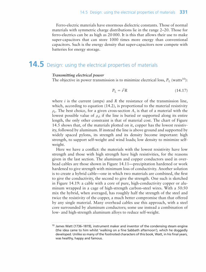
Ferro-electric materials have enormous dielectric constants. Those of normalmaterials with symmetric charge distributions lie in the range 2–20. Those forferro-electrics can be as high as 20 000. It is this that allows their use to makesuper-capacitors that can store 1000 times more energy than conventionalcapacitors. Such is the energy density that super-capacitors now compete withbatteries for energy storage.
14.5 Design: using the electrical properties of materials
Transmitting electrical powerThe objective in power transmission is to minimize electrical loss, PL (watts10):
PL i2R (14.17)
where i is the current (amps) and R the resistance of the transmission line,which, according to equation (14.2), is proportional to the material resistivityρe. The best choice, for a given cross-section A, is that of a material with thelowest possible value of ρe; if the line is buried or supported along its entirelength, the only other constraint is that of material cost. The chart of Figure14.5 shows that, of the materials plotted on it, copper has the lowest resistiv-ity, followed by aluminum. If instead the line is above ground and supported bywidely spaced pylons, its strength and its density become important: highstrength, to support self-weight and wind loads; low density to minimize self-weight.
Here we have a conflict: the materials with the lowest resistivity have lowstrength and those with high strength have high resistivities, for the reasonsgiven in the last section. The aluminum and copper conductors used in over-head cables are those shown in Figure 14.11—precipitation hardened or workhardened to give strength with minimum loss of conductivity. Another solutionis to create a hybrid cable—one in which two materials are combined, the firstto give the conductivity, the second to give the strength. One such is sketchedin Figure 14.19: a cable with a core of pure, high-conductivity copper or alu-minum wrapped in a cage of high-strength carbon–steel wires. With a 50:50mix the hybrid, when averaged, has roughly half the strength of the steel andtwice the resistivity of the copper, a much better compromise than that offeredby any single material. Many overhead cables use this approach, with a steelcore surrounded by aluminum conductors; some use instead a combination oflow- and high-strength aluminum alloys to reduce self-weight.
14.5 Design: using the electrical properties of materials 331
10 James Watt (1736–1819), instrument maker and inventor of the condensing steam engine(the idea came to him whilst ‘walking on a fine Sabbath afternoon‘), which he doggedlydeveloped. Unlike so many of the footnoted characters of this book, Watt, in his final years,was healthy, happy and famous.
Ch14-H8391.qxd 1/16/07 6:10 PM Page 331

Electrical insulationElectrical insulators keep electricity where it is supposed to be. The charts ofFigures 14.6 and 14.7 show that most polymers are excellent electrical insulators,with resistivities above 1020µΩ.cm. They are used for cable insulation, for casingsof plugs, connectors and switchgear. Many ceramics, too, are good electricalinsulators, notably alumina (Al2O3), silica (SiO2) and glass (Pyrex); they are usedin applications in which rigidity and resistance to heat are important, such as sub-strates for electronic circuits and high-voltage insulators. Where electrical isola-tion is vital, the objective is to maximize resistivity, but as with conduction thereare usually additional constraints. Here is an example.
The electric plug (Figure 14.20) is perhaps the commonest of electrical prod-ucts. It has a number of components, most performing more than one function.
332 Chapter 14 Conductors, insulators and dielectrics
Copper
Steel
Outercasing
Figure 14.19 A hybrid cable made up of strands of copper reinforced with strands of steel.
Figure 14.20 An electric plug. The casing must be an insulator, be moldable and havesufficient strength to tolerate working loads.
Ch14-H8391.qxd 1/16/07 6:10 PM Page 332

The most obvious are the casing and the pins, though there are many more(connectors, a cable clamp, fasteners and, in some plugs, a fuse). Power plugshave two or three pins and are of robust construction. System plugs, like thatof the video port of a computer, have 25 or more pins and are miniaturized anddelicate, placing more importance on the mechanical as well as the electricalproperties of the materials of the pins and casing. The task here is to select amaterial for the casing of the plug.
The shape is complicated, the part will be made in very large numbers and pinshave to be molded in. The only practical way to make it is by using a polymer.The designers set a required strength of at least 25 MPa and, of course, the elec-trical resistivity should be as high as possible. The chart of Figure 14.6 suggestsABS, PMMA and PC as suitable candidates—they are strong enough and havehigh resistivity. But there is a problem: all three are thermoplastics; they soften ifthey get hot. If circuit overload or poor contact generates heat, the plug willsoften, distort and even melt, presenting hazards. So the choice has to be a ther-moset, which will char rather than melt. The chart suggests Phenolic—and that iswhat plugs are really made of. The CES software allows much more sophisticatedsuggestions: try the Exercises at the end of this chapter to refine the choice.
Electrical insulation with thermal conduction: keeping microchips coolAs microchips shrink in scale and clock speeds rise, overheating becomes aproblem. The Pentium chip of today’s PCs already reaches 85°C, requiringforced cooling. Multiple-chip modules (MCMs) pack as many as 130 chips onto a single substrate, and there the problem is more severe. Heating is keptunder control by attaching the chips to a heat sink (Figure 14.21), taking carethat they are in good thermal contact. The heat sink now becomes a criticalcomponent, limiting further development of the electronics.
To drain heat away from the chips as fast as possible, the heat sink must havethe highest possible thermal conductivity, λ. Metals like copper and aluminumhave high λ, but they are good electrical conductors and this is bad because itallows electrical coupling and stray capacitance between chip and heat sink,slowing the information transfer rate (remember the time delay in a circuit isτ RC). To prevent this, the heat sink must be an excellent electrical insulator.
Figure 14.5 is the chart with the properties we want: thermal conductivity λand electrical resistivity ρe. The materials at the top right have high thermal
14.5 Design: using the electrical properties of materials 333
Connecting pinsSubstrate
Chips
Cooling fins
Heatsink
Figure 14.21 A heat sink. It must conduct heat but not electricity.
Ch14-H8391.qxd 1/16/07 6:10 PM Page 333

conductivity and very high resistivity—they are electrical insulators. The bestchoice of material for the heat sink, then, is aluminum nitride (AlN), alumina(Al2O3) or silicon carbide (SiC). It is these that are used for such heat sinks.
Using dielectric loss: microwave heatingWhen you cook a chicken in a microwave oven, you are using dielectric loss.Looking back at equation (14.13) we see that the dielectric loss, and thus theheating, is proportional to the loss factor L εr tan δ, one axis of the chart ofFigure 14.7. Chickens do not appear on the chart, but they do have a high lossfactor, as do all foods that contain water. There are other ways of cookingchicken, but this one has the advantage that it is quick because microwavesabsorb uniformly through the section, giving uniform heating. Microwaveheating is not just useful in the kitchen; it is also widely used for industrial heat-ing. Wood can be dried, adhesives cured, polymers molded and ceramics sin-tered using microwave heating. As equation (14.13) implies, the higher thefrequency f of the electric field, the greater the heating, so it is common, in theindustrial application of microwaves, to use gigahertz frequencies (0.3–3 GHz).
Using dielectric loss: stealth technologyRadar, developed during the Second World War, played a major role in protect-ing Britain (and others) from air attack. It works by transmitting bursts ofradio-frequency waves that are reflected back by objects in their path. Theradar antenna measures the time it takes for the reflection to arrive back, fromwhich the distance and speed of the object are computed.
The metal body of an aircraft is an excellent radar reflector and its curvedshape causes it to reflect in all directions—just what is needed for safe air-traf-fic control. But if your aim is to avoid detection, reflection is the last thing youwant. Stealth technology combines three tricks to minimize it:
• A shape made up of flat planes that reflect the radar signal away from thedetector unless it lies exactly normal to the surface.
• Non-metallic structural materials—usually composites—that are semi-transparent to microwaves (see Chapter 16 for how to achieve transparency).
• Surface coatings of radar-absorbing materials (called RAMs) that absorbmicrowaves rather than reflecting them. RAMs use dielectric loss. A surfacelayer of a material with a large value of loss factor εr tan δ, a ferro-electricfor example, attenuates the incoming wave, diminishing the reflected signal.
Avoiding dielectric loss: materials for radomesThe function of a radome is to shield a microwave antenna from the adverseeffects of wind and weather while having as little effect as possible on the sig-nal it sends and receives (Figure 14.22). When trying to detect incoming signalsthat are weak to begin with, even a small attenuation of the signal as it passesthrough the radome decreases the sensitivity of the system. Yet the radomemust withstand structural loads, loads caused by pressure difference betweenthe inside and outside of the dome, and—in the case of supersonic flight—high
334 Chapter 14 Conductors, insulators and dielectrics
Ch14-H8391.qxd 1/16/07 6:10 PM Page 334

temperatures. So the problem here is the opposite of stealth coatings; it is howto design materials that do not attenuate electromagnetic waves. The answer isto seek those with exceptionally low values of εr tan δ. And since the radomecarries structural loads, they should also be strong.
The chart of Figure 14.7 shows that some polymers have low loss factor, butthey are not very strong. Reinforcing them with glass fibers, creating GFRPs,combines low loss with good strength. When, additionally, high temperaturesare involved, the ceramics that appear on the upper left of Figure 14.7—silica(SiO2), alumina (Al2O3) and silicon nitride (Si3N4)—are employed.
Piezo-electric actuation: ink-jet printersInk-jet printing is now widely used to make black and white or color prints.Many printers use thermal (‘bubble-jet’) technology, in which a tiny heatingwire boils a minute volume of ink in the print-head, creating a vapor bubble.The sudden pressure this creates ejects a droplet to ink. The bubble collapses asthe wire cools, sucking more ink from a reservoir into the print-head to replacethat in the droplet. Very simple, but thermal technology gives little control of the droplet size or shape.
The alternative is the piezo print-head, one unit of which is sketched in Figure14.23. An electric field applied to the disk of piezo-electric material transmits akick to the vibration plate, creating a pressure pulse that spits a droplet of ink fromthe nozzle. On relaxation, more ink is drawn in to replace it. Like bubble-jet print-ers, piezo print-heads have 300–600 nozzles. The great advantage of piezo tech-nology is the control of the shape and duration of the pulse delivered by the piezodisk. The droplets of ink are significantly smaller, and the control of droplet sizegives greater resolution and color gradation.
Pyro-electric thermal imagingNight vision, the location of survivors in disaster areas, the filming of wildlife andmuch else make use of thermal imaging. The technology is comparatively new—the
14.5 Design: using the electrical properties of materials 335
2 R
t
∆p
Radome
Figure 14.22 A radome. The shell must be transparent to microwaves, requiring a lowdielectric loss factor with high strength.
Ch14-H8391.qxd 1/16/07 6:10 PM Page 335
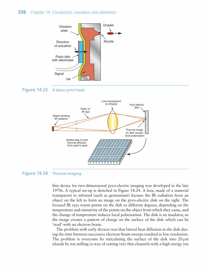
first device for two-dimensional pyro-electric imaging was developed in the late1970s. A typical set-up is sketched in Figure 14.24. A lens, made of a materialtransparent to infrared (such as germanium) focuses the IR radiation from anobject on the left to form an image on the pyro-electric disk on the right. Thefocused IR rays warm points on the disk to different degrees, depending on thetemperature and emissivity of the points on the object from which they came, andthe change of temperature induces local polarization. The disk is an insulator, sothe image creates a pattern of charge on the surface of the disk which can be‘read’ with an electron beam.
The problem with early devices was that lateral heat diffusion in the disk dur-ing the time between successive electron-beam sweeps resulted in low resolution.The problem is overcome by reticulating the surface of the disk into 20 µmislands by ion milling (a way of cutting very thin channels with a high energy ion
336 Chapter 14 Conductors, insulators and dielectrics
Ink
Piezo diskwith electrodes
Vibration plate
Droplet
Nozzle Directionof actuation
Signal
Figure 14.23 A piezo print-head.
Pyro-electricdisk
Lens transparentto infrared
Slotted disk to limit thermal diffusion from pixel to pixel
Object emittingIR radiation
Thermal imageon disk causes
local polarization
Paths of IR rays
Figure 14.24 Thermal imaging.
Ch14-H8391.qxd 1/16/07 6:10 PM Page 336
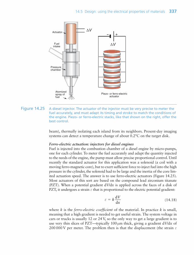
beam), thermally isolating each island from its neighbors. Present-day imagingsystems can detect a temperature change of about 0.2°C on the target disk.
Ferro-electric actuation: injectors for diesel enginesFuel is injected into the combustion chamber of a diesel engine by micro-pumps,one for each cylinder. To meter the fuel accurately and adapt the quantity injectedto the needs of the engine, the pump must allow precise proportional control. Untilrecently the standard actuator for this application was a solenoid (a coil with amoving ferro-magnetic core), but to exert sufficient force to inject fuel into the highpressure in the cylinder, the solenoid had to be large and the inertia of the core lim-ited actuation speed. The answer is to use ferro-electric actuators (Figure 14.25).Most actuators of this sort are based on the compound lead zirconium titanate(PZT). When a potential gradient dV/dx is applied across the faces of a disk ofPZT, it undergoes a strain ε that is proportional to the electric potential gradient:
(14.18)
where k is the ferro-electric coefficient of the material. In practice k is small,meaning that a high gradient is needed to get useful strain. The system voltage incars or trucks is usually 12 or 24 V, so the only way to get a large gradient is touse very thin slices of PZT—typically 100 µm thick, giving a gradient dV/dx of200 000 V per meter. The problem then is that the displacement (the strain ε
ε kVx
dd
14.5 Design: using the electrical properties of materials 337
∆V
+
Piezo- or ferro-electricactuator
∆V
Fuelintake
Actuator
Pressurechamber
Atomizedspray offuel
Figure 14.25 A diesel injector. The actuator of the injector must be very precise to meter thefuel accurately, and must adapt its timing and stroke to match the conditions ofthe engine. Piezo- or ferro-electric stacks, like that shown on the right, offer thebest control.
Ch14-H8391.qxd 1/16/07 6:10 PM Page 337
times the thickness of the disk, x) is small. The solution is to make a stack likethat shown, expanded, on the right of Figure 14.25. The thin (x 100 µm) slicesof PZT are sandwiched between conducting electrodes, alternately charged,creating the gradient. A stack of 100 (still only 10 mm high) gives adequate dis-placements. These actuators are half the size and allow twice the pulse rate ofsolenoids, giving more precise control, performance and fuel economy.
14.6 Summary and conclusions
All materials contain charged particles: electrons, protons, ions, charged mole-cules and the like. An electric field E exerts a force qE on a charge q, pushing itin the direction of the field if q is positive and in the opposite direction if it isnegative. If the particles can move freely, as electrons can in metals, an electriccurrent flows through the material, which we refer to as conduction. If, instead,they cannot move freely, as is the case in insulators, the particles are still dis-placed slightly by the field, leading to dielectric polarization.
Materials that polarize easily have a high dielectric constant. If used as the insu-lating film of a capacitor, the polarization screens the electrodes from each other,increasing the capacitance. The slight displacement of charge has other conse-quences. One of these is electrostriction: the charge movement causes the materialto change shape slightly. If the material is made up of ions and these are arrangedin a way that lacks a center of symmetry, a further effect appears: that of piezo-elec-tric response. The lack of symmetry means that each molecule carries a dipolemoment, and within a single crystal these are aligned. An electric field causes achange of shape and a change of shape changes the molecular dipole moment, thusinducing a change in polarization, generating a field. A change of temperature, too,changes the molecular dipole moment, so materials that are piezo-electric are alsopyro-electric. A few materials have a further property: that of molecular asymme-try that can switch direction because ions can occupy one of several equivalent sitesin the crystal. These materials are ferro-electric; the molecular dipoles sponta-neously align to form polarized domains. In the relaxed state the domains take uporientations such that the field of one is canceled by those of its neighbors, butwhen ‘poled’ by placing it in an electric field, the domains align, giving a large netpolarization that is retained when the field is removed.
All these effects have practical utility, examples of which are described in thechapter.
14.7 Further reading
Braithwaite, N. and Weaver, G. (1990) Electronic Materials, The Open University andButterworth-Heinemann, Oxford, UK. ISBN 0-408-02840-8. (One of the excellentOpen University texts that form part of their Materials program.)
Jiles, D. (2001) Introduction to the Electronic Properties of Materials, 2nd edition,Nelson Thornes, Cheltenham, UK. ISBN 0-7487-6042-3. (The author develops the
338 Chapter 14 Conductors, insulators and dielectrics
Ch14-H8391.qxd 1/16/07 6:10 PM Page 338

electronic properties of materials, relating them to thermal and optical as well as theelectrical behavior.)
Solymar, L. and Walsh, D. (2004) Electrical Properties of Materials, 7th edition, OxfordUniversity Press, Oxford, UK. ISBN 0-19-926793-6. (A mature introduction to elec-trical materials.)
14.8 Exercises
14.8 Exercises 339
Exercise E14.1 Why do metals conduct electricity? Why do insulators not conduct electric-ity, at least when cold?
Exercise E14.2 What is a dielectric? What are its important dielectric properties? What ismeant by polarization? Why do some dielectrics absorb microwave radiationmore than others?
Exercise E14.3 It is much easier to measure the electrical conductivity of a material than tomeasure its thermal conductivity. Use the Weidemann–Franz law Section14.3 to find the thermal conductivities of:(a) An alloy that has an electrical resistivity ρe of 28 µΩ.cm.(b) Tungsten of the kind used for lamp filaments that has an electrical con-
ductivity κe of 9.9 106S/m (1 S/m is 1/Ω.m).
Exercise E14.4 The metal zinc has free electron concentration per unit volume, nv, of1.3 1029/m3 and an electron mobility µe of 8 104m2/V.s. The chargecarried by an electron, e, is 1.6 1019 coulomb. Based on this information,what is the electrical conductivity of zinc? Handbooks list the measuredresistivity of zinc as 5.9 µΩ.cm. Is this consistent with your calculation?(Watch the units.)
Exercise E14.5 A power line is to carry 5 kA at 11 kV using pylons 460 m apart. The dip din a wire of weight ml per unit length strung between pylons L apart at a ten-sion T is given by d L2ml/8T. The maximum tension allowed is 0.8 of theyield stress, σy. If the maximum allowable dip is 6 m, which of the materialsin the table could be used?
Exercise E14.6 A material is required for a transmission line that gives the lowest full-lifecost over a 20-year period. The total cost is the sum of the material cost and
Material Electrical resistivity, Yield stress, Density, ρe (Ωm) σy (MPa) ρ (kg/m3)
Aluminum 1.7 108 102 2700Copper 1.5 108 300 8900Carbon steel 55 108 510 7800
Ch14-H8391.qxd 1/16/07 6:10 PM Page 339

340 Chapter 14 Conductors, insulators and dielectrics
the cost of the energy dissipated in joules. The cost of electricity CE is6 103$/MJ. Material prices are listed in the table. Derive an expressionfor the total cost per meter of cable in terms of the cross-sectional area A(which is a free parameter), the material and electrical costs and the materialparameters. Show that the minimum cost occurs when the two contributionsto the cost are equal. Hence derive a performance index for the material anddecide on the best of the materials in the table.
Exercise E14.7 In the discussion of conductors, a 50:50 mix of copper and steel strands wassuggested for transmission cables. Using the values in the table for resistivityand strength, calculate the effective values of both for the cable, assuming arule of mixtures. Plot this on copies of the σy – ρe chart of Figures 14.6 and14.11 to explore its performance.
Low density, we said, was important for long-span transmission linesbecause the self-weight becomes significant. Suppose you were asked todesign a hybrid power transmission cable with the lowest possible weight,what combination of materials would you choose? Use information from thecharts for inspiration.
Exercise E14.8 Roughly 50% of all cork that is harvested in Portugal ends up as cork dust, aworthless by-product. As a materials expert, you are approached by an entre-preneur who has the idea of making useful products out of cork dust by com-pacting it and heating it, using microwave heating. The loss factor L of cork is0.21. The entrepreneur reckons he needs a power density P of at least 2 kW perm3 for the process to be economic. If the maximum field E is limited to 102V/m,what frequency f of microwaves will be needed?
Material Strength, Resistivity, σy (MPa) ρe (µΩ.cm)
High-strength steel, cold drawn 1700 22High-conductivity copper, cold drawn 300 1.7
Material Electrical resistivity, Density, Price, ρe (Ωm) ρ (kg/m3) Cm ($/kg)
Aluminum 1.7 108 2700 1.6Copper 1.5 108 8900 5.2Steel 55 108 7800 0.5
Ch14-H8391.qxd 1/16/07 6:10 PM Page 340

14.9 Exploring design with CES (use Level 2 unless stated otherwise)
14.9 Exploring design with CES 341
Exercise E14.9 Use the ‘Search’ facility of CES to search for:
(a) Electrical conductors.(b) Heat sinks.
Exercise E14.10 The analysis of heat sinks in Chapter 3 formulated the following design con-straints and objective. They are summarized in the table. Use the selector tofind the material that best meets them.
Exercise E14.11 The sheath of the cable shown in Figure 14.19 is molded over the bundledwires. The material of the sheath must be electrically insulating, flexible,water resistant and cheap. The table translates the requirements. Apply theconstraints using a ‘Tree’ and a ‘Limit’ stage, then plot a bar chart of mate-rial price to find the three least expensive materials that meet all the constraints.
Exercise E14.12 The pins of the plug of Figure 14.20 must conduct electricity well, be corro-sion resistant so that contact remains good, and be hard enough to resistabrasion and wear. The table translates the requirements. Apply these andrank the promising candidates by material price.
Function • Cable sheathing
Constraints • Able to be molded• Good electrical insulator• Durability in fresh water: very good• Young’s modulus 3 GPa
Objective • Minimize material price
Free variable • Choice of material
Function • Heat sink
Constraints • Material must be good electrical insulator• Maximum operating temperature 200°C
Objective • Maximize thermal conductivity
Free variable • Choice of material
Ch14-H8391.qxd 1/16/07 6:10 PM Page 341

342 Chapter 14 Conductors, insulators and dielectrics
Exercise E14.13 The casing of the plug of Figure 14.20 performs both a mechanical and anelectrical function. It must insulate, and it must also be rigid and resilientenough to tolerate service loads. (Resilient means it must be capable of someelastic distortion requiring a high yield strain, σy/E).
Function • Plug casing
Constraints • Able to be molded• Good electrical insulator• Flammability: non-flammable or
self-extinguishing• Young’s modulus 2 GPa• Yield strain σy/E 0.01
Objective • Minimize material price
Free variable • Choice of material
Function • Connecting pins for power plug
Constraints • Good electrical insulator• Durability in fresh water: very good• Hardness 200 HV
Objective • Minimize material price
Free variable • Choice of material
Ch14-H8391.qxd 1/16/07 6:10 PM Page 342

14.10 Exploring the science with CES Elements
14.10 Exploring the science with CES Elements 343
Exercise E14.14 Make a chart with Atomic number on the x-axis (use a linear scale) andElectrical conductivity κ on the y-axis. Convert the values of resistivity ρe (whichare in units of µΩ.cm in the database) to those of conductivity in siemens/m(S/m); use κ 108/ρe. This can be made using the ‘Advanced’ facility in the axis-choice dialog box. Does conductivity vary in a periodic way across thePeriodic Table? Which three elements have the highest conductivities?
Exercise E14.15 Explore the Wiedemann–Franz relation for the elements. To do so, make achart of electrical conductivity, constructed as in the previous example, onthe x-axis and thermal conductivity on the y-axis. Limit the selection to met-als only by using a ‘Limit’ stage—State at 300 K. Fit an equation to theresulting plot. If you were now given a new alloy with an electrical conduc-tivity of 4 107S/m, what would you estimate its thermal conductivity to be?(Relations such as this one provide ways of building ‘intelligent checking’ ofdata into material property databases.)
Exercise E14.16 Make a chart with atomic number on the x-axis (use a linear scale) anddielectric constant on the y-axis. Do you see any general trend? If so, howwould you explain it?
Exercise E14.17 It is proposed to use the temperature dependence of electrical resistivity forsensing. Plot this quantity against relative cost to identify three cheap metalswith high values of this temperature dependence.
Exercise E14.18 Equation (14.15) of the text derives the electrical conductivity as
κe nv e µe
The CES Elements database contains data for the free electron concentrationnv and the electron mobility µe. You will find the electronic charge under‘Constants/Parameters’ in the ‘Advanced’ facility for choosing the axes ofthe chart. Make a chart using the ‘Advanced’ facility with κe nv e µe on they-axis and the reciprocal of the resistivity on the x-axis. Make sure you havemade all the units self-consistent. How well does this equation describes themeasured conductivities of metals?
Exercise E14.19 Explore superconductivity across the Periodic Table. Use CES Elements toplot superconducting transition temperature, Tc, against the atomic number(use linear scales). Which element has the highest transition temperature?What is Tc for this element?
Ch14-H8391.qxd 1/16/07 6:10 PM Page 343

This page intentionally left blank

Chapter 15Magnetic materials
Chapter contents
15.1 Introduction and synopsis 34615.2 Magnetic properties: definition
and measurement 34615.3 Charts for magnetic properties 35115.4 Drilling down: the physics and
manipulation of magnetic properties 35315.5 Materials selection for
magnetic design 35815.6 Summary and conclusions 36315.7 Further reading 36315.8 Exercises 36415.9 Exploring design with CES 36515.10 Exploring the science with CES
Elements 366
Magnet materials in action. The audio-frequencytransformer on the left has a soft magnetic core. The
DC motor on the right has a hard (permanent)magnetic stator and a soft magnetic rotor
Ch15-H8391 1/16/07 6:42 PM Page 345
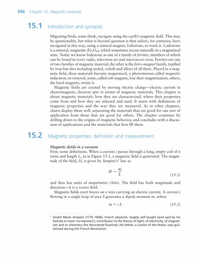
346 Chapter 15 Magnetic materials
15.1 Introduction and synopsis
Migrating birds, some think, navigate using the earth’s magnetic field. This maybe questionable, but what is beyond question is that sailors, for centuries, havenavigated in this way, using a natural magnet, lodestone, to track it. Lodestoneis a mineral, magnetite (Fe3O4), which sometimes occurs naturally in a magnetizedstate. Today we know lodestone as one of a family of ferrites, members of whichcan be found in every radio, television set and microwave oven. Ferrites are oneof two families of magnetic material; the other is the ferro-magnet family, typifiedby iron but also including nickel, cobalt and alloys of all three. Placed in a mag-netic field, these materials become magnetized, a phenomenon called magneticinduction; on removal, some, called soft magnets, lose their magnetization, others,the hard magnets, retain it.
Magnetic fields are created by moving electric charge—electric current inelectromagnets, electron spin in atoms of magnetic materials. This chapter isabout magnetic materials: how they are characterized, where their propertiescome from and how they are selected and used. It starts with definitions ofmagnetic properties and the way they are measured. As in other chapters,charts display them well, separating the materials that are good for one sort ofapplication from those that are good for others. The chapter continues bydrilling down to the origins of magnetic behavior, and concludes with a discus-sion of applications and the materials that best fill them.
15.2 Magnetic properties: definition and measurement
Magnetic fields in a vacuumFirst, some definitions. When a current i passes through a long, empty coil of nturns and length L, as in Figure 15.1, a magnetic field is generated. The magni-tude of the field, H, is given by Ampère’s1 law as
(15.1)
and thus has units of amps/meter (A/m). The field has both magnitude anddirection—it is a vector field.
Magnetic fields exert forces on a wire carrying an electric current. A current iflowing in a single loop of area S generates a dipole moment m, where
m i S (15.2)
HniL
1 André Marie Ampère (1775–1836), French physicist, largely self-taught (and said by hisfiancée to have ‘no manners’), contributor to the theory of light, of electricity, of magnet-ism and to chemistry (he discovered fluorine). His father, a Justice of the Peace, was guil-lotined during the French Revolution.
Ch15-H8391 1/16/07 6:42 PM Page 346
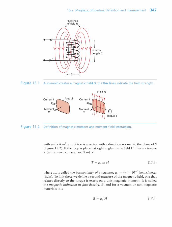
15.2 Magnetic properties: definition and measurement 347
with units A.m2, and it too is a vector with a direction normal to the plane of S(Figure 15.2). If the loop is placed at right angles to the field H it feels a torqueT (units: newton.meter, or N.m) of
T µo m H (15.3)
where µo is called the permeability of a vacuum, µo 4π 107 henry/meter(H/m). To link these we define a second measure of the magnetic field, one thatrelates directly to the torque it exerts on a unit magnetic moment. It is calledthe magnetic induction or flux density, B, and for a vacuum or non-magneticmaterials it is
B µo H (15.4)
i
i
n turnsLength L
Flux lines of field H
2r
Figure 15.1 A solenoid creates a magnetic field H; the flux lines indicate the field strength.
Area S
Momentm
Current i
Torque T
Momentm
Current i
Field H
Figure 15.2 Definition of magnetic moment and moment-field interaction.
Ch15-H8391 1/16/07 6:42 PM Page 347

Its units are tesla2, so 1 tesla is 1 HA/m2. A magnetic induction B of 1 teslaexerts a torque of 1 N.m on a unit dipole at right angles to the field H.
Magnetic fields in materialsIf the space inside the coil of Figure 15.2 is filled with a material, as in Figure15.3, the induction within it changes. This is because its atoms respond to thefield by forming little magnetic dipoles in ways that are explained in Section 15.4.The material acquires a macroscopic dipole moment or magnetization, M (itsunits are A/m, like H). The induction becomes
B µo (H M) (15.5)
The simplicity of this equation is misleading, since it suggests that M and H areindependent; in reality M is the response of the material to H, so the two arecoupled. If the material of the core is ferro-magnetic, the response is a very strongone and it is nonlinear, as we shall see in a moment. It is usual to rewrite equation(15.5) in the form
B µR µo H
where µR is called the relative permeability, and like the relative permittivity(the dielectric constant) of Chapter 14, it is dimensionless. The magnetization,M, is thus
M (µR 1) H χ H (15.6)
348 Chapter 15 Magnetic materials
i
i
Flux linesof inductance B
Magneticmaterial
Figure 15.3 A magnetic material exposed to a field H becomes magnetized, concentratingthe flux lines.
2 Nikola Tesla (1856–1943), Serbian-American inventor, discoverer of rotating magneticfields, the basis of most alternating current machinery, inventor of the Tesla coil and of arudimentary flying machine (never built).
Ch15-H8391 1/16/07 6:42 PM Page 348
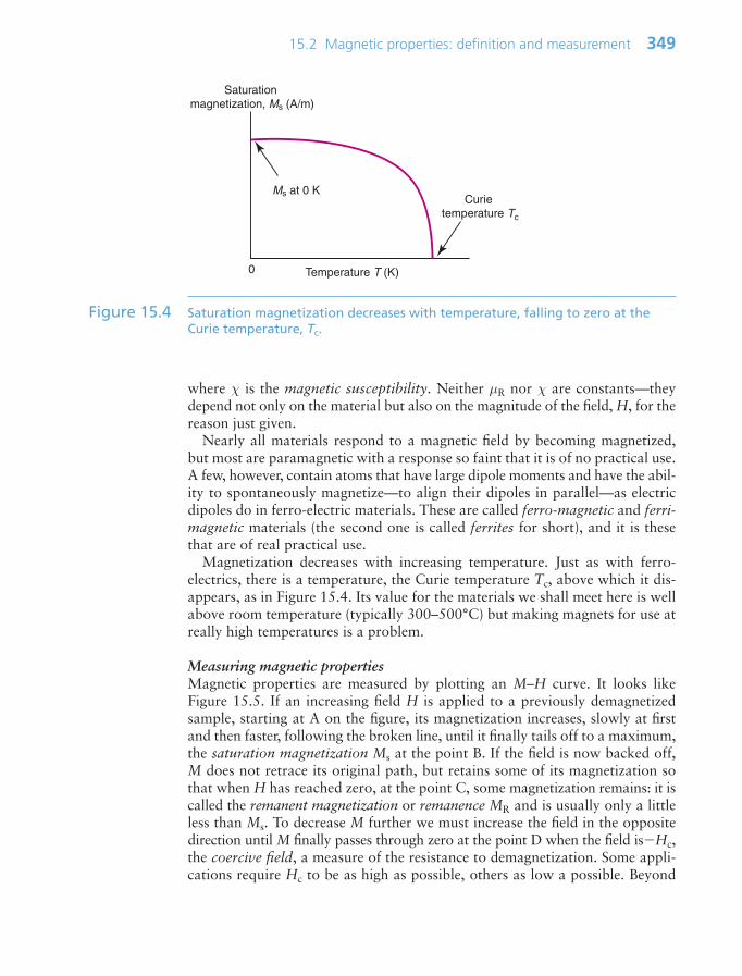
where χ is the magnetic susceptibility. Neither µR nor χ are constants—theydepend not only on the material but also on the magnitude of the field, H, for thereason just given.
Nearly all materials respond to a magnetic field by becoming magnetized,but most are paramagnetic with a response so faint that it is of no practical use.A few, however, contain atoms that have large dipole moments and have the abil-ity to spontaneously magnetize—to align their dipoles in parallel—as electricdipoles do in ferro-electric materials. These are called ferro-magnetic and ferri-magnetic materials (the second one is called ferrites for short), and it is thesethat are of real practical use.
Magnetization decreases with increasing temperature. Just as with ferro-electrics, there is a temperature, the Curie temperature Tc, above which it dis-appears, as in Figure 15.4. Its value for the materials we shall meet here is wellabove room temperature (typically 300–500°C) but making magnets for use atreally high temperatures is a problem.
Measuring magnetic propertiesMagnetic properties are measured by plotting an M–H curve. It looks likeFigure 15.5. If an increasing field H is applied to a previously demagnetizedsample, starting at A on the figure, its magnetization increases, slowly at firstand then faster, following the broken line, until it finally tails off to a maximum,the saturation magnetization Ms at the point B. If the field is now backed off,M does not retrace its original path, but retains some of its magnetization sothat when H has reached zero, at the point C, some magnetization remains: it iscalled the remanent magnetization or remanence MR and is usually only a littleless than Ms. To decrease M further we must increase the field in the oppositedirection until M finally passes through zero at the point D when the field isHc,the coercive field, a measure of the resistance to demagnetization. Some appli-cations require Hc to be as high as possible, others as low a possible. Beyond
15.2 Magnetic properties: definition and measurement 349
Saturation magnetization, Ms (A/m)
Temperature T (K)
Curie temperature Tc
Ms at 0 K
0
Figure 15.4 Saturation magnetization decreases with temperature, falling to zero at theCurie temperature, Tc.
Ch15-H8391 1/16/07 6:42 PM Page 349

point D the magnetization M starts to increase in the opposite direction, eventu-ally reaching saturation again at the point E. If the field is now decreased again,M follows the curve through F and G back to full forward magnetic saturationagain at B to form a closed M–H circuit called the hysteresis loop.
Magnetic materials are characterized by the size and shape of their hysteresisloops. The initial segment AB is called the initial magnetization curve and its aver-age slope (or sometimes its steepest slope) is the magnetic susceptibility, χ. Theother key properties—the saturation magnetization Ms, the remanence MR andthe coercive field Hc—have already been defined. Each full cycle of the hysteresisloop dissipates an energy per unit volume equal to the area of the loop multipliedby µo, the permeability of a vacuum. This energy appears as heat (it is like magneticfriction). Many texts plot not the M–H curve, but the curve of inductance Bagainst H. Equation (15.5) says that B is proportional to (M H), and the valueof M for any magnetic materials worthy of the name is very much larger thanthe H applied to it, so B µoM and the B–H curve of a ferro-magnetic materiallooks very like its M–H curve (it’s just that the M-axis has been scaled by µo).
There are several ways to measure the hysteresis curve, one of which issketched in Figure 15.6. Here the material forms the core of what is, in effect, atransformer. The oscillating current through the primary input coil creates a fieldH that induces magnetization M in the material of the core, driving it round itshysteresis loop. The secondary coil picks up the inductance, from which theinstantaneous state of the magnetization can be calculated, mapping out the loop.
Magnetic materials differ greatly in the shape and area of their hysteresisloop, the greatest difference being that between soft magnets, which have thin
350 Chapter 15 Magnetic materials
Magnetic field H
Magnetization M
Saturation magnetization, Ms
Coercive field Hc
Remanentmagnetization, MR
Coercive field −Hc
A
BC
D
EF
G
Saturation magnetization, −Ms
Figure 15.5 A hysteresis curve, showing the important magnetic properties.
Ch15-H8391 1/16/07 6:42 PM Page 350
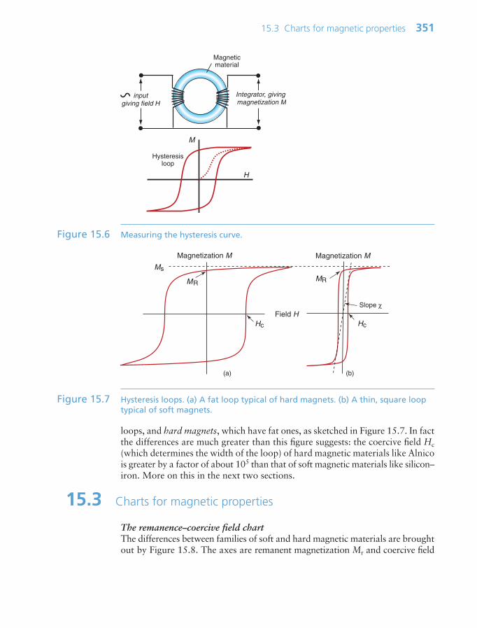
loops, and hard magnets, which have fat ones, as sketched in Figure 15.7. In factthe differences are much greater than this figure suggests: the coercive field Hc(which determines the width of the loop) of hard magnetic materials like Alnicois greater by a factor of about 105 than that of soft magnetic materials like silicon–iron. More on this in the next two sections.
15.3 Charts for magnetic properties
The remanence–coercive field chartThe differences between families of soft and hard magnetic materials are broughtout by Figure 15.8. The axes are remanent magnetization Mr and coercive field
15.3 Charts for magnetic properties 351
H
inputgiving field H
M
Integrator, giving magnetization M
Hysteresisloop
Magneticmaterial
Figure 15.6 Measuring the hysteresis curve.
Hc
MR
Slope χ
Ms
MR
Magnetization M Magnetization M
(a) (b)
Hc
Field H
Figure 15.7 Hysteresis loops. (a) A fat loop typical of hard magnets. (b) A thin, square looptypical of soft magnets.
Ch15-H8391 1/16/07 6:42 PM Page 351

Hc. The saturation magnetization Ms, more relevant for soft magnets, is onlyslightly larger than Mr, so an Ms–Hc chart looks almost the same as this one.There are 12 district families, each enclosed in a colored envelope. The membersof each family, shown as smaller ellipses, have unhelpful tradenames (such as‘H FerriteYBM-1A’) so they are not individually labeled.3 Soft magnets requirehigh Ms and low Hc; they are the ones on the left, with the best near the top. Hardmagnets must hold their magnetism, requiring a high Hc, and to be powerfulthey need a large Mr; they are the ones on the right, with the best again at the top.
In many applications the electrical resistivity is also important because of eddy-current losses, described later. Changing magnetic fields induces eddy currents inconductors but not in insulators. The red and purple ellipses on the chart enclosemetallic ferro-magnetic materials, which are good conductors. The yellow onesdescribe ferrites, which are insulators.
The saturation magnetization–susceptibility chartThis is the chart for selecting soft magnetic materials (Figure 15.9). It shows thesaturation magnetization, Ms—the ultimate degree to which a material can con-centrate magnetic flux—plotted against its susceptibility, χ, which measures theease with which it can be magnetized. Many texts use, instead, the saturationinductance Bs and maximum relative permeability, µR. They are shown on the
352 Chapter 15 Magnetic materials
3 This chart and the next were made with Level 3 of the CES Edu database, which containsdata for 222 magnetic materials. Levels 1 and 2 do not include magnetic materialsbecause of their specialized nature.
Coercive field Hc (A/m)
Rem
anen
t mag
netiz
atio
n M
r (A
/m)
106
105
2x10⁶
2x10⁵
5x10⁵
0.01 0.1 1 10 106105104103102 107
Soft (cubic) ferrites
Hard (hexagonal) ferrites
Metglasamorphous alloys
Permalloys andMuMetal
Permendur
Silicon iron
Neodymium-based alloys
Co–Smalloys
Pt–Coalloys
Alnicos
Fe-Coalloys
Soft iron
Softmagnets
Hardmagnets
2
1
0.5
0.25
0.125
Rem
anen
t ind
uctio
n B
r (T
esla
)
MFA 07
Figure 15.8 Remanent magnetization and coercive force. Soft magnetic materials lie on theleft, hard magnetic materials on the right. The red and purple envelopesenclose electrically conducting materials, the yellow ones enclose insulators.
Ch15-H8391 1/16/07 6:42 PM Page 352

other axes of the chart. As in the first chart, materials that are electrical conduc-tors are enclosed in red or purple ellipses, those that are insulators yellow ones.
15.4 Drilling down: the physics and manipulation of magnetic properties
The classical picture of an atom is that of a nucleus around which swing elec-trons, as in Figure 15.10. Moving charge implies an electric current, and an elec-tric current flowing in a loop creates a magnetic dipole, as in Figure 15.2. Thereis, therefore, a magnetic dipole associated with each orbiting electron. That isnot all. Each electron has an additional moment of its own: its spin moment. Aproper explanation of this requires quantum mechanics, but a way of envisagingits origin is to think of an electron not as a point charge but as slightly spreadout and spinning on its own axis, again creating rotating charge and a dipolemoment—and this turns out to be large. The total moment of the atom is thevector sum of the whole lot.
A simple atom like that of helium has two electrons per orbit and they con-figure themselves such that the moment of one exactly cancels the moment of
15.4 Drilling down: the physics and manipulation of magnetic properties 353
Susceptibility χ
Sat
urat
ion
mag
netiz
atio
n M
s (A
/m)
10 106105104103102
106
105
2x10⁶
2x10⁵
5x10⁵
Soft (cubic) ferrites
Metglasamorphous alloys
Permalloys andMuMetal
Permendur
Silicon iron
Low-carbon steel 2
1
0.5
0.25
0.125
Sat
urat
ion
indu
ctio
n B
s (
Tesl
a)
Relative permeability µR
106105104103102
MFA 07
Figure 15.9 Saturation magnetization and susceptibility for soft magnetic materials. The redand purple envelopes enclose electrically conducting materials, the yellow onesenclose insulators.
Ch15-H8391 1/16/07 6:42 PM Page 353

the other, as in Figure 15.10(a) and (c), leaving no net moment. But now thinkof an atom with three, not two, electrons as in (b). The moments of two maycancel, but there remains the third, leaving the atom with a net moment repre-sented by the red arrow at the right of Figure 15.10(b). Thus, atoms with elec-tron moments that cancel are non-magnetic; those with electron moments thatdon’t cancel carry a magnetic dipole. Simplifying a little, one unpaired electrongives a magnetic moment of 9.3 1024 A.m2, called a Bohr4 magneton; twounpaired electrons give two Bohr magnetons, three gives three and so on.
Think now of the magnetic atoms assembled into a crystal. In most materi-als the atomic moments interact so weakly that thermal motion is enough to ran-domize their directions, as in Figure 15.11(a). Despite their magnetic atoms, thestructure as a whole has no magnetic moment; these materials are paramagnetic.In a few materials, though, something quite different happens. The fields of neigh-boring atoms interact such that their energy is reduced if their magnetic momentsline up. This drop in energy is called the exchange energy and it is strong enoughthat it beats the randomizing effect of thermal energy so long as the temperatureis not too high (the shape of the Curie curve of Figure 15.4 shows how thermalenergy overwhelms the exchange energy as the Curie temperature is approached).They may line up anti-parallel, head to tail so to speak, as in Figure 15.11(b),and there is still no net moment; such materials are called anti-ferro-magnets.
354 Chapter 15 Magnetic materials
m
−mm
−m
m
−mm
No net moment
m
−m
No net moment
Moment of1 Bohr magneton
m
(a)
(b)
(c)
Figure 15.10 Orbital and electron spins create a magnetic dipole. Even numbers of electronsfilling energy levels in pairs have moments that cancel, as in (a) and (c). Anunpaired electron gives the atom a permanent magnetic moment, as in (b).
4 Niels Henrik David Bohr (1885–1962), Danish theoretical physicist, elucidator of the struc-ture of the atom, contributor to the Manhattan Project and campaigner for peace.
Ch15-H8391 1/16/07 6:42 PM Page 354

But in a few elements, notably iron, nickel and cobalt, exactly the opposite hap-pens: the moments spontaneously align so that—if all are parallel—the structurehas a net moment that is the sum of those of all the atoms it contains. These mate-rials are ferro-magnetic. Iron has three unpaired electrons per atom, nickel hastwo and cobalt just one, so the net moment if all the spins are aligned (the satura-tion magnetization Ms) is greatest for iron, less for nickel and still less for cobalt.
Compounds give a fourth possibility. The materials we have referred to asferrites are oxides; one class of them has the formula MFe2O4, where M is alsoa magnetic atom, such as cobalt (Co). Both the iron and the cobalt atoms havedipoles but they differ in strength. They line up in the anti-parallel configura-tion, but because of the difference in moments the cancelation is incomplete,leaving a net moment M; these are ferri-magnets, ferrites for short. The partialcancelation and the smaller number of magnetic atoms per unit volume meansthey have lower saturation magnetization than, say, iron, but they have otheradvantages, notably that, being oxides, they are electrical insulators.
DomainsIf atomic moments line up, shouldn’t every piece of iron, nickel or cobalt be apermanent magnet? Magnetic materials they are; magnets, in general, they are not.Why not?
A uniformly magnetized rod creates a magnetic field, H, like that of a sole-noid. The field has a potential energy
(15.7)U H VV12
2µo d∫
15.4 Drilling down: the physics and manipulation of magnetic properties 355
(a) Paramagnetic (b) Anti-ferro-magnetic
(c) Ferro-magnetic (d) Ferri-magnetic
Figure 15.11 Types of magnetic behavior.
Ch15-H8391 1/16/07 6:42 PM Page 355

where the integral is carried out over the volume V within which the field exists.Working out this integral is not simple, but we don’t need to do it. All we needto note is that the smaller is H and the smaller the volume V that it invades, thesmaller is the energy. If the structure can arrange its moments to minimize its Hor get rid of it entirely (remembering that the exchange energy wants neighbor-ing atom moments to stay parallel) it will try to do so.
Figure 15.12 illustrates how this can be done. The material splits up intodomains, within which the atomic moments are parallel but with a switch of direc-tion between mating domains to minimize the external field. The domains meetat domain walls, regions a few atoms thick in which the moments swing fromthe orientation of one domain to that of the other. Splitting into parallel domainsof opposite magnetization, as in (b) and (c), reduces the field a lot; adding capsmagnetized perpendicular to both as in (d) kills it almost completely. The resultis that most magnetic materials, unless manipulated in some way, adopt a domainstructure with minimal external field—that is the same as saying that, while mag-netic, they are not magnets.
How can they be magnetized? Placed in a magnetic field created, say, with asolenoid, the domains already aligned with the field have lower energy than those
356 Chapter 15 Magnetic materials
Flux lines ofexternal field, B
Magnetizedmaterial
Flux lines
(a) (b)
Domain walls
(d)(c)
Figure 15.12 Domains allow a compromise: the cancelation of the external field whileretaining magnetization of the material itself. The arrows show the direction of magnetization.
Ch15-H8391 1/16/07 6:42 PM Page 356
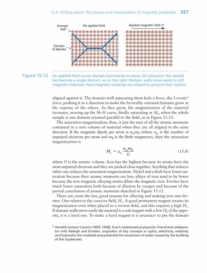
aligned against it. The domain wall separating them feels a force, the Lorentz5
force, pushing it in a direction to make the favorably oriented domains grow atthe expense of the others. As they grow, the magnetization of the materialincreases, moving up the M–H curve, finally saturating at Ms, when the wholesample is one domain oriented parallel to the field, as in Figure 15.13.
The saturation magnetization, then, is just the sum of all the atomic momentscontained in a unit volume of material when they are all aligned in the samedirection. If the magnetic dipole per atom is nmmB (where nm is the number ofunpaired electrons per atom and mB is the Bohr magneton), then the saturationmagnetization is
(15.8)
where Ω is the atomic volume. Iron has the highest because its atoms have themost unpaired electrons and they are packed close together. Anything that reduceseither one reduces the saturation magnetization. Nickel and cobalt have lower sat-uration because their atomic moments are less; alloys of iron tend to be lowerbecause the non-magnetic alloying atoms dilute the magnetic iron. Ferrites havemuch lower saturation both because of dilution by oxygen and because of thepartial cancelation of atomic moments sketched in Figure 15.11.
There are, none the less, good reasons for alloying and making iron into fer-rites. One relates to the coercive field, Hc. A good permanent magnet retains itsmagnetization even when placed in a reverse field, and this requires a high Hc.If domain walls move easily the material is a soft magnet with a low Hc; if the oppo-site, it is a hard one. To make a hard magnet it is necessary to pin the domain
Mn m
s om B µΩ
15.4 Drilling down: the physics and manipulation of magnetic properties 357
5 Hendrik Antoon Lorentz (1853–1928), Dutch mathematical physicist, friend and collabora-tor with Raleigh and Einstein, originator of key concepts in optics, electricity, relativityand hydraulics (he modeled and predicted the movement of water caused by the buildingof the Zuyderzee).
Applied magnetic field HDomain wall
Domainof dipoles
No applied field
Figure 15.13 An applied field causes domain boundaries to move. At saturation the samplehas become a single domain, as on the right. Domain walls move easily in softmagnetic materials. Hard magnetic materials are alloyed to prevent their motion.
Ch15-H8391 1/16/07 6:42 PM Page 357

walls to stop them moving. Impurities, foreign inclusions, precipitates and poros-ity all interact with domain walls, tending to pin them in place (they act as obsta-cles to dislocation motion too, so magnetically hard materials are mechanicallyhard as well). And there are subtler barriers to domain-wall motion: magneticanisotropy arising because certain directions of magnetization in the crystal aremore favorable than others, and even the shape and size of the specimen itself—small, single-domain magnetic particles are particularly resistant to having theirmagnetism reversed.
The performance of a hard magnet is measured by its energy product, roughlyproportional to the area of the magnetization loop. The higher the energy product,the more difficult it is to demagnetize it.
15.5 Materials selection for magnetic design
Selection of materials for their magnetic properties follows the new familiar pat-tern of translating design requirements followed by screening and ranking. In thiscase, however, the first screening step—‘must be magnetic’—immediately isolatesthe special set of materials shown in the property charts of this chapter. The keyselection issue is then whether a soft or hard magnetic response is required.
Soft magnetic devicesElectromagnets, transformers, electron lenses and the like have magnetic coresthat must magnetize easily when the field switches on, be capable of creating ahigh flux density, yet lose their magnetism when the field is switched off. Theydo this by using soft, low Hc, magnetic materials, shown on the left of the chartof Figure 15.8. Soft magnetic materials are used to ‘conduct’ and focus mag-netic flux. Figure 15.14 illustrates this. A current-carrying coil induces a mag-netic field in the core. The field, instead of spreading in the way shown in Figure15.3, is trapped in the extended ferro-magnetic circuit, as shown here. The higherthe susceptibility χ, the greater is the magnetization and flux density induced bya given current loop, up to a limit set by its saturation magnetization Ms. Themagnetic circuit conducts the flux from one coil to another, or from a coil to an
358 Chapter 15 Magnetic materials
Primary Secondary
Soft magnetic
core
Fluxlines
Primary
Fluxintensified
by geometryof core
Soft magnetic
core
Figure 15.14 Soft magnets ‘conduct’ magnetic flux and are concentrated if the cross-sectionof the magnet is reduced.
Ch15-H8391 1/16/07 6:42 PM Page 358

air gap, where it is further enhanced by reducing the section of the core, whereit is used to actuate or to focus an electron beam, as shown on the right ofFigure 15.14. Thus, the first requirement of a good soft magnet is a high χ anda high Ms with a thin hysteresis loop like that sketched in Figure 15.15. The chartof Figure 15.9 shows these two properties. Permendur (Fe–Co–V alloys) andMetglass amorphous alloys are particularly good, but being expensive they areused only in small devices. Silicon–iron (Fe–1–4% Si) is much cheaper and eas-ier to make in large sections; it is the staple material for large transformers.
Most soft magnets are used in AC devices, and then energy loss, proportionalto the area of the hysteresis loop, becomes a consideration. Energy loss is oftwo types: the hysteresis loss already mentioned—it is proportional to switch-ing frequency, f—and eddy current losses caused by the currents induced in thecore itself by the AC field, proportional to f 2. In cores of transformers operat-ing at low frequencies (meaning f up to 100 Hz or so) the hysteresis loss domi-nates, so for these we seek high Ms and a thin loop with a small area. Eddy-currentlosses are present but are suppressed when necessary by laminating: making thecore from a stack of thin sheets interleaved with thin insulating layers that interruptthe eddy currents. At audio frequencies (f 50 kHz) both types of loss becomegreater because they occur on every cycle and now there are more of them, requir-ing an even narrower loop and thinner laminates; here the more expensivePermalloys and Permendurs are used. At higher frequencies still (f in the MHzrange) eddy-current loss, rising with f 2, becomes really serious and the onlyway to stop this is to use magnetic materials that are electrical insulators. Thatmeans ferrites (shown in yellow envelopes on both charts), even though they
15.5 Materials selection for magnetic design 359
Magnetic field H
Magnetization MHigh saturation
magnetization meanshigh flux transfer
Small coercive field Hc means
easy magnetization
Small loop areameans low energy loss
High susceptibility χ(slope of magnetization
curve)
Figure 15.15 A characteristic hysteresis loop for a soft magnet.
Ch15-H8391 1/16/07 6:42 PM Page 359
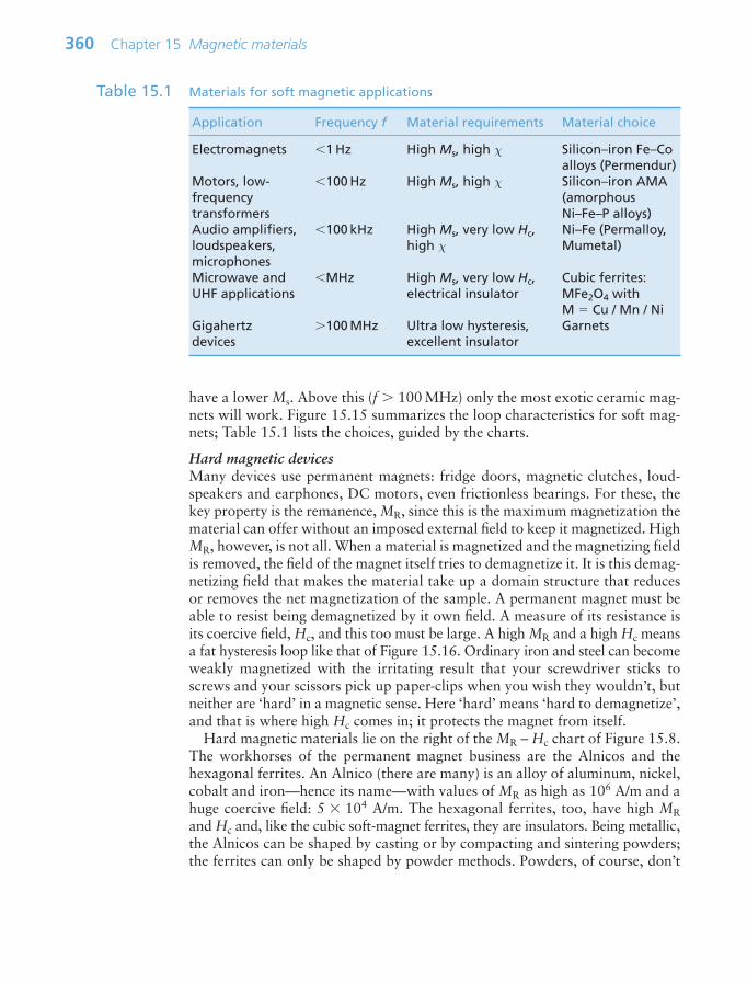
have a lower Ms. Above this (f 100 MHz) only the most exotic ceramic mag-nets will work. Figure 15.15 summarizes the loop characteristics for soft mag-nets; Table 15.1 lists the choices, guided by the charts.
Hard magnetic devicesMany devices use permanent magnets: fridge doors, magnetic clutches, loud-speakers and earphones, DC motors, even frictionless bearings. For these, thekey property is the remanence, MR, since this is the maximum magnetization thematerial can offer without an imposed external field to keep it magnetized. HighMR, however, is not all. When a material is magnetized and the magnetizing fieldis removed, the field of the magnet itself tries to demagnetize it. It is this demag-netizing field that makes the material take up a domain structure that reducesor removes the net magnetization of the sample. A permanent magnet must beable to resist being demagnetized by it own field. A measure of its resistance isits coercive field, Hc, and this too must be large. A high MR and a high Hc meansa fat hysteresis loop like that of Figure 15.16. Ordinary iron and steel can becomeweakly magnetized with the irritating result that your screwdriver sticks toscrews and your scissors pick up paper-clips when you wish they wouldn’t, butneither are ‘hard’ in a magnetic sense. Here ‘hard’ means ‘hard to demagnetize’,and that is where high Hc comes in; it protects the magnet from itself.
Hard magnetic materials lie on the right of the MR – Hc chart of Figure 15.8.The workhorses of the permanent magnet business are the Alnicos and thehexagonal ferrites. An Alnico (there are many) is an alloy of aluminum, nickel,cobalt and iron—hence its name—with values of MR as high as 106 A/m and ahuge coercive field: 5 104 A/m. The hexagonal ferrites, too, have high MRand Hc and, like the cubic soft-magnet ferrites, they are insulators. Being metallic,the Alnicos can be shaped by casting or by compacting and sintering powders;the ferrites can only be shaped by powder methods. Powders, of course, don’t
360 Chapter 15 Magnetic materials
Application Frequency f Material requirements Material choice
Electromagnets 1 Hz High Ms, high χ Silicon–iron Fe–Co alloys (Permendur)
Motors, low- 100 Hz High Ms, high χ Silicon–iron AMA frequency (amorphous transformers Ni–Fe–P alloys)Audio amplifiers, 100 kHz High Ms, very low Hc, Ni–Fe (Permalloy, loudspeakers, high χ Mumetal)microphonesMicrowave and MHz High Ms, very low Hc, Cubic ferrites: UHF applications electrical insulator MFe2O4 with
M Cu / Mn / NiGigahertz 100 MHz Ultra low hysteresis, Garnetsdevices excellent insulator
Table 15.1 Materials for soft magnetic applications
Ch15-H8391 1/16/07 6:42 PM Page 360

have to be sintered—you can bond them together in other ways, and these offeropportunities. Magnetic particles mixed with a resin can be molded to complexshapes. Bonding them with an elastomer gives magnets that are flexible orsquashy—the magnetic seal of a fridge door is an example.
The chart of Figure 15.8 shows three families of hard magnets with coercivefiels that surpass those of Alnicos and hexagonal ferrites. These, the productsof research over the last 30 years, provide the intense permanent-magnet fieldsthat have allowed the miniaturization of earphones, microphones and motors.The oldest of these is the precious metal Pt–Co family but they are so expensivethat they have now all but disappeared. They are outperformed by the cobalt–samarium family based on the inter-metallic compound SmCo5, and they, inturn, are outperformed by the recent development of the neodymium–iron–boronfamily. None of these are cheap, but in the applications they best suit, the quan-tity of material is sufficiently small and the product value sufficiently high thatthis is not an obstacle. Table 15.2 lists the choices, guided by the charts.
Magnetic storage of informationMagnetic information storage requires hard magnets, but ones with an unusualloop shape: one that is rectangular (called ‘square’). The squareness means thata unit of the material can flip in magnetization from MR to MR and backwhen exposed to fields above Hc or Hc. The unit thus stores one binary bitof information. The information is read by moving the magnetized unit past aread head, where it induces an electric pulse. The choice of the word ‘unit’ wasdeliberately vague because it can take several forms: discrete particles embed-ded in a polymer tape or disk, or as a thin magnetic film that has the ability to
15.5 Materials selection for magnetic design 361
Magnetic field H
Magnetization M
High coercive field Hc gives
stable magnetization
Large remanentmagnetization M r gives
powerful magnet
Large loop areagives stable MHmagnetization
Initial magnetization
curve
Figure 15.16 A characteristic hysteresis loop for a hard magnet.
Ch15-H8391 1/16/07 6:42 PM Page 361

carry small stable domains called ‘bubbles’ that are magnetized in one direc-tion, embedded in a background that is magnetized in another.
Figure 15.17 shows one sort of information storage system. A signal creates amagnetic flux in a soft magnetic core—often an amorphous metal alloy (AMA)because of its large susceptibility. The direction of the flux depends on thedirection of the signal current; switching this reverses the direction of the flux.An air gap in the core allows field to escape, penetrating a tape or disk in whichsub-micron particles of a hard magnetic material are embedded. When the sig-nal is in one direction all particles in the band of tape or disk passing under thewrite-head are magnetized in one direction; when the signal is reversed, the direc-tion of magnetization is reversed. The same head is used for reading. When thetape or disk is swept under the air gap, the stray field of the magnetized bandsinduces a flux in the soft iron core and a signal in the coil, which is amplified andprocessed to read it.
362 Chapter 15 Magnetic materials
Application Material requirements Material choice
Large permanent High MR, high Hc and Alnicosmagnets high energy product Hexagonal ferrites
(MH)max; low costSmall high-performance Acoustic, electronic and Cobalt–samariummagnets miniature mechanical Platinum–cobalt
applications Neodymium–boronInformation storage Thin, ‘square’ hysteresis Elongate particles of
loop Fe2O3, Cr2O3 orhexagonal ferrite
Table 15.2 Materials for hard magnetic applications
Magnetic flux (writing) or induced flux (reading)
Metglas soft magnetic core
Recordingtape or disk
Flux penetrates tape (recording);magnetic particles induce flux in head (writing)
Motion of tape or disk
Magnetizedband
Figure 15.17 A magnetic read/write head. The gap in the soft magnetic head allows flux toescape, penetrating the tape and realigning the particles.
Ch15-H8391 1/16/07 6:42 PM Page 362

Why use fine particles? It is because domain walls are not stable in sufficientlysmall particles: each particle is a single domain. If the particle is elongated itprefers to be magnetized parallel to its long axis. Each particle then behaves likea little bar magnet with a north (N) and a south (S) pole at either end. The fieldfrom the write-head is enough to flip the direction, turning an N–S magnetiza-tion into one that is S–N, a binary response that is well suited to informationstorage. Rewritable tapes and disks use particles of Fe2O3 or of CrO2, typically0.1 µm long and with an aspect ratio of 10:1. Particles of hexagonal ferrites (MO)(Fe2O3)6 have a higher coercive field, so a more powerful field is required tochange their magnetization—but having done so, it is hard to erase it. This makesthem the best choice for read-only applications like the identification strip ofcredit and swipe cards.
15.6 Summary and conclusions
The classical picture of an atom is that of a nucleus around which swing elec-trons in discrete orbits, each electron spinning at the same time on its own axis.Both spins create magnetic moments that, if parallel, add up, but if opposed,cancel to a greater or lesser degree. Most materials achieve near-perfect cancel-ation either within the atomic orbits or—if not—by stacking the atomic momentshead to tail or randomizing them so that, when added, they cancel. A very few,most based on just three elements—Fe, Ni and Co—have atoms with residualmoments and an inter-atomic interaction that causes them to line up to give anet magnetic moment or magnetization. Even these materials can find a way toscreen their magnetization by segmenting themselves into domains: a ghetto-likearrangement in which atomic moments segregate into colonies or domains, eachwith a magnetization that is oriented such that it tends to cancel that of its neigh-bors. A strong magnetic field can override the segregation, creating a single unifieddomain in which all the atomic moments are parallel, and if the coercive fieldis large enough, they remain parallel even when the driving field is removed, giv-ing a ‘permanent’ magnetization.
There are two sorts of characters in the world of magnetic materials. There arethose that magnetize readily, requiring only slight urging from an applied fieldto do so. They transmit magnetic flux and require only a small reversal of theapplied field to realign themselves with it. And there are those that, once mag-netized, resist realignment; they give us permanent magnets. The charts of thischapter introduced the two, displaying the properties that most directly deter-mine their choice for a given application.
15.7 Further reading
Braithwaite, N. and Weaver, G. (1990) Electronic Materials, The Open University andButterworth-Heinemann, Oxford, UK. ISBN 0-408-02840-8. (One of the excellentOpen University texts that form part of their Materials program.)
15.7 Further reading 363
Ch15-H8391 1/16/07 6:42 PM Page 363

Campbell, P. (1994) Permanent Magnetic Materials and their Applications, CambridgeUniversity Press, Cambridge, UK.
Douglas, W.D. (1995) Magnetically soft materials, in ASM Metals Handbook, 9th edi-tion, Volume 2, Properties and Selection of Non-ferrous Alloys and Special PurposeMaterials, pp 761–781, ASM, Metals Park, OH, USA.
Fiepke, J.W. (1995) Permanent magnet materials, in ASM Metals Handbook, 9th edi-tion, Volume 2, Properties and Selection of Non-ferrous Alloys and Special PurposeMaterials, pp. 782–803, ASM, Metals Park, OH, USA.
Jakubovics, J.P. (1994) Magnetism and Magnetic Materials, 2nd edition, The Institute ofMaterials, London, UK. ISBN 0-901716-54-5. (A simple introduction to magneticmaterials, short and readable.)
364 Chapter 15 Magnetic materials
15.8 Exercises
Exercise E15.1 Sketch an Ms–H curve for a ferro-magnetic material. Identify the importantmagnetic properties.
Exercise E15.2 Why are some elements ferro-magnetic when others are not?
Exercise E15.3 What is a ferrite? What are its characteristics?
Exercise E15.4 What is a Bohr magneton? A magnetic element has two unpaired electrons andan exchange interaction that causes them to align such that their magneticfields are parallel. Its atomic volume, Ω, is 3.7 1029 m3. What would youexpect its saturation magnetization, Ms, to be?
Exercise E15.5 A coil of 50 turns and length 10 mm carries a current of 0.01 amps. The coreof the coil is made of a material with a susceptibility χ 104. What is themagnetization M and the induction B?
Exercise E15.6 An inductor core is required for a low-frequency harmonic filter. Therequirement is for low loss and high saturation magnetization. Using thecharts of Figures 15.8 and 15.9 as data sources, which class of magnetic mate-rial would you choose?
Exercise E15.7 A magnetic material is required for the core of a transformer that forms partof a radar speed camera. It operates at a microwave frequency of 500 kHz.Which class of material would you choose?
Exercise E15.8 A material is required for a flexible magnetic seal. It must be in the form ofan elastomeric sheet and must be electrically insulating. How would you pro-pose to make such a material?
Exercise E15.9 What are the characteristics required of materials for magnetic informationstorage?
Ch15-H8391 1/16/07 6:42 PM Page 364
15.9 Exploring design with CES 365
15.9 Exploring design with CES
Open CES at Level 3—it opens in the ‘Browse’ mode. At the head of theBrowse list are two pull-down menus reading ‘Table’ and ‘Subset’. Open the‘Subset’ menu and choose ‘Magnetic’. Records for 233 magnetic materials aredisplayed, listing their magnetic properties and, where available, mechanical,thermal, electrical and other properties too.
To select, click on ‘Select’ in the main toolbar and choose MaterialsUniverse Magnetic materials in the dialog box. Now we can begin.
Exercise E15.10 Use the CES ‘Search’ facility to find materials for:
(a) Transformer cores.(b) Electric motors.
Exercise E15.11 Find by browsing the records for:
(a) Cast Alnico 3. What is the value of its coercive force Hc?(b) The amorphous alloy Metglas 2605-Co. What is the value of its coercive
force Hc?
What do these values tell you about the potential applications of these twomaterials?
Exercise E15.12 Find by browsing the records for:
(a) Ferrite G (Ni–Zn ferrite). What are the values of its coercive forceHc and resistivity ρe?
(b) 2.5Si–Fe soft magnetic alloy. What are the values of its coercive forceHc and resistivity ρe?
If you were asked to choose one of these for a transformer core, what wouldbe your first question?
Exercise E15.13 Make a bar chart of saturation induction Bs (the saturation magnetizationMs Bs/µo, so the two are proportional). Report the three materials withthe highest values.
Exercise E15.14 Make a bar chart of coercive force, Hc. Report the four materials with thelowest value. What applications use them?
Exercise E15.15 A soft magnetic material is required for the laminated rotor of an AC induc-tion electric motor. The material is to be rolled and further shaped by stamp-ing, requiring an elongation of at least 40%. To keep hysteresis losses to aminimum it should have the lowest possible coercive force. Find the twomaterials that best meet these requirements, summarized below. Report themand their trade names.
Ch15-H8391 1/16/07 6:42 PM Page 365

366 Chapter 15 Magnetic materials
Exercise E15.16 A magnetic material is required for the read/write head of a hard disk drive.It must have high hardness to resist wear and the lowest possible coerciveforce to give accurate read/write response.
(a) Use CES to identify possible candidates that meet these requirements,summarized in the table.
(b) Now add the further constraint that, for lower loss and high-frequencydamping, the magnetic material must have an electrical resistivity above108 µΩ. cm.
Function • Motor laminations
Constraints • Soft magnetic material• Ductile (elongation 40%)
Objective • Minimize coercive force
Free variable • Choice of material
Function • Magnetic read-head
Constraints • Soft magnetic material• High hardness for wear resistance (Vickers
hardness 500 HV)
Objective • Minimize coercive force
Free variable • Choice of material
15.10 Exploring the science with CES Elements
Exercise E15.17 Make a chart with atomic number on the x-axis and magneton moment peratom (Bohr magneton) on the y-axis (use linear scales) to identify the ferro-magnetic elements. How many are there? Which have the highest magnetonmoment per atom?
Exercise E15.18 According to equation (15.8) of the text, the saturation magnetization is
where nm is the magnetic dipole per atom in units of Bohr magnetons, Ω isthe atomic volume, mB is the value of a Bohr magneton (9.3 1024A/m2)and µo the permeability of a vacuum (µo 4π 107H/m). Make a chartwith this combination of properties on the x-axis and the saturation magne-tization Ms on the y-axis for the elements of the Periodic Table. How accu-rately is this equation obeyed?
Mn m
s om B µΩ
Ch15-H8391 1/16/07 6:42 PM Page 366

Chapter 16Materials for optical devices
Chapter contents
16.1 Introduction and synopsis 36816.2 The interaction of materials and
radiation 36816.3 Charts for optical properties 37316.4 Drilling down: the physics and
manipulationof optical properties 375
16.5 Optical design 38116.6 Summary and conclusions 38216.7 Further reading 38316.8 Exercises 38316.9 Exploring design with CES 38416.10 Exploring the science with CES
Elements 385
Instruments using the ability of materials to reflectand refract. (Image of microscope courtesy of A–Z
Microscope Corporation, California USA.)
Ch16-H8391.qxd 1/16/07 6:42 PM Page 367

368 Chapter 16 Materials for optical devices
16.1 Introduction and synopsis
It was at one time thought that the fact that light could travel through space—from the sun to earth, for instance—must mean that space was not really emptybut filled with ‘luminiferous ether’. It was not until the experiments ofMichelson1 and Morley in 1881 that it was realized that light did not need a‘material’ for its propagation but could propagate through totally empty spaceat what is now seen as the ultimate velocity: 3 108m/s.
When radiation strikes materials, things can happen. Materials interact withradiation by reflecting it, absorbing it, transmitting it and refracting it. This chap-ter is about these interactions, the materials that do them best and the ways we usethem. The chapter opening page shows two: a reflecting telescope and a refract-ing microscope, each of which depend on the optical properties of materials.
16.2 The interaction of materials and radiation
Electromagnetic (e-m) radiation permeates the entire universe. Observe the skywith your eye and you see the visible spectrum, the range of wavelengths wecall ‘light’ (0.40–0.77 µm). Observe it with a detector of X-rays or γ-rays and yousee radiation with far shorter wavelengths (as short as 104nm, one-thousandththe size of an atom). Observe it instead with a radio-telescope and you pick upradiation with wavelengths measured in millimeters, meters or even kilometers,known as radio and microwaves. The range of wavelengths of radiation is vast,spanning 18 orders of magnitude (Figure 16.1). The visible part of this spec-trum is only a tiny part of it—but even that has entrancing variety, giving uscolors ranging from deep purple through blue, green and yellow to deep red.
The intensity I of an e-m wave, proportional to the square of its amplitude,is a measure of the energy it carries. When radiation with intensity Io strikes amaterial, a part IR of it is reflected, a part IA absorbed and a part IT may betransmitted. Conservation of energy requires that
(16.1)
The first term is called the reflectivity of the material, the second the absorptiv-ity and the last the transmittability (all dimensionless). Each depends on thewavelength of the radiation, on the nature of the material and on the state of
I
I
I
I
I
IR
o
A
o
T
o
1
1Albert A. Michelson (1852–1931), Prussian-American experimental physicist, who, withE.W. Morley, first demonstrated that the speed of light is independent of the earth’smotion, a finding central to the establishment of the theory of relativity.
Ch16-H8391.qxd 1/16/07 6:42 PM Page 368

16.2 The interaction of materials and radiation 369
its surfaces. They can be thought of as properties of the material in a given stateof surface polish, smoothness or roughness.
In optics we are concerned with wavelengths in the visible spectrum. Materialsthat reflect or absorb all visible light, transmitting none, are called opaque, eventhough they may transmit in the near visible (infrared or ultraviolet). Thosethat transmit a little diffuse light are called translucent. Those that transmitlight sufficiently well that you can see through them are called transparent; asubset of these that transmit almost perfectly, making them suitable for lenses,light-guides and optical fibers, are given the additional title of optical quality.Metals are opaque. To be transparent a material must be a dielectric.
Specular and diffuse reflectionMetals reflect almost all the light that strikes them; none is transmitted and lit-tle is absorbed. When light strikes a reflecting surface at an incident angle θ1,part of it is reflected, leaving the surface with an angle of reflection θ2 such that
(16.2)
Specular surfaces are microscopically smooth and flat. A beam striking such asurface suffers specular reflection, meaning that it is reflected as a beam, as on
θ θ1 2
Freq
uenc
y (H
z)
1020
1017
1011
1014
108
105
Wav
elen
gth
(m)
103
1
10−3
10−6
10−9
10−12
Radio waves
Microwaves
Infrared
Visible light
Ultraviolet
X-rays
Gamma rays
0.77 µm
0.4 µm
Red
Orange
Yellow
Green
Blue
Violet
Figure 16.1 The spectrum of electromagnetic (e-m) waves. The visible spectrum lies betweenthe wavelengths 0.4 and 0.77 µm.
Ch16-H8391.qxd 1/16/07 6:42 PM Page 369

the left of Figure 16.2. Diffuse surfaces are irregular; the law of reflection(equation (16.2)) still holds locally but the incident beam is reflected in manydifferent directions because of the irregularities, as on the right of the figure.
AbsorptionIf radiation can penetrate a material, some is absorbed. The greater the thick-ness x through which the radiation passes, the greater the absorption. Theintensity I, starting with the initial value I0, decreases such that
(16.3)
where β is the absorption coefficient, with dimensions of m1 (or, more conve-niently, mm1). The absorption coefficient depends on wavelength, with theresult that white light passing through a material may emerge with a color cor-responding to the wavelength that is least absorbed—that is why a thick slab ofice looks blue.
TransmissionBy the time a beam of light has passed completely through a slab of material ithas lost some intensity through reflection at the surface at which it entered,some in reflection at the surface at which it leaves, and some by absorption inbetween. Its intensity is
(16.4)
The term (1 IR/Io) occurs to the second power because intensity is lostthrough reflection at both surfaces.
I II
Ix o
R
o
exp12⎛
⎝⎜⎜⎜⎜
⎞
⎠⎟⎟⎟⎟⎟
β
I I x o exp β
370 Chapter 16 Materials for optical devices
Incidentbeam
Reflectedbeam
θ1 θ2
Incidentbeam
Scatteredbeams
Figure 16.2 Optically flat, reflective surfaces give specular reflection, such that θ1 θ2. Theangles of incidence and reflection are always equal, but the rough surface givesdiffuse reflection even though the angles of incidence and reflection are still,locally, equal.
Ch16-H8391.qxd 1/16/07 6:42 PM Page 370

RefractionThe velocity of light in a vacuum, co3 108m/s, is as fast as it ever goes.When it (or any other electromagnetic radiation) enters a material, it slowsdown. The index of refraction, n, is the ratio of its velocity in a vacuum, co, tothat in the material, c:
(16.5)
This retardation makes a beam of light bend or refract when it enters a mate-rial of different refractive index. When a beam passes from a material 1 ofrefractive index n1 into a material 2 of index n2 with an angle of incidence θ1,it deflects to an angle θ2, such that
(16.6)
as in Figure 16.3(a); the equation is known as Snell’s law2. The refractive indexdepends on wavelength, so each of the colors that make up white light is dif-fracted through a slightly different angle, producing a spectrum when lightpasses through a prism. When material 1 is vacuum or air, for which n1 1,the equation reduces to
Equation (16.6) says that light passes from a material with index n1 n intoair with n2 1, it is bent away from the normal to the surface, like that inFigure 16.3(b). If the incident angle, here θ1, is slowly increased, the emergingbeam tips down until it becomes parallel with the surface when θ2 90° andsin θ2 1. This occurs at an incident angle, from equation (16.6), of
(16.7)
For values of θ1 greater than this, the equation predicts values of sin θ2 that aregreater than 1, and that can’t be. Something strange has to happen, and it does:the ray is totally reflected back into the material, as in Figure 16.3(c). This total
sin θ11
n
sinsin
θθ
1
22 n
sinsin
θθ
1
2
2
1
n
n
nc
c o
16.2 The interaction of materials and radiation 371
2Willebrord Snell (1591–1626), Dutch astronomer, also known as Snell van Royen, orSnellius, who first derived the relationship between the different angles of light as it passesfrom one transparent medium to another. The lunar crater Snellius is named after him.
Ch16-H8391.qxd 1/16/07 6:42 PM Page 371

internal reflection has many uses, one being to bend the path of light in pris-matic binoculars and reflex cameras. Another is to trap light within an opticalfiber, an application that has changed the way we communicate.
Reflection is related to refraction. When light traveling in a material ofrefractive index n1 is incident normal to the surface of a second material with arefractive index n2, the reflectivity is
(16.8a)
If the incident beam is in air, with refractive index 1, this becomes
(16.8b)
Thus, materials with high refractive index have high reflectivity.Before leaving Snell and his law, ponder for a moment on the odd fact that
the beam is bent at all. Light entering a dielectric, as we have said, slows down.
RI
Inn
R
o
11
2⎛
⎝⎜⎜⎜
⎞
⎠⎟⎟⎟⎟
RI
I
n n
n n
R
o
2 1
2 1
2⎛
⎝⎜⎜⎜⎜
⎞
⎠⎟⎟⎟⎟⎟
372 Chapter 16 Materials for optical devices
θ1
θ2
Incidentbeam
Refractedbeam
Material, refractiveindex n
Vacuum (or air)
θ1Incidentbeam
Refractedbeam
Material,refractive index n
Vacuum (or air)
θ2
θ1
Incidentbeam
Reflectedbeam
Material,refractive index n
Vacuum (or air)
θ1
(a)
(b) (c)
sin θ1sin θ2
n =
Figure 16.3 Refraction and total internal reflection.
Ch16-H8391.qxd 1/16/07 6:42 PM Page 372
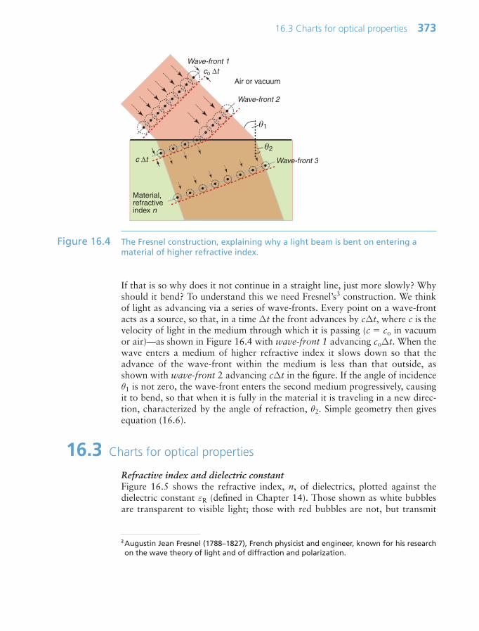
If that is so why does it not continue in a straight line, just more slowly? Whyshould it bend? To understand this we need Fresnel’s3 construction. We thinkof light as advancing via a series of wave-fronts. Every point on a wave-frontacts as a source, so that, in a time ∆t the front advances by c∆t, where c is thevelocity of light in the medium through which it is passing (c co in vacuumor air)—as shown in Figure 16.4 with wave-front 1 advancing co∆t. When thewave enters a medium of higher refractive index it slows down so that theadvance of the wave-front within the medium is less than that outside, asshown with wave-front 2 advancing c∆t in the figure. If the angle of incidenceθ1 is not zero, the wave-front enters the second medium progressively, causingit to bend, so that when it is fully in the material it is traveling in a new direc-tion, characterized by the angle of refraction, θ2. Simple geometry then givesequation (16.6).
16.3 Charts for optical properties
Refractive index and dielectric constantFigure 16.5 shows the refractive index, n, of dielectrics, plotted against thedielectric constant εR (defined in Chapter 14). Those shown as white bubblesare transparent to visible light; those with red bubbles are not, but transmit
16.3 Charts for optical properties 373
Air or vacuum
Material, refractiveindex n
Wave-front 2
Wave-front 3
Wave-front 1
θ1
θ2
co ∆t
c ∆t
Figure 16.4 The Fresnel construction, explaining why a light beam is bent on entering amaterial of higher refractive index.
3Augustin Jean Fresnel (1788–1827), French physicist and engineer, known for his researchon the wave theory of light and of diffraction and polarization.
Ch16-H8391.qxd 1/16/07 6:42 PM Page 373
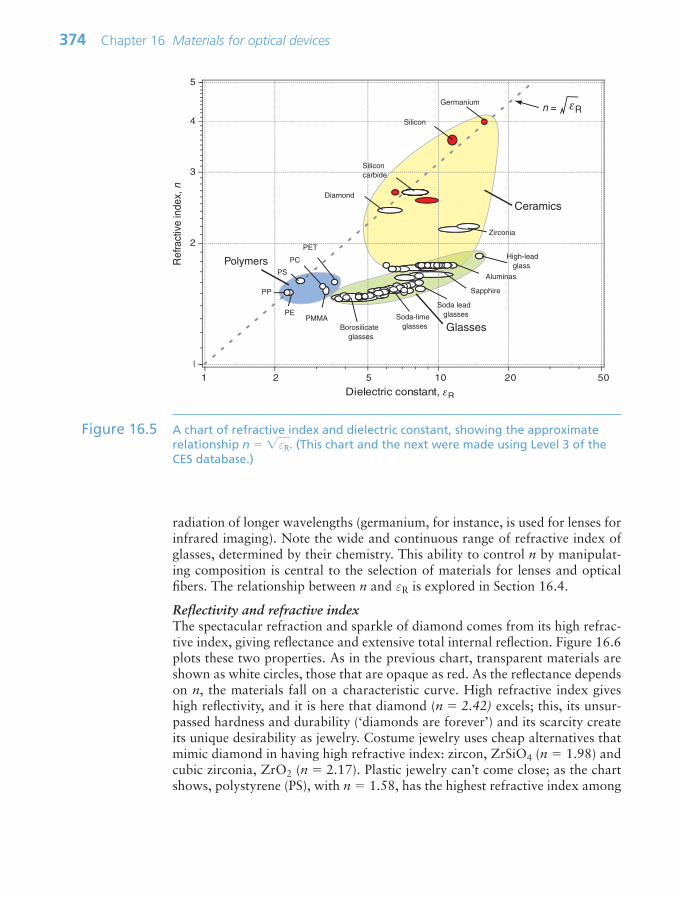
radiation of longer wavelengths (germanium, for instance, is used for lenses forinfrared imaging). Note the wide and continuous range of refractive index ofglasses, determined by their chemistry. This ability to control n by manipulat-ing composition is central to the selection of materials for lenses and opticalfibers. The relationship between n and εR is explored in Section 16.4.
Reflectivity and refractive indexThe spectacular refraction and sparkle of diamond comes from its high refrac-tive index, giving reflectance and extensive total internal reflection. Figure 16.6plots these two properties. As in the previous chart, transparent materials areshown as white circles, those that are opaque as red. As the reflectance dependson n, the materials fall on a characteristic curve. High refractive index giveshigh reflectivity, and it is here that diamond (n 2.42) excels; this, its unsur-passed hardness and durability (‘diamonds are forever’) and its scarcity createits unique desirability as jewelry. Costume jewelry uses cheap alternatives thatmimic diamond in having high refractive index: zircon, ZrSiO4 (n 1.98) andcubic zirconia, ZrO2 (n 2.17). Plastic jewelry can’t come close; as the chartshows, polystyrene (PS), with n 1.58, has the highest refractive index among
374 Chapter 16 Materials for optical devices
Dielectric constant, εR
Ref
ract
ive
inde
x, n
1
2
3
4
5
1 2 5 10 20 50
n = εRGermanium
Silicon
Diamond
Silicon carbide
PP
PE
PS
PET
PMMA
PC
Zirconia
High-lead glass
Aluminas
Soda lead glassesSoda-lime
glassesBorosilicate glasses
Sapphire
Ceramics
Glasses
Polymers
Figure 16.5 A chart of refractive index and dielectric constant, showing the approximaterelationship n εR. (This chart and the next were made using Level 3 of theCES database.)
Ch16-H8391.qxd 1/16/07 6:42 PM Page 374

polymers (one reason it is used for the so-called ‘jewel’ cases in which CDs arepackaged) but it is much lower than those of real jewels.
16.4 Drilling down: the physics and manipulation of opticalproperties
Light, like all radiation, is an electromagnetic (e-m) wave. The coupled fields aresketched in Figure 16.7. The electric part fluctuates with a frequency ν that deter-mines where it lies in the spectrum of Figure 16.1. A fluctuating electric fieldinduces a fluctuating magnetic field that is exactly π/2 out of phase with theelectric one, because the induction is at its maximum when the electric field ischanging most rapidly. A plane-polarized beam looks like this one: the electricand magnetic fields lie in fixed planes. Natural light is not polarized; then thewave also rotates so that the plane containing each wave continuously changes.
Many aspects of radiation are most easily understood by thinking of it as awave. Others need a different picture—that of radiation as discrete packets of
16.4 Drilling down: the physics and manipulation of optical properties 375
Refractive index, n
21 3 4 5
Ref
lect
ance
, ((
n −
1)/(n
+ 1
))2
0.2
0.02
0.05
0.1
0.5Germanium
Silicon
Siliconcarbide
Titaniumdioxide
Diamond
Zirconia
High-lead glasses
Sapphire
PMMA
PP
PEPS
Borosilicate glasses
Soda leadglasses
Sodaglasses
PET
PC
Ceramics
Polymers
Glasses
Figure 16.6 A chart of refractive index and reflectance. The materials with open circles aretransparent to visible light; those with red circles are transparent to infraredand below, but not to visible radiation. Diamond is special because of its highrefractive index, reflectance and transparency in the visible spectrum.
Ch16-H8391.qxd 1/16/07 6:42 PM Page 375

energy, photons. The idea of a wave that is also discrete energy units is not intuitive—it is another of the results of quantum theory that do not correspondto ordinary experience. The energy Eph of a photon of radiation of frequency νor wavelength λ is
(16.9)
where h is Planck’s4 constant (6.626 1034J.s) and c is the speed of the radi-ation. Thus, radiation of a given frequency has photons of fixed energy, regard-less of its intensity—an intense beam simply has more of them. This is the keyto understanding reflection, absorption and transmission.
Why aren’t metals transparent?Recall from Chapter 14 that the electrons in materials circle their parent atomin orbits with discrete energy levels, and only two can occupy the same level.Metals have an enormous number of very closely spaced levels in their conduc-tion band; the electrons in the metal only fill part of this number. Filling the lev-els in a metal is like pouring water into a container until it is part full—itssurface is the Fermi5 level; levels above it are empty. If you ‘excite’ the water—say, by shaking the container—some of it can slosh to a higher level. If you stopsloshing, it will return to its Fermi level.
Radiation excites electrons; and in metals there are plenty of empty levels inthe conduction band into which they can be excited. But here quantum effectscut in. A photon with energy hν can excite an electron only if there is an energylevel that is exactly hν above the Fermi level—and in metals there is. So all thephotons of a light beam are captured by electrons of a metal, regardless of theirwavelength. Figure 16.8 shows, on the left, what happens to just one.
E hhc
ph νλ
376 Chapter 16 Materials for optical devices
Electric field E
Magnetic field H
Wavelength λ
Figure 16.7 An electromagnetic wave. The electric component (gray) is π/2 out of phasewith the magnetic component (red).
4Max Karl Ernst Ludwig Planck (1858–1947), a central figure in the development of quan-tum theory; it was he who formulated equation (16.9).
5Enrico Fermi (1901–1954), devisor of the statistical laws known as Fermi statistics governingthe behavior of electrons in solids. He was one of the leaders of the team of physicists onthe Manhattan Project for the development of the atomic bomb.
Ch16-H8391.qxd 1/16/07 6:42 PM Page 376
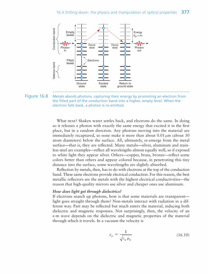
What next? Shaken water settles back, and electrons do the same. In doingso it releases a photon with exactly the same energy that excited it in the firstplace, but in a random direction. Any photons moving into the material areimmediately recaptured, so none make it more than about 0.01 µm (about 30atom diameters) below the surface. All, ultimately, re-emerge from the metalsurface—that is, they are reflected. Many metals—silver, aluminum and stain-less steel are examples—reflect all wavelengths almost equally well, so if exposedto white light they appear silver. Others—copper, brass, bronze—reflect somecolors better than others and appear colored because, in penetrating this tinydistance into the surface, some wavelengths are slightly absorbed.
Reflection by metals, then, has to do with electrons at the top of the conductionband. These same electrons provide electrical conduction. For this reason, the bestmetallic reflectors are the metals with the highest electrical conductivities—thereason that high-quality mirrors use silver and cheaper ones use aluminum.
How does light get through dielectrics?If electrons snatch up photons, how is that some materials are transparent—light goes straight through them? Non-metals interact with radiation in a dif-ferent way. Part may be reflected but much enters the material, inducing bothdielectric and magnetic responses. Not surprisingly, then, the velocity of an e-m wave depends on the dielectric and magnetic properties of the materialthrough which it travels. In a vacuum the velocity is
(16.10)coo o
1
ε µ
16.4 Drilling down: the physics and manipulation of optical properties 377
Ground state
Fermilevel
Fermilevel
EnergyEp = hν
ElectronsFilledlevels
Emptylevels
Photonin
Excitedstate
Return toground state
Photonout
Val
ence
ban
dC
ondu
ctio
n ba
nd
Figure 16.8 Metals absorb photons, capturing their energy by promoting an electron fromthe filled part of the conduction band into a higher, empty level. When theelectron falls back, a photon is re-emitted.
Ch16-H8391.qxd 1/16/07 6:42 PM Page 377
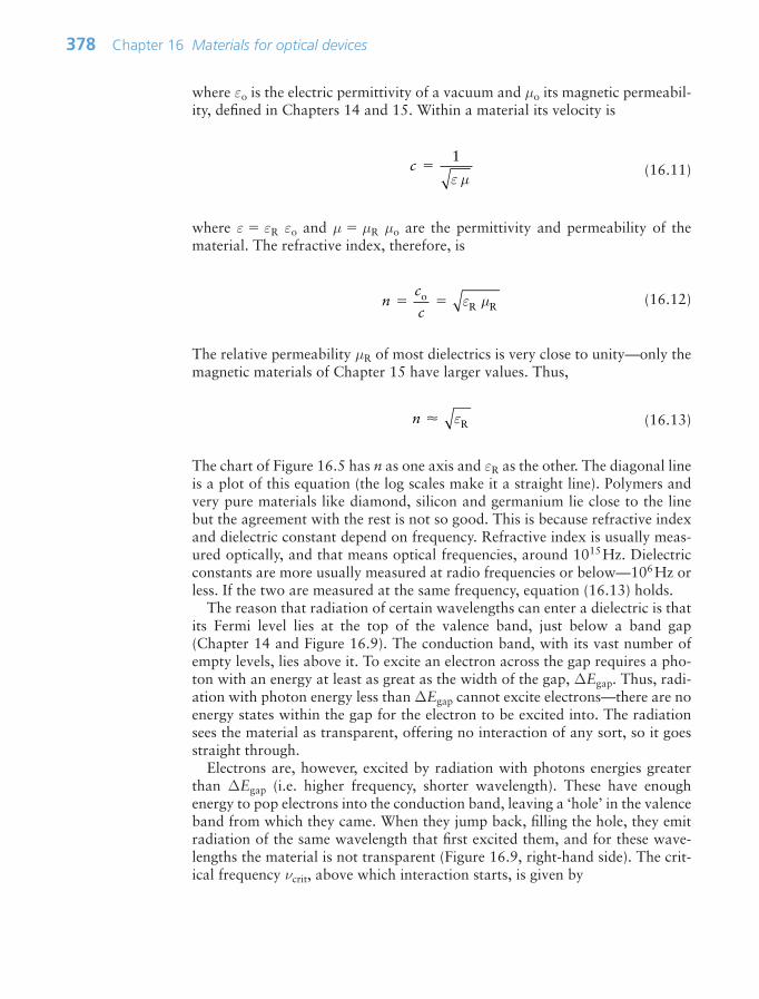
where εo is the electric permittivity of a vacuum and µo its magnetic permeabil-ity, defined in Chapters 14 and 15. Within a material its velocity is
(16.11)
where ε εR εo and µ µR µo are the permittivity and permeability of thematerial. The refractive index, therefore, is
(16.12)
The relative permeability µR of most dielectrics is very close to unity—only themagnetic materials of Chapter 15 have larger values. Thus,
(16.13)
The chart of Figure 16.5 has n as one axis and εR as the other. The diagonal lineis a plot of this equation (the log scales make it a straight line). Polymers andvery pure materials like diamond, silicon and germanium lie close to the linebut the agreement with the rest is not so good. This is because refractive indexand dielectric constant depend on frequency. Refractive index is usually meas-ured optically, and that means optical frequencies, around 1015Hz. Dielectricconstants are more usually measured at radio frequencies or below—106Hz orless. If the two are measured at the same frequency, equation (16.13) holds.
The reason that radiation of certain wavelengths can enter a dielectric is thatits Fermi level lies at the top of the valence band, just below a band gap(Chapter 14 and Figure 16.9). The conduction band, with its vast number ofempty levels, lies above it. To excite an electron across the gap requires a pho-ton with an energy at least as great as the width of the gap, ∆Egap. Thus, radi-ation with photon energy less than ∆Egap cannot excite electrons—there are noenergy states within the gap for the electron to be excited into. The radiationsees the material as transparent, offering no interaction of any sort, so it goesstraight through.
Electrons are, however, excited by radiation with photons energies greaterthan ∆Egap (i.e. higher frequency, shorter wavelength). These have enoughenergy to pop electrons into the conduction band, leaving a ‘hole’ in the valenceband from which they came. When they jump back, filling the hole, they emitradiation of the same wavelength that first excited them, and for these wave-lengths the material is not transparent (Figure 16.9, right-hand side). The crit-ical frequency νcrit, above which interaction starts, is given by
n εR
nc
c o
R Rε µ
c 1
ε µ
378 Chapter 16 Materials for optical devices
Ch16-H8391.qxd 1/16/07 6:42 PM Page 378
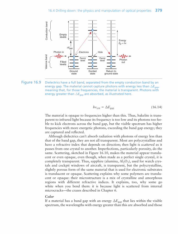
hνcrit ∆Egap (16.14)
The material is opaque to frequencies higher than this. Thus, bakelite is trans-parent to infrared light because its frequency is too low and its photons too fee-ble to kick electrons across the band gap, but the visible spectrum has higherfrequencies with more energetic photons, exceeding the band gap energy; theyare captured and reflected.
Although dielectrics can’t absorb radiation with photons of energy less thanthat of the band gap, they are not all transparent. Most are polycrystalline andhave a refractive index that depends on direction; then light is scattered as itpasses from one crystal to another. Imperfections, particularly porosity, do thesame. Scattering, sketched in Figure 16.10, makes the material appear translu-cent or even opaque, even though, when made as a perfect single crystal, it iscompletely transparent. Thus, sapphire (alumina, Al2O3), used for watch crys-tals and cockpit windows of aircraft, is transparent, but the polycrystalline,slightly porous form of the same material that is used for electronic substratesis translucent or opaque. Scattering explains why some polymers are translu-cent or opaque: their microstructure is a mix of crystalline and amorphousregions with different refractive indices. It explains, too, why some go white when you bend them: it is because light is scattered from internal microcracks—the crazes described in Chapter 6.
ColorIf a material has a band gap with an energy ∆Egap that lies within the visiblespectrum, the wavelengths with energy greater than this are absorbed and those
16.4 Drilling down: the physics and manipulation of optical properties 379
Ground state
Fermilevel
Fermilevel
EnergyEp = hν
HoleElectrons
Filledlevels
Emptylevels
Photon in
Excitedstate
Return toground state
Photonout
∆EgapV
alen
ce b
and
Con
duct
ion
band
Figure 16.9 Dielectrics have a full band, separated from the empty conduction band by anenergy gap. The material cannot capture photons with energy less than ∆Egap,meaning that, for those frequencies, the material is transparent. Photons withenergy greater than ∆Egap are absorbed, as illustrated here.
Ch16-H8391.qxd 1/16/07 6:42 PM Page 379

with energy that is less are not. The absorbed radiation is re-emitted when theexcited electron drops back into a lower energy state, but this may not be the one it started from, so the photon it emits has a different wavelength thanthe one that was originally absorbed. The light emitted from the material is amix of the transmitted and the re-emitted wavelengths, and it is this that givesit a characteristic color.
More specific control of color is possible by doping—the deliberate introduc-tion of impurities that create a new energy level in the band gap, as in Figure16.11. Radiation is absorbed as before but it is now re-emitted in two discretesteps as the electrons drop first into the dopant level, emitting a photon of fre-quency ν1 ∆E1/h and from there back into the valence band, emitting a sec-ond photon of energy ν2 ∆E2/h. Particularly pure colors are created whenglasses are doped with metal ions: copper gives blue; cobalt, violet; chromium,green; manganese, yellow.
Fluorescence, phosphorescence and electro luminescenceElectrons can be excited into higher energy levels by incident photons, providedthey have sufficient energy. Energetic electrons, like those of the electron beamof a cathode ray tube, do the same. In most materials the time delay before theydrop back into lower levels, re-emitting the energy they captured, is extremelyshort, but in some there is a delay. If, on dropping back, the photon they emitis in the visible spectrum, the effect is that of luminescence—the material con-tinues to glow even when the incident beam is removed. When the time delay isfractions of seconds, it is called fluorescence, used in fluorescent lighting, whereit is excited by ultraviolet from a gas discharge, and in TV tubes where it isexcited by the scanning electron beam. When the time delay is longer it is calledphosphorescence; it is no longer useful for creating moving images but is usedinstead for static displays like that of watch faces, where it is excited by elec-trons (β-particles) released by a mildly radioactive ingredient in the paint.
380 Chapter 16 Materials for optical devices
(a) (b)
Figure 16.10 (a) A pure glass with no internal structure and a wide band gap is completelytransparent. (b) Light entering a polycrystalline ceramic or a partly crystallinepolymer suffers multiple refraction and is also scattered by porosity, making ittranslucent.
Ch16-H8391.qxd 1/16/07 6:42 PM Page 380
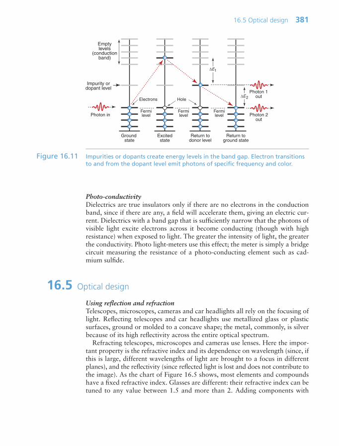
Photo-conductivityDielectrics are true insulators only if there are no electrons in the conductionband, since if there are any, a field will accelerate them, giving an electric cur-rent. Dielectrics with a band gap that is sufficiently narrow that the photons ofvisible light excite electrons across it become conducting (though with highresistance) when exposed to light. The greater the intensity of light, the greaterthe conductivity. Photo light-meters use this effect; the meter is simply a bridgecircuit measuring the resistance of a photo-conducting element such as cad-mium sulfide.
16.5 Optical design
Using reflection and refractionTelescopes, microscopes, cameras and car headlights all rely on the focusing oflight. Reflecting telescopes and car headlights use metallized glass or plasticsurfaces, ground or molded to a concave shape; the metal, commonly, is silverbecause of its high reflectivity across the entire optical spectrum.
Refracting telescopes, microscopes and cameras use lenses. Here the impor-tant property is the refractive index and its dependence on wavelength (since, ifthis is large, different wavelengths of light are brought to a focus in differentplanes), and the reflectivity (since reflected light is lost and does not contribute tothe image). As the chart of Figure 16.5 shows, most elements and compoundshave a fixed refractive index. Glasses are different: their refractive index can betuned to any value between 1.5 and more than 2. Adding components with
16.5 Optical design 381
Ground state
Fermilevel
HoleElectrons
Emptylevels
(conductionband)
Impurity ordopant level
Photon in
Excitedstate
Return todonor level
Photon 2out
Fermilevel
Fermilevel
∆E2
∆E1
Photon 1out
Return toground state
Figure 16.11 Impurities or dopants create energy levels in the band gap. Electron transitionsto and from the dopant level emit photons of specific frequency and color.
Ch16-H8391.qxd 1/16/07 6:42 PM Page 381

light elements like sodium (as in soda-lime glass) gives a low refractive index;adding heavy elements like lead (as in lead glass or ‘crystal’) gives a high one.
Using total internal reflectionOptical fibers have revolutionized the digital transmission of information:almost all landlines now use these rather than copper wires as the ‘conductor’.A single fiber consists of a core of pure glass contained in a cladding of anotherglass with a lower refractive index, as in Figure 16.12. A digitized signal is con-verted into optical pulses by a light-emitting diode and is fed into the fiber,where it is contained within the core, even when the fiber is bent, because anyray striking the core–cladding interface at a low angle suffers total internalreflection. The purity of the core—a silica glass—is so high that absorption isvery small; occasional repeater stations are needed to receive, amplify andretransmit the signal to cover long distances.
16.6 Summary and conclusions
Materials interact with electromagnetic radiation in several ways: reflecting it,refracting it and absorbing it. This is because radiation behaves both as a waveof frequency ν and as a stream of discrete photons with energy Eph hν.Electrons in materials capture photons, grabbing their energy, provided thereare energy levels exactly Eph above their ground state for them to occupy. Aftera time delay that is usually very short, the electrons drop back down to theirground state, re-emitting their energy as new photons. In metals there arealways usable energy levels so every photon hitting a metal is captured andthrown back out, giving reflection. In a dielectric, the atoms ignore low-frequency, low-energy photons and capture only those with energy above a crit-ical level set by the band gap. Those that are not caught pass straight through;for these frequencies, the material is transparent. Doping introduces extra slotswithin the band gap for electrons to fall into as they release their energy, and indoing so they emit photons of specific frequency and color.
When radiation enters a dielectric, it slows down. A consequence of this isthat a beam entering at an angle is bent—the phenomenon of refraction. It is
382 Chapter 16 Materials for optical devices
Cladding of lowerrefractive index
Core
Figure 16.12 An optical fiber. The graded refractive index traps light by total internalreflection, making it follow the fiber even when it is curved.
Ch16-H8391.qxd 1/16/07 6:42 PM Page 382

this that allows light to be focused by lenses, reflected by prisms and trapped infine, transparent fibers to transmit information.
Of all the transparent materials at our disposal, glasses offer the greatest rangeof refractive index and color. Glasses are based on amorphous silica, SiO2. Silicais an extremely good solvent, allowing a wide range of other oxides to be dis-solved in it over a wide range of concentrations. It is this that allows the opti-cal properties of glasses to be adjusted and fine-tuned to match design needs.
16.7 Further reading
Callister, W.D., Jr (2003) Materials science and engineering, An Introduction, 6th edi-tion, John Wiley, New York, USA. ISBN 0-471-13576-3. (A well-established andcomprehensive introduction to the science of materials.)
Jiles, D. (2001) Introduction to the Electronic Properties of Materials, NelsonThompson, Cheltenham, UK. ISBN 0-7487-6042-3. (A refreshingly direct approachto the thermal, electrical, magnetic and optical properties of materials and their elec-tronic origins.)
16.8 Exercises 383
16.8 Exercises
Exercise E16.1 Define refractive index. Give examples of devices that make use of refraction.
Exercise E16.2 Define reflectance. Give examples of devices that make use of reflection.
Exercise E16.3 The absorption coefficient of polyethylene for optical frequencies is86.6 m1. How thick a slab of polyethylene is required to reduce the trans-mitted light intensity to one-half of its initial value?
Exercise E16.4 Why are metals good reflectors of radiation?
Exercise E16.5 It is proposed to replace soda glass windows of a greenhouse with polycar-bonate (PC). Will the PC windows reflect more? The refractive index of theglass is 1.5 and that of PC 1.6.
Exercise 16.6 Waterford glass and Steuben glass, used for expensive ornamental and cut-glass objects, are high-lead glasses, meaning that they contain oxides of lead.Using the information shown on the chart of Figure 16.6, can you explainthe choice of composition?
Exercise E16.7 An X-ray system has a beryllium window to transmit the beam. The absorp-tion coefficient of beryllium for the wavelength of X-rays of interest here is3.02 102m1. If the window is 2 mm thick, what fraction of the incidentbeam intensity will pass through the window? The rest of the equipment isshielded with 4 mm of lead, with absorption coefficient for X-rays of
Ch16-H8391.qxd 1/16/07 6:42 PM Page 383

384 Chapter 16 Materials for optical devices
3.35 106m1. What fraction of the intensity of the incident beam willescape through the casing?
Exercise E16.8 What principle and material would you choose to make a light-sensingswitch for a greenhouse?
Exercise E16.9 What principle and material would you choose to make a heat-sensing switchto turn the lights off in the garage when no one is moving around in it?
Exercise E16.10 An optical fiber has a glass core with a refractive index of n1 1.48, cladwith a glass with refractive index n2 1.45. What is the maximum angle thatthe incoming optical signal can deviate from the axis of the core while stillremaining trapped in it?
16.9 Exploring design with CES (use Level 2 unlessotherwise stated)
Exercise E16.11 Use the ‘Search’ facility to find materials for:(a) Lenses.(b) Mirrors.
Exercise E16.12 Explore the best choice of cheap polymer for a new line of injection-moldedcostume jewelry. Its transparency must be of optical quality, and it shouldhave the highest possible refractive index. The table summarizes therequirements.
Exercise E16.13 A material is required for the mirror backing of a precision reflecting tele-scope. It must have a modulus of at least 50 GPa so that it does not deflectunder its own weight; it must be hard so that the surface (which will be sil-vered), once ground, does not distort; it must have the lowest possible ther-mal expansion to minimize thermal distortion and it must be able to bemolded or cast to its initial shape before grinding. Use CES to find suitablecandidates.
Function • Plastic costume jewelryConstraints • Transparency of optical quality
• Injection moldable• Price $5/kg
Objective • Maximize refractive indexFree variable • Choice of material
Ch16-H8391.qxd 1/16/07 6:42 PM Page 384
16.10 Exploring the science with CES Elements 385
Exercise E16.14 Find materials that are optically clear, have a moldability rating of 5 andhave excellent resistance to fresh and to salt water for use as contact lenses.
Function • Mirror backingConstraints • Young’s modulus 50 GPa
• Processing: moldability 5Objective • Highest hardness with lowest
thermal expansion coefficientFree variable • Choice of material
16.10 Exploring the science with CES Elements
Exercise E16.11 The Hagen–Rubens law—an empirical law—says that the reflectivity of met-als, R, is given by
(where the electrical resistivity ρe is in µΩ.cm). Make a chart with R on they-axis and electrical conductivity 1/ρe on the x-axis. Use it to find the threeelements with the highest reflectivities.
Exercise E16.16 The text explained why the refractive index n was related to the dielectricconstant εR by the equation
Make a chart with εR on the x-axis and n on the y-axis for the elements tosee how accurate this relationship is. Which elements best obey it?
n εR
R 1 0 02 . ρe
Ch16-H8391.qxd 1/16/07 6:42 PM Page 385

This page intentionally left blank

Chapter 17Durability: oxidation,
corrosion and degradation
Chapter Contents
17.1 Introduction and synopsis 38817.2 Oxidation, flammability and
photo-degradation 38817.3 Oxidation mechanisms 39017.4 Making materials that resist
oxidation 39217.5 Corrosion: acids, alkalis, water and
organic solvents 39517.6 Drilling down: mechanisms of
corrosion 39617.7 Fighting corrosion 40117.8 Summary and conclusions 40417.9 Further reading 40517.10 Exercises 40517.11 Exploring design with CES 40617.12 Exploring the science with
CES Elements 407
Corrosion. (Image courtesy of Norbert Wodhnl ©Norbert Wodhnl)
Ch17-H8391.qxd 1/16/07 1:45 PM Page 387
388 Chapter 17 Durability: oxidation, corrosion and degradation
17.1 Introduction and synopsis
The Gospel according to St Matthew reminds us that we live in a world in which‘moth and rust doth corrupt’—a world of corrosion, degradation and decay(cover picture). Not a happy thought with which to start a chapter. But byunderstanding them we can, to a degree, control them. This chapter describesways in which materials degrade or corrode, how they are measured and whatcan be done to slow them down.
Start with the first: the ways in which materials degrade. There are many. Thereis the damaging effect of radiation and heat, not in changing the properties ina reversible way as in the last chapter, but in causing chemical changes thatdestroy them irreversibly. There is attack by aggressive chemicals: acids, alkalisand, in the case of polymers, organic solvents. And there is aqueous corrosion,even in pure fresh water, which, provided oxygen is dissolved in it, can be remark-ably aggressive.
Because many different properties are involved here, the exploration of thescience is split into two, one delving into oxidation, flammability and photo-degradation, the other into corrosion by liquids. Each section ends with a descrip-tion of ways in which degradation can be inhibited.
17.2 Oxidation, flammability and photo-degradation
The most stable state of most elements is as an oxide. For this reason the earth’scrust is almost entirely made of simple or complex oxides: silicates like granite,aluminates like basalt, carbonates like limestone. Techniques of thermochemistry,electrochemistry and synthesis allows these to be refined into the materials weuse in engineering, but they are not, in general, oxides. From the moment theyare made to re-oxidize, some extremely slowly, others more quickly; and thehotter they are, the faster it happens. For safe high-temperature design we needto understand rates of oxidation.
Definition and measurementOxidation rates of metals are measured in the way sketched in Figure 17.1: athin sheet of the material (to give a lot of surface) is held at temperature T foran increasing time t, and the gain or loss in weight, ∆m, is measured. If theoxide adheres to the material the sample gains weight in a way that is either lin-ear (∆m t) or parabolic (∆m t1/2) in time t; if instead the oxide is volatile,the sample loses weight linearly with time (∆m t), as in Figure 17.2.
Polymers, too, oxidize, but in a more spectacular way.
FlammabilityCeramics and glasses do not burn. Metals, if dispersed as a fine powder, arepotentially combustible, but in bulk flammability is not normally an issue, evenfor magnesium. Most polymers, on the other hand, are inherently flammable,
Ch17-H8391.qxd 1/16/07 1:45 PM Page 388

17.2 Oxidation, flammability and photo-degradation 389
although to differing degrees: some burn spontaneously if ignited; others areself-extinguishing, burning only when directly exposed to flame.
There are several ways to characterize flammability. The most logical is thelimiting oxygen index (LOI): it is the oxygen concentration, in %, required tomaintain steady burning. Fresh air has about 21% oxygen in it. A polymer withan oxygen index lower than this will burn freely in air; one with an oxygenindex that is larger will extinguish itself unless a flame is played onto it—thenit burns. Thus, a high oxygen index means resistance to self-sustained burning.Less logical, but much used, is the Underwriters Laboratory (UL) rating, inwhich a strip of polymer 1.6 mm thick is held horizontally (H) or vertically (V)and ignited. Its response is recorded as a code such as HB, meaning ‘horizontalburn’. The scales are compared in Table 17.1.
Furnace attemperature T
Sample
Platinumwire suspension
Sensitive balance
Figure 17.1 Measuring oxidation rates.
Time t
Wei
ght g
ain
or lo
ss ∆
m
Linear weightgain
Parabolic weightgain
Linear weightloss
Figure 17.2 Oxidation rates: linear weight gain, parabolic gain and linear loss.
Ch17-H8391.qxd 1/16/07 1:45 PM Page 389

Photo-degradationYou don’t have to set fire to a polymer for it to oxidize. Polymers and elas-tomers age when exposed to light (particularly UV) and oxygen, causing loss ofstrength, stiffness and toughness, discoloration and loss of gloss. This is coun-tered by additives: antioxidants, light stabilizers and fluorescent whiteningagents. Some of these are so universal that the ‘standard’ grade of the polymeralready contains enough of one or another of them to give it acceptable resist-ance; PP, ABS, PS, PET, PMMA, PC, nylons and PU all need UV protection.
17.3 Oxidation mechanisms
Mechanisms of oxidationThe rate of oxidation of most metals at room temperature is too slow to be anengineering problem; indeed, it can be beneficial in protecting metals from cor-rosion of other sorts. But heat them up and the rate of oxidation increases, bring-ing problems. The driving force for a material to oxidize is its free energy ofoxidation—the energy released when it reacts with oxygen—but a big driv-ing force does not necessarily mean rapid oxidation. The rate of oxidation isdetermined by the kinetics (rate) of the oxidation reaction, and that has to dowith the nature of the oxide. When any metal (with the exception of gold,platinum and a few others that are even more expensive) is exposed to air, anultra-thin surface film of oxide forms on it immediately, following the oxidationreaction
M(metal) O(oxygen) → MO(oxide) energy (17.1)
The film now coats the surface, separating the metal beneath from the oxygen.If the reaction is to go further, oxygen must get through the film.
390 Chapter 17 Durability: oxidation, corrosion and degradation
Oxygen index (LOI) UL 94 (1.6 mm) rating Flammability
Up to 16 Unrated Flammable16–20 HB21–24 HB
25–29 V-2 Self-extinguishing30–43 V-0Over 44 V-0 or better (e.g. 5 V)
Table 17.1 Flammability ratings compared
Ch17-H8391.qxd 1/16/07 1:45 PM Page 390

The weight gain shown in Figure 17.2 reveals two different types of behav-ior. For some metals the weight gain is linear, and this implies that the oxida-tion is progressing at a constant rate:
(17.2)
where k is the linear kinetic constant. This is because the oxide film cracks (and,when thick, spalls off) and does not protect the underlying metal. Some metalsbehave better than this. The film that develops on their surfaces is compact,coherent and strongly bonded to the metal. For these the weight gain is para-bolic, slowing up with time, and this implies an oxidation rate with the form
(17.3)
where kp is the parabolic kinetic constant. The film, once formed, separates themetal from the oxygen. To react further, either oxygen atoms must diffuse inwardthrough the film to reach the metal or metal atoms must diffuse outwardthrough the film to reach the oxygen. The driving force is the free energy of oxida-tion, but the rate of oxidation is limited by the rate of diffusion, and the thickerthe film, the longer this takes.
Figure 17.3 shows a growing oxide film. The reaction creating the oxide MO
M O MO
goes in two steps. The metal first forms an ion, M2 say , releasing electrons:
M M2 2e
d( )d
givingp 2p
∆∆
∆mt
k
mm k t
dd
givingmt
k m k t ∆
17.3 Oxidation mechanisms 391
x
M M++ + 2e− V
VO + 2e O−
2e− M++
OxideMetal
(a)
Oxide MO grows at surface
M M++ + 2e− V
VO + 2e O−
2 + O−
OxideMetal
(b)
Oxide MO grows at interface
Figure 17.3 Oxidation mechanisms. (a) Growth by metal diffusion and electron conduction(b) Growth by diffusion of oxygen and holes.
Ch17-H8391.qxd 1/16/07 1:45 PM Page 391

The electrons are then absorbed by oxygen to give an oxygen ion:
O 2e O2
The problem is that the first of these reactions occurs at the metal side of theoxide, whereas the oxygen is on the other side. Either the metal ions and theelectrons must diffuse out to meet the oxygen or the oxygen and electron holes(described in Chapter 14) must diffuse in to find the metal. If the film is an elec-trical insulator, as many oxides are, electrons cannot move through it, so it isthe oxygen that must diffuse in. The concentration gradient of oxygen is that inthe gas Co divided by the film thickness, x. The rate of growth of the film is pro-portional to the flux of atoms diffusing through the film, giving
(17.4)
where D is the diffusion coefficient, Ko is a kinetic constant and Qd is the acti-vation energy for oxygen diffusion. Integrating gives
x2 kpt
This has the same form as equation (17.3), with
(17.5)
This explains why oxidation rates rise steeply with rising temperature, and whythe growth is parabolic. The most protective films are those with low diffusioncoefficients, and this means high melting points. This is why the Al2O3 oxidefilm on aluminum, the Cr2O3 film on stainless steel and chrome plate, and theSiO2 film on high silicon cast iron are so protective.
Not all oxides grow with parabolic kinetics, as we have seen. Those that showlinear weight gain do so because the oxide that forms is not compact, but hascracks or spalls off because of excessive volume change, leaving the fresh sur-face continually exposed to oxygen. Linear weight loss, the other behavior, occurswhen the oxide is volatile, and simply evaporates as it forms.
17.4 Making materials that resist oxidation
Elements for heaters, furnace components, power generation and chemical engi-neering plants all require materials that can be used in air at high temperatures.If it is a pure metal that you want it has to be platinum (and, indeed, some special
kQ
RTd
p exp
dd
oo
d oxt
DC
xK
Q
RT
C
x exp
⎛
⎝⎜⎜⎜⎜
⎞
⎠⎟⎟⎟⎟
392 Chapter 17 Durability: oxidation, corrosion and degradation
Ch17-H8391.qxd 1/16/07 1:45 PM Page 392
furnaces have platinum windings) because the oxide of platinum is less stablethan the metal itself. If you want something more affordable, it has to be analloy.
Oxides, of course, are stable at high temperature—they are already oxidized.One way to provide high-temperature protection is to coat metals like cast irons,steels or nickel alloys with an oxide coating. Stoves are protected by enameling(a glass coating, largely SiO2); turbine blades are coated with plasma-sprayedTBCs based on the oxide zirconia (ZrO2) (Chapter 13). But coatings of this sortare expensive, and, if damaged, they cease to protect.
There is another way to give oxidation resistance to metals, and it is one thatrepairs itself if damaged. The oxides of chromium (Cr2O3), of aluminum (Al2O3),of titanium (TiO2) and of silicon (SiO2) have very high melting points, so thediffusion of either the metal or oxygen through them is very slow. They are alsoelectrical insulators so electrons cannot move through them either. The mecha-nism of oxidation requires both diffusion and conduction, so the rate constantkp is very small: the oxide stops growing when it is a few molecules thick. Theseoxides adhere well and are very protective; it is they that make these otherwisereactive metals so passive. The films can be artificially thickened by anodizing—an electrochemical process that promotes the oxidation reaction thereby increas-ing their protective power. Anodized films accept a wide range of colored dyes,giving them a decorative as well as a protective function.
If enough chromium, aluminum or silicon can be dissolved in a metal likeiron or nickel—‘enough’ means 12–20%—a similar protective oxide grows onthe alloy. And if the oxide is damaged, more chromium, aluminum or siliconimmediately oxidizes, repairing the damage. Stainless steels (typical compositionFe–18% Cr–8% Ni), widely used high-temperature equipment and nichromes(nickel with 10–30% chromium), used for heating elements, derive their oxida-tion resistance in this way; so, too, do the aluminum bronzes (copper with 10%aluminum) and high-silicon cast irons (iron with 16–18% silicon). To see justhow important this way of suppressing oxidation has become, look back for amoment at Figure 13.8. It is the table guiding material choice at low and hightemperatures. All the metals above the 400°C mark rely on alloy methods fortheir protection.
Flammability: how do polymers burn and how do you stop them?Combustion is an exothermic reaction in which hydrocarbons are oxidized toCO2 and H2O. That sounds simple, but it isn’t. Combustion is a gas-phasereaction; the polymer or its decomposition products must become gaseous fora fire to begin. When you light a candle you are melting the wax and raising itto the temperature at which it pyrolyzes (400–800°C), forming gaseous hydro-carbon decomposition products. These gases react in the flame to produce heat,which melts and pyrolyzes more wax, keeping the reaction going.
A fully developed fire results when an ignition source like a spark or cigaretteignites combustible material such as paper. Its heat radiates out, causing othercombustible materials (particularly polymers and fabrics) to decompose into a
17.4 Making materials that resist oxidation 393
Ch17-H8391.qxd 1/16/07 1:45 PM Page 393
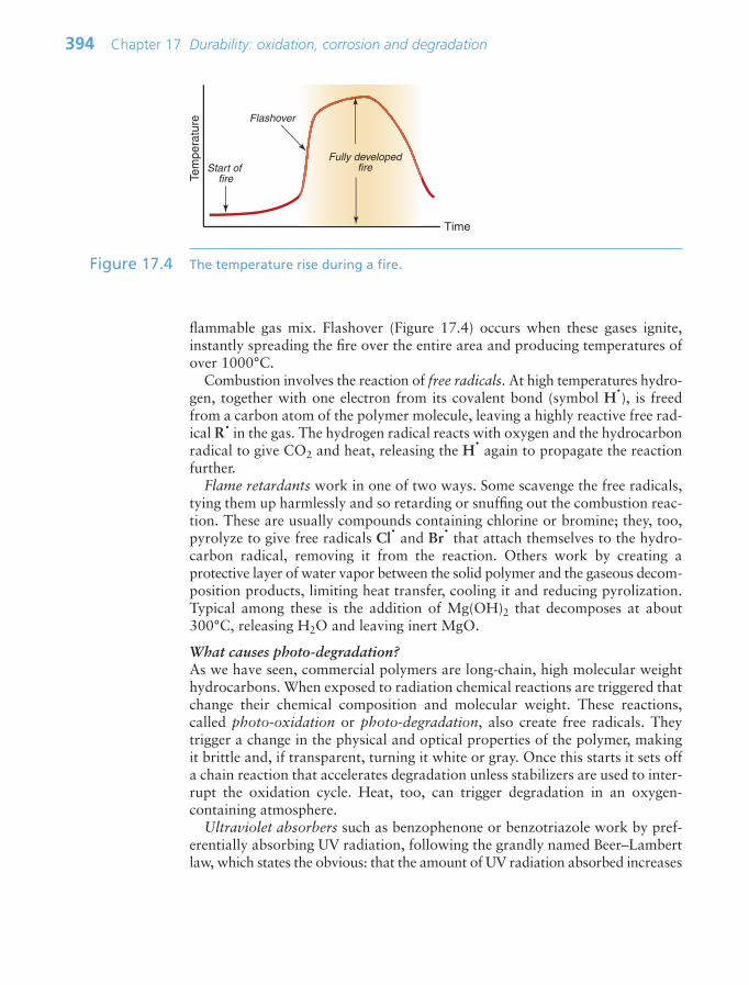
flammable gas mix. Flashover (Figure 17.4) occurs when these gases ignite,instantly spreading the fire over the entire area and producing temperatures ofover 1000°C.
Combustion involves the reaction of free radicals. At high temperatures hydro-gen, together with one electron from its covalent bond (symbol H), is freedfrom a carbon atom of the polymer molecule, leaving a highly reactive free rad-ical R in the gas. The hydrogen radical reacts with oxygen and the hydrocarbonradical to give CO2 and heat, releasing the H again to propagate the reactionfurther.
Flame retardants work in one of two ways. Some scavenge the free radicals,tying them up harmlessly and so retarding or snuffing out the combustion reac-tion. These are usually compounds containing chlorine or bromine; they, too,pyrolyze to give free radicals Cl and Br that attach themselves to the hydro-carbon radical, removing it from the reaction. Others work by creating aprotective layer of water vapor between the solid polymer and the gaseous decom-position products, limiting heat transfer, cooling it and reducing pyrolization.Typical among these is the addition of Mg(OH)2 that decomposes at about300°C, releasing H2O and leaving inert MgO.
What causes photo-degradation?As we have seen, commercial polymers are long-chain, high molecular weighthydrocarbons. When exposed to radiation chemical reactions are triggered thatchange their chemical composition and molecular weight. These reactions,called photo-oxidation or photo-degradation, also create free radicals. Theytrigger a change in the physical and optical properties of the polymer, makingit brittle and, if transparent, turning it white or gray. Once this starts it sets offa chain reaction that accelerates degradation unless stabilizers are used to inter-rupt the oxidation cycle. Heat, too, can trigger degradation in an oxygen-containing atmosphere.
Ultraviolet absorbers such as benzophenone or benzotriazole work by pref-erentially absorbing UV radiation, following the grandly named Beer–Lambertlaw, which states the obvious: that the amount of UV radiation absorbed increases
394 Chapter 17 Durability: oxidation, corrosion and degradation
Time
Tem
pera
ture
Start of fire
Flashover
Fully developedfire
Figure 17.4 The temperature rise during a fire.
Ch17-H8391.qxd 1/16/07 1:45 PM Page 394

with increase in the sample thickness and stabilizer concentration. In practice,high concentrations of absorbers and sufficient thickness of the polymer arerequired before enough absorption takes place to effectively retard photo-degra-dation. Hindered amine stabilizers (HALS) are a more efficient way to stabilizeagainst light-induced degradation of most polymers. They do not absorb UV radi-ation, but act to inhibit degradation of the polymer; their efficiency and longevityare due to a cyclic process wherein the HALS are regenerated rather than con-sumed. Low concentrations are enough to give good stabilization.
17.5 Corrosion: acids, alkalis, water and organic solvents
Acids, alkalis and aqueous liquidsStrong acids like H2SO4 (sulfuric acid), HNO3 (nitric acid) and HCl (hydrochlo-ric acid) are widely used in the chemical industry. So too are strong alkalis likeNaOH (caustic soda). Household products contain some of these in diluteform, but in the home it is organic acids like vinegar (acetic acid) and milderalkalis like washing soda (sodium carbonate) that are more commonly found.
Dunk a metal into an acid and you can expect trouble. The sulfates, nitrates,chlorides and acetates of most metals are more stable than the metal itself.Zinc, for instance, reacts with sulfuric acid, releasing hydrogen. The question isnot whether the metal will be attacked, but how fast. As with oxidation, thisdepends on the nature of the corrosion products and on any surface coating themetal may have. The oxide films on aluminum, titanium and chromium protectthem from some acids provided the oxide itself is not damaged.
Alkalis, too, attack some metals. Zinc, tin, lead and aluminum reactwith NaOH, for instance, to give zincates, stannites, plumbates and alumi-nates (as anyone who has heated washing soda in an aluminum pan will havediscovered).
Water is nearly as bad. Even when pure, water causes corrosion if oxygen isavailable. The rusting of steel alone presents enormous economic and reliabilityproblems. Corrosion, however, can be beautiful: the turquoise patina of copperon roofs and the deep browns of bronze statues are created by corrosion.
Organic solventsOrganic liquids are ubiquitous: we depend on them as fuels and lubricants, forcooking, for removing stains, as face cream, as nail varnish and much more.Any material in service will encounter them. Metals, ceramics and glasses arelargely immune to them, and some polymers can tolerate some organic liquidswithout problems. But not all.
Resistance to organic solvents, usually given as a ranking on a five-pointscale from Very bad to Very good, gives only the broadest indication of suscep-tibility. The identification of solvents that are incompatible with a given poly-mer is largely based on experience, trial and error, and intuition guided by suchrules as ‘like dissolves like’ and various definitions of solvent ‘strength’.
17.5 Corrosion: acids, alkalis, water and organic solvents 395
Ch17-H8391.qxd 1/16/07 1:45 PM Page 395
17.6 Drilling down: mechanisms of corrosion
Ions in solution and pHPure water, H2O, dissociates a little to give a hydrogen ion, H, and a hydroxylion, OH:
H2O ↔ H OH (17.6)
The product of the concentrations of the two ions is constant: increase one andthe other falls. This is known as the Law of Mass Action:
[H].[OH] constant (17.7)
where the square brackets mean ‘molar concentration’. In pure water there areequal numbers of the two types of ion, [H] [OH], and the value of theconstant, when measured, is 1014. Thus, the molar concentration of both iontypes is 107; one H2O molecule in 107 is ionized. The pH of the ionized wateris defined as the negative of the log of the hydrogen ion concentration:
pH log10[H] (17.8)
so, for pure water, pH 7.Acids dissociate in water to give H ions. Sulfuric acid, for instance, dissociates:
H2SO4 ↔ 2H SO42 (17.9)
This pushes up the concentration [H] and, because of equation (17.8), it pullsdown the concentration [OH]; weak acids have a pH of 4–6; strong ones a pHdown to 0. Alkalis do the opposite. Sodium hydroxide, for example, dissociateswhen dissolved in water, to give OH ions:
NaOH ↔ Na OH (17.10)
Weak alkalis have a pH of 8–10, strong ones a pH up to 13 (Figure 17.5).Corrosion by acids and alkalis is an electrochemical reaction. One-half of
this is the dissociation reaction of a metal M into a metal ion, Mz, releasingelectrons e:
where z, an integer of 1, 2 or 3, is the valence of the metal. Acidic environ-ments, with high [H] (and thus low pH) stimulate this reaction; thus, a metal such as copper, in sulfuric acid solution, reacts rapidly:
(17.11)Cu Cu 2e
H SO 2H SOCu SO
2
2 4 42
242
→
↔
⎫⎬⎪⎪⎪
⎭⎪⎪⎪
→ CuSO4
M M→ z ez
396 Chapter 17 Durability: oxidation, corrosion and degradation
Ch17-H8391.qxd 1/16/07 1:45 PM Page 396
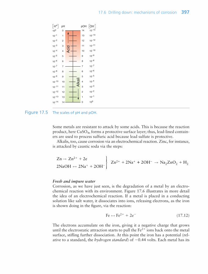
Some metals are resistant to attack by some acids. This is because the reactionproduct, here CuSO4, forms a protective surface layer; thus, lead-lined contain-ers are used to process sulfuric acid because lead sulfate is protective.
Alkalis, too, cause corrosion via an electrochemical reaction. Zinc, for instance,is attacked by caustic soda via the steps:
Fresh and impure waterCorrosion, as we have just seen, is the degradation of a metal by an electro-chemical reaction with its environment. Figure 17.6 illustrates in more detailthe idea of an electrochemical reaction. If a metal is placed in a conductingsolution like salt water, it dissociates into ions, releasing electrons, as the ironis shown doing in the figure, via the reaction:
Fe ↔ Fe2 2e (17.12)
The electrons accumulate on the iron, giving it a negative charge that growsuntil the electrostatic attraction starts to pull the Fe2 ions back onto the metalsurface, stifling further dissociation. At this point the iron has a potential (rel-ative to a standard, the hydrogen standard) of 0.44 volts. Each metal has its
Zn Zn 2e
2NaOH 2Na 2OHZn 2Na
22
→
↔
⎫⎬⎪⎪⎪
⎭⎪⎪⎪
2OH Na ZnO H2 2 2→
17.6 Drilling down: mechanisms of corrosion 397
0
1
2
3
4
5
6
7
8
9
10
11
12
13
14
Aci
d
Alk
ali
0
1
2
3
4
5
6
7
8
9
10
11
12
13
14
pH pOHH+ OH−
100
10−1
10−2
10−3
10−4
10−5
10−6
10−7
10−8
10−9
10−10
10−11
10−12
10−13
10−14 100
10−1
10−2
10−3
10−4
10−5
10−6
10−7
10−8
10−9
10−10
10−11
10−12
10−13
10−14
Figure 17.5 The scales of pH and pOH.
Ch17-H8391.qxd 1/16/07 1:45 PM Page 397
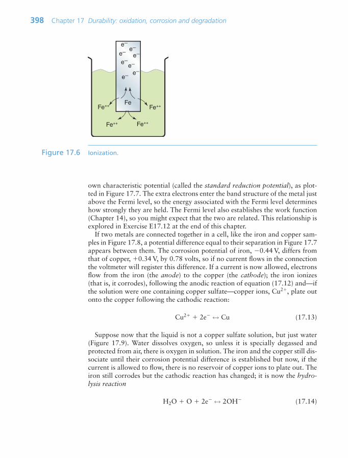
own characteristic potential (called the standard reduction potential), as plot-ted in Figure 17.7. The extra electrons enter the band structure of the metal justabove the Fermi level, so the energy associated with the Fermi level determineshow strongly they are held. The Fermi level also establishes the work function(Chapter 14), so you might expect that the two are related. This relationship isexplored in Exercise E17.12 at the end of this chapter.
If two metals are connected together in a cell, like the iron and copper sam-ples in Figure 17.8, a potential difference equal to their separation in Figure 17.7appears between them. The corrosion potential of iron, 0.44 V, differs fromthat of copper, 0.34 V, by 0.78 volts, so if no current flows in the connectionthe voltmeter will register this difference. If a current is now allowed, electronsflow from the iron (the anode) to the copper (the cathode); the iron ionizes(that is, it corrodes), following the anodic reaction of equation (17.12) and—ifthe solution were one containing copper sulfate—copper ions, Cu2, plate outonto the copper following the cathodic reaction:
Cu2 2e ↔ Cu (17.13)
Suppose now that the liquid is not a copper sulfate solution, but just water(Figure 17.9). Water dissolves oxygen, so unless it is specially degassed andprotected from air, there is oxygen in solution. The iron and the copper still dis-sociate until their corrosion potential difference is established but now, if thecurrent is allowed to flow, there is no reservoir of copper ions to plate out. Theiron still corrodes but the cathodic reaction has changed; it is now the hydro-lysis reaction
H2O O 2e ↔ 2OH (17.14)
398 Chapter 17 Durability: oxidation, corrosion and degradation
Fe Fe++ Fe++
Fe++ Fe++
e−e−
e−e−
e−
e−e−e−
Figure 17.6 Ionization.
Ch17-H8391.qxd 1/16/07 1:45 PM Page 398
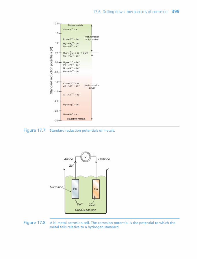
17.6 Drilling down: mechanisms of corrosion 399
Au Au+ + e−
Fe Fe++ + 2e−
Pt Pt++ + 2e−
Hg Hg++ + 2e−Ag Ag+ + e−
Cu Cu++ + 2e−
H2 2H+ + 2e−Pb Pb++ + 2e−
Ni Ni++ + 2e−
Cr Cr+++ + 3e−Zn Zn++ + 2e−
Al Al+++ + 3e−
Mg Mg++ + 2e−
Na Na+ + e−
H2O + O2 + 2e12 2 OH−
2.0
1.0
0.0
−1.0
−2.0
−3.0
1.5
0.5
−0.5
−1.5
−2.5
Sta
ndar
d re
duct
ion
pote
ntia
ls (
V)
Wet corrosionusual
Wet corrosionnot possible
Noble metals
Reactive metals
Figure 17.7 Standard reduction potentials of metals.
V− +
Fe
Fe++
2e−
2Cu+
CuSO4 solution
Corrosion
Anode Cathode
Cu
Figure 17.8 A bi-metal corrosion cell. The corrosion potential is the potential to which themetal falls relative to a hydrogen standard.
Ch17-H8391.qxd 1/16/07 1:45 PM Page 399

While oxygen can reach the copper, the corrosion reaction continues, creat-ing Fe2 ions at the anode and OH ions at the cathode. They react to forminsoluble Fe(OH)2, which ultimately oxidizes further to Fe2O3 H2O, rust.
Thus, connecting dissimilar metals in either pure water or water with dis-solved salts is a bad thing to do: corrosion cells appear that eat up the metalwith the lower (more negative) corrosion potential. Worse news is to come: itis not necessary to have two metals: both anodic and cathodic reactions cantake place on the same surface. Figure 17.10 shows how this happens. Here aniron sample is immersed in water with access to air. The part of the samplenearest the water surface has an easy supply of oxygen; that further away doesnot. On the remoter part the ionization reaction of equation (17.12) takes
400 Chapter 17 Durability: oxidation, corrosion and degradation
V− +
Fe
Fe++
2e−
2 OH−
O2 O2
Corrosion Cu
Anode Cathode
Figure 17.9 A bit-metal cell containing pure water in which oxygen can dissolve.
Fe
Fe++
4e
2OH−
O2 O2
Fe++
2OH−
Fe
Corrosion
Figure 17.10 A corrosion cell created by differential access to oxygen.
Ch17-H8391.qxd 1/16/07 1:45 PM Page 400
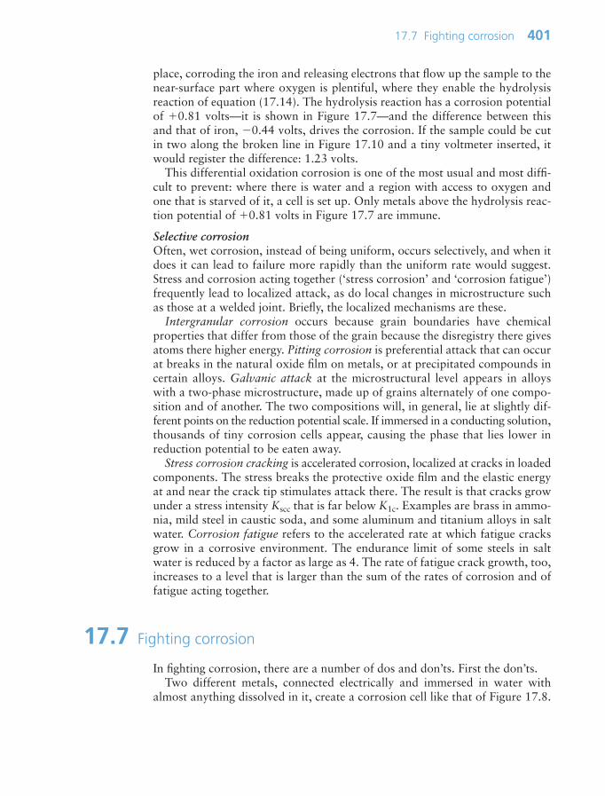
place, corroding the iron and releasing electrons that flow up the sample to thenear-surface part where oxygen is plentiful, where they enable the hydrolysisreaction of equation (17.14). The hydrolysis reaction has a corrosion potentialof 0.81 volts—it is shown in Figure 17.7—and the difference between thisand that of iron, 0.44 volts, drives the corrosion. If the sample could be cutin two along the broken line in Figure 17.10 and a tiny voltmeter inserted, itwould register the difference: 1.23 volts.
This differential oxidation corrosion is one of the most usual and most diffi-cult to prevent: where there is water and a region with access to oxygen andone that is starved of it, a cell is set up. Only metals above the hydrolysis reac-tion potential of 0.81 volts in Figure 17.7 are immune.
Selective corrosionOften, wet corrosion, instead of being uniform, occurs selectively, and when itdoes it can lead to failure more rapidly than the uniform rate would suggest.Stress and corrosion acting together (‘stress corrosion’ and ‘corrosion fatigue’)frequently lead to localized attack, as do local changes in microstructure suchas those at a welded joint. Briefly, the localized mechanisms are these.
Intergranular corrosion occurs because grain boundaries have chemicalproperties that differ from those of the grain because the disregistry there givesatoms there higher energy. Pitting corrosion is preferential attack that can occurat breaks in the natural oxide film on metals, or at precipitated compounds incertain alloys. Galvanic attack at the microstructural level appears in alloyswith a two-phase microstructure, made up of grains alternately of one compo-sition and of another. The two compositions will, in general, lie at slightly dif-ferent points on the reduction potential scale. If immersed in a conducting solution,thousands of tiny corrosion cells appear, causing the phase that lies lower inreduction potential to be eaten away.
Stress corrosion cracking is accelerated corrosion, localized at cracks in loadedcomponents. The stress breaks the protective oxide film and the elastic energyat and near the crack tip stimulates attack there. The result is that cracks growunder a stress intensity Kscc that is far below K1c. Examples are brass in ammo-nia, mild steel in caustic soda, and some aluminum and titanium alloys in saltwater. Corrosion fatigue refers to the accelerated rate at which fatigue cracksgrow in a corrosive environment. The endurance limit of some steels in saltwater is reduced by a factor as large as 4. The rate of fatigue crack growth, too,increases to a level that is larger than the sum of the rates of corrosion and offatigue acting together.
17.7 Fighting corrosion
In fighting corrosion, there are a number of dos and don’ts. First the don’ts.Two different metals, connected electrically and immersed in water with
almost anything dissolved in it, create a corrosion cell like that of Figure 17.8.
17.7 Fighting corrosion 401
Ch17-H8391.qxd 1/16/07 1:45 PM Page 401
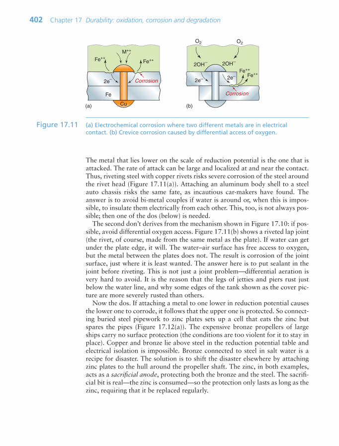
The metal that lies lower on the scale of reduction potential is the one that isattacked. The rate of attack can be large and localized at and near the contact.Thus, riveting steel with copper rivets risks severe corrosion of the steel aroundthe rivet head (Figure 17.11(a)). Attaching an aluminum body shell to a steelauto chassis risks the same fate, as incautious car-makers have found. Theanswer is to avoid bi-metal couples if water is around or, when this is impos-sible, to insulate them electrically from each other. This, too, is not always pos-sible; then one of the dos (below) is needed.
The second don’t derives from the mechanism shown in Figure 17.10: if pos-sible, avoid differential oxygen access. Figure 17.11(b) shows a riveted lap joint(the rivet, of course, made from the same metal as the plate). If water can getunder the plate edge, it will. The water–air surface has free access to oxygen,but the metal between the plates does not. The result is corrosion of the jointsurface, just where it is least wanted. The answer here is to put sealant in thejoint before riveting. This is not just a joint problem—differential aeration isvery hard to avoid. It is the reason that the legs of jetties and piers rust justbelow the water line, and why some edges of the tank shown as the cover pic-ture are more severely rusted than others.
Now the dos. If attaching a metal to one lower in reduction potential causesthe lower one to corrode, it follows that the upper one is protected. So connect-ing buried steel pipework to zinc plates sets up a cell that eats the zinc butspares the pipes (Figure 17.12(a)). The expensive bronze propellers of largeships carry no surface protection (the conditions are too violent for it to stay inplace). Copper and bronze lie above steel in the reduction potential table andelectrical isolation is impossible. Bronze connected to steel in salt water is arecipe for disaster. The solution is to shift the disaster elsewhere by attachingzinc plates to the hull around the propeller shaft. The zinc, in both examples,acts as a sacrificial anode, protecting both the bronze and the steel. The sacrifi-cial bit is real—the zinc is consumed—so the protection only lasts as long as thezinc, requiring that it be replaced regularly.
402 Chapter 17 Durability: oxidation, corrosion and degradation
Fe
Fe++ Fe++
2e−
M++
2OH−
O2 O2
2OH−
Corrosion
Fe++
Fe++
Corrosion
Cu
2e− 2e−
(a) (b)
Figure 17.11 (a) Electrochemical corrosion where two different metals are in electricalcontact. (b) Crevice corrosion caused by differential access of oxygen.
Ch17-H8391.qxd 1/16/07 1:45 PM Page 402
Plating can work in the same way. Galvanized iron is steel sheet with a thincoating of zinc. The zinc acts as a sacrificial anode (Figure 17.12(b)): ifscratched, the exposed steel does not rust because the zinc protects it even whenit does not cover it. Other platings look good but do not protect so well. A plat-ing of copper sets up a cell the works in the opposite direction, eating the ironat a scratch rather than the copper. Chromium plating looks as if it should pro-tect, since chromium is below iron in the table, but the chromium protects itselfso well with its oxide film that it becomes passive and no cell is set up. It is thispassivity that makes the stainless alloys described in Section 17.3 good at resist-ing aqueous corrosion as well. Stainless steel is not just oxidation resistant, it iscorrosion resistant too, and the same is true of the other alloys listed there.
When tricks like these cannot be used to prevent corrosion, the answer is toseparate the reactive metal from the corrosive medium with a polymer film.Painting with solvent-based paints was, until recently, the most widely usedmethod, but the evaporating solvent is generally toxic; it is a VOC (a volatileorganic compound) and, for health reasons, their use is discouraged. Water-based paints overcome the problem but do not yet produce quite as good apaint film. Polymer powder coating works by plasma-spraying the polymer ordipping the component when hot into a fluidized bed of polymer powder, caus-ing a thick film of polymer to melt onto the surface. While intact, paint filmsand polymer powder coats work well, but as soon as the coating is damagedthe protection ceases unless the underlying metal has a sub-coat of something—like zinc—that protects it.
Organic solvents and the solubility parameterOrganic solvents attack certain polymers. The nearest that this can be made sci-entific is via what are called solubility parameters. Polymer chains are bondedstrongly (covalent bonding) along their length, but only weakly (van der Waalsbonding) between chains. To enter a polymer the solvent, like a virus, musttrick these bonds into allowing them in—that is where the ‘like dissolves like’,
17.7 Fighting corrosion 403
Wet soil
4e−
O2 O2
4OH− Zn ++
Zn ++
V
Zn++ Zn++
4OH−
O2 O2
2e− 2e−
(a) (b)
Zn Zn
Steel sheetZinc
coating
Figure 17.12 (a) Protection of steel pipes by a zinc sacrificial anode. (b) Galvanized steelplate; the zinc protects the steel even when scratched.
Ch17-H8391.qxd 1/16/07 1:45 PM Page 403
mentioned earlier, comes from. Once in—like viruses—they do things: mostlybad, a few, good.
The bad: like UV radiation, aggressive solvents cause discoloration, reducestrength, induce brittleness and trigger crazing (the whitening of the polymerbecause of many tiny crack-like expansion cavities). The good: certain organicsolvents act as plasticizers, reducing the glass temperature but not the strength,converting a rigid polymer into a flexible, leather-like material. Artificialleather—plasticized PVC—is an example. Many plasticizers are phthalates butincreasing concern for their potential toxicity generates pressure to use alterna-tives. Increasingly they are replaced by biochemical plasticizers—vegetable oilssuch as soybean oil or linseed oil—although these are more expensive.
Which organic solvents are the worst? Not an easy question. Amyl acetate(nail varnish) is particularly aggressive, as is chloroform (anesthetics), but thisis no answer. To get a full answer you have to turn to the more specialized CESOPS database (which runs in the same system as that of the one used to makethe charts and for the exercises in this book); it gives detailed rankings of alarge number of individual polymers in a large number of different organic(and other) gases and liquids.
17.8 Summary and conclusions
Corrosion is like cancer: it will kill you unless something else (like wear) killsyou first. Almost as much money must have been invested in corrosion researchas in research on cancer, such is its damaging effect on the economy. This researchhas revealed what goes on at an atomic scale when materials react with oxygen,acids, alkalis, aqueous solutions, aerated water and organic solvents.
All involve electrochemical reactions or reactions involving free radicals. Inoxidation of metals, the metal ionizes, releasing electrons; the electrons com-bine with oxygen molecules to give oxygen ions, that in turn combine withmetal ions to form the oxide. As the oxide film grows, ions and electrons mustdiffuse through it to enable further growth; its resistance to this diffusion, andits ability to adhere to the metal surface, determine how protective it is. Polymersoxidize through the action of free radicals. Radiation, including UV light, cangenerate the free radicals, as does heat. Polymers are protected by doping themwith UV filters and with additions that absorb free radicals.
In corrosion, the electrochemical reactions occur in the corrosive fluid ratherthan in the solid. A metal ionizes when placed in water. The extent of ioniza-tion determines its reduction potential. Those with the smallest (most negative)reduction potential are the most vulnerable to attack and will corrode sponta-neously, even in pure water if oxygen is present. If a metal with a low reductionpotential is in electrical contact with one of higher potential, the first corrodesand the second is protected.
In designing materials to resist corrosion we rely on the ability of a few ofthem—chromium, aluminum, silicon and titanium—to form a protective oxide
404 Chapter 17 Durability: oxidation, corrosion and degradation
Ch17-H8391.qxd 1/16/07 1:45 PM Page 404
film that adheres strongly to the surface. By using these as alloying elements,other metals can be given the same protection. Alternatively, metals can be pro-tected by coating their surfaces with a corrosion-resistant film of polymer orceramic.
17.9 Further reading
Bradford, S.A. (1993) Corrosion Control, Van Nostrand Reinhold, New York, USA.ISBN 0-442-01088-5. (A text emphasizing practical ways of preventing or dealingwith corrosion.)
Fontanta, M.G. (1986) Corrosion Engineering, 3rd edition, McGraw-Hill, New York,USA. ISBN 0-07-021463-8. (A text focusing on the practicalities of corrosionengineering rather than the science, with numerous examples and data.)
Schweitzer, P.A. (1995) Corrosion Resistance Tables, 4th edition, Volumes 1–3, MarcelDekker, New York, USA. (The ultimate compilation of corrosion data in numerousenvironments. Not bedtime reading.)
Schweitzer, P.A. (1998) Encyclopedia of Corrosion Technology, Marcel Dekker, NewYork, USA. ISBN 0-8247-0137-2. (A curious compilation, organized alphabetically,that mixes definitions and terminology with tables of data.)
Tretheway, K.R. and Chamberlain, J. (1995) Corrosion for Science and Engineering,2nd edition, Longman Scientific and Technical, Harlow, UK. ISBN 0-582-238692.(An unusually readable introduction to corrosion science, filled with little benchtopexperiments to illustrate principles.)
Waterman, N.A. and Ashby, M.F. (1991) Elsevier Materials Selector, Elsevier, Oxford,UK. ISBN 1-85-166-605-2 and, in the CRC edition, ISBN 0-8493-7790-0. (A three-volume compilation of materials data for design, with extensive tables and guidelinesfor the oxidation and corrosion characteristics of metals and polymers.)
17.10 Exercises 405
17.10 Exercises
Exercise E17.1 By what mechanisms do metals oxidize? What determines the rate of oxidation?
Exercise E17.2 The oxidation kinetics of titanium to TiO2 is limited by oxygen diffusion,with an activation energy Qd of 275 kJ/mol. If the oxide film grows to athickness of 0.08 µm after 1 hour at 800°C, how thick a film would youexpect if it had been grown at 1000°C for 30 minutes?
Exercise E17.3 What is meant by the standard reduction potential? A copper and a platinumelectrode are immersed in a bath of dilute copper sulfate. What potential dif-ference would you expect to measure between them? If they are connected sothat a current can flow, which one will corrode?
Ch17-H8391.qxd 1/16/07 1:45 PM Page 405

406 Chapter 17 Durability: oxidation, corrosion and degradation
17.11 Exploring design with CES (use Level 2 unlessotherwise stated)
Exercise E17.4 Find, by browsing or searching, the record for the nickel–chromium alloyscalled nichromes. What are their main applications?
Exercise E17.5 Find, by browsing or searching, the record for polymer powder coating(remember to search in the Process Universe, not the Materials Universe).What are the three ways of applying a polymer powder coating?
Exercise E17.6 Use a ‘Limit’ stage, applied to the Level 2 Surface Treatment data table, tofind surface treatment processes that impart resistance to gaseous corrosion.
Exercise E17.7 Use a ‘Limit’ stage, applied to the Level 2 Surface Treatment data table to findsurface treatment processes that impart resistance to aqueous corrosion.
Exercise E17.8 Use the CES ‘Search’ facility to find materials for food processing equipment.
Exercise E17.9 Plastic cases for electrical plugs and switch-gear should not be made of flam-mable materials. Use the ‘Select’ facility in CES to find polymers that arenon-flammable or self-extinguishing.
Exercise E17.10 A vat is required to hold hot caustic soda, NaOH, a strong alkali. Use the‘Select’ facility in CES to find metals that resist strong alkalis very well.
Exercise E17.11 Pipework is required for a gherkin-pickling plant to carry vinegar (a weakacid) at 100°C from one vat to another. The liquid is under pressure, requir-ing a material with a strength of at least 100 MPa, and for ease of installa-tion it must be able to be bent, requiring a ductility of at least 10%. Find thefour cheapest materials that meet the constraints, summarized below.
Function • Pipework for hot acetic acid
Constraints • Durability in weak acid very good
• Maximum operating temperature 100°C
• Yield strength 100 MPa
• Elongation 10%
Objective • Minimize material price
Free variable • Choice of material
Ch17-H8391.qxd 1/16/07 1:45 PM Page 406

17.12 Exploring the science with CES Elements 407
Exercise E17.12 The work function (Chapter 14) is the energy required to pluck an electronfrom the top of the Fermi level of a crystal and drag it away until it is iso-lated in vacuum. The standard reduction potential of Figure 17.7 involveselectrons dropping into energy levels just above the Fermi level. You mightsuspect that the two were, in some way, related. Make a graph with stan-dard reduction potential on the x-axis and work function on the y-axis tofind out if they are. What is your conclusion?
17.12 Exploring the science with CES Elements
Ch17-H8391.qxd 1/16/07 1:45 PM Page 407

This page intentionally left blank
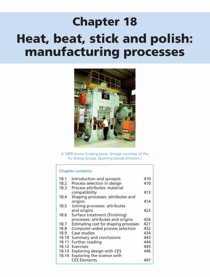
Chapter 18Heat, beat, stick and polish:
manufacturing processes
Chapter contents
18.1 Introduction and synopsis 41018.2 Process selection in design 41018.3 Process attributes: material
compatibility 41318.4 Shaping processes: attributes and
origins 41418.5 Joining processes: attributes
and origins 42318.6 Surface treatment (finishing)
processes: attributes and origins 42618.7 Estimating cost for shaping processes 42718.8 Computer-aided process selection 43218.9 Case studies 43418.10 Summary and conclusions 44318.11 Further reading 44418.12 Exercises 44518.13 Exploring design with CES 44618.14 Exploring the science with
CES Elements 447
A 1000 tonne forging press. (Image courtesy of the Fu Sheng Group, Sporting Goods Division.)
Ch18-H8391 1/16/07 6:43 PM Page 409

410 Chapter 18 Heat, beat, stick and polish: manufacturing processes
18.1 Introduction and synopsis
Materials and processing are inseparable. Ores, minerals and oil are processedto create the stuff of engineering in clean, usable form. These are shaped intocomponents, finished and joined to make products. Chapter 3 defined a hierar-chy for these processes; in this chapter we explore their technical capabilitiesand methods for choosing which to use. Increasingly, legislation and publicopinion require that materials are recycled at the end of product life. Newprocesses are emerging to extract usable material from what used to be regardedas waste.
The strategy for choosing a process parallels that for materials: screen outthose that cannot do the job, rank those that can (usually seeking those with thelowest cost) and explore the documented knowledge of the top-ranked candi-dates. Many technical characteristics of a process can be described by numericand non-numeric data: the size of part it can produce, the surface finish of whichit is capable and, critically, the material families or classes it can handle and theshapes it can make. Constraints on these provide the inputs for screening, givinga short list of processes that meet the requirements of the design.
There is another aspect to this. It relates to the influence of processing on theproperties of the materials themselves. Materials, of course, have properties beforethey are shaped, joined or finished and processing is used to enhance propertiessuch as strength. But the act of processing can also damage properties by intro-ducing porosity, cracks and defects or by changing the microstructure in a detri-mental way. These interactions, central to the choice and control of processes, areexplored further in Chapter 19. For now, it is sufficient to recognize that successin manufacturing often relies on accumulated know-how and expertise, resident,in the past, in the heads of long-established employees but now captured asdesign guidelines, best practice guides and software providing the informationneeded for the documentation stage.
18.2 Process selection in design
The selection strategyThe taxonomy of manufacturing processes was presented in Chapter 2. There,it was established that processes fall into three broad families: shaping, joiningand finishing (Figures 2.4 and 2.5). Each is characterized by a set of attributeslisted, in part, in Figures 2.6 and 2.7.
The strategy for materials selection was outlined in Chapter 3. The proce-dure, whether dealing with original design or refining an existing one, was totranslate the design requirements into a set of constraints and objectives. Theconstraints are used to screen and the objectives to rank, delivering a preferredshort-list of materials that best meet both, finally seeking documentation toguide the final choice. The strategy for selecting processes follows a parallel
Ch18-H8391 1/16/07 6:43 PM Page 410
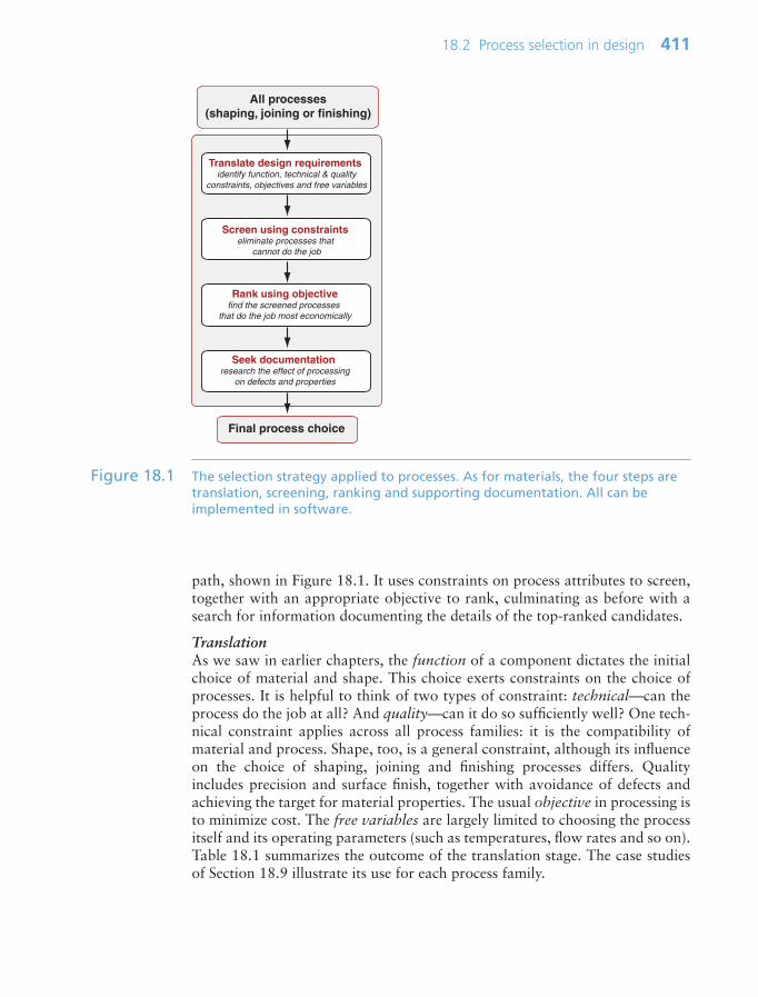
18.2 Process selection in design 411
path, shown in Figure 18.1. It uses constraints on process attributes to screen,together with an appropriate objective to rank, culminating as before with asearch for information documenting the details of the top-ranked candidates.
TranslationAs we saw in earlier chapters, the function of a component dictates the initialchoice of material and shape. This choice exerts constraints on the choice ofprocesses. It is helpful to think of two types of constraint: technical—can theprocess do the job at all? And quality—can it do so sufficiently well? One tech-nical constraint applies across all process families: it is the compatibility ofmaterial and process. Shape, too, is a general constraint, although its influenceon the choice of shaping, joining and finishing processes differs. Qualityincludes precision and surface finish, together with avoidance of defects andachieving the target for material properties. The usual objective in processing isto minimize cost. The free variables are largely limited to choosing the processitself and its operating parameters (such as temperatures, flow rates and so on).Table 18.1 summarizes the outcome of the translation stage. The case studiesof Section 18.9 illustrate its use for each process family.
Translate design requirements identify function, technical & quality
constraints, objectives and free variables
All processes(shaping, joining or finishing)
Final process choice
Screen using constraints eliminate processes that
cannot do the job
Rank using objectivefind the screened processes
that do the job most economically
Seek documentation research the effect of processing
on defects and properties
Figure 18.1 The selection strategy applied to processes. As for materials, the four steps aretranslation, screening, ranking and supporting documentation. All can beimplemented in software.
Ch18-H8391 1/16/07 6:43 PM Page 411
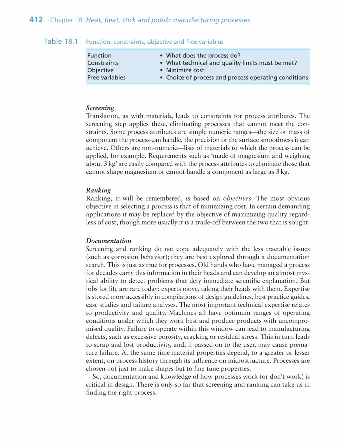
ScreeningTranslation, as with materials, leads to constraints for process attributes. Thescreening step applies these, eliminating processes that cannot meet the con-straints. Some process attributes are simple numeric ranges—the size or mass ofcomponent the process can handle, the precision or the surface smoothness it canachieve. Others are non-numeric—lists of materials to which the process can beapplied, for example. Requirements such as ‘made of magnesium and weighingabout 3 kg’ are easily compared with the process attributes to eliminate those thatcannot shape magnesium or cannot handle a component as large as 3 kg.
RankingRanking, it will be remembered, is based on objectives. The most obviousobjective in selecting a process is that of minimizing cost. In certain demandingapplications it may be replaced by the objective of maximizing quality regard-less of cost, though more usually it is a trade-off between the two that is sought.
DocumentationScreening and ranking do not cope adequately with the less tractable issues(such as corrosion behavior); they are best explored through a documentationsearch. This is just as true for processes. Old hands who have managed a processfor decades carry this information in their heads and can develop an almost mys-tical ability to detect problems that defy immediate scientific explanation. Butjobs for life are rare today; experts move, taking their heads with them. Expertiseis stored more accessibly in compilations of design guidelines, best practice guides,case studies and failure analyses. The most important technical expertise relatesto productivity and quality. Machines all have optimum ranges of operatingconditions under which they work best and produce products with uncompro-mised quality. Failure to operate within this window can lead to manufacturingdefects, such as excessive porosity, cracking or residual stress. This in turn leadsto scrap and lost productivity, and, if passed on to the user, may cause prema-ture failure. At the same time material properties depend, to a greater or lesserextent, on process history through its influence on microstructure. Processes arechosen not just to make shapes but to fine-tune properties.
So, documentation and knowledge of how processes work (or don’t work) iscritical in design. There is only so far that screening and ranking can take us infinding the right process.
412 Chapter 18 Heat, beat, stick and polish: manufacturing processes
Function • What does the process do?Constraints • What technical and quality limits must be met?Objective • Minimize costFree variables • Choice of process and process operating conditions
Table 18.1 Function, constraints, objective and free variables
Ch18-H8391 1/16/07 6:43 PM Page 412

18.3 Process attributes: material compatibility
The main goal in defining process attributes is to identify the characteristicsthat discriminate between processes, to enable their selection by screening.Each of the three process families—shaping, joining and surface treatment—has it own set of characterizing attributes, described here and in the next threesections. It is also of interest to explore the physical limits to these for a givenprocess, and to examine how the properties of the material being processedlimit the rate of the process itself.
One process attribute applies to all three families—compatibility with material—so we examine this first.
Material–process compatibilityFigure 18.2 shows a material–process compatibility matrix. Shaping processesare at the top, with compatible combinations marked by dots the color ofwhich identifies the material family. Its use for screening is straightforward—specify the material and some processes are immediately eliminated (or thereverse, as a screening step in material selection). The diagonal spread of thedots in the matrix reveals that each material class—metals, polymers, etc.—hasits own set of process routes. This largely reflects the underlying processphysics. Shaping is usually eased by melting or softening the material, and themelting temperatures of the material classes are quite distinct (Figure 13.6).There are some overlaps—powder methods are compatible with both metalsand ceramics, molding with both polymers and glasses. Machining (when usedfor shaping) is compatible with almost all families. Joining processes usingadhesives and fasteners are very versatile and can be used with most materials,whereas welding methods are material specific. Finishing processes are prima-rily used for the harder materials, particularly metals—polymers are molded toshape and rarely treated further except for decorative purposes. We will seewhy later.
Coupling of material selection and process selectionThe choice of material and of process are clearly linked. The compatibility matrixshows that the choice of material isolates a sub-domain of processes. The processchoice feeds back to material selection. If, say, aluminum alloys were chosen inthe initial material selection stage and casting in the initial process selection stage,then only the subset of aluminum alloys that are castable can be used. If the com-ponent is then to be age hardened (a heat-treatment process), material choice isfurther limited to heat-treatable aluminum casting alloys. So we must continuallyiterate between process and material, checking that inconsistent combinationsare avoided. The key point is that neither material nor process choice can be car-ried too far without giving thought to the other. Once past initial screening, it isessentially a co-selection procedure.
18.3 Process attributes: material compatibility 413
Ch18-H8391 1/16/07 6:43 PM Page 413

18.4 Shaping processes: attributes and origins
Mass and section thicknessThere are limits to the size of component that a process can make. Figure 18.3shows the limits. The color coding for material compatibility has been retained,using more than one color when the process can treat more than one materialfamily. Size can be measured by volume or by mass, but since the range of eitherone covers many orders of magnitude, while densities only span a factor ofabout 10, it doesn’t make much difference which we use—big things are heavy,
414 Chapter 18 Heat, beat, stick and polish: manufacturing processes
Cer
amic
s
Gla
sses
Met
als,
ferr
ous
Met
als,
non
-fer
rous
The
rmop
last
ics
Ela
stom
ers
The
rmos
ets
Com
posi
tes
Pol
ymer
foam
s
Sand castingDie casting
Investment casting
ForgingExtrusion
Sheet formingPowder methods
Conventional machiningInjection molding
Blow moldingCompression molding
Rotational molding
Polymer casting
Filament winding
Low-pressure casting
Thermo-forming
Lay-up methodsVacuum bag
Resin-transfer molding
Electro-machining
Polishing
Fini
shin
g
GrindingLapping
Precision machining
Adhesives
Fasteners
Join
ing
Welding, metalsWelding, polymers
Sha
ping
metal ceramic polymer composite foam
Spark plug
CDcase
Con- rod
Con- rod
Figure 18.2 The material–process compatibility matrix for shaping, joining and finishingprocesses color coded by material. Ignore the boxes on first reading; they referto case studies to come.
Ch18-H8391 1/16/07 6:43 PM Page 414

whatever they are made of. Most processes span a mass range of about a factorof 1000 or so. Note that this attribute is most discriminating at the extremes;the vast majority of components are in the 0.1–10 kg range, for which virtuallyany process will work.
It is worth noting what the ranges represent. Each bar spans the size range ofwhich the process is capable without undue technical difficulty. All can bestretched to smaller or larger extremes but at the penalty of extra cost becausethe equipment is no longer standard. During screening, therefore, it is importantto recognize ‘near misses’—processes which narrowly failed, but which could, ifneeded, be reconsidered and used.
Figure 18.4 shows a second bar chart: that for the ranges of section thicknessof which each shaping process is capable. It is the lower end of the ranges—theminimum section thickness—where the physics of the process imposes limits.Their origins are the subject of the next sub-section.
Physical limits to size and section thicknessCasting and molding both rely on material flow in the liquid or semi-liquidstate. Lower limits on section thickness are imposed by the physics of flow.
18.4 Shaping processes: attributes and origins 415
10−3 10−2 0.1 1 10 102 103 104
Mass (kg)
Sand castingDie casting
Investment Casting
ForgingExtrusion
Sheet formingPowder methods
Conventional machiningInjection molding
Blow moldingCompression molding
Rotational molding
Polymer casting
Filament winding
Low-pressure casting
Thermo-forming
Lay-up methodsVacuum bag
Resin-transfer molding
Electro-machining
Met
al s
hapi
ng
Cer
amic
shap
ing
Pol
ymer
shap
ing
Com
posi
te s
hapi
ng
Spark plug
CDcase
Con- rod
metal ceramic polymer composite
Figure 18.3 The process–mass range bar chart for shaping processes. Ignore, on firstreading, the boxes; they refer to case studies to come. The colors refer to thematerial, as in Figure 18.2. Multiple colors indicate compatibility with more thanone family.
Ch18-H8391 1/16/07 6:43 PM Page 415
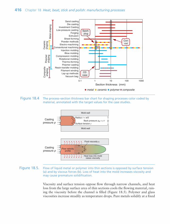
Viscosity and surface tension oppose flow through narrow channels, and heatloss from the large surface area of thin sections cools the flowing material, rais-ing the viscosity before the channel is filled (Figure 18.5). Polymer and glass viscosities increase steadily as temperature drops. Pure metals solidify at a fixed
416 Chapter 18 Heat, beat, stick and polish: manufacturing processes
Section thickness (mm)
0.1 1 10 100 1000
Sand castingDie casting
Investment Casting
ForgingExtrusion
Sheet formingPowder methods
Conventional machiningInjection molding
Blow moldingCompression molding
Rotational molding
Polymer casting
Filament winding
Low-pressure casting
Thermo-forming
Lay-up methodsVacuum bag
Resin-transfer molding
Electro-machining
Met
al s
hapi
ng
Cer
amic
shap
ing
Pol
ymer
shap
ing
Com
posi
te s
hapi
ng
Spark plug
CDcase
Con- rod
metal ceramic polymer composite
Figure 18.4 The process–section thickness bar chart for shaping processes color coded bymaterial, annotated with the target values for the case studies.
Mold wall
Mold wall
Radius r = w/2Back pressure ps = γ/r
Surface tension γ
Heat loss into moldraises viscosity
w
Fluid viscosity η
Flow velocityprofile
Castingpressure p
Castingpressure p
Figure 18.5. Flow of liquid metal or polymer into thin sections is opposed by surface tension(a) and by viscous forces (b). Loss of heat into the mold increases viscosity andmay cause premature solidification.
Ch18-H8391 1/16/07 6:43 PM Page 416

temperature, with a step increase in viscosity, but for alloys this happens over arange of temperature, known as the ‘mushy zone’, in which the alloy is part liq-uid, part solid. The width of this zone can vary from a few degrees centigradeto several hundred—so metal flow in castings depends on alloy composition.In general, higher pressure die-casting and molding methods enable thinner sections to be made, but the equipment costs more and the faster, more turbu-lent flow can entrap more porosity and cause damage to the molds.
Upper limits to size and section in casting and molding are set by problemsof shrinkage. The outer layer of a casting or molding cools and solidifies first,giving it a rigid skin. When the interior subsequently solidifies, the change involume can distort the product or crack the skin, or cause internal cavitation.Problems of this sort are most severe where there are changes of section, sincethe constraint introduces tensile stresses that cause hot tearing—crackingcaused by constrained thermal contraction. Different compositions have differ-ent susceptibilities to hot tearing—another example of coupling between mate-rial, process and design detail.
Much of the documentation for casting and molding processes concernsguidance on designing both the component shape and the mold geometry toachieve the desired cross-sections while avoiding defects. Even when the com-ponent shape is fixed, there is freedom to choose where the material inlets arebuilt into the mold (the ‘runners’) and where the air and excess material willescape (the ‘risers’). Figure 18.6 shows an example of good practice in design-ing the cross-sectional shape of a polymer molding.
Powder methods for metals and ceramics too depend on flow. Filling a moldwith powder uses free flow under gravity plus vibration to bed the powderdown and achieve uniform filling. This may be followed by compression (‘coldcompaction’). Once full of powder, the mold is heated to allow densification bysintering or, if the pressure is maintained, by hot isostatic pressing (HIPing).
Metal shaping by deformation—hot or cold rolling, forging or extrusion—alsoinvolves flow. Solid metals flow by plastic deformation or by creep—Chapter 13described how the flow rate depends on stress and temperature. Much forming
18.4 Shaping processes: attributes and origins 417
Tension causedby differential
shrinkage
More uniformcross-section
avoids problem
Figure 18.6 (a) Differential shrinkage causes internal stress, distortion and cavitation in thicksections or at changes of section. (b) Good design keeps section thickness asuniform as possible, avoiding the problem.
Ch18-H8391 1/16/07 6:43 PM Page 417
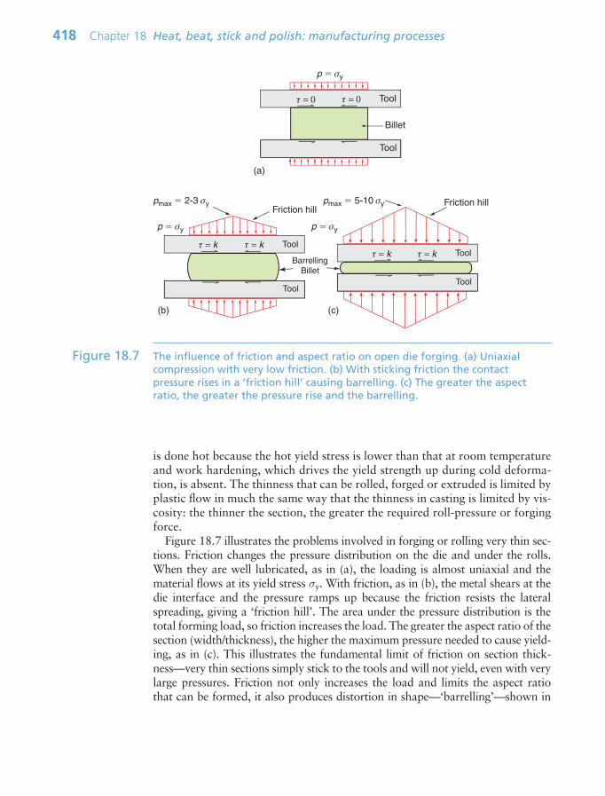
is done hot because the hot yield stress is lower than that at room temperatureand work hardening, which drives the yield strength up during cold deforma-tion, is absent. The thinness that can be rolled, forged or extruded is limited byplastic flow in much the same way that the thinness in casting is limited by vis-cosity: the thinner the section, the greater the required roll-pressure or forgingforce.
Figure 18.7 illustrates the problems involved in forging or rolling very thin sec-tions. Friction changes the pressure distribution on the die and under the rolls.When they are well lubricated, as in (a), the loading is almost uniaxial and thematerial flows at its yield stress σy. With friction, as in (b), the metal shears at thedie interface and the pressure ramps up because the friction resists the lateralspreading, giving a ‘friction hill’. The area under the pressure distribution is thetotal forming load, so friction increases the load. The greater the aspect ratio of thesection (width/thickness), the higher the maximum pressure needed to cause yield-ing, as in (c). This illustrates the fundamental limit of friction on section thick-ness—very thin sections simply stick to the tools and will not yield, even with verylarge pressures. Friction not only increases the load and limits the aspect ratio that can be formed, it also produces distortion in shape—‘barrelling’—shown in
418 Chapter 18 Heat, beat, stick and polish: manufacturing processes
Tool
Tool
p σy
p σyp σy
Billet
(a)
Tool
Tool
Friction hill
(c)
Tool
Tool
Friction hill
(b)
BarrellingBillet
pmax 5-10 σypmax 2-3 σy
τ = 0
τ = kτ = k τ = k
τ = k
τ = 0
Figure 18.7 The influence of friction and aspect ratio on open die forging. (a) Uniaxialcompression with very low friction. (b) With sticking friction the contactpressure rises in a ‘friction hill’ causing barrelling. (c) The greater the aspectratio, the greater the pressure rise and the barrelling.
Ch18-H8391 1/16/07 6:43 PM Page 418

both (b) and (c). A positive aspect of the high contact pressures in forging is therepeatability with which the metal can be forced to take up small featuresmachined on the face of the tooling, exploited in making coins.
Very small or very thin objects—pushing the limitsSo how do you make very small things? The obvious way to do it is to cut themout of bigger ones. That means machining: turning, shaping, drilling and milling.The upper limit on size is set by the budget available to buy the machine and theelectricity bill for its use. Lower limits—now we are thinking of milligrams andfractions of a millimeter—are set by the stiffness of the machine and the materialitself.
One continuous shaping process, rolling, is able to produce sections as thinas 10 µm—the thickness of aluminum kitchen foil. The foil only yields andthins just as it enters and leaves the roll bite—in between, the huge aspect ratioand frictional constraint mean that the high pressure actually flattens the steelrolls elastically. The process is helped by ‘pack rolling’—feeding two sheetsthrough together, with lubricant in between so that they can be peeled apart asthey exit the rolls. This is why kitchen foil is shiny on one side (where contactwas with the roll) and matt on the other.
Suppose you want to go still smaller. Flow won’t work, and the sections areso thin that they simply bend if you try to machine them. Now you need chem-istry. Conventional chemistry—etching, chemical milling, electro-dischargemilling—allow features on the same scale as that of precision machining. To getreally small, we need the screening, printing and etching techniques used to fab-ricate electronic devices. These are used to make MEMS (micro-electro-mechan-ical systems) — tiny sensors, actuators, gears and even engines. At present therange of materials is limited by this silicon-based technology, but some commer-cial devices, such as the inertial triggers for airbags, are made in this way.
ShapeA key attribute of a process is the families of shapes it can make. It is also oneof the most difficult to characterize. A classification scheme is illustrated inFigure 18.8, with three generic classes of shape, each sub-divided in two. Themerit of this approach is that processes map onto specific shapes. Figure 18.9shows the matrix of viable combinations.
The prismatic shapes shown on the left of Figure 18.8, made by rolling,extrusion or drawing, have a special feature: they can be made in continuouslengths. The other shapes cannot—they are discrete, and the processes thatmake them are called batch processes. The distinction between continuous anddiscrete (or batch) processes is a useful one, bearing on the cost of manufacture.Batch processes require repeated cycles of setting-up, which can be time-consuming and costly. On the other hand, they are often net-shape or nearly so,meaning that little further machining is needed to finish the component.Casting and molding processes are near net-shape. Forging, on the other hand,is limited by the strains and shape changes by solid-state plasticity, starting
18.4 Shaping processes: attributes and origins 419
Ch18-H8391 1/16/07 6:43 PM Page 419
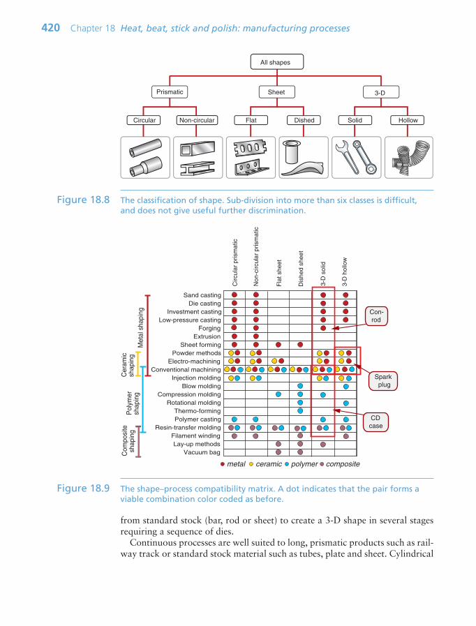
from standard stock (bar, rod or sheet) to create a 3-D shape in several stagesrequiring a sequence of dies.
Continuous processes are well suited to long, prismatic products such as rail-way track or standard stock material such as tubes, plate and sheet. Cylindrical
420 Chapter 18 Heat, beat, stick and polish: manufacturing processes
Prismatic Sheet 3-D
All shapes
Flat Dished Solid HollowCircular Non-circular
Figure 18.8 The classification of shape. Sub-division into more than six classes is difficult,and does not give useful further discrimination.
Sand castingDie casting
Investment casting
ForgingExtrusion
Sheet formingPowder methods
Conventional machiningInjection molding
Blow moldingCompression molding
Rotational molding
Polymer casting
Filament winding
Low-pressure casting
Thermo-forming
Lay-up methodsVacuum bag
Met
al s
hapi
ng
Cer
amic
shap
ing
Pol
ymer
shap
ing
Com
posi
te s
hapi
ng Resin-transfer molding
Electro-machining
Circ
ular
pris
mat
ic
Non
-circ
ular
pris
mat
ic
Fla
t she
et
Dis
hed
shee
t
3-D
sol
id
3-D
hol
low
Spark plug
CDcase
Con- rod
metal ceramic polymer composite
Figure 18.9 The shape–process compatibility matrix. A dot indicates that the pair forms aviable combination color coded as before.
Ch18-H8391 1/16/07 6:43 PM Page 420
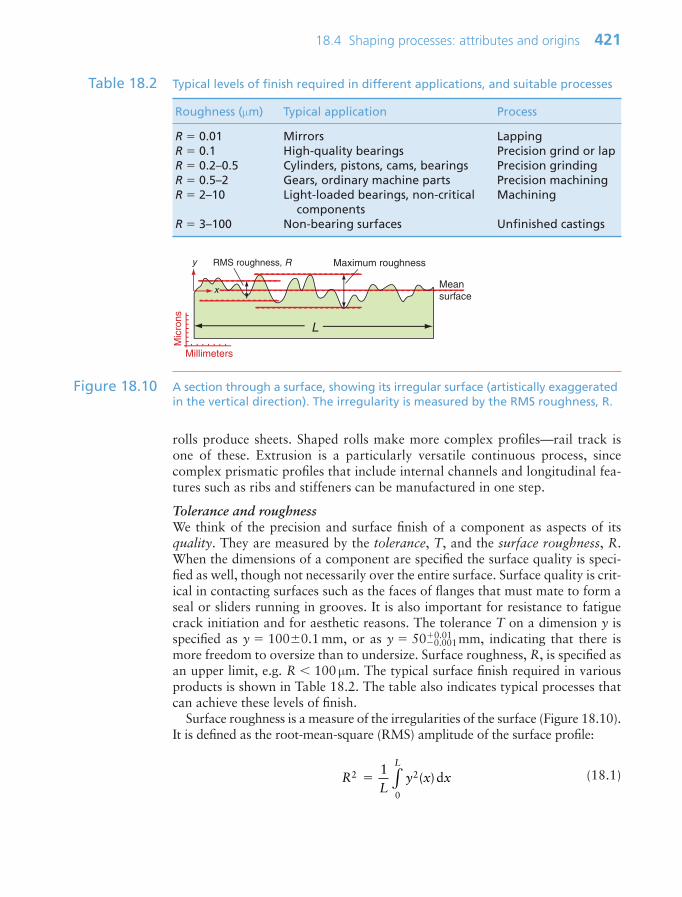
rolls produce sheets. Shaped rolls make more complex profiles—rail track isone of these. Extrusion is a particularly versatile continuous process, sincecomplex prismatic profiles that include internal channels and longitudinal fea-tures such as ribs and stiffeners can be manufactured in one step.
Tolerance and roughnessWe think of the precision and surface finish of a component as aspects of itsquality. They are measured by the tolerance, T, and the surface roughness, R.When the dimensions of a component are specified the surface quality is speci-fied as well, though not necessarily over the entire surface. Surface quality is crit-ical in contacting surfaces such as the faces of flanges that must mate to form aseal or sliders running in grooves. It is also important for resistance to fatiguecrack initiation and for aesthetic reasons. The tolerance T on a dimension y isspecified as y 1000.1 mm, or as y 500.01
0.001mm, indicating that there ismore freedom to oversize than to undersize. Surface roughness, R, is specified asan upper limit, e.g. R 100 µm. The typical surface finish required in variousproducts is shown in Table 18.2. The table also indicates typical processes thatcan achieve these levels of finish.
Surface roughness is a measure of the irregularities of the surface (Figure 18.10).It is defined as the root-mean-square (RMS) amplitude of the surface profile:
(18.1)RL
y x xL
2 2
0
1d ∫ ( )
18.4 Shaping processes: attributes and origins 421
Roughness (µm) Typical application Process
R 0.01 Mirrors LappingR 0.1 High-quality bearings Precision grind or lapR 0.2–0.5 Cylinders, pistons, cams, bearings Precision grindingR 0.5–2 Gears, ordinary machine parts Precision machiningR 2–10 Light-loaded bearings, non-critical Machining
componentsR 3–100 Non-bearing surfaces Unfinished castings
Table 18.2 Typical levels of finish required in different applications, and suitable processes
Mean surface
Maximum roughnessRMS roughness, R
x
y
Mic
rons
Millimeters
L
Figure 18.10 A section through a surface, showing its irregular surface (artistically exaggeratedin the vertical direction). The irregularity is measured by the RMS roughness, R.
Ch18-H8391 1/16/07 6:43 PM Page 421
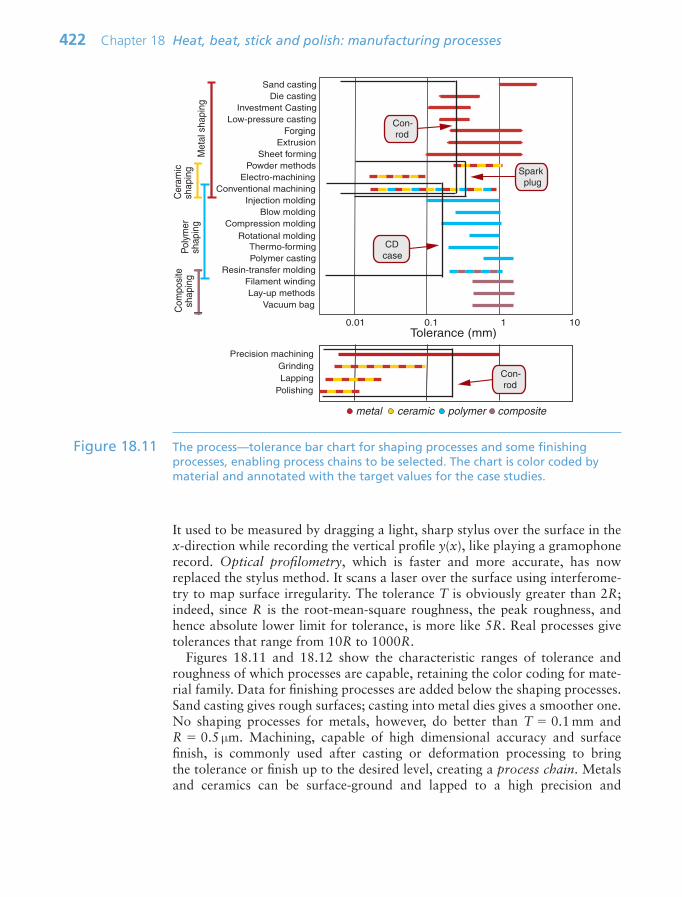
It used to be measured by dragging a light, sharp stylus over the surface in thex-direction while recording the vertical profile y(x), like playing a gramophonerecord. Optical profilometry, which is faster and more accurate, has nowreplaced the stylus method. It scans a laser over the surface using interferome-try to map surface irregularity. The tolerance T is obviously greater than 2R;indeed, since R is the root-mean-square roughness, the peak roughness, andhence absolute lower limit for tolerance, is more like 5R. Real processes givetolerances that range from 10R to 1000R.
Figures 18.11 and 18.12 show the characteristic ranges of tolerance androughness of which processes are capable, retaining the color coding for mate-rial family. Data for finishing processes are added below the shaping processes.Sand casting gives rough surfaces; casting into metal dies gives a smoother one.No shaping processes for metals, however, do better than T 0.1 mm andR 0.5 µm. Machining, capable of high dimensional accuracy and surface finish, is commonly used after casting or deformation processing to bring the tolerance or finish up to the desired level, creating a process chain. Metalsand ceramics can be surface-ground and lapped to a high precision and
422 Chapter 18 Heat, beat, stick and polish: manufacturing processes
0.01
0.1 1 10Tolerance (mm)
Sand castingDie casting
Investment Casting
ForgingExtrusion
Sheet formingPowder methods
Conventional machiningInjection molding
Blow moldingCompression molding
Rotational molding
Polymer casting
Filament winding
Low-pressure casting
Thermo-forming
Lay-up methodsVacuum bag
Resin-transfer molding
Electro-machining
Polishing
GrindingLapping
Precision machining
Met
al s
hapi
ng
Cer
amic
shap
ing
Pol
ymer
shap
ing
Com
posi
te s
hapi
ng
Spark plug
CDcase
Con- rod
Con- rod
metal ceramic polymer composite
Figure 18.11 The process—tolerance bar chart for shaping processes and some finishingprocesses, enabling process chains to be selected. The chart is color coded bymaterial and annotated with the target values for the case studies.
Ch18-H8391 1/16/07 6:43 PM Page 422

smoothness: a large telescope reflector has a tolerance approaching 5 µm and aroughness of about 1/100 of this over a dimension of a meter or more. But pre-cision and finish carry a cost: processing costs increase exponentially as therequirements for both are made more severe. It is an expensive mistake to over-specify precision and finish.
Molded polymers inherit the finish of the molds and thus can be very smooth (Figure 18.12); machining to improve the finish is rarely necessary.Tolerances better than 0.2 mm are seldom possible (Figure 18.11) becauseinternal stresses left by molding cause distortion and because polymers creep in service.
18.5 Joining processes: attributes and origins
The design requirements to be met in choosing a joining process differ from thosefor choosing a shaping process. Even material compatibility is more involvedthan for shaping, in that joints are often to be made between dissimilar materials.
18.5 Joining processes: attributes and origins 423
Sand castingDie casting
Investment Casting
ForgingExtrusion
Sheet formingPowder methods
Injection moldingBlow molding
Compression moldingRotational molding
Polymer casting
Filament winding
Low-pressure casting
Thermo-forming
Lay-up methodsVacuum bag
Electro-machining
Polishing
GrindingLapping
Precision machining
Fini
shin
gConventional machining
Resin-transfer molding
Met
al s
hapi
ng
Cer
amic
shap
ing
Pol
ymer
shap
ing
Com
posi
te s
hapi
ng
Roughness (µm)
0.01 0.1 1 10 100
Spark plug
CDcase
Con- rod
Con- rod
metal ceramic polymer composite
Figure 18.12 The process–roughness bar chart for shaping processes and some finishingprocesses, enabling process chains to be selected.
Ch18-H8391 1/16/07 6:43 PM Page 423

Material compatibilityProcesses for joining metals, polymers, ceramics and glasses differ. Adhesiveswill bond to some materials but not to others; methods for welding polymersdiffer from those for welding metals; and specific metals often require specifictypes of welds. The material–process matrix (Figure 18.2) includes four classesof joining process.
When the joint is between dissimilar materials, further considerations arise,both in manufacture and in service. The process must obviously be compatiblewith both materials. Adhesives and fasteners generally allow joints between differ-ent materials; many welding processes do not. Practicality in service is a differ-ent issue. If two materials are joined in such a way that they are in electricalcontact, a corrosion couple appears if close to water or a conducting solution.This can be avoided by inserting an insulating interlayer between the surfaces.Thermal-expansion mismatch gives internal stresses in the joint if the tempera-ture changes, with risk of damage. Identifying good practice in joining dissimilarmaterials is part of the documentation step.
Joint geometry and mode of loadingImportant joining-specific considerations are the geometry of the joint, thethickness of material they can handle and the way the joint will be loaded.Figures 18.13 and 18.14 illustrate standard joint geometries and modes ofloading. The choice of geometry depends on the shapes and thicknesses of theparts to be joined, and the mode of loading—it is a coupled problem. Adhesivejoints support shear but are poor in peeling—think of peeling off sticky tape.Adhesives need a good working area—lap joints are fine, butt joints are not.Rivets and staples, too, are well adapted for shear loading of lap joints but areless good in tension. Welds and threaded fasteners are more adaptable, buthere, too, matching choice of process to geometry and loading is important.Screening on each in isolation correctly keeps options open, but the details ofthe coupling must be researched at the documentation stage.
When making joints, sheet thickness is an issue. Joining processes like sta-pling, riveting and sewing can be used with thin sections but not with thick.The thickness that can be welded is restricted, to varying degrees, by heat trans-fer considerations. Some processes are better adapted than others to joininggreatly unequal sections: adhesives can bond a very thin layer to a very thickone, while riveting and sewing work best for sections that are nearly equal. Inpractice the thickness, too, is coupled to geometry.
Secondary functionalities and manufacturing constraintsMost joints carry load, but that is not all. Joints may need to conduct or insu-late against the conduction of heat or electricity, or they may be required tooperate at an elevated operating temperature. A joint may also serve as a seal,and be required to exclude gases or liquids.
Manufacturing conditions also impose constraints on joint design. Certainjoining processes impose limits on the size of the assembly; electron beam weld-ing, for instance, usually requires that the assembly fit within a vacuum chamber.
424 Chapter 18 Heat, beat, stick and polish: manufacturing processes
Ch18-H8391 1/16/07 6:43 PM Page 424
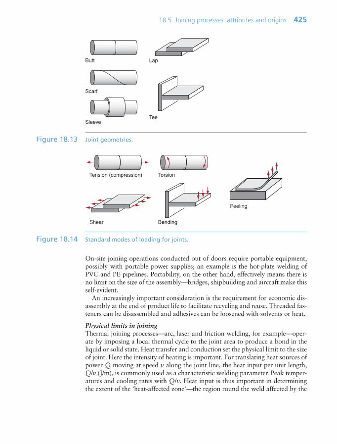
On-site joining operations conducted out of doors require portable equipment,possibly with portable power supplies; an example is the hot-plate welding ofPVC and PE pipelines. Portability, on the other hand, effectively means there isno limit on the size of the assembly—bridges, shipbuilding and aircraft make thisself-evident.
An increasingly important consideration is the requirement for economic dis-assembly at the end of product life to facilitate recycling and reuse. Threaded fas-teners can be disassembled and adhesives can be loosened with solvents or heat.
Physical limits in joiningThermal joining processes—arc, laser and friction welding, for example—oper-ate by imposing a local thermal cycle to the joint area to produce a bond in theliquid or solid state. Heat transfer and conduction set the physical limit to the sizeof joint. Here the intensity of heating is important. For translating heat sources ofpower Q moving at speed v along the joint line, the heat input per unit length,Q/v (J/m), is commonly used as a characteristic welding parameter. Peak temper-atures and cooling rates with Q/v. Heat input is thus important in determiningthe extent of the ‘heat-affected zone’—the region round the weld affected by the
18.5 Joining processes: attributes and origins 425
Butt
Scarf
Sleeve
Lap
Tee
Figure 18.13 Joint geometries.
Shear
Tension (compression) Torsion
Bending
Peeling
Figure 18.14 Standard modes of loading for joints.
Ch18-H8391 1/16/07 6:43 PM Page 425
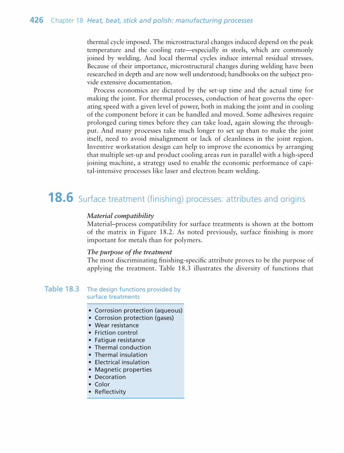
thermal cycle imposed. The microstructural changes induced depend on the peaktemperature and the cooling rate—especially in steels, which are commonlyjoined by welding. And local thermal cycles induce internal residual stresses.Because of their importance, microstructural changes during welding have beenresearched in depth and are now well understood; handbooks on the subject pro-vide extensive documentation.
Process economics are dictated by the set-up time and the actual time formaking the joint. For thermal processes, conduction of heat governs the oper-ating speed with a given level of power, both in making the joint and in coolingof the component before it can be handled and moved. Some adhesives requireprolonged curing times before they can take load, again slowing the through-put. And many processes take much longer to set up than to make the jointitself, need to avoid misalignment or lack of cleanliness in the joint region.Inventive workstation design can help to improve the economics by arrangingthat multiple set-up and product cooling areas run in parallel with a high-speedjoining machine, a strategy used to enable the economic performance of capi-tal-intensive processes like laser and electron beam welding.
18.6 Surface treatment (finishing) processes: attributes and origins
Material compatibilityMaterial–process compatibility for surface treatments is shown at the bottomof the matrix in Figure 18.2. As noted previously, surface finishing is moreimportant for metals than for polymers.
The purpose of the treatmentThe most discriminating finishing-specific attribute proves to be the purpose ofapplying the treatment. Table 18.3 illustrates the diversity of functions that
426 Chapter 18 Heat, beat, stick and polish: manufacturing processes
• Corrosion protection (aqueous)• Corrosion protection (gases)• Wear resistance• Friction control• Fatigue resistance• Thermal conduction• Thermal insulation• Electrical insulation• Magnetic properties• Decoration• Color• Reflectivity
Table 18.3 The design functions provided bysurface treatments
Ch18-H8391 1/16/07 6:43 PM Page 426
surface treatments can provide. Some protect, some enhance performance, stillothers are primarily aesthetic. All surface treatments add cost but the added valuecan be large. Protecting a component surface extends product life and increasesthe interval between maintenance cycles. Coatings on cutting tools enable fastercutting speeds and greater productivity. And surface hardening processes mayenable the substrate alloy to be replaced with a cheaper material—for example,using a plain carbon steel with a hard carburized surface or a coating of hard titanium nitride (TiN), instead of using a more expensive alloy steel.
Secondary compatibilitiesMaterial compatibility and design function are the first considerations in select-ing a finishing process. But there are others. Some surface treatments leave thedimensions, precision and roughness of the surface unchanged. Deposited coatingsobviously change the dimensions a little, but may still leave a perfectly smoothsurface. Others build up a relatively thick layer with a rough surface, requiringrefinishing. Component geometry also influences the choice. ‘Line-of-sight’deposition processes coat only the surface at which they are directed, leavinginaccessible areas uncoated; others, with what is called ‘throwing power’, coatflat, curved and re-entrant surfaces equally well. Many surface-treatment processesrequire heat. These can only be used on materials that can tolerate the rise intemperature. Some paints are applied cold, but many require a bake at up to150°C. Heat treatments like carburizing or nitriding to give a hard surfacelayer require prolonged heating at temperatures up to 800°C. This thermalexposure of the substrate can change the underlying microstructure, not neces-sarily for the better. There are some innovative developments to match the thermaltreatments required in both substrate and surface, achieving two treatments inone go. An example is the paint–bake cycle for heat-treatable aluminum alloyautomotive panels, which cures and hardens the paint while simultaneously agehardening the sheet itself.
Physical limits to surface treatmentsFor thermal processes, the surface heating intensity and absorptivity, and thethermal properties of the substrate, dictate the rise time in temperature. For astationary heat source of given power density, the temperature rises with thesquare root of time
–t . This in turn determines the depth of surface layer that
reaches the temperature at which the desired microstructural change takes place.Since diffusion of matter and heat follow the same mathematical equations, thedepth of treatment in diffusion processes such as carburizing has the samedependence on time. For a spray-coating process delivering a given volumetricflow rate, the coating thickness increases linearly with time.
18.7 Estimating cost for shaping processes
Estimating process costs accurately—at the precision needed for competitivecontract bidding, for example—is a specialized job. It is commonly based on
18.7 Estimating cost for shaping processes 427
Ch18-H8391 1/16/07 6:43 PM Page 427
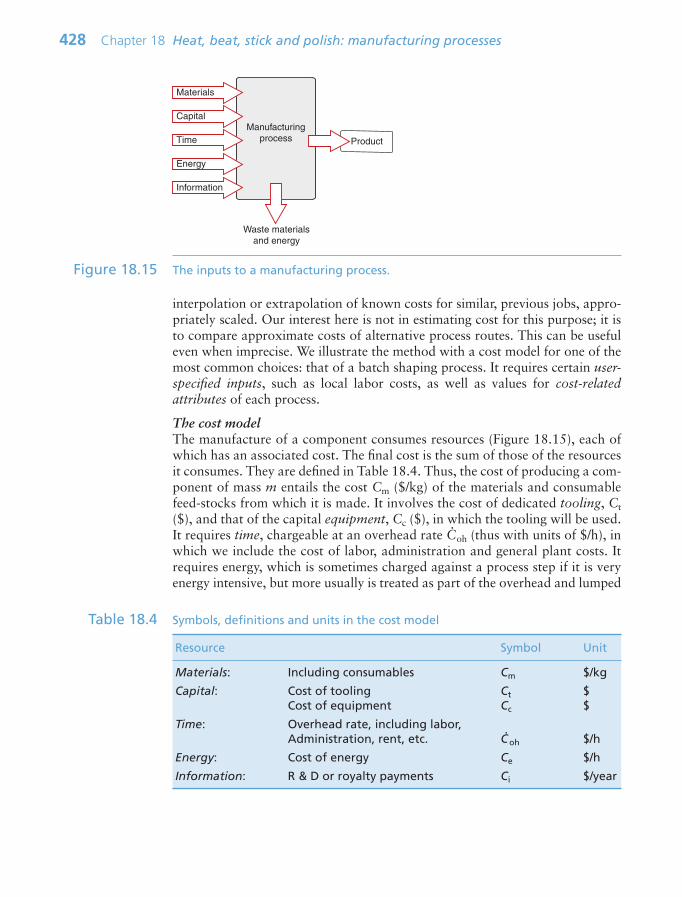
interpolation or extrapolation of known costs for similar, previous jobs, appro-priately scaled. Our interest here is not in estimating cost for this purpose; it isto compare approximate costs of alternative process routes. This can be usefuleven when imprecise. We illustrate the method with a cost model for one of themost common choices: that of a batch shaping process. It requires certain user-specified inputs, such as local labor costs, as well as values for cost-relatedattributes of each process.
The cost modelThe manufacture of a component consumes resources (Figure 18.15), each ofwhich has an associated cost. The final cost is the sum of those of the resourcesit consumes. They are defined in Table 18.4. Thus, the cost of producing a com-ponent of mass m entails the cost Cm ($/kg) of the materials and consumablefeed-stocks from which it is made. It involves the cost of dedicated tooling, Ct($), and that of the capital equipment, Cc ($), in which the tooling will be used.It requires time, chargeable at an overhead rate C
.oh (thus with units of $/h), in
which we include the cost of labor, administration and general plant costs. Itrequires energy, which is sometimes charged against a process step if it is veryenergy intensive, but more usually is treated as part of the overhead and lumped
428 Chapter 18 Heat, beat, stick and polish: manufacturing processes
Product
Materials
Capital
Time
Energy
Information
Manufacturingprocess
Waste materialsand energy
Figure 18.15 The inputs to a manufacturing process.
Resource Symbol Unit
Materials: Including consumables Cm $/kg
Capital: Cost of tooling Ct $Cost of equipment Cc $
Time: Overhead rate, including labor, Administration, rent, etc. C
.oh $/h
Energy: Cost of energy Ce $/h
Information: R & D or royalty payments Ci $/year
Table 18.4 Symbols, definitions and units in the cost model
Ch18-H8391 1/16/07 6:43 PM Page 428

into C.oh, as we shall do here. Finally, there is the cost of information, meaning
that of research and development, royalty or license fees; this, too, we view asa cost per unit time and lump it into the overhead.
Consider now the manufacture of a component (the ‘unit of output’) weigh-ing m kg, and made of a material costing Cm $/kg. The first contribution to theunit cost is that of the material mCm. Processes rarely use exactly the rightamount of material but generate a scrap fraction f, which ends up in runners,risers, machining swarf and rejects. Some is recycled, but the material cost perunit needs to be magnified by the factor 1/(1 f ) to account for the fractionthat is lost. Hence the material contribution per unit is:
(18.2)
The cost Ct of a set of tooling—dies, molds, fixtures and jigs—is what is calleda dedicated cost: one that must be wholly assigned to the production run of thissingle component. It is written off against the numerical size n of the produc-tion run. However, tooling wears out at a rate which depends on the number ofitems processed. We define the tool life nt as the number of units that a set oftooling can make before it has to be replaced. We have to use one tooling seteven if the production run is only one unit. But each time the tooling is replacedthere is a step up in the total cost to be spread over the whole batch. To capturethis with a smooth function, we multiply the cost of a tooling set Ct by(1 n/nt). Thus, the tooling cost per unit takes the form:
(18.3)
The capital cost of equipment, Cc, by contrast, is rarely dedicated. A givenpiece of equipment—a powder press, for example—can be used to make manydifferent components by installing different die-sets or tooling. It is usual toconvert the capital cost of non-dedicated equipment and the cost of borrowingthe capital itself into an overhead by dividing it by a capital write-off time, two,(5 years, say) over which it is to be recovered. The quantity Cc/two is then a costper hour—provided the equipment is used continuously. That is rarely the case,so the term is modified by dividing it by a load factor, L—the fraction of timefor which the equipment is productive. This gives an effective hourly cost of the equipment, like a rental charge, even though it is your own piece of kit. Thecapital contribution to the cost per unit is then this hourly cost divided by theproduction rate/hour n
.at which units are produced:
(18.4)Cn
C
Lt3c
wo
1
⎛
⎝⎜⎜⎜⎜
⎞
⎠⎟⎟⎟⎟⎟
CC
nnn2
t
t
1⎛
⎝⎜⎜⎜⎜
⎞
⎠⎟⎟⎟⎟⎟
CmC
f1m
1
( )
18.7 Estimating cost for shaping processes 429
Ch18-H8391 1/16/07 6:43 PM Page 429

Finally, there is the general background hourly overhead rate C.oh for labor,
energy and so on. This is again converted to a cost per unit by dividing by theproduction rate n
.units per hour:
(18.5)
The total shaping cost per part, Cs, is the sum of these four terms, C1–C4,taking the form:
(18.6)
To emphasize the simple form of this equation, it can be written:
(18.7)
This equation shows that the cost has three essential contributions—a materialcost per unit of production that is independent of batch size and rate, a dedicatedcost per unit of production that varies as the reciprocal of the production volume(1/n), and a gross overhead per unit of production that varies as the reciprocal ofthe production rate (1/n
.). The dedicated cost, the effective hourly rate of capital
write-off and the production rate can all be defined by a representative range foreach process; target batch size n, the overhead rate C
.oh, the load factor L and the
capital write-off time two must be defined by the user.Figure 18.16 uses equation (18.6). It is a plot of cost, Cs, against batch size,
n, comparing the cost of casting a small aluminum component by three alter-native processes: sand casting, die casting and low-pressure casting. At smallbatch sizes the unit cost is dominated by the ‘fixed’ costs of tooling (the secondterm on the right of equation (18.6)). As the batch size n increases, the contri-bution of this to the unit cost falls (provided, of course, that the tooling has alife that is greater than n) until it flattens out at a value that is dominated by the‘variable’ costs of material, labor and other overheads. Competing processesdiffer in tooling cost Ct, equipment cost Cc and production rate n
.. Sand-casting
equipment is cheap but slow. Die-casting equipment costs much more but isalso much faster. Mold costs for low-pressure die casting are greater than forsand casting; those for high pressure die casting are higher still. The combina-tion of all these factors for each process causes the Cs–n curves to cross, asshown in Figure 18.16.
The crossover means that the process that is cheapest depends on the batchsize. This suggests the idea of an economic batch size—a range of batches for
C CC
n
C Cs material
dedicated capital overhe
aad
n
CmC
f
C
nnn n
C
Ltsm t
t
c
wo(1 )1
1⎛
⎝⎜⎜⎜⎜
⎞
⎠⎟⎟⎟⎟⎟
Coh
⎛
⎝⎜⎜⎜⎜
⎞
⎠⎟⎟⎟⎟⎟
CC
n4oh
430 Chapter 18 Heat, beat, stick and polish: manufacturing processes
Ch18-H8391 1/16/07 6:43 PM Page 430
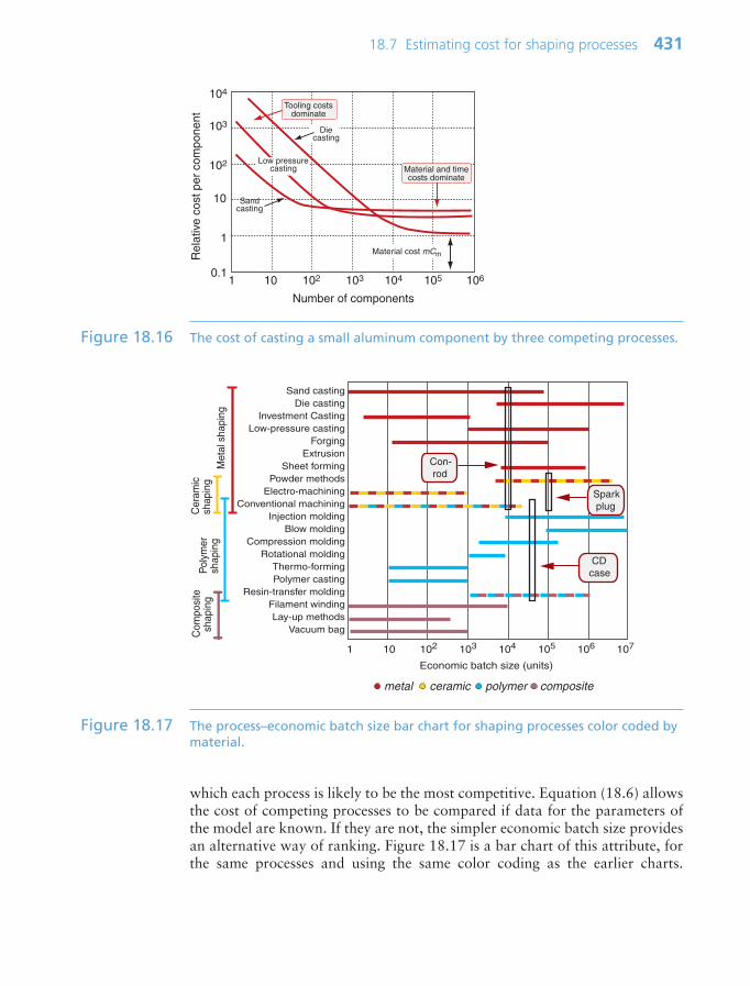
which each process is likely to be the most competitive. Equation (18.6) allowsthe cost of competing processes to be compared if data for the parameters ofthe model are known. If they are not, the simpler economic batch size providesan alternative way of ranking. Figure 18.17 is a bar chart of this attribute, forthe same processes and using the same color coding as the earlier charts.
18.7 Estimating cost for shaping processes 431
Number of components
Rel
ativ
e co
st p
er c
ompo
nent
1 10 102 103 104 105 106
102
104
0.1
1
10
103Die
casting
Sandcasting
Low pressurecasting
Tooling costsdominate
Material cost mCm
Material and timecosts dominate
Figure 18.16 The cost of casting a small aluminum component by three competing processes.
Sand castingDie casting
Investment Casting
ForgingExtrusion
Sheet formingPowder methods
Conventional machiningInjection molding
Blow moldingCompression molding
Rotational molding
Polymer casting
Filament winding
Low-pressure casting
Thermo-forming
Lay-up methodsVacuum bag
Resin-transfer molding
Electro-machining
Met
al s
hapi
ng
Cer
amic
shap
ing
Pol
ymer
shap
ing
Com
posi
te s
hapi
ng
Economic batch size (units)
1 10 102 103 104 105 106 107
Spark plug
CDcase
Con- rod
metal ceramic polymer composite
Figure 18.17 The process–economic batch size bar chart for shaping processes color coded bymaterial.
Ch18-H8391 1/16/07 6:43 PM Page 431

Processes such as investment casting of metals and lay-up methods for compos-ites have low tooling costs but are slow; they are economic when you want tomake a small number of components but not when you want a large one. Thereverse is true of the die casting of metals and the injection molding of poly-mers: they are fast, but the tooling is expensive.
18.8 Computer-aided process selection
Computer-aided selectionAs with the material charts, the process charts of this chapter give an overview,but the number of processes that can be shown on any one of them is limited.Selection using them is practical when there are few constraints, but when thereare many—as there usually are—checking that a given process meets them allis cumbersome, and the cost model cannot be presented in a useful way becauseof the need for user-defined parameters. All these problems are overcome in theCES implementation of the method.
Its database contains records for processes, organized into the families, classesand members shown in Figures 2.5–2.7 of Chapter 2. Each record containsattribute data for a process, with each attribute stored as a range spanning itsusual values, and is linked to the records for the materials it can process. It also contains limited documentation in the form of text, images and references tosources of information about the process. The data are interrogated by thesame search engine that is used for material selection, allowing superimposedstages like those suggested by Figure 18.18. On the left is a stage that limits the
432 Chapter 18 Heat, beat, stick and polish: manufacturing processes
All processes
Process short-list
1
106
Eco
nom
ic b
atch
siz
e
MachiningInjection molding
Die casting
Investment casting
Prototyping
Sand casting
Polymer casting
Selectionbox
Polymers
Elastomers
Ceramics
Glasses
Metals
Hybrids
ThermoplasticsThermosets
Mate
rials
Selectedmaterial class
Prismatic
3-D solid
Section mmMass range kg
Tolerance mm
Shape class
Sheet
etc
Desired attributes
2 3
X
0.5
1 2
FerrousNon-ferrous
Figure 18.18 Schematic of the screening steps in selecting process (here for shaping). Firstspecify classes such as material and shape; then screen on numeric attributes,plotted graphically to the right as bar charts. In the CES software, target designrequirements can also be entered through dialog boxes, shown in the center.
Ch18-H8391 1/16/07 6:43 PM Page 432
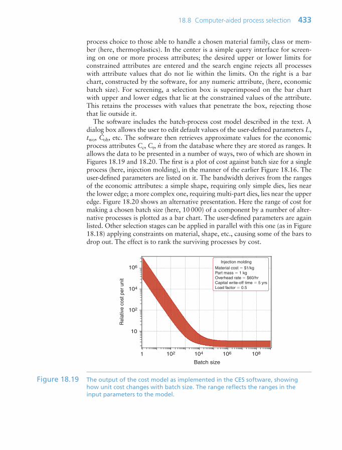
process choice to those able to handle a chosen material family, class or mem-ber (here, thermoplastics). In the center is a simple query interface for screen-ing on one or more process attributes; the desired upper or lower limits forconstrained attributes are entered and the search engine rejects all processeswith attribute values that do not lie within the limits. On the right is a barchart, constructed by the software, for any numeric attribute, (here, economicbatch size). For screening, a selection box is superimposed on the bar chartwith upper and lower edges that lie at the constrained values of the attribute.This retains the processes with values that penetrate the box, rejecting thosethat lie outside it.
The software includes the batch-process cost model described in the text. Adialog box allows the user to edit default values of the user-defined parameters L,two, C
.oh, etc. The software then retrieves approximate values for the economic
process attributes Cc, Ct, n.
from the database where they are stored as ranges. Itallows the data to be presented in a number of ways, two of which are shown inFigures 18.19 and 18.20. The first is a plot of cost against batch size for a singleprocess (here, injection molding), in the manner of the earlier Figure 18.16. Theuser-defined parameters are listed on it. The bandwidth derives from the rangesof the economic attributes: a simple shape, requiring only simple dies, lies nearthe lower edge; a more complex one, requiring multi-part dies, lies near the upperedge. Figure 18.20 shows an alternative presentation. Here the range of cost formaking a chosen batch size (here, 10 000) of a component by a number of alter-native processes is plotted as a bar chart. The user-defined parameters are againlisted. Other selection stages can be applied in parallel with this one (as in Figure18.18) applying constraints on material, shape, etc., causing some of the bars todrop out. The effect is to rank the surviving processes by cost.
18.8 Computer-aided process selection 433
Batch size
Rel
ativ
e co
st p
er u
nit
1 102 104 106 108
10
102
104
106Injection molding
Material cost $1/kgPart mass 1 kgOverhead rate $60/hrCapital write-off time 5 yrsLoad factor 0.5
Figure 18.19 The output of the cost model as implemented in the CES software, showinghow unit cost changes with batch size. The range reflects the ranges in theinput parameters to the model.
Ch18-H8391 1/16/07 6:43 PM Page 433
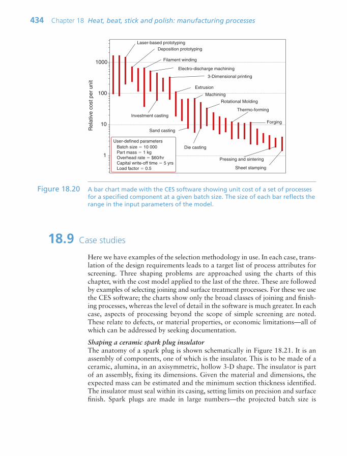
18.9 Case studies
Here we have examples of the selection methodology in use. In each case, trans-lation of the design requirements leads to a target list of process attributes forscreening. Three shaping problems are approached using the charts of thischapter, with the cost model applied to the last of the three. These are followedby examples of selecting joining and surface treatment processes. For these we usethe CES software; the charts show only the broad classes of joining and finish-ing processes, whereas the level of detail in the software is much greater. In eachcase, aspects of processing beyond the scope of simple screening are noted.These relate to defects, or material properties, or economic limitations—all ofwhich can be addressed by seeking documentation.
Shaping a ceramic spark plug insulatorThe anatomy of a spark plug is shown schematically in Figure 18.21. It is anassembly of components, one of which is the insulator. This is to be made of aceramic, alumina, in an axisymmetric, hollow 3-D shape. The insulator is partof an assembly, fixing its dimensions. Given the material and dimensions, theexpected mass can be estimated and the minimum section thickness identified.The insulator must seal within its casing, setting limits on precision and surfacefinish. Spark plugs are made in large numbers—the projected batch size is
434 Chapter 18 Heat, beat, stick and polish: manufacturing processes
Rel
ativ
e co
st p
er u
nit
1
10
100
1000
Laser-based prototypingDeposition prototyping
Extrusion
Sheet stamping
3-Dimensional printing
Machining
Die casting
Rotational Molding
Investment casting
Electro-discharge machining
Filament winding
Sand casting
Pressing and sintering
Forging
Thermo-forming
User-defined parametersBatch size 10 000Part mass 1 kgOverhead rate $60/hrCapital write-off time 5 yrsLoad factor 0.5
Figure 18.20 A bar chart made with the CES software showing unit cost of a set of processesfor a specified component at a given batch size. The size of each bar reflects therange in the input parameters of the model.
Ch18-H8391 1/16/07 6:43 PM Page 434
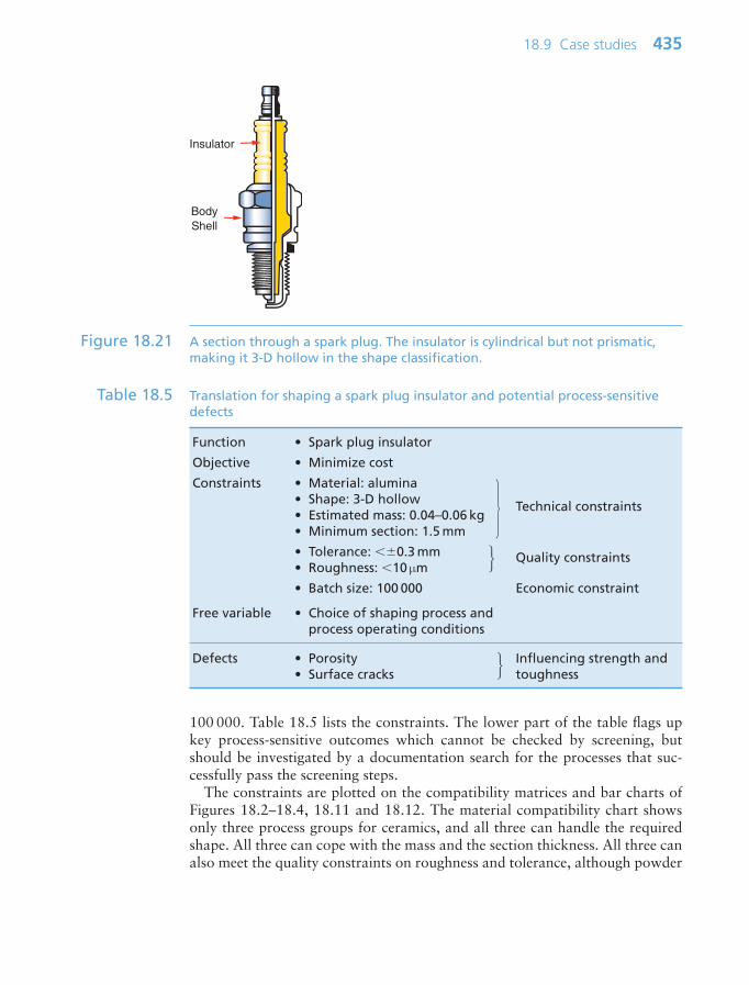
100 000. Table 18.5 lists the constraints. The lower part of the table flags upkey process-sensitive outcomes which cannot be checked by screening, butshould be investigated by a documentation search for the processes that suc-cessfully pass the screening steps.
The constraints are plotted on the compatibility matrices and bar charts ofFigures 18.2–18.4, 18.11 and 18.12. The material compatibility chart showsonly three process groups for ceramics, and all three can handle the requiredshape. All three can cope with the mass and the section thickness. All three canalso meet the quality constraints on roughness and tolerance, although powder
18.9 Case studies 435
BodyShell
Insulator
Figure 18.21 A section through a spark plug. The insulator is cylindrical but not prismatic,making it 3-D hollow in the shape classification.
Function • Spark plug insulator
Objective • Minimize cost
Constraints • Material: alumina• Shape: 3-D hollow• Estimated mass: 0.04–0.06 kg Technical constraints
• Minimum section: 1.5 mm
• Tolerance: 0.3 mm Quality constraints• Roughness: 10 µm
• Batch size: 100 000 Economic constraint
Free variable • Choice of shaping process and process operating conditions
Defects • Porosity Influencing strength and • Surface cracks toughness
Table 18.5 Translation for shaping a spark plug insulator and potential process-sensitivedefects
Ch18-H8391 1/16/07 6:43 PM Page 435
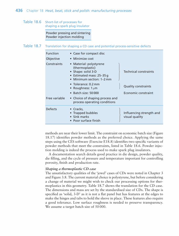
methods are near their lower limit. The constraint on economic batch size (Figure18.17) identifies powder methods as the preferred choice. Applying the samesteps using the CES software (Exercise E18.8) identifies two specific variants ofpowder methods that meet the constraints, listed in Table 18.6. Powder injec-tion molding is indeed the process used to make spark plug insulators.
A documentation search details good practice in die design, powder quality,die filling, and the cycle of pressure and temperature important for controllingporosity, finish and production rate.
Shaping a thermoplastic CD caseThe unsatisfactory qualities of the ‘jewel’ cases of CDs were noted in Chapter 3and Figure 3.8. The current material choice is polystyrene, but before consideringa change of material we might wish to check our processing options for ther-moplastics in this geometry. Table 18.7 shows the translation for the CD case.The dimensions and mass are set by the standardised size of CDs. The shape isspecified as ‘solid, 3-D’ as it is not a flat panel but has features at the edges tomake the hinges and tabs to hold the sleeve in place. These features also requirea good tolerance. Low surface roughness is needed to preserve transparency.We assume a target batch size of 50 000.
436 Chapter 18 Heat, beat, stick and polish: manufacturing processes
Powder pressing and sinteringPowder injection molding
Table 18.6 Short-list of processes forshaping a spark plug insulator
Function • Case for compact disc
Objective • Minimize cost
Constraints • Material: polystyrene (thermoplastic)
• Shape: solid 3-D Technical constraints• Estimated mass: 25–35 g• Minimum section: 1–2 mm
• Tolerance: 0.2 mmQuality constraints• Roughness: 1 µm
• Batch size: 50 000 Economic constraint
Free variable • Choice of shaping process and process operating conditions
Defects • Cracks,• Trapped bubbles Influencing strength and • Sink marks visual quality• Poor surface finish
Table 18.7 Translation for shaping a CD case and potential process-sensitive defects
Ch18-H8391 1/16/07 6:43 PM Page 436

Refer again to the compatibility matrices and bar charts. Screening on thematerial (thermoplastic), shape, mass and minimum section leads to three pos-sible processes: machining, injection molding and compression molding.Compression molding is just beyond its normal mass range. All three processesmeet the targets for tolerance and roughness. The final bar chart shows thatmachining is not economic for the given batch size, but the other two areacceptable. Table 18.8 summarizes the surviving processes.
Good die design to include the protruding ridges and tabs on a CD caserequires expert input. These re-entrant features exclude compression moldingusing uniaxial loading and open dies. Following up the avoidance of defects, adocumentation search is principally a matter of good die design with correctlocation of the runners and risers.
Shaping a steel connecting rodFigure 18.22 shows a schematic connecting rod (‘con-rod’) to be made of amedium carbon steel. The minimum section is around 8 mm, and an estimate ofthe volume gives a mass around 0.35 kg. Dimensional precision is important toensure clearances at both the little and the big end. The con-rod carries cyclicloads with the consequent risk of fatigue crack initiation, so a low surface rough-ness overall is necessary (the bores will be finished by a subsequent machiningoperation). A modest batch size of 10 000 is required. Control of properties
18.9 Case studies 437
Injection moldingCompression molding
Table 18.8 Short-list of processes forshaping a polymer CD case
80.25
14.00.02
18.0 0.02
280.25R 5 µm
Figure 18.22 A steel connecting rod. The precision required for the bores and bore facing ismuch higher than for the rest of the body, requiring subsequent machining.
Ch18-H8391 1/16/07 6:43 PM Page 437

and of defects is dominated by the need to avoid fatigue failure. Table 18.9 summarizes.
These constraints are plotted on the matrices and charts. Screening on materialand shape eliminates low-pressure casting, die casting, extrusion and sheet form-ing, but plenty of options survive. Sand casting is disqualified by the tolerance con-straint. Investment casting, conventional machining, forging and powder methodsremain. All achieve the target roughness, and surface tolerance, though not thatrequired for the bores. However, by following the shaping process with a finishingprocess, the tolerance requirement can be reached. All of the finishing processes atthe bottom of Figure 18.11 give better tolerance and roughness than specified—precision machining is most appropriate for finishing the bores and the faces sur-rounding them. Finally, the economic batch size chart suggests that forging andpowder methods are suitable—machining (from solid) and investment casting arenot economic for a batch size of 10 000. Table 18.10 summarizes.
This case study reveals that there is close competition for the manufacture ofcarbon steel components in the standard mid-range size and shape of a connect-ing rod. Surface finish and accuracy present some problems, but finishing by
438 Chapter 18 Heat, beat, stick and polish: manufacturing processes
Function • Connecting rod (‘con-rod’)
Objective • Minimize cost
Constraints • Material: medium-carbon steel• Shape: 3-D solid• Estimated mass: 0.3–0.4 kg Technical constraints
• Minimum section: 8 mm
• Tolerance: 0.25 mm (surface)• Tolerance: 0.02 mm (bores) Quality constraints• Roughness: 5 µm
• Batch size: 10 000 Economic constraint
Free variable • Choice of shaping process and process operating conditions
Defects • Cracks, surface roughness• Porosity Influencing fatigue • Residual stress resistance
Table 18.9 Translation for shaping a steel connecting rod and potential process-sensitivedefects
Die castingForging machiningPowder methods machining
Table 18.10 Short-list of processes for shaping a steel connecting rod
Ch18-H8391 1/16/07 6:43 PM Page 438
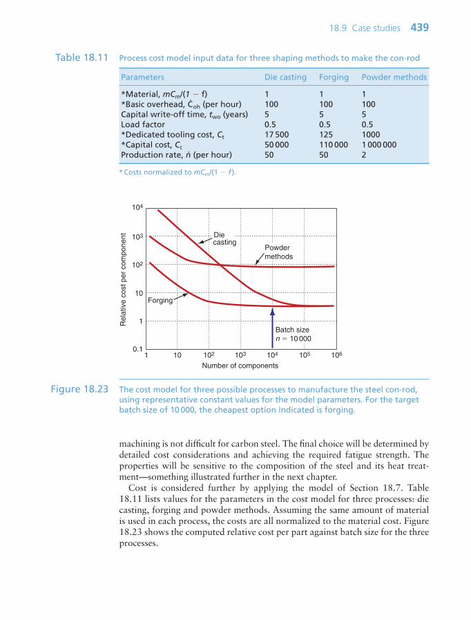
machining is not difficult for carbon steel. The final choice will be determined bydetailed cost considerations and achieving the required fatigue strength. Theproperties will be sensitive to the composition of the steel and its heat treat-ment—something illustrated further in the next chapter.
Cost is considered further by applying the model of Section 18.7. Table18.11 lists values for the parameters in the cost model for three processes: diecasting, forging and powder methods. Assuming the same amount of materialis used in each process, the costs are all normalized to the material cost. Figure18.23 shows the computed relative cost per part against batch size for the threeprocesses.
18.9 Case studies 439
Number of components
Rel
ativ
e co
st p
er c
ompo
nent
1 10 102 103 104 105 106
104
103
102
10
1
0.1
Diecasting
Forging
Powdermethods
Batch sizen 10 000
Figure 18.23 The cost model for three possible processes to manufacture the steel con-rod,using representative constant values for the model parameters. For the targetbatch size of 10 000, the cheapest option indicated is forging.
Parameters Die casting Forging Powder methods
*Material, mCm/(1 f) 1 1 1*Basic overhead, C
.oh (per hour) 100 100 100
Capital write-off time, two (years) 5 5 5Load factor 0.5 0.5 0.5*Dedicated tooling cost, Ct 17 500 125 1000*Capital cost, Cc 50 000 110 000 1 000 000Production rate, n
.(per hour) 50 50 2
Table 18.11 Process cost model input data for three shaping methods to make the con-rod
* Costs normalized to mCm/(1 f ).
Ch18-H8391 1/16/07 6:43 PM Page 439

For the batch size of 10 000 forging comes out the cheapest, followed closelyby die casting. Powder is more expensive, principally because the slower pro-duction rate and high capital cost give a large overhead contribution per part.Since there is a spread of estimated cost (due to uncertainty in the inputs), andforging is likely to be followed by machining, the cost difference between forg-ing and die casting is not significant—both remain on the list for investigationof the achievable properties.
Joining a steel radiatorFigure 18.24 shows a section through a domestic radiator made from corru-gated pressed sheet steel. The task is to choose a joining process for the seamsbetween the sheets. As always, the process must be compatible with the mate-rial (here, low-carbon steel sheet of thickness 1.5 mm). The lap joints carry onlylow loads in service but handling during installation may impose tension andshear. They must conduct heat, be watertight and able to tolerate temperaturesup to 100°C. There is no need for the joints to be disassembled for recycling atthe end of life, since the whole thing is steel. Quality constraints are not severe,but distortion and residual stress will make fit-up of adjacent joints difficult.Low-carbon steels are readily weldable, so it is unlikely that there is a risk ofany welding process causing cracking or embrittlement problems—but this canbe checked by seeking documentation. Table 18.12 summarizes the translation.
To tackle this selection we use the Cambridge Engineering Selector. It storesrecords and attributes for 52 joining processes. Applying the material compat-ibility check first, 32 processes are found to be suitable for joining low-carbonsteel—those eliminated are principally polymer-specific processes. Further screen-ing on joint geometry, mode of loading and section thickness reduces the list to20 processes. The requirement to conduct heat is then the most discriminating—only 10 processes now pass. Water resistance and operating temperature do not
440 Chapter 18 Heat, beat, stick and polish: manufacturing processes
Figure 18.24 A section through a domestic radiator. The three pressed steel sections arejoined by lap joints
Ch18-H8391 1/16/07 6:43 PM Page 440
change the short-list further. The processes passing the screening stage are listedin Table 18.13.
Quality and economic criteria are difficult to apply as screening steps inselecting joining processes. At this point we seek documentation for theprocesses. This reveals that explosive welding requires special facilities and per-mits (hardly a surprise). Electron beam and laser welding require expensiveequipment, so use of a shared facility would be necessary to make them eco-nomic. Resistance spot welding is screened out because it failed the require-ment to be watertight. This is only necessary for the edge seams, so internaljoint lines could be spot welded. This highlights the need for judgement in
18.9 Case studies 441
Function • Domestic radiator
Objective • Minimize cost
Constraints • Material compatibility: low-carbon steel
• Joint geometry: lap joint• Mode of loading: tension,
shear (moderate) Technical constraints• Sheet thickness: 1–2 mm • Joint must conduct heat• Joint must be watertight• Service temperature 100°C• Disassembly not required Environmental constraint
Free variable • Choice of shaping process and process operating conditions
Defects • Residual stress Influencing fit-up and • Imperfect joint service life
Table 18.12 Translation for joining a steel radiator and outcome (potential process-sensitivedefects and properties
BrazingElectron beam weldingExplosive weldingMetal inert gas arc welding (MIG)Tungsten inert gas arc welding (TIG)Laser beam weldingManual metal arc welding (MMA)Oxyacetylene weldingRivetingSoldering
Table 18.13 Short-list of processes for joining a steel radiator
Ch18-H8391 1/16/07 6:43 PM Page 441

applying automated screening steps. Always ask: has an obvious (or existing)solution been eliminated? Why was this? Has something narrowly failed, sothat a low-cost option could be accommodated with modest redesign? Could asecond process step, like sealing the spot-welded joint with a mastic, correct adeficiency? The best way forward is to turn constraints on and off, and adjustnumerical limits, exploring the options that appear.
Surface hardening a ball-bearing raceThe balls of ball bearing races run in grooved tracks (Figure 18.25). As discussedin Chapter 11, the life of a ball race is limited by wear and by fatigue. Both arelimited by using hard materials. Hard materials, however, are not tough, incur-ring the risk that shock loading or mishandling might cause the race to fracture.The solution is to use an alloy steel, which has excellent bulk properties, and toapply a separate surface treatment to increase the hardness where it matters.We therefore seek processes to surface harden alloy steels for wear and fatigueresistance. The precision of both balls and race is critical, so the process mustnot compromise the dimensions or the surface smoothness. Table 18.14 sum-marizes the translation.
The CES system contains records for 44 surface treatment processes. Manyare compatible with alloy steels. More discriminating is the purpose of thetreatment—to impart fatigue and wear resistance—reducing the list to eight.Imposing the requirement for a very smooth surface knocks out those that coator deform the surface because these compromise the finish. The short-list ofprocesses that survive the screening is given in Table 18.15. Adding the furtherconstraint that the curved surface coverage must be very good leaves just thefirst two: carburizing and carbonitriding, and nitriding.
To get further we turn to documentation for these processes. The hardness ofthe surface and the depth of the hardened layer depend on process variables:the time and temperature of the treatment and the composition of the steel.And economics, of course, enters. Ball races are made in enormous batches andwhile their sizes vary, their geometry does not. This is where dedicated equipment,even if very expensive, is viable.
442 Chapter 18 Heat, beat, stick and polish: manufacturing processes
Ball
Outer race
Cage
Hardened track
Inner race
Figure 18.25 A section through a ball bearing race. The surface of the race is to be hardenedto resist wear and fatigue crack initiation.
Ch18-H8391 1/16/07 6:43 PM Page 442

18.10 Summary and conclusions
Selecting a process follows a strategy much like that for materials: translation ofrequirements, screening of the options, ranking of the processes that survivescreening, ending with a search of documentation for the most promising candi-dates. For processes, translation is straightforward—the requirements convertdirectly into the attributes of the process to be used in the screening step. Processattributes capture their technical capabilities and aspects of product quality. Allprocess families require screening for compatibility with material to which theyare to be applied, but after this the attributes and constraints are specific to thefamily. For shaping, component geometry, precision and finish are most discrim-inating. For joining it is joint shape and mode of loading. For surface treatmentsit is the purpose for which the treatment is applied (wear, corrosion, aesthetics,etc.). Ranking is based on cost if this can be modeled, as it can for batch
18.10 Summary and conclusions 443
Function • Ball-bearing race
Objective • Minimize cost
Constraints • Material: alloy steel• Function of treatment: hardening
for fatigue and wear resistanceTechnical constraints• Curved surface coverage: good
• Precision and surface finish not compromised
Free variable • Choice of surface treatment process and process operating conditions
Defects • Cracks Influencing surface • Residual stress toughness and fatigue
resistance
Table 18.14 Translation for surface hardening a ball-bearing race and potential process-sensitive defects
Carburizing and carbonitridingNitridingInduction and flame hardeningLaser surface hardening and meltingVapor metallizing
Table 18.15 Short-list of processes for hardeningan alloy steel ball race
Ch18-H8391 1/16/07 6:43 PM Page 443
processes. Cost models combine characteristic process attributes such as toolingand capital costs and the production rate, with user-specified parameters such asoverhead rates and required batch size. The economic batch size provides acrude alternative to the cost model—a preliminary indication of the batch sizefor which the process is commonly found to be economic.
Translation of the design requirements frequently points to importantaspects of processing that fall beyond a simple screening process. The avoid-ance of defects, achieving the required modification of material properties, anddetermining the process speed (and thus economics), all involve coupling betweenthe process operating conditions, the material composition and design detail.This highlights the importance of the documentation stage in making the finalchoice of processes, and the need to refine the material and process specificationsin parallel. The next chapter explores aspects of process-property interactionsin more depth.
18.11 Further reading
Ashby, M.F. (2005) Materials Selection in Mechanical Design, 3rd edition, Butterworth-Heinemann, Oxford, UK, Chapter 4. ISBN 0-7506-6168-2. (The source of theprocess selection methodology and cost model, with further case studies, giving asummary description of the key processes in each class.)
ASM Handbook Series (1971–2004) Volume 4, Heat Treatment; Volume 5, SurfaceEngineering; Volume 6, Welding, Brazing and Soldering; Volume 7, Powder MetalTechnologies; Volume 14, Forming and Forging; Volume 15, Casting; and Volume 16,Machining; ASM International, Metals Park, OH, USA. (A comprehensive set ofhandbooks on processing, occasionally updated, and now available online atwww.asminternational.org/hbk/index.jsp.)
Bralla, J.G. (1998) Design for Manufacturability Handbook, 2nd edition, McGraw-Hill, New York, USA. ISBN 0-07-007139-X. (Turgid reading, but a rich mine ofinformation about manufacturing processes.)
Campbell, J. (1991) Casting, Butterworth-Heinemann, Oxford, UK. ISBN 0-7506-1696-2. (The fundamental science and technology of casting processes.)
Houldcroft, P. (1990) Which Process?, Abington Publishing, Abington, Cambridge, UK.ISBN 1-85573-008-1. (The title of this useful book is misleading—it deals only witha subset of joining process: the welding of steels. But here it is good, matching theprocess to the design requirements.)
Kalpakjian, S. and Schmid, S.R. (2003) Manufacturing Processes for EngineeringMaterials, 4th edition, Prentice-Hall, Pearson Education, New Jersey, USA. ISBN 0-13-040871-9. (A comprehensive and widely used text on material processing.)
Lascoe, O.D. (1988) Handbook of Fabrication Processes, ASM International, MetalsPark, Columbus, OH, USA. ISBN 0-87170-302-5. (A reference source for fabricationprocesses.)
Swift, K.G. and Booker, J.D. (1997) Process Selection, from Design to Manufacture,Arnold, London, UK. ISBN 0-340-69249-9. (Details of 48 processes in a standardformat, structured to guide process selection.)
444 Chapter 18 Heat, beat, stick and polish: manufacturing processes
Ch18-H8391 1/16/07 6:43 PM Page 444

18.12 Exercises
18.12 Exercises 445
Exercise E18.1 (a) Explain briefly why databases for initial process selection need to be sub-divided into generic process classes, while material selection can be con-ducted on a single database for all materials.
(b) After initial screening of unsuitable processes, further refinement of theprocess selection usually requires detailed information about the materi-als being processed and features of the design. Explain why this is so, giv-ing examples from the domains of shaping, joining and surface treatment.
Exercise E18.2 A manufacturing process is to be selected for an aluminum alloy piston. Itsweight is between 0.8 and 1 kg, and its minimum thickness is 4–6 mm. Thedesign specifies a precision of 0.5 mm and a surface finish in the range 2–5 µm.It is expected that the batch size will be around 1000 pistons. Use the processattribute charts earlier in the chapter to identify a subset of possible manu-facturing routes, taking account of these requirements. Would the selectionchange if the batch size increased to 10 000?
Exercise E18.3 The choice of process for shaping a CD case was discussed in Section 18.5,but what about the CDs themselves? These are made of polycarbonate(another thermoplastic), but the principal difference from the case is preci-sion. Reading a CD involves tracking the reflections of a laser from micro-scopic pits at the interface between two layers in the disc. These pits aretypically 0.5 µm in size and spacing, and 1.5 µm apart; the tolerance must bebetter than 0.1 µm for the disc to work.
First estimate (or measure) the mass and thickness of a CD. Use the charts tofind a short-list of processes that can meet these requirements, and will be com-patible with the material class. Can these processes routinely achieve the toler-ance and finish needed? See if you can find out how they are made in practice.
Ch18-H8391 1/16/07 6:43 PM Page 445
18.13 Exploring design with CES
446 Chapter 18 Heat, beat, stick and polish: manufacturing processes
Exercise E18.4 Use the ‘Browse’ facility in CES to find:(a) The record for the shaping process injection molding, thermoplastics.
What is its economic batch size? What does this term mean?(b) The machining process water-jet cutting (records for machining processes
are contained in the Shaping data table). What are its typical uses?(c) The joining process friction-stir welding. Can it be used to join
dissimilar materials?(d) The surface treatment process laser hardening. What are the three
variants of this process?
Exercise E18.5 Use the ‘Search’ facility in CES to find:(a) Processes used for boat building.(b) Processes to make bottles.(c) Processes to make tail-light assemblies.(d) Processes for decoration.
Exercise E18.6 Use CES Level 3 to explore the selection of casting process for the productslisted. First check compatibility with material and shape, and make reason-able estimates for the product dimensions (to assess mass and section thick-ness). Then include appropriate values for tolerance, roughness, and economicbatch size.(i) Large cast iron water pipes.(ii) 10 000 Zn alloy toy cars (60 mm long).(iii) Small Ni–Co super-alloy (MAR-M432) gas turbine blades (best
possible tolerance and finish).(iv) Large brass ship propeller.
Exercise E18.7 A small nylon fan is to be manufactured for a vacuum cleaner. The designrequirements are summarized in the Table. Use CES Level 3 to identify thepossible processes, making allowance if necessary for including a secondaryfinishing process. Suggest some aspects of the design that may merit investi-gation of supporting information on the selected processes.
Function • Vacuum cleaner fan
Objective • Minimize cost
Constraints • Material: nylon• Shape: 3-D solid• Mass: 0.1–0.2 kg Technical constraints
• Minimum section: 4 mm
• Tolerance: 0.5 mm• Roughness: 1 µm Quality constraints
• Batch size: 10 000 Economic constraint
Free variable • Choice of shaping process
Ch18-H8391 1/16/07 6:43 PM Page 446
18.14 Exploring the science with CES Elements
18.14 Exploring the science with CES Elements 447
Exercise E18.8 The selection of process for a connecting rod was discussed earlier in thechapter. Conduct the selection using CES Level 3, making reasonable esti-mates for any unspecified requirements. Explore the effect of changing to a3 m con-rod for a ship, of approximate cross-section 10 10 cm, in a batchsize of 10.
Exercise E18.9 Process selection for an aluminum piston was investigated in Exercise E18.2.Further investigation of the economics of gravity die casting and ceramicmold casting is suggested. Plot the cost against batch size for these processes,assuming a material cost of $2/kg and a piston mass of 1 kg. The overheadrate is $70/hour, the capital write-off time is 5 years and the load factor is0.5. Which process is cheaper for a batch size of 1000? Assume that as thepiston is simple in shape, it will fall near the bottom of each cost band.
Exercise E18.10 Two examples of selection of secondary processes were discussed in thechapter. The design requirements were summarized for joining processes fora radiator in Table 18.12 and for hardening a steel bearing race in Table18.14. Use CES Level 3 to check the results obtained. For the radiator prob-lem, use the ‘Pass–Fail table’ feature in CES to see if other processes couldbecome options if the design requirements were modified.
Exercise E18.11 Casting processes require that the metal be melted. Vapor methods likevapor metallizing require that the metal be vaporized. Casting requiresenergy: the latent heat of melting is an absolute lower limit (in fact it requiresmore than four times this). Vaporization requires the latent heat of vaporiza-tion, again as an absolute lower limit. Values for both are contained in theElements database. Make a plot of one against the other. Using these lowerlimits find, approximately, how much more energy-intensive vapor methodsare compared with those that simply melt.
Ch18-H8391 1/16/07 6:43 PM Page 447

This page intentionally left blank

Chapter 19Follow the recipe:
processing and properties
Chapter contents
19.1 Introduction and synopsis 45019.2 Microstructure of materials 45019.3 Microstructure evolution in
processing 45419.4 Processing for properties 46219.5 Case studies 46419.6 Making hybrid materials 47219.7 Summary and conclusions 47419.8 Further reading 47519.9 Exercises 47619.10 Exploring design with CES 477
The Khafji rig disaster. (Image courtesy of Thomas Brinsko with Bic Alliance Magazine.)
Ch19-H8391 1/17/07 11:39 AM Page 449
450 Chapter 19 Follow the recipe: processing and properties
19.1 Introduction and synopsis
Some people are better at multi-tasking than others. The good ones should feelat home in manufacturing. Shaping, finishing and assembling components intoproducts to meet the technical, economic and aesthetic expectations of consumerstoday requires the balancing of many priorities. Earlier chapters have introducedintrinsic properties—strength, resistivity and so on—that depend intimately onmicrostructure, and microstructure depends on processing. Microstructure is notaccessible to observation during processing, so controlling it requires the abilityto predict how a given process step will cause it to evolve or change. So manufac-turers have their work cut out to turn materials reliably into good-quality prod-ucts, while making themselves a decent profit. Manufacturing involves morethan making materials into the right shapes and sticking them together; it isalso responsible for producing properties on target.
There is a parallel with cooking. The recipe lists the ingredients and cookinginstructions: how to mix, beat, heat, finish and present the dish. A good cookdraws on experience (and creativity) to create new dishes with pleasing flavor,consistency and appearance; you might think of these as the attributes of thedish. But if the dish is not a success the first thing the cook might do is to cutright through it and examine what went wrong with its microstructure. Suppose,for instance, the dish is a fruit cake, then the distribution of porosity and fruitconstitute aspects of its microstructure.
Microstructure is key to engineering properties too. Some of its componentsare very small—precipitate particles can consist of clusters of a few atoms. Othersare larger—grains range in size from microns to millimeters. Here our goal is toprovide an overview of the main microstructural features and how they evolveduring processing, with the focus on processing for properties. The essence ofthe chapter is captured by the statement:
Composition Processing : Microstructure Properties
Property charts were used in earlier chapters to illustrate examples of propertychanges imparted by composition and processing. Here we draw the discussiontogether and provide further examples from each of the material classes.
19.2 Microstructure of materials
The ability to tune properties is central to materials processing and design, butit brings with it the need for good process control. Failure to follow the ‘recipe’leads, at best, to scrap and lost revenue and, at worst, to engineering failures(cover picture). We start by drawing together all of the microstructural featuresintroduced in the book, by way of an overview.
MetalsFigure 19.1 summarizes the main microstructural features in metals. Starting atthe bottom with atoms, we have crystalline packing (with the exception of the
Ch19-H8391 1/17/07 11:39 AM Page 450
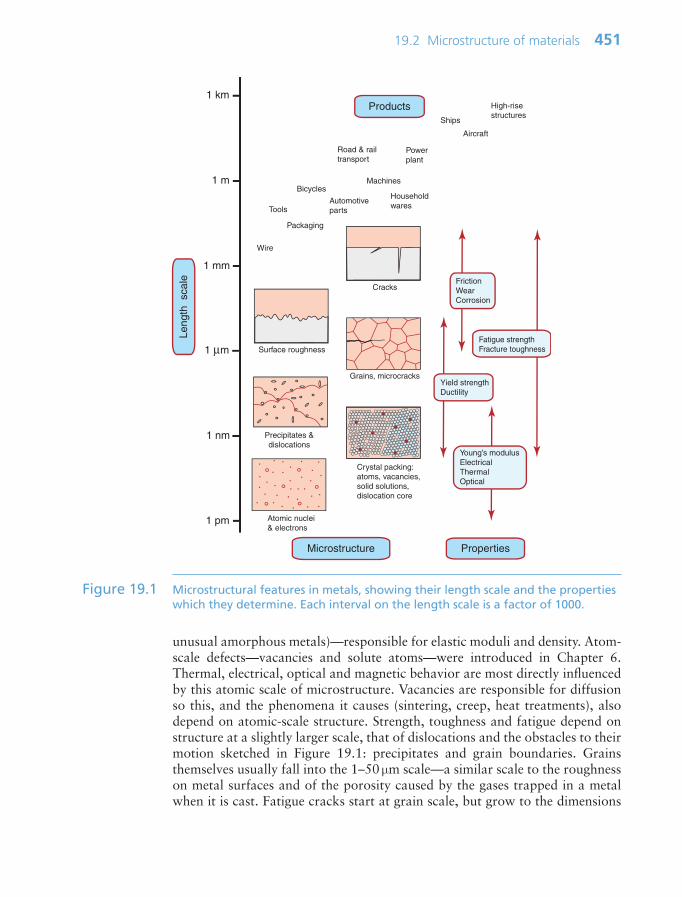
19.2 Microstructure of materials 451
unusual amorphous metals)—responsible for elastic moduli and density. Atom-scale defects—vacancies and solute atoms—were introduced in Chapter 6.Thermal, electrical, optical and magnetic behavior are most directly influencedby this atomic scale of microstructure. Vacancies are responsible for diffusionso this, and the phenomena it causes (sintering, creep, heat treatments), alsodepend on atomic-scale structure. Strength, toughness and fatigue depend onstructure at a slightly larger scale, that of dislocations and the obstacles to theirmotion sketched in Figure 19.1: precipitates and grain boundaries. Grainsthemselves usually fall into the 1–50 µm scale—a similar scale to the roughnesson metal surfaces and of the porosity caused by the gases trapped in a metalwhen it is cast. Fatigue cracks start at grain scale, but grow to the dimensions
1 km
1 m
1 mm
1 µm
1 nm
1 pm
Leng
th s
cale
Surface roughness
Atomic nuclei & electrons
Crystal packing:atoms, vacancies,solid solutions,dislocation core..
..
..
.. . .
........ .
. ..
. .
....
.
.. .
Precipitates &dislocations
Grains, microcracks
Cracks
Properties
Young’s modulusElectricalThermalOptical
Yield strengthDuctility
Fatigue strengthFracture toughness
FrictionWearCorrosion
Products
Microstructure
Wire
Tools
Bicycles
Automotiveparts
Road & railtransport
Ships
Machines
High-risestructures
Householdwares
Packaging
Powerplant
Aircraft
Figure 19.1 Microstructural features in metals, showing their length scale and the propertieswhich they determine. Each interval on the length scale is a factor of 1000.
Ch19-H8391 1/17/07 11:39 AM Page 451

of the component itself at fracture. Metal products themselves span a hugerange: kitchen foil is around 10 µm thick, automotive panels a millimeter or so,ship propellers are several meters in diameter, while bridges and buildings reachthe kilometer scale.
Ceramics and glassesCeramics are crystalline, glasses are amorphous. Figure 19.2 shows both nearthe bottom of our materials length scale. Most of the properties directly reflectthe atomic layout and the intrinsically strong nature of the covalent or ionic
452 Chapter 19 Follow the recipe: processing and properties
1 km
1 m
1 mm
1 µm
1 nm
1 pm
Leng
th s
cale
Atomic nuclei & electrons
Atomic crystal(CERAMICS)
Atomic network(GLASSES)
Grains, microcracks(CERAMICS)
Cracks
Properties
Young’s modulusElectricalThermalOptical
Fracture strengthFracture toughness
FrictionWearCorrosion
Products
Microstructure
. .
. . ..
.
.
..
Microcracks(GLASSES)
Sparkplug
Bridges
Buildings
Bottles
Windows
Electricalinsulators
Cuttingtools
DomesticwhitewareKitchenware
Figure 19.2 Microstructural features in ceramics and glasses, showing their length scale andthe properties which they determine. Each interval on the length scale is a factorof 1000.
Ch19-H8391 1/17/07 11:39 AM Page 452

bonding—from elastic modulus to electrical insulation. The exceptions arestrength and toughness. Cracks dominate failure in ceramics and glasses, sothese are the key features—closely related to grain size (in ceramics) and to thesurface finish.
Polymers and elastomersPolymers and elastomers are inherently molecular rather than atomic. Figure 19.3shows that there is wide diversity at this fine scale: polymer molecules can beamorphous, crystalline, cross-linked or aligned by drawing. Most properties again
19.2 Microstructure of materials 453
1 km
1 m
1 mm
1 µm
1 nm
1 pm
Leng
th s
cale
Atomic nuclei & electrons
Molecular chains,cross-linking
Polymer crystallinity
Crazes, microcracks
Properties
Young’s modulusElectricalThermalOptical
Yield strengthDuctility
Fatigue strengthFracture toughness
Products
Microstructure
C C. .
. .
H
HH
H
Technical textile roofing
Tents
Drinkbottles
Ropes
Packaging
Compact discs
Gardenfurniture
Toys
Automotivetrim
Canoes
Kitchenware
Figure 19.3 Microstructural features in polymers and elastomers, showing their length scaleand the properties which they determine. Each interval on the length scale is afactor of 1000.
Ch19-H8391 1/17/07 11:39 AM Page 453

reflect behavior at this scale, with strength, toughness (and optical properties)bringing in larger features such as crazes and cracks. Polymer foams and fiber-reinforced polymer composites have additional length scales relating to theirarchitecture—for example, pore size and fiber diameter. These and other ‘hybrid’materials are discussed further in Section 19.6.
19.3 Microstructure evolution in processing
The role of shaping processes is to produce the right shape with the rightmicrostructure. Achieving the first requires control of viscous flow or plasticity.Achieving the second means control of the nature and rate of structural evolution.Secondary processing (joining and surface treatment) may cause the structureto evolve further. Examples of microstructural evolution are discussed in latersections, but first some general principles on why and how it happens.
Phases, phase transformations and other structural changeA phase is defined as an arrangement of atoms with a definable structure andcomposition. Steam, water and ice are the vapor, liquid and solid phases of H2O.Engineering alloys such as steel also melt and then vaporize if we heat themenough. More interestingly, they can change phase in the solid state, and it is thisthat gives us precipitation-hardened steels and non-ferrous alloys, made up ofone phase, the precipitate, in a matrix of the other.
Phase transformations are changes of phase during material processing. Theyrequire a driving force and a mechanism. The first is determined by thermody-namics, the second by kinetic theory. The term driving force, somewhat confus-ingly, actually means a change in energy between the starting point (the initialphase or phases) and the end point (the final state). A ball released at the top ofa ramp will roll down it because its potential energy at the bottom is lower thanthat at the top. Here the driving force is the potential energy. Phase changes aredriven by differences in chemical free energy—primarily the internal bond energy(at least in crystalline materials). Solids melt on heating because being a liquidis the state of lowest free energy above the melting point. Chemical compoundscan have lower free energy than solid solutions, so an alloy may decompose intoa mixture of phases (both solutions and compounds) if, in so doing, the totalfree energy is reduced.
Microstructures can therefore only evolve from one state to another if it isenergetically favorable to do so—thermodynamics points the way for change.But changes in microstructure need a mechanism for the atoms to rearrangefrom one structure to another. When a liquid solidifies, there is an interfacebetween the liquid and the growing solid. This is where kinetic theory comesin—atoms transfer from liquid to solid by diffusion at the interface. Virtuallyall solid-state phase changes also involve diffusion to move the atoms around toenable new phases to form. Diffusion occurs at a rate that is strongly dependenton temperature—we calculated it in Chapter 13. The overall rate of structural
454 Chapter 19 Follow the recipe: processing and properties
Ch19-H8391 1/17/07 11:39 AM Page 454

evolution depends on both the magnitude of the driving force (no driving force,no evolution) and the kinetics of the diffusion mechanism by which it takes place.The rates of structural evolution are of great significance in processing. First theygovern the length scale of the important microstructural features—grains, precip-itates and so on—and thus the properties. But they also affect process economics,via the time it takes for the desired structural change to occur.
Solidification and precipitation involve changes in the phases present. Thereare other important types of structure evolution in processing that do notinvolve a phase change, but the principles are the same: there must be a reductionin internal energy, and a kinetic mechanism, for the change to occur. Concentratedsolid solutions have higher free energy than dilute ones, so gradients in concen-tration tend to smooth out, if heated to give the solute atoms enough diffusivemobility. Recovery and recrystallization are mechanisms that change the grainstructure of a crystal. The driving force comes from the stored elastic energy ofthe dislocations in a deformed crystal; the mechanism is diffusive transfer of atomsacross the interface between the deformed and new grain structures.
With that brief introduction, we now illustrate the main changes in structurethat take place in processing, in order to understand what can be manipulatedto achieve the desired properties—or what can go wrong if we don’t followthe recipe.
Solidification: metal castingIn casting, a liquid above its melting point is poured into a mold, where it coolsby conduction. New solid forms by a process of nucleation: tiny crystals formin the melt, either spontaneously or (more usually) on the walls of the containeror on foreign particles in the melt itself (Figure 19.4(a)). As noted above, thenuclei grow by diffusive attachment of atoms at the liquid–solid interface.Solidification is complete when crystals growing in opposing directions impingeon one another, forming grain boundaries—each original nucleus is the originof a grain in the solid (Figure 19.4(b)). The initial grain size of the casting dependson the number of nuclei, since each one grows into a grain. The control of grainsize, important in achieving optimal properties, is achieved by controlling nucle-ation through additions that stimulate it (‘inoculants’) and control of coolingrate. Growing a single crystal is a question of retaining just one nucleus, some-thing that can be done by cooling the liquid slowly from one end so that thefirst nucleus to appear is made to grow along the entire length of the component.The rates of nucleation and growth also depend on the imposed cooling historyand this is governed by heat flow. This is a multi-parameter problem: it dependson the thermal properties of the metal and mold, the contact between the two,the initial liquid temperature, the release of latent heat on solidification, and thesize and shape of the casting. Here is an example of the design–process–materialcoupling discussed in Chapter 18: the geometry of the design combines with thetype of casting process (mold material, metal temperature, etc.) and the choiceof alloy to dictate the cooling rate; and the microstructural response to thatcooling rate (and thus properties) depends on the alloy chemistry.
19.3 Microstructure evolution in processing 455
Ch19-H8391 1/17/07 11:39 AM Page 455
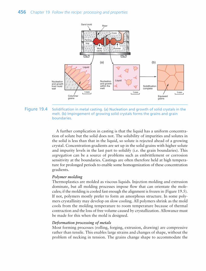
A further complication in casting is that the liquid has a uniform concentra-tion of solute but the solid does not. The solubility of impurities and solutes inthe solid is less than that in the liquid, so solute is rejected ahead of a growingcrystal. Concentration gradients are set up in the solid grains with higher soluteand impurity levels in the last part to solidify (i.e. the grain boundaries). Thissegregation can be a source of problems such as embrittlement or corrosionsensitivity at the boundaries. Castings are often therefore held at high tempera-ture for prolonged periods to enable some homogenization of these concentrationgradients.
Polymer moldingThermoplastics are molded as viscous liquids. Injection molding and extrusiondominate, but all molding processes impose flow that can orientate the mole-cules; if the molding is cooled fast enough the alignment is frozen in (Figure 19.5).If not, polymers mostly prefer to form an amorphous structure. In some poly-mers crystallinity may develop on slow cooling. All polymers shrink as the moldcools from the molding temperature to room temperature because of thermalcontraction and the loss of free volume caused by crystallization. Allowance mustbe made for this when the mold is designed.
Deformation processing of metalsMost forming processes (rolling, forging, extrusion, drawing) are compressiverather than tensile. This enables large strains and changes of shape, without theproblem of necking in tension. The grains change shape to accommodate the
456 Chapter 19 Follow the recipe: processing and properties
1mm 1mm
Liquid
Solidification complete
Equiaxedgrains
Moldcavity
Runner
Sand mold
Parting
line
Core
Riser
Nucleation and growthfrom moldwall
1mm
Liquid
Nucleation and growthwithin themelt
Columnargrains
(a) (b)
Figure 19.4 Solidification in metal casting. (a) Nucleation and growth of solid crystals in themelt. (b) Impingement of growing solid crystals forms the grains and grainboundaries.
Ch19-H8391 1/17/07 11:39 AM Page 456
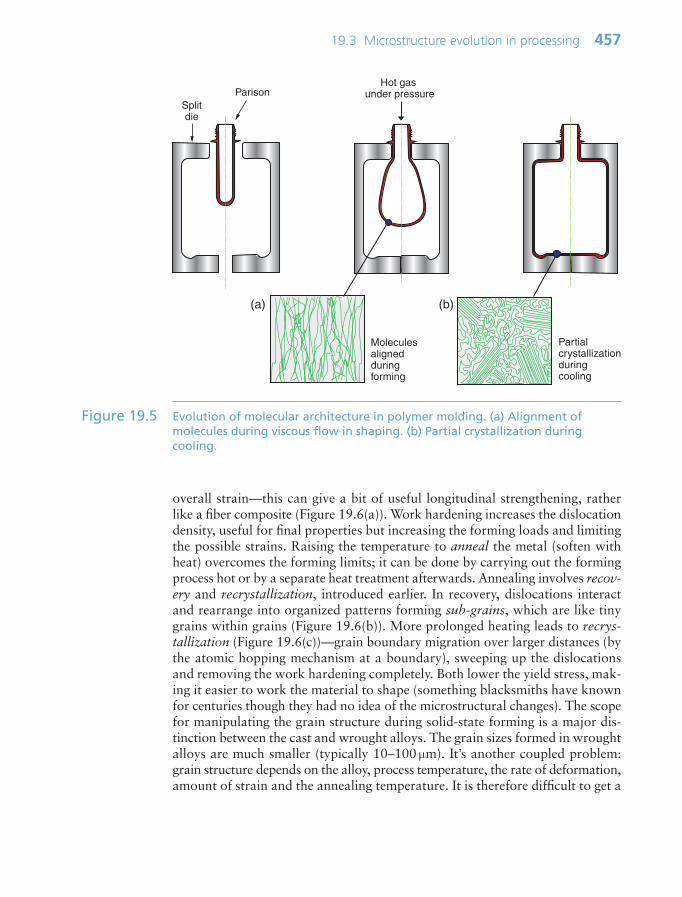
overall strain—this can give a bit of useful longitudinal strengthening, ratherlike a fiber composite (Figure 19.6(a)). Work hardening increases the dislocationdensity, useful for final properties but increasing the forming loads and limitingthe possible strains. Raising the temperature to anneal the metal (soften withheat) overcomes the forming limits; it can be done by carrying out the formingprocess hot or by a separate heat treatment afterwards. Annealing involves recov-ery and recrystallization, introduced earlier. In recovery, dislocations interactand rearrange into organized patterns forming sub-grains, which are like tinygrains within grains (Figure 19.6(b)). More prolonged heating leads to recrys-tallization (Figure 19.6(c))—grain boundary migration over larger distances (bythe atomic hopping mechanism at a boundary), sweeping up the dislocationsand removing the work hardening completely. Both lower the yield stress, mak-ing it easier to work the material to shape (something blacksmiths have knownfor centuries though they had no idea of the microstructural changes). The scopefor manipulating the grain structure during solid-state forming is a major dis-tinction between the cast and wrought alloys. The grain sizes formed in wroughtalloys are much smaller (typically 10–100 µm). It’s another coupled problem:grain structure depends on the alloy, process temperature, the rate of deformation,amount of strain and the annealing temperature. It is therefore difficult to get a
19.3 Microstructure evolution in processing 457
Splitdie
ParisonHot gas
under pressure
Moleculesalignedduringforming
Partialcrystallizationduringcooling
(a) (b)
Figure 19.5 Evolution of molecular architecture in polymer molding. (a) Alignment ofmolecules during viscous flow in shaping. (b) Partial crystallization duringcooling.
Ch19-H8391 1/17/07 11:39 AM Page 457
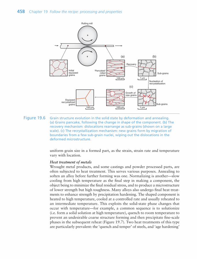
uniform grain size in a formed part, as the strain, strain rate and temperaturevary with location.
Heat treatment of metalsWrought metal products, and some castings and powder processed parts, areoften subjected to heat treatment. This serves various purposes. Annealing tosoften an alloy before further forming was one. Normalizing is another—slowcooling from high temperature as the final step in making a component, theobject being to minimize the final residual stress, and to produce a microstructureof lower strength but high toughness. Many alloys also undergo final heat treat-ments to enhance strength by precipitation hardening. The shaped component isheated to high temperature, cooled at a controlled rate and usually reheated toan intermediate temperature. This exploits the solid-state phase changes thatoccur with temperature—for example, a common sequence is to solutionize(i.e. form a solid solution at high temperature), quench to room temperature toprevent an undesirable coarse structure forming and then precipitate fine-scalephases in the subsequent reheat (Figure 19.7). Two heat treatments of this typeare particularly prevalent: the ‘quench and temper’ of steels, and ‘age hardening’
458 Chapter 19 Follow the recipe: processing and properties
Initialequiaxedgrains
Rolling mill
‘Pancaked’rolledgrains
Sub-grains
Recovery
Sub-grains
Nucleation ofrecrystallization
Growth ofnew grains
100 µm 1 µm
1 µm100 µm100 µm
Equiaxedrecrystallized
grains
(a) (b)
(c)
Figure 19.6 Grain structure evolution in the solid state by deformation and annealing.(a) Grains pancake, following the change in shape of the component. (b) Therecovery mechanism: dislocations rearrange as sub-grains (shown on a largescale). (c) The recrystallization mechanism: new grains form by migration ofboundaries from a few sub-grain nuclei, wiping out the dislocations in thedeformed microstructure.
Ch19-H8391 1/17/07 11:39 AM Page 458
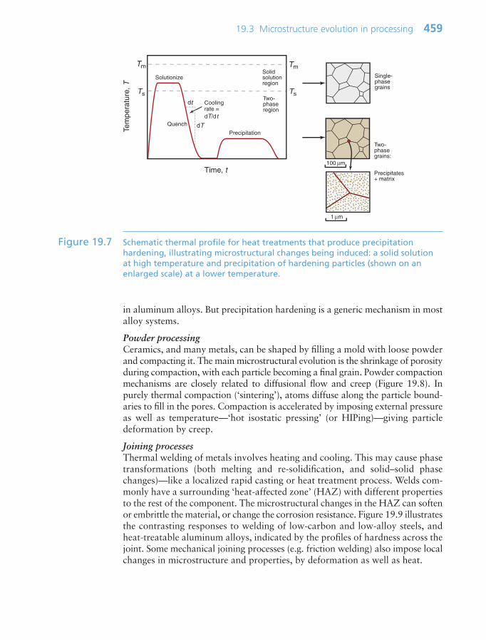
in aluminum alloys. But precipitation hardening is a generic mechanism in mostalloy systems.
Powder processingCeramics, and many metals, can be shaped by filling a mold with loose powderand compacting it. The main microstructural evolution is the shrinkage of porosityduring compaction, with each particle becoming a final grain. Powder compactionmechanisms are closely related to diffusional flow and creep (Figure 19.8). Inpurely thermal compaction (‘sintering’), atoms diffuse along the particle bound-aries to fill in the pores. Compaction is accelerated by imposing external pressureas well as temperature—‘hot isostatic pressing’ (or HIPing)—giving particledeformation by creep.
Joining processesThermal welding of metals involves heating and cooling. This may cause phasetransformations (both melting and re-solidification, and solid–solid phasechanges)—like a localized rapid casting or heat treatment process. Welds com-monly have a surrounding ‘heat-affected zone’ (HAZ) with different propertiesto the rest of the component. The microstructural changes in the HAZ can softenor embrittle the material, or change the corrosion resistance. Figure 19.9 illustratesthe contrasting responses to welding of low-carbon and low-alloy steels, andheat-treatable aluminum alloys, indicated by the profiles of hardness across thejoint. Some mechanical joining processes (e.g. friction welding) also impose localchanges in microstructure and properties, by deformation as well as heat.
19.3 Microstructure evolution in processing 459
Tem
pera
ture
, T
Time, t
TmSolid solutionregion
dt
dT
Cooling rate = dT/d t
Ts
Tm
TsTwo-phaseregion
Solutionize
Precipitation
Quench
Single- phasegrains
Two-phasegrains:
Precipitates+ matrix
.
.
.
.
.. ... .
..
..
.
..
.
.
..
.
..
.
.
.
.
.
.
.
. .. .
. .. ..
.
.
.
..
. ..
...
100 µm. .
.
..
...
.
.
. ..
.. ...
.. .
.
..
... .. . .... .
..
.. .
.
..
... .. . .... .
..
.. .
.
..
... .. . ....
..
.
.. .
.
. .
. .
.
. ... .
..
.
.
. . ... .... . . ... .
.
..
. .. .. .
.
.
..
...
...
.
. . .
..
. ...
.
.. ...
.
.
..
... .. .
.
...
.
.
.
..
.. .
.
..
.
.
..
. ..
.. ...
.
.
.
..
... .. . ..
1 µm
Figure 19.7 Schematic thermal profile for heat treatments that produce precipitationhardening, illustrating microstructural changes being induced: a solid solutionat high temperature and precipitation of hardening particles (shown on anenlarged scale) at a lower temperature.
Ch19-H8391 1/17/07 11:39 AM Page 459

Welding metallurgy is a big field of study—welds are often the ‘Achilles heel’in design, being the critical locations that determine failure and allowable stresses.This may be in part because the material properties are damaged in some wayat the joint (as in this example), but it may also be due to other side-effects ofthe process (residual stresses, or stress concentrations, or crevices, potentiallycausing fatigue and corrosion problems). Adhesive technologies are not troublefree—they still concentrate stress and contain defects, requiring good designand process control—but they have the advantage that they don’t impose heator deformation on the components being joined, leaving the microstructureand properties intact.
Surface engineeringSurface treatments exploit many different mechanisms and processes to changethe surface microstructure and properties. Some simply add a new coating mate-rial, with its own microstructure and properties, leaving the substrate unchanged—the only problem is then making sure they stick. Others induce near-surface phasetransformations by local heating and cooling. Figure 19.10 shows an example—laser hardening of steels, in which the final phase is much harder than the initialstate. Direct diffusion of atoms into the surface is also feasible—but only forinterstitial solute atoms at high temperature for diffusion to occur over a distance
460 Chapter 19 Follow the recipe: processing and properties
Loose- packedpowder
Residualporosity
Diffusion
Sinter in furnaceFill die
Powder
Hot press
‘Green form’
Pore
Grainboundary
20 µm
1 µm
Figure 19.8 Mechanism of powder compaction in hot pressing and sintering.
Ch19-H8391 1/17/07 11:39 AM Page 460

19.3 Microstructure evolution in processing 461
Heat-affectedzone
Weldmetal
Har
dnes
s
Distance
Weld metalHAZ HAZ
Al alloy
Har
dnes
s
Distance
Weld metalHAZ HAZ
Steels
Low-carbonsteel
Alloysteel
Tem
pera
ture
, T
Time, t
Tm
Weld metal
Heat-affectedzone
dt
dT
Cooling rate = dT/dt
Speed, v Weldmetal
Heat-affectedzone
Arc
Electrode
Speed, v
Laserpower, q
Hardenedtrack
Figure 19.9 A weld cross-section with corresponding thermal histories in the weld metal andheat-affected zone. Below are typical hardness profiles induced across welds inheat-treatable aluminum alloys, low-carbon steel and low-alloy steel.
Figure 19.10 Laser hardening: a surface treatment process that modifies microstructure. Thetraversing laser beam induces a rapid thermal cycle, causing phase changes onboth heating and cooling. The track below the path of the laser has a differentfinal microstructure of high hardness.
Ch19-H8391 1/17/07 11:39 AM Page 461
462 Chapter 19 Follow the recipe: processing and properties
of any significance. Chapter 13 revealed that, even near the melting point, thereis a physical limit to diffusion distances (Dt
—–) of around 0.2 mm for a 1-hour
hold, which is sufficient for surface treatments—and for bulk processing on avery small scale (as in semiconductor devices). This mechanism is used to increasethe carbon content (and thus hardness) of steels—the surface treatment knownas carburizing.
19.4 Processing for properties
There is a mantra a few pages back: Composition Processing :Microstructure Properties. Here is an example to flag up general issuesabout this interaction.
Aluminum bike framesThe material chosen for the bike frame, for its good stiffness and fatigue resist-ance at low weight (Chapters 5 and 10), is a heat-treatable aluminum alloy.Figure 19.11 illustrates the main steps in the process history. It makes a numberof points.
Point 1: the chemistry of the chosen alloy is adjusted at the outset of process-ing, in the liquid state, and cannot be changed after casting. Metallic elementsdissolve freely in one another in the liquid state, but it is very difficult to addthem in the solid state; diffusion is much too slow.
Point 2: materials processing involves more than one step. Metal casting,powder processes and polymer molding are near-net-shape processes—the rawmaterial is turned into the shape of the component in a single step, leaving onlyfinishing operations (including heat treatment), so the number of steps is few. Bycontrast, wrought products (those that undergo some deformation processing)involve a longer chain of processes. The initial casting of wrought alloys is mosteconomic on a large scale, so standard compositions are cast into large ingotsas in Figure 19.11(a), which are transported to different factories for processinginto different products. For the bike frame, the ingot is sliced into billets andextruded into tube. The figure shows, in (b), a temperature history for the mate-rial as it is shaped directly from a solid circular billet, around 200 mm in diam-eter, to a hollow tube, 30 mm in diameter and 3 mm thick. The extrusion is donehot to reduce the strength and increase the ductility. This enables the materialto undergo the large plastic strains, allowing fast throughput at relatively lowextrusion force. The quality of surface finish is determined at this stage.
Point 3: design focuses on the properties of the finished product, but some ofthese same properties (strength, ductility, etc.) are critical during processing. Thedesign and the processing characteristics can be in conflict—strong alloys aremore difficult to process and are thus more expensive. So in choosing materialsfor a component it is important to examine their suitability for processing as wellas for performance in service. Returning to the extrusion step of the bicycleframe, we note that extrusion produces the required shape and it also enhances
Ch19-H8391 1/17/07 11:39 AM Page 462

Time, t
10 m
Ingot casting
20 cm
Time, t
100 m
TmExtrusion
30 mm
Time, t
Age hardening
Tem
pera
ture
, T
Time, t
Welding
Solidification
Preheat
Extrude Air/watercooling
Ageing
5 m
30 mm
Weld metal
2–3 hours
Heat-affectedzone
Cast ingot
Extruded tube,rapidly cooled
Stock tube, cut tolength & aged
Weldedbike frame
Tm
T m
Tm
Tem
pera
ture
, TTe
mpe
ratu
re,
TTe
mpe
ratu
re,
T
(a)
(b)
(c)
(d)
Figure 19.11 A schematic process history for the manufacture of a bike frame in heat-treatablealuminum alloy. (a) Casting of large ingot, cut into billets for extrusion. (b) Hotextrusion into tube, incorporating the solution heat treatment and quench.(c) Sections cut to length and age hardened. (d) Assembly into the frame by arcwelding.
Ch19-H8391 1/17/07 11:39 AM Page 463

the microstructure. The hot deformation refines the as-cast grain structure andhelps homogenize the alloy. Forced cooling of the tube as it emerges from theextrusion press quenches it, trapping solute in solution, thus obviating the needfor a subsequent solution heat treatment prior to ageing. The tube is then cutto length and aged as in Figure 19.11(c), giving it its final strength. In a non-heat-treatable aluminum alloy, strength comes from solid solution and workhardening, not precipitation, so the extrusion is then done cold to maximize thework hardening, with no further heat treatment. Deformation and thermal his-tories are critical for controlling shape and final properties simultaneously, butdepend in the detail on the particular alloy variant being processed.
Finally, the frame is assembled by arc welding. In the heat-affected zone theprecipitates carefully produced by age hardening disappear back into solution. Asthe whole age-hardening cycle is difficult to repeat on the completed frame, theheat-affected zone round the weld ends up with different, inferior properties tothe rest of the frame (Figure 19.9). Hence the last point in this short journeythrough a typical metal-processing operation is a reminder: watch out for joiningsteps (especially welding) that undo the good done by earlier process steps.
With this background, we now examine how diverse combinations of chem-istry and processing are used to manipulate properties, in all material classes.The emphasis is on the interaction between processing and the ‘ideal’ propertiesstored in a property database, which can be achieved if all goes to plan. But thebicycle frame case study shows that we need to keep our eyes open in this game,and to be aware of why we often need to compromise between design objectivesand manufacturing realities. The importance of the ‘Seek Documentation’ stagein material and process selection should not be underestimated!
19.5 Case studies
Metals—overviewIt was clear in Chapter 18 that a favorable characteristic of metals is the diver-sity of manufacturing processes available to make and assemble components ofcomplex shape. And the earlier sections have shown how, while shaping andjoining components, the underlying microstructure is being manipulated togenerate the properties needed. This includes both properties during processing(for example, ductility for deep drawing a beer can) and the properties neededin service (for example, strength and toughness for automotive alloys). Processingand service demands can often be in conflict, but there are cunning ways roundthis—e.g. shape it hot (and thus soft) and then heat treat it later (to raise thestrength).
Steels (and other ferrous alloys) are the dominant engineering alloys, butsimilar principles apply to all the alloy systems, such as those based on Al, Cu,Ti, Ni, Zn, Mg and so on. Most alloy systems offer both cast and wrought vari-ants, and many are also processed as powder. Usually either cast or wrought alloysdominate an alloy class. This reflects subtle differences in the ease of deformation
464 Chapter 19 Follow the recipe: processing and properties
Ch19-H8391 1/17/07 11:39 AM Page 464

of the underlying crystal structures in different elements. For example, Zn, Mgand Ti have the ‘hexagonal close-packed (HCP)’ crystal structure (see Chapter 4).This is inherently less ductile than the FCC or BCC crystal structures found inAl, Fe and Cu—so Zn, Mg and Ti are mostly cast, with only limited deformationprocessing being conducted, and usually then done hot (when the ductility isbetter). Ductile Al, Fe and Cu are mostly wrought, but all come as casting alloystoo. Casting and wrought alloys in a given metal system tend to have quite dif-ferent compositions. Good castability requires much higher levels of alloyingadditions than the relatively dilute wrought alloys (to lower the melting point).Casting leads to coarser microstructures and poorer strength and toughness thanin wrought alloys (as illustrated for aluminum alloys in Chapter 8).
To illustrate the details of metals processing and property manipulation further,we now draw on examples from the dominant class: the ferrous alloys.
Ferrous alloysFor structural and mechanical applications, steels and other alloys based on irondominate. They are intrinsically stiff, strong and tough, and mostly low cost.High density is a drawback for transport applications, allowing competitionfrom light alloys, wood and composites. Figure 19.12 illustrates the diversity ofapplications for ferrous alloys. These reflect the many classes of alloy—differentchemistries combined with different process histories. Examining each in turnhighlights the key material property, composition and processing factors at work.
19.5 Case studies 465
(a) (b)
(c) (d)
Figure 19.12 A selection of products made from alloys based on iron. (a) Cast iron: brakedisk. (b) Low-carbon steel: I-beam. (c) Low-alloy steel: connecting rod. (d) Stainless steel: cutlery.
Ch19-H8391 1/17/07 11:39 AM Page 465

Cast iron brake disk. Brake disks (Figure 19.12(a)) use sliding friction on thebrake pads to decelerate a moving vehicle, generating a lot of heat in the process(Chapter 11). The key material properties are therefore hardness (strength) forwear resistance, good toughness and a high maximum service temperature. Lowweight would be nice for a rotating part in a vehicle, but this is secondary. Allferrous alloys fit the bill—so why cast iron? Because casting is the cheapest wayto make the moderately complicated shape of the disk, and the as-cast microstruc-ture does not usually require further heat treatment to provide the hardnessrequired. Cast irons typically contain 2–4% carbon (by weight) giving a lot ofiron carbide—a hard compound giving excellent precipitation hardening. Castiron may also contain free graphite, giving good machinability, the ability to bemachined quickly with minimal or no lubricant—another important ‘propertyduring processing’.
As described in Section 19.3, the grain structure is formed during the shapingprocess and cannot be modified later. The key features to control are the size ofthe grains themselves (e.g. by using inoculants) and the distribution of impurities.Rather than trying to remove impurities from the melt, which is expensive, it isusually possible to render them harmless by giving them something else to reactwith, to form a solid compound distributed throughout the casting. Manganeseis added to ferrous alloys to clean up sulfur, for instance. Tweaking the chemistryof castings to improve their properties has been a bit of a black art for centuries.Nowadays it is possible to use sophisticated software tools to model everythingfrom the choice of composition to the way to pour the metal into the mold inorder to minimize porosity and residual stress.
Plain carbon steel: I-beams, cars and cans. If we had to single out one universallydominant material, we might well choose mild steel—iron containing 0.1–0.2%carbon. Almost all structural sections (Figure 19.12(b)), automotive alloys andsteel packaging (beer and food cans) are made of mild steel (or a variant enhancedwith a few other alloying additions). All of these applications are wrought—thealloy is deformed extensively to shape. The excellent ductility of plain carbonsteel enables this, while the deformation process exploits their work hardeningto give the required product strength. Ductility, toughness and decent strengthare vital in a structural material—we would rather a bridge sagged a little ratherthan broke in two, and in a car crash our lives depend on the energy absorptionof the front of the vehicle.
It was noted earlier that annealing is commonly used to control the grain struc-ture in wrought alloys, including low-carbon steels. An important side-effect ofdeformation followed by annealing is the concept of crystal texture. The crystalplanes in a casting are random—each nucleus forming in isolation within a melt.Not only does deformation ‘pancake’ the grains, it tends to align the crystallo-graphic planes with respect to the axes of the deformation. Perhaps unexpect-edly, recrystallization doesn’t restore randomness—there remains a statisticaldistribution of orientations. This doesn’t sound very important, but it is significantin working with sheet metal, since textured metals have yield properties which
466 Chapter 19 Follow the recipe: processing and properties
Ch19-H8391 1/17/07 11:39 AM Page 466

are anisotropic (i.e. different in different directions). This can be a problem ifyou want to make something smooth and circular out of a sheet, like a bever-age container.
Alloy steels and heat treatment: cranks, tools and gears. The moving and con-tacting parts of machinery (Figure 19.12(c)) are subjected to very demandingconditions—high bulk stresses to transmit loads in bending and torsion (as in acrank or a drive shaft), high contact stresses where they slide or roll over oneanother (as in gears), and often reciprocating loads promoting fatigue failure(as in connecting rods). Strength with good toughness is everything. Plain carbonsteels extend up to 0.8% carbon—this introduces more iron carbide into themicrostructure, giving greater precipitation hardening. They do a reasonable job,but the density of iron is a problem. Make the steel stronger, and use less of it,and we can save weight. This is particularly true for fast-moving parts in engines,since the support structure can also be made lighter if the inertial loading isreduced (so-called ‘secondary weight savings’). The trick is yet more alloying,and more processing.
A bewildering list of additions to carbon steel can be used to improve thestrength—Mn, Ni, Cr, V, Mo and W are just the most important! Some contributedirectly to the strength, giving a solid solution contribution (e.g. high-alloy toolsteels, with up to 20% tungsten). More subtle though is the way quite modestadditions (5% in low-alloy steels) affect the alloy’s response to heat treatment.The key process is ‘quench and temper’ (Figure 19.7). The steel is heated to atemperature at which the carbon and the alloy additions dissolve (850–1000°C)and then quenched rapidly to room temperature, usually in oil or water.Tempering is reheating of the steel to an intermediate temperature to precipi-tate a fine, uniform dispersion of iron carbide in iron in every single grain. Thequench is critical—slow cooling produces a softer mixture of grains, somebeing pure iron and some containing a coarse dispersion of iron carbide. A bitof additional precipitation strength comes from the formation of alloy carbides,but this is not the main reason for alloying. Plain carbon steels can also bequenched and tempered. The problem is the severity of the quench needed toavoid the formation of the much less effective microstructure associated withslow cooling. Alloying effectively shuts this down, enabling slower quench ratesto achieve the target microstructure. In consequence, bigger components can beheat treated this way—the cooling rate at the center being limited by heat conduc-tion through the steel. The technical term for this is enhancing hardenability—it isanother example of how material, process and design detail can interact inmeeting the objectives of a design.
In passing, it is worthy of note that the intermediate microstructure (knownas ‘martensite’) formed on quenching a hardenable steel is very hard, but alsovery brittle—like a ceramic. It is therefore useless as a bulk microstructure—tempering is essential to restore useful toughness. However, some surface treat-ments can produce a thin layer of martensite on a component—excellent for wearresistance on gears, bearings and so on. This is how laser hardening works
19.5 Case studies 467
Ch19-H8391 1/17/07 11:39 AM Page 467

(Figure 19.10). In other respects, martensite is a bit of a hazard. It can causecracking problems on quenching, due to stresses induced by differential thermalcontraction (Chapter 12). And even worse, welding causes a thermal cycle similarto the first stage of heat treatment, so higher carbon and alloy steels are suscep-tible to inadvertent embrittlement if the cooling rate is too quick (Figure 19.9).Oil rigs and bridges have collapsed without warning as a result of this behavior.
Stainless steel: cutlery. The city of Sheffield in England made its name on stainlesssteel cutlery (Figure 19.12(d)), and today manufactures more steel (of all types)than ever before. The addition of substantial amounts of chromium (up to 20%by weight) imparts excellent corrosion resistance to iron, avoiding one of itsmore obvious failings: rust. It works because the chromium reacts more stronglywith the surrounding oxygen, protecting the iron from attack (Chapter 17).Nickel is also usually added for other reasons—one being the preservation ofthe material’s toughness at the very low cryogenic temperatures needed for thestainless steel pressure vessels used to store liquefied gases. Another is that bothchromium and nickel provide solid solution hardening—this and work hardening(during rolling and forging) being the usual routes to strength in stainless steels,rather than heat treatment for precipitation strength.
Summary. In all of these applications, strength and toughness dominate theproperty profile. The manipulation of these properties was illustrated in Chapter 8on a property chart for the main structural light alloys (aluminum). How dothese varied ferrous alloys map out on this chart? Figure 19.13 shows a smallselection of steels of the four types discussed above. This paints a remarkablepicture. Starting with soft, tough pure iron (top left), we can manipulate it toproduce more or less any combination of strength and toughness we like—increasing the strength by more than a factor of 20. Every final material (withthe exception of as-quenched martensite) is comfortably above the typical fracturetoughness threshold (15 MPa.m1/2) for structural or mechanical application.The normalized condition is standard for structural use. The chart shows howthe quench-and-temper treatment enhances the strength without damaging thetoughness. This figure explains why steels are so important—no other materialis so versatile, with literally hundreds of different steels and ferrous alloys avail-able commercially.
Ceramics and glassesBrittle materials have a problem. No matter what other advantages they have,they are susceptible to fracture, which may be traced back in many cases to theinherent defects built in during processing. Ceramic and glass processing formechanical application are therefore about the control of defects. The micro-cracks in ceramics largely reflect the size of powders used in the first place, butgood-quality processing is then needed to avoid porosity. This is surprisinglydifficult to achieve, even in simple shapes. Loose powders contract by a factorof 2 or more when they are pressed and sintered together. Achieving uniformcontraction of this magnitude is not easy, since different regions of the product
468 Chapter 19 Follow the recipe: processing and properties
Ch19-H8391 1/17/07 11:39 AM Page 468

densify first and then constrain the further compaction of the remainder. Glassesare easier to handle as they are melt processed. None the less, great care is takenover achieving a smooth finish—plate glass is mostly produced by flotation on a bath of molten tin. Ceramics and glasses are also very susceptible to thermalstresses during cooling. Being processed at high temperature, but inherently stiffand strong, stresses are not easily relieved by creep during cooling. In one instance,however, thermal stresses are exploited to good effect. Glass can be made morefracture resistant by deliberately generating a residual stress profile through-thickness by cooling the surfaces. This leads to beneficial compression at thesurfaces and tension within—the surface being the likely location of the scratchesand microcracks which cause fracture under tensile load.
Ceramic compositions tend to be largely discrete—each being a specific com-pound (alumina, silicon carbide, etc.). Some composite mixtures are processedtogether, such as tungsten carbide and cobalt, to make a hard, tough material fordies and cutting tools. In contrast, glass compositions can be tuned continuouslyover a wide range to achieve particular combinations of color and other opticalproperties (e.g. the graded compositions used in optical fibers). The adaptablespread of optical properties was evident in the property charts of Chapter 15. Thisis largely a matter of tweaking the chemistry rather than the process. More recentdevelopments with glass processing are associated with coating technology—forscratch and chip resistance (in windscreens), or for self-cleaning and high reflectivityin high-rise buildings.
19.5 Case studies 469
10
100
300
100 1000 3000
Yield strength, σy (MPa)
Frac
ture
toug
hnes
s, K
Ic (
MP
a.m
1/2 )
300
30
Cast irons
Pure iron
Plain C steels,normalized
Alloy steels,quenched & tempered
Plain C steels,quenched &tempered
Stainlesssteel
Tool steel
Alloy & C steels,as-quenched(martensite)
KIc< 5
HRS, 07
Figure 19.13 Fracture toughness—yield strength property chart for ferrous alloys. Compositionand heat treatment enable a wide range of combinations of these properties.
Ch19-H8391 1/17/07 11:39 AM Page 469
Polymers and elastomersPolymers are versatile materials in many respects—easy to mold into complexshapes at low cost, easy to join together by snap fitting and easy to color. Bulkpolymers provide a spread of Young’s modulus, strength and toughness—allrelatively low. Polymer chemistry, and the use of additives and fillers, give enor-mous freedom to adapt the bulk properties, though the ability to make largechanges in strength is more limited than for metals. In contrast, polymers dooffer scope for changing elastic properties, which metals do not.
Chapter 4 introduced the structure of polymers, and how chemistry is usedto produce the thousands of variants available today. Long-chain molecules areproduced by polymerization of a basic monomer unit of carbon, bonded withhydrogen, chlorine, oxygen and so on. Each monomer has a discrete chemistry—C2H4 makes polyethylene, for example. Unlike metal (and non-metal) atoms,monomers do not readily combine with one another. Only selected combinationswill polymerize together, to make copolymers (with two monomers), terpolymers(with three) and so on. For example, ABS is a terpolymer, combining monomersof acrylonitrile, butadiene and styrene (hence the name). Blending polymers extendthe range further, giving a mixture of more than one type of chain molecule—forexample, ABS–PVC. And the molecular architecture itself can be manipulated.As described in Chapter 4, thermosets and elastomers are cross-linked, and somethermoplastics will partially crystallize. Furthermore, bulk polymers usuallycontain additives and fillers, for all sorts of reasons—for example, glass or ceramicparticles or fibers (for stiffness, strength or color), flame retardants, plasticizersor UV protection.
Most of this has only a modest impact on processing of polymers—mostprocesses work with most polymers. Additives change the viscosity, so the easeof injection molding will be influenced by the volume fraction of filler. Fusionwelding only works for non-cross-linked thermoplastics, which can be re-melted.And, as noted earlier, crystallization is sensitive to temperature history—therate of cooling of a molding will have some influence on the final stiffness andstrength, as well as the dimensional precision. Processing can, however, play asignificant role in determining the final molecular arrangement, and thus prop-erties, if the molecules are aligned mechanically during the shaping process.Figure 19.5 showed the blow molding of a drinks bottle, from a pre-form closedtube called a parison. The stretching process of inflating the parison aligns themolecules in the bottle wall, enhancing stiffness and strength.
The most dramatic impact of processing on polymer properties is in makingfibers. These are drawn from the melt, or for even better results, cold drawn.Now the molecular alignment is much more marked, so that the fiber propertiesexploit the covalent bonding along the chain. We can illustrate the resultingstrength and stiffness on a chart—but to emphasize the lightweight performancewith respect to other materials, Figure 19.14 shows the specific strength σy/ρand specific stiffness E/ρ. Bulk polymers, in spite of all of the chemical trickery,only span about a decade in strength and stiffness, and are outperformed bymetals—particularly on specific stiffness. Standard polymer fibers of nylon or
470 Chapter 19 Follow the recipe: processing and properties
Ch19-H8391 1/17/07 11:39 AM Page 470
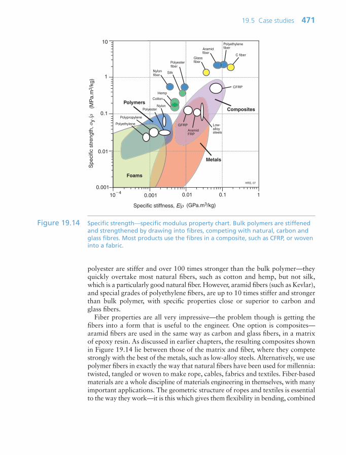
polyester are stiffer and over 100 times stronger than the bulk polymer—theyquickly overtake most natural fibers, such as cotton and hemp, but not silk,which is a particularly good natural fiber. However, aramid fibers (such as Kevlar),and special grades of polyethylene fibers, are up to 10 times stiffer and strongerthan bulk polymer, with specific properties close or superior to carbon andglass fibers.
Fiber properties are all very impressive—the problem though is getting thefibers into a form that is useful to the engineer. One option is composites—aramid fibers are used in the same way as carbon and glass fibers, in a matrixof epoxy resin. As discussed in earlier chapters, the resulting composites shownin Figure 19.14 lie between those of the matrix and fiber, where they competestrongly with the best of the metals, such as low-alloy steels. Alternatively, we usepolymer fibers in exactly the way that natural fibers have been used for millennia:twisted, tangled or woven to make rope, cables, fabrics and textiles. Fiber-basedmaterials are a whole discipline of materials engineering in themselves, with manyimportant applications. The geometric structure of ropes and textiles is essentialto the way they work—it is this which gives them flexibility in bending, combined
19.5 Case studies 471
0.001
0.1
10
Spe
cific
str
engt
h, σ
y /ρ
(
MP
a.m
3 /kg
)
Specific stiffness, E/ρ (GPa.m3/kg)
10.10.010.001104
1
0.01
HRS, 07
Polymers
Metals
Composites
Foams
GFRP
CFRP
Nylon
Low- alloysteels
Polyester
Polypropylene
Polyethylene
Cotton
Hemp
C fiberGlassfiber
Aramidfiber
Polyesterfiber
Polyethylenefiber
Nylonfiber
Silk
AramidFRP
Figure 19.14 Specific strength—specific modulus property chart. Bulk polymers are stiffenedand strengthened by drawing into fibres, competing with natural, carbon andglass fibres. Most products use the fibres in a composite, such as CFRP, or woveninto a fabric.
Ch19-H8391 1/17/07 11:39 AM Page 471
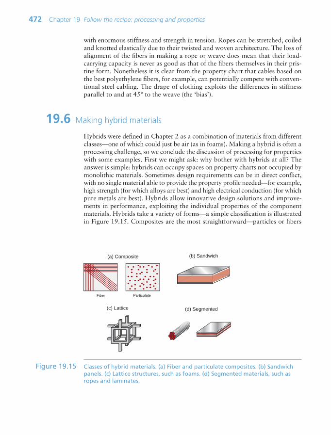
with enormous stiffness and strength in tension. Ropes can be stretched, coiledand knotted elastically due to their twisted and woven architecture. The loss ofalignment of the fibers in making a rope or weave does mean that their load-carrying capacity is never as good as that of the fibers themselves in their pris-tine form. Nonetheless it is clear from the property chart that cables based onthe best polyethylene fibers, for example, can potentially compete with conven-tional steel cabling. The drape of clothing exploits the differences in stiffnessparallel to and at 45° to the weave (the ‘bias’).
19.6 Making hybrid materials
Hybrids were defined in Chapter 2 as a combination of materials from differentclasses—one of which could just be air (as in foams). Making a hybrid is often aprocessing challenge, so we conclude the discussion of processing for propertieswith some examples. First we might ask: why bother with hybrids at all? Theanswer is simple: hybrids can occupy spaces on property charts not occupied bymonolithic materials. Sometimes design requirements can be in direct conflict,with no single material able to provide the property profile needed—for example,high strength (for which alloys are best) and high electrical conduction (for whichpure metals are best). Hybrids allow innovative design solutions and improve-ments in performance, exploiting the individual properties of the componentmaterials. Hybrids take a variety of forms—a simple classification is illustratedin Figure 19.15. Composites are the most straightforward—particles or fibers
472 Chapter 19 Follow the recipe: processing and properties
Fiber
(a) Composite
Particulate
(c) Lattice
(b) Sandwich
(d) Segmented
Figure 19.15 Classes of hybrid materials. (a) Fiber and particulate composites. (b) Sandwichpanels. (c) Lattice structures, such as foams. (d) Segmented materials, such asropes and laminates.
Ch19-H8391 1/17/07 11:39 AM Page 472

of one material embedded in another. Next are sandwich structures—skins ofhigh-performance material on a lower grade core. Lattices (random or regular)include foams and other highly porous materials, while segmented materials aremade of interlocking strands or layers of materials—ropes and cables are oftenhybrids of several types of material.
This classification is not 100% robust, since the boundaries get a bit fuzzy at theedges. For example, modern ‘nanocomposites’ are made by mixing nanometer-scale particulates into a molten metal and casting it—by Figure 19.15 this is ahybrid. However, heat treatment of steels produces an iron matrix with a finedispersion of carbides—essentially the same microstructure, also produced forstrength, yet we classify this as a metal. And at the other end of the scale, design-ing with a sandwich ‘material’ merges into designing a sandwich ‘structure’ (aski, an aircraft floor panel or an industrial door). Essentially hybrids combinematerials that are routinely available and used in their own right as bulk materials,with the bulk materials and the hybrid having definable material properties. In spite of some non-uniqueness in this definition, hybrid materials can all bethought of as some combination of component (bulk) materials plus configura-tion and scale. Configuration defines the proportions, geometric integration andshape of the components; scale defines the length scale on which they are mixed.The length scales of hybrids are mostly relatively coarse—fibers of order 1–10 µm,and the layers of laminates and sandwich panels of order 0.1–10 mm. Bulkmaterial microstructures span everything from the atomic scale (nanometers)up to the micron scale (see Figures 19.1–19.3). However, since hybrids combinethe properties of the component materials, their properties reflect microstruc-ture all the way from atomic to product scale.
Making foamsFoams extend the range of stiffness and strength axes of the property chartsdownwards by several orders of magnitude. Some foams are made by trappingbubbles in a melt and solidifying the froth as a slab. Others are made by mix-ing in chemicals which react to form a gas, injecting it into a cavity and allow-ing it to inflate in situ as the gas bubbles are formed internally. The mechanicalproperties of an ideal foam depend systematically on the relative density (thefraction of solid), as shown in Chapter 4 for Young’s modulus. In practice it isfound that the properties are also sensitive to the variability in pore size. It isimportant in processing to control the size of the largest pores, which initiatepremature failure. Metal foams and rigid polymer foams can be made to shapeand then cut and assembled into other structured materials (often as the coresof sandwich materials themselves).
Making compositesMost polymers are in fact particulate composites—bulk polymer melts towhich filler powders have been added before molding to shape. This is a hybridwhich we opt to classify as a polymer variant—largely because the scale of theadditives is very fine, almost at the scale of the polymer’s own microstructure.
19.6 Making hybrid materials 473
Ch19-H8391 1/17/07 11:39 AM Page 473
Metal–matrix composites, on the other hand, are regarded as distinct hybrids—SiC particles in aluminum alloys, for example—but they too are processedin exactly the same way as the matrix aluminum alloy. Long fiber-reinforcedpolymer composites—CFRP, GFRP and Kevlar (aramid FRP)—require dedicatedmanufacturing techniques. Their potential performance in lightweight designhas been clearly illustrated in earlier chapters, but can the ideal properties beachieved routinely in practice? The answer depends on the complexity of thecomponent geometry and the impact of joining. Composites are straightfor-ward to produce in flat panels. ‘Prepreg’ layers of partly cured resin containingunidirectional fibers are stacked, usually aligned in several directions (e.g. 0,90°, 45°) to give reasonably uniform isotropy in the properties, and curedunder pressure in an autoclave. Circular tubes are also easy to make by filamentwinding. More complex shapes are more difficult to laminate, particularly ifthe section changes in thickness. Joints are particularly troublesome. Fibercomposites cannot be welded, while drilling holes for bolts and rivets damagesthe fibers and provides stress concentrations which can initiate cracks anddelaminations around the hole. The best technique is adhesive joining, and theincreasing use of composites has stimulated the development of improved adhe-sives. Careful joint design and manufacture is necessary to avoid prematurefailure in or around the joint.
Making laminates and sandwich panelsMost interest in laminates and sandwich panels reflects the potential to exploitfiber-reinforced composites in this form—a hybrid within a hybrid. Sandwichpanels provide bending stiffness (and strength) at low weight. The lightweightcore separates the skins, to maximize the second moment of area, without con-tributing directly to the bending resistance. Good-quality adhesive joints betweenskin and core are again critical for success. Comparison of sandwich panels withmonolithic-shaped materials (such as I-beams) would normally be made oncharacteristics such as ‘flexural rigidity’ EI, as opposed to strict material prop-erties. Laminates offer another hybrid solution. Various GFRP and aluminumlaminates, such as GLARE and ARALL, have been developed for aerospacestructures, as they offer a competitive alternative to purely aluminum or compos-ite fabrication. And woods have had something of a renaissance in large-scalecivil engineering in the form of laminates such as Glulam. The laminating processdistributes the defects inherent in natural wood, reducing property variability,and enables much larger beam structures to be built. Once again, the glue betweenthe layers in all laminates is a key part of the hybrid.
19.7 Summary and conclusions
Manufacturing processes are central to achieving the target properties in amaterial. Shaping processes such as casting, molding and forming always impose
474 Chapter 19 Follow the recipe: processing and properties
Ch19-H8391 1/17/07 11:39 AM Page 474

a thermal history and often a deformation history. These do more than makethe shape—they also govern the evolution of the internal microstructure on whichproperties depend. Further processing at the surface can locally change themicrostructure and properties there, e.g. for wear resistance. And joining compo-nents together can change things further—joints often being the design-limitinglocation, or the source of disaster. So processing offers many opportunities forinnovation, together with responsibility for careful control. Metals show thegreatest versatility—not surprising with the many different elements and alloycompositions available to work with, and their inherent castability and/orformability. One class alone—ferrous alloys—covers a wide domain of the keystructural properties of strength and toughness. Other alloy systems use thesame principles of modifying chemistry, forming and heat treatment to developdifferent property profiles.
Ceramics, glasses and polymers all have some scope for variation of compo-sition and process. Blending, cross-linking and crystallinity provide modest rangesin the properties of polymers—including the elastic modulus. Most effective isthe production of fibers, taking bulk polymers into completely new territory,well beyond the performance of natural fibers. Making use of these fiber proper-ties in practical products needs imaginative hybrid construction, as composites,ropes, textiles and fabrics. Hybrids also extend to other forms—sandwich pan-els, foams and laminates. Processing again plays its part in the practicalities ofusing hybrids, with the development of high-performance adhesives receiving aboost from the drive to exploit their potential in design.
19.8 Further reading
Ashby, M.F. and Jones, D.R.H. (2005) Engineering Materials II, 3rd edition. ISBN0-7506-6381-2 (Popular treatment of material classes, and how processing affectsmicrostructure and properties.)
ASM Handbook Series (1971–2004) Volume 4, Heat Treatment; Volume 5, SurfaceEngineering; Volume 6, Welding, Brazing and Soldering; Volume 7, Powder MetalTechnologies; Volume 14, Forming and Forging; Volume 15, Casting; and Volume 16,Machining; ASM International, Metals Park, OH, USA. (A comprehensive set ofhandbooks on processing, occasionally updated, and now available online atwww.asminternational.org/hbk/index.jsp.)
Bralla, J.G. (1998) Design for Manufacturability Handbook, 2nd edition, McGraw-Hill, New York, USA. ISBN 0-07-007139-X. (Turgid reading, but a rich mine ofinformation about manufacturing processes.)
Kalpakjian, S. and Schmid, S.R. (2003) Manufacturing Processes for EngineeringMaterials, 4th edition, Prentice-Hall, Pearson Education, New Jersey, USA. ISBN 0-13-040871-9. (A comprehensive and widely used text on material processing.)
Lascoe, O.D. (1988) Handbook of Fabrication Processes, ASM International, MetalsPark, Columbus, OH, USA. ISBN 0-87170-302-5. (A reference source for fabricationprocesses.)
19.8 Further reading 475
Ch19-H8391 1/17/07 11:39 AM Page 475
476 Chapter 19 Follow the recipe: processing and properties
19.9 Exercises
Exercise E19.1 The table shows typical data for strength and fracture toughness of a selectionof copper alloys, both cast and wrought. Sketch a property chart (on log scales)and plot the data. Use the chart to answer the following:
(a) How do the cast and wrought alloys compare on fracture toughness, atcomparable strength?
(b) Rank the strengthening mechanisms (as indicated in the table) in order ofeffectiveness.
(c) Do the trends observed in (a) and (b) follow a similar pattern to alu-minum alloys (Figure 8.15)?
Exercise E19.2 The excellent specific properties of natural and artificial fibers were high-lighted in Figure 19.14. It is also of interest to explore other property combina-tions which measure performance—for example, the maximum elastic storedenergy. The table summarizes typical data for various fibers, together withsome bulk polymers and steel for comparison.
Calculate the following performance indices for the materials given: (a)maximum elastic stored energy (per unit volume), σ2
f/E; (b) maximum elasticstored energy (per unit mass), σ2
f /Eρ.Which material appears best on each criterion? Which criterion would be
more important for climbing ropes? Why is it not practical for the propertiesof fibers to be exploited to their maximum potential?
Alloy Process route Main strengthening Yield Fracture mechanisms strength (MPa) toughness (MPa.m1/2)
Pure Cu Cast None 35 105Pure Cu Hot rolled Work 80 82Bronze (10% Sn) Cast Solid solution 200 55Brass (30% Zn) Cast Solid solution 90 80Brass (30% Zn) Wrought annealed Solid solution 100 75Brass (30% Zn) Wrought Solid solution work 400 35Cu – 2% Be Wrought heat treated Precipitation 1000 17
Hemp Spider Bulk Aramid Polyester PE Nylon Alloy web silk nylon fiber fiber fiber fiber steel wire
Young’s 8 11.0 2.5 124 13 2.85 3.9 210modulus (GPa)Strength (MPa) 300 500 63 3930 784 1150 616 1330Density (kg/m3) 1490 1310 1090 1450 1390 950 1140 7800
Ch19-H8391 1/17/07 11:39 AM Page 476

19.10 Exploring design with CES 477
19.10 Exploring design with CES
Exercise E19.3 Use CES Level 3 data to explore the properties of Cu–Ni alloys. Extract datafor Young’s modulus, yield stress, fracture toughness and electrical resistiv-ity for annealed pure Cu and Ni, and a selection of alloys in between (e.g.10%, 30%, 70% Ni). Sketch how the properties vary with Ni composition(between 0 and 100%).
(Note that in CES you can plot the composition of the dominant elementon a chart axis—try plotting each property against the % Cu, selecting bothCu–Ni and Ni–Cu alloys to cover the full range, together with pure Cu andNi.)
(a) Which properties follow an approximate linear rule of mixtures betweenthe values for pure Cu and Ni?
(b) The alloys in CES are not binary Cu–Ni alloys. Which properties appearmost strongly influenced by the other alloying additions?
Exercise E19.4 Use CES Level 3 to plot the strength and fracture toughness of Mg and itsalloys. How do cast and wrought alloy variants compare?
Exercise E19.5 The records for polymers in CES include the % filler as a parameter. Plot eachof the following properties against the % filler for PA, PP and epoxy, andexplore how effective fillers are at enhancing the Young’s modulus and strengthof these polymers. How does the addition of filler affect the fracture toughnessand the price/kg?
Ch19-H8391 1/17/07 11:39 AM Page 477

This page intentionally left blank

Chapter 20Materials, processes and
the environment
Chapter contents
20.1 Introduction and synopsis 48020.2 Material consumption and its growth 48020.3 The material life cycle and criteria for
assessment 48320.4 Definitions and measurement:
embodied energy, process energyand end of life potential 484
20.5 Charts for embodied energy 49020.6 Design: selecting materials for
eco-design 49320.7 Summary and conclusions 49720.8 Appendix: some useful quantities 49820.9 Further reading 49820.10 Exercises 49920.11 Exploring design with CES 501
Power from the wind. (Image courtesy of LeicaGeosystems, Switzerland.)
Ch20-H8391 1/16/07 6:45 PM Page 479

480 Chapter 20 Materials, processes and the environment
20.1 Introduction and synopsis
The practice of engineering consumes vast quantities of materials and is dependenton a continuous supply of them. We start by surveying this consumption, empha-sizing the materials used in the greatest quantities. Increasing population and living standards cause this consumption rate to grow—something it cannot doforever. Finding ways to use materials more efficiently is a prerequisite for asustainable future.
There is a more immediate problem: present-day material usage alreadyimposes stress on the environment in which we live. The environment has somecapacity to cope with this, so that a certain level of impact can be absorbed with-out lasting damage. But it is clear that current human activities exceed this thresh-old with increasing frequency, diminishing the quality of the world in which wenow live and threatening the well-being of future generations. Design for the envi-ronment is generally interpreted as the effort to adjust our present product designefforts to correct known, measurable, environmental degradation; the time-scaleof this thinking is 10 years or so, an average product’s expected life. Design forsustainability is the longer-term view: that of adaptation to a lifestyle thatmeets present needs without compromising the needs of future generations.The time-scale here is less clear—it is measured in decades or centuries—andthe adaptation required is much greater.
20.2 Material consumption and its growth
Material consumptionSpeaking globally, we consume roughly 10 billion (1010) tonnes of engineeringmaterials per year. Figure 20.1 gives a perspective: it is a bar chart of the con-sumption of the materials used in the greatest quantities. It has some interestingmessages. On the extreme left, for calibration, are hydrocarbon fuels—oil andcoal—of which we currently consume a colossal 9 billion tonnes per year. Next,moving to the right, are metals. The scale is logarithmic, making it appear that theconsumption of steel (the first metal) is only a little greater than that of aluminum(the next); in reality, the consumption of steel exceeds, by a factor of 10, that of allother metals combined. Steel may lack the high-tech image that attaches to mate-rials like titanium, carbon-fiber reinforced composites and (most recently) nano-materials, but make no mistake, its versatility, strength, toughness, low costand wide availability are unmatched.
Polymers come next: 50 years ago their consumption was tiny; today thecombined consumption of commodity polymers polyethylene (PE), polyvinylchloride (PVC), polypropylene (PP) and polyethylene-terephthalate (PET) beginsto approach that of steel.
The really big ones, though, are the materials of the construction industry.Steel is one of these, but the consumption of wood for construction purposes
Ch20-H8391 1/16/07 6:45 PM Page 480

20.2 Material consumption and its growth 481
exceeds that of steel even when measured in tonnes per year (as in the diagram),and since it is a factor of 10 lighter, if measured in m3/year, wood totallyeclipses steel. Bigger still is the consumption of concrete, which exceeds that ofall other materials combined. The other big ones are asphalt (roads) and glass.
The last column of all illustrates things to come: it shows today’s consump-tion of carbon fiber. Just 20 years ago this material would not have crept ontothe bottom of this chart. Today its consumption is approaching that of titaniumand is growing fast.
The columns in this figure describe broad classes of materials, so—out of the160 000 materials now available—they probably include 99.9% of all consump-tion when measured in tonnes. This is important when we come to consider theimpact of materials on the environment, since impact scales with consumption.
The growth of consumptionMost materials are being consumed at a rate that is growing exponentially withtime (Figure 20.2), simply because both population and living standards growexponentially. One consequence of this is dramatized by the following state-ment: at a global growth rate of just 3% per year we will mine, process and dis-pose of more ‘stuff’ in the next 25 years than in the entire history of humanengineering (see Exercises). If the current rate of consumption in tonnes peryear is C then exponential growth means that
(20.1)ddCt
rC
100
Ann
ual w
orld
pro
duct
ion
(tonn
es/y
ear)
104
102
103
105
106
107
108
109
1010
1011
Steel
Al alloys
Zn alloysCu alloys
Pb alloys
Mg alloys
Silver
Wood
Glass
Cement
PEPPPVC
C-fiber
Asphalt
Oil and coal
Ni alloys
Gold
Ti alloys
Concrete
PET
MFA 07
Figure 20.1 The consumption of hydrocarbons (left-hand column) and of engineeringmaterials (the other columns).
Ch20-H8391 1/16/07 6:45 PM Page 481

where, for the generally small growth rates we deal with here (1–5% per year),r can be thought of as the percentage fractional rate of growth per year.Integrating over time gives
(20.2)
where C0 is the consumption rate at time t t0. The doubling time tD of con-sumption rate is given by setting C/C0 2 to give
(20.3)
After a period of stagnation, steel consumption is growing again, driven bygrowth in China; at 4% per year it doubles about every 18 years. Polymer con-sumption is rising at about 5% per year—it doubles every 14 years. During timesof boom—the 1960s and 1970s, for instance—polymer production increasedmuch faster than this, peaking at 18% per year (it doubled every 4 years).
The picture, then, is one of a global economy ever more dependent on a sup-ply of materials, almost all drawn from non-renewable resources. To managethese in a sustainable way requires an understanding of the material life cycle.We turn to this next.
tr rD elog
1002
70( )
C Cr t t
00
100exp
( )⎧⎨⎪⎪⎩⎪⎪
⎫⎬⎪⎪⎭⎪⎪
482 Chapter 20 Materials, processes and the environment
Con
sum
ptio
n ra
te C
(to
nnes
/yea
r)
Time t (years) t*t0
C0
Consumptionbetween t0 and t*
dCdt
r100
C=
Figure 20.2 Exponential growth. Consumption rate C doubles in a time td 70/r, where r isthe annual growth rate.
Ch20-H8391 1/16/07 6:45 PM Page 482
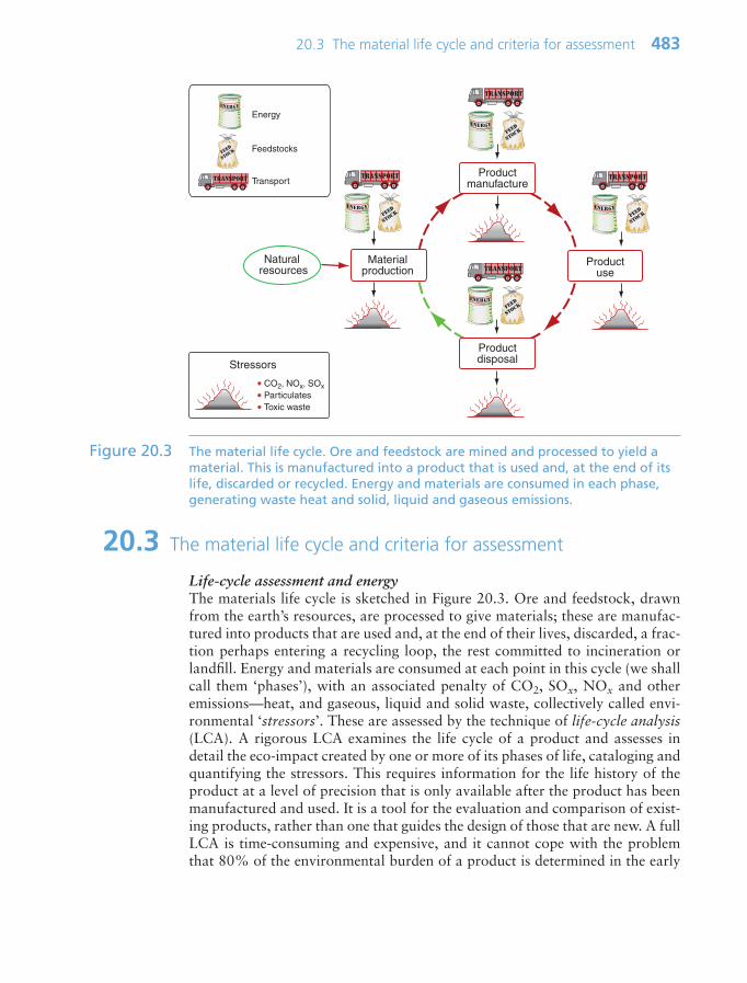
20.3 The material life cycle and criteria for assessment
Life-cycle assessment and energyThe materials life cycle is sketched in Figure 20.3. Ore and feedstock, drawnfrom the earth’s resources, are processed to give materials; these are manufac-tured into products that are used and, at the end of their lives, discarded, a frac-tion perhaps entering a recycling loop, the rest committed to incineration orlandfill. Energy and materials are consumed at each point in this cycle (we shallcall them ‘phases’), with an associated penalty of CO2, SOx, NOx and otheremissions—heat, and gaseous, liquid and solid waste, collectively called envi-ronmental ‘stressors’. These are assessed by the technique of life-cycle analysis(LCA). A rigorous LCA examines the life cycle of a product and assesses indetail the eco-impact created by one or more of its phases of life, cataloging andquantifying the stressors. This requires information for the life history of theproduct at a level of precision that is only available after the product has beenmanufactured and used. It is a tool for the evaluation and comparison of exist-ing products, rather than one that guides the design of those that are new. A fullLCA is time-consuming and expensive, and it cannot cope with the problemthat 80% of the environmental burden of a product is determined in the early
20.3 The material life cycle and criteria for assessment 483
Materialproduction
Productmanufacture
Productuse
Productdisposal
Natural resources
CO2, NOx, SOxParticulatesToxic waste
Stressors
Energy
Feedstocks
Transport
Figure 20.3 The material life cycle. Ore and feedstock are mined and processed to yield amaterial. This is manufactured into a product that is used and, at the end of itslife, discarded or recycled. Energy and materials are consumed in each phase,generating waste heat and solid, liquid and gaseous emissions.
Ch20-H8391 1/16/07 6:45 PM Page 483
stages of design, when many decisions are still fluid. This has led to the devel-opment of more approximate ‘streamline’ LCA methods that seek to combineacceptable cost with sufficient accuracy to guide decision-making, the choice ofmaterials being one of these decisions. But even then there is a problem: adesigner, seeking to cope with many interdependent decisions that any designinvolves, inevitably finds it hard to know how best to use data of this type.How are CO2 and SOx emissions to be balanced against resource depletion,toxicity or ease of recycling?
This perception has led to efforts to condense the eco-information about amaterial production into a single measure or indicator, normalizing andweighting each source of stress to give the designer a simple, numeric ranking.The use of a single-valued indicator is criticized by some. The grounds for crit-icism are that there is no agreement on normalization or weighting factors, andthat the method is opaque since the indicator value has no simple physical sig-nificance. But on one point there is international agreement: the Kyoto Protocolof 1997 committed the developed nations that signed it to progressively reducecarbon emissions, meaning CO2. At the national level the focus is more onreducing energy consumption, but since this and CO2 production are closelyrelated, they are nearly equivalent. Thus, there is a certain logic in basingdesign decisions on energy consumption or CO2 generation; they carry moreconviction than the use of a more obscure indicator. We shall follow this route,using energy as our measure. Before doing this, some definitions.
20.4 Definitions and measurement: embodied energy, processenergy and end of life potential
Embodied energy Hm and CO2 footprintThe embodied energy of a material is the energy that must be committed to cre-ate 1 kg of usable material—1 kg of steel stock, or of PET pellets, or of cementpowder, for example—measured in MJ/kg. The CO2 footprint is the associatedrelease of CO2, in kg/kg. It is tempting to try to estimate embodied energy viathe thermodynamics of the processes involved—extracting aluminum from itsoxide, for instance, requires the provision of the free energy of oxidation to lib-erate it. This much energy must be provided, it is true, but it is only the begin-ning. The thermodynamic efficiencies of processes are low, seldom reaching50%. Only part of the output is usable—the scrap fraction ranges from a fewpercent to more than 10%. The feedstocks used in the extraction or productionthemselves carry embodied energy. Transport is involved. The production plantitself has to be lit, heated and serviced. And if it is a dedicated plant, one that isbuilt for the sole purpose of making the material or product, there is an ‘energymortgage’—the energy consumed in building the plant in the first place.
Embodied energies are more properly assessed by input–output analysis. Forexample, for a material such as ingot iron, cement powder or PET granules, theembodied energy/kg is found by monitoring over a fixed period of time the total
484 Chapter 20 Materials, processes and the environment
Ch20-H8391 1/16/07 6:45 PM Page 484

energy input to the production plant (including that smuggled in, so to speak, asembodied energy of feedstock) and dividing this by the quantity of usable mate-rial shipped out of the plant. The upper part of Figure 20.4 shows, much simpli-fied, the inputs to a PET production facility: oil derivatives such as naphtha andother feedstock, direct power (which, if electric, is generated with a productionefficiency of about 34%), and the energy of transporting the feedstock to thefacility. The plant has an hourly output of usable PET granules. The embodiedenergy of the PET, (Hm)PET, with usual units of MJ/kg, is then given by
The processing energy Hp associated with a material is the energy, in MJ, usedto shape, join and finish 1 kg of the material to create a component or product.Thus polymers, typically, are molded or extruded; metals are cast, forged ormachined; ceramics are shaped by powder methods. A characteristic energy perkg is associated with each of these. Continuing with the PET example, the gran-ules now become the input (after transportation) to a facility for blow-moldingPET bottles for water, as shown in the lower part of Figure 20.4. There is no
( )Hm PET
Energies entering plant per hour
Ma
∑sss of PET granules produced per hour
20.4 Definitions and measurement 485
OI L
CO2NOXSOX
Oil derivatives
Plantenergy
PET pellets (with embodied
energy)
Bottle
molding
plant
CO
TRUCKING
TRUCKING
Transport
CO2NOXSOX
CO
PET
production
plant
Bottles(with embodied energy)
Figure 20.4 An input–output diagram for PET production (giving the embodied energy/kgof PET) and for bottle production (giving the embodied energy/bottle).
Ch20-H8391 1/16/07 6:45 PM Page 485

need to list the inputs again—they are broadly the same, the PET itself bringingwith it its embodied energy (Hm)PET. The output of the analysis is the energycommitted per bottle produced.
There are many more steps before the bottle reaches a consumer and isdrunk: collection, filtration and monitoring of the water, transportation ofwater and bottles to bottling plant, labeling, delivery to central warehouse, dis-tribution to retailers and refrigeration prior to sale. All have energy inputs,which, when totalled, give the energy cost of as simple a thing as a plastic bottle of cold water.
The end-of-life potential summarizes the possible utility of the material atlife’s end: the ability to be recycled back into the product from which it came,the lesser ability to be down-cycled into a lower-grade application, the abilityto be biodegraded into usable compost, the ability to yield energy by controlledcombustion and, failing all of these, the ability to be buried as landfill withoutcontaminating the surrounding land then or in the future.
Recycling: ideals and realitiesWe buy, use and discard paper, packaging, cans, bottles, television sets, com-puters, furniture, tires, cars, even buildings. Why not retrieve the materials theycontain and use them again? What could be simpler?
If you think that, think again. First, some facts. There are (simplifying again)two sorts of ‘scrap’, by which we mean material with recycle potential. In-housescrap is the off-cuts, ends and bits left in a material production facility when the usable material is shipped out. Here ideals are realized: almost 100% isrecycled, meaning that it goes back into the primary production loop. But oncea material is released into the outside world the picture changes. It is processedto make parts that may be small, very numerous and widely dispersed; it isassembled into products that contain many other materials; it may be painted,printed or plated; and its subsequent use contaminates it further. To reuse it, itmust be collected (not always easy), separated from other materials, identified,decontaminated, chopped and processed. Collection is time-intensive and thismakes it expensive. Imperfect separation causes problems: even a little copperor tin damages the properties of steel; residual iron embrittles aluminum; heavymetals (lead, cadmium, mercury) are unacceptable in many alloys; PVC con-tamination renders PET unusable, and dyes, water and almost any alien plasticrenders a polymer unacceptable for its original demanding purpose, mean-ing that it can only be used in less demanding applications (a fate known as‘down-cycling’).
Despite these difficulties, recycling can be economic, both in cash and energyterms. This is particularly so for metals: the energy commitment per kg for recycledaluminum is about one-tenth of that for virgin material; that for steel is aboutone-third. Some inevitable contamination is countered by addition of virginmaterial to dilute it. Metal recycling is both economic and makes importantcontributions to the saving of energy.
486 Chapter 20 Materials, processes and the environment
Ch20-H8391 1/16/07 6:45 PM Page 486
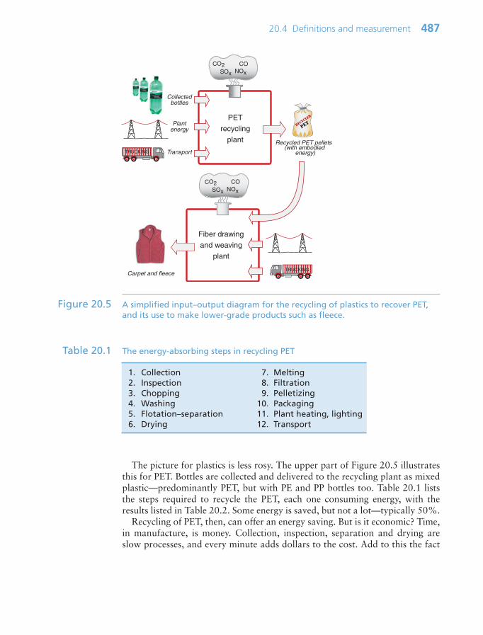
The picture for plastics is less rosy. The upper part of Figure 20.5 illustratesthis for PET. Bottles are collected and delivered to the recycling plant as mixedplastic—predominantly PET, but with PE and PP bottles too. Table 20.1 liststhe steps required to recycle the PET, each one consuming energy, with theresults listed in Table 20.2. Some energy is saved, but not a lot—typically 50%.
Recycling of PET, then, can offer an energy saving. But is it economic? Time,in manufacture, is money. Collection, inspection, separation and drying areslow processes, and every minute adds dollars to the cost. Add to this the fact
20.4 Definitions and measurement 487
CO2NOxSOx
Collectedbottles
Plantenergy
Recycled PET pellets (with embodied
energy)
Fiber drawing
and weaving
plant
CO
TRUCKING
TRUCKING
Transport
CO2NOxSOx
CO
PET
recycling
plant
Carpet and fleece
Figure 20.5 A simplified input–output diagram for the recycling of plastics to recover PET,and its use to make lower-grade products such as fleece.
1. Collection 7. Melting2. Inspection 8. Filtration3. Chopping 9. Pelletizing4. Washing 10. Packaging5. Flotation–separation 11. Plant heating, lighting6. Drying 12. Transport
Table 20.1 The energy-absorbing steps in recycling PET
Ch20-H8391 1/16/07 6:45 PM Page 487
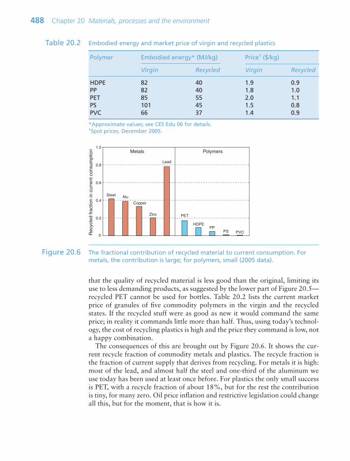
that the quality of recycled material is less good than the original, limiting itsuse to less demanding products, as suggested by the lower part of Figure 20.5—recycled PET cannot be used for bottles. Table 20.2 lists the current marketprice of granules of five commodity polymers in the virgin and the recycledstates. If the recycled stuff were as good as new it would command the sameprice; in reality it commands little more than half. Thus, using today’s technol-ogy, the cost of recycling plastics is high and the price they command is low, nota happy combination.
The consequences of this are brought out by Figure 20.6. It shows the cur-rent recycle fraction of commodity metals and plastics. The recycle fraction isthe fraction of current supply that derives from recycling. For metals it is high:most of the lead, and almost half the steel and one-third of the aluminum weuse today has been used at least once before. For plastics the only small successis PET, with a recycle fraction of about 18%, but for the rest the contributionis tiny, for many zero. Oil price inflation and restrictive legislation could changeall this, but for the moment, that is how it is.
488 Chapter 20 Materials, processes and the environment
Polymer Embodied energy* (MJ/kg) Price† ($/kg)
Virgin Recycled Virgin Recycled
HDPE 82 40 1.9 0.9PP 82 40 1.8 1.0PET 85 55 2.0 1.1PS 101 45 1.5 0.8PVC 66 37 1.4 0.9
Table 20.2 Embodied energy and market price of virgin and recycled plastics
*Approximate values; see CES Edu 06 for details.†Spot prices, December 2005.
Steel Alu
Zinc
Copper
Lead
PET
HDPEPP
PS PVC0
0.4
0.2
0.6
1.0
0.8
Rec
ycle
d fr
actio
n in
cur
rent
con
sum
ptio
n Metals Polymers
Figure 20.6 The fractional contribution of recycled material to current consumption. Formetals, the contribution is large; for polymers, small (2005 data).
Ch20-H8391 1/16/07 6:45 PM Page 488
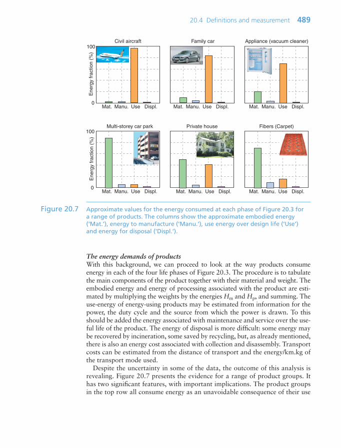
The energy demands of productsWith this background, we can proceed to look at the way products consumeenergy in each of the four life phases of Figure 20.3. The procedure is to tabulatethe main components of the product together with their material and weight. Theembodied energy and energy of processing associated with the product are esti-mated by multiplying the weights by the energies Hm and Hp, and summing. Theuse-energy of energy-using products may be estimated from information for thepower, the duty cycle and the source from which the power is drawn. To thisshould be added the energy associated with maintenance and service over the use-ful life of the product. The energy of disposal is more difficult: some energy maybe recovered by incineration, some saved by recycling, but, as already mentioned,there is also an energy cost associated with collection and disassembly. Transportcosts can be estimated from the distance of transport and the energy/km.kg ofthe transport mode used.
Despite the uncertainty in some of the data, the outcome of this analysis isrevealing. Figure 20.7 presents the evidence for a range of product groups. Ithas two significant features, with important implications. The product groupsin the top row all consume energy as an unavoidable consequence of their use
20.4 Definitions and measurement 489
Mat. Manu. Use Displ.
Private house
Ene
rgy
frac
tion
(%)
0
100
Mat. Manu. Use Displ.
Multi-storey car park
Mat. Manu. Use Displ.
Ene
rgy
frac
tion
(%)
0
100Civil aircraft
Mat. Manu. Use Displ.
Family car
Mat. Manu. Use Displ.
Appliance (vacuum cleaner)
Mat. Manu. Use Displ.
Fibers (Carpet)
Figure 20.7 Approximate values for the energy consumed at each phase of Figure 20.3 for a range of products. The columns show the approximate embodied energy(‘Mat.’), energy to manufacture (‘Manu.’), use energy over design life (‘Use’)and energy for disposal (‘Displ.’).
Ch20-H8391 1/16/07 6:45 PM Page 489

and for these the use-phase overwhelmingly dominates the life energy. Theproducts in the bottom row depend less heavily on energy but are materialintensive; for these it is the embodied energy of the material that dominates. Iflarge changes are to be achieved, it is the dominant phase that must be the firsttarget; when the differences are as great as those shown here, a reduction in theothers makes little impact on the total, and the precision of the data for Hm andHp is not the issue—an error of a factor of 2 changes the outcome very little. Itis in the nature of those who conduct detailed LCA studies to wish to do sowith precision, and better data is always a desirable goal. But engineers anddesigners need the ability to move forward without it, recognizing that precisejudgements can be drawn from imprecise data.
20.5 Charts for embodied energy
Bar charts for embodied energyFigures 20.8 and 20.9 show the embodied energy per kg and per m3 for materials.When compared per unit mass, metals, particularly steels, appear as attractivechoices, demanding much less energy than polymers. But when compared on avolume basis, the ranking changes and polymers lie lower than metals. The light
490 Chapter 20 Materials, processes and the environment
Em
bodi
ed e
nerg
y/kg
, MJ/
kg
1
10
102
103
MFA 07 Metals Polymers Ceramics Hybrids
Ti alloys
Stainless steels
LA steels
Carbon steels
Al alloys
Mg alloys
PEEVAPP
Nylon
PC
PEEK
PET
PTFE
PMMA
ABS
PVC
ConcreteWood
Plywood
GFRP
Polymer foams
Ceramic foams
CFRP
Metal foams
Cement
Brick
Stone
Lead alloys
PSNi alloys
Cast irons
Naturalrubber
Epoxy Alumina
Zirconia
Aluminum nitride
Silica glass
Soda glass
Metal–matrix composites
Figure 20.8 Bar chart of embodied energy of basic materials by weight. By this measurepolymers are more energy intensive than many metals
Ch20-H8391 1/16/07 6:45 PM Page 490

alloys based on aluminum, magnesium and titanium are particularly demanding,with energies that are high by either measure. This prompts the question: whatmeasure should we choose to make meaningful comparisons if we wish to mini-mize the embodied energy of a product? The answer is the same as the one weused with the objectives of minimizing mass or cost: it is to minimize embodiedenergy per unit of function. To do that we need the next two charts.
Property charts for embodied energy in structural designEarlier chapters discussed the property trade-offs in problems of structural design.The function of the design might be, for example, to support a load without too much deflection, or without failure, while minimizing the mass. For this,modulus–density or strength–density were used. If the objective becomes mini-mizing the energy embodied in the material of the product while providingstructural functionality, we need equivalent charts for these.
Figures 20.10 and 20.11 are a pair of materials selection charts for minimiz-ing energy Hm per unit stiffness and strength. The first shows modulus E plot-ted against Hmρ; the guidelines give the slopes for three of the commonestperformance indices. The second shows strength σy plotted against Hmρ; again,guidelines give the slopes. The two charts give survey data for minimum energydesign. They are used in exactly the same way as the E–ρ and σy–ρ charts forminimum mass design.
20.5 Charts for embodied energy 491
Em
bodi
ed e
nerg
y/m
3 , M
J/m
3
103
104
105
107
106
Metals Polymers Ceramics Hybrids
Ti alloys
Stainless steels
LA steels
Carbon steels
Al alloysMg alloys
PE
EVA
PP
NylonPC
PEEK
PET
PTFE
PMMA
ABSPVC
Concrete
Wood
MFA07
Plywood
GFRP
Polymer foams
Ceramic foams
CFRP
Metalfoams
Cement
Brick
Stone
Lead alloys
PS
Ni alloys
Cast irons
Naturalrubber
Epoxy
Alumina
Zirconia
Aluminum nitride
Silica glass
Soda glass
Metal–matrix composites
Figure 20.9 Bar chart of embodied energy of basic materials by volume. By this measurepolymers are less energy intensive than any metal.
Ch20-H8391 1/16/07 6:45 PM Page 491

492 Chapter 20 Materials, processes and the environment
You
ng’s
mod
ulus
, E (
GP
a)
Embodied energy per cubic meter, Hm.ρ (MJ/m3)
0.01
10
0.1
1
102
103
102 103 104 105 106 107
E1/3
E1/2
EHmρ
Guidelines for minimum energy
design
Hmρ
Hmρ
Foams
Polymers
Metals
Technicalceramics
CompositesLead alloys
W alloys
Carbon steels
Ti alloys
Mg alloys
CFRP
GFRP
Al alloys
Rigid polymer foams
Flexible polymer foams
Ni alloys
Cu alloys
Zinc alloys
PS
PTFE
PC
Cork
Silicone elastomers
Concrete
Al2O3
BiCModulus–Energy/m3
B4C
PP
EVA
Polyurethane
Leather
Non-technical ceramics
MFA, 07
Castirons
WC
Soda glass
Silica glass
Silicon
StoneBrick
ABS
Epoxies
Ionomers
AlN
Stainless steels
PEEK
PE Polyurethanes
Acetal
Borosilicate glass
Nylons
PVCPET
Phenolics
Elastomers
Wood // to grain
Wood to grain
Bamboo
Natural materials
Figure 20.10 The modulus–embodied energy chart made with the CES software. It is theequivalent of the Eρ chart of Figure 4.6 and is used in the same way.
Embodied energy per cubic meter, Hm·ρ (MJ/m3)102 103 104 105 106 107
Str
engt
h, σ
y (
MP
a)
0.01
10
0.1
1
102
103
104
σy1/2σy
2/3σy
Guidelines for minimum energy
design
Hm ρ Hm ρ Hmρ
Foams
Polymers and elastomers
Metals
Technicalceramics
Lead alloys
W alloys
Carbon steels
Ti alloys
Mg alloys
CFRP
GFRP
Al alloys
Rigid polymer foams
Flexible polymer foams
Cu alloys
Zinc alloys
PS
PTFE
Cork
Silicone elastomers
Concrete
Al2O3 SiCSi3N4
Strength–Energy/m3
PP
NeopreneLeather
Non-technical ceramics
Cast irons
WC
Silica glass
Stone
Brick
ABS
Butyl rubber
AlN
Stainless steels
PEEKPE
Ni alloys
Sodaglass
MFA, 07
Composites
Wood to grain
Bamboo
Naturalmaterials
Wood // to grain
Figure 20.11 The strength–embodied energy chart made with the CES software. It is theequivalent of the σyρ chart of Figure 6.6 and is used in the same way.
Ch20-H8391 1/16/07 6:45 PM Page 492

20.6 Design: selecting materials for eco-design
For selection of materials in environmentally responsible design we must firstask: which phase of the life cycle of the product under consideration makes thelargest impact on the environment? The answer guides the effective use of thedata in the way shown in Figure 20.12.
The material production phaseIf material production consumes more energy than the other phases of life, itbecomes the first target. Drink containers provide an example: they consumematerials and energy during material extraction and container production, but,apart from transport and possible refrigeration, not thereafter. Here, selectingmaterials with low embodied energy and using less of them are the ways for-ward. Figure 20.7 made the point that large civil structures—buildings, bridges,roads—are material intensive. For these the embodied energy of the materialsis the largest commitment. For this reason architects and civil engineers con-cern themselves with embodied energy as well as the thermal efficiency of theirstructures.
The product manufacture phaseThe energy required to shape a material is usually much less than that to createit in the first place. Certainly it is important to save energy in production. But
20.6 Design: selecting materials for eco-design 493
Assess energy use over life
Materials
Manufacture
Use
Disposal
Ene
rgy
Materials
Minimize
embodied energy
CO 2/kg
Non-sustainable materials
Manufacture Use Disposal
Minimize
process energy
CO 2/kg
Local pollution
Minimize
mass
heat losses
electrical losses
Select
Non-toxic materials
Materials that can be recycled
Strategy
Figure 20.12 Rational use of the database starts with an analysis of the phase of life to betargeted. The decision then guides the method of selection to minimize theimpact of the phase on the environment.
Ch20-H8391 1/16/07 6:45 PM Page 493
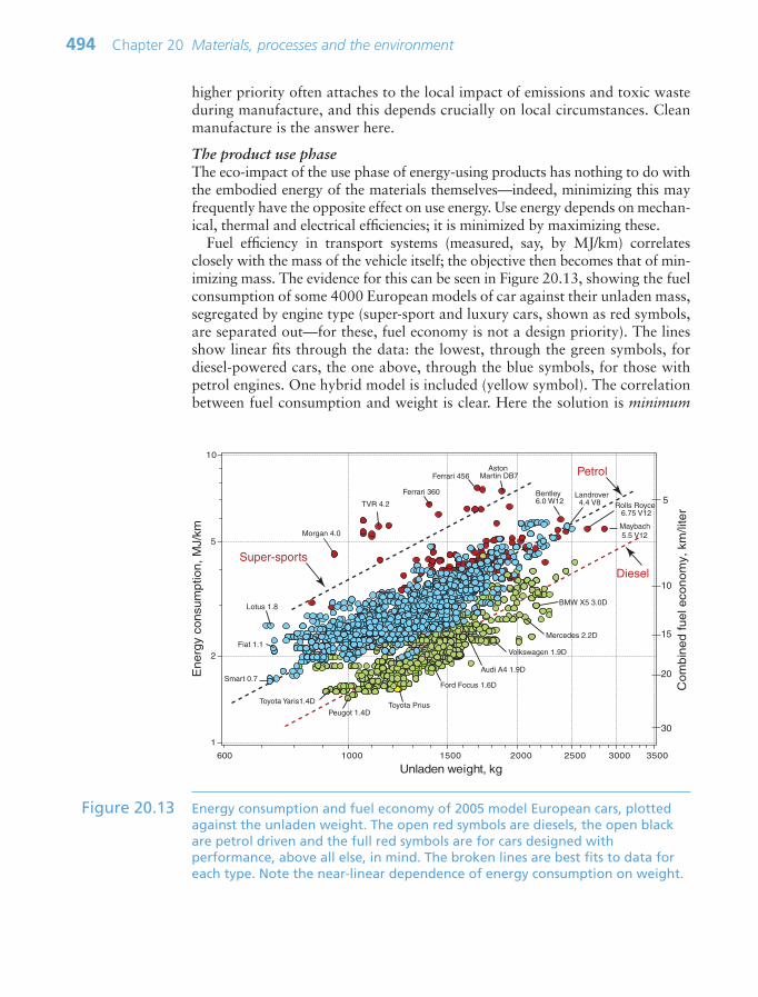
higher priority often attaches to the local impact of emissions and toxic wasteduring manufacture, and this depends crucially on local circumstances. Cleanmanufacture is the answer here.
The product use phaseThe eco-impact of the use phase of energy-using products has nothing to do withthe embodied energy of the materials themselves—indeed, minimizing this mayfrequently have the opposite effect on use energy. Use energy depends on mechan-ical, thermal and electrical efficiencies; it is minimized by maximizing these.
Fuel efficiency in transport systems (measured, say, by MJ/km) correlatesclosely with the mass of the vehicle itself; the objective then becomes that of min-imizing mass. The evidence for this can be seen in Figure 20.13, showing the fuelconsumption of some 4000 European models of car against their unladen mass,segregated by engine type (super-sport and luxury cars, shown as red symbols,are separated out—for these, fuel economy is not a design priority). The linesshow linear fits through the data: the lowest, through the green symbols, fordiesel-powered cars, the one above, through the blue symbols, for those withpetrol engines. One hybrid model is included (yellow symbol). The correlationbetween fuel consumption and weight is clear. Here the solution is minimum
494 Chapter 20 Materials, processes and the environment
Unladen weight, kg
1
2
5
10
1000 1500 2000 2500 3000 3500600
En
erg
y co
nsu
mp
tion
, M
J/km
Co
mb
ine
d f
ue
l eco
no
my,
km
/lite
r
Diesel
Petrol
Super-sports
5
10
15
20
30
Toyota Prius
Smart 0.7
Peugot 1.4D
Ford Focus 1.6D
Bentley 6.0 W12
Maybach 5.5 V12
Rolls Royce 6.75 V12
Landrover 4.4 V8
BMW X5 3.0D
Volkswagen 1.9D
Mercedes 2.2D
Lotus 1.8
Audi A4 1.9D
Toyota Yaris1.4D
Ferrari 456 Aston Martin DB7
TVR 4.2
Ferrari 360
Morgan 4.0
Fiat 1.1
Figure 20.13 Energy consumption and fuel economy of 2005 model European cars, plottedagainst the unladen weight. The open red symbols are diesels, the open blackare petrol driven and the full red symbols are for cars designed withperformance, above all else, in mind. The broken lines are best fits to data foreach type. Note the near-linear dependence of energy consumption on weight.
Ch20-H8391 1/16/07 6:45 PM Page 494
mass design, discussed extensively in earlier chapters; it is just as relevant toeco-design as to performance-driven design.
Energy efficiency in refrigeration or heating systems is achieved by minimiz-ing the heat flux into or out of the system; the objective is then that of minimizingthermal conductivity or thermal inertia. Energy efficiency in electrical genera-tion, transmission and conversion is maximized by minimizing the ohmic lossesin the conductor; here the objective is to minimize electrical resistance whilemeeting necessary constraints on strength, cost, etc. Material selection to meetthese objectives is well documented in other chapters and the texts listed under‘Further reading’.
The product disposal phaseThe environmental consequences of the final phase of product life have manyaspects. The ideal is summarized in the following guidelines:
• Avoid toxic materials such as heavy metals and organometallic compoundsthat, in landfill, cause long-term contamination of soil and groundwater.
• Examine the use of materials that cannot be recycled, since recycling cansave both material and energy, but keep in mind the influence they have onthe other phases of life.
• Seek to maximize recycling of materials for which this is possible, eventhough recycling may be difficult to achieve for the reasons already discussed.
• When recycling is impractical seek to recover energy by controlled combustion.• Consider the use of materials that are biodegradable or photo-degradable,
although these are ineffectual in landfill because the anaerobic conditionswithin them inhibit rather than promote degradation.
Implementing this requires information for toxicity, potential for recycling,controlled combustion and biodegradability. The CES software provides sim-ple checks of each of these.
Case study: crash barriersBarriers to protect driver and passengers of road vehicles are of two types: thosethat are static (the central divider of a freeway, for instance) and those that move(the fender of the vehicle itself) (Figure 20.14). The static type lines tens of thou-sands of miles of road. Once in place they consume no energy, create no CO2 andlast a long time. The dominant phases of their life in the sense of Figure 20.7 arethose of material production and manufacture. The fender, by contrast, is part ofthe vehicle; it adds to its weight and thus to its fuel consumption. The dominantphase here is that of use. This means that, if eco-design is the objective, the crite-ria for selecting materials for the two sorts of barrier will differ.
The function of a barrier is to transfer load from the point of impact to thesupport structure, where reaction from the foundation or from crush elementsin the vehicle support or absorb it. To do this the material of the barrier musthave adequate strength, σy, and the ability to be shaped and joined cheaply, and(thinking of the disposal phase of life) recyclable. That for the car fender must
20.6 Design: selecting materials for eco-design 495
Ch20-H8391 1/16/07 6:45 PM Page 495

meet these constraints with minimum mass, since this will reduce the use energy.As we know from Chapter 7, this means materials with high values of the index
where σy is the tensile strength and ρ is its density. For the static barrier embod-ied energy, not weight, is the problem. If we change the objective to that of min-imum embodied energy, we require materials with large values of
where Hm is the embodied energy per kg of material.The chart of Figure 7.8 guides selection for the mobile barrier, where we seek
strength at low weight. CFRPs excel by this criterion, but they are not recyc-lable. Heavier, but recyclable, are alloys of magnesium, titanium and alu-minum. Ceramics are excluded both by their brittleness and the difficulty ofshaping and joining them.
The chart of Figure 20.11 guides the selection for static barriers, where we seekstrength at low embodied energy. The index M2 is plotted in Figure 20.15. Thechart shows that embodied energy per unit strength (leaving ceramics asidebecause of brittleness) is minimized by making the barrier from carbon steel, castiron or wood; nothing else comes close.
MH2 σ
ρy
m
M1 σ
ρy
496 Chapter 20 Materials, processes and the environment
W
Figure 20.14 Two crash barriers, one static, the other—the fender—attached to somethingthat moves. Different eco-criteria are needed for each.
Ch20-H8391 1/16/07 6:45 PM Page 496

Stiffness-limited design is treated in a similar way. Achieving it at minimummass was the subject of Chapters 4 and 5. To do so at minimum embodiedenergy just requires that ρ is replaced by Hmρ.
20.7 Summary and conclusions
Rational selection of materials to meet environmental objectives starts by identi-fying the phase of product life that causes greatest concern: production, manufac-ture, use or disposal. Dealing with all of these requires data not only for theobvious eco-attributes (energy, CO2 and other emissions, toxicity, ability to berecycled, and the like) but also data for mechanical, thermal, electrical and chem-ical properties. Thus, if material production is the phase of concern, selection isbased on minimizing the embodied energy or the associated emissions (CO2 pro-duction, for example). But if it is the use phase that is of concern, selection isbased instead on low weight, or excellence as a thermal insulator, or as an electri-cal conductor while meeting other constraints on stiffness, strength, cost, etc. Thecharts of this book give guidance in meeting these constraints and objectives. TheCES databases provide data and tools that allow more sophisticated selection.
20.7 Summary and conclusions 497
Embodied energy per cubic meter, Hm·ρ (MJ/m3)102 103 104 105 106 107
Str
engt
h, σ
y (
MP
a)
0.01
10
0.1
1
102
103
104
σy1/2σy
2/3σy
Guidelines for minimum energy
design
Hmρ Hmρ Hmρ
Foams
Polymers and elastomers
Metals
Technicalceramics
Lead alloys
W alloys
Carbon steels
Ti alloys
Mg alloys
CFRP
GFRP
Al alloys
Rigid polymer foams
Flexible polymer foams
Cu alloys
Zinc alloys
PS
PTFE
Cork
Silicone elastomers
Concrete
Al2O3 SiCSi3N4
Strength–Energy/m3
PP
NeopreneLeather
Non-technical ceramics
Cast irons
WC
Silica glass
Stone
Brick
ABS
Butyl rubber
AlN
Stainless steels
PEEKPE
Ni alloys
Sodaglass
MFA, 07
Composites
Wood to grain
Bamboo
Naturalmaterials
Wood // to grain
SSABS
SodS
Stainless steel
tes
WoW
Figure 20.15 The selection of materials for strength at minimum embodied energy. The best choices (rejecting ceramics because they are brittle) are cast iron, steel and wood.
Ch20-H8391 1/16/07 6:45 PM Page 497

20.8 Appendix: some useful quantities
Energy contents of fuels
• Coal, lignite 15–19 MJ/kg• Coal, anthracite 31–34 MJ/kg• Oil 11.69 kWh/liter 47.3 MJ/kg• Gas 10.42 kWh/m3
• LPG 13.7 kWh/liter 46.5–49.6 MJ/kg
Approximate energy requirements of transport systems in MJ pertonne-km
• Sea freight 0.11• Barge (river freight) 0.83• Rail freight 0.86• Truck 0.9–1.5, depending on size of truck (large are more
economic)• Air freight 8.3–15, depending on type and size of plane
Conversion factors
• 1 BthU 1.06 kJ• 1 kWh/kg (sometimes written kW/kg/h) 3.6 MJ/kg• A barrel of oil 42 US gallons 159 liters 138 kg 6210 MJ• At $50 per barrel, a dollar buys 124 MJ
20.9 Further reading
Ashby, M.F. (2005) Materials Selection in Mechanical Design, 3rd edition, Butterworth-Heinemann, Oxford, UK. ISBN 0-7506-6168-2. (A more advanced text developing theideas presented here.)
Brundlandt, D. (1987) Report of the World Commission on the Environment andDevelopment, Oxford University Press, Oxford, UK. ISBN 0-19-282080-X. (A muchquoted report that introduced the need and potential difficulties of ensuring a sustain-able future.)
Dieter, G.E. (1991) Engineering Design, A Materials and Processing Approach, 2nd edi-tion, McGraw-Hill, New York, USA. ISBN 0-07-100829-2. (A well-balanced andrespected text focusing on the place of materials and processing in technical design.)
Goedkoop, M., Effting, S. and Collignon, M. (2000) The Eco-indicator 99: A DamageOriented Method for Life Cycle Impact Assessment, Manual for Designers (14 April2000), http://www.pre.nl. (An introduction to eco-indicators, a technique for rollingall the damaging aspects of material production into a single number.)
498 Chapter 20 Materials, processes and the environment
Ch20-H8391 1/16/07 6:45 PM Page 498

Graedel, T.E. (1998) Streamlined Life-cycle Assessment, Prentice-Hall, New Jersey,USA. ISBN 0-13-607425-1. (An introduction to LCA methods and ways of streamlin-ing them.)
Kyoto Protocol (1997) United Nations, Framework Convention on Climate Change.Document FCCC/CP1997/7/ADD.1 (http://cop5.unfccc.de) O) 14040/14041/14042/14043, ‘Environmental management—life cycle assessment’ and subsections, Geneva,Switzerland. (The international consensus on combating climate change.)
20.10 Exercises 499
20.10 Exercises
Exercise E20.1 What is meant by embodied energy per kilogram of a metal? Why does it differ from the thermodynamic energy of formation of the oxide, sulfide orsilicate from which it was extracted?
Exercise E20.2 What is meant by the process energy per kilogram for casting a metal? Whydoes it differ from the latent heat of melting of the metal?
Exercise E20.3 Why is the recycling of metals more successful than that of polymers?
Exercise E20.4 The world consumption rate of CFRP is rising at 8% per year. How long doesit take to double?
Exercise E20.5 Prove the statement made in the text that, ‘at a global growth rate of just 3% per year we will mine, process and dispose of more ‘stuff’ in the next 25 years than in the entire history of human engineering’. For the purpose ofyour proof, assume consumption started with the dawn of the industrial rev-olution, 1750.
Exercise E20.6 Which phase of life would you expect to be the most energy intensive (in thesense of consuming fossil fuel) for the following products:
• A toaster.• A two-car garage.• A bicycle.• A motorbike.• A wind turbine.• A ski lift.
Indicate, in each case, your reasoning in one sentence.
Exercise E20.7 Show that the index for selecting materials for a strong panel, loaded inbending, with the minimum embodied energy content is:
MH
σ
ρy
m
Ch20-H8391 1/16/07 6:45 PM Page 499
500 Chapter 20 Materials, processes and the environment
Exercise E20.8 Use the chart E–Hmρ chart of Figure 20.10 to find the metal with a modulusE greater than 100 GPa and the lowest embodied energy per unit volume.
Exercise E20.9 Use the chart of σy–Hmρ (Figure 20.11) to find material for strong panelswith minimum embodied energy per unit volume.
Exercise E20.10 Car fenders used to be made of steel. Most cars now have extruded alu-minum or glass-reinforced polymer fenders. Both materials have a muchhigher embodied energy than steel. Take the mass of a steel bumper to be20 kg and that of an aluminum one to be 14 kg; a bumper-set (two bumpers)weighs twice as much. Find an equation for the energy consumption inMJ/km as a function of mass for petrol engine cars using the data plotted inFigure 20.13.
(a) Work out how much energy is saved by changing the bumper-set of a1500 kg car from steel to aluminum.
(b) Calculate whether, over an assumed life of 200 000 km, the switch fromsteel to aluminum has saved energy. You will find the embodied ener-gies of steel and aluminum in the CES Level 2 database. Ignore the dif-ferences in energy in manufacturing the two bumpers—it is small. (Theenergy content of gasoline is 44 MJ/litre.)
(c) The switch from steel to aluminum increases the price of the car by $60. Using current pump prices for gasoline, work out whether, over theassumed life, it is cheaper to have the aluminum fender or the steel one.
Ch20-H8391 1/16/07 6:45 PM Page 500

Container type Material Mass (g) Embodied energy (MJ/kg)
PET 400 ml bottle PET 25 84PE 1 liter milk bottle High-density PE 38 80Glass 750 ml bottle Soda glass 325 14Al 440 ml can 5000 series Al alloy 20 200Steel 440 ml can Plain carbon steel 45 23
20.11 Exploring design with CES 501
20.11 Exploring design with CES
Exercise E20.11 Rank the three common commodity materials Low carbon steel, Age hard-ening aluminum alloy and Polyethylene by embodied energy/kg and embod-ied energy/m3, using data drawn from Level 2 of the CES Edu database (use the means of the ranges given in the databases). Materials in productsperform a primary function—providing stiffness, strength, heat transfer andthe like. What is the appropriate measure of embodied energy for a givenfunction?
Exercise E20.12 Plot a bar chart for the embodied energies of metals and compare it withone for polymers, on a ‘per unit yield strength’ basis, using CES. You willneed to use the ‘Advanced’ facility in the axis-selection window to make thefunction:
Which materials are attractive by this measure?
Exercise E20.13 Drink containers co-exist that are made from a number of different materi-als. The masses of five competing container types, the material of whichthey are made and the specific energy content of each are listed in the table.Which container type carries the lowest overall embodied energy per unit offluid contained?
Exercise E20.14 Iron is made by the reduction of iron oxide, Fe2O3, with carbon, aluminumby the electrochemical reduction of bauxite, basically Al2O3. The enthalpy ofoxidation of iron to its oxide is 5.5 MJ/kg, that of aluminum to its oxide is20.5 MJ/kg. Compare these with the embodied energies of cast iron and ofcarbon steel, and of aluminum, retrieved from the CES database (use meansof the ranges given there). What conclusions do you draw?
Energy per unit strengthEmbodied energy De
nnsity
Yield strength
Ch20-H8391 1/16/07 6:45 PM Page 501

502 Chapter 20 Materials, processes and the environment
Exercise E20.15 Calculate the energy to mold PET by assuming it to be equal to the energyrequired to heat PET from room temperature to its melting temperature, Tm.Compare this with the actual molding energy. You will find the moldingenergy, the specific heat and the melting temperature in the Level 2 record forPET in CES (use means of the ranges). Assume that the latent heat of meltingis equal to that to raise the temperature from room temperature to the melt-ing point. What conclusions do you draw?
Ch20-H8391 1/16/07 6:45 PM Page 502

Index
Abrasive wear, 234ABS see Acrylonitrile-butadiene-styrene…Absorption of light, 8Absorption of radiation, 368, 370Acids, chemical properties, 9, 395Acrylonitrile-butadiene-styrene (ABS) polymer, 24,
470Activation energy in self-diffusion, 285Adhesive wear, 234Adiabatic heating and creep, 302Aeroplanes:
airframes, 301–2mechanical properties, 5wing fatigue, 187–8
Alkalis, 9, 365Allotropes, 268Alloys:
aluminium, 178–9, 258ductility, 121, 133–4ferrous, 465–6metals, 134solution hardening, 129steel heat treatment, 467–8strength, 121temperature, 302–3titanium, 214–15
Aluminium:alloys, 178–9, 258bike frames, 462–4components cost, 431
Amorphous metal alloys (AMAs), 362Amorphous structures, 60, 65Anisotropy, 57–8, 358Anodizing, 393Anti-ferro-magnets, 354Archard wear constant, 229–30Archimedes’ principle, 49ASM Materials Handbook, 2Aspect ratio in open die forging, 418–19Asperities in friction, 232Atoms, 69, 252–3
packing, 59–62
ceramics, 62glasses, 62–3metals, 59–62polymers, 63
Attribute limits on charts, 95
Backbones in polymers, 64Ball bearing race hardening, 442–3Bar charts:
embodied energy, 490–1hydrocarbons consumption, 481material property charts, 22–3process-economic batch size, 431process-mass range, 415process-roughness bar charts, 423process-section thickness, 416process-tolerance, 422shape-process, 420
‘Barrelling’, 418–19Barrier coatings (heat), 265–6Beams:
clamping, 88elastic bending, 84–6floors, 102–3light stiff, 93plastic bending, 144shape effects, 152–3vibration modes, 88weight, 92–4yielding, 142–4
Bearings (friction and wear), 235–40Bending:
design, 104–6stiffness of section shapes, 94strength-limited design, 141–62
Bi-metal cells, 399–400Bi-metal strip thermal properties, 261–2Bicycles:
frames, 462–4strategy, 38
Body-centred cubic stacking, 60Bohr, Niels, 354
Index-H8391 1/16/07 1:49 PM Page 503

Boltzmann, Ludwig, 253Bond stiffness, 66–7Bottle openers, 32–3Boundary-layer lubrication, 235Brake disks, 238–40, 465–6Brass, 69Brittleness, 165, 175–6Brunel, Isambard Kingdom, 2Bubble charts, 22–3Buckling of columns and plate, 87Buildings materials cost, 101–2Bulk modulus, 51, 73
Cables, 332Cans, 466–7Carbon dioxide emissions and footprint, 484Carbon steel, 466–7Carbon-reinforced polymers (CFRP), 101Cars, 466–7Case studies:
ball bearing race hardening, 442–3bending design, 104–6ceramic plug insulator shaping, 434–6ceramics, 468–72con-rods for high performance engines, 213–16corkscrew levers, 154cost of buildings materials, 101–2couplings, 154–5cracks, 217–18crash barriers, 495–7cushions and padding, 102–4designing for fracture, 218–20fail-safe design, 211–13ferrous alloys, 465–6foams, 102–4forensic fracture mechanics, 209–11glass, 468–72hinges, 154–5levers for corkscrews, 99–101metal rolling, 157–8metals-overview, 464–5pressure vessels, 209–11rail cracking, 216–17resonance avoidance, 104springs, 156–7steel connecting rod shaping, 437–40steel radiator joining, 440–2thermoplastic CD case shaping, 436–7vibration, 104
Cast iron brake disks, 465–6Casting aluminium components cost, 431CD cases, 40–1, 436–7Ceramics:
atom packing, 62ceramic matrix composites, 69classification, 14–17creep resistance, 293–4defects, 119–21microstructure, 452–3plug insulator shaping, 434–6processing, 468–72stress-strain curves, 53, 113
CES software:computer-aided design, 98–9computer-aided information management, 24–6conductors, 341–3corrosion, 406–7cost model, 433–4dielectrics, 341–3environmental issues, 501fatigue, 202fractures, 183–4, 224–5friction and wear, 243heat, 271–4high temperatures, 308–9insulators, 341–3magnetic properties, 364–6manufacturing, 445–7optical properties, 384–5organizing materials and processes, 26–8, 77–9plasticity, yielding and ductility, 138–9science exploration, 138–9stiffness-limited design, 109strength-limited design, 161–2
CFRP see Carbon-reinforced polymersCharacteristics of materials, 1–11Charts:
computer-aided design, 98–9creep behavior, 281–2dielectric loss vs strength, 320electrical properties, 317–20electrical resistivity vs strength, 319electrical resistivity vs thermal properties
conductivity, 318embodied energy in structural design, 491–2endurance limits, 194–5European cars 2005, energy consumption vs fuel
economy, 494
504 Index
Index-H8391 1/16/07 1:49 PM Page 504

fracture toughness vs yield strength, 468–9friction and wear, 229–31indices, 95–8limits, 95–8magnetic properties, 351–3modulus vs embodied energy, 492refractive index vs dielectric constant, 374refractive index vs reflectance, 374–5remanence vs coercive field, 351–2saturation magnetization vs susceptibility, 352–3specific strength vs specific modulus property,
471strength (950C) vs density, 283–4strength vs embodied energy, 492, 497stress vs temperature, 299thermal conductivity, 252, 318thermal properties, 249–51yield strength, 116–18, 468–9see also Bar charts
Chemical properties, 8–9Circular shafts and elastic torsion, 86–7Clamping of beams, 88Classification:
materials, 14–18processes, 20–2shape, 419–20
Cleavage fracture, 175–6Closed packed hexagonal stacking, 59Clutches and friction, 238–40CMCs see Ceramic matrix compositesCoefficient of friction, 228–30Cohesive energy in crystals and glasses, 66–8Color, 379–80Columns, 87, 142Compatibility in joining materials, 424Composites, 472–4
modulus and density, 69–71strength and toughness, 179–80
Compression, elastic, 83–4Compressive crushing strength, 115Computer-aided design, 2–3, 98–9Computer-aided information management, 24–6Computer-aided process selection in manufacturing,
432–4Con-rods for high performance engines, 213–16Concentration gradients diffusion, 285–6Conceptual design, 31Conduction (electrical), 7–8Conductivity (thermal properties), 6
Conductors, 311–44Connecting-rods for high performance engines,
213–16Constraints in matching materials and design, 35,
38Consumption of materials, 480–3Contact stress, 147–8Continuous use temperature (CUT), 276Conversion factors, 498Copper alloys, 135Corkscrews:
corked bottle openers, 32–3levers, 40, 99–101levers strength, 154selection of materials, 100–1
Corrosion, 387–407alkalis, 395cells, 398–400crevice, 402fighting, 401–4ions, 396–7organic solvents, 395–6pH, 396–7selective, 401water, 395
Cost:buildings materials, 101–2casting aluminium components, 431CES software, 433–4materials, 94–5, 153models, 428–34shaping processes, 427–32
Couplings, elastic, 154–6Cracks:
crack tip plastic zone, 170–2fatigue damage, 195–6fatigue loading, 192–4fracture-limited design, 204–5, 217–18lengths of fractures, 172
Cranks, 467–8Crash barriers, 495–7Creep:
adiabatic heating, 302creep modulus of PMMA, 293–4damage and fracture, 280–1diffusion, 284–8fracture, 291–2polymers, 293, 294–5power-law creep, 290–1, 298
Index 505
Index-H8391 1/16/07 1:49 PM Page 505

Creep: (continued)relaxation, 302–4resistance in design, 296–7resistance in materials, 293–6strength at 950C, 283–4strength and density, 283–4testing and curves, 278–80
Crevice corrosion, 402Cross-section, section shapes, 84–5Cross-section area in three section shapes, 84–5Crushing (strength-limited design), 141–62Crystals:
cohesive energy, 66–8crystallite polymers, 65defects, 120lattices, 61
Cubic zirconia, 374Curves (creep), 278–80Cushions, modulus of foams, 102–4CUT see Continuous use temperatureCutlery, 465, 468Cyclic loading, 185–202
Damage by creep, 280–1Damping, 186–7, 195Defects:
crystals, 120dislocations, 120–1grain boundaries, 120–1metals and ceramics, 119–21
Deflections, stiffness, 106–7Deformation mechanism diagrams, 291–2Deformation processing in metals, 456–7Degradation, 387–407Degrees of freedom in section shapes, 106Density:
creep strength, 283–4density-modulus bubble chart, 23modulus, 48–51, 69–73properties, 4–5relative, 102–3science, 58–69stiffness and weight, 47–80stress, strain and moduli, 48–51
Design:conceptual, 31constraints, 35creep resistance, 296–7design-limiting properties, 9–10
electrical properties, 331–8flow chart, 31fracture-limited design, 218–20materials and process information, 34–5process, 30–5requirements, 30shape, 35strategic thinking, 29–46
Development of materials, 3Dielectric properties:
behavior, 325–6breakdown, 326–7breakdown potential, 312, 316dielectric constant, 7–8, 312, 314, 373–4dielectric constant-refractive index chart, 373–4light, 377–9loss, 312, 316, 326loss and microwave heating, 334loss and radomes, 324–5, 334–5loss and stealth technology, 334loss and strength, 319–20materials, 311–44properties, 314–17strength, 316
Differential thermal properties expansion, 259Diffuse reflection, 369–70Diffusion:
concentration gradient, 285–6creep, 284–8flow, 288–9heat, 262–3intermixing, 287liquids and non-crystalline solids, 288thermal properties, 6
Dilatation, 52Dipole (magnetic), 354Dislocations:
climb, 290–1defects, 120–1dislocation strength/yield strength ratio, 132–3forces, 125lattice resistance, 126line tension, 125–6plastic flow, 122–4slip planes, 124
Dispersion (precipitate strengthening), 129, 130–1Displacement-limited design (fracture-limited
design), 208Documentation, 39, 412–13
506 Index
Index-H8391 1/16/07 1:49 PM Page 506

Domains, magnetic, 355–8Doping of materials for optical use, 380–1Ductility, 111–39
alloys, 133–4definition, 114ductile-to brittle transition, 177fractures, 176–7processes, 20properties, 4strength, 118–26
Durability, 387–407
E-relative cost chart, 96E charts, 96–7Eco-design, selection of materials, 493–7Einstein, Albert, 251Elastic bending of beams, 84–6Elastic compression, 83–4Elastic couplings, 154–6Elastic deflection of beams, 85Elastic design indices, 89–95Elastic extension, 83–4Elastic hinges, 154–6Elastic limits, 115Elastic moduli:
elastomers, 68–9properties, 4stiffness and weight, 47–80
Elastic section modulus, 143Elastic torsion of circular shafts, 86–7, 145Elasticity, 111–39
energy, 54–5meaning, 48properties, 4standard solutions, 82–8
Elastomers:classification, 14–17elastic moduli, 68–9microstructure, 453–4processing, 470–2
Electrical properties:behavior, 312charts, 317–20conduction, 7–8conductivity, 320–2design, 331–8insulation, 7–8, 332–3materials, 7–9plugs, 332
resistance, 322–5resistivity, 319resistivity vs elastic limits charts, 319resistivity vs thermal conductivity chart, 318
Electro luminescence, 380Electrochemical corrosion, 402Electromagnetic radiation, 368–9Electromagnetic waves, 375–6Electrostriction, 317Elongation, 114Embodied energy:
definition, 484–5materials bar chart, 490–1structural design chart, 491–2
Embrittlement, 178End-of-life potential, 486Endurance limits:
charts, 194–5endurance limit-tensile strength chart, 194fatigue, 190–1high strength metals, 215
Energy:consumption, 489–90energy release rate, 168–70fuels, 498life cycles, 483–4transport systems, 498
Energy consumption vs fuel economy chart,European cars 2005, 494
Energy-limited design and fractures, 207Engineering materials consumption, 480–1Environment, 479–502European cars 2005:
energy consumption, 494–5fuel economy, 494–5unladen weight, 494–5
Exercises:character of materials, 10conductors, insulators and dielectrics, 339–41corrosion, 405cyclic loading, 199–201dielectrics, 339–41environmental issues, 499–500family trees, 26–7flex, sag and wobble, 107–8fracture-limited design, 221–3fractures and toughness, 182–3friction and wear, 241–2heat, 270
Index 507
Index-H8391 1/16/07 1:49 PM Page 507

Exercises: (continued)high temperatures, 305–7history of materials, 10insulators, 339–41magnetic properties, 364–6manufacturing, 476–7manufacturing processes, 445matching material to design, 74–6matching material to design, 44–5optical properties, 383–4strength parameters, 137–8strength-limited design, 159–60toughness, 182–3wear, 241–2
Expansion coefficients, 6, 247–8, 250Extension (elastic), 83–4
Face-centred cubic (FCC) stacking, 59Fail-safe design, 211–13Family trees, 13–28Faraday, Michael, 315Fatigue, 187–04
cracking, 195–6ratio, 197resistance, 196–8
FCC see Face-centred cubic…Fermi, Enrick, 376Fermi levels, 376Ferry-magnetic materials, 355Ferro-electric materials, 320, 329–31, 337–8Ferro-magnetic materials, 355Ferro magnets, 7Ferrous alloys, 465–6Fiber composites, 472Fighting corrosion, 401–4Finishing:
levels, 410–111, 421see also Surface treatment
Flame retardants, 394Flammability, characterization, 388–90, 393–4Flexibility in design, 81–110Floors, 101–3Flow chart design, 31Flow and diffusion, 288–9Fluorescence, 380Flywheels see Spinning disksFoams, 71–3, 472–3Forces and dislocations, 125Forensic fracture mechanics, 209–11
Fracture properties, 163–84crack lengths, 172creep, 280–1fracture toughness, 165–8fracture toughness vs modulus chart, 172–3fracture toughness vs strength chart, 172–4fracture toughness vs yield strength chart,
468–9fracture-limited design, 204–25toughness, 4
Fractures:modulus vs toughness chart, 172–3strength vs toughness charts, 172–4yield strength vs toughness, 468–9
Free energy of oxidation, 390–2Free radicals, 394Free variables, 37Fresh water, 397–401Fresnel’s construction, 373Friction, 227–43
brakes ands clutches 238–40charts, 229–31clutches, 228–30, 238–40coefficient, 228–30materials, 235–40open die forging, 418–19physics, 231–4sliding, 233
Fuels, energy contents, 498
Galvanized iron, 403Gas-phase reactions, 393–4Gears, 467–8Geometry, joining, 424Glasses:
atom packing, 62–3classification, 14–17cohesive energy, 66–8microstructure, 452–3processing, 468–72temperature, 246
Goodman’s Law, 191–2Grain boundaries, 120–1, 132–3Grain structure evolution, 457–8Growth of consumption, 481–3Gyroscopes see Spinning disks
Hard magnetic behavior, 8–9Hard magnetic devices, 351, 360–1
508 Index
Index-H8391 1/16/07 1:49 PM Page 508

Hardness:hardening of materials, 131–2scales, 116test, 115
HAZ see Heat-affected zoneHeat, 245–72
capacity, 6–7, 247, 251–2, 257–8diffusion, 262–3exchangers, 264–5heat-affected zone, 459metals treatment, 458–9sinks, 41–2, 333storage heaters, 266–7
High strength metals, 215High temperatures, 275–309
creep behavior, 278–84, 290–3pipe work, 297–8
High-cycle fatigue, 188–90, 196Hinges, bendy design, 105, 154–6History of materials, 1–11Hooke’s law, 52Hot processing in powder compaction,
459–60Hybrid materials, 15–18, 472–4Hydrocarbons consumption, 480–1Hydrodynamic lubrication, 235–6Hydrolysis reactions, 397–8Hydrostatic pressure, 50–1Hysteresis:
curves, 349–50hard magnets loops, 360–1soft magnets loops, 359
I-beams, 466–7Impure water, 397–401Index of refraction, 371Indices:
charts, 95–8elastic design, 89–95fracture-safe design, 205–9yield limited design, 149–53
Information and magnetic storage, 361–2Information management, 24–6Initiation-controlled fatigue, 188Injection molding, record, 25Injectors for diesel engines, 337–8Inkjet printers, 335Insulation, 311–44
electrical, 7–8, 332–3
thermal properties walls and barrier coatings,265–6
Intermixing and diffusion, 287Interstitial solid, 120–1Ionization in electrochemical reactions, 397–8Ions and corrosion, 396–7Iron (galvanized), 403
Joining:attributes and origins, 423–6joint geometry and mode of loading, 424–5joints thermal properties, 261physical limits, 425–6processes, 18–19, 20–2, 459–60selection of materials, 410–11
Joists (floor), 101Joule, James, 168
Kc-E chart, 208–9Kevlar, 474Kinetics, 390–1
Laminates, 474Laser hardening, 460–1Lattice points, 61Lattice resistance and dislocations, 126Levers for corkscrews, 99–101Life cycles of materials, 483–4Light, see also Optical properties…Light and dielectric materials, 377–9Light and materials response, 8Limiting oxygen index (LOI), 389Limits in charts, 95–8Line tension and dislocations, 125–6Linear temperature dependence, 276–8Linear thermal properties expansion coefficients,
247–8, 250Liquids and diffusion, 288Loading:
load-limited design and fractures, 206–7modes, 49, 82stress, 48
Lodestone, 346LOI see Limiting oxygen indexLorentz force, 357Lorentz, Hendrik, 357Low-alloy steel, 465Low-carbon steel, 465Low-cycle fatigue, 188, 190–2, 196Lubrication, friction and wear, 235–40
Index 509
Index-H8391 1/16/07 1:49 PM Page 509

Magnetic properties, 7–9anisotropy, 358charts, 351–3definition, 346–9dipole, 354induction, 346information storage, 361–2materials, 345–66measurement, 349–51physics, 353–8read/write heads, 362vacuum, 346–8
Manufacturing:constraints, 424–5materials and process information, 31processes, 31, 409–48
Market need and design process, 30Martensite, 467–8Materials:
compatibility matrix, 414consumption, 480–3cost, 94–5, 153design and strategic thinking, 29–46fracture toughness, 167–8life cycles, 483–4material selection/process selection coupling,
413–14radiation, 368–73resisting creep selection, 295–6springs, 156–8volume, 153
Maximum service temperature, 5–7, 246, 276, 282Mechanical loss coefficient in damping, 195Mechanical properties, 4–5Mechanics of fracture, 165–8Melting temperature, 246Metals:
alloys, 134atom packing, 59–62classification, 14–17creep resistance, 293–4defects, 119–21deformation processing, 456–7heat treatment, 458–9metal casting and solidification, 455–6metal matrix composites, 69microstructure, 451–2overview of processing, 464–5photons, 377rolling, 157–8
strength-toughness trade-off, 178–80strengthening, 127–9stress-strain curves, 53, 113transparency, 376–7
Microchips, heat sinks, 41–2Microstructures, 450–62Microwave heating, 334Miner’s rule of cumulative damage, 192Minimum mass design, 495Minimum service temperature, 246, 276Mixtures of atoms, 69MMCs see Metal matrix compositesMode of loading, 49, 82, 424–5Models, cost, 428–32Modulus:
bar chart, 23density, 69–73dilatation, 52foams, 102–4
Modulus-density bubble chart, 23Modulus-density chart, 56–7Modulus-embodied energy chart, 492Modulus-relative cost chart, 57Modulus-strength chart, 117–18Molding, polymers, 20‘Mushy zone’ (alloys), 417Mylar film, 134Micromesh, 393
Non-crystalline solids, 288Non-linear temperature dependence, 276–8Nylon, 134
Objective function equations, 90, 92Objectives in matching materials and design, 38Opaque materials, 369Open die forging, 418–19Openers (corked bottles), 32–3Optical properties:
design, 7–9, 381–2materials for devices, 367–85optical fibers, 382optical quality materials, 369physics, 375–81
Organic solvents:chemical properties, 9corrosion, 395–6solubility parameters, 403–4
Organization of processes, 18–21Original design of materials, 30–1
510 Index
Index-H8391 1/16/07 1:49 PM Page 510

Oxidation, 387–407chemical properties, 9definition, 388measurement, 388–9mechanisms, 390–2resistance, 392–5
Padding and modulus of foams, 102–4Paints, 427Panels:
objective function equations, 92weight, 91–2, 150–2yielding, 142–4
Paramagnetic materials, 354Particulate composites, 472–4Pauli exclusion principle, 321PE see PolyethylenePellets with embodied energy (PET) production,
484–8PET see Pellets with embodied energy (PET)…pH and corrosion, 396–7Phases in microstructure, 454–5Phosphorescence, 380Photo-conductivity, 381Photo-degradation, 394–5Photons, 375, 377Physics:
friction and wear, 231–5optical properties, 375–81thermal properties, 251–7
Piezo-electric materials, 320, 327–8, 335Pipework and high temperatures, 297–8Planck’s constant, 376Plane bearings, 237Plasticity, 111–39
elastic hinges, 154–5metal rolling, 157–8
Plastics:bags, process-property interaction, 22flow, 122–4, 126hinges, 144process-property interaction, 22recycling, 487–9section modulus, 144strain, 113work, 114
Plate buckling, 87Plugs (electric), 332, 434–6PMCs see Polymer matrix compositesPMMA creep modulus, 293–4
Poisson’s ratio, 54Polyethylene (PE), 21–2, 64Polymers:
atom packing, 63classification, 14–17consumption, 480creep, 293–5flammability, 393–4hinges and springs, 156Kevlar, 474microstructure, 453–4molding, 20, 456–7plastic flow, 126polymer matrix composites, 69processing, 470–2strength and toughness, 179–80strengthening, 134–5stress-strain curves, 53, 113
Polypropylene (PP), 64, 65, 179–80Polystyrene (PS), 64, 374Polytetrafluoroethylene (PTFE), 64, 237Polyvinyl chloride (PVC), 64Powder compaction, 459–60Powder processing, 459–60Power-law creep, 290–1, 298PP see PolypropylenePrecipitate strengthening, 129, 130–1Pressure vessels and fractures, 209–11Primary shaping, 18–19Process-economic batch size bar chart, 431Process-mass range bar chart, 415Process-property interaction, 21–2Process-roughness bar charts, 423Process-section thickness bar chart, 416Process-tolerance bar chart, 422Processing energy, 484–5Processing properties, 449–78Product design, 29–46Product disposal phaseProduct manufacture phase, 493–4Product materials, 29–46Product specification, 29–46Product use phase, eco-design, 494–5Production phase, eco-design, 493Proof stress, 112Propellers, 402Properties:
charts, 14, 22–4, 172–4materials, 4–9walls, 265–6
Index 511
Index-H8391 1/16/07 1:49 PM Page 511

Propagation controlled fatigue, 188PS see PolystyrenePTFE see PolytetrafluoroethylenePVC see Polyvinyl chloridePyre-electric materials, 320, 328–9, 335–8
‘Quench and temper’ process, 459, 467
Radiation by materials, 368–73Radomes and dielectric loss, 334–5Rail cracking and fractures, 216–17Random substitutional solid solutions, 129–30Ranking:
indices on charts, 95–8selection for manufacturing processes, 412strategy, 39
Records of materials, 24Recycling, 486–9Redesign:
CD case, 40–1design process, 31–2transformer cores, 42–3
Reduction (chemical properties), 9Reflection, 8, 368, 381–2Refraction:
definition, 8, 371dielectric constant, 373–4optical design, 381–2optical properties, 8refractive index, 373–5refractive index vs reflectance chart, 374–5
Relaxation of creep, 302–4Remanence (magnetism), 7, 348, 351–2Remanence vs coercive field chart, 351–2Requirements of design, 30Resistance:
creep, 293–6fatigue, 196–8oxidation, 392–5
Resistivity (electrical), 7–8, 313–14, 318Resolution of stress, 132–3Resonance, 104, 186–7Reynolds, Osborne, 236Rolling bearings, 237–8Rolling of metals, 157–8Ropes, 472Roughness tolerances, 421–3
S-N curves, 189, 214–15Sacrificial anodes, 402–3
Sag of materials, 81–110Salt water properties, 9Sandwich panels, 474Saturation magnetization, 8, 352–3Scrap recycling, 486Screening:
attribute limits on charts, 95selection for manufacturing processes, 412strategy, 38
Screw dislocation, 123–4Second moments, section shapes, 84–5Second moments of three section shapes, 84–5Secondary processes, 18–20Section shapes:
bending stiffness, 94cross-section area and second moments, 84–5flexural degrees of freedom, 106
Section thickness, 415–19Selection:
manufacturing processes, 410–13materials
for corkscrew levers, 100–1for eco-design, 493–7
materials processes, 413–14materials to resist creep, 295–6processes, 413–14
Selective corrosion, 401Shafts:
elastic torsion, 145etorsion, 86–7yielding, 144–6
Shape:beams, 152–3design, 35shape-memory, 268strength of beams, 153super elastic materials, 268
Shaping:attributes and origins, 414–23characteristics, 419–23cost, 427–32primary, 18–19processes, 20–1selection of materials, 410–11shape-process chart matrix, 420stiffness, 94–5
Shear modulus, 51, 73Shear strain, 52Shear stress, 50Ship’s propellers, 402
512 Index
Index-H8391 1/16/07 1:49 PM Page 512

Shot peening, 198Silicon carbide, 62Single atomic bonds, 118–19Sintering, 459–60Size (physical limits for shaping), 415–19Sliding friction, 233Slip planes, 124, 128Small objects shaping, 419Snell’s Law, 371Soft magnetic devices, 8–9, 350–1, 358–60Solid solutions, 69Solidification in metal casting, 455–6Solubility parameters of organic solvents, 403–4Solution hardening, 129–30Specific heat, 247Specific stiffness, 90–1Specific strength, 50, 471Specular reflection, 369–70Spinning disks, 146–7Springs materials, 156–8Stainless steels, 393, 465, 468Standard reduction potential, 397–9Stealth technology, 334Steel connecting rod shaping, 437–40Stiffness, 47–80
bonds, 67limited deflections, 106–7science, 58–69shaping, 94–5specific, 90–1stiffness-limited design, 81–110
Stimuli strain, 56Storage heaters, 266–7Stoves, 393Strategic thinking, materials and design, 29–46Strength:
alloys ductility, 133–4corkscrew levers, 154definition, 48dielectric loss, 319–20ductility, 118–26electrical properties resistivity, 319fractures, 164–5manipulation, 127–35maximum service temperature, 282metals strengthening, 127–9polymers toughness, 179–80strength (950C) vs density chart, 283–4strength and limited design, crushing and
bending, 141–62
strength vs density chart, 116–17, 151strength vs embodied energy chart, 492, 497strength-toughness trade-off in metals, 178–80
Stress, 49–51concentrations, 148–9contact, 147–8intensity, 165–8resolution, 132–3stress-free strain, 55–6stress-strain curves, 52–4metals, 113single atomic bond, 118–19stress-temperature charts, 299
Structured data for records, 25Substitutional solid solution, 120–1Sulfur dioxide emissions, 484Super-elastic materials, 268Surface energy toughness, 174–8Surface engineering, 460–2Surface stress and shot peening, 198Surface tension of liquid metal, 416–17Surface treatment, 18–19, 20–1, 426–7Susceptibility chart, 352–3
Taxonomy of materials, 17, 21TBC see Thermal properties barrier coatingsTemperature:
alloys, 302–3dependence, 276–8gradients, 263high, 275–309materials to resist creep, 296service, 246
Tensile strength, 112, 164Tensile stress, 49–51Tesla, Nikola, 347Testing:
creep, 278–80toughness, 165–6
Thermal properties:actuation, 260–2barrier coatings, 300–1buffers, 267–8characteristics, 5–7charts, 249–51, 252conduction, 333–4conductivity, 6, 318
charts, 248–50manipulation, 257–8physics, 255–7
Index 513
Index-H8391 1/16/07 1:49 PM Page 513

Thermal properties: (continued)yield strength, 250–1
diffusivity, 6–7, 249–50electrical insulation, 333–4energy, 253expansion, 254–5, 257gradients, 262–4imaging, 335–8physics, 251–7sensing, 260–2shock resistance, 263stress, 259–62thermoplastics, 436–7thermosets, 66
Thin objects shaping, 419Tie-rods:
design, 90–1objective function equations, 90weight, 89–91, 149–50yielding, 142
Titanium alloy S-N curve, 214–15Tolerance and roughness, 421–3Tools, 467–8Torsion in shafts, 86–7Total internal reflection, 371–2, 382Toughness:
energy release rate, 168–70fractures, 164–5, 176–7test, 165
Transformer cores redesign, 42–3Translation:
heat sinks, 42manufacturing processes, 411strategy, 37, 39–43
Translucent materials, 369Transmission of radiation, 368, 370Transparent materials, 369Transparent metals, 376–7Transport systems energy requirements, 498Tribology, 228–9Tungsten carbide, 62Turbine blades, 298–300
UL see Underwriters Laboratory (UL) …Ultraviolet absorption, 394–5Underwriters Laboratory (UL) rating, 389–90Unit cells, 60–2Unstructured data, records, 25UV radiation, 9
Vibration:atoms, 252–3beams, 88damping coefficient, 186–7resonance avoidance, 104
Vickers test (hardness), 115Viscous flow, 277–8, 416–17VOCs see Volatile organic compoundsVolatile organic compounds (VOCs), 403Volume, materials, 153Volumetric strain see Dilatation
Water:chemical properties, 9corrosion, 395fresh and impure, 397–401
Water molecule dipole moment, 326Watt, James, 331Wear, 235–40
adhesive, 234charts, 229–31hardness chart, 230–1materials, 239–40physics, 234–5wear rate, 228–31
Weight, 47–80beams, 92–4panels, 91–2tie-rods, 89–91, 149–50
Welding, 22, 459–61Wind tunnels, 266–7Wings of aeroplanes, 5, 187–8Wobble and stiffness-limited design, 81–110Work of fracture, 164Work hardening, 112, 129, 131–2
Yield strength, 164definition, 112dislocation strength, 132–3properties, 4thermal conductivity, 250–1
Yielding, 111–39shafts, 144–6yield limited design, indices, 149–53
Young’s modulus, 51–2, 55, 73, 118
Zircon, 374
514 Index
Index-H8391 1/16/07 1:49 PM Page 514